


Abstract
To enhance the seismic performance of steel archaizing buildings without altering their traditional architectural appearance, viscous dampers were installed in the Que-ti bracket regions of beam–column joints. Dynamic cyclic loading tests were conducted on four viscous damper-equipped joint specimens with single-beam and double-beam configurations. The failure modes, hysteretic behavior, skeleton curves, and stiffness degradation characteristics were investigated, and a restoring force model was subsequently developed. The results showed that damage was primarily concentrated in the beam-end plastic hinge regions, where local buckling and base-metal cracking progressively developed with increasing displacement. The columns, upper columns, joint core regions, and complete-joint-penetration welds remained essentially intact, indicating a beam-controlled failure mechanism. All specimens exhibited stable spindle-shaped hysteretic loops without obvious pinching. The displacement ductility coefficients ranged from 1.77 to 2.05, while the ultimate loads ranged from 59.88 to 104.55 kN. After normalization, the skeleton curves exhibited consistent elastic, post-yield strengthening, and post-peak degradation stages. Based on these characteristics, a restoring force model incorporating a trilinear skeleton curve, unloading and reloading stiffness degradation relationships, and hysteretic rules was established. The predicted backbone curves agreed well with the experimental results, indicating that the proposed model can reasonably represent the nonlinear response of viscous damper-equipped joints in steel archaizing buildings.
1. Introduction
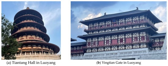
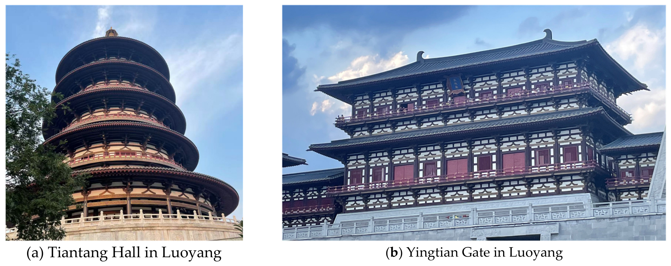
Traditional Chinese buildings are renowned for their timber-frame systems and distinctive architectural forms, in which components such as beams, columns, bracket sets, and brackets collectively form an architectural system with distinctive cultural characteristics. However, traditional timber structures suffer from several limitations, including insufficient durability, susceptibility to corrosion, and poor fire resistance [1]. In recent years, modern archaizing buildings have increasingly adopted advanced engineering materials, such as steel, to improve structural durability, construction efficiency, and safety performance while preserving the characteristic features of traditional architecture, as shown in Figure 1. Compared with traditional timber structures, steel structures exhibit higher strength, better ductility, and advantages in industrialized construction, making them a promising structural system for modern archaizing buildings.
Figure 1.
Modern archaizing buildings.
Unlike conventional steel frame structures, beam–column joints in steel archaizing buildings are influenced by traditional architectural forms and spatial configurations. These joints usually incorporate bracket sets, brackets, and beam members at different elevations, resulting in more complex load-transfer paths and local stress states within the joint regions [2]. At present, welded rigid connections are commonly adopted for such joints. Although these connections can satisfy the requirements for overall stiffness and load-bearing capacity, residual stresses and stress concentrations are likely to occur in welded regions. Under cyclic loading, local yielding, crack propagation, and even brittle failure may occur in the beam-end plastic regions and welded connection areas, thereby reducing the ductility and energy dissipation capacity of the joints.
Previous studies on steel archaizing building joints have mainly focused on the seismic performance of transition connections, overall frame structures, and beam–column joints. Xue et al. [3] conducted quasi-static tests on transition steel connections between rectangular and circular columns. The results demonstrated that these connections could satisfy the requirements for elastic–plastic deformation capacity specified in steel design codes. Subsequently, seismic tests were performed on steel archaizing building frame structures [4], revealing that structural damage was mainly concentrated in the beam-end flange and web regions, while the structures exhibited satisfactory load-bearing capacity and collapse resistance. In addition, investigations on double beam–column joints in steel archaizing buildings [5,6] indicated that the beam-end plastic hinge region was the primary damage zone. Under large deformation cyclic loading, flange tearing and fracture could occur in this region, resulting in degradation of joint ductility and energy dissipation capacity.
To mitigate earthquake-induced damage in steel joints, previous studies have proposed various structural modifications, such as reduced beam sections and flange reinforcement, to relocate plastic deformation regions and reduce the risk of failure near welded zones. These approaches can improve the seismic performance of conventional steel frame joints. However, for steel archaizing buildings, direct application of these methods may affect the architectural appearance and the arrangement of traditional components due to specific structural configurations and aesthetic requirements. Therefore, developing seismic enhancement strategies that consider both traditional architectural characteristics and structural performance is of great importance.
In recent years, supplemental energy dissipation devices have been explored to improve the seismic performance of steel joints in traditional-style buildings. Yuan et al. [7,8] proposed energy dissipation solutions based on SMA bar-friction dampers and rotary friction dampers for steel joints in archaizing buildings. Experimental results demonstrated that the incorporation of supplemental dampers could effectively improve hysteretic behavior, energy dissipation capacity, and residual deformation control. Qi et al. [9] investigated semi-rigid steel joints equipped with shear dampers in archaizing buildings and evaluated the influence of energy dissipation devices on seismic performance. These studies indicate that supplemental dampers provide an effective approach for enhancing the seismic performance of steel joints in archaizing buildings.
Among various energy dissipation devices, viscous dampers exhibit velocity-dependent energy dissipation characteristics, stable output force, and limited influence on the initial stiffness of structures, and have been widely applied in structural vibration control. However, previous studies have mainly focused on conventional steel frames, reinforced concrete structures, and seismic mitigation of entire buildings, while investigations on the application of viscous dampers to specific joints in steel archaizing buildings remain limited.
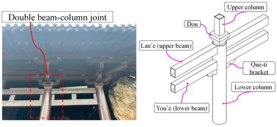
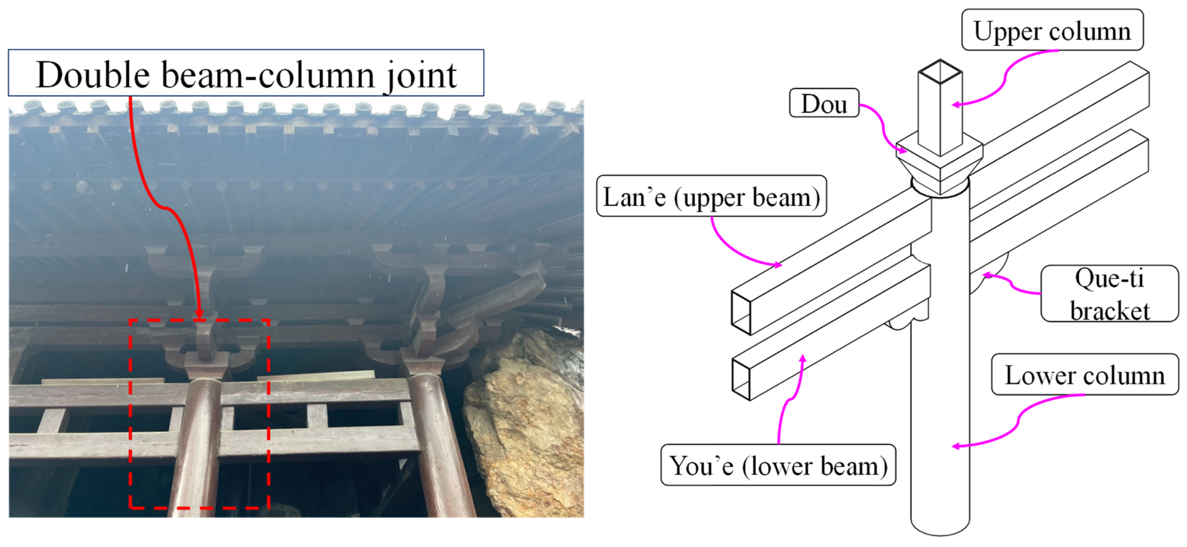
Que-ti brackets are located at the beam–column intersections of traditional buildings and possess unique spatial positions and structural configurations, as shown in Figure 2. Although Que-ti brackets in modern archaizing buildings mainly serve decorative functions, their locations provide potential installation spaces for supplemental energy dissipation devices. Installing viscous dampers in the bracket regions can provide additional energy dissipation capacity for beam–column joints without significantly altering the architectural appearance, thereby reducing damage in beam-end regions and welded connections [10].
Figure 2.
Structural configuration of the archaizing building joint.
For conventional structural components, various hysteretic models have been developed to describe cyclic responses, including skeleton curves, stiffness deterioration, and strength degradation behaviors [11,12,13,14,15,16,17]. Ibarra et al. [18] proposed a hysteretic model incorporating strength and stiffness deterioration, providing a theoretical basis for simulating cumulative damage behavior of structural components. Lignos et al. [19] further developed nonlinear models considering cyclic deterioration characteristics of steel components and applied them to seismic response analyses of steel frame structures. These models have been widely used in nonlinear seismic analyses of steel components and frame structures. Recently, restoring force models have also been developed for traditional-style building structures and concrete joints equipped with dampers [20]. However, existing models mainly focus on conventional steel components or concrete joints, and their applicability to steel archaizing building joints equipped with viscous dampers remains unclear.
Therefore, four steel archaizing building joints equipped with viscous dampers, including two single-beam joints and two double-beam joints, were investigated in this study. Dynamic cyclic loading tests were conducted to evaluate their hysteretic responses and nonlinear deformation characteristics. Based on the experimental results, a restoring force model incorporating a trilinear skeleton curve, stiffness deterioration relationships, and hysteretic criteria was established, and its capability in reproducing the experimental skeleton curves was evaluated. The findings provide a reference for nonlinear seismic response analysis and performance evaluation of steel archaizing building joints equipped with viscous dampers.
2. Experimental Program
2.1. Specimen Design
Four steel archaizing building joint specimens equipped with viscous dampers were investigated in this study, including two single-beam joints (SBJ series) and two double-beam joints (DBJ series). The specimens were designated as SBJ-V60, SBJ-V88, DBJ-V60, and DBJ-V88, where “SBJ” and “DBJ” denote single-beam and double-beam joints, respectively, and the numbers following “V” represent the damping coefficients of the viscous dampers.
The specimens were designed based on a prototype steel archaizing building of a second-grade palace-style structure located in Xi’an, China. According to the ts’ai-fen modular system specified in the Song Dynasty architectural treatise Yingzao Fashi [21], the dimensions of the specimens were converted using a geometric scale ratio of 1:2.6.
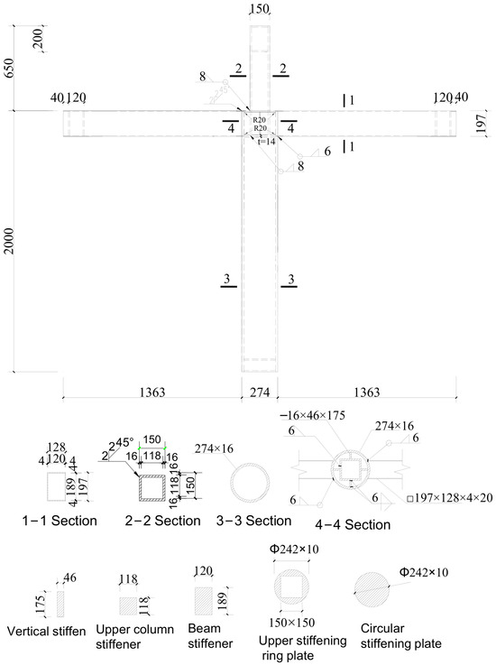
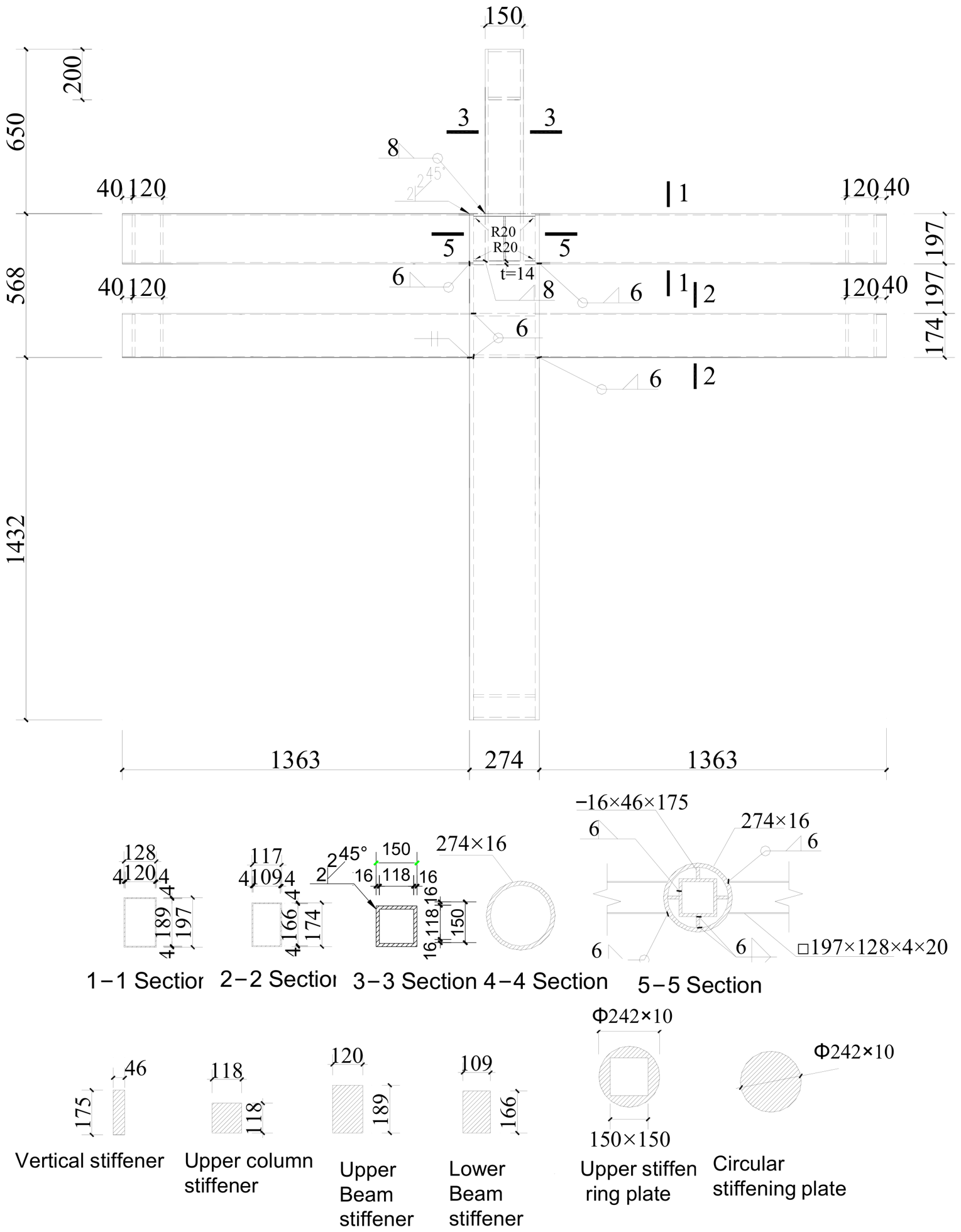
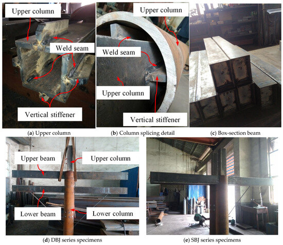
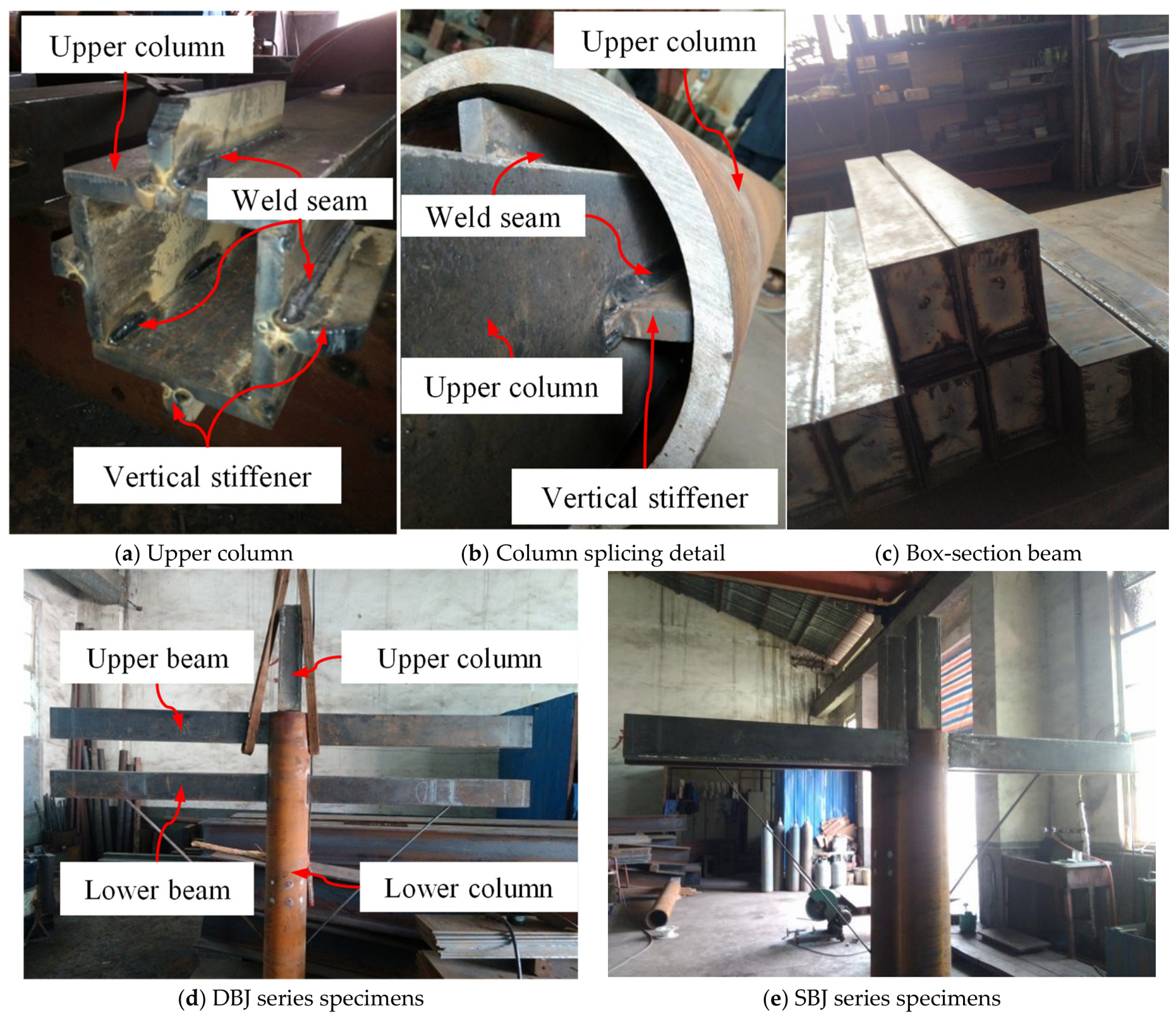
The detailed configurations and dimensions of the SBJ- and DBJ-series specimens are shown in Figure 3 and Figure 4, respectively. The main geometric parameters of the specimens are summarized in Table 1. The eave column consisted of a circular hollow section (CHS), while the lan’e (upper beam) and you’e (lower beam) were fabricated using welded box sections. A square hollow section (SHS) column was arranged above the joint and connected to the eave column through horizontal ring plates and vertical stiffeners, forming an integrated load-transfer system. This upper column was used for installing Dou-gong components and transferring loads from the upper structure. The total height and width of each specimen were 2650 mm and 3000 mm, respectively. The fabrication process of the specimens is shown in Figure 5.
Figure 3.
Detailed drawings of welds and dimensions of SBJ series specimens. Unit: mm.
Figure 4.
Detailed drawings of welds and dimensions of DBJ series specimens. Unit: mm.
Table 1.
Specimen details.
Figure 5.
On-site fabrication of joint specimens.
All beam–column connections were designed as fully welded rigid connections. The connection between the beams and CHS column was achieved using complete-joint-penetration groove welds. The CHS column and upper SHS column were connected through welded horizontal ring plates and vertical stiffeners. The fabrication and welding procedures complied with the requirements of the Code for Welding of Steel Structures (GB 50661) [22] and the Standard for Design of Steel Structures (GB 50017) [23].
2.2. Design of Viscous Dampers
The Que-ti bracket is generally located at the intersection between beams (lintels) and columns and typically has a triangular configuration. In traditional timber structures, it serves both decorative and auxiliary load-transfer functions. According to the dimensional rules of traditional architecture, the horizontal length of the Que-ti bracket is approximately one-quarter of the clear span width of the main bay, the vertical height is approximately half of its horizontal length, and the thickness is approximately three-tenths of the column diameter.
The specimens were designed based on a prototype second-grade palace-style steel archaizing building located in Xi’an, China. According to the ts’ai-fen modular system specified in the Song Dynasty architectural treatise Yingzao Fashi [21], the geometric dimensions of the specimens were converted using a scale ratio of 1:2.6. The main geometric parameters of the specimens were determined based on the traditional architectural scale system. The diameter of the eave column was 274 mm, and the width of the building bay was 3000 mm. According to the geometric relationship of the Que-ti bracket, the available horizontal installation space for the viscous damper was estimated to be approximately 0.7–0.9 m. Therefore, the damper length was specifically designed to satisfy this spatial limitation.
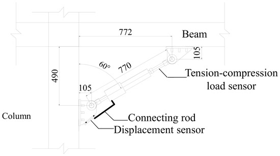
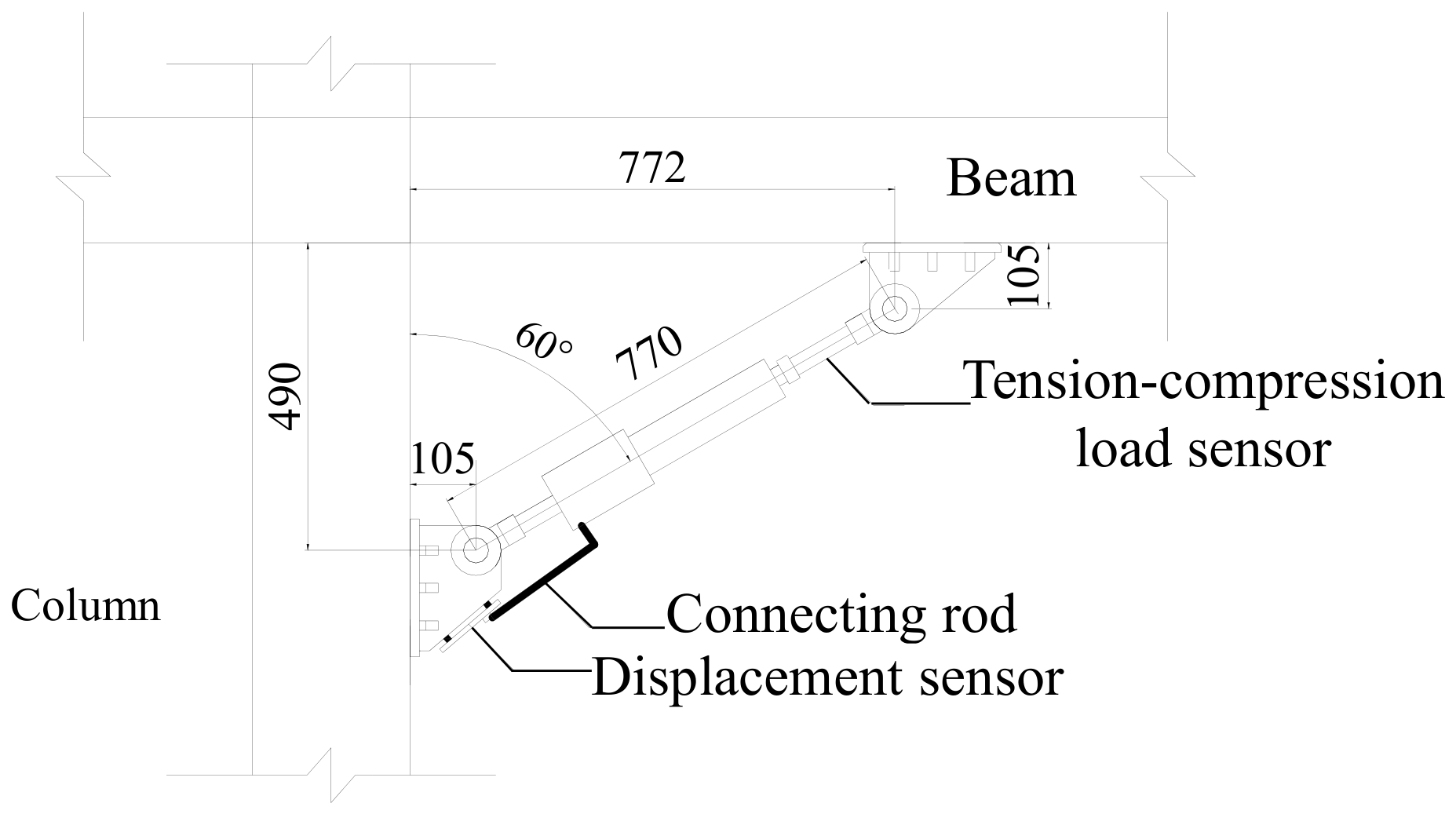
Considering that conventional engineering viscous dampers usually have relatively large dimensions and cannot be directly installed in scaled archaizing building joint specimens, the damper dimensions were determined through technical discussions with the manufacturer, considering both the experimental requirements and fabrication conditions. The effective length of the viscous damper was selected as 770 mm. After considering the dimensions of the connection brackets and the installation space required for displacement sensors, the overall horizontal span of the damper was 772 mm, which was generally consistent with the available space provided by the Que-ti bracket. The detailed configuration and dimensions of the viscous damper are shown in Figure 6.
Figure 6.
Detailed configuration of the viscous damper. Unit: mm.
To obtain the output force and relative displacement of the damper during loading, intelligent viscous dampers were adopted in the experiment. The damper consisted of a nonlinear viscous damping unit and a data acquisition system, and the internal sensors were capable of simultaneously recording the damping force and displacement response. The viscous damper was connected to the beam and column through double-clevis connection brackets, with an installation angle of 60°, as shown in Figure 2.
The mechanical behavior of the nonlinear viscous damper can be described by the following force–velocity relationship:
where F is the damping force, C is the damping coefficient, v is the relative velocity of the piston, and α is the velocity exponent.
F = CVα
In the present test program, the preliminary ranges of the damping coefficient and velocity exponent were first determined according to the selected damper dimensions, the performance parameters available from the manufacturer, and the expected dynamic response of the joint specimens. In the preliminary finite element analyses, the velocity exponent was initially taken as α = 0.30, while the damping coefficient C was initially set to 40 and then increased in increments of 5. The dynamic responses of the joint specimens under different damping parameters were calculated and compared. Based on the numerical trial results and the practical fabrication conditions of the dampers, two target damping coefficients, C = 60 and 88, were selected to investigate the influence of different damping levels. After fabrication, the dampers were subjected to performance testing by the manufacturer, and the measured velocity exponent was α = 0.38. Therefore, the final parameters adopted for the VD-60 and VD-88 dampers were C = 60 and 88 kN·(s/m), respectively, with α = 0.38, as summarized in Table 2.
Table 2.
Summary of design parameters of viscous dampers.
2.3. Material Testing
To obtain the mechanical properties of the steel used in the specimens, steel samples were extracted from the CHS columns, welded box beams, and SHS columns in accordance with the requirements of Hot-rolled Structural Steel Plate, Sheet and Strip—Sampling Location and Sample Preparation for Mechanical Testing (GB/T 2975-2018) [24]. Standard tensile coupons were then fabricated from the extracted samples.
The 4 mm thick steel plate coupons were used to determine the material properties of the welded box beam flanges and webs; the 16 mm thick steel plate coupons were used for the flanges and webs of the upper SHS columns; and the 16 mm thick steel tube coupons were used for the CHS columns.
The tensile tests were conducted according to Metallic Materials—Tensile Testing—Part 1: Method of Test at Room Temperature (GB/T 228.1-2021) [25]. The yield strength (fy), ultimate tensile strength (fu), elastic modulus (Es), and elongation (δ) of different steel materials were obtained. The dimensions of the tensile coupons and the test results are presented in Table 3.
Table 3.
Mechanical properties of steel materials.
2.4. Experimental Setup
A dynamic cyclic loading test was conducted using an MTS electro-hydraulic servo loading system to simulate the seismic response of steel archaizing building beam–column joints. During the test, a constant axial load was first applied at the top of the column through a vertical loading system, followed by cyclic dynamic loading at the beam end using a horizontal electro-hydraulic servo actuator. The vertical axial load was applied using a 1000 kN hydraulic jack. A roller device was installed between the hydraulic jack and the reaction beam to allow free horizontal movement of the column top during cyclic loading. The horizontal cyclic load was applied by a 500 kN electro-hydraulic servo actuator fixed to the reaction wall, with a maximum stroke of ±250 mm.
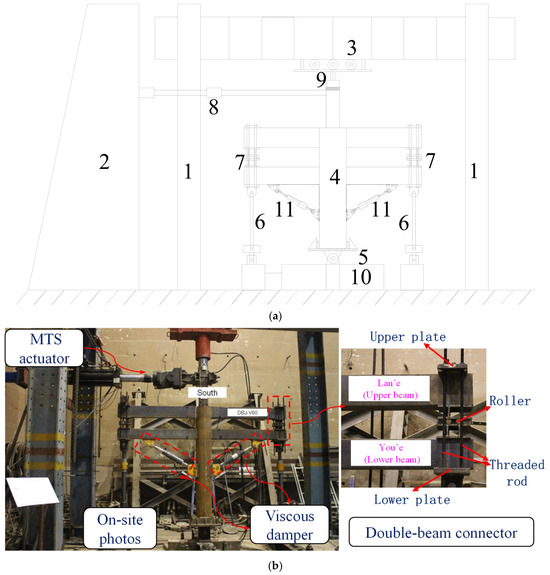
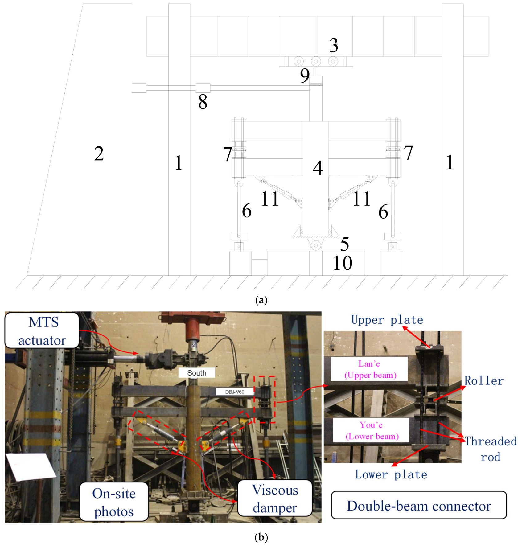
The test setup and loading process are shown in Figure 7. For the double-beam joint specimens, the beam-end locations correspond approximately to the inflection-point regions of the beams in the prototype structure. Therefore, the test boundary condition was designed to allow relative horizontal movement between the Lan’e and You’e beam ends while maintaining their prescribed vertical spacing. For this purpose, a specially designed double-beam connector was installed at the beam ends, as shown in Figure 7b. The upper and lower plates of the connector were connected to the Lan’e and You’e beams, respectively, through high-strength threaded rods, while rollers arranged between the two plates allowed free relative horizontal movement. Together with the vertical pin-ended tie rods shown as Component 6 in Figure 7a, this configuration enabled the Lan’e and You’e beam ends to move horizontally while maintaining the prescribed vertical spacing and minimizing additional shear and moment transfer between the two beams. Thus, the required beam-end boundary conditions and load-transfer characteristics of the prototype double-beam system could be reproduced during dynamic cyclic loading.
Figure 7.
Experimental setup: (a) Schematic diagram. 1. Reaction frame 2. Reaction wall 3. Reaction beam 4. Specimen 5. Hinged support 6. Tie rod 7. Double-beam connector 8. MTS electro-hydraulic servo actuator 9. Hydraulic jack 10. Foundation beam 11. Viscous damper; (b) Photograph of the experimental setup.
2.5. Loading Protocol
For the viscous damper-equipped joints investigated in this study, the damping force is strongly dependent on the loading velocity. Therefore, the dynamic response of the joints is governed not only by the deformation amplitude but also by the loading frequency. To accurately evaluate the influence of viscous dampers on the seismic performance of steel archaizing building joints, dynamic cyclic loading tests were conducted [26]. Considering the periodic characteristics and velocity-dependent effects of structural responses under earthquakes, as well as the control capability of the electro-hydraulic servo loading system, a sinusoidal dynamic loading scheme with displacement–frequency coupled control was adopted [27,28,29,30,31]. By varying the displacement amplitude and loading frequency, different deformation and velocity levels were achieved to investigate the nonlinear response characteristics of viscous damper-equipped joints under cyclic dynamic loading.
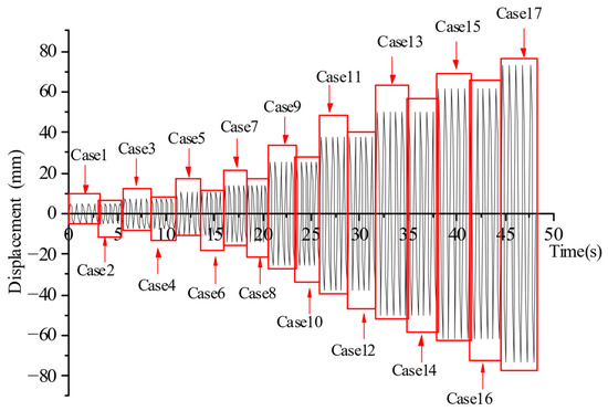
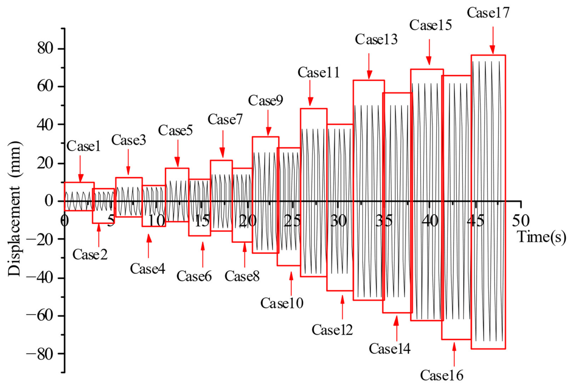
The loading protocol was designed based on previous studies [32,33] and the horizontal ground-motion parameters corresponding to different seismic intensity levels specified in the Seismic Intensity Scale of China (GB/T 17742-2020) [34]. Considering the specimen height of 2650 mm, the deformation characteristics of steel archaizing building joints, and the additional energy dissipation provided by viscous dampers, the displacement amplitudes were selected as 5, 8, 11, 15, 27, 40, 53, 65, 77, and 88 mm, representing different loading levels. The frequency parameters for each loading condition were determined according to the target displacement amplitudes and corresponding peak acceleration requirements. The detailed loading conditions are presented in Table 4 and Figure 8. During the test, continuous sinusoidal cyclic loading was applied at each displacement level, and five loading cycles were performed for each amplitude.
Table 4.
Loading scheme.
Figure 8.
Loading protocol.
2.6. Measurement Scheme
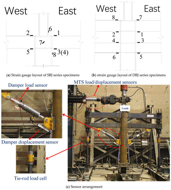
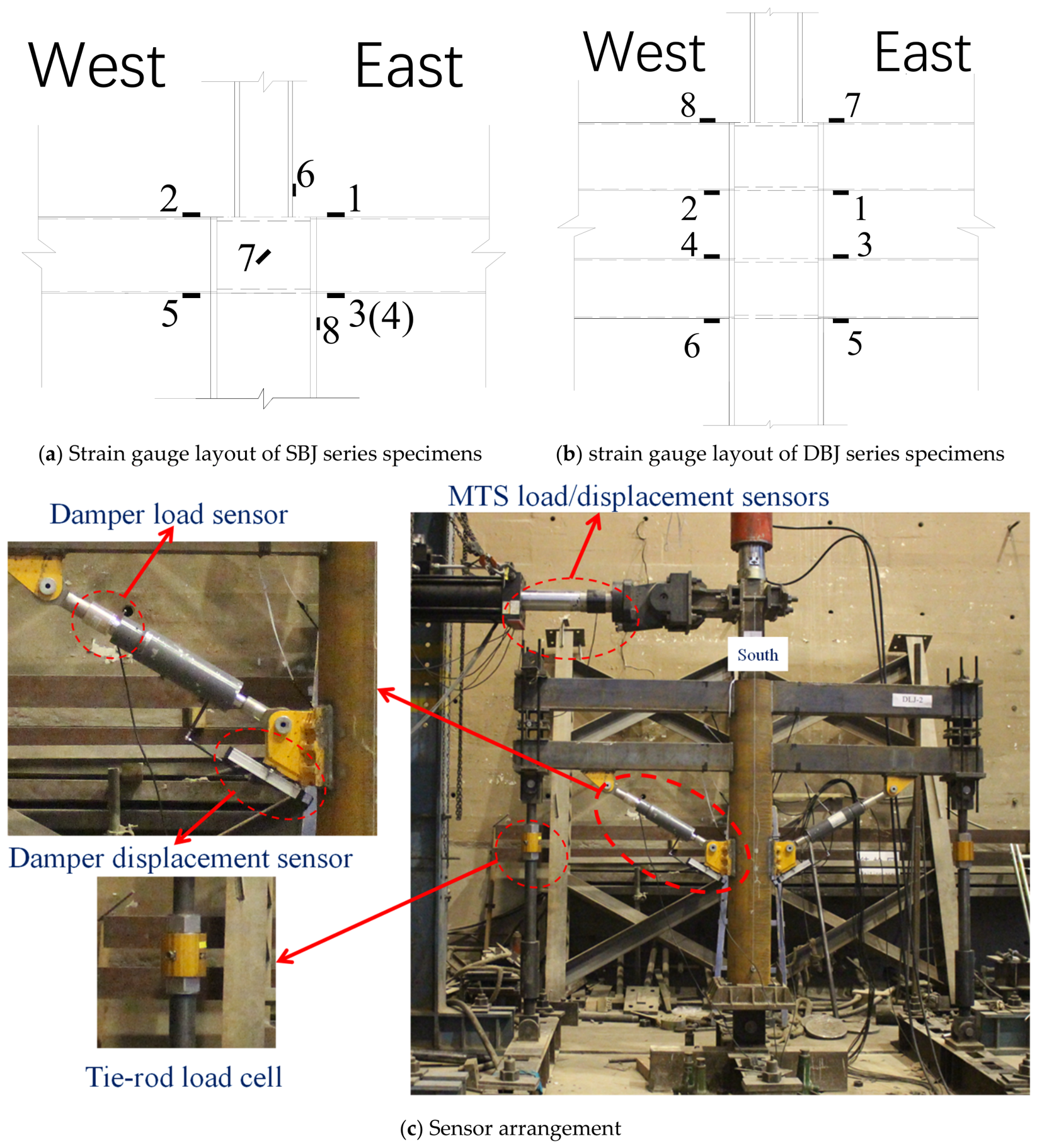
The specimens were designed and fabricated according to the strong-column weak-beam principle, and the beam-end plastic hinge regions were the primary focus of this study. Therefore, strain gauges were mainly installed in these regions to monitor the yielding behavior and plastic deformation development of the beam ends. For the SBJ series specimens, strain gauges were arranged at the upper and lower beam flanges, the base region of the upper square column, the joint core region, and the CHS column wall. The strain gauges on the beam flanges were located approximately 50 mm away from the beam end. Since dynamic cyclic loading was adopted in this study, the available dynamic strain acquisition system provided only eight channels for simultaneous measurement. For the SBJ series, only one beam level was present, so fewer strain gauges were required in the beam-end plastic hinge region. Therefore, additional gauges were placed at the base of the upper column and in the joint connection region to monitor whether yielding occurred outside the beam ends and to assess the intended strong-column–weak-beam behavior. The SBJ test results showed that Gauges 6 and 7 in these regions did not reach the yield strain. Based on this observation, the strain-gauge arrangement was adjusted for the subsequent DBJ tests. Since both the upper and lower beams participate in the response of the DBJ specimens, all eight available strain gauges were concentrated on the upper and lower beam flanges near the beam-end plastic hinge regions, which were the primary regions of interest for monitoring yielding and plastic deformation.
Since dynamic cyclic loading was adopted in this study, the load and displacement responses at the loading end were mainly measured using the integrated load and displacement sensors of the MTS actuator. In addition, a tension–compression load cell was installed on the tie rod at the beam end to monitor the axial force transmitted through the loading system. The intelligent viscous dampers were equipped with an integrated damper load sensor and a corresponding displacement sensor, which simultaneously recorded the damping force and relative displacement during the test. The detailed instrumentation layout is shown in Figure 9.
Figure 9.
Measurement arrangement of the specimens.
3. Test Results
3.1. Failure Modes
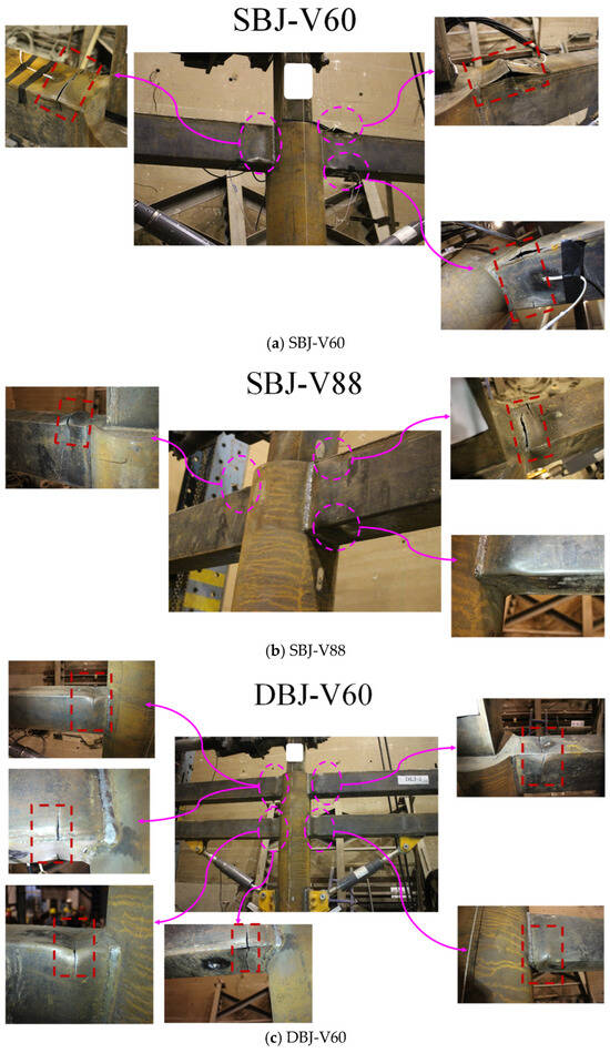
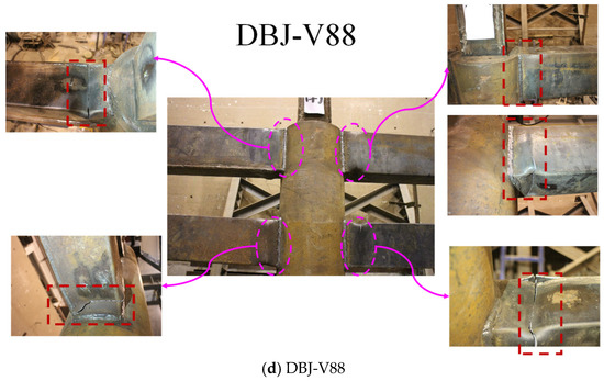
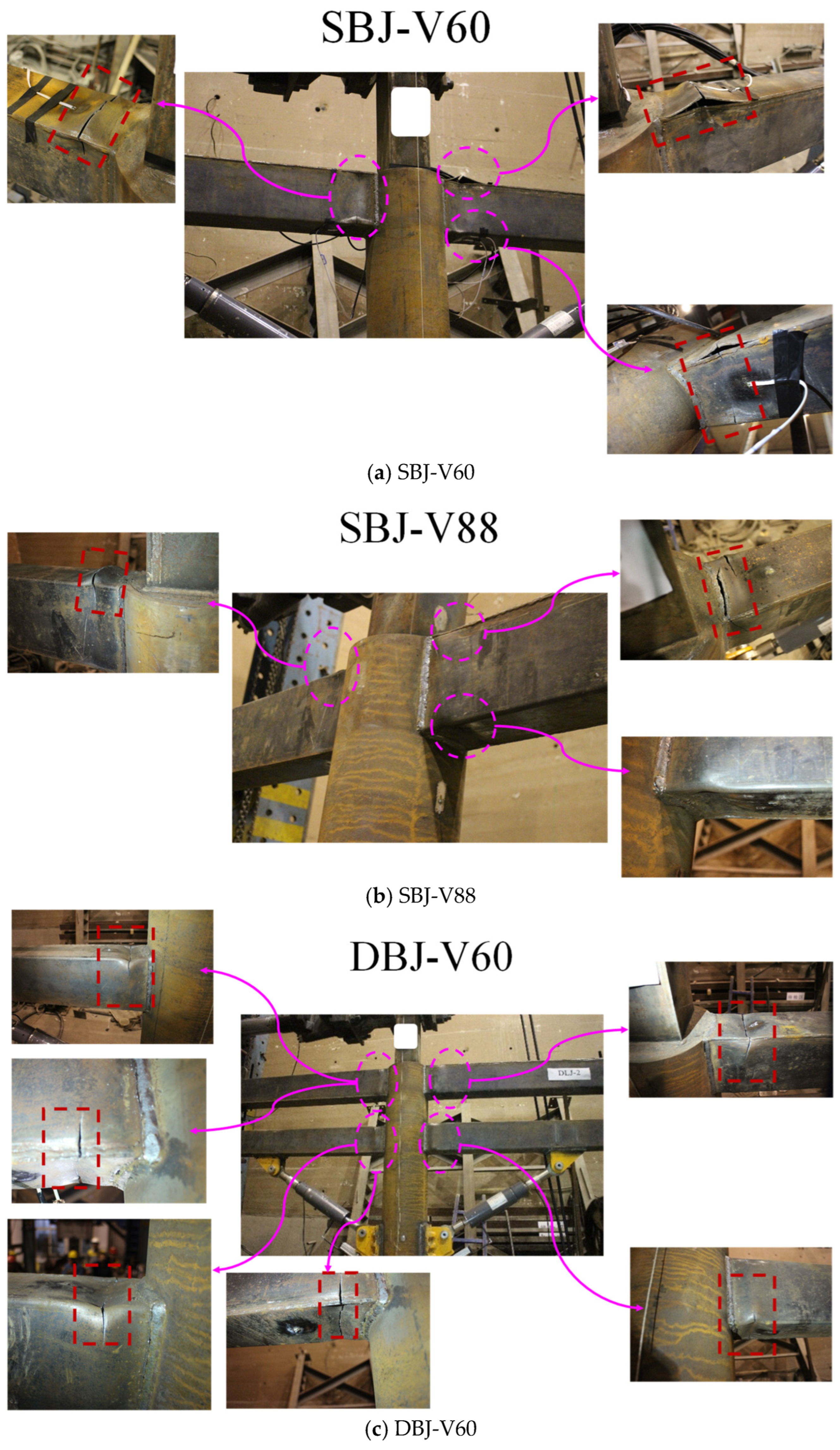
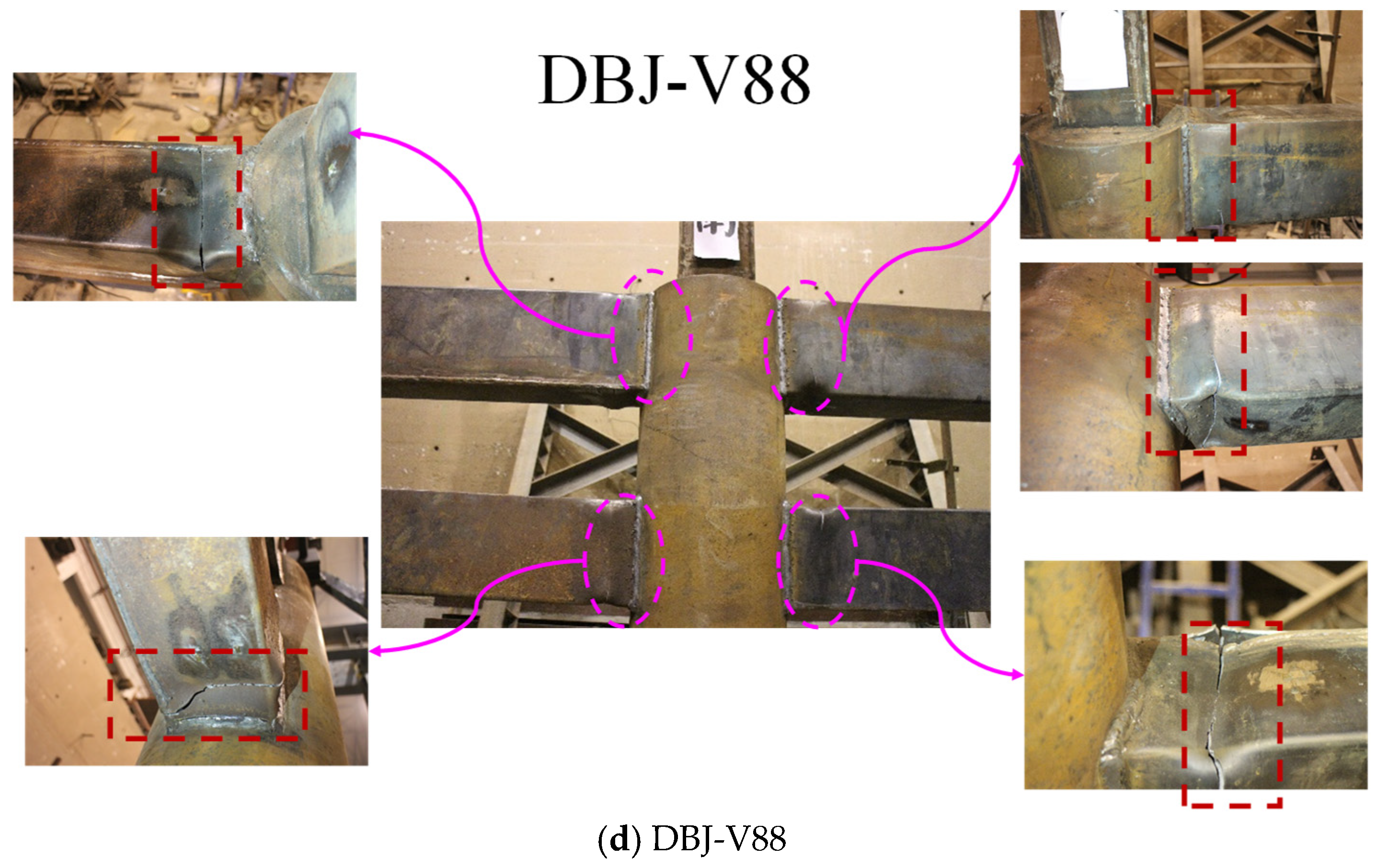
The failure modes of the four viscous damper-equipped joint specimens are shown in Figure 10. At the initial loading stage, the beam ends, columns, and joint regions of all specimens remained in the elastic state, and the relationship between the column-end load and displacement was approximately linear. When the imposed displacement increased to 27 mm, the beam-end plastic hinge regions gradually reached the yielding state, accompanied by an obvious change in the load–displacement response, indicating the transition from elastic to elastoplastic behavior. With further increase in displacement amplitude, plastic deformation gradually concentrated in the beam-end regions. Local buckling and out-of-plane deformation first occurred in the beam flanges and webs, followed by crack initiation in the damaged regions. The cracks propagated progressively under cyclic loading, resulting in a gradual degradation of the load-carrying capacity.
Figure 10.
Failure modes of specimens.
For the single-beam–column joints SBJ-V60 and SBJ-V88, the primary damage was concentrated in the beam-end plastic hinge regions approximately 30–90 mm away from the beam–column welded connection. For SBJ-V60, initial cracks were observed at the flange-web connection region when the displacement amplitude reached 53 mm. Subsequently, the cracks gradually propagated into the beam flange and web during subsequent loading cycles. For SBJ-V88, the beam-end regions mainly exhibited local buckling of the flange and web at displacement amplitudes of 40–53 mm. When the displacement amplitude increased to 65 mm, tearing of the steel material initiated in the buckled regions and further developed into through-thickness cracks at the 77 mm loading stage. No significant damage was observed in the welded beam–column connection regions for either specimen, and the final damage was mainly concentrated within the beam-end plastic hinge regions.
For the double-beam–column joints DBJ-V60 and DBJ-V88, damage occurred simultaneously in the upper and lower beam ends due to the interaction between the two beams. After yielding, local buckling gradually developed in the beam flanges and webs, accompanied by the initiation and propagation of cracks in the steel material. DBJ-V60 exhibited apparent local buckling at a displacement amplitude of 53 mm, followed by progressive crack propagation under larger displacement cycles, leading to severe damage during the 77–88 mm loading stages. For DBJ-V88, local buckling and initial cracking occurred at displacement amplitudes of 40–53 mm. With increasing displacement, the cracks further propagated toward the web regions and eventually resulted in partial fracture of the beam flanges. Compared with the single-beam–column joints, the damage of the double-beam–column joints was more widely distributed due to the contribution of both upper and lower beams; however, the critical damage remained concentrated in the beam-end plastic hinge regions.
The specimens were designed according to the strong-column–weak-beam principle, and the beam–column connection regions were strengthened by horizontal ring plates and vertical stiffeners. Therefore, during cyclic loading, the columns and joint core regions retained sufficient stiffness and strength, while plastic deformation gradually concentrated in the adjacent beam-end regions. After yielding, the beam flanges and webs were repeatedly subjected to tension and compression. Local buckling first occurred in the compressed regions and became more pronounced with increasing displacement amplitude. With continued cyclic loading, plastic deformation accumulated in the buckled regions, leading to crack initiation and subsequent propagation in the beam-end base metal. No evident cracking was observed in the beam–column complete-joint-penetration welds of the present specimens. The viscous dampers provided additional velocity-dependent resistance and contributed to energy dissipation during cyclic loading. At large deformation levels, however, progressive local buckling and base-metal cracking at the beam ends eventually led to strength degradation and governed the final failure of the joints.
Overall, the four specimens exhibited a consistent beam-controlled failure mechanism, with damage concentrated in the beam-end plastic hinge regions while the columns, joint core regions, and beam–column welds remained essentially intact. The observed damage evolution provides the physical basis for defining the characteristic points and degradation behavior adopted in the subsequent restoring force model.
3.2. Hysteretic Behavior
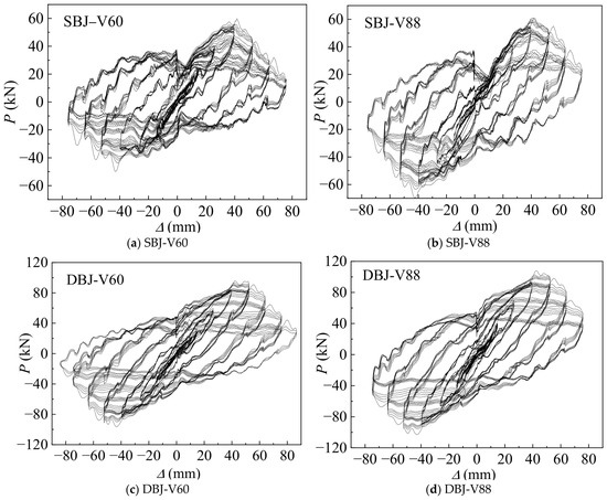
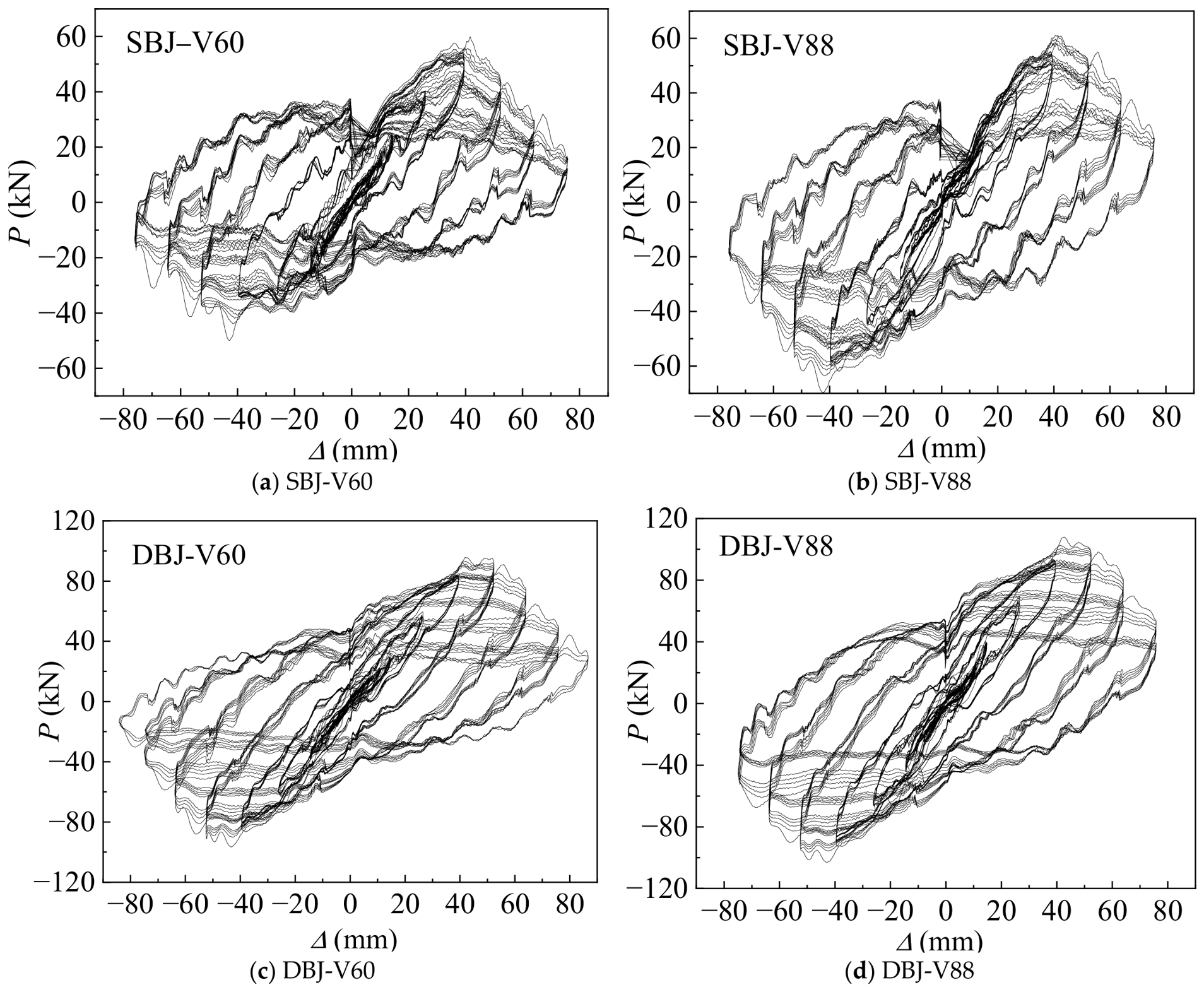
Figure 11 presents the column-end load–displacement hysteretic curves of the four viscous damper-equipped joint specimens. Overall, all specimens exhibited stable and continuous hysteresis loops with an approximately spindle-shaped configuration. No obvious pinching effect was observed, indicating favorable cyclic deformation capacity and energy dissipation performance. Since sinusoidal displacement-controlled dynamic loading was adopted in this study, slight fluctuations appeared at the edges of the hysteretic curves. This phenomenon was mainly associated with the closed-loop control of the electro-hydraulic servo loading system and the variation in loading velocity, but it did not affect the overall shape or primary mechanical characteristics of the hysteretic curves.
Figure 11.
Hysteretic curve of specimens.
At the initial loading stage, the relationship between the column-end load and displacement was approximately linear, and the hysteresis loops enclosed relatively small areas, indicating that the joints remained in the elastic stage. When the controlled displacement increased to approximately 27 mm, yielding initiated in the beam-end plastic hinge regions, accompanied by an evident change in the hysteretic curves. Residual deformation occurred after unloading, indicating that the joints entered the elastic–plastic stage. With further increases in displacement amplitude, the beam-end plastic regions gradually expanded, and local buckling and base metal cracking developed in the beam flanges and webs. Meanwhile, the hysteresis loop areas continuously increased, while the unloading stiffness gradually decreased, demonstrating apparent stiffness degradation.
At each displacement amplitude, five loading cycles were applied. With increasing cycle number, the peak loads and slopes of the hysteresis loops gradually decreased, and the hysteresis curves within the same loading level no longer completely overlapped. This indicated that cumulative damage developed in the joints under cyclic dynamic loading, accompanied by strength and stiffness degradation. Nevertheless, all specimens maintained stable hysteretic responses throughout the loading process, without obvious pinching behavior or sudden instability.
Overall, the four specimens exhibited similar hysteretic evolution characteristics, including three typical stages: the elastic stage, yielding stage, and degradation stage. The hysteretic curves effectively reflected the nonlinear characteristics associated with beam-end plastic development, stiffness degradation, and strength degradation, providing experimental evidence for the subsequent establishment of the skeleton curves, stiffness degradation relationships, and hysteretic rules of the restoring force model.
3.3. Skeleton Curve
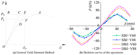
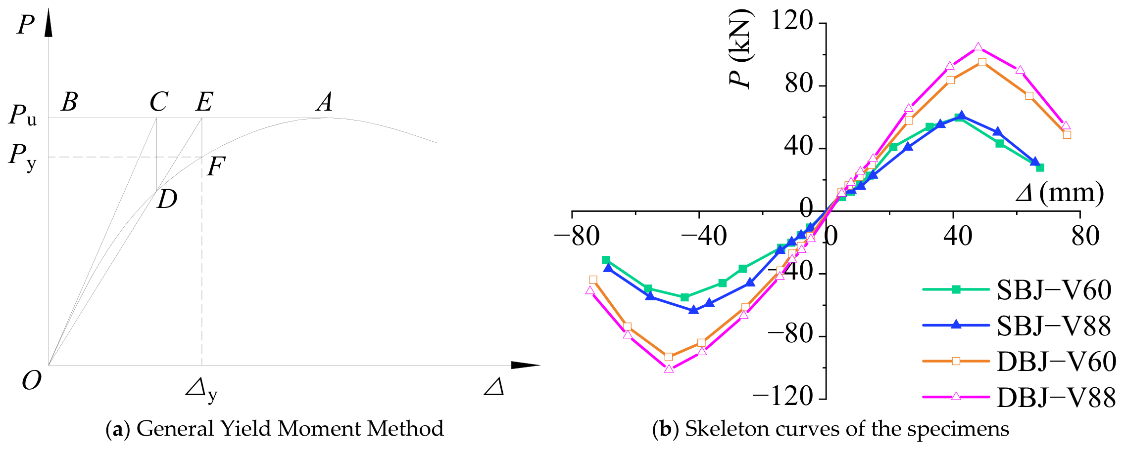
To establish the restoring force model, the key characteristic parameters of the skeleton curves, including the yield point, ultimate point, and failure point, should be determined. The yield point represents the transition from elastic response to nonlinear behavior, while the ultimate point corresponds to the peak load capacity of the joint. According to the Specification for Seismic Test of Buildings (JGJ/T 101-2015) [26], the failure point was defined as the point corresponding to a reduction in the load to 85% of the peak load. In this study, the General Yield Moment Method was adopted to determine the yield points of the specimens, as illustrated in Figure 12a. First, a horizontal line AB was drawn through the peak-load point A of the P–Δ skeleton curve, and the corresponding load was defined as the ultimate load Pu. A tangent line OC was then drawn from the origin O to the initial ascending branch of the skeleton curve and intersected AB at Point C. A vertical line through Point C intersected the skeleton curve at Point D. Line OD was subsequently extended to intersect AB at Point E. Finally, a vertical line through Point E intersected the skeleton curve at Point F. The ordinate and abscissa of Point F were taken as the yield load Py and yield displacement Δy, respectively. The obtained characteristic parameters are summarized in Table 5, and the skeleton curves of all specimens are shown in Figure 12b.
Figure 12.
Determination of characteristic points and skeleton curves of the specimens.
Table 5.
Characteristic points of all specimens.
It can be observed that the four viscous damper-equipped joint specimens exhibited similar overall skeleton characteristics, with three typical stages including the elastic stage, strengthening stage, and degradation stage. During the elastic stage, the relationship between the column-end load and displacement remained approximately linear, and all specimens exhibited relatively high initial stiffness. After reaching the yielding state, the skeleton curves gradually deviated from linear behavior, accompanied by a continuous reduction in curve slope. This indicates that the beam-end plastic hinges initiated and progressively developed, and the joints entered the elastoplastic development stage. With further increases in displacement, local buckling and crack propagation in the beam flanges and webs became increasingly significant after the peak load was reached. Consequently, the load-carrying capacity gradually decreased, and the skeleton curves entered the degradation stage.
As summarized in Table 5, the four specimens exhibited similar characteristic displacement ranges. The yield displacements were mainly distributed between 28 and 33 mm, while the ultimate displacements and failure displacements were approximately 43–50 mm and 53–62 mm, respectively. This indicates that the specimens experienced similar nonlinear development processes despite differences in joint configurations and damper parameters. Compared with the single-beam–column joints (SBJ series), the double-beam–column joints (DBJ series) exhibited higher yield loads, ultimate loads, and failure loads, indicating that the interaction between the upper and lower beams enhanced the overall load-carrying capacity. For specimens with the same joint configuration, the specimens equipped with larger damper coefficients (SBJ-V88 and DBJ-V88) exhibited slightly higher peak loads than the corresponding specimens with smaller damper coefficients (SBJ-V60 and DBJ-V60), indicating that damper parameters influenced the additional energy dissipation capacity and peak response during cyclic loading.
Overall, the four viscous damper-equipped joint specimens exhibited stable and consistent three-stage skeleton characteristics. These results indicate that the nonlinear response of this type of joint can be reasonably represented using a three-segment backbone curve. Therefore, the subsequent restoring force model adopts the three-segment backbone curve as the basic form and further incorporates stiffness degradation relationships and hysteretic rules.
4. Development of Restoring Force Model
4.1. Backbone Curve Model
Based on the dynamic loading test results of viscous damper-equipped joints, a restoring force model was developed to describe the overall nonlinear load–deformation relationship of this type of joint, providing a basis for nonlinear seismic response analysis of steel archaizing buildings.
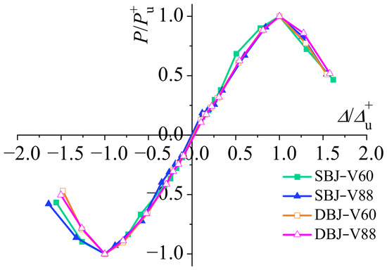
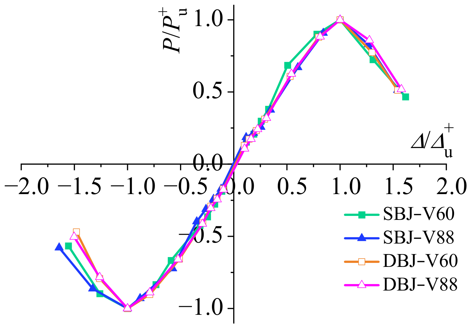
To establish a unified restoring force model, the skeleton curves of the four viscous damper-equipped joint specimens were first normalized. The normalized load P/Pu was adopted as the vertical axis, and the normalized displacement Δ/Δu was used as the horizontal axis. Here, Pu and Δu represent the ultimate load and the corresponding displacement obtained from the tests, respectively, and the ultimate points were determined according to the method described in Section 3.3. P and Δ represent the load and displacement responses during cyclic loading.
The normalized skeleton curves of all specimens are shown in Figure 13. It can be observed that although the specimens exhibited different absolute load capacities and deformation capacities, the normalized skeleton curves showed good consistency. All specimens exhibited three typical stages, including elastic development, post-yield strengthening, and post-peak degradation. Therefore, a unified three-segment backbone curve can reasonably describe the nonlinear response of steel archaizing building joints equipped with viscous dampers.
Figure 13.
Normalized skeleton curves of the tested joints.
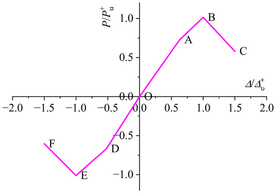
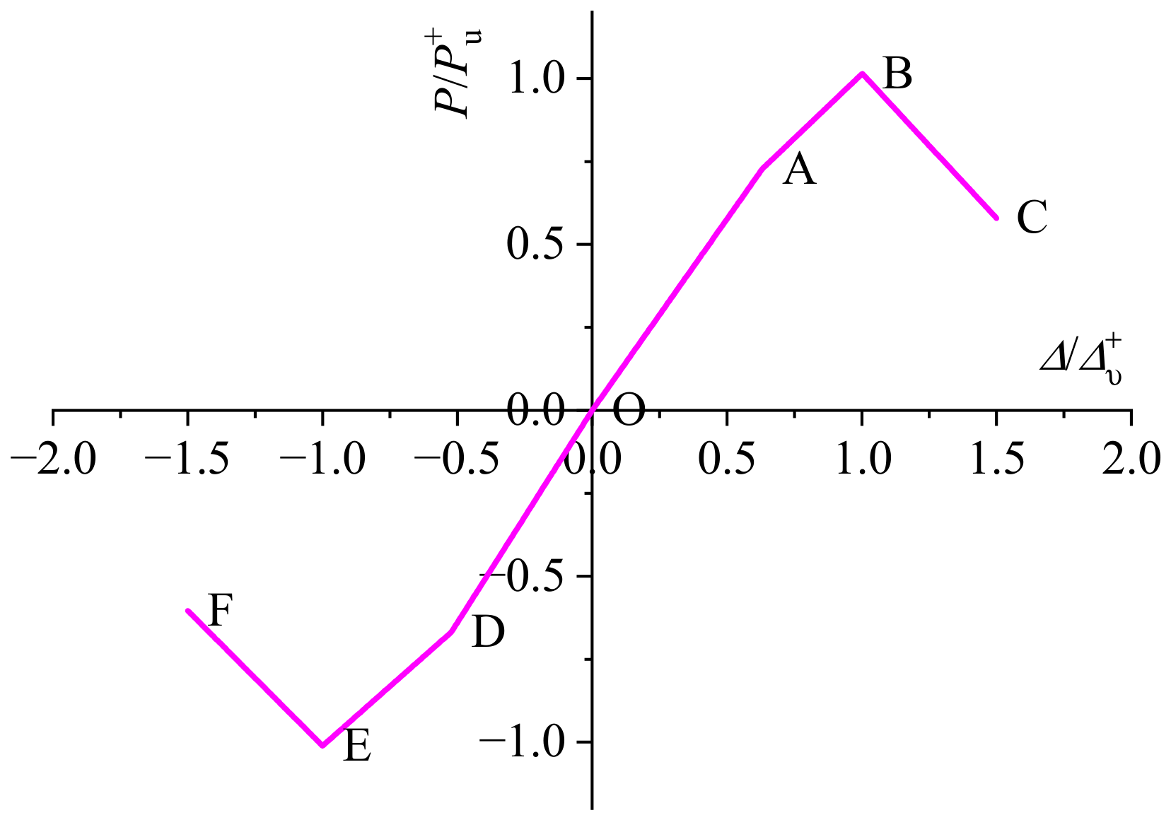
It should be noted that the three stages of the proposed backbone curve represent not only the overall load–deformation relationship but also the evolution of different mechanical mechanisms in viscous damper-equipped joints. The first stage (OA segment) corresponds to the elastic response stage, during which no significant plastic deformation occurs in the beam–column connection region. The viscous damper begins to dissipate energy, while the main steel structure maintains relatively high stiffness. The second stage (AB segment) represents the post-yield strengthening stage. With the gradual formation of beam-end plastic hinges, the steel components enter the nonlinear response stage, while the viscous dampers continuously provide additional energy dissipation, allowing the joint to maintain increasing load-carrying capacity. The third stage (BC segment) corresponds to the post-peak degradation stage, during which local buckling and base metal damage in the beam-end regions progressively develop. Although the viscous dampers continue to dissipate energy, they cannot fully compensate for the degradation in load capacity caused by accumulated structural damage.
Figure 14 illustrates the three-segment backbone curve model adopted for the viscous damper-equipped steel archaizing building joints investigated in this study. To determine the parameters of each segment, linear regression was performed based on the experimental skeleton curve data. Due to fabrication tolerances, initial loading conditions, and measurement uncertainties, the experimentally obtained skeleton curves did not always pass through the origin. Therefore, the theoretical origin point (0,0) was introduced as a constraint condition during the fitting process to improve the consistency between the backbone curve model and the actual mechanical response.
Figure 14.
Trilinear skeleton curve model.
Taking the positive elastic segment OA as an example, linear regression was conducted using the experimental data of the four viscous damper-equipped joint specimens, and the fitted equation of the OA segment was obtained as follows:
The coefficient of determination R was 0.9855, indicating a high correlation between the fitted curve and the experimental results. Subsequently, the slope of the fitted line was modified to ensure that the line passed through the origin, resulting in the corrected equation of the OA segment:
Using the same procedure, the linear equations and parameters of the remaining segments of the three-segment backbone curve were obtained, and the results are summarized in Table 6. Compared with the positive branch, the normalized negative post-peak curves showed greater scatter, particularly in the EF segment. Nevertheless, the four specimens exhibited the same overall degradation trend, and no clear separation between the SBJ and DBJ series was observed; therefore, a unified regression equation was adopted to represent the average negative post-peak response.
Table 6.
Linear equations of the skeleton curve model.
As shown in Table 6, the parameters of the positive and negative backbone curves exhibited certain differences, indicating asymmetric responses of the viscous damper-equipped steel archaizing building joints under positive and negative loading directions. This difference may be attributed to variations in joint configuration, fabrication tolerances, and initial conditions during dynamic cyclic loading. Therefore, independent fitting parameters for the positive and negative directions were adopted to improve the accuracy of the proposed restoring force model in representing the actual joint response.
4.2. Stiffness Degradation Model
After entering the plastic stage, local buckling at the beam ends, crack propagation in the base metal, and cumulative damage under cyclic loading lead to progressive degradation of the unloading and reloading stiffness of the joints. To describe the stiffness degradation behavior of the viscous damper-equipped steel archaizing building joints, four characteristic stiffness parameters were defined according to Figure 15, including the positive unloading stiffness K1, negative reloading stiffness K2, negative unloading stiffness K3, and positive reloading stiffness K4. Each stiffness parameter was determined based on the slope of the corresponding loading or unloading path between two characteristic points.
Figure 15.
Definition of loading and unloading stiffness parameters.
To quantitatively characterize the stiffness degradation relationships, normalized parameters were adopted. The horizontal axis was defined as the ratios of unloading displacements Δ1, Δ3 and reloading displacements Δ2, Δ4 to the corresponding ultimate displacements, while the vertical axis was defined as the ratios of the degraded stiffness values K1, K2, K3, and K4 to the initial stiffness K0. The initial positive and negative stiffness values K0+ and K0− of each specimen were obtained through linear regression of the elastic-stage experimental data during dynamic loading, corresponding to the positive OA segment and negative OD segment in Figure 15, respectively. Based on the normalized experimental results, the stiffness exhibited an evident nonlinear degradation trend with increasing deformation. Therefore, nonlinear regression was performed to establish continuous degradation relationships for the unloading and reloading stiffness, following the regression-based approach reported in previous studies [35].
(1) Degradation relationship of K1
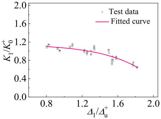
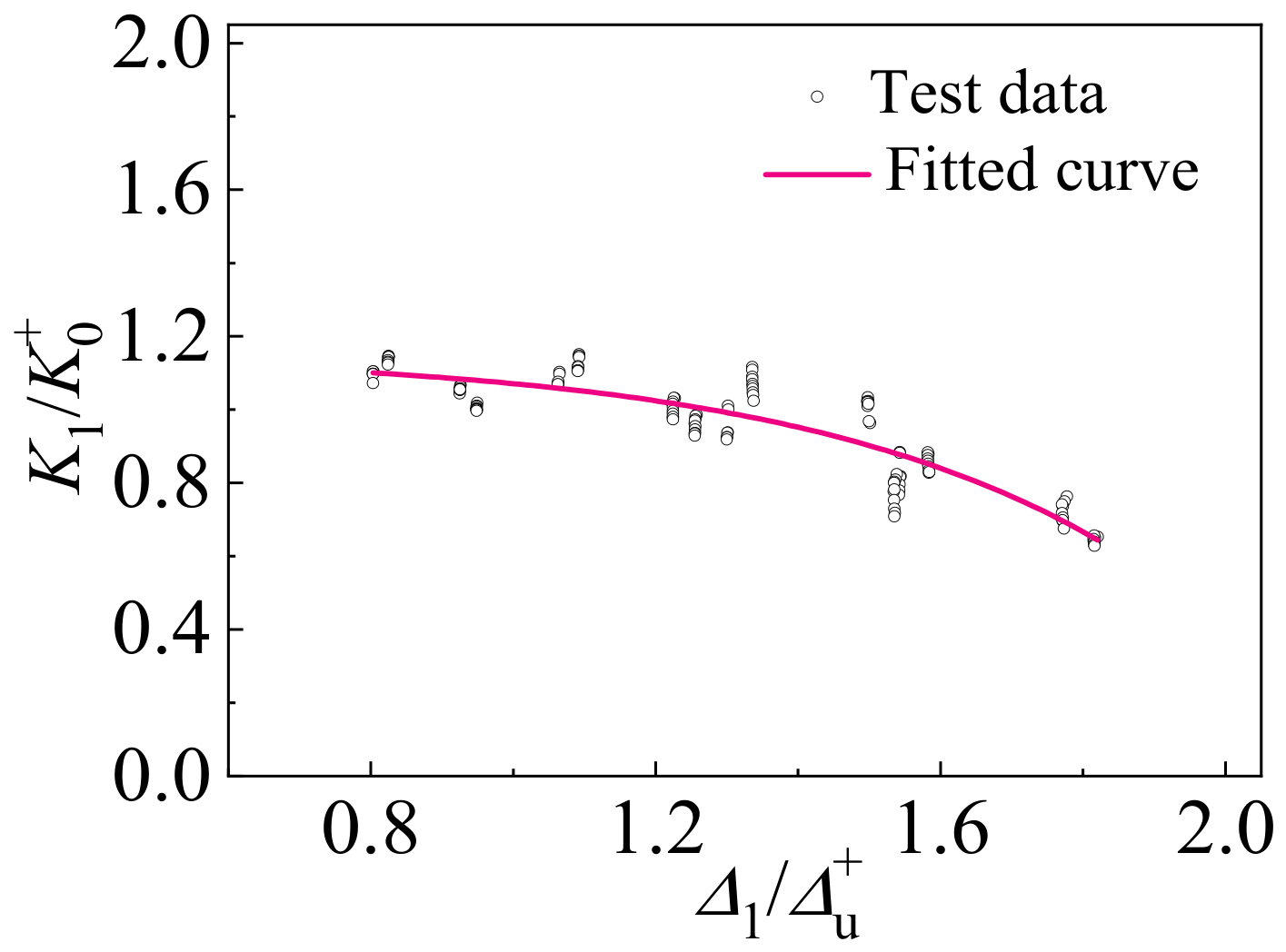
The degradation relationship of the positive unloading stiffness K1 was described by the relationship between K1/K0+ and Δ1/Δu+. The unloading stiffness K1 was first determined from the slope between the positive maximum displacement point (Point 1) and the point where the load decreased to zero (Point 2). Subsequently, the stiffness and displacement parameters were normalized, and an exponential function was adopted to fit the degradation relationship. The degradation curve of K1 is shown in Figure 16.
Figure 16.
Degradation relationship of positive unloading stiffness.
The degradation equation of K1 can be expressed as:
(2) Degradation relationship of K2
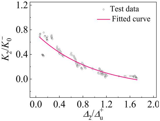
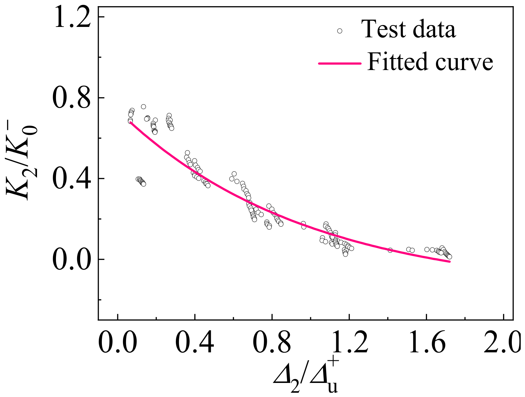
The degradation relationship of the negative reloading stiffness K2 was described by the relationship between K2/K0− and Δ2/Δu+. The reloading stiffness K2 was determined from the slope between the zero-load point (Point 2) and the negative loading characteristic point (Point 3). The normalized data were then fitted using an exponential function, and the degradation curve of K2 was obtained, as shown in Figure 17.
Figure 17.
Degradation relationship of negative reloading stiffness.
The degradation equation of K2 can be expressed as:
(3) Degradation relationship of K3
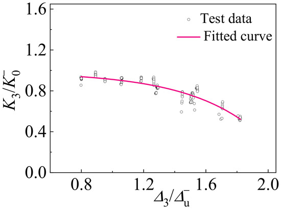
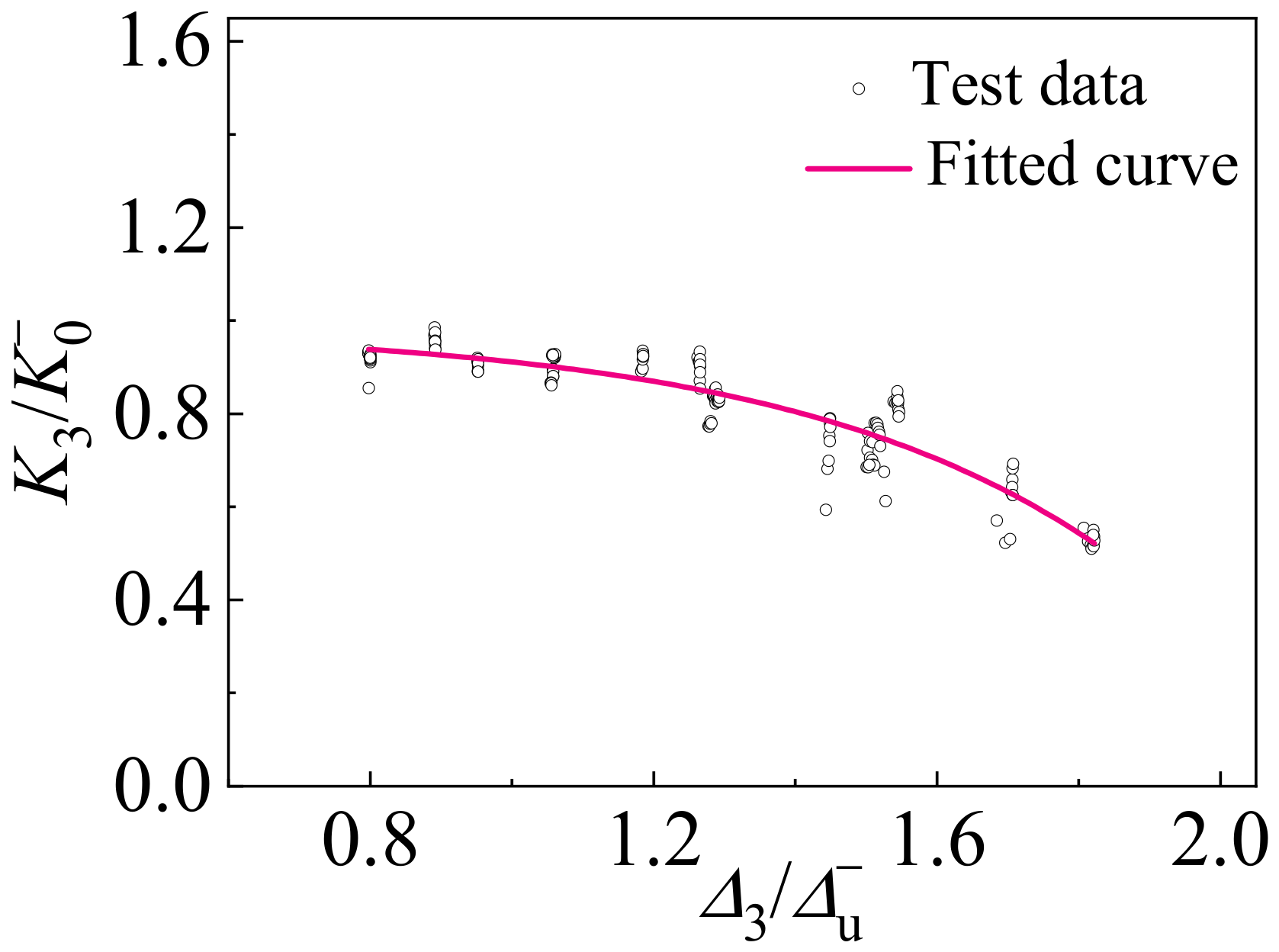
The degradation relationship of the negative unloading stiffness K3 was described by the relationship between K3/K0− and Δ3/Δu−. The unloading stiffness K3 was calculated from the slope between the negative maximum displacement point (Point 3) and the zero-load point (Point 4). After normalization of the stiffness and displacement parameters, the degradation relationship of K3 was obtained using exponential regression, as shown in Figure 18.
Figure 18.
Degradation relationship of negative unloading stiffness.
The degradation equation of K3 can be expressed as:
(4) Degradation relationship of K4
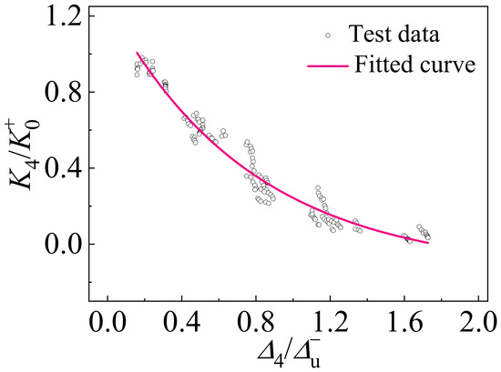
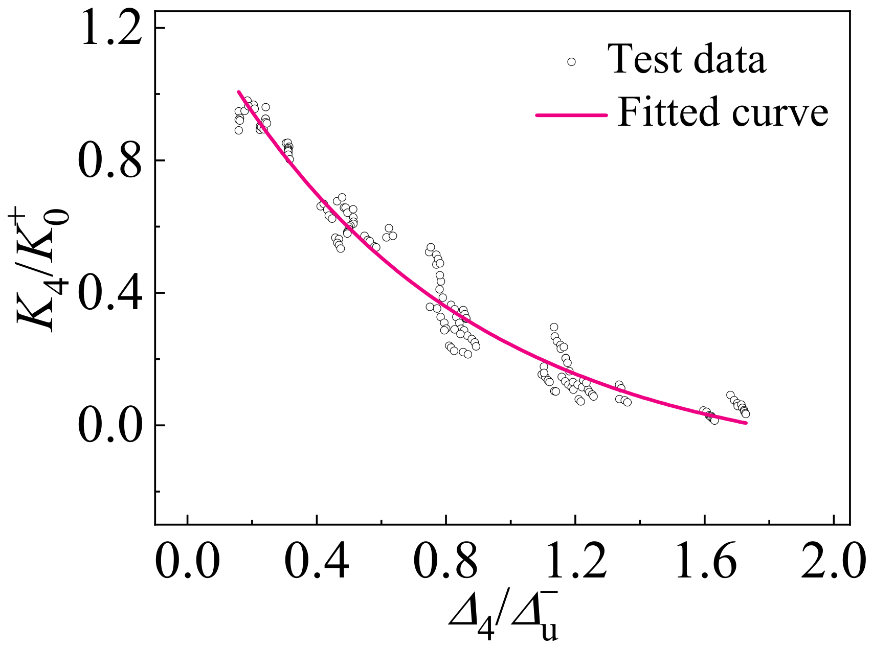
The degradation relationship of the positive reloading stiffness K4 was described by the relationship between K4/K0+ and Δ4/Δu−. The reloading stiffness K4 was determined from the slope between the zero-load point (Point 4) and the positive maximum displacement point (Point 1). The normalized data were fitted using an exponential function to obtain the degradation curve of K4, as shown in Figure 19.
Figure 19.
Degradation relationship of positive reloading stiffness.
The degradation equation of K4 can be expressed as:
4.3. Hysteretic Rules of the Restoring Force Model
Since the viscous dampers and steel joints investigated in this study form an integrated load-carrying system through the connecting supports, the experimentally obtained load–displacement responses incorporate the combined effects of steel joint deformation and energy dissipation provided by the viscous dampers. Therefore, a macroscopic restoring force model was developed in this study, in which the backbone curve was used to describe the evolution of load-carrying capacity, while the stiffness degradation relationships were adopted to characterize the cumulative damage effects under cyclic loading. The proposed model aims to simulate the nonlinear dynamic response of viscous damper-equipped steel archaizing building joints.
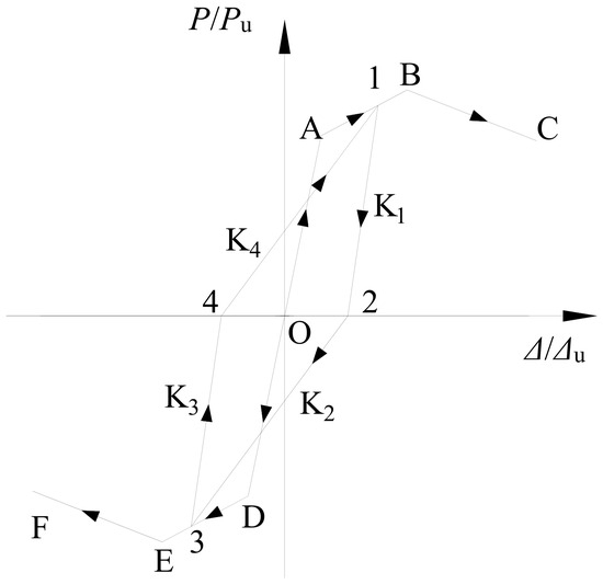
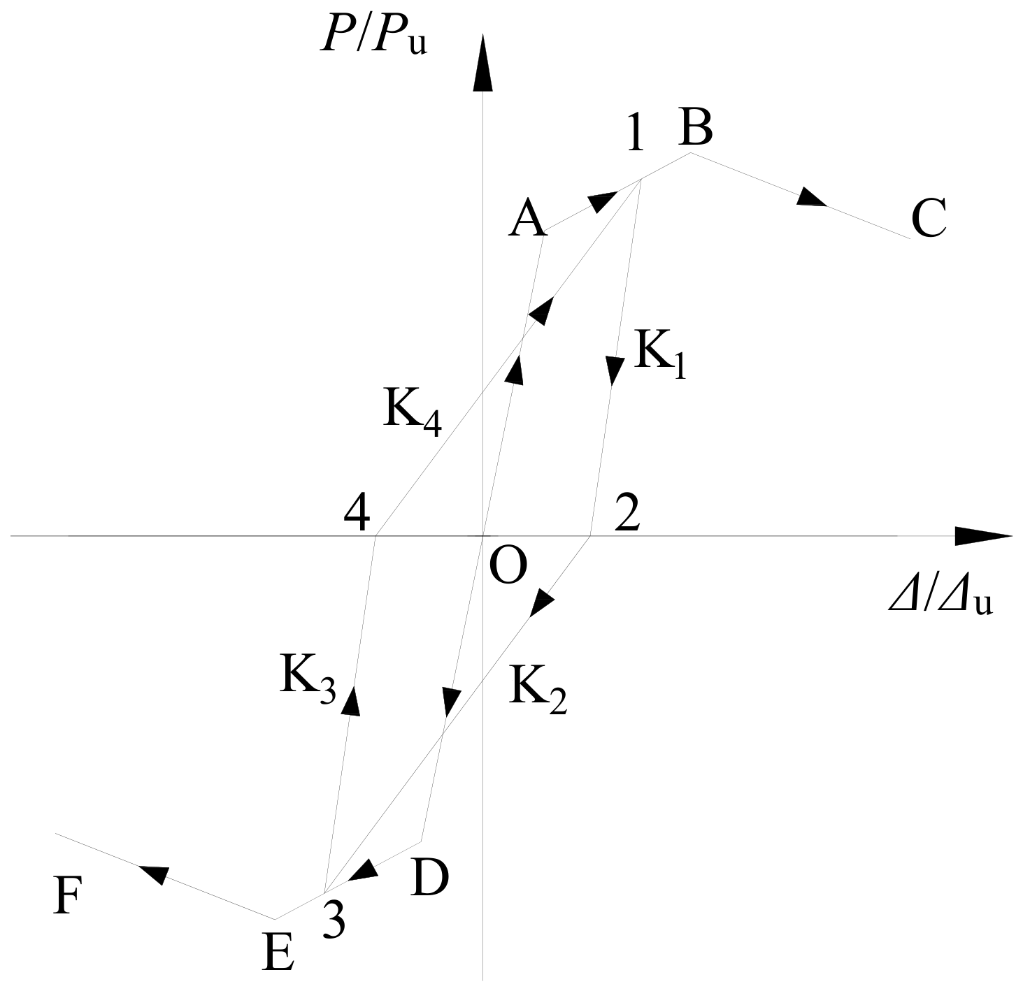
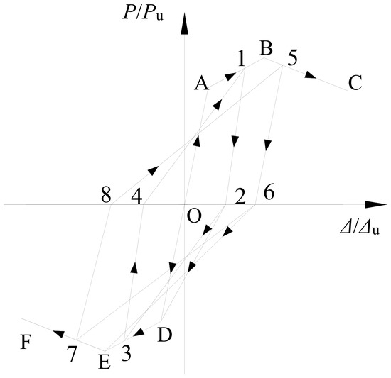
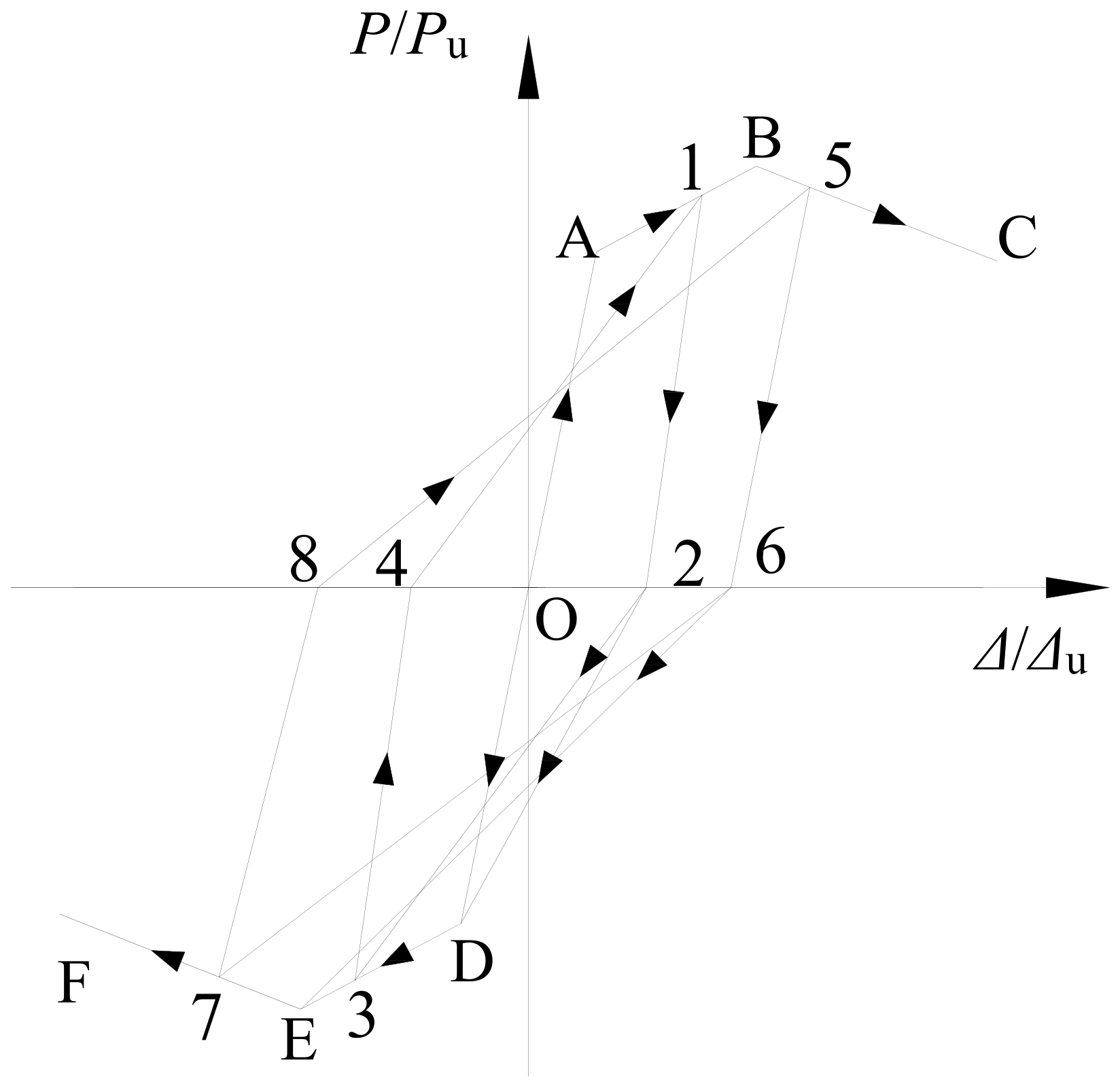
Based on the three-segment backbone curve model, stiffness degradation relationships, and cyclic loading path rules, the restoring force model shown in Figure 20 was established. Before yielding, the unloading path coincided approximately with the initial loading path, and the unloading stiffness was assumed to be equal to the initial stiffness. After yielding, the positive and negative unloading stiffnesses were determined using Equations (4) and (6), respectively, while the positive and negative reloading stiffnesses were calculated using Equations (5) and (7), respectively.
Figure 20.
Restoring force model.
During reverse loading, the loading path first pointed toward the previously experienced maximum deformation point in the corresponding loading direction. Once the reloading path intersected with the backbone curve, the response continued along the corresponding backbone curve until the next unloading stage occurred. The same loading and unloading rules were subsequently applied to the following loading cycles.
For clarity, the step-by-step calculation procedure of the proposed restoring force model is summarized as follows:
(1) Prescribe the displacement Δi at the current loading step and determine the loading direction according to Δi − Δi−1.
(2) Determine whether the current response follows the skeleton curve, unloading branch, or reverse reloading branch according to the loading history and the previously reached maximum positive and negative displacements.
(3) When a new maximum displacement is reached, calculate the corresponding load Pi from the appropriate segment of the positive or negative skeleton curve.
(4) When unloading occurs, calculate Pi using the corresponding unloading stiffness K1 or K3 and the coordinates of the unloading point.
(5) After load reversal, determine the target historical maximum deformation point in the opposite loading direction and calculate Pi along the corresponding reloading branch.
(6) When the reloading path reaches the prescribed historical point or intersects the skeleton curve, switch to the corresponding subsequent branch according to the hysteretic rules shown in Figure 20.
(7) Update Pi, Δi, the loading direction, and the historical maximum positive and negative displacements, and repeat Steps (1)–(6) for the next displacement increment.
As an illustrative example, the first 55 mm loading cycle of specimen DBJ-V88 is considered. At Δ = 55 mm, the response is located on the positive post-peak branch of the skeleton curve, giving P = 96.36 kN. During unloading, the calculated unloading stiffness is K1 = 2.5435 kN/mm, resulting in a zero-load point of Δ = (17.12 mm,0). During reverse loading, the path is directed toward the previously reached negative maximum displacement point (−42 mm, −90.89 kN), and subsequently reaches (−55, −91.95 kN) along the negative skeleton curve. The negative unloading stiffness is then calculated as K3 = 2.1727 kN/mm, giving the second zero-load point (−12.68 mm, 0). The subsequent positive reloading branch is directed toward the previous positive maximum deformation point (42 mm, 94.58 kN). The state variables are then updated, and the same procedure is repeated for the next displacement increment.
4.4. Model Validation
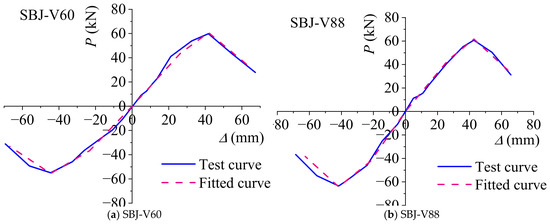
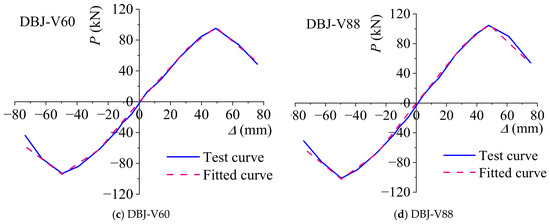
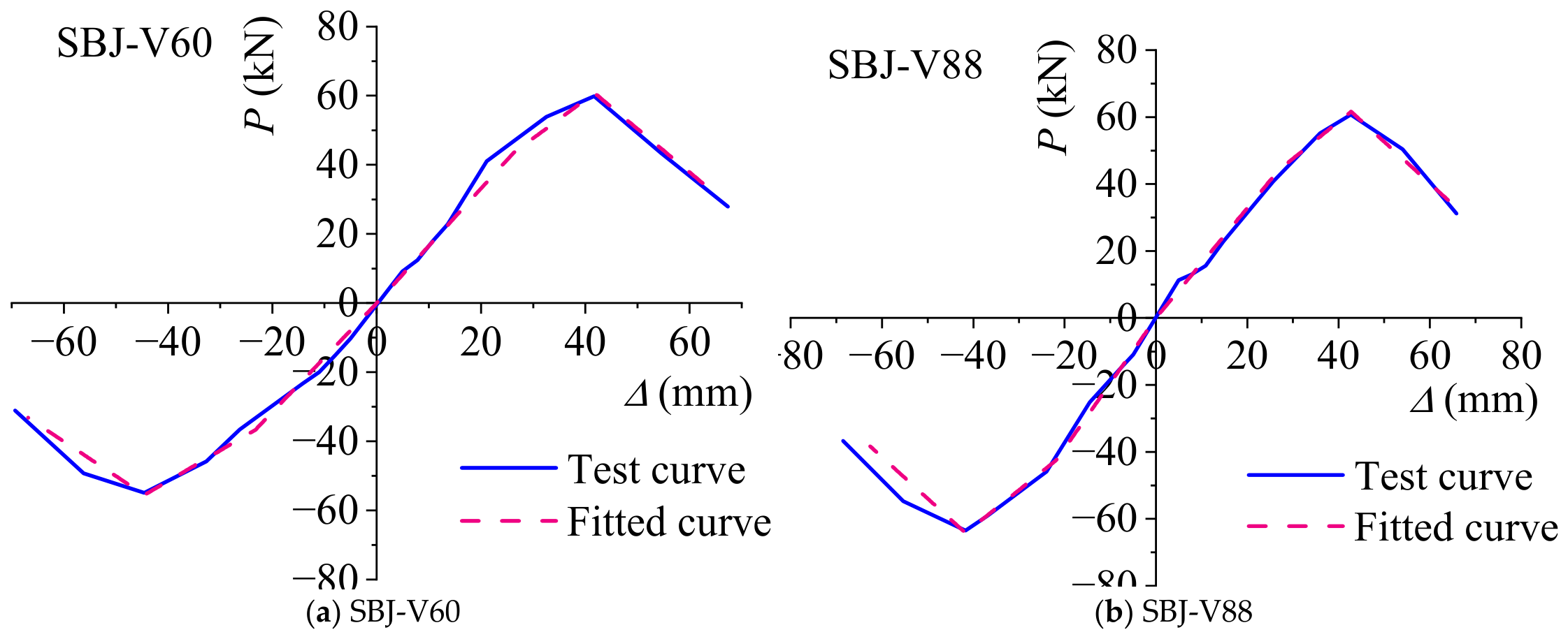
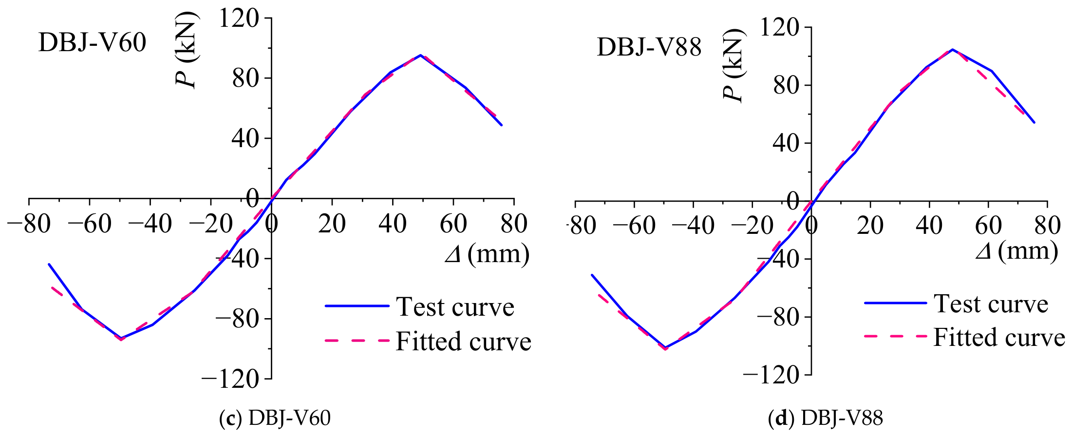
Using the proposed three-segment backbone curve model, the load–displacement backbone curves of SBJ-V60, SBJ-V88, DBJ-V60, and DBJ-V88 specimens were calculated and compared with the experimental results, as shown in Figure 21.
Figure 21.
Comparison between experimental and predicted backbone curves of specimens.
As shown in Figure 21, the proposed three-segment model can reasonably capture the overall evolution characteristics of the backbone curves of all four specimens. The calculated results accurately represent the initial elastic stiffness, post-yield strengthening behavior, peak load capacity, and post-peak degradation characteristics. For specimens with different beam–column configurations and viscous damper parameters, the predicted curves show good agreement with the experimental results around the yield points, peak points, and failure points. This indicates that the normalized backbone curve approach and unified parameter identification method can effectively describe the nonlinear load-carrying characteristics of different viscous damper-equipped joints.
Good agreement between the model predictions and experimental results was observed during the elastic and strengthening stages. Some deviations occurred in the post-peak degradation stage, which can be attributed to the randomness of local buckling, crack initiation, and crack propagation at the beam ends. In addition, the three-segment model simplifies the complex damage evolution process by adopting an equivalent linear degradation branch. Nevertheless, the proposed model can effectively capture the main deformation stages and degradation trend of the joint response.
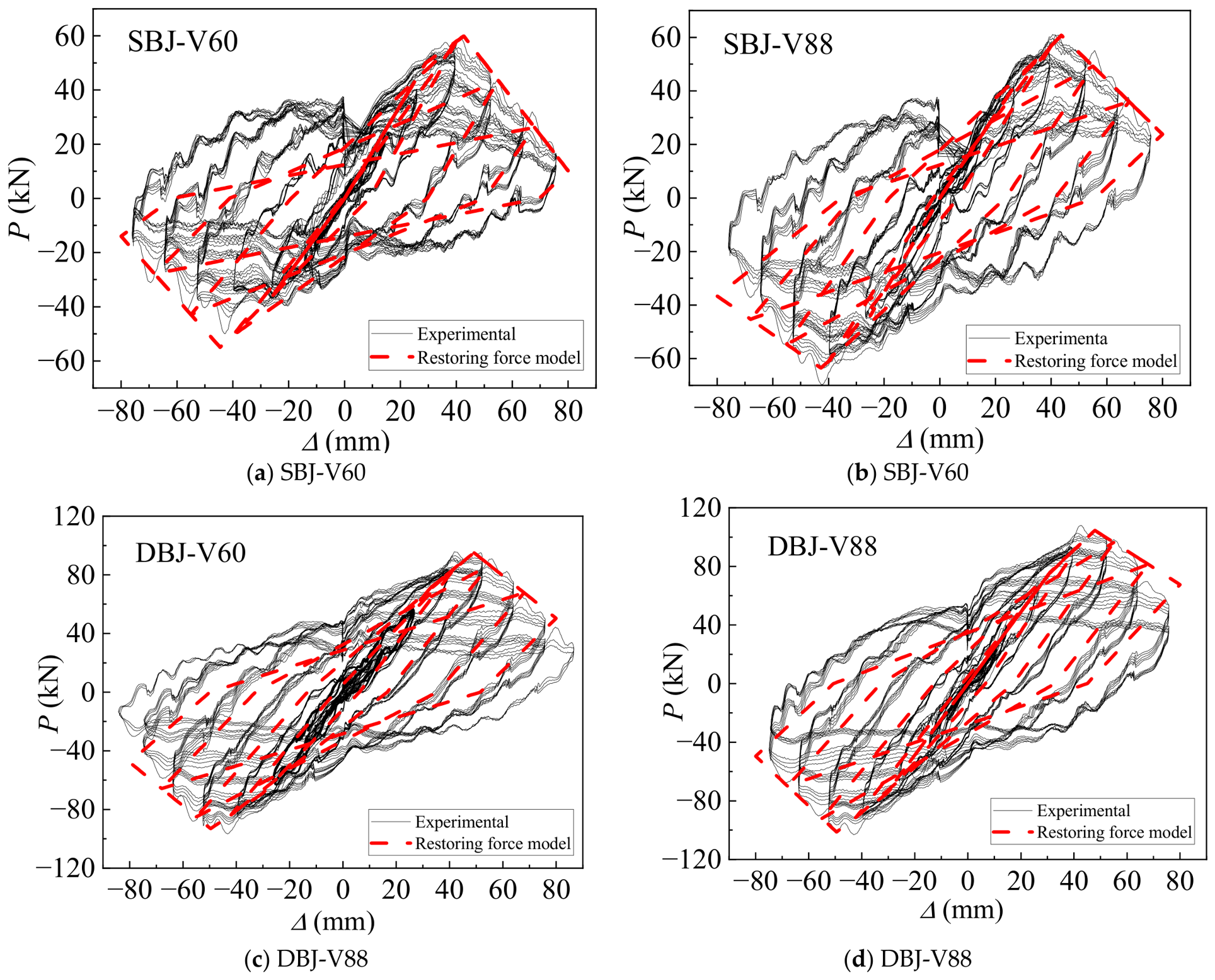
To further evaluate the capability of the proposed restoring force model in reproducing the complete cyclic response, representative loading cases after the specimens approached or entered the yielding stage were selected for comparison with the experimental hysteretic curves. Cases 9, 11, 13, 15, and 17 were considered, corresponding to progressively increasing displacement amplitudes. The pre-yield loading cases were not separately plotted because the model assumes that the unloading path coincides with the initial loading path before yielding. These loading cases were used as additional validation cases for the complete hysteretic response, rather than for identifying the backbone-curve parameters.
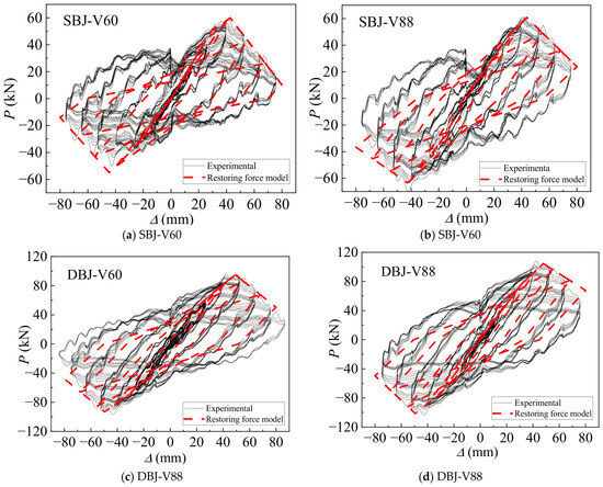
Figure 22 compares the calculated hysteretic responses with the experimental results for the four specimens. Although local differences exist between the calculated and experimental curves, particularly at large deformation levels, the proposed model reasonably reproduces the overall hysteretic shape, the positive and negative peak responses, the degradation of unloading and reloading stiffness, and the evolution of the cyclic response with increasing displacement amplitude. The discrepancies at large deformation levels are mainly associated with local buckling, crack propagation, and accumulated plastic damage at the beam ends, which cannot be fully represented by the simplified restoring force rules.
Figure 22.
Comparison between experimental and calculated hysteretic responses of the specimens.
Overall, the proposed restoring force model can provide a unified description of the nonlinear response characteristics of steel archaizing building joints equipped with viscous dampers. The cyclic behavior of the joints is reproduced by incorporating the unloading and reloading stiffness degradation relationships in both positive and negative loading directions. The proposed model has a relatively simple form, and all required parameters can be determined from the experimentally obtained yield points, ultimate points, failure points, and stiffness degradation characteristics. Therefore, within the range of the present tests, the proposed model provides a practical approach for nonlinear seismic response analysis of steel archaizing building joints equipped with viscous dampers.
5. Conclusions
Based on the dynamic cyclic loading tests and restoring force modeling of four steel archaizing building beam–column joints equipped with viscous dampers, the following conclusions can be drawn:
(1) The failure of all specimens was concentrated in the beam-end plastic hinge regions. With increasing displacement amplitudes, local buckling occurred in the beam flanges and webs, followed by base metal tearing within the plastic hinge regions. No obvious yielding was observed in the columns or joint core regions, indicating that the designed specimens achieved the expected beam-controlled failure mode.
(2) All four specimens exhibited stable and spindle-shaped hysteretic loops without obvious pinching behavior. The specimens showed typical nonlinear responses, including elastic response, yielding, stiffness degradation, and strength deterioration. The displacement ductility coefficients ranged from 1.77 to 2.05, indicating that the viscous damper-equipped joints possessed satisfactory deformation capacity under dynamic cyclic loading.
(3) The skeleton curves of the specimens exhibited three distinct stages, including the elastic stage, the post-yield strengthening stage, and the post-peak degradation stage. The ultimate loads of the four specimens ranged from 59.88 kN to 104.55 kN, while the corresponding failure displacements ranged from 52.63 mm to 61.50 mm. The experimental skeleton curves provided the basis for establishing the trilinear skeleton curve model.
(4) With increasing displacement amplitudes and cumulative cyclic damage, both unloading and reloading stiffness gradually decreased. The stiffness degradation relationships obtained through regression analysis reasonably described the variation trends of unloading and reloading stiffness during cyclic loading.
(5) Based on the experimental skeleton curves, stiffness degradation characteristics, and hysteretic responses, a restoring force model was developed for steel archaizing building beam–column joints equipped with viscous dampers. The proposed model incorporates a trilinear skeleton curve, stiffness degradation relationships, and hysteretic rules. Comparisons with the experimental hysteretic curves show that the model reasonably reproduces the main hysteretic characteristics, including the overall loop shape, peak responses, and stiffness degradation. Within the range of the present tests, the proposed model can be used for nonlinear dynamic analysis of this type of joint.
The scientific significance of this study lies in introducing viscous dampers into the Que-ti bracket region of steel archaizing building joints and establishing a corresponding dynamic testing and restoring force modeling approach. The proposed configuration combines the architectural constraints of archaizing buildings with supplemental energy dissipation, while the restoring force model provides a simplified description of the skeleton response, stiffness degradation, and cyclic hysteretic behavior of this type of joint. These results provide an experimental and analytical basis for further seismic response analysis of viscous damper-equipped steel archaizing buildings. From an engineering perspective, the Que-ti bracket region provides a feasible location for installing viscous dampers while preserving the traditional architectural appearance.
In practical design, the damper parameters should be determined according to the geometric constraints of the joint, the expected deformation and velocity demands, and the target energy dissipation requirements of the specific structure. Future studies will focus on smaller viscous dampers better suited to the dimensional constraints of steel archaizing joints, as well as other energy-dissipation devices such as shape memory alloy dampers, to further promote their application in practical engineering.
Author Contributions
Conceptualization, Z.W.; methodology, J.D.; writing—original draft preparation, Z.W. and L.Z.; writing—review and editing, L.Z. and M.C.; software, J.D.; supervision, H.S. and J.D.; project administration, H.S.; funding acquisition, L.Z. All authors have read and agreed to the published version of the manuscript.
Funding
This work was supported by the National Natural Science Foundation of China (Grant No. 52008330), the Natural Science Foundation of Henan Province (Grant No. 252300421260), and the Joint Fund for Science and Technology Research Projects of Henan Province (Grant No. 252103810049). This work was also supported by the Major Science and Technology Program of Hainan Province (Grant No. ZDKJ201803) and the Postgraduate Education Reform and Quality Improvement Project of Henan Province (Grant Nos. YJS2025YBGZZ50 and YJS2026YBGZZ53).
Data Availability Statement
The original contributions presented in this study are included in the article. Further inquiries can be directed to the corresponding author.
Conflicts of Interest
Author Lin Zhang was employed by Shanghai Municipal Engineering Design Institute (Group) Co., Ltd. The remaining authors declare that the research was conducted in the absence of any commercial or financial relationships that could be construed as a potential conflict of interest.
References
- Zhang, X.; Liu, L.; Cui, L.; Liu, K.; Li, J. Nonlinear dynamic analysis of ancient timber structures with rotary friction dampers. J. Build. Eng. 2025, 100, 111707. [Google Scholar] [CrossRef] [Scilit]
- Qi, L.J.; Cao, Y.; Xue, J.Y.; Yuan, Z.; Ling, H.Q.; Meng, R.F. Seismic performance evaluation and engineering application of modern Chinese traditional-style buildings: State-of-the-art review. Structures 2023, 56, 105022. [Google Scholar] [CrossRef] [Scilit]
- Qi, L.J.; Xue, J.Y.; Leon, R.T. Experimental and analytical investigation of transition steel connections in traditional-style buildings. Eng. Struct. 2017, 150, 438–450. [Google Scholar] [CrossRef] [Scilit]
- Qi, L.J.; Xue, J.Y. Pseudo-dynamic test and time-history analyses of traditional-style steel frame structures. Int. J. Steel Struct. 2018, 18, 402–416. [Google Scholar] [CrossRef] [Scilit]
- Xue, J.Y.; Qi, L.J.; Yang, K.; Wu, Z.J. Dynamic experimental study on single- and double-beam column joints in steel traditional-style buildings. Struct. Eng. Mech. 2017, 63, 617–628. [Google Scholar]
- Xue, J.Y.; Ma, L.L.; Wu, Z.J. Seismic performance of steel joints between double beams and columns in Chinese traditional-style buildings. Int. J. Steel Struct. 2018, 18, 417–432. [Google Scholar] [CrossRef] [Scilit]
- Yuan, Z.; Qi, L.J.; Xue, J.Y. Seismic performance of steel semi-rigid friction-damped joints with replaceable angles in modern Chinese traditional-style buildings. J. Constr. Steel Res. 2023, 207, 107948. [Google Scholar] [CrossRef] [Scilit]
- Yuan, Z.; Qi, L.J.; Xue, G.M.; Xue, J.Y. Resilient joints with SMA bar-shear friction damper devices in modern Chinese traditional-style steel buildings: Seismic performance evaluation and optimized design. J. Build. Eng. 2024, 82, 108300. [Google Scholar] [CrossRef] [Scilit]
- Qi, L.J.; Yuan, Z.; Xue, J.Y. Experimental and numerical study on seismic performance of steel semi-rigid joints equipped with SMA bars and friction dampers. Eng. Struct. 2024, 301, 117320. [Google Scholar] [CrossRef] [Scilit]
- Qi, L.J.; Xue, J.Y.; Sui, Y.; Wu, Z.J. Smart retrofitting of irregular steel joints in traditional Chinese buildings using viscous dampers. Eng. Struct. 2021, 228, 111526. [Google Scholar] [CrossRef] [Scilit]
- Torres-Rodas, P.; Zareian, F.; Kanvinde, A. Hysteretic model for exposed column-base connections. J. Struct. Eng. 2016, 142, 04016102. [Google Scholar] [CrossRef] [Scilit]
- Zheng, H.D.; Fan, J. Phenomenological hysteretic model for steel braces including inelastic postbuckling and low-cycle fatigue prediction. J. Struct. Eng. 2019, 145, 04019037. [Google Scholar] [CrossRef] [Scilit]
- Elkady, A.; Lignos, D.G. Improved seismic design and nonlinear modeling recommendations for wide-flange steel columns. J. Struct. Eng. 2018, 144, 04018149. [Google Scholar] [CrossRef] [Scilit]
- Abdollahzadeh, G.; Shabanian, S.M. Experimental and numerical analysis of beam to column joints in steel structures. Front. Struct. Civ. Eng. 2018, 12, 642–661. [Google Scholar] [CrossRef] [Scilit]
- Žarković, D.; Jovanović, Đ.; Vukobratović, V. A new constitutive model for beam-to-column connections of steel storage racks. Thin-Walled Struct. 2018, 127, 295–302. [Google Scholar] [CrossRef] [Scilit]
- Wu, C.L.; Liu, X.; Pan, W.; Mou, B. Restoring force model for steel beam to CFST/HSS column joints with a reinforced concrete slab. J. Build. Eng. 2023, 73, 106688. [Google Scholar] [CrossRef] [Scilit]
- Nie, S.; Long, H.; Ye, X.; Deng, Y.; Chen, Z.; Ma, C.; Pan, J. Hysteretic behavior and restoring force model of Q960 high-strength steel tapered reduced beam-column joints. J. Chongqing Univ. 2025, 48, 81–93. [Google Scholar]
- Ibarra, L.F.; Medina, R.A.; Krawinkler, H. Hysteretic models that incorporate strength and stiffness deterioration. Earthq. Eng. Struct. Dyn. 2005, 34, 1489–1511. [Google Scholar] [CrossRef] [Scilit]
- Lignos, D.G.; Krawinkler, H. Deterioration modeling of steel components in support of collapse prediction of steel moment frames under earthquake loading. J. Struct. Eng. 2011, 137, 1291–1302. [Google Scholar] [CrossRef] [Scilit]
- Dong, J.S.; Gong, Y.R.; Xue, J.Y.; Sui, Y.; Huang, B. Experimental research on Chinese antique buildings with dual lintel-column joints of steel and composite structures. J. Asian Archit. Build. Eng. 2024, 23, 698–711. [Google Scholar] [CrossRef] [Scilit]
- Li, J. The Construction Method; Commercial Press: Shanghai, China, 1932. [Google Scholar]
- GB 50661-2011; Code for Welding of Steel Structures. China Architecture & Building Press: Beijing, China, 2011.
- GB 50017-2017; Standard for Design of Steel Structures. Ministry of Housing and Urban-Rural Development of the People’s Republic of China: Beijing, China, 2017.
- GB/T 2975-2018; Steel and Steel Products—Location and Preparation of Samples and Test Pieces for Mechanical Testing. Chinese Standard Press: Beijing, China, 2018.
- GB/T 228.1-2021; Metallic Materials—Tensile Testing—Part 1: Method of Test at Room Temperature. Standardization Administration of the People’s Republic of China: Beijing, China, 2021.
- JGJ/T 101-2015; Specification for Seismic Test of Buildings. China Architecture & Building Press: Beijing, China, 2015.
- JG/T 209-2012; Dampers for Vibration Energy Dissipation of Buildings. China Architecture & Building Press: Beijing, China, 2012.
- JT/T 926-2014; Fluid Viscous Dampers for Bridges. China Communications Press: Beijing, China, 2014.
- Japan Society of Seismic Isolation (JSSI). Passive Damping Structure Design and Construction Manual; Japan Society of Seismic Isolation: Tokyo, Japan, 2013. [Google Scholar]
- ASCE/SEI 41-23; Seismic Evaluation and Retrofit of Existing Buildings. American Society of Civil Engineers: Reston, VA, USA, 2023.
- JGJ 297-2013; Technical Specification for Energy Dissipation and Vibration Reduction of Buildings. China Architecture & Building Press: Beijing, China, 2013.
- Chung, T.S.; Lam, E.S.; Wu, B.; Xu, Y. Retrofitting reinforced concrete beam-column joints by hydraulic displacement amplification damping system. In Proceedings of the Structures Congress 2007, Long Beach, CA, USA, 16–19 May 2007. [Google Scholar]
- Liu, W.Q.; Ge, W.; Lu, W.D. Experimental study on seismic behavior of energy-dissipated braced frame structures with concrete-filled rectangular steel tubular columns and steel beams. Earthq. Eng. Eng. Vib. 2004, 24, 106–109. [Google Scholar]
- GB/T 17742-2020; Chinese Seismic Intensity Scale. China Architecture & Building Press: Beijing, China, 2020.
- Palanci, M. Flexural Response Prediction of Reinforced Concrete Members Based on Statistical Observations. Arab. J. Sci. Eng. 2017, 42, 3689–3709. [Google Scholar] [CrossRef] [Scilit]

Disclaimer/Publisher’s Note: The statements, opinions and data contained in all publications are solely those of the individual author(s) and contributor(s) and not of MDPI and/or the editor(s). MDPI and/or the editor(s) disclaim responsibility for any injury to people or property resulting from any ideas, methods, instructions or products referred to in the content. |
© 2026 by the authors. Licensee MDPI, Basel, Switzerland. This article is an open access article distributed under the terms and conditions of the Creative Commons Attribution (CC BY) license.