


Abstract
The progressive development of 3D subsurface geotechnical maps requires integrating site-based voxel models produced from neighboring engineering-geological investigations, but directly joining separately interpolated classified voxel models can produce artificial boundary discontinuities. This study proposes a GIS-based workflow for reducing such discontinuities through Empirical Bayesian Kriging 3D (EBK 3D) re-interpolation, tested on two adjacent construction sites in Astana, Kazakhstan. Separate 1 × 1 × 1 m classified voxel models were generated for Site A and Site B and compared at their boundary using face-to-face and 1 m offset schemes. Before re-interpolation, the face-to-face boundary matching ratio (BMR) was 49.4%, and the boundary discontinuity ratio (BDR) was 50.6%. Two alternative re-interpolation strategies were then tested: joint-raw EBK 3D interpolation applied directly to the pooled borehole data, and a two-step approach joining and re-interpolating the previously interpolated per-site voxel tables. Both substantially improved face-to-face continuity (BMR rising to 99.1% for joint-raw and 95.7% for the two-step approach), but the two-step approach produced a considerably larger improvement in the surrounding offset neighborhood (BMR increasing to 74.8%, versus 56.9% for joint-raw), indicating it extends greater numerical continuity beyond the immediate contact layer. The two-step approach, used as the primary method, achieved a combined soil-type preservation ratio of 85.9% (88.3% for Site A, 82.7% for Site B). These results demonstrate improved numerical and visual interface continuity rather than independently validated geological accuracy; engineering application would require independent validation and uncertainty quantification. The approach supports the transition from isolated site-scale voxel models toward an expandable 3D subsurface geotechnical mapping system.
1. Introduction
Reliable interpretation of subsurface conditions is essential for safe and economical design of buildings, infrastructure, underground facilities, and urban development projects. Engineering-geological surveys usually provide direct information about soil stratification and geotechnical properties through boreholes, laboratory tests, in situ tests, and, in some cases, geophysical investigations. However, these data are spatially discrete and often insufficient for representing the continuous lateral and vertical variability of subsurface conditions. This limitation becomes especially important in urban areas, where ground conditions may vary over short distances and where incomplete interpretation of soil stratification can increase design uncertainty, construction risks, and the probability of unexpected ground behavior. In Kazakhstan, the need for GIS-based special geotechnical mapping has also been emphasized because such maps can support the assessment of construction-ground conditions and the solution of practical foundation-design and urban-planning tasks, although their implementation in engineering practice remains limited [1]. Marache et al. [2] emphasized that city-scale geotechnical models are needed because urban planning and infrastructure development require preliminary knowledge of underground lithological and mechanical conditions. Dong et al. [3] similarly noted that three-dimensional (3D) engineering-geological and geotechnical models are useful for reducing uncertainty in shallow urban subsurface interpretation and for supporting engineering decisions. He et al. [4] also showed that 3D geological models of shallow subsurface conditions can support urban underground space development by visualizing stratigraphic geometry and geotechnical property variation.
3D geological and geotechnical modeling has therefore become an important tool for transforming discrete site investigation data into continuous spatial representations of the subsurface. Compared with traditional two-dimensional (2D) maps and cross-sections, 3D models allow soil layers, engineering-geological units, and geotechnical parameters to be visualized and analyzed within their actual spatial context. Petrone et al. [5] demonstrated that 3D engineering-geological modeling can support the definition of engineering-geological units by combining lithological, stratigraphic, and geotechnical information. Zhu et al. [6] further highlighted that large-scale urban 3D geological modeling requires the integration of multi-source heterogeneous data and appropriate modeling schemes to avoid excessive generalization of geological information. These studies confirm that 3D subsurface models are increasingly required not only for visualization, but also for practical engineering interpretation, spatial analysis, and decision support.
Geostatistical methods are widely used in 3D subsurface modeling because they account for spatial dependence and provide a basis for estimating values at unsampled locations. Kim et al. [7] proposed a 3D geotechnical spatial modeling method based on borehole data and optimized geostatistical approaches, using Ordinary Kriging and conditional simulation to model subsurface stratification and SPT-N values. Kim et al. [8] later developed a geostatistical optimization model for mapping subsurface stratification and SPT-N values at a dam site by integrating borehole and geophysical data and comparing interpolation reliability through cross-validation. Han et al. [9] also demonstrated the value of geostatistical-learning-based integration of borehole logs and geophysical data for site-specific 3D stratigraphic prediction in an urban area. These studies show that geostatistical interpolation can improve the reliability of subsurface interpretation when compared with purely discrete borehole-based descriptions. Nevertheless, most such frameworks are still focused on producing a complete model for one project area or one predefined modeling domain.
Voxel-based modeling is particularly suitable for 3D subsurface representation because it divides the underground space into volumetric cells that can store lithological, geotechnical, or classification attributes. Nonogaki et al. [10] proposed a voxel modeling method for geotechnical characteristics in an urban area using a large number of borehole logs and Natural Neighbor interpolation, showing that voxel models can provide an objective overview of lithofacies and SPT-N distributions. Enemark et al. [11] compared layer-based and voxel-based geological modeling strategies and showed that the choice of geological model structure can influence subsequent groundwater modeling results, confirming that voxel models are not only visualization objects but also analytical inputs that affect downstream predictions. Khan et al. [12] developed a BIM–GIS geological data management system using both boundary and voxel representations, showing that voxel models can represent inhomogeneous geological information, support spatial queries, and be updated at different scales. Li et al. [13] also proposed a regular voxel splitting method for 3D geological implicit modeling, emphasizing that voxel-based structures can support internal information representation and web-based visualization of geological bodies. Together, these studies show that voxel models are useful for managing complex and spatially variable subsurface data, especially when volumetric representation and attribute-based analysis are required.
Recent developments have also expanded 3D geological and geotechnical modeling through machine learning, neural networks, and hybrid data-driven approaches. Jia et al. [14] used a Stacking machine learning methodology to classify and predict rock types for 3D geological modeling from geological and geophysical datasets. Li et al. [15] proposed a progressive geological modeling strategy using machine learning and uncertainty analysis, showing that classification-based modeling can integrate stratigraphic and lithological information. Guo et al. [16] introduced a Semi-supervised deep learning method using pseudo-labels for shallow strata modeling from borehole data in urban areas, addressing the problem of limited training data. Hillier et al. [17] and Hillier et al. [18] further demonstrated the potential of graph neural networks and implicit neural representations for 3D structural geological modeling. Although these approaches are promising, they usually require either specialized data structures, training strategies, or larger datasets than are typically available in routine engineering-geological surveys. For construction-site datasets with limited borehole and laboratory information, geostatistical GIS-based workflows may remain more practical because they can be applied directly to standard geotechnical tables, as demonstrated in previous EBK 3D voxel-based geotechnical modeling [19].
For engineering-geological applications, one of the important tasks is not only to interpolate individual geotechnical parameters, but also to classify the soil type or engineering-geological unit in each part of the modeled subsurface. Vessia et al. [20] used geostatistical data fusion of CPT parameters to model 3D soil lithotype variability and geotechnical properties, demonstrating the value of combining geotechnical measurements and spatial interpolation for litho-technical characterization. Song and Tsai [21] proposed Interval Kriging for 3D lithofacies modeling from borehole data and showed that borehole intervals can be used efficiently to reproduce lithofacies architecture and spatial connectivity. Utepov et al. [19] developed a voxel-based geoprocessing workflow using Empirical Bayesian Kriging 3D (EBK 3D) and a Best-Fit Convergence Function (BFCF) to interpolate geotechnical properties and assign soil types to 1 × 1 × 1 m voxels. That study demonstrated that classified voxel models can reveal subsurface soil stratification and store geotechnical property information at each voxel position. However, the workflow was applied to an individual construction site and did not address how separately generated classified voxel models from neighboring sites can be integrated into a continuous subsurface cartographic system. This issue becomes important when 3D subsurface mapping is considered not as a one-time model for a single construction site, but as a progressively expandable geotechnical cartographic database. In practice, engineering-geological surveys are usually performed site by site, following the boundaries of individual construction projects. As a result, separate voxel models can be generated for adjacent sites, but direct placement or merging of these models may produce artificial discontinuities at their common boundary [22]. These discontinuities may appear because each model is interpolated independently, with its own borehole configuration, interpolation extent, and edge effects. Even when the geological environment is generally similar, soil layers classified in one model may not align with the corresponding layers in the neighboring model. Existing studies have addressed 3D subsurface interpolation, multi-source integration, voxel data management, and uncertainty analysis, but the specific problem of joining neighboring classified voxel models and improving soil-layer continuity across their interface has received limited attention, a gap also noted in a recent review of 3D subsurface cartography approaches for geotechnical ground characterization [22]. Moreover, it remains unclear how far re-interpolation should be repeated after joining neighboring voxel models, because additional interpolation cycles may improve apparent continuity but may also increase smoothing and reduce preservation of the original soil-type pattern.
The need to address this problem is also related to the general limitations of spatial interpolation and grid-based modeling. Dong et al. [3] noted that uncertainty in 3D geological and geotechnical models is strongly affected by data density, geological complexity, and interpolation quality. Nonogaki et al. [10] emphasized that voxel modeling should remain objective and practical, but the resulting model still depends on the interpolation scheme and the spatial distribution of borehole data. Khan et al. [12] pointed out that voxel size is a key factor controlling the representation of complex geological features, while Enemark et al. [11] showed that voxel and layer modeling strategies can lead to different model outputs even when based on the same geological conceptualization. These observations imply that when two neighboring voxel models are generated separately, their boundaries may contain modeling artifacts that reflect the modeling procedure rather than true geological discontinuities. Therefore, a methodological solution is needed to integrate neighboring voxel models while preserving the general stratification pattern and reducing artificial boundary mismatch.
The present study addresses this gap by proposing a workflow for reducing boundary discontinuities in voxel-based subsurface geotechnical mapping through EBK 3D re-interpolation. The study extends the voxel-based EBK 3D classification framework of [19] from isolated site-scale modeling toward stepwise integration of neighboring subsurface models. The study aims to develop and evaluate a GIS-based geoprocessing workflow for improving soil-layer continuity when neighboring classified subsurface voxel models are joined. The specific objectives are: (i) to generate separate classified voxel models for two adjacent construction sites using EBK 3D interpolation and soil-type classification; (ii) to quantify the degree of soil-type matching and discontinuity at their common boundary; (iii) to perform EBK 3D re-interpolation using the joined voxel attribute data; and (iv) to evaluate whether the resulting joint classified voxel model improves direct boundary continuity while preserving the general soil-type composition. The proposed workflow is intended to support the gradual development of expandable 3D voxel-based subsurface geotechnical maps as new engineering-geological data become available from nearby construction sites.
2. Materials and Methods
2.1. Study Area and Input Geotechnical Data
The study was conducted for two neighboring construction sites located in Astana, Kazakhstan. The source data were obtained from engineering-geological surveys carried out by Guzyr [23]. The two sites are located close to each other and share a common interface, which makes them suitable for testing the proposed voxel-model joining and re-interpolation workflow. Site A (outlined in blue) is located on the left side of the study area, and Site B (outlined in burgundy) on the right; dotted line in Figure 1 shows the common interface between them. Site A includes 17 boreholes and 49 samples (Table A1), while Site B includes 18 boreholes and 50 samples (Table A2). The spatial arrangement of the boreholes and the relative position of the two site borders are presented in Figure 1 using the geographical coordinates (i.e., longitude and latitude).
Figure 1.
Location of construction sites A and B, borehole positions, site borders, and common interface (adopted from [23]).
The engineering-geological data (Appendix A) used in this study include borehole number, sampling depth, spatial coordinates, and geotechnical properties (a mix of directly measured laboratory values and, where individual test data were unavailable, EGE-level normative values from the original survey report). Direct inspection of Appendix A confirms this: 21 of the 99 records (21.2%) share identical cohesion, friction angle, deformation modulus, void ratio, and moisture-content values with at least one other record from a different borehole, which is characteristic of EGE-level normative values applied uniformly within a layer rather than independent per-sample laboratory results; this reflects standard practice in the original geotechnical survey report [23], where not every sampling depth within an EGE necessarily received a full independent laboratory test battery. The input parameters used for voxel interpolation were cohesion [kPa], internal friction angle [°], deformation modulus [MPa], plasticity index [%], liquidity index , void ratio , natural moisture content [%], particle size [mm], and particle size distribution [%]. These parameters were prepared in a unified tabular format for automated processing in ArcGIS Pro 3.5 (Esri Inc., Redlands, CA, USA). The “sampling depth” recorded for each entry in Appendix A represents the depth at which a discrete soil sample was extracted and tested within a given EGE layer (typically near the layer’s midpoint, following standard geotechnical sampling practice), not the full vertical interval occupied by that EGE. The EGE layer thickness intervals themselves (the depth ranges over which each engineering-geological element extends) are documented in the original geotechnical survey report [23] but were not reproduced in Appendix A, since the voxel interpolation and classification workflow operates on point-located property values rather than on interval-averaged layer properties; this is consistent with the borehole-log stratigraphic diagrams typically used for visual EGE characterization, but is a distinct representation from the point data used here for spatial interpolation.
The choice to interpolate from discrete sample depths rather than from the full EGE interval thicknesses reflects what the underlying data actually support: EGE boundaries are qualitative lithological classifications assigned by field logging, while the nine quantitative geotechnical properties used for interpolation and classification (Section 2.2) are measured only at discrete sample depths within each interval, typically near its midpoint. Treating an entire EGE interval as carrying a single constant property value, rather than the point-sampled value, would not add genuine information about within-layer property variation, since no additional measurements exist within most intervals to support such variation; it would instead extend the existing normative-value pattern already present in part of the dataset (Section 2.1) across every voxel within that interval, at the cost of removing the point-specific character of the available measurements. It would also not change how properties are estimated between boreholes, since spatial interpolation, not within-borehole interval assignment, is what determines voxel values away from sampled locations. A more direct comparison between predicted voxel classes and observed borehole stratigraphy is reported separately in Section 3.2.2, where classification-level leave-one-borehole-out cross-validation compares soil types predicted from neighboring boreholes against soil types classified directly from each withheld borehole’s own measured properties.
The same structure was used for both sites to ensure compatibility during the subsequent joining of voxel attribute tables.
The soil stratification of the two sites was represented through engineering-geological elements (EGEs), which were retrieved from the borehole descriptions and laboratory data. According to Appendix A, Site A contains several major EGEs, including light sandy loams with interbeds and lenses of heavy silty loam, sandy loams, medium-grained sands, gravelly sands, gravel soils with sand inclusions, and interbedded light sandy loams and light silty loams with rare lenses of sandy loams. The Site A data include samples from different boreholes and depths, with the values of , , , , , , , and recorded for each sampling interval (Appendix A, Table A1). Site B has a similar but not identical EGE structure, including light sandy loams with interbeds and lenses of heavy sandy loams and light silty loams, sandy loams, medium-grained sands, coarse sands, gravelly sands, gravel soils with sand inclusions, and interbedded sandy loams and silty loams (Appendix A, Table A2). This similarity of the general soil profile, combined with local differences in EGE occurrence, provides an appropriate basis for testing whether re-interpolation can improve the continuity of the classified voxel model across the site interface.
It should be noted that the EGE numbering is not a unified stratigraphic correlation scheme across the two sites. Site A’s EGE 1 combines light sandy loam with heavy silty loam interbeds, whereas Site B’s EGE 1 combines light sandy loam with heavy sandy loam interbeds—a different lithological pairing under the same EGE index. Site A’s EGE sequence has no EGE 4 (jumping from EGE 3 to EGE 5), while Site B includes a distinct EGE 4 (coarse sand) absent from Site A’s scheme. Site B’s EGE 7 is also considerably more heterogeneous, spanning six distinct soil-type descriptions compared with three in Site A’s EGE 7. These differences confirm that EGE numbers were assigned independently within each site’s original geotechnical survey report [23] and do not represent a cross-site stratigraphic correlation standard; consequently, EGE identity alone should not be interpreted as indicating lateral continuity between the two sites. The borehole layout for both sites followed the irregular, project-driven spacing typical of routine site investigation (not a regular grid), and sampling depths were assigned by the field engineer according to observed lithological changes at each borehole rather than fixed intervals; both aspects are inherited from the original survey [23] and were not altered in this study.
The input data were first converted into spatial point layers using the XY Table To Point tool. Since EBK 3D requires a correct projected coordinate system for spatial processing [24], the input point layers were projected to the WGS 1984 UTM Zone 42N coordinate system. This projection step was included in the automated ArcGIS workflow to avoid coordinate-system-related errors during 3D interpolation. The same coordinate system and data structure were used for Site A, Site B, and the joined dataset.
2.2. Replication of the EBK 3D Voxel Classification Model
The first part of the methodology replicated the voxel-based geoprocessing model previously developed for 3D interpolation of geotechnical properties and automatic soil classification [19]. The previous model was based on EBK 3D and BFCF, and it produced 1 × 1 × 1 m voxel models for individual geotechnical properties and a final classified voxel model of soil types. The earlier study applied this approach to eight geotechnical properties and showed that each voxel can store interpolated property values and then be classified into a soil type using a quantitative rule-based classification function. Although the previous publication [19] described the geoprocessing procedure, it did not provide the full ArcGIS model as a figure. Therefore, in the present study, the ArcGIS Model Builder structure of the previous model was reconstructed and simplified as a workflow diagram (Figure 2).
Figure 2.
Simplified ArcGIS Pro geoprocessing workflow for EBK 3D voxel interpolation, soil classification, and interface analysis (adopted from [19]): m—number of considered soil properties.
As shown in Figure 2, the reconstructed model includes the same principal operations as the original ArcGIS toolbox workflow [19]: conversion of Excel data into spatial points, projection, field iteration, EBK 3D interpolation, conversion of geostatistical layers into NetCDF format, creation of voxel scene layer content, extraction of voxel values into a geodatabase, joining of interpolated property fields, calculation of soil names, conversion into 3D features, and nearest-neighbor-based analysis. The operations outlined within the gray background in Figure 2 are iterated till the last soil property (i.e., m).
For each site, EBK 3D interpolation was applied separately to the selected geotechnical properties, using the same parameter settings established and justified in the previous voxel classification workflow [19]: Semivariogram model type—exponential; transformation type—log empirical for all properties except liquidity index (IL), for which no transformation was applied because IL may take negative values; subset size—100; overlap factor—1; number of simulated Semivariogram—100; order of trend removal—none; search neighborhood type—standard 3D; maximum neighborhood—2; minimum neighborhood—1; output surface type—prediction. These settings were applied consistently for the initial per-site interpolation of Site A and Site B and for the joint re-interpolation of the combined dataset (Section 2.3). EBK 3D does not support a configurable directional anisotropy correction; instead, the vertical/horizontal rate-of-change difference is handled through the Elevation Inflation Factor, which was left at its default, automatically estimated value (maximum likelihood), consistent with [19]. Elevation was defined by the sampling depth field, input as a positive depth-below-surface value in meters. The output voxel grid origin was set by ArcGIS to the minimum X, Y, and Z of the input point extent by default; the voxel grid for each site was clipped to the site boundary polygon (Figure 1) using the study-area-polygon option of the GA Layer 3D To NetCDF tool, so that voxels outside the site footprint received no value and were excluded from the extracted attribute table—consistent with the populated-voxel fractions reported relative to each site’s full bounding volume (Section 3.2.1). The voxel resolution was set to 1 m in the X, Y, and Z directions, meaning that each voxel represented a 1 × 1 × 1 m volume of the subsurface. The output of the interpolation stage was a set of voxel scenes, where each voxel contained an interpolated value of a specific geotechnical parameter. These interpolated values were then extracted from the voxel layers and joined into a single voxel attribute table. Thus, each voxel position contained the spatial coordinates, depth, and interpolated values of the geotechnical properties (i.e., ) required for classification.
Soil type classification was performed using the BFCF adopted from [19]. The function compared the interpolated property values of each voxel with the average standard values of soil properties assigned to soil types according to [25]. The soil type with the minimum normalized discrepancy () value is assigned to the voxel per Equation (1).
where —ordinal number of the soil type; —ordinal number of the soil property; —set of properties applicable to soil type (six properties—cohesion, friction angle, deformation modulus, plasticity index, liquidity index, void ratio—for clayey soils including sandy loam; five properties—cohesion, friction angle, deformation modulus, particle size, particle size distribution—for sandy soils); —number of properties in ; —average standard value of the -th soil property for a given soil type; —interpolated value of the -th soil property in the voxel; —range (maximum minus minimum) of the i-th soil property across the dataset.
For soil types where the reference standard [25] does not define a value for a given property (specifically, particle size and particle size distribution for all clayey and sandy loam types, and plasticity index and liquidity index for all sandy soil types) that property term is excluded from the summation in Equation (1) for that candidate soil type, so that m varies per candidate rather than being fixed at nine for every comparison; this follows the same convention used in the source reference table [25] (adopted via [19]), in which undefined property values are marked as not applicable rather than assigned a numerical placeholder.
Equation (1) sums absolute differences across nine properties expressed in different units and numerical ranges (e.g., cohesion in kPa versus a dimensionless liquidity index), which lets properties with larger numerical ranges dominate the classification distance and gives unfair advantage to whichever candidate soil type has fewer applicable properties, since clayey and sandy classes are defined by a different number of properties (six versus five). Equation (1) is therefore corrected as follows: for each property applicable to candidate soil type , the normalized discrepancy is , where is that property’s range across the dataset; the corrected discrepancy score is the mean (not sum) of over the properties applicable to candidate , , and the voxel is assigned to the candidate minimizing . Only the properties applicable to a given soil family are compared: cohesion, friction angle, deformation modulus, plasticity index, liquidity index, and void ratio for clayey soils (including sandy loam); cohesion, friction angle, deformation modulus, particle size, and particle size distribution for sandy soils. Negative liquidity-index values are subtracted as signed quantities before taking the absolute value, rather than being made positive beforehand. Moisture content, although listed among the interpolated properties (Section 2.1), has no defined reference value in the source matrix [25] and is not part of . This corrected formulation was used for all classification results reported in this manuscript, superseding the originally published unnormalized form.
The reference matrix (average standard values of the applicable properties for each of the 19 soil types, with the corresponding liquidity-index value per consistency state) is published in full in [19] and is not reproduced here; the values used in this study’s corrected are taken directly from that table. Void ratio is held at a single representative value across all clayey consistency states in that matrix, a limitation inherited from [25] rather than introduced in this study. Consistency states apply only to the clayey and sandy-loam groups, consistent with GOST 25100, and are not defined for sandy soils. Ties in are broken by ascending soil-type ordinal number as listed in [19]; direct inspection of the corrected classification found no exact ties among 1,362,567 classified voxels. Classification confidence, measured as the margin between the best- and second-best-fitting soil type’s value (on the normalized 0–1-per-property scale), has a median of 0.008 and a mean of 0.025 across all voxels; 81.5% of voxels have a margin below 0.05, and 97.9% below 0.1, indicating that the majority of voxel-level classifications are made with a small margin over the next-best alternative rather than a confident, well-separated assignment. This reflects the underlying continuity of the interpolated property fields, since properties vary smoothly in space, many voxels naturally fall near the boundary between two adjacent reference classes, and should be read as a caveat on classification certainty rather than as evidence of robust class separation; it is reported here as a transparency measure rather than as a validation of the classification’s reliability.
The 19 reference soil types and their standard property values are not an arbitrary or study-specific choice: they are drawn directly from SP RK 5.01-102-2013 [25], the national geotechnical design standard applicable to the study region, and represent the same normative classification scheme already used in routine engineering practice for the soil types present at these sites (quaternary clayey and sandy deposits). This provides an external, code-based justification for the reference values independent of the present dataset, rather than values fitted or tuned to this study’s own samples. A different reference standard, drawn from a different national code or a different representative-value convention (e.g., using range midpoints versus another summary statistic, or a finer or coarser subdivision of consistency states), could plausibly shift some voxel-level classifications, particularly for property combinations near a boundary between two reference classes, consistent with the classification-confidence analysis above, where the majority of voxels are assigned with a small margin over the next-best alternative. This sensitivity to the choice of reference values is an inherent property of any nearest-reference classification scheme applied to continuously varying data, not specific to the present implementation, and is a further reason the reported classification-level metrics should be read as internally consistent comparisons under a fixed, code-based reference scheme rather than as absolute measures of geological accuracy.
To assess the reliability of the EBK 3D interpolation given the limited borehole density (17 boreholes/49 samples for Site A, 18 boreholes/50 samples for Site B), leave-one-borehole-out cross-validation was performed independently for each site and each of the nine input geotechnical properties, using 3D ordinary kriging with a spherical variogram model as an approximation of the EBK 3D algorithm used for the primary interpolation. For each withheld sample, the property value was re-estimated from the remaining samples, and the root mean square error (RMSE), mean absolute error (MAE), bias, and standardized RMSE (prediction error divided by the kriging standard error) were computed.
2.3. Two-Step Joining and Re-Interpolation Procedure
The analysis was organized into two main steps. In the first step, the input borehole data from Site A and Site B (Appendix A) were processed independently using the replicated EBK 3D voxel classification model (Figure 2). For each site, the model generated interpolated voxel scenes for the selected geotechnical parameters and then classified the soil type at each voxel position using Equation (1). The result of this stage was two separate classified subsurface voxel models: one for Site A and one for Site B. These models were not modified before the interface comparison because they represent the normal result of site-by-site voxel modeling.
In the second step, the input data from both sites were joined and processed as a single geotechnical dataset. The attribute tables of the interpolated 1 m-resolution voxel models from Site A and Site B were combined into one table. This joined table contained the spatial coordinates, elevation, and interpolated values of the geotechnical properties from both sites. Instead of directly merging the two final classified models, the workflow returned to the interpolated property values and used them as the basis for a new EBK 3D interpolation. This re-interpolation stage was introduced to reconstruct the spatial trend of geotechnical property values across the joined modeling domain.
The joined dataset was then processed using the same EBK 3D settings and the same voxel resolution of 1 × 1 × 1 m. The re-interpolation produced a new set of geotechnical property distributions over the combined area of Sites A and B. In this study, only one re-interpolation cycle was applied after joining the two datasets. This was done to evaluate the immediate effect of re-interpolation on boundary continuity while avoiding additional smoothing that could occur if re-interpolated values were repeatedly used as input data. These re-interpolated values were again classified using Equation (1), resulting in a joint classified subsurface voxel model. In this model, the soil type assigned to each voxel was based on the re-interpolated property field of the combined dataset rather than on two independently produced site-scale models. The joint classified model represents the expected output of the proposed approach. It can be expanded in the future by adding a new neighboring site, joining its voxel attribute table with the existing dataset, and repeating the EBK 3D re-interpolation and classification stages. Therefore, the methodology is intended not only for the joining of two sites, but also for the gradual development of a 3D voxel-based subsurface geotechnical map over larger urban areas.
This two-step design (re-interpolating the already-interpolated per-site voxel attribute tables, rather than re-interpolating the original raw borehole measurements directly in a single joint step) was tested directly against a genuine joint-raw alternative. EBK 3D was applied a third time, using the same settings as the per-site and two-step re-interpolation stages (Section 2.2), but this time directly to the pooled 99 raw borehole samples from both sites as a single interpolation, without the intermediate per-site voxel attribute tables. The resulting joint-raw voxel model was classified using the same corrected BFCF (Equation (1)) and compared against both the separate per-site models and the two-step re-interpolated model using the same face-to-face and offset interface metrics (Section 2.4). The joint-raw model achieved a marginally higher face-to-face boundary matching ratio (BMR = 99.1%) than the two-step model (BMR = 95.7%), but a substantially lower offset BMR (56.9% versus 74.8%), indicating that while joint-raw interpolation aligns the immediate contact layer slightly more completely, it extends comparatively little improvement into the surrounding interface neighborhood relative to the pre-re-interpolation baseline (offset BMR = 48.4%). The two-step approach also better preserved Site B’s original soil-type composition (STPR = 82.7% versus 70.8% for joint-raw), though joint-raw performed better on this measure in Site A (92.7% versus 88.2%). These results show that the two-step and joint-raw workflows behave differently rather than producing an equivalent, artificially reinforced outcome; whether the two-step approach’s larger offset-zone improvement reflects genuinely better-preserved local heterogeneity, or is partly an artifact of reprocessing spatially correlated first-stage predictions, cannot be established from these results alone and is discussed further below.
The two-step design used as the primary method in this study re-interpolates values that are themselves interpolation outputs, not independent field observations, and this has a specific statistical consequence: the roughly 1.36 million voxel values entering the second interpolation stage are highly spatially correlated predictions derived from the same 99 original samples, not independent data points, so treating them as fresh input observations risks pseudo-replication—an implicit inflation of the effective sample size available to the second stage beyond what the underlying data actually support. A further consequence is that uncertainty is not formally propagated between stages: the second-stage kriging variance is computed as if the first-stage predictions were exact, understating the true uncertainty in the joint model relative to a single-stage interpolation from raw observations. For this reason, the two-step procedure is best understood as a cartographic post-processing step for combining independently produced site-scale models (analogous to mosaicking and locally reconciling adjacent raster surfaces) rather than as a statistically independent geostatistical estimation from field data. Its practical justification is not that it is more statistically rigorous than direct joint-raw interpolation, but that it supports incremental expansion of a subsurface database: a new adjacent site can be joined and re-interpolated using only its own and the neighboring site’s already-interpolated attribute tables, without needing to re-run interpolation over an ever-growing raw point cloud as additional sites accumulate. The joint-raw comparison above and the offset-zone interpretation in Section 4 should be read with this distinction in mind.
2.4. Interface Comparison and Evaluation of Soil-Layer Continuity
After the separate models were created in the first step, the voxels located along the common interface of Sites A and B were extracted. The purpose of this extraction was to isolate only those voxel rows that directly participate in the boundary contact between the two subsurface models. For each interface voxel, the soil type label and spatial coordinates were stored. The comparison was then performed between face-to-face voxel pairs located on opposite sides of the interface. A local neighborhood was considered for each interface voxel, using a Moore neighborhood (the eight same-depth-row, one-grid-step neighbors in the plane perpendicular to the interface, excluding the directly opposite face-to-face voxel) rather than a literal Euclidean radius search—since diagonal neighbors in a 1 × 1 × 1 m grid lie at √2 m and are not within a 1 m radius in the strict geometric sense. For interior interface positions, all 8 Moore neighbors were available for comparison; for edge positions, 5 were available, and for corner positions, 3, reflecting the reduced number of valid same-plane neighbors at the extremities of the interface row. The sensitivity of the offset comparison to this neighborhood size was tested by repeating it with 4, 8 (the value used throughout this study), 16, 24, and 32 offset neighbors per face-to-face voxel. The direction and presence of the improvement after re-interpolation held across this entire range: offset BMR increased from the pre-re-interpolation baseline at every neighborhood size tested, though the magnitude of the increase declined gradually as more distant neighbors were included (from 28.8 percentage points at 4 neighbors to 15.3 percentage points at 32 neighbors) (Table 1), consistent with the expected reduction in relevance of increasingly distant voxels to the immediate interface. This procedure made it possible to quantify how often the soil class on one side of the interface matched the soil class on the other side at the face-to-face or offset voxel positions. This procedure made it possible to quantify how often the soil class on one side of the interface matched the soil class on the other side at the face-to-face or offset voxel positions.
Table 1.
Sensitivity of offset boundary matching ratio (BMR) to the number of offset neighbors compared, before and after two-step re-interpolation.
For the second-step model, the same positions’ interface voxel rows were extracted from the joint classified voxel model. The interface comparison was then repeated using the same face-to-face and offset logic. After that, the results obtained after re-interpolation were compared with the results obtained before re-interpolation.
Because a binary match/mismatch criterion does not distinguish a geologically minor discrepancy (e.g., medium sand vs. coarse sand) from a major one (e.g., gravelly sand vs. solid loam), a supplementary graded similarity measure was also computed, intended as an internal consistency check on the pattern of mismatches rather than as independent validation of geological accuracy. For every pair of reference soil types (m, n), a similarity score was calculated as , where is the mean, over the properties applicable to both m and n (using the same family-based applicability rule as Equation (1), Section 2.2), of the absolute difference between their range-normalized reference values, and is the largest such mean distance observed across all reference class pairs; where m and n share no applicable properties (e.g., a sandy class compared with a clayey class), is set to , so = 0. This yields = 1 for identical classes and = 0 for the least similar pair in the reference matrix. The weighted BMR is then the mean of taken over all compared voxel pairs (face-to-face or offset, as applicable), generalizing the binary BMR, which implicitly assigns = 1 to matches and = 0 to all mismatches regardless of how similar the mismatched classes are, to credit partial similarity between mismatched but related classes.
As a benchmark for what neighboring-voxel agreement looks like in the absence of any model-joining artifact, the same face-to-face and offset comparison procedure was additionally applied to four artificial interior splits, each drawn entirely within a single, continuously interpolated site model rather than at the true Site A and Site B boundary: Site A split along its median easting and its median northing, and Site B split the same way. Since each split divides a single interpolation output rather than joining two independently produced models, any BMR below 100% at these artificial interfaces reflects genuine local spatial variability inherent to the interpolated field, not a joining artifact. Face BMR at the four interior splits ranged from 84.3% to 93.8% (Site A: 84.3% along easting, 89.4% along northing; Site B: 93.8% along easting, 93.1% along northing), averaging 90.2%, and offset BMR ranged from 55.1% to 73.3% (Site A: 55.1% and 59.3%; Site B: 72.0% and 73.3%), averaging 64.9%.
The comparison results were summarized using tables showing the number and percentage of matching and mismatching voxels before and after re-interpolation. An additional comparison was performed to determine how the soil type ratios changed after re-interpolation. This comparison was important because the purpose of re-interpolation was not to replace the original geological structure with a completely different soil classification, but to smooth the transition between neighboring models while preserving the general stratification pattern.
To strengthen the verification of the proposed approach, the following additional statistical indicators were calculated:
(1) Boundary Matching Ratio (BMR):
where —number of voxel comparisons with identical soil types; —total number of comparisons. This ratio can be calculated before and after re-interpolation, both for face-to-face and offset voxels. For both comparison types, an increase in BMR after re-interpolation indicates improved soil-layer continuity relative to the pre-re-interpolation baseline. However, the face-to-face and offset BMR are interpreted jointly rather than independently: because the offset comparison captures a wider local neighborhood than the single directly facing voxel, if both face-to-face and offset BMR were to approach saturation (values near 100%), this would suggest excessive homogenization of the boundary zone rather than a geologically meaningful result. A large face-to-face BMR combined with a substantial but non-saturating offset BMR is therefore interpreted as the more plausible outcome, indicating that direct-contact discontinuity was resolved while local heterogeneity was preserved in the surrounding voxel neighborhood.
(2) Boundary Discontinuity Ratio (BDR):
where —number of voxel comparisons with different soil types (similarly applies to both steps and comparison types). A decrease in BDR after re-interpolation, for both face-to-face and offset comparisons, indicates improved boundary continuity relative to the baseline, subject to the same saturation caveat described above for BDR. BDR is the complement of BMR by construction (BDR = 100% minus BMR for the same comparison), so the two indicators are not statistically independent; both are reported throughout this study because presenting the mismatch count directly, alongside the match count, makes the absolute scale of disagreement easier to read at a glance, particularly where the total number of compared voxel pairs differs between comparisons.
(3) Soil Type Preservation Ratio (STPR) [%]:
where —ratio of -th soil type before re-interpolation (i.e., at the first step); —ratio of -th soil type after re-interpolation (i.e., at the second step). This indicator helps confirm that the re-interpolation smooths the boundary without excessively altering the original classified voxel model. Therefore, STPR was also used as a control indicator for assessing whether the selected single re-interpolation cycle preserved the general soil-type composition of the original models.
Together, these indicators allow the proposed method to be evaluated from two perspectives: first, whether the interface between neighboring voxel models becomes more continuous; and second, whether the re-interpolation preserves the general soil stratification rather than completely changing the classified model. The results of this comparison form the basis for assessing the suitability of EBK 3D re-interpolation as a tool for stepwise 3D voxel-based subsurface geotechnical mapping.
3. Results
The results reported in this section quantify agreement between classified voxel labels, both across the site interface and across the different interpolation strategies tested. These measures indicate the degree of numerical and spatial consistency achieved by the proposed workflow. They do not, by themselves, establish that the reconstructed subsurface stratigraphy is geologically correct, since no independent borehole or geophysical data along the interface were available for direct verification. This distinction is maintained throughout the results below and is discussed further in Section 4.
3.1. Classified Voxel Models of Site A and Site B Before Re-Interpolation
Figure 3 presents the classified voxel models of Site A and Site B before re-interpolation. The models are shown together, while the semi-transparent vertical plane indicates the interface between the two adjacent subsurface domains. Borehole locations are also shown on the upper surface of the models: Site A boreholes are marked on the left part of the scene, and Site B boreholes are marked on the right part. The visualization confirms that both sites are characterized by layered subsurface structures, with the upper part predominantly represented by loam in a solid consistency. Below this upper layer, the models show an alternation of gravelly and coarse sand, sandy loam, loam of different consistencies, and medium coarse sand.
Figure 3.
Classified voxel models of Site A and Site B before re-interpolation, generated from the corrected classification function (Equation (1)) (the color legend for all classified soil types shown in this and subsequent figures is provided alongside this figure; the same color is assigned to each soil type consistently across all figures showing classified voxel models): (a) top view with borehole locations and interface (red and yellow circles indicate the boreholes of Site A and Site B, respectively); (b) bottom view showing deeper classified soil layers.
In the upper view of the combined scene (Figure 3a), the classified voxel models show loam (solid) as the dominant near-surface class in both Site A and Site B, consistent with its position as the largest single class in each site’s distribution (Table 2). However, the boundary between Site A and Site B is visually distinct rather than continuous: Site A’s near-boundary zone is dominated by loam (stiff-plastic), while Site B’s is dominated by loam (semi-solid) and a substantial silty sand patch, indicating that the soil-type boundaries were formed independently within each site model. The bottom view (Figure 3b) shows the deeper layering, where gravelly and coarse sand, sandy loam, and loam classes form site-specific patterns that differ in spatial extent between Site A and Site B. These patterns form the baseline condition for the subsequent interface comparison and for evaluating the effect of both joint-raw and two-step re-interpolation.
Table 2.
Distribution of classified soil-type voxels in the separate voxel models of Site A and Site B before re-interpolation.
The bottom view of the same models (Figure 3b) provides additional information on the spatial distribution of deeper soil classes. In this view, larger areas of loam in a semi-solid consistency and loam in a stiff-plastic consistency are observed, while sandy loam and sand layers appear as more localized inclusions. The bottom surfaces of Site A and Site B also differ in the spatial extent of several classes, indicating that the independent interpolation of each site produced site-specific patterns of soil-type distribution. These patterns form the baseline condition for the subsequent interface comparison and for evaluating the effect of EBK 3D re-interpolation.
Therefore, the separate classified voxel models shown in Figure 3 represent the initial state of the two neighboring subsurface domains before the proposed joining procedure. They provide the necessary basis for extracting interface voxels, comparing adjacent soil-type contacts, and assessing whether joint EBK 3D re-interpolation can improve the continuity of soil layering between the two sites.
3.2. Soil-Type Distribution in Separate Classified Voxel Models
The classified voxel models generated for Site A and Site B were further analyzed to quantify the spatial distribution of soil types within each independently interpolated subsurface model, using the corrected classification function (Equation (1)). The number of voxels assigned to each soil class was calculated from the classified voxel attribute tables, and the corresponding percentages were determined relative to the total number of classified voxels in each site. The results are summarized in Table 2.
According to Table 2, the classified voxel model of Site A consists of 690,693 voxels across eleven soil types, dominated by loam (solid) at 39.30%, followed by sandy loam (solid) and gravelly and coarse sand at 15.50% and 13.39%. No voxels were classified as loam (liquid) or loam (liquid-plastic). The classified voxel model of Site B contains 671,874 voxels across nine soil types and is characterized by a different distribution of soil classes. As in Site A, loam (solid) is the predominant one (39.98%). Gravelly and coarse sand forms a substantially larger proportion of the model than in Site A, occupying 35.29%. In contrast to Site A, no voxels were classified as fine sand, medium coarse sand, or silty sand, but a small proportion (0.22%) of loam (liquid-plastic) appears, which does not occur in Site A.
Overall, both independently generated voxel models are dominated by loam in the solid consistency, which represents approximately 39–40% of the classified subsurface in each site. Nevertheless, the remaining soil-type composition differs between the two models. Site A contains a wider variety of sandy loam classes together with isolated occurrences of fine sand, medium coarse sand, and silty sand, whereas Site B is characterized by a considerably larger proportion of gravelly and coarse sand and a higher content of soft-plastic loam. These distributions provide the baseline quantitative characteristics of the independently generated classified voxel models and serve as the reference for the subsequent comparison with the joint-raw and two-step re-interpolated voxel models.
3.2.1. Cross-Validation of Interpolated Geotechnical Properties
To assess the reliability of the interpolated property fields given the limited borehole density at each site, leave-one-borehole-out cross-validation statistics for all nine input geotechnical properties are summarized in Table 3.
Table 3.
Leave-one-out cross-validation statistics of interpolated geotechnical properties.
Bias was near zero for all properties at both sites, and the standardized RMSE was close to 1.0 for most properties (0.96–1.17), indicating that the kriging uncertainty estimates are reasonably well calibrated even though absolute prediction error is substantial (25–80% of the property mean, or up to 100% of the standard deviation for the liquidity index) given the sparse borehole density. PS and PSD could not be cross-validated for Site A due to an insufficient number of sand/gravel samples ( = 7); this is discussed further in Section 4.
3.2.2. Classification-Level Cross-Validation
The property-level cross-validation above quantifies interpolation error for individual geotechnical parameters, but does not by itself indicate how this error propagates into the categorical soil-type classification that the subsequent interface analysis depends on. To assess this directly, each of the 99 raw borehole samples was independently classified from its own measured properties using the corrected classification function (Equation (1)), providing a ground-truth label for that location. Leave-one-borehole-out cross-validation was then repeated at the classification level: for each withheld borehole, all remaining samples were used to predict the geotechnical properties at the withheld sample locations, which were then classified using the same function, and the predicted label was compared against the ground-truth label.
This was performed using two interpolation approximations. The first used the same global ordinary kriging approach as the property-level cross-validation in Section 3.2.1, and produced very poor classification accuracy (6.1% overall, 0.061; 10.2% for Site A, 2.0% for Site B), with predictions collapsing almost entirely onto a single dominant class. Diagnostic inspection showed that, given the sparse dataset (42–48 training points per leave-one-borehole-out fold), the automatically fitted variogram converged toward predicting close to the site-wide mean property vector regardless of the query location, rather than reflecting local spatial structure. The second approximation addressed a specific weakness identified in this process: sand and gravel samples carry constant normative placeholder values for plasticity index, liquidity index, and void ratio (properties that are not physically meaningful for non-plastic sandy soils), and interpolating these properties using both sandy and clayey samples together contaminates estimates near family boundaries. Excluding sand-family samples when interpolating these three properties (and restricting particle-size and particle-size-distribution interpolation to sand-family samples only, consistent with the property-applicability rule already used in classification, Section 2.2), combined with a local inverse-distance-weighted estimator (six nearest neighbors) in place of a single global variogram, improved classification accuracy to 25.3% overall (22.4% for Site A, 28.0% for Site B).
This remains below the trivial baseline of always predicting the single most common class (42.4% for the combined dataset, achieved by always predicting loam (solid); 46.9% for Site A, 38.0% for Site B). Table 4 reports per-class recall for the family-aware local approximation. Loam (solid), the dominant class, is correctly predicted for 52% of its withheld samples; gravelly and coarse sand, the second-largest class, is correctly predicted for only 9%; all other classes, each represented by 2–9 samples, are correctly predicted less than 15% of the time. This indicates that, at the density of the present borehole network (17–18 boreholes per site, spaced approximately 35–40 m apart), soil-type classification at any single unsampled location carries substantial uncertainty. This is not a minor caveat: an accuracy below the majority-class baseline means the workflow’s voxel-scale soil-type predictions should not be relied upon individually, and the borehole-level vertical-sequence comparison in Section 3.2.3 reinforces this further. The reported improvements in classification-level agreement across the two-step and joint-raw workflows (Section 3.3, Section 3.4, Section 3.5, Section 3.6, Section 3.7, Section 3.8 and Section 3.9) should therefore be understood strictly as comparisons of relative behavior between interpolation strategies applied to the same input data, and not as evidence that either strategy produces individually reliable soil-type predictions at any given location. This limitation, and its implications for how the workflow’s outputs should and should not be used in practice, is discussed further in Section 4.
Table 4.
Leave-one-borehole-out classification accuracy by soil type (family-aware local interpolation approximation).
Because 21 of the 99 records (21.2%) share identical property values with at least one other record and are characteristic of EGE-level normative values rather than independent laboratory measurements (Section 2.1), the sensitivity of the classification-level cross-validation to these records was also examined. Repeating the leave-one-borehole-out procedure with the 21 normative records excluded from the training pool available at each fold modestly improved overall accuracy, from 25.3% to 31.3%, indicating that these records do not provide beneficial spatial information beyond what the remaining, independently measured samples already contribute; if anything, including them adds mild noise rather than inflating apparent performance. A separate comparison, using the full training pool but examining accuracy according to whether the withheld test sample was itself a normative record, showed a clear difference: accuracy was 9.5% for normative-labeled test samples compared with 29.5% for non-normative test samples. This is consistent with normative records representing locations where a uniform block value was assigned across a layer rather than a genuinely independent field measurement, making them harder for spatial interpolation from neighboring, independently varying samples to reproduce exactly.
3.2.3. Vertical Stratigraphic Sequence Comparison
The classification-level cross-validation above evaluates individual withheld samples independently, but does not directly test whether the workflow reproduces the vertical sequence of soil types actually observed within a borehole. Of the 34 boreholes across both sites, 19 contain three or more samples at different depths and therefore provide a genuine vertical sequence for comparison; the remaining boreholes have only one or two samples and are not included in this specific comparison, since a sequence of fewer than three points does not meaningfully represent a stratigraphic column. For each of these 19 boreholes, the predicted soil type at every sample depth (from the family-aware local approximation used in Section 3.2.2) was compared against the observed soil type at that same depth.
Not one of the 19 boreholes had its full vertical sequence predicted correctly at every depth. Ten of the 19 boreholes had no correctly predicted depth at all, and the mean per-borehole match rate was 22.2%, consistent with the overall 25.3% depth-level accuracy reported in Section 3.2.2. Even the single most successful case, Site A borehole 6, illustrates the nature of the shortfall rather than contradicting it: of its six sampled depths, four were correctly predicted as loam (solid), but the model also predicted loam (solid) at the two depths where a liquid-plastic loam layer and a gravelly and coarse sand layer were actually observed, missing the presence of a distinct coarser layer entirely rather than only misclassifying its consistency state. This pattern, predicting the locally dominant class at depths where a genuinely different lithology is present, recurred across the other boreholes examined. Even at the coarser level of comparing only the single most frequently predicted class per borehole against the single most frequently observed class per borehole, agreement was reached for only 6 of the 19 boreholes (31.6%). These results indicate that the workflow, at the density of the present borehole network, does not reliably reconstruct the vertical stratigraphic sequence at an unsampled location, extending the sample-level finding in Section 3.2.2 to the borehole-scale comparison that a full validation of soil-layer continuity would require.
3.3. Boundary Interface Comparison Before Re-Interpolation
Figure 4 presents the 2D section of the boundary row for Sites A and B. The sections are shown from Site A toward Site B, which makes the soil layering visually comparable at the common interface. This representation allows the position, thickness, and lateral extent of the classified layers to be directly observed along the boundary zone.
Figure 4.
Boundary-row sections of the classified voxel models of Site A and Site B before re-interpolation, from the corrected classification (Equation (1)), shown facing the interface for visual comparability (the soil-type colors follow the legend in Figure 3): the vertical axis represents depth in meters with one tick per 1 m voxel layer.
As shown in Figure 4, the boundary sections of Site A and Site B show visibly different layering sequences along much of the interface. Site A’s upper layers show more small-scale banding and color variation (light blue and purple bands alternating near the surface) compared to Site B’s more uniform upper sequence dominated by a single band before the gravelly and coarse sand layer. Both sites show a gravelly and coarse sand layer at similar mid-section depths, followed by loam (solid) at the base, but the intervening layer sequence, thickness, and lateral continuity differ between the two sections. This visual discontinuity is consistent with the interface comparison results below.
The quantitative comparison of the interface voxels is summarized in Table 5. Two comparison schemes were used. The first scheme was a face-to-face comparison, in which directly facing voxels from Site A and Site B were compared across the common boundary. The second scheme was an offset comparison at a distance of 1 m, which considered neighboring voxels near the interface to account for local displacement of layers rather than only exact face-to-face contact.
Table 5.
Boundary-interface soil-type comparison between Site A and Site B before re-interpolation.
For the face-to-face comparison, 3842 voxel contacts were analyzed. Among them, 1897 contacts had matching soil types, giving a BMR of 49.4%. The remaining 1945 contacts were non-matching, corresponding to a BDR of 50.6%. This indicates that just under half of the directly facing voxel contacts had the same soil class, while a slightly larger part of the interface consisted of different soil-type contacts. The offset comparison, using up to eight Moore-neighborhood contacts per face-to-face voxel, included 30,736 total comparisons; 14,888 were matching (BMR = 48.4%), and 15,848 were non-matching (BDR = 51.6%). The offset and face-to-face results are close to each other, indicating that the discontinuity at the interface is not confined to the immediate contact layer but extends into the surrounding neighborhood as well.
Overall, the results in Table 5 confirm the visual observations from Figure 4. The separate voxel models of Site A and Site B show substantial disagreement at the interface both at direct contact and in the surrounding neighborhood, with just under half of all compared voxel pairs sharing the same soil type. The BMR values of 49.4% for face-to-face contacts and 48.4% for offset contacts provide the baseline level of boundary agreement before re-interpolation. These values are used as reference indicators for evaluating whether joint-raw EBK 3D interpolation (Section 3.4, Section 3.5 and Section 3.6) improves soil-layer continuity across the shared boundary.
3.4. Joint-Raw EBK 3D Interpolation
As described in Section 2.3, EBK 3D was applied directly to the pooled 99 raw borehole samples from both sites as a single interpolation step, using the same settings as the per-site and two-step interpolation stages (Section 2.2), and classified using the corrected function (Equation (1)). This provides a direct alternative (Figure 5) to the two-step re-interpolation approach evaluated in Section 3.7, Section 3.8 and Section 3.9, allowing the two workflows to be compared on identical grounds.
Figure 5.
Classified voxel model of the joint-raw EBK 3D interpolation (single-step interpolation of the pooled raw borehole data from both sites), generated from the corrected classification function (Equation (1)) (soil-type colors follow the legend in Figure 3): (a) top view; (b) bottom view showing deeper classified soil layers.
Unlike the separate models in Figure 3, the joint-raw model in Figure 5 shows no visually distinct boundary between what were previously Site A and Site B: the near-surface loam (solid) layer and underlying classes form a single continuous pattern across the full model extent, with no abrupt color discontinuity at the former interface line. This visual continuity is consistent with interpolating from a single pooled dataset rather than two independently fitted models.
3.5. Soil-Type Distribution in the Joint-Raw Voxel Model
Compared with the separate models (Table 2), the joint-raw interpolation produces a markedly more even distribution of classes between the two sides (Table 6): every soil type present on one side is now present on the other (unlike Table 2, where several classes were entirely absent from one site), and Site B’s previously dominant gravelly and coarse sand share falls from 35.29% to 20.89%, while medium coarse sand rises from being entirely absent to 4.55%. This redistribution is consistent with pooling both sites’ raw data into a single interpolation, which allows spatial trends from one site to influence predictions on the other side of the former boundary.
Table 6.
Distribution of classified soil-type voxels in the joint-raw EBK 3D voxel model.
3.6. Boundary Interface Comparison, Joint-Raw EBK 3D Model
The boundary-row sections in Figure 6 show closely matching layer sequences on both sides of the former interface, with the same band colors appearing in comparable order and thickness. The bands are visually smooth and uniform, with comparatively little small-scale internal texture within a given layer, consistent with a single interpolation model without a site-specific spatial trend.
As shown in Table 7, the joint-raw model achieves near-complete face-to-face continuity: of 3842 direct contacts, 3806 (99.1%) share the same soil type, compared with 49.4% in the separate models (Table 5), a substantial improvement. However, the offset comparison shows a smaller gain: BMR rises from the baseline 48.4% to only 56.9%, meaning that although the immediate contact layer is now almost fully continuous, the surrounding interface neighborhood retains much of its original discontinuity. This gap between the face-to-face and offset results, a difference of 42.2 percentage points, is considerably larger than what is observed for the two-step re-interpolation approach (Section 3.9), indicating that joint-raw interpolation resolves the direct seam more completely than it resolves discontinuity in the broader boundary zone.
Table 7.
Boundary-interface soil-type comparison, joint-raw EBK 3D model.
3.7. Joint Classified Voxel Model After Two-Step Re-Interpolation
Figure 7 presents the classified subsurface model obtained after two-step EBK 3D re-interpolation of the joined data from Site A and Site B (i.e., the previously interpolated per-site voxel attribute tables, re-interpolated together, as described in Section 2.3), generated from the corrected classification function (Equation (1)). The semi-transparent vertical plane indicates the previous interface between the two independently generated models. Unlike the first-step visualization, the model in Figure 7 is not a direct placement of two separately classified voxel models, but a single classified voxel model produced from the re-interpolated joined dataset.
Figure 7.
Joint classified voxel model after two-step re-interpolation of the joined Site A and Site B data, generated from the corrected classification function (Equation (1)) (the soil-type colors follow the legend in Figure 3): (a) top view with borehole locations and interface (red and yellow circles indicate the boreholes of Site A and Site B, respectively); (b) bottom view showing deeper classified soil layers.
The top view of the joint model (Figure 7a) shows loam (solid) remaining the dominated near-surface class, though the boundary between Site A and Site B is now visually far less distinct than in the separate models (Figure 3), with similar patterns of loam (semi-solid) and loam (stiff-plastic) extending across the former interface. The bottom view (Figure 7b) shows the deeper layers forming a broadly continuous pattern across the previous boundary, while still retaining local heterogeneity rather than becoming fully uniform.
3.8. Soil-Type Distribution in the Joint Classified Voxel Models (Two-Step Re-Interpolation)
The soil-type distribution in the joint classified voxel model after two-step EBK 3D re-interpolation was calculated separately for the parts corresponding to Site A and Site B, using the corrected classification function. The results are presented in Table 8.
Table 8.
Distribution of classified soil-type voxels in the joint voxel model after re-interpolation.
In Site A, loam (solid) remained the dominant soil type after two-step re-interpolation, occupying 251,589 voxels, or 36.43% of the classified model, close to its pre-re-interpolation value of 39.30% (Table 2). Sandy loam (solid) increased from 15.50% to 18.60%, and sandy loam (plastic) increased substantially, from 11.87% to 17.25%. Gravelly and coarse sand remained similar (13.39% to 13.72%). Loam (soft-plastic) decreased sharply, from 3.17% to 0.15%, and silty sand nearly disappeared, from 0.54% to 0.00% (18 voxels).
In Site B, the changes were more pronounced. Before re-interpolation, loam (solid) and gravelly and coarse sand were the two dominant classes (39.98% and 35.29%, Table 2). After two-step re-interpolation, loam (solid) decreased to 32.68%, while gravelly and coarse sand remained the largest single change in the opposite direction expected, staying close to its original share (35.02%, essentially unchanged from 35.29%). Loam (stiff-plastic) increased from 5.02% to 9.99%, and loam (soft-plastic) decreased from 9.91% to 2.67%. Fine sand and medium coarse sand, both absent or negligible before re-interpolation, remain negligible after (0.04% and 0.00%, respectively).
To quantify how much of the soil-type composition was preserved after two-step re-interpolation, the STPR was calculated using the corrected classification’s percentage ratios of each soil type before and after re-interpolation. For Site A, the STPR was 88.3%, indicating that the overall soil-type composition was largely preserved. For Site B, the STPR was 82.7%, showing more redistribution than Site A but still a majority preservation. For the combined Site A + Site B model, the STPR was 85.9%. This is a smaller before/after gap between the two sites than was observed under the original, uncorrected classification, and both sites now individually exceed 80% preservation.
Overall, Table 8 indicates that the two-step re-interpolation preserved the dominant role of loam (solid) in both sites, while redistributing several secondary soil classes, most notably a substantial increase in sandy loam (plastic) in Site A and an increase in loam (stiff-plastic) in Site B. These results demonstrate that the re-interpolation procedure modifies the classified voxel structure without completely replacing the original soil-type composition, consistent with the STPR values reported above.
3.9. Boundary Interface Comparison After Two-Step Re-Interpolation
Figure 8 presents the 2D boundary-row sections of Site A and Site B after two-step re-interpolation, at the same positions as Figure 4 and Figure 6, generated from the corrected classification function.
Figure 8.
Boundary-row sections of the classified joint voxel model of Site A and Site B parts after two-step re-interpolation, shown facing the interface for visual comparability (the soil-type colors follow the legend in Figure 3): the vertical axis represents depth in meters with one tick per 1 m voxel layer.
The boundary sections in Figure 8 show closely matching layer sequences between the two sides, comparable in overall alignment to the joint-raw result (Figure 6), but with visibly more small-scale vertical texture and local variation within individual layers, rather than the more uniform bands seen in the joint-raw sections. This qualitative difference is consistent with the offset BMR results below (Table 9), which show the two-step approach retaining more local heterogeneity than joint-raw.
Table 9.
Boundary-interface soil-type comparison between Site A and Site B after two-step re-interpolation.
In the face-to-face comparison, 3675 of 3842 directly adjacent voxel contacts had matching soil types (BMR = 95.7%; BDR = 4.3%), a substantial improvement over the pre-re-interpolation baseline (49.4%, Table 5) and close to, though slightly below, the joint-raw result (99.1%, Table 7). The offset comparison included 30,736 voxel contacts, of which 22,987 were matching (BMR = 74.8%; BDR = 25.2%)—a much larger improvement over the baseline (48.4%) than joint-raw achieved (56.9%, Table 7). This is the key distinction between the two workflows: joint-raw achieves marginally better direct-contact continuity, but the two-step approach achieves comparably strong direct-contact continuity while extending substantially more improvement into the surrounding interface neighborhood.
Thus, the results in Figure 8 and Table 9, taken together with the joint-raw results in Section 3.6, show that both re-interpolation strategies substantially reduce direct face-to-face boundary mismatch relative to the separate models. The two-step approach used as the primary method in this study achieves this while also producing a larger improvement in the surrounding offset neighborhood, indicating it does not simply align the immediate contact surface but extends more numerical continuity into the near-interface zone. This distinction is discussed further in Section 4.
4. Discussion
The results demonstrate that the proposed EBK 3D re-interpolation workflow can substantially improve the direct continuity of neighboring classified subsurface voxel models. Before re-interpolation, the independently generated models of Site A and Site B had only partial agreement at their common boundary, with a face-to-face BMR of 49.4% and a BDR of 50.6%. Two re-interpolation strategies were evaluated: a joint-raw EBK 3D interpolation applied directly to the pooled borehole data, and the two-step approach used as the primary method, in which the interpolated voxel attribute tables from both sites were joined and re-interpolated. Both strategies substantially reduced the face-to-face discontinuity (BMR increasing to 99.1% for joint-raw and 95.7% for the two-step approach), while the offset BMR improved considerably more under the two-step approach (74.8%) than under joint-raw (56.9%). This indicates that the main effect of the proposed workflow was achieved exactly at the previous interface, where direct discontinuities between separately modeled subsurface domains were substantially reduced in the classified voxel labels, with the two-step approach additionally extending meaningful continuity into the surrounding interface neighborhood; this is a measure of numerical agreement between the interpolated models, not an independently verified geological continuity, since no additional borehole or geophysical data along the boundary were available to confirm the true subsurface stratigraphy there. This result extends the voxel-based EBK 3D classification framework developed by Utepov et al. [19], which demonstrated the possibility of assigning soil types to 1 × 1 × 1 m voxels within an individual construction site, but did not address how two neighboring classified voxel models could be joined into a more continuous cartographic system.
The obtained results are consistent with the broader direction of city-scale and engineering-geological 3D modeling, where the main objective is to transform discrete geotechnical investigation data into spatially continuous models for engineering interpretation and decision support. Marache et al. [2] emphasized the importance of city-scale geotechnical models for preliminary knowledge of underground lithological and mechanical conditions, while Dong et al. [3] noted that 3D geotechnical modeling can reduce uncertainty in shallow urban subsurface interpretation. In this context, the present study contributes not by creating a single isolated 3D model, but by proposing a procedure for progressively integrating neighboring site-scale voxel models. This is important because engineering-geological surveys are commonly performed within the boundaries of individual construction projects, whereas urban geotechnical mapping requires the gradual accumulation of these separate datasets into a larger and spatially coherent subsurface database.
The study also supports the use of voxel-based representation for subsurface geotechnical mapping. Nonogaki et al. [10] showed that voxel modeling of lithofacies and SPT-N values can provide an objective overview of subsurface geotechnical characteristics in urban areas, while Khan et al. [12] demonstrated that voxel-based geological data structures can support 3D visualization, data management, updating, and spatial queries in BIM–GIS environments. The present workflow follows the same volumetric logic, but focuses specifically on the problem that appears when voxel models generated for neighboring sites are placed together. The results show that voxel models are suitable not only for representing soil types within a single domain, but also for evaluating and improving continuity along the contact between adjacent domains. Therefore, the proposed approach can be considered as a practical step toward the expandable 3D subsurface geotechnical cartography discussed in previous voxel- and GIS-based studies.
The methodological advantage of the proposed workflow is that it does not merge the final classified voxel models directly. Instead, it returns to the interpolated geotechnical property values, joins them into a common dataset, and then performs EBK 3D re-interpolation before repeating soil-type classification. This is important because direct merging of two already classified models would preserve the initial boundary mismatch. The re-interpolation step reconstructs the spatial trend of geotechnical properties across both sites and then recalculates the soil class from the updated property combination. This logic is comparable to the role of geostatistical integration in previous studies. Kim et al. [7] used optimized geostatistical approaches to model subsurface stratification and SPT-N values; Kim et al. [8] integrated borehole and geophysical data for 3D subsurface stratification, and Han et al. [9] showed that combined geostatistical-learning-based integration can improve site-specific 3D stratigraphic prediction. In contrast to those studies, however, the present study applies re-interpolation not primarily to improve the prediction of one site, but to reduce artificial discontinuities between two already modeled neighboring sites.
The soil-type distribution results indicate that the re-interpolation improved boundary continuity without completely replacing the original classified voxel models. The combined STPR was 85.9%, meaning that more than four-fifths of the overall soil-type composition was preserved after re-interpolation. Site A showed a high STPR of 88.3%, while Site B showed a somewhat lower STPR of 82.7%, indicating a modest degree of additional redistribution of soil classes in the Site B part of the joint model. This difference is consistent with the higher initial share of gravelly and coarse sand in the separate Site B model (35.29%, versus 13.39% in Site A) and its greater contrast with the neighboring Site A distribution. No standard threshold exists in the geotechnical or geostatistical literature for what STPR value should be considered acceptable for this type of workflow; a value is therefore judged here in relative and qualitative terms rather than against a fixed benchmark. Both sites’ STPR values now exceed 80%, indicating that the two-step re-interpolation approach preserves the large majority of each site’s original soil-type composition.
Class-specific STPR (Table 10) shows that most classes are well preserved, but with two notable weak points in each site. In Site A, loam (soft-plastic) and sandy loam (liquid) show the strongest redistribution (class-STPR of 4.7% and 32.8%), both losing most of their original share; silty sand also nearly disappears (0.5%). In Site B, loam (soft-plastic) and sandy loam (liquid) again show the weakest preservation (26.9% and 21.3%), consistent with the pattern in Site A, while loam (liquid-plastic), a very small class before re-interpolation (0.2%), disappears entirely. By contrast, gravelly and coarse sand, loam (stiff-plastic), and the sandy loam classes are fully or nearly fully preserved in both sites. No voxels were classified into a class absent from both the before and after models at either site under the corrected classification, unlike the pattern noted in the original submission; this reflects the corrected classification’s more conservative behavior rather than a loss of the workflow’s ability to detect underrepresented lithologies.
Table 10.
Class-specific soil-type preservation ratio (STPR), Site A and Site B.
To complement the proportion-based STPR and class-specific STPR metrics above, a voxel-level transition analysis was performed, exploiting the fact that the separate (before) and two-step re-interpolated (after) models now share identical voxel coordinates (Section 2.3). For every voxel position, the soil type before and after re-interpolation was compared directly, rather than only comparing aggregate class proportions. Overall, 81.9% of voxels (83.8% in Site A, 79.8% in Site B) retain the identical soil-type classification at the same position before and after re-interpolation; this voxel-level exact-match rate is a stricter, spatially resolved measure than the proportion-based STPR reported above, since it credits a class only when the same physical voxel retains its label, rather than when the aggregate class share is merely similar. Table 11 reports the Jaccard and Dice similarity coefficients for each class, calculated as the spatial overlap between the set of voxels assigned to that class before and after re-interpolation. The two dominant classes are highly stable in place: gravelly and coarse sand (Jaccard = 0.967) and loam (solid) (Jaccard = 0.864) retain the great majority of their spatial footprint. Smaller classes redistribute more substantially in place, consistent with the proportion-based class-specific STPR reported above; loam (soft-plastic) (Jaccard = 0.167), sandy loam (liquid) (Jaccard = 0.186), and silty sand (Jaccard = 0.001) show the least spatial stability. Inspecting the full voxel-level transition matrix, the largest individual transitions are all between closely related classes within the same soil family or consistency-state sequence (loam (solid) to sandy loam (solid): 53,240 voxels; sandy loam (liquid) to sandy loam (plastic): 35,882 voxels; loam (soft-plastic) to sandy loam (plastic): 34,924 voxels; loam (soft-plastic) to loam (stiff-plastic): 30,129 voxels), rather than jumps between unrelated soil types. This is consistent with the weighted-similarity analysis above and further supports the interpretation that re-interpolation redistributes soil types gradually along each family’s textural or consistency-state gradient, rather than producing geologically incoherent reclassification.
Table 11.
Voxel-level spatial overlap (Jaccard and Dice similarity) between the before and two-step re-interpolated classified models, by soil type (Site A + Site B combined).
The redistribution of soil classes is not necessarily an error, because the classification function assigns each voxel to the closest soil type based on the re-interpolated combination of geotechnical parameters. However, the disappearance of the small-volume loam (liquid-plastic) class in Site B shows that re-interpolation can shift marginal classes toward other consistency states entirely. This confirms that the workflow improves continuity through recalculation of the property field, but the resulting classification remains sensitive to the interpolation output and to the soil-type assignment function.
The weighted similarity analysis provides additional support for interpreting the post-re-interpolation mismatches as minor rather than geologically incoherent. For the face-to-face comparison, the binary BMR of 95.7% corresponds to a weighted BMR of 98.3%, and among the 167 exact mismatches, the mean geological similarity was 0.60, with none falling below a similarity of 0.3. For the offset comparison, the binary BMR of 74.8% corresponds to a substantially higher weighted BMR of 89.1%; among the offset mismatches, the mean similarity was 0.57 and, again, none were geologically distant (similarity < 0.3). By comparison, the pre-re-interpolation baseline (Table 5) already showed a comparatively high weighted BMR (78.5% face-to-face, 77.9% offset) despite its much lower binary BMR, indicating that even the unresolved discontinuity between the separate models was predominantly a matter of gradual textural or consistency-state drift rather than incoherent lithological jumps; re-interpolation further reduced the small remaining share of more dissimilar mismatches (down to 0% below a similarity of 0.3, from 6 to 8% before re-interpolation). This strengthens the interpretation that the workflow preserves and improves geological coherence at the interface.
The difference between the face-to-face and offset comparisons is also informative, though for a different reason than a simple lack of improvement. The face-to-face comparison showed a very strong improvement, with BDR decreasing from 50.6% to 4.3% under the two-step approach. The offset comparison also improved substantially, with BMR increasing from 48.4% to 74.8% and BDR decreasing correspondingly from 51.6% to 25.2%—a smaller absolute gain than at the direct interface, but still a clear and meaningful improvement. This pattern is instructive when compared with the joint-raw EBK 3D result (Section 3.6), where the face-to-face BMR reached 99.1% but the offset BMR improved only to 56.9%. In the authors’ interpretation, if both the face-to-face and offset comparisons had approached nearly complete matching under either strategy, this could indicate excessive homogenization of the boundary zone. Instead, the two-step approach’s combination of near-complete direct-contact alignment (95.7%) with a substantial but non-saturating offset improvement (74.8%) is the more geotechnically plausible outcome: the previous artificial discontinuity at the exact interface was resolved, and continuity extended meaningfully into the surrounding neighborhood, while local heterogeneity was not eliminated. The joint-raw result, by contrast, shows a sharper contrast between near-total seam alignment and comparatively modest offset improvement, suggesting it aligns the immediate contact layer more narrowly than the two-step approach. This interpretation should, however, be read alongside the statistical caveat noted in Section 2.3: because the two-step approach re-interpolates already spatially correlated first-stage predictions rather than independent observations, part of the additional local variability it preserves in the offset zone could reflect propagated interpolation noise rather than genuine geological heterogeneity, and the present data cannot fully distinguish between these explanations without independent validation at the interface. This offset improvement was also confirmed to be robust to the specific neighborhood size chosen for the comparison, holding across a five-fold range of tested neighborhood sizes (Section 2.4, Table 1), though its magnitude is naturally largest closest to the interface. This interior-interface benchmark provides a quantitative reference point for the interpretation above. Against an average natural, no-joining-artifact offset BMR of 64.9% (range 55.1% to 73.3%) across the four interior splits, the treated interface’s offset BMR after two-step re-interpolation (74.8%) is comparable to, and only modestly above, this natural range, suggesting the surrounding neighborhood behaves in a manner broadly consistent with ordinary internal spatial variability rather than excessive homogenization. However, the treated interface’s face BMR after re-interpolation (95.7% for the two-step approach, 99.1% for joint-raw) exceeds every one of the four interior benchmark values (84.3% to 93.8%), indicating that the immediate contact layer at the treated interface is more uniform than what is typical of a naturally continuous region of the same models. This should be stated plainly as a limitation rather than resolved in the workflow’s favor: it is consistent with some degree of localized smoothing specifically at the direct interface, beyond what would be expected from ordinary spatial continuity, even though the broader offset neighborhood does not show the same pattern. Establishing which of the tested interpolation strategies more accurately reconstructs the true subsurface stratigraphy, as opposed to which produces more internally consistent classified labels, would require independent borehole or geophysical data along the interface, which are not available for this study. This interpretation is consistent with the purpose of geotechnical voxel modeling, where the goal is not to produce uniform soil layers, but to represent spatial variability while avoiding artificial mismatches caused by independent modeling extents.
The findings also correspond to the known sensitivity of voxel and geostatistical models to interpolation strategy, voxel size, and data density. Enemark et al. [11] showed that the choice between layer-based and voxel-based geological modeling strategies can affect downstream modeling results, while Khan et al. [12] noted that voxel size affects the representation and updating of geological information. Nonogaki et al. [10] also emphasized that voxel models depend on the interpolation method and borehole distribution, even when the modeling process is objective and reproducible. In this study, the 1 × 1 × 1 m resolution provided a detailed representation of the boundary zone, but it also made the model sensitive to grid alignment, edge-cell treatment, and non-integer site dimensions. This was resolved by fixing a common voxel grid origin across the separate per-site interpolation, the joint-raw interpolation, and the two-step re-interpolation stages, so that all three models share identical voxel coordinates at every position (690,693 voxels for Site A and 671,874 for Site B in every version), enabling a direct, position-by-position comparison rather than an approximate one.
The 1 m voxel size used throughout this study is a grid (output) resolution, not an effective spatial resolution, and the two should not be conflated. The 1.36 million classified voxels are generated from only 99 borehole samples (17–18 boreholes per site), with a median nearest-neighbor borehole spacing of 40 m in Site A and 35 m in Site B—roughly 35–40 times larger than the voxel dimension. Consequently, individual 1 m voxels do not each carry independent 1 m-scale information; voxel-scale values within any given borehole-spacing interval are, in effect, interpolated estimates that vary smoothly according to the underlying kriging model rather than reflecting independently measured local detail. This is consistent with the leave-one-borehole-out cross-validation results (Section 3.2.1), where absolute prediction error is substantial relative to the property mean (25 to 80%) despite well-calibrated uncertainty, and is stated even more directly by the classification-level cross-validation (Section 3.2.2): soil-type classification accuracy at a withheld borehole location (25.3%) falls below the accuracy achievable by simply predicting the most common class everywhere (42.4%), indicating that individual voxels far from any borehole should not be read as independently resolved ground information at any location, but as smoothly interpolated estimates whose local reliability is bounded by the surrounding borehole density. The 1 m voxel size was retained for consistency with the previous single-site workflow [19] and to support fine-grained boundary-row comparison at the interface (Section 2.4); it should be interpreted as a display and analysis convenience rather than as an indication that the underlying property fields are independently resolved at 1 m intervals.
A further consequence of interpolating each geotechnical property independently, rather than under a joint multivariate constraint, is that the resulting property combinations at a given voxel are not guaranteed to be physically admissible. Two such violations were identified by direct inspection of the re-interpolated voxel attribute table. First, 880 of 1,352,282 voxels (0.065%) have an interpolated particle-size distribution (PSD) exceeding 100% (up to 102.3%), which is physically impossible for a percentage-bounded compositional variable. Second, voxels classified as sand (for which the classification standard [25] defines plasticity index Ip = 0, since sand is non-plastic by definition) have interpolated Ip values ranging up to 4.3% (mean 0.69% across all sand-classified voxels), overlapping the 1–7% range that the same standard uses to define sandy loam. Both findings indicate that independently interpolating correlated geotechnical indices can occasionally produce voxel-level property combinations inconsistent with the classification scheme’s own defining thresholds. These cases represent a small fraction of the dataset and do not materially affect the reported soil-type distributions, and they are reported here as a quantified limitation rather than corrected post hoc, since imposing multivariate/compositional consistency constraints during EBK 3D interpolation is beyond the scope of the present per-property workflow. Enforcing such constraints (e.g., compositional kriging for PSD, or a joint constraint linking Ip to the sand/cohesive-soil boundary) is identified as a direction for future methodological development.
Machine-learning and neural-network-based approaches [14,15,16,17,18] offer powerful alternatives for 3D geological classification when large, well-structured datasets are available, but the present case study’s data volume (17 and 18 boreholes) is likely insufficient for robust training of such models; a GIS-based EBK 3D workflow remains more practical here, since it operates directly on standard geotechnical tables within a repeatable ArcGIS geoprocessing model rather than competing with data-driven approaches on data-rich problems.
An important methodological question is whether the re-interpolation should be repeated more than once. In principle, repeated re-interpolation could further smooth soil-layer transitions and may increase continuity indicators at the interface. However, such an approach may also progressively weaken the original spatial pattern derived from the site investigation data. To test this quantitatively, a sensitivity analysis was conducted by simulating two additional re-interpolation cycles (cycle 2 and cycle 3) on a representative interface-zone subsample (voxels within 8 m of the former Site A/B boundary, n = 6000 of approximately 59,000 zone voxels), using local ordinary kriging (12-nearest-neighbor, exponential covariance) applied iteratively to the re-interpolated property field. This approximates, but does not reproduce, the EBK 3D algorithm used for the primary results, and is reported here as an independent check rather than a replication of the ArcGIS workflow. The results are summarized in Table 12. Property variance decreased progressively with each additional cycle: for example, friction angle retained 67.1% of its cycle-1 variance after a second cycle and 51.8% after a third, with comparable attenuation in moisture content (66.8% to 51.0%) and particle-size variables (54–56% to 39–42%). Voxel-level soil-type reclassification relative to cycle 1 increased from 33.2% (cycle 2) to 38.8% (cycle 3), and the soil-type preservation ratio within the zone fell from 91.0% (cycle 1 vs. cycle 2) to 83.8% (cycle 1 vs. cycle 3). Minor-volume classes were disproportionately affected: fine sand fell from 3.63% to 0.43% to 0.02% of the zone across the three simulated cycles, approaching elimination. These results indicate, within the local ordinary-kriging approximation used here, that repeated re-interpolation progressively smooths the property field and erodes preservation of the original soil-type composition. Because this approximation uses a different algorithm from the native EBK 3D procedure applied throughout the rest of this study, the specific rates of variance loss and preservation decline reported above should not be read as the quantified response of the EBK 3D workflow itself; they are reported as evidence that the general direction of this effect, smoothing accumulating with repeated re-interpolation, is plausible and worth guarding against, which supports the decision to apply only a single re-interpolation cycle as the primary method, without claiming to have measured the native EBK 3D algorithm’s specific sensitivity to repeated cycles. Future studies should test iterative re-interpolation scenarios on the full modeling domain using the native EBK 3D algorithm, and compare them using BMR, BDR, STPR, voxel-level transition matrices, and independent validation data, if available.
Table 12.
Re-interpolation cycle sensitivity: property variance retention and classification stability (interface-zone simulation, n = 6000).
Another possible way to control the smoothing effect is to test different voxel resolutions. The present study used a 1 × 1 × 1 m resolution to remain consistent with the previous EBK 3D voxel classification workflow [19] and to provide detailed boundary-row comparison. However, changing the voxel size may influence both the apparent continuity of layers and the stability of soil classification. A coarser grid may reduce small local mismatches and produce smoother boundaries, but it may also hide thin layers and local inclusions that are important for geotechnical interpretation. A finer grid may provide a more detailed representation, but it can increase the influence of interpolation uncertainty and produce more fragmented class transitions. Therefore, voxel resolution should not be considered only as a visualization parameter; it is a modeling parameter that may affect soil-type distribution, boundary matching, and the preservation of stratification. Future work should include sensitivity analysis of voxel size, especially for 0.5 m, 1 m, 2 m, and possibly 5 m grids, depending on the spacing of boreholes and the engineering scale of the target model.
The proposed workflow has several limitations. First, it was tested on only two neighboring construction sites in Astana, and the method should be verified using additional sites with different geological settings, borehole densities, and boundary geometries. Second, the analysis used one re-interpolation cycle as the primary method; full-domain repeated re-interpolation using the native EBK 3D algorithm was not performed, though an approximate cycle-sensitivity analysis (Table 12) was carried out on a representative interface-zone subsample using Local Ordinary Kriging, so the long-term behavior of the workflow under repeated, full-domain EBK 3D re-interpolation during progressive database expansion remains untested.
The generalizability of the proposed workflow beyond the two sites examined here can be considered against existing literature on borehole density, geological contrast, and interface geometry in related 3D subsurface modeling studies, since additional case studies and a controlled synthetic example were outside the scope of the present revision. On borehole density, Abdelsattar and Hemdan [26] applied EBK3D within a GIS environment to 265 boreholes at a single site and reported full borehole-sequence prediction accuracy in geologically homogeneous zones, falling to 49% in heterogeneous zones, despite a substantially denser dataset than the 99 samples used in the present study; this suggests that borehole density alone does not guarantee reliable prediction where lateral geological contrast is high, consistent with the classification-level cross-validation result reported above. On geological contrast, Marinoni [27] showed that the degree of smoothing introduced by kriging-based geological modeling scales with the underlying spatial variability of the modeled units, so that the boundary-continuity improvements reported here for a moderately contrasting pair of sites should not be assumed to transfer unchanged to settings with markedly different geological units on either side of an interface. On interface geometry, the present study joins two adjacent sites at a single, roughly linear boundary at a 1 m voxel resolution; joining efforts at a much larger scale, such as the 27-model, country-wide unified 3D geological model of Germany and adjacent areas at 1 × 1 km2 resolution [28], face qualitatively different correlation challenges, including reconciling different stratigraphic resolutions and multiple, non-linear boundary segments between input models, rather than a single pairwise interface. These comparisons indicate that the specific numerical results reported here are tied to the particular borehole density, geological contrast, and single linear interface geometry of the two sites studied, and that testing the workflow’s effectiveness under substantially different combinations of these factors, ideally through additional case studies or a controlled synthetic example with known stratigraphic continuity and discontinuity, remains an important direction for future work.
Third, the study used one voxel resolution of 1 × 1 × 1 m, and the sensitivity of the results to voxel size was not evaluated. Fourth, the classification depends on the selected geotechnical parameters and on the BFCF; therefore, uncertainty in laboratory values, interpolation outputs, or standard reference values can affect voxel classification. Fifth, the validation was based on interface comparison and soil-type preservation indicators rather than independent boreholes located exactly along the boundary. Sixth, leave-one-borehole-out cross-validation showed reasonably well-calibrated Kriging uncertainty (standardized RMSE ≈ 1) but substantial absolute prediction error given the sparse borehole density, particularly for cohesion and plasticity index in Site B (76–80% of the mean) and for the liquidity index in Site B (RMSE equal to 100% of its own standard deviation). To assess how this propagates into classification, leave-one-borehole-out classification-level cross-validation was also performed (Section 3.2.2): even after correcting a family-contamination issue in the interpolation approximation, classification accuracy at withheld borehole locations (25.3%) remained below the trivial baseline of always predicting the most common class (42.4%). This indicates that voxel-scale classification results should not be interpreted as accurate predictions of soil type at any individual unsampled location; the interface comparisons reported in this study (BMR, BDR, STPR) are relative measures of agreement between interpolation strategies applied to the same input data, not measures of absolute classification accuracy. Future research should address these limitations by applying the workflow to multiple adjacent sites, testing iterative re-interpolation and different voxel resolutions, adding uncertainty indicators for each classified voxel, and validating the joint models using additional borehole data or construction-stage observations. Such developments would strengthen the use of EBK 3D re-interpolation as a practical tool for stepwise 3D voxel-based subsurface geotechnical mapping.
5. Conclusions
This study proposed and tested a GIS-based workflow for reducing boundary discontinuities between neighboring classified subsurface voxel models through EBK 3D re-interpolation. The results showed that direct joining of independently generated Site A and Site B models produced incomplete boundary agreement, with a face-to-face BMR of 49.4% and BDR of 50.6%. Two re-interpolation strategies were tested: joint-raw EBK 3D interpolation applied directly to the pooled borehole data, and the two-step approach used as the primary method, joining the interpolated voxel attribute tables and re-interpolating them together. Both strategies substantially improved face-to-face soil-layer continuity (BMR increasing to 99.1% for joint-raw and 95.7% for the two-step approach), but the two-step approach produced a considerably larger improvement in the surrounding offset neighborhood (74.8%, versus 56.9% for joint-raw), indicating that it extends greater numerical continuity beyond the immediate contact layer rather than aligning only the direct seam. This improvement reflects numerical agreement between classified voxel labels rather than independently validated geological continuity, since no additional borehole or geophysical data along the boundary were available for direct verification; engineering application of the joint model would require such independent validation. At the same time, the two-step approach’s combined STPR of 85.9% indicated that the workflow improved the boundary transition while retaining most of the original soil-type composition. Therefore, the proposed approach provides a practical basis for shifting from isolated site-scale classified voxel models toward a progressively expandable 3D voxel-based subsurface geotechnical mapping system. However, the study was limited to two neighboring sites, one re-interpolation cycle, and a 1 × 1 × 1 m voxel resolution; future work should test iterative re-interpolation, voxel-size sensitivity, additional site configurations, and independent validation using new borehole data.
Author Contributions
Conceptualization, Y.U.; methodology, Y.U.; software, F.A.; validation, T.A.; formal analysis, Y.U.; investigation, A.M.; resources, N.A.; data curation, N.A. and T.A.; writing—original draft preparation, Y.U. and A.M.; writing—review and editing, A.M. and T.A.; visualization, Y.U. and F.A.; supervision, N.A.; project administration, N.A.; funding acquisition, N.A. All authors have read and agreed to the published version of the manuscript.
Funding
This research was funded by the Science Committee of the Ministry of Science and Higher Education of the Republic of Kazakhstan (Grant No. AP26198009).
Data Availability Statement
The original contributions presented in this study are included in the article. Further inquiries can be directed to the corresponding authors.
Acknowledgments
The authors would like to acknowledge Indira Makasheva [ORCID: 0009-0004-8919-5664], from the Department of Civil Engineering at the L.N. Gumilyov Eurasian National University (Astana, Kazakhstan), for her technical and operational assistance within the framework of research project No. AP26198009. As this study aligns with her doctoral research topic, she is fully authorized to incorporate all data, methodology, and findings presented herein into her upcoming PhD thesis, subject to proper citation. Additionally, Sabit Karaulov [ORCID: 0009-0006-0471-2808] is acknowledged for his technical support. During the preparation of this study, the authors used Grammarly v1.2.90.1948 for the purpose of improving language. The authors have reviewed and edited the output and take full responsibility for the content of this publication.
Conflicts of Interest
Authors Nurgul Alibekova, Yelbek Utepov and Assel Mukhamejanova were employed by the company Solid Research Group, LLP. Author Farit Abdushkurov was employed by the company Technobius LLP. The remaining author declares that the research was conducted in the absence of any commercial or financial relationships that could be construed as a potential conflict of interest.
Appendix A. Input Data for Analysis
Table A1.
Data from geotechnical surveys at the construction site A [23].
Table A2.
Data from geotechnical surveys at the construction site B [23].
References
- Alibekova, N.T.; Abisheva, A.K.; Aldungarova, A.K. Toraighyrov University on the Issue of Formalization of the Creation of Special Geotechnical Maps. Eurasian J. Appl. Eng. Technol. (EJAET) 2021, 136, 7–19. [Google Scholar] [CrossRef] [Scilit]
- Marache, A.; Breysse, D.; Piette, C.; Thierry, P. Geotechnical Modeling at the City Scale Using Statistical and Geostatistical Tools: The Pessac Case (France). Eng. Geol. 2009, 107, 67–76. [Google Scholar] [CrossRef] [Scilit]
- Dong, M.; Neukum, C.; Hu, H.; Azzam, R. Real 3D Geotechnical Modeling in Engineering Geology: A Case Study from the Inner City of Aachen, Germany. Bull. Eng. Geol. Environ. 2015, 74, 281–300. [Google Scholar] [CrossRef] [Scilit]
- He, H.; Xiao, J.; He, J.; Wei, B.; Ma, X.; Huang, F.; Cai, X.; Zhou, Y.; Bi, J.; Zhao, Y.; et al. Three-Dimensional Geological Modeling of the Shallow Subsurface and Its Application: A Case Study in Tongzhou District, Beijing, China. Appl. Sci. 2023, 13, 1932. [Google Scholar] [CrossRef] [Scilit]
- Petrone, P.; Allocca, V.; Fusco, F.; Incontri, P.; De Vita, P. Engineering Geological 3D Modeling and Geotechnical Characterization in the Framework of Technical Rules for Geotechnical Design: The Case Study of the Nola’s Logistic Plant (Southern Italy). Bull. Eng. Geol. Environ. 2023, 82, 12. [Google Scholar] [CrossRef] [Scilit]
- Zhu, J.; Zhou, X.; Zhang, L. Large-Scale Urban 3D Geological Modeling Based on Multi-Method Coupling Under Multi-Source Heterogeneous Data Conditions. Appl. Sci. 2024, 14, 12059. [Google Scholar] [CrossRef] [Scilit]
- Kim, M.; Kim, H.-S.; Chung, C.-K. A Three-Dimensional Geotechnical Spatial Modeling Method for Borehole Dataset Using Optimization of Geostatistical Approaches. KSCE J. Civ. Eng. 2020, 24, 778–793. [Google Scholar] [CrossRef] [Scilit]
- Kim, M.; Chung, C.-K.; Han, J.-W.; Kim, H.-S. Three-Dimensional Geostatistical Modeling of Subsurface Stratification and SPT-N Value at Dam Site in South Korea. Geomech. Eng. 2023, 34, 29–41. [Google Scholar] [CrossRef]
- Han, J.-W.; Kim, M.; Kim, H.-S.; Chung, T.-K.; Chung, C.-K. Geostatistical-Learning-Based Site-Optimum 3D Integration of Borehole Logs and Geophysical Data in Urban Area in South Korea. Soils Found. 2025, 65, 101684. [Google Scholar] [CrossRef] [Scilit]
- Nonogaki, S.; Masumoto, S.; Nemoto, T.; Nakazawa, T. Voxel Modeling of Geotechnical Characteristics in an Urban Area by Natural Neighbor Interpolation Using a Large Number of Borehole Logs. Earth Sci. Inform. 2021, 14, 871–882. [Google Scholar] [CrossRef] [Scilit]
- Enemark, T.; Andersen, L.T.; Høyer, A.-S.; Jensen, K.H.; Kidmose, J.; Sandersen, P.B.E.; Sonnenborg, T.O. The Influence of Layer and Voxel Geological Modelling Strategy on Groundwater Modelling Results. Hydrogeol. J. 2022, 30, 617–635. [Google Scholar] [CrossRef] [Scilit]
- Khan, M.S.; Kim, I.S.; Seo, J. A Boundary and Voxel-Based 3D Geological Data Management System Leveraging BIM and GIS. Int. J. Appl. Earth Obs. Geoinf. 2023, 118, 103277. [Google Scholar] [CrossRef] [Scilit]
- Li, J.; Liu, P.; Wang, X.; Cui, H.; Ma, Y. 3D Geological Implicit Modeling Method of Regular Voxel Splitting Based on Layered Interpolation Data. Sci. Rep. 2022, 12, 13840. [Google Scholar] [CrossRef] [Scilit] [PubMed]
- Jia, R.; Lv, Y.; Wang, G.; Carranza, E.; Chen, Y.; Wei, C.; Zhang, Z. A Stacking Methodology of Machine Learning for 3D Geological Modeling with Geological-Geophysical Datasets, Laochang Sn Camp, Gejiu (China). Comput. Geosci. 2021, 151, 104754. [Google Scholar] [CrossRef] [Scilit]
- Li, H.; Wan, B.; Chu, D.; Wang, R.; Ma, G.; Fu, J.; Xiao, Z. Progressive Geological Modeling and Uncertainty Analysis Using Machine Learning. ISPRS Int. J. Geo-Inf. 2023, 12, 97. [Google Scholar] [CrossRef] [Scilit]
- Guo, J.; Xu, X.; Wang, L.; Wang, X.; Wu, L.; Jessell, M.; Ogarko, V.; Liu, Z.; Zheng, Y. GeoPDNN 1.0: A Semi-Supervised Deep Learning Neural Network Using Pseudo-Labels for Three-Dimensional Shallow Strata Modelling and Uncertainty Analysis in Urban Areas from Borehole Data. Geosci. Model Dev. 2024, 17, 957–973. [Google Scholar] [CrossRef] [Scilit]
- Hillier, M.; Wellmann, F.; Brodaric, B.; De Kemp, E.; Schetselaar, E. Three-Dimensional Structural Geological Modeling Using Graph Neural Networks. Math. Geosci. 2021, 53, 1725–1749. [Google Scholar] [CrossRef] [Scilit]
- Hillier, M.; Wellmann, F.; De Kemp, E.A.; Brodaric, B.; Schetselaar, E.; Bédard, K. GeoINR 1.0: An Implicit Neural Network Approach to Three-Dimensional Geological Modelling. Geosci. Model Dev. 2023, 16, 6987–7012. [Google Scholar] [CrossRef] [Scilit]
- Utepov, Y.; Aldungarova, A.; Mukhamejanova, A.; Awwad, T.; Karaulov, S.; Makasheva, I. Voxel Interpolation of Geotechnical Properties and Soil Classification Based on Empirical Bayesian Kriging and Best-Fit Convergence Function. Buildings 2025, 15, 2452. [Google Scholar] [CrossRef] [Scilit]
- Vessia, G.; Di Curzio, D.; Castrignanò, A. Modeling 3D Soil Lithotypes Variability through Geostatistical Data Fusion of CPT Parameters. Sci. Total Environ. 2020, 698, 134340. [Google Scholar] [CrossRef] [Scilit] [PubMed]
- Song, Y.; Tsai, F.T.-C. Borehole-Based Interval Kriging for 3D Lithofacies Modeling. Water Resour. Res. 2024, 60, e2023WR035020. [Google Scholar] [CrossRef] [Scilit]
- Alibekova, N.; Aniskin, A.; Mukhambetkaliev, K.; Makasheva, I. A Review of the Current State of 3D Subsurface Cartography for Geotechnical Ground Characterization. Technobius 2026, 6, 0097. [Google Scholar] [CrossRef] [Scilit]
- Guzyr, R.A. Geotechnical Survey Report No. 2019-05-IGI-14; Geocenter Astana, LLP: Astana, Kazakhstan, 2019; p. 181. [Google Scholar]
- Krivoruchko, K. Empirical Bayesian Kriging Implemented in ArcGIS Geostatistical Analyst. ArcUser 2012, 15, 6–10. [Google Scholar]
- SP RK 5.01-102-2013; Buildings and Structures Base. KAZGOR: Almaty, Kazakhstan, 2013; p. 75.
- Abdelsattar, A.; Hemdan, E.E.-D. A Geostatistical Predictive Framework for 3D Lithological Modeling of Heterogeneous Subsurface Systems Using Empirical Bayesian Kriging 3D (EBK3D) and GIS. Geomatics 2025, 5, 60. [Google Scholar] [CrossRef] [Scilit]
- Marinoni, O. Improving geological models using a combined ordinary-indicator kriging approach. Eng. Geol. 2003, 69, 37–45. [Google Scholar] [CrossRef] [Scilit]
- Ahlers, S.; Henk, A. A unified 3D geological model for Germany and adjacent areas. Earth Syst. Sci. Data 2026, 18, 585–596. [Google Scholar] [CrossRef] [Scilit]
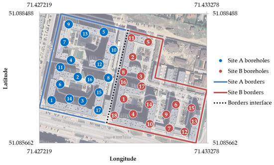
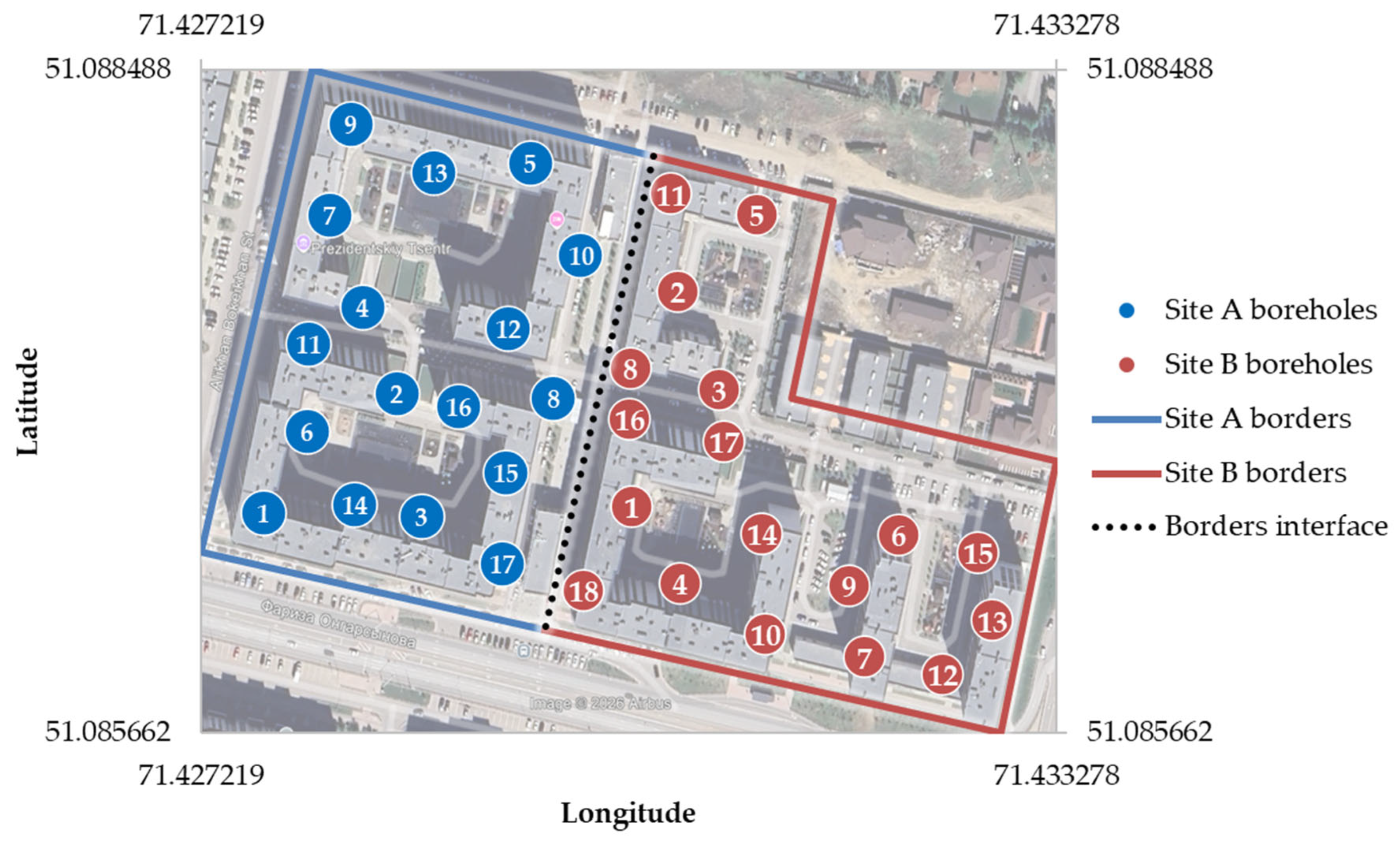
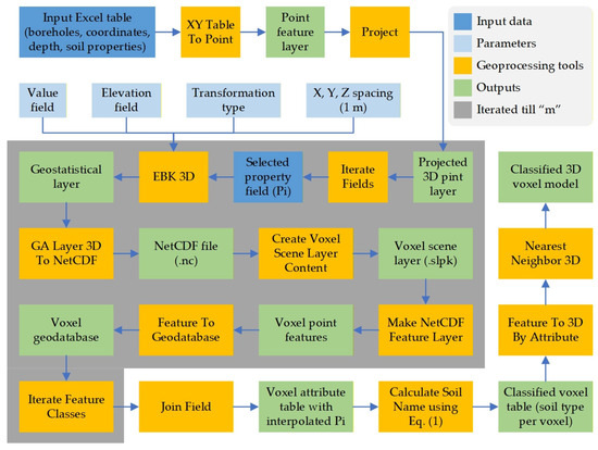
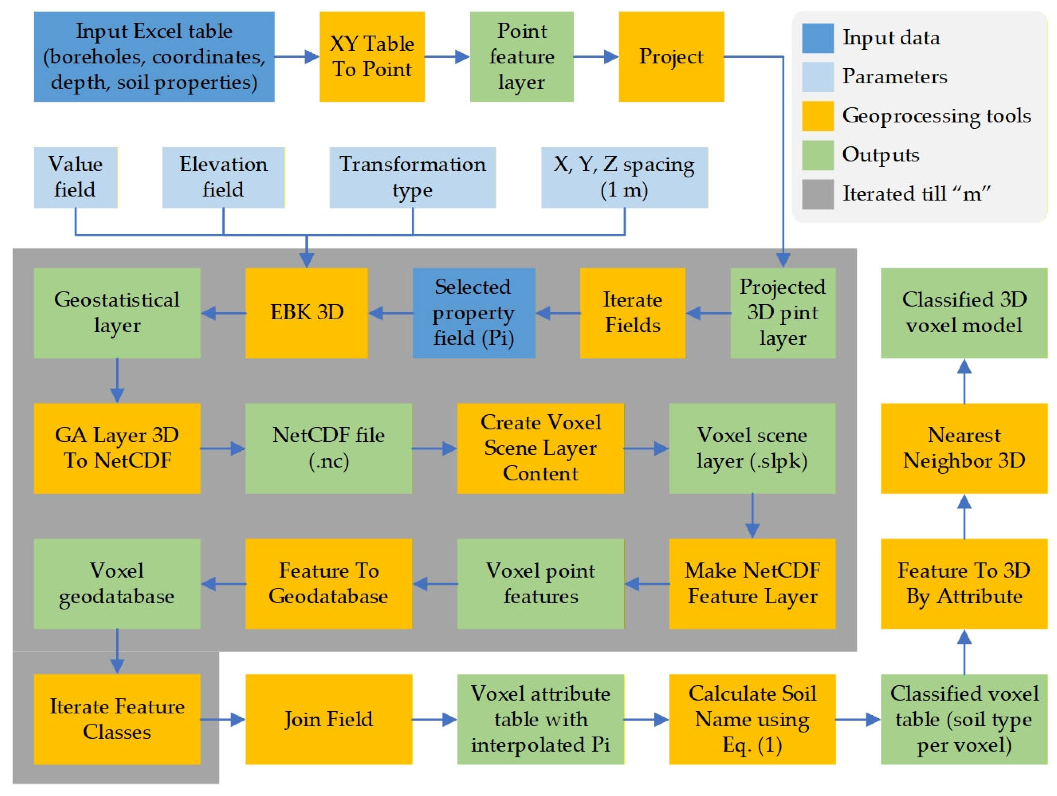
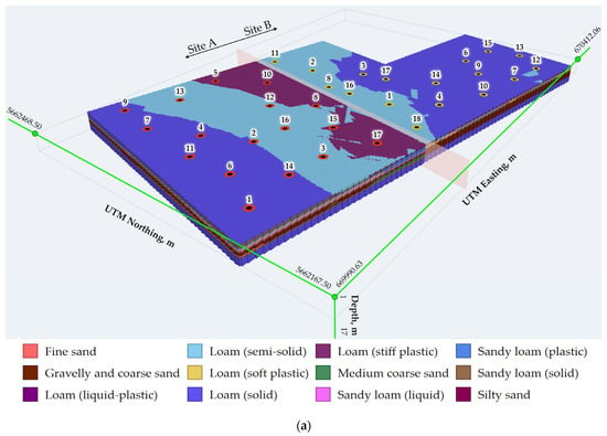
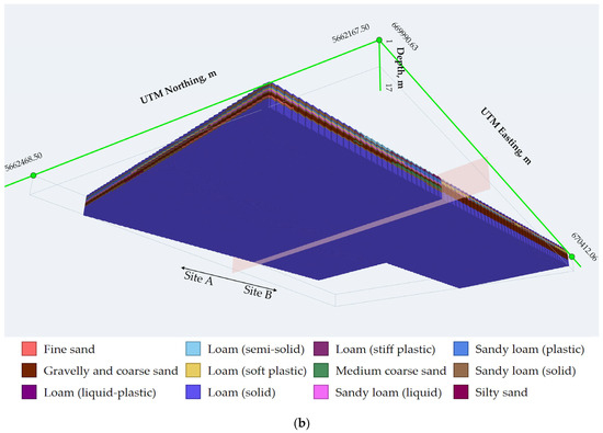
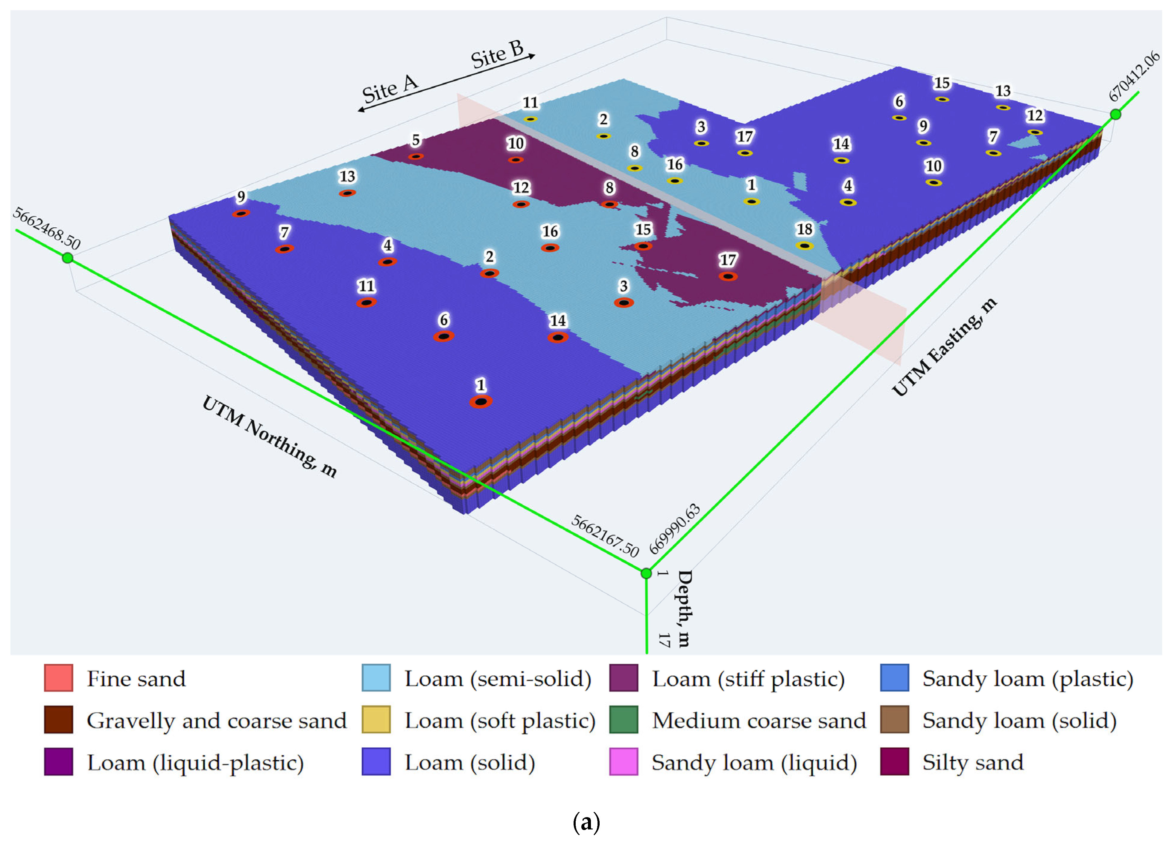
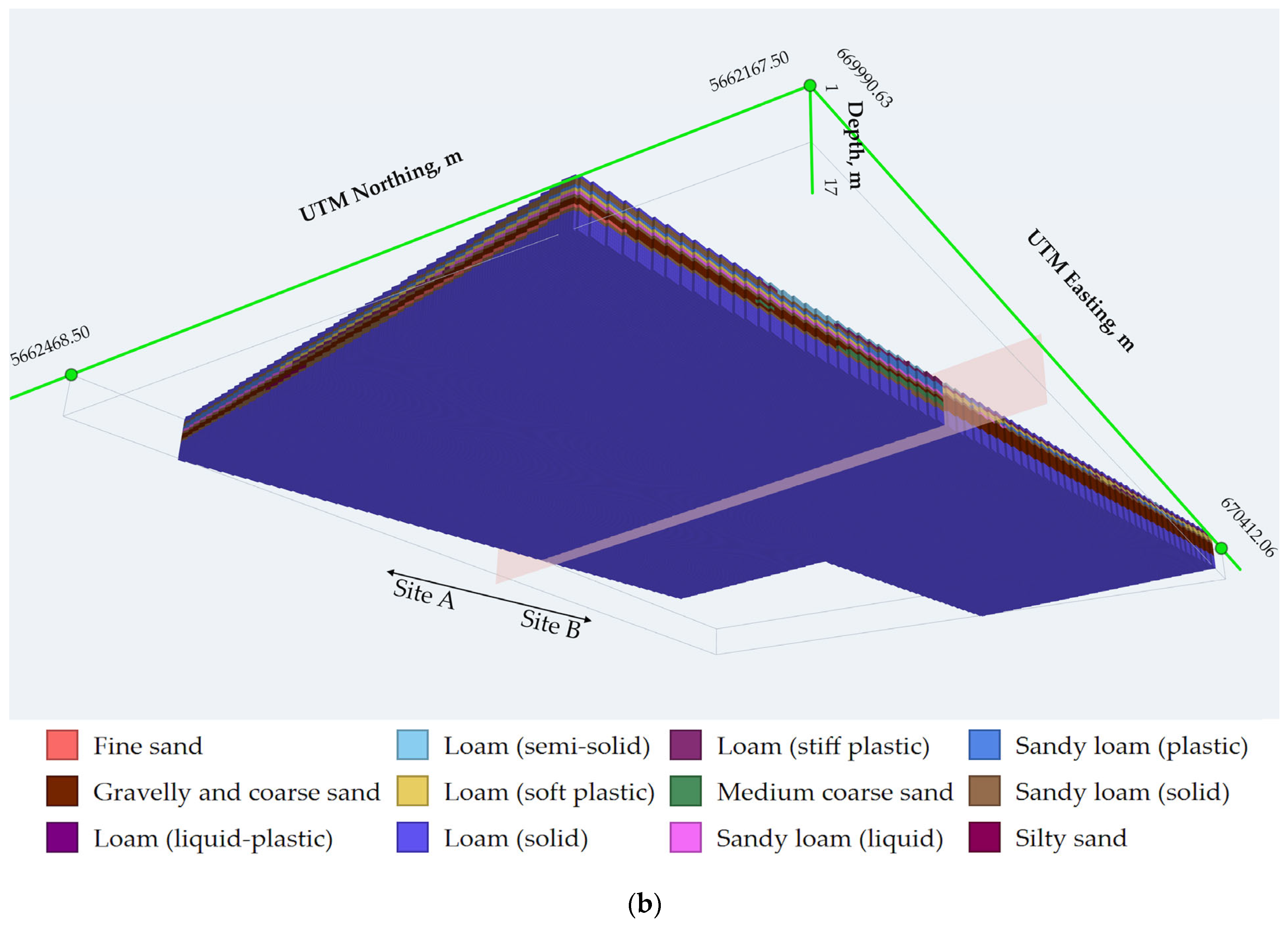
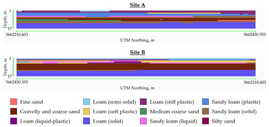
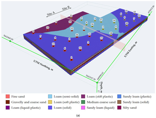
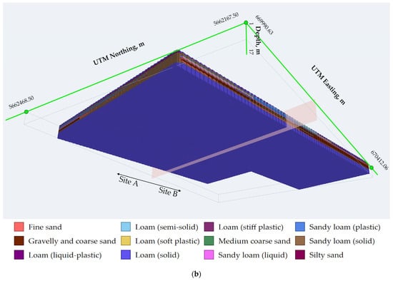
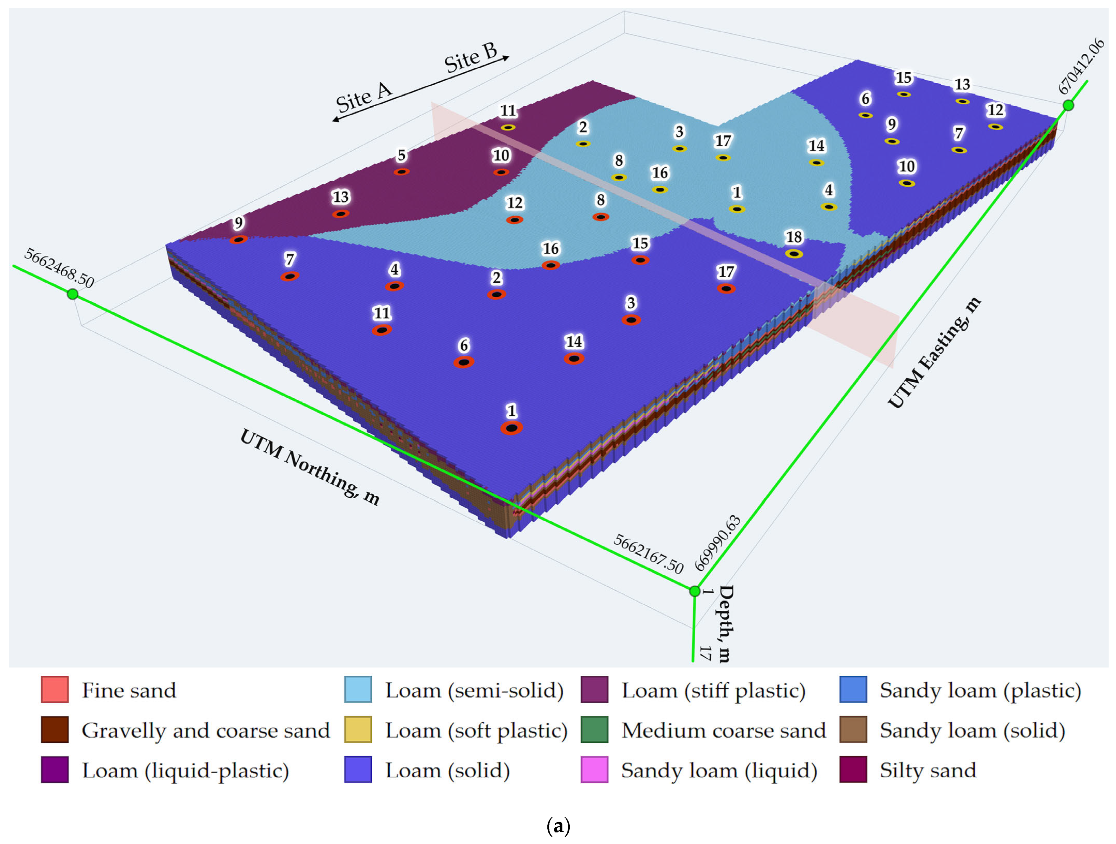
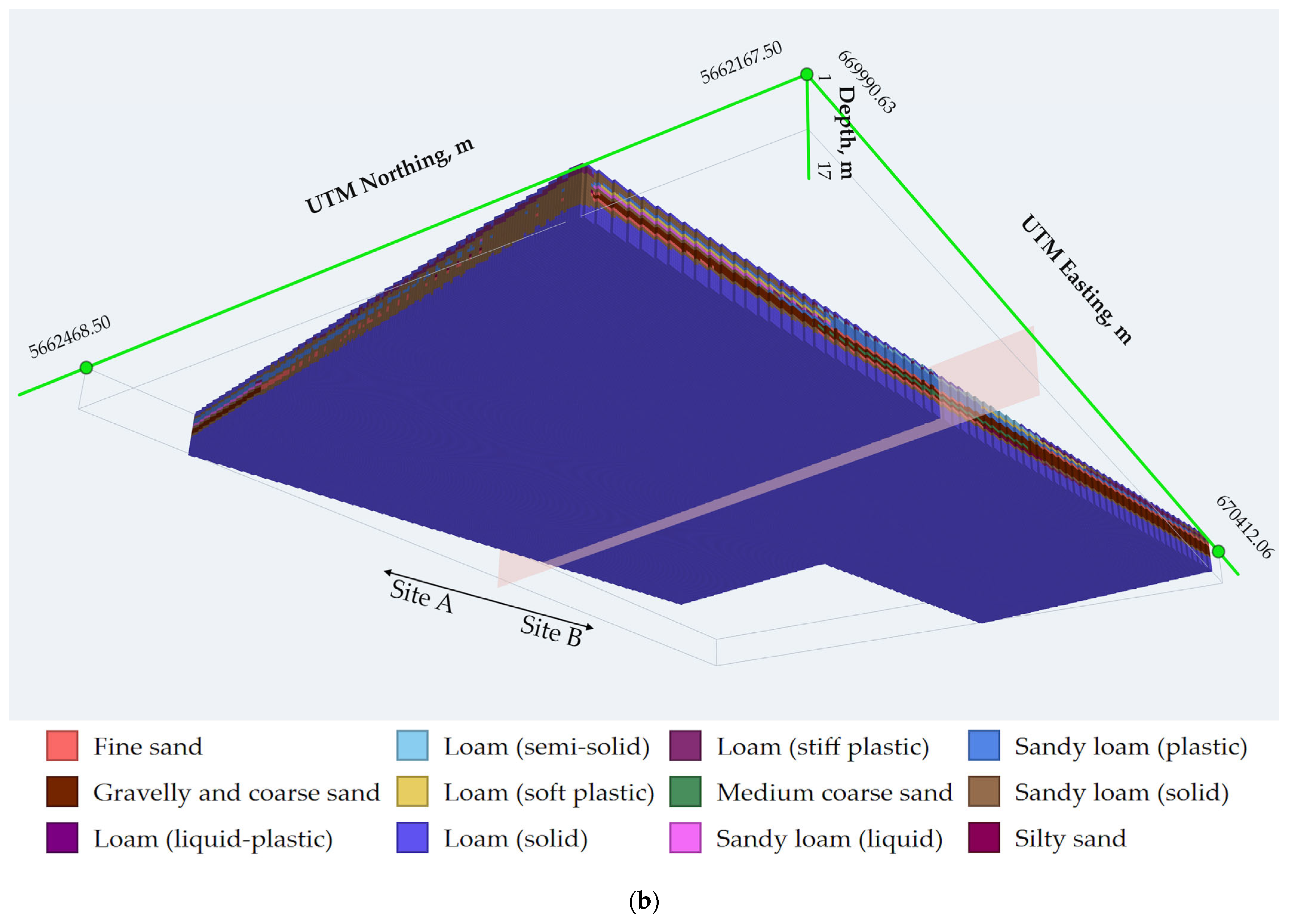
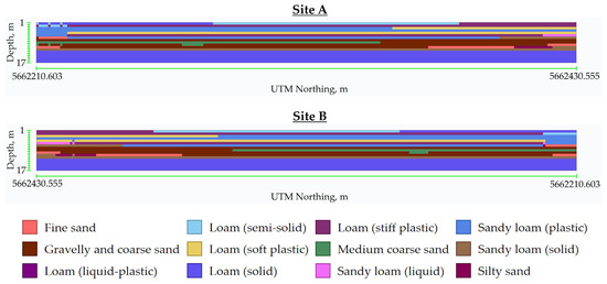
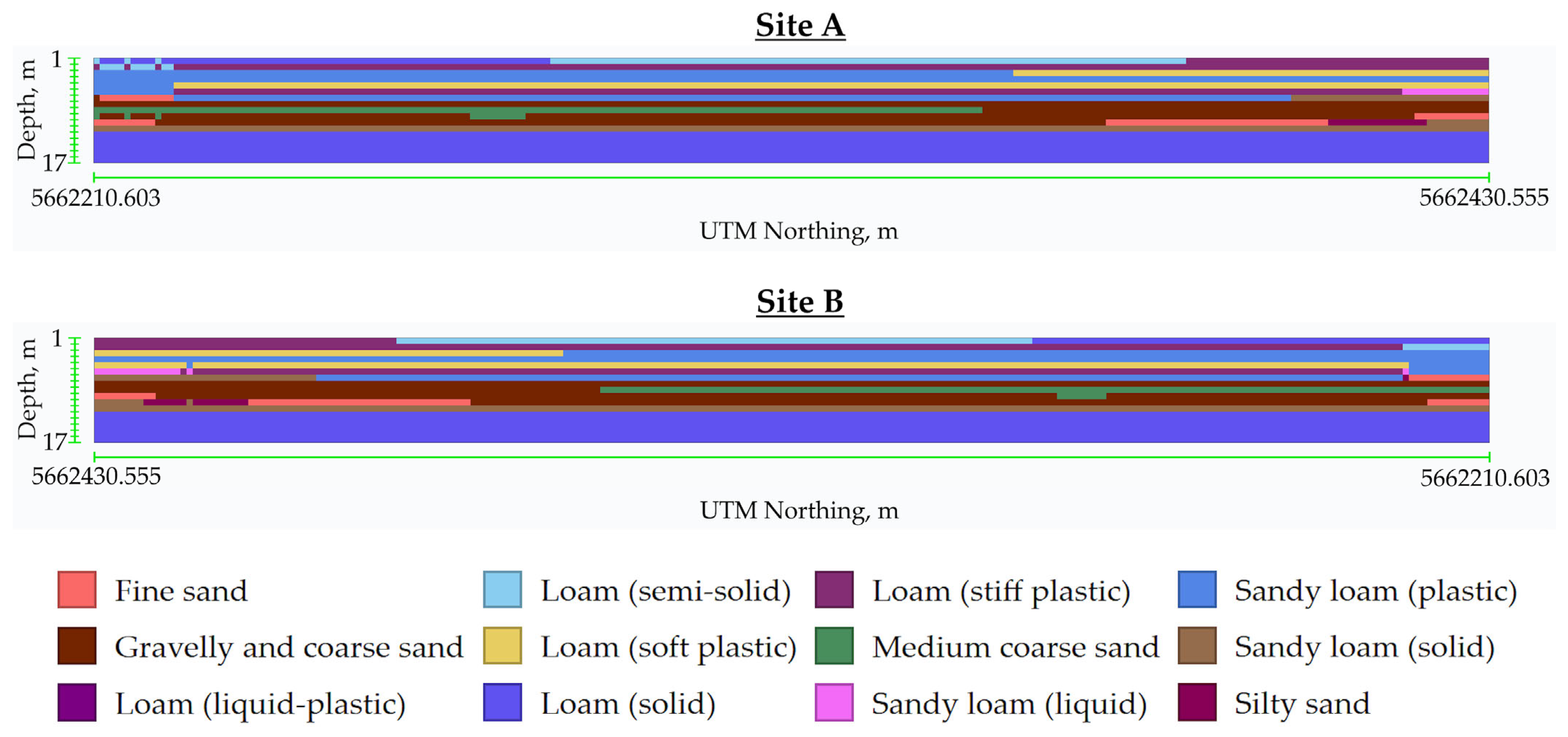
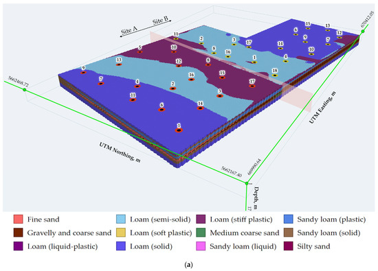
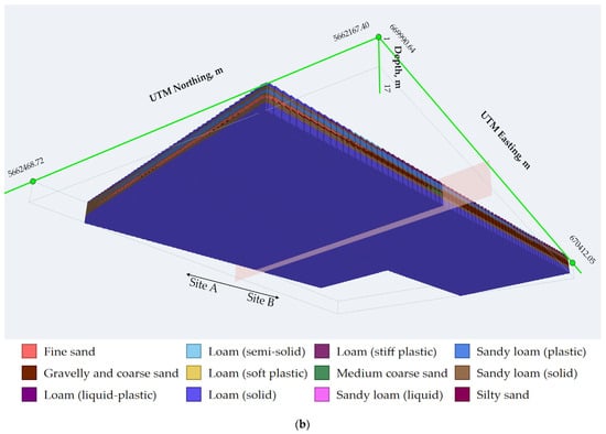
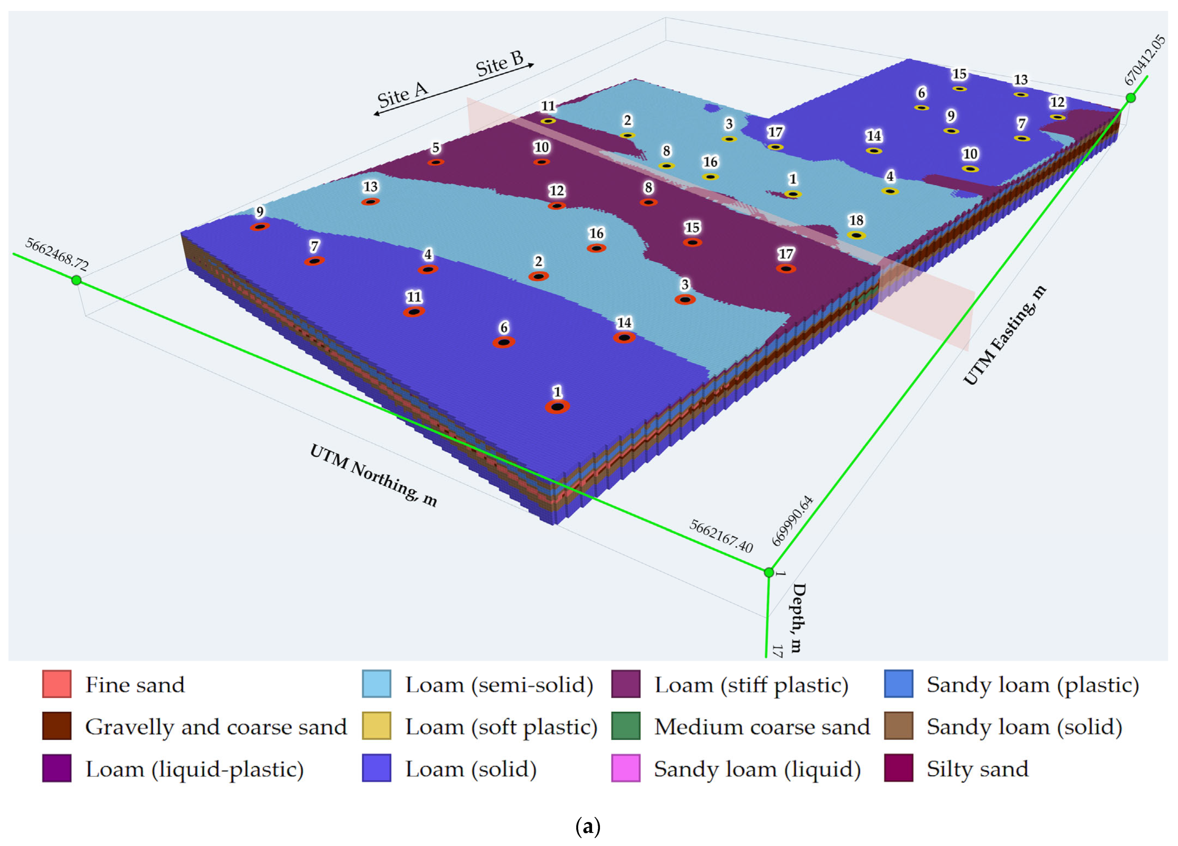
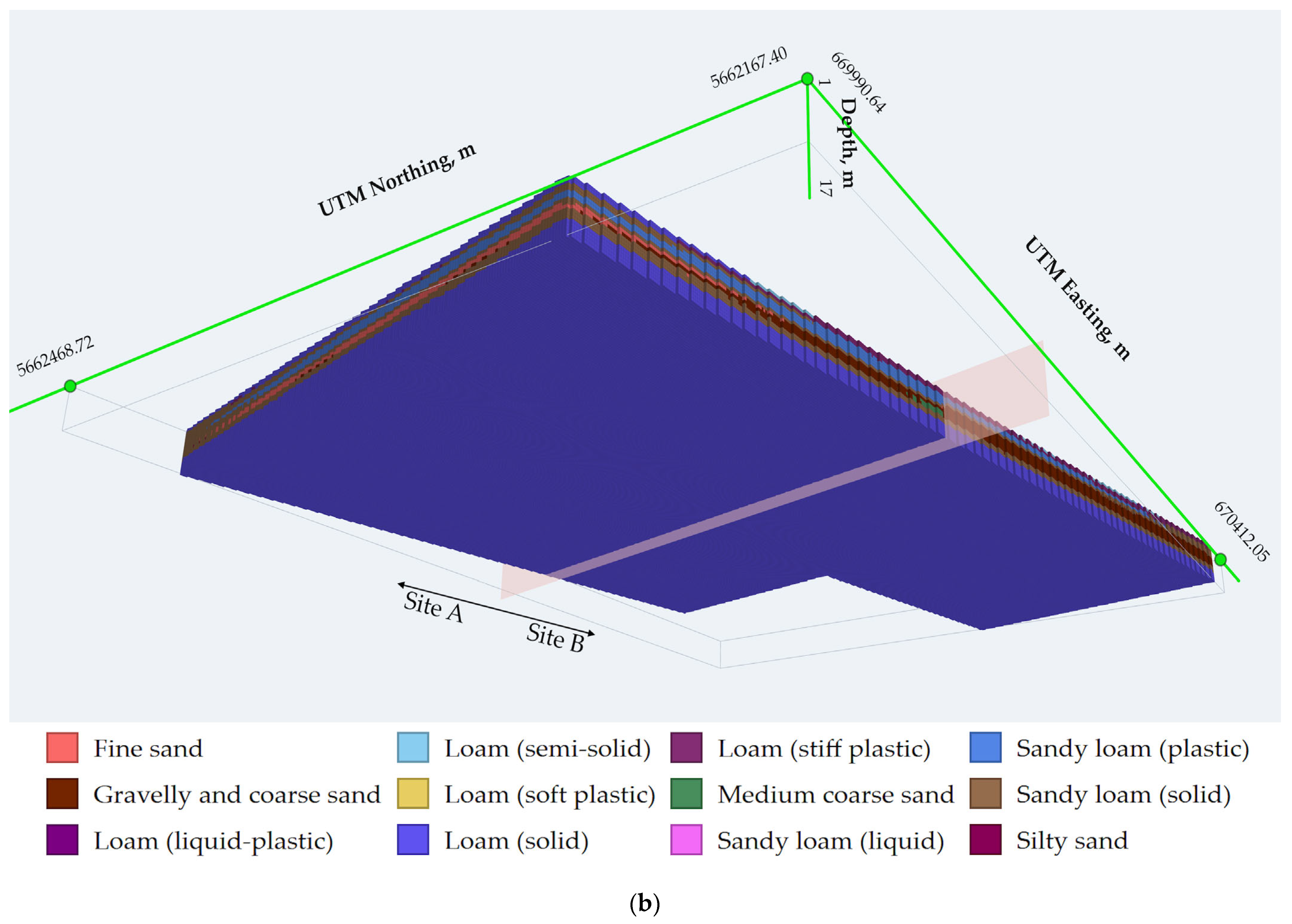
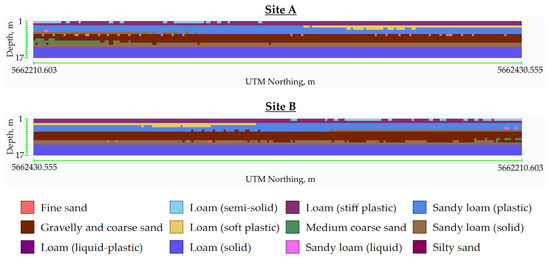

Disclaimer/Publisher’s Note: The statements, opinions and data contained in all publications are solely those of the individual author(s) and contributor(s) and not of MDPI and/or the editor(s). MDPI and/or the editor(s) disclaim responsibility for any injury to people or property resulting from any ideas, methods, instructions or products referred to in the content. |
© 2026 by the authors. Licensee MDPI, Basel, Switzerland. This article is an open access article distributed under the terms and conditions of the Creative Commons Attribution (CC BY) license.