Construction Material Classification from Terrestrial Laser Scanning Using a Reflectance-Related Radiometric Descriptor, Multiscale Geometric Roughness Features, and Automated Machine Learning

Abstract

Construction material identification is important for automated construction monitoring, digital twin generation, and building information modelling. Terrestrial laser scanning (TLS) provides dense geometric information together with LiDAR intensity measurements; however, reliable material discrimination remains challenging because intensity is affected by acquisition geometry and surface texture may vary depending on the spatial scale at which it is characterised. This study proposes a TLS-only machine-learning framework combining a reflectance-related intensity–geometry regression descriptor with multiscale geometric roughness features. Plane-residual roughness and normal-variation roughness were calculated using local cube neighbourhoods with side lengths of 0.10, 0.20, and 0.30 m. To avoid ambiguity associated with surface-normal orientation, the normal-variation descriptor was calculated using orientation-invariant angular differences between neighbouring surface normals. The training dataset was balanced using distance-stratified random undersampling, while the held-out test dataset retained its original class distribution. FLAML was used for automated model selection and hyperparameter optimisation using three-fold cross-validation with macro F1-score as the optimisation metric. The final stacking classifier achieved an overall accuracy of 90.44%, balanced accuracy of 87.42%, and macro F1-score of 87.85% on 1,296,822 held-out test points. The held-out test data were acquired from different scanner positions and spatially distinct material regions from those used for training, with no shared point samples; however, both datasets originated from the same general study area, and broader cross-site generalisation therefore requires further independent validation. Most material classes showed strong discrimination, although Carpet remained challenging because of confusion with Asphalt. The results demonstrate the potential of combining TLS-derived radiometric information with multiscale geometric surface descriptors for construction material classification without relying on RGB colour information.

1. Introduction

Construction material identification plays a critical role in automated construction monitoring, digital twin generation, and building information modelling (BIM) [1]. Terrestrial laser scanning (TLS) has emerged as a powerful technology for capturing high-resolution three-dimensional representations of construction environments, providing both geometric information and radiometric measurements in the form of LiDAR intensity [2,3].

Despite its potential, reliable material classification using TLS data remains challenging. Raw LiDAR intensity is influenced by geometric factors such as scanning distance and incidence angle, making it difficult to directly interpret as a material property [2,3,4]. Although previous studies have shown that radiometric correction can improve the stability of intensity-based features, materials with similar reflectance characteristics often remain difficult to distinguish. To address this limitation, geometric descriptors such as surface roughness have been introduced; however, most existing approaches rely on a limited representation of surface texture.

Furthermore, many approaches incorporate image-based colour features to improve classification performance. While effective under controlled conditions, these features are highly dependent on illumination and environmental conditions, reducing their reliability in practical construction scenarios [5].

To address these challenges, this study proposes a machine-learning framework that integrates radiometric and multiscale geometric descriptors derived solely from TLS point clouds. A reflectance-related radiometric descriptor is derived from the local relationship between measured LiDAR intensity and a geometry-dependent factor, while plane-residual roughness and normal-variation roughness are calculated at multiple neighbourhood scales to capture both surface-height variation and directional geometric structure. These TLS-derived features are then used within an automated machine-learning framework to identify an effective classification model.

The central hypothesis of this study is that combining a reflectance-related radiometric descriptor with multiscale geometric roughness information can improve the discrimination of construction materials compared to using a single roughness scale, while avoiding reliance on RGB colour information.

The main contributions of this study are:

• The integration of a reflectance-related radiometric descriptor with multiscale plane-residual and normal-variation roughness features for material representation;
• The use of normal-variation roughness to capture directional surface variation complementary to conventional plane-residual roughness;
• The application of an AutoML framework to select and combine suitable classifiers for the resulting TLS-derived feature set.

The proposed approach therefore aims to provide a discriminative TLS-derived feature representation that does not rely on RGB colour information and is consequently less dependent on ambient illumination and image-acquisition conditions.

2. Related Work

This section reviews the key concepts and prior studies relevant to material classification using terrestrial laser scanning (TLS). First, the radiometric properties of TLS data, including intensity and reflectance estimation, are discussed, with emphasis on the influence of geometric factors such as range and incidence angle. Next, existing radiometric correction methods are reviewed to highlight approaches for obtaining stable reflectance-related features. Finally, studies on construction material classification using TLS attributes are examined, focusing on the role of geometric descriptors such as surface roughness. This review establishes the foundation for the proposed approach, which integrates a reflectance-related radiometric descriptor with multiscale plane-residual and normal-variation roughness features within an automated machine-learning framework.

2.1. TLS Intensity as a Radiometric Cue for Material Characterisation

Terrestrial laser scanners record point coordinates and an associated intensity (backscatter) value, which provides additional information beyond geometry and can support semantic interpretation of surfaces [4]. However, raw TLS intensity is not a direct measure of intrinsic reflectance because it is affected by acquisition configuration and system-dependent factors [3]. The literature shows that intensity varies systematically with range and incidence angle, and that these effects differ across instruments and target types [2]. As a result, intensity-driven classification without correction can exhibit poor repeatability across scan stations and geometries [2,3].

Early correction research established two broad strategies: model-driven approaches based on the LiDAR/radiometric equation and surface reflection models, and data-driven approaches that fit empirical correction functions using calibration targets or overlap constraints [3,4]. These studies demonstrate that radiometric processing is a prerequisite when intensity is used as a material descriptor rather than a qualitative image [3,4].

2.2. Radiometric Correction and Remaining Challenges

Radiometric correction aims to reduce the influence of acquisition geometry on TLS intensity so that the resulting descriptor better represents material reflectance. Previous studies have shown that scanning distance and incidence angle are primary sources of intensity variation, although the exact response can differ between instruments, target materials, and surface conditions [2,6,7]. Kukko et al. [7] specifically quantified the influence of incidence angle on laser scanner intensity and surface data, while Kaasalainen et al. [2] investigated both distance and incidence-angle effects and proposed practical correction strategies. Correction approaches generally include model-driven methods based on the LiDAR/radiometric equation and empirical methods based on calibration targets, overlap constraints, or fitted correction functions [3,4,8]. More advanced approaches have also incorporated non-Lambertian reflection behaviour, such as Phong- and Oren–Nayar-based models, to account for specular effects and rough-surface scattering [9,10,11].

Reflectance retrieval methods further show that corrected intensity can approximate intrinsic surface reflectance more closely than raw intensity when distance and incidence-angle effects are compensated [12,13]. Despite these developments, corrected intensity or reflectance-like descriptors may still vary due to scanner-specific intensity definitions, internal gain/control, instrument drift, surface moisture, material finish, and local surface structure [3,14]. Recent studies have continued to refine radiometric correction by examining the theoretical independence of distance and incidence-angle effects and by applying intensity correction to improve mapping performance in practical LiDAR applications [15,16]. For TLS specifically, automated in situ radiometric calibration has also been proposed to compensate for distance and incidence-angle effects using overlapping scans [17].

Therefore, reflectance or reflectance-related radiometric descriptors alone may be insufficient for distinguishing construction materials with overlapping radiometric responses. This motivates the use of complementary geometric information and, in particular, the investigation of roughness descriptors at multiple spatial scales together with radiometric TLS features.

2.3. Roughness Descriptors as Complementary Geometric Features

Surface roughness is commonly derived from local point-cloud neighbourhoods using plane fitting, residual analysis, or related geometric statistics that describe micro-scale surface variation independently of global surface orientation [18]. Because roughness is computed directly from 3D geometry, it provides information that is complementary to radiometric descriptors and can improve class separability when different materials have similar reflectance responses [18,19]. Descriptor choice and neighbourhood scale are important because different roughness formulations can produce different roughness maps and influence material discrimination [18]. A single fixed neighbourhood may emphasise only one level of surface structure, whereas construction materials can exhibit geometric texture over multiple spatial scales. Accordingly, evaluating roughness at multiple neighbourhood sizes can provide complementary information by capturing both finer and broader surface variations.

Roughness is also physically relevant to radiometric behaviour because local micro-geometry affects laser scattering and the observed intensity–angle relationship [9,11,17]. This relationship is supported by recent work using polarimetric multispectral LiDAR, which showed that material type and surface roughness can be co-discriminated when radiometric measurements capture scattering-related differences [20]. Therefore, combining a reflectance-related radiometric descriptor with explicit geometric roughness descriptors can provide a more complete representation of construction material properties than using radiometric information alone.

2.4. Construction-Oriented Material Discrimination Using TLS Attributes

Construction material classification using TLS attributes has been investigated as an alternative to image-based material recognition because TLS provides co-located geometric and radiometric information [19]. Yuan et al. [19] demonstrated that common building materials can be classified using reflectance, HSV colour, and surface roughness, and showed that multi-attribute fusion improves classification accuracy compared with single-feature approaches. However, their highest performance relied on HSV colour features, which remain dependent on image-acquisition and illumination conditions. Their LiDAR-only feature set, based on reflectance and plane-residual roughness, achieved lower classification accuracy. However, performance values reported by Yuan et al. [19] should not be interpreted as a direct benchmark for the present study because the studies differ in material composition, scanner configuration, sampling strategy, and evaluation protocol. Their work is therefore used primarily as a methodological reference for TLS-based material discrimination.

These findings indicate that TLS-derived radiometric and geometric features are promising, but that additional LiDAR-only geometric information is required to reduce reliance on RGB/HSV features. In particular, conventional point-to-plane roughness calculated at a single neighbourhood scale may not fully represent either directional surface variation or the scale-dependent nature of material texture. The present study addresses this gap by combining a reflectance-related radiometric descriptor with both plane-residual roughness and normal-variation roughness calculated at multiple spatial scales within an AutoML-based classification framework.

2.5. Learning Models for Fused Radiometric–Geometric Material Classification

AutoML frameworks can support model development by automating algorithm selection and hyperparameter tuning under computational constraints. FLAML is a lightweight AutoML framework designed to identify accurate models with low computational cost [21]. This is relevant for TLS-derived material classification because performance depends not only on the selected classifier, but also on stable feature design, preprocessing choices, acquisition quality, and model generalisation.

When radiometric and geometric descriptors are represented as engineered features, material classification can be formulated as a structured tabular learning problem. Different machine-learning algorithms may respond differently to nonlinear relationships and interactions among these descriptors. Rather than preselecting a single classifier, the present study therefore uses FLAML to evaluate multiple candidate algorithms and hyperparameter configurations under a common optimisation framework. Recent reviews of point-cloud learning also emphasise that data quality, acquisition heterogeneity, preprocessing, and domain shift remain important considerations for classification performance [1,22,23,24]. The final predictive model is consequently determined empirically from the training data rather than being fixed in advance.

3. Methodology

3.1. Data Acquisition Using Terrestrial Laser Scanning

Point-cloud data used in this study were collected using a Trimble TX8 terrestrial laser scanner, a time-of-flight LiDAR system operating at a wavelength of approximately 1.5 µm in the near-infrared region, which is invisible to the human eye. The scanner captures high-density three-dimensional point clouds together with backscattered laser intensity measurements.

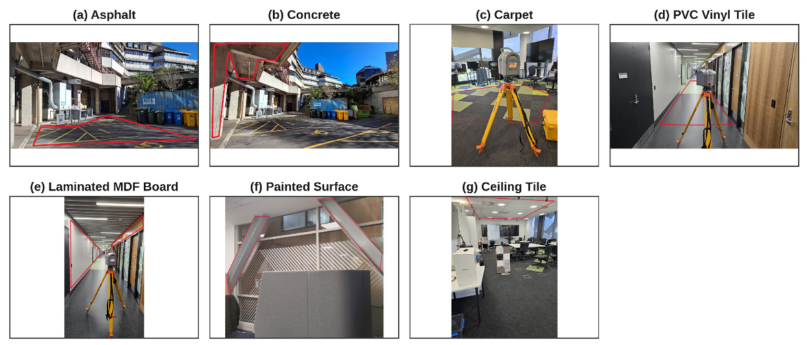
A set of commonly encountered construction materials was selected for the experiments, including Asphalt, Concrete, Carpet, PVC Vinyl Tile, Laminated MDF Board, Painted Surface, and Ceiling Tile as shown in Figure 1.

Asphalt and Concrete surfaces were captured under outdoor conditions, while the remaining materials were acquired from indoor building surfaces. Rather than using isolated laboratory specimens, the dataset was obtained from real construction and building surfaces within the University of Auckland environment. This allowed the TLS measurements to include naturally occurring variation in surface condition, range, and acquisition geometry.

Only points located at scanning distances from 4 m up to, but not including, 10 m were retained for the analysis. Points outside this interval were excluded to maintain a consistent acquisition-distance range across all material classes.

The dataset was organised into separate training and held-out testing subsets acquired from different scanner positions and spatially distinct regions of the material surfaces. No point samples were shared between the training and test datasets. Although both subsets were collected within the same general study area, the use of different scan positions and non-overlapping material regions reduced the risk of point-level spatial leakage between model development and evaluation. After application of the distance criterion and validity checks for the final multiscale feature set, the unbalanced training dataset contained 1,141,122 points, while the held-out test dataset contained 1,296,822 points. Class balancing was applied only to the training dataset, as described in Section 3.4.3, while the primary test dataset retained its original class distribution.

3.2. Reflectance-Related Radiometric Descriptor from LiDAR Intensity

As discussed in Section 2, TLS intensity is influenced by acquisition geometry and cannot be directly interpreted as an intrinsic material property. Therefore, in this study, a geometric correction was applied to derive a reflectance-related descriptor. The radiometric behaviour of LiDAR backscatter can be approximated using a simplified laser radar model:

$$I_r={\displaystyle \frac{K\rho \mathit{cos}\left(\theta \right)}{R^2}}+b,$$

(1)

where

• $I_r$ is the recorded LiDAR intensity;
• $\rho$ represents the intrinsic reflectance of the surface;
• $R$ is the distance between the scanner and the target point;
• $\theta$ is the incidence angle between the laser beam and the surface normal;
• $K$ is a system constant related to sensor characteristics;
• $b$ represents a bias term associated with sensor noise.

Equation (1) provides the physical motivation for accounting for range and angular effects in the measured TLS intensity. In the implemented workflow, however, an absolute surface reflectance coefficient was not calculated. Instead, a relative reflectance-related radiometric descriptor was derived from the local relationship between measured intensity and a geometry-dependent factor, following the general formulation used by Yuan et al. [19].

For each point, the scanning distance was calculated from its three-dimensional co- ordinates relative to the scanner. A coordinate-derived angular factor was also calculated from the point position. Following the formulation adopted from Yuan et al. [19], this angular term is denoted by (cos θ) and is used as a geometric approximation rather than as a directly measured incidence angle based on an independently estimated surface normal. The resulting distance-and-angle-dependent quantity was used as the explanatory variable for local intensity regression.

A Euclidean neighbourhood with a radius of 0.10 m was defined around each point. Neighbourhoods containing fewer than 20 points were excluded from this calculation. Within each valid neighbourhood, an ordinary least-squares linear regression with an intercept was fitted between the measured LiDAR intensity and the geometry-dependent explanatory variable. The fitted regression slope, denoted here as Slope_SKL, was retained as the reflectance-related radiometric descriptor used for classification.

Slope_SKL should therefore be interpreted as a relative local intensity–geometry regression descriptor rather than an absolute physical reflectance coefficient. Because the slope is estimated locally from measured intensity values, it is not constrained to be positive. Negative values can occur where local intensity variations, measurement noise, surface heterogeneity, or a weak local intensity–geometry relationship produce a negative fitted gradient. These values were retained rather than truncated because they form part of the empirically derived feature distribution.

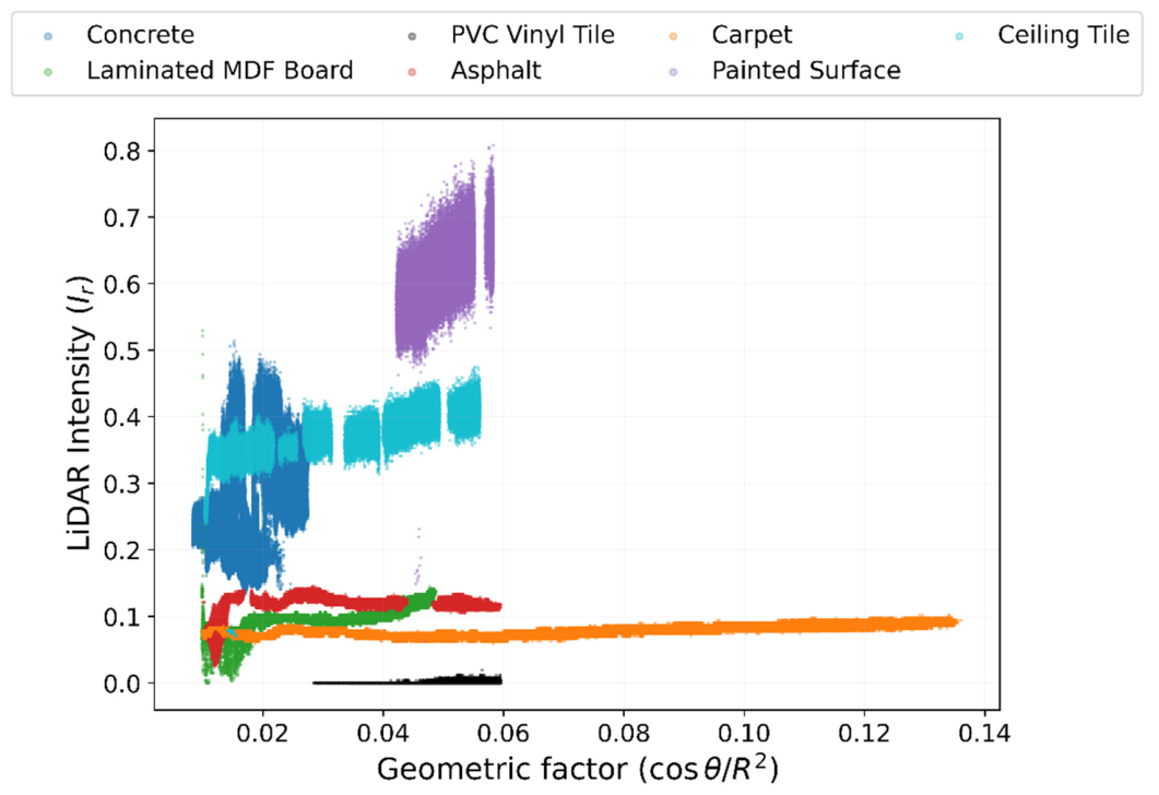
Figure 2 illustrates the relationship between measured LiDAR intensity and the geometry-dependent factor for representative construction materials. Differences in the local intensity–geometry response between materials provide the basis for using the fitted regression slope as a radiometric classification feature.

The resulting Slope_SKL descriptor was used directly as one of the machine-learning predictors. No calibration targets with known reflectance values were required, and the descriptor was not interpreted as an absolute or intrinsic reflectance measurement.

3.3. Surface Roughness Estimation from Point Clouds

Surface roughness describes the micro-scale geometric variability of a material sur- face and provides important information for distinguishing materials with similar radio- metric responses. In terrestrial laser scanning (TLS), roughness can be derived directly from the local geometry of the point cloud by analysing the spatial distribution of neighbouring points. Unlike reflectance, which represents radiometric properties, roughness captures the structural characteristics of surface texture.

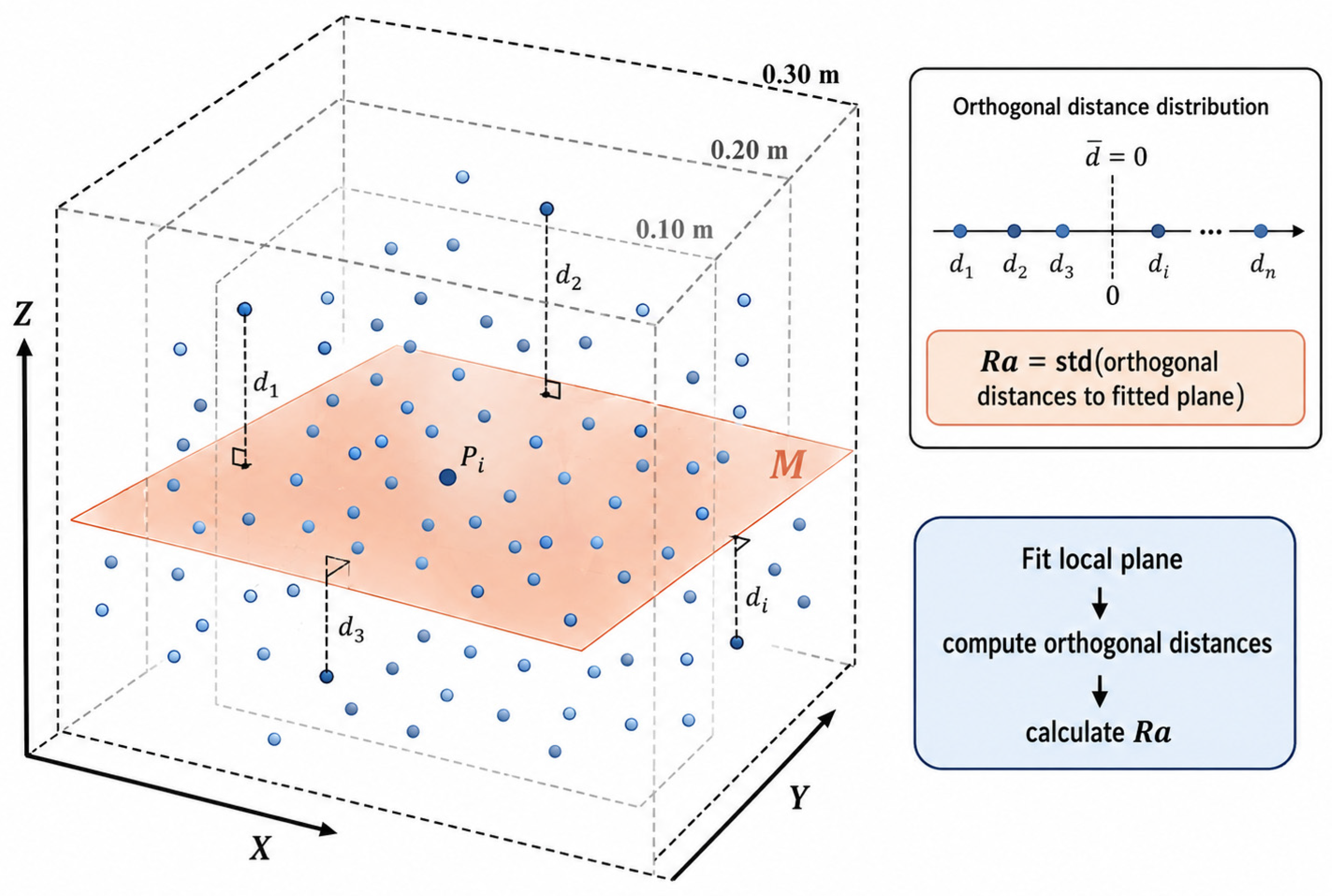
For each point, local neighbourhoods were defined as cubes with side lengths of 0.10, 0.20, and 0.30 m, centred on the point and identified using a KD-tree with a Chebyshev-distance metric. These neighbourhood sizes were used to capture surface variation at different spatial scales. The 0.20 m scale maintains comparability with the roughness calculation used by Yuan et al. [19], while the 0.10 and 0.30 m scales provide finer- and broader-scale representations of local surface structure. Neighbourhoods containing fewer than 20 points were excluded from the corresponding roughness calculation to avoid unstable plane and normal estimates in sparsely sampled regions. Within each valid neighbourhood, a local plane was fitted using the Random Sample Consensus (RANSAC) algorithm according to the general plane equation:

$$Ax+By+Cz+D=0,$$

(2)

Candidate planes were generated from randomly sampled point triplets, with a maximum of 100 trials. Neighbouring points with an orthogonal distance of less than 2 mm from a candidate plane were treated as inliers. After identification of the largest inlier set, the plane was refitted using singular value decomposition (SVD) to obtain a least-squares estimate of the final plane parameters. This formulation is independent of surface orientation and is therefore applicable to horizontal, inclined, and vertical surfaces.

Figure 3 illustrates the calculation of plane-residual roughness using a local point-cloud neighbourhood, a fitted plane, and the orthogonal distances of neighbouring points from the plane.

$$R_a=\surd [(1/n) {{\Sigma }_{\mathrm{i}=1}}^{\mathrm{n}} {(d_{\mathrm{i}}-\mu )}^2],with \mu =(1/n) {{\Sigma }_{\mathrm{i}=1}}^{\mathrm{n}}{d}_{\mathrm{i}} ,$$

(3)

where $d_i$ represents the unsigned orthogonal distance between neighbouring point $i$ and the locally fitted plane, and $n$ denotes the number of points in the neighbourhood. Ra was calculated as the population standard deviation of these orthogonal distances. The same procedure was applied separately at the 0.10, 0.20, and 0.30 m neighbourhood scales, producing three plane-residual roughness descriptors for each valid point.

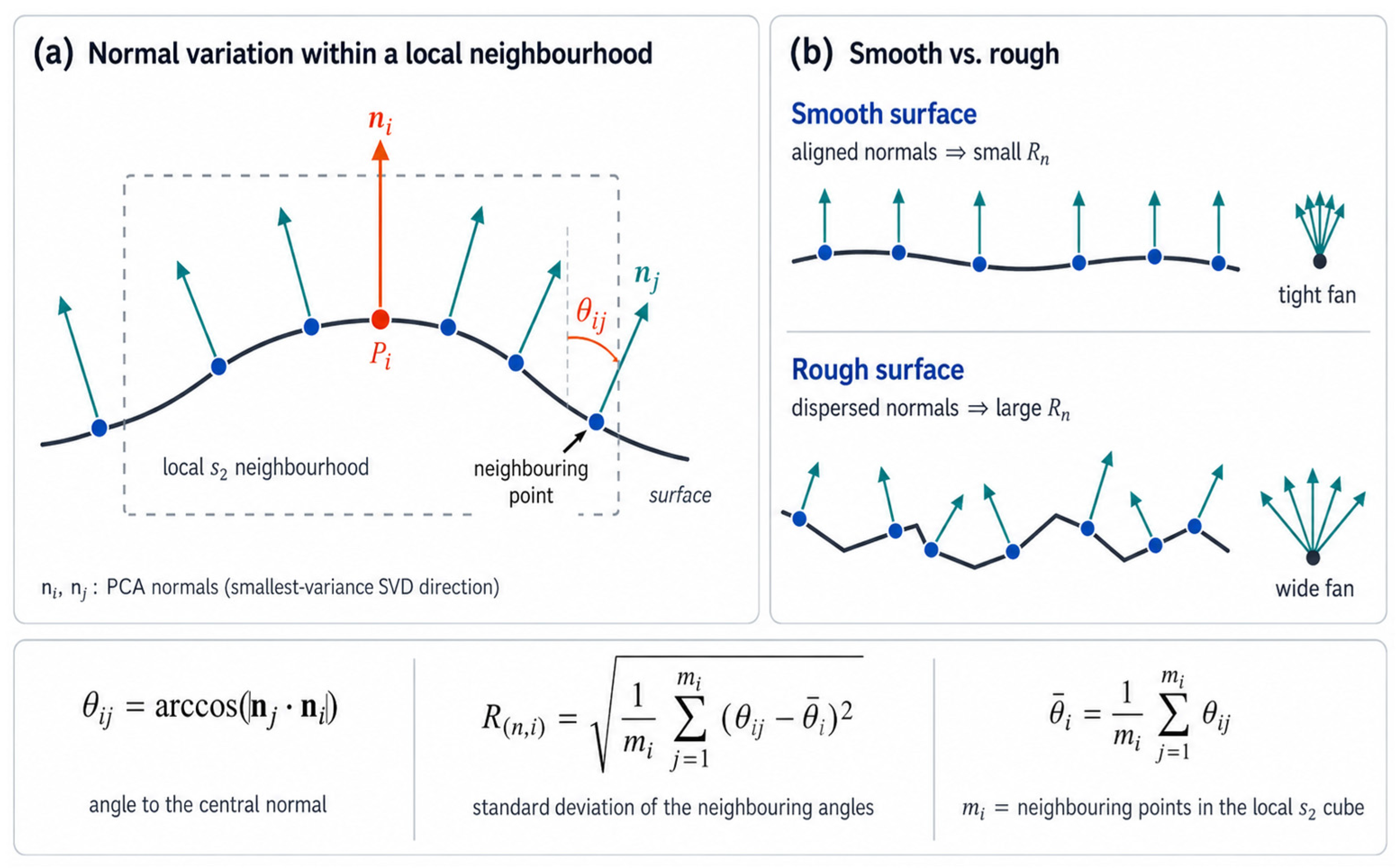
Although Ra captures the magnitude of point-to-plane surface variation, it does not fully represent directional changes in local surface geometry. A second descriptor, nor- mal-variation roughness ($Rn$), was therefore calculated from the angular variation in neighbouring surface normals. For each central point, a unit normal vector was estimated using PCA/SVD within the corresponding local neighbourhood. Because PCA/SVD-de- rived normal vectors have an arbitrary sign, the angular difference between the central- point normal and each valid neighbouring-point normal was calculated using the absolute value of their dot product. This makes the angular difference invariant to normal-vector orientation. $Rn$ was then defined as the population standard deviation of these angular deviations and was expressed in radians:

$${\theta }_{ij}={\cos }^{-1}\left(|{\mathbf{n}}_i\cdot {\mathbf{n}}_j|\right), {\overline{ \theta }}_i={\displaystyle \frac{1}{m_i}}{\displaystyle {\sum }_{j=1}^{m_i}}{\theta }_{ij},{ R}_{n,i}=\sqrt{{\displaystyle \frac{1}{m_i}}{\displaystyle {\sum }_{j=1}^{m_i}}{\left({\theta }_{ij}-{\overline{\theta }}_i\right)}^2},$$

(4)

As illustrated in Figure 4, the normal-variation roughness descriptor quantifies the angular dispersion between the surface normal of each neighbouring point and the surface normal estimated at the central point within a local neighbourhood.

Where n_i is the unit normal vector estimated at the central point P_i, n_j is the unit normal vector estimated at neighbouring point P_j, θ_ij is the angular deviation between the two normal vectors, ${\overline{\theta }}_i$ is the mean angular deviation within the valid neighbourhood, and m_i is the number of valid neighbouring points with estimated normal vectors. The resulting Rn,_i value is expressed in radians and represents the local angular dispersion of surface normals [25,26].

Together, the multiscale $R_a$ and $Rn$ descriptors characterise two complementary aspects of local surface geometry: the magnitude of point-to-plane deviations and the directional variation in surface normals. Calculating both descriptors at multiple neighbourhood scales enables finer and broader surface structures to be represented within the classification feature set [27].

3.4. Machine-Learning Framework for Material Classification

3.4.1. Feature Construction

The final classification feature set was designed to combine radiometric information with geometric surface characteristics measured at multiple spatial scales. For each valid TLS point, seven predictors were used:

• Slope_SKL, representing the local reflectance-related intensity–geometry regression descriptor described in Section 3.2;
• $R_a$ at 0.10 m, representing plane-residual roughness calculated using a 0.10 m cube neighbourhood;
• $Rn$ at 0.10 m, representing normal-variation roughness calculated using a 0.10 m cube neighbourhood;
• $R_a$ at 0.20 m, representing plane-residual roughness calculated using a 0.20 m cube neighbourhood;
• $Rn$ at 0.20 m, representing normal-variation roughness calculated using a 0.20 m cube neighbourhood;
• $R_a$ at 0.30 m, representing plane-residual roughness calculated using a 0.30 m cube neighbourhood;
• $Rn$ at 0.30 m, representing normal-variation roughness calculated using a 0.30 m cube neighbourhood.

Together, these predictors combine one radiometric descriptor with six geometric descriptors representing plane-residual and normal-variation roughness at three spatial scales. This multiscale feature representation was used to capture both fine and broader variations in material surface structure.

The predictor set therefore consisted of Slope_SKL and the six multiscale Ra and Rn features. Point coordinates, raw LiDAR intensity, RGB colour values, scanning distance, material labels, and dataset identifiers were not included as predictor variables. The material class was used only as the classification target, while dataset identifiers were retained only for data organisation and evaluation.

3.4.2. Automated Machine Learning Using the Fast Lightweight Automated Machine Learning (FLAML)

The Fast Lightweight Automated Machine-Learning (FLAML) framework was used for automated model selection and hyperparameter optimisation [21]. FLAML performs cost-aware optimisation across multiple candidate machine-learning algorithms and their hyperparameter configurations within a specified computational budget. This approach was adopted to avoid manually preselecting a particular classifier and to allow the model configuration to be determined empirically from the training data.

In this study, the task was defined as multiclass classification using the seven TLS-derived predictors described in Section 3.4.1. Model optimisation was performed using three-fold cross-validation, with macro F1-score used as the optimisation metric so that performance across all seven material classes contributed equally to model selection.

A computational search budget of 900 s was specified for the AutoML optimisation. The candidate estimators evaluated during the FLAML search comprised LightGBM, XGBoost, limited-depth XGBoost, CatBoost, histogram-based gradient boosting, Random Forest, and Extra Trees. A fixed random seed of 42 was used to support reproducibility. Parallel computation was enabled during the search. FLAML’s automatic data augmentation and internal sampling options were disabled because class balancing had already been applied explicitly to the training dataset. Ensemble construction was enabled to allow FLAML to combine suitable trained models when this improved the optimisation objective.

The implementation used FLAML version 2.3.6, scikit-learn version 1.7.0, and Python version 3.13.2.

3.4.3. Model Training and Evaluation

The training and held-out test datasets were maintained separately throughout model development and evaluation. The two datasets were derived from different scanner positions and spatially distinct regions of the material surfaces, with no shared point samples between the training and held-out test sets. After feature validity checks, the unbalanced training dataset contained 1,141,122 points. The class-specific numbers of valid training and held-out test points are summarised in

Table 1. Number of valid points in the unbalanced training and held-out test datasets for each material class.

Material	Training Points	Test Points
Asphalt	274,748	254,336
Carpet	98,945	69,883
Ceiling Tile	126,294	97,700
Concrete	242,938	396,597
Laminated MDF Board	233,770	327,162
Painted Surface	100,131	92,131
PVC Vinyl Tile	64,296	59,013
Total	1,141,122	1,296,822

.

Because the number of observations differed substantially among material classes, class balancing was applied only to the training dataset before model optimisation.

The smallest training class contained 64,296 points. Therefore, each of the seven material classes was reduced to 64,296 observations using distance-stratified random undersampling without replacement, resulting in a balanced training dataset of 450,072 points. Sampling was performed within 0.25 m scanning-distance intervals to reduce distortion of the original distance distribution within each material class. A fixed random seed of 42 was used to make the sampling procedure reproducible.

The held-out test dataset was not balanced or resampled and retained its original class distribution, comprising 1,296,822 points. No test observations were used during class balancing, model selection, or hyperparameter optimisation. The seven predictors described in Section 3.4.1 were used as model inputs, while the material class served as the target variable.

Model selection and hyperparameter optimisation were performed on the balanced training dataset using the FLAML procedure described in Section 3.4.2. After model development was completed, the resulting fitted model was applied to the held-out test dataset without further training or parameter tuning.

Classification performance was evaluated using overall accuracy, balanced accuracy, macro-averaged precision, macro-averaged recall, macro F1-score, weighted precision, weighted recall, and weighted F1-score. A normalised confusion matrix and class-specific performance statistics were additionally examined to identify material classes and material pairs associated with the largest classification errors. The Python scripts reproducing the preprocessing, feature extraction, model training, held-out evaluation, and ablation workflow are provided in the Supplementary Materials.

3.5. Use of Generative Artificial Intelligence Tools

During the preparation of this manuscript, ChatGPT by (OpenAI, GPT-5.6 Sol) was used to assist with Python code development, figure, and language editing. The tool was not used to develop the study design, collect data, generate raw experimental data, conduct the analysis, extract features, train the model, or interpret the results. All methodological decisions, data processing, feature extraction, model training, result interpretation, and scientific conclusions were carried out by the authors. The authors reviewed and edited all AI-assisted outputs and take full responsibility for the accuracy, integrity, and content of the manuscript.

4. Results and Discussion

The final model obtained through the FLAML optimisation and ensemble-construction process was evaluated on the held-out test dataset containing 1,296,822 points. The test dataset retained its original class distribution and was not used during class balancing, model selection, or hyperparameter optimisation. The final stacking classifier achieved an overall classification accuracy of 90.44%, a balanced accuracy of 87.42%, and a macro F1-score of 87.85%. The weighted F1-score was 90.41%. The difference between overall accuracy and balanced accuracy reflects the unequal class distribution in the held-out test dataset and highlights the importance of reporting class-balanced metrics in addition to overall accuracy. The overall classification performance metrics are summarised in

Table 2. Classification performance of the final stacking classifier on the held-out test dataset.

Metric	Value
Accuracy	90.44%
Balanced Accuracy	87.42%
Precision (Macro Avg)	88.54%
Recall (Macro Avg)	87.42%
F1-score (Macro Avg)	87.85%
Precision (Weighted Avg)	90.70%
Recall (Weighted Avg)	90.44%
F1-score (Weighted Avg)	90.41%

.

To quantify the separate contributions of the radiometric and geometric descriptors, an ablation study was performed using four progressively enriched feature sets. All feature configurations were evaluated using the same balanced training dataset and the same held-out test dataset. The first scenario used only the reflectance-related radiometric descriptor, Slope_SKL. The second added the conventional single-scale plane-residual roughness calculated at 0.20 m. The third extended Ra to the three neighbourhood scales of 0.10, 0.20, and 0.30 m, while the fourth represented the complete proposed feature set by additionally including multiscale normal-variation roughness Rn. The results of the feature-ablation analysis are summarised in

Table 3. Ablation study showing the contribution of the reflectance-related radiometric descriptor, single-scale and multiscale plane-residual roughness, and multiscale normal-variation roughness to classification performance on the held-out test dataset.

Scenario	Feature Set	Accuracy	Balanced Accuracy	Macro F1	Weighted F1
S1	Slope_SKL only	48.17%	44.25%	37.25%	48.45%
S2	Slope_SKL + Ra (0.20 m)	85.91%	85.62%	82.34%	86.47%
S3	Slope_SKL + multiscale Ra (0.10, 0.20, 0.30 m)	86.34%	85.09%	83.31%	86.64%
S4	Slope_SKL + multiscale Ra + multiscale Rn	90.44%	87.42%	87.85%	90.41%

.

The ablation results show that Slope_SKL alone provided limited discrimination among the seven material classes, achieving an accuracy of 48.17% and a macro F1-score of 37.25%. Adding single-scale plane-residual roughness at 0.20 m produced the largest initial improvement, increasing accuracy to 85.91% and macro F1-score to 82.34%. This demonstrates that local geometric surface variation provides substantial discriminatory information beyond the radiometric descriptor alone.

Extending Ra from the single 0.20 m neighbourhood to the three-scale representation produced a modest additional improvement in overall accuracy, macro F1-score, and weighted F1-score. Accuracy increased from 85.91% to 86.34%, while macro F1-score increased from 82.34% to 83.31%. Balanced accuracy decreased slightly from 85.62% to 85.09%, indicating that the benefit of multiscale Ra was not uniform across all material classes.

The addition of multiscale Rn produced a clearer improvement across all reported aggregate metrics. Relative to the multiscale Ra configuration, accuracy increased by 4.10 percentage points, balanced accuracy by 2.32 percentage points, macro F1-score by 4.53 percentage points, and weighted F1-score by 3.76 percentage points. These results indicate that Ra provides the dominant geometric contribution, while Rn supplies complementary information related to directional variation in local surface normals that is not fully represented by point-to-plane-residual roughness alone.

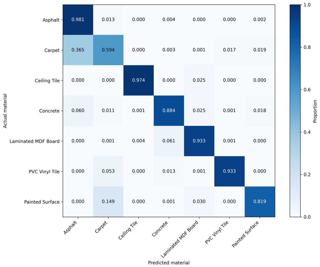
The class-specific performance of the final stacking classifier was further examined using the normalised confusion matrix shown in Figure 5. The diagonal elements represent the proportion of correctly classified points within each material class. Most classes achieved high recall, particularly Asphalt, Ceiling Tile, PVC Vinyl Tile, and Laminated MDF Board, whereas Carpet showed the lowest recall and therefore remained the most challenging material to classify.

The normalised confusion matrix in Figure 5 shows that most material classes were classified with high recall. Asphalt achieved the highest recall at 98.14%, followed by Ceiling Tile at 97.45%, PVC Vinyl Tile at 93.33%, and Laminated MDF Board at 93.28%. Concrete achieved a recall of 88.45%, while Painted Surface achieved 81.87%. Carpet was the most challenging class, with a recall of 59.42%.

The largest remaining confusion occurred between Carpet and Asphalt, with approximately 36.49% of Carpet points classified as Asphalt. Smaller proportions of Carpet points were classified as Painted Surface (1.88%) and PVC Vinyl Tile (1.73%). Other notable errors included approximately 14.94% of Painted Surface points classified as Carpet, 5.97% of Concrete points classified as Asphalt, 6.12% of Laminated MDF Board points classified as Concrete, and 5.30% of PVC Vinyl Tile points classified as Carpet.

These results indicate that the proposed multiscale feature set provides strong discrimination for most material classes, but some overlap remains in the combined radiometric–geometric feature space. In particular, the lower recall for Carpet suggests that its Slope_SKL, Ra, and Rn distributions overlap with those of Asphalt for a portion of the test data. This class-specific behaviour is also reflected in the difference between the overall accuracy (90.44%) and balanced accuracy (87.42%), emphasising the importance of considering both aggregate and class-specific performance.

The ablation analysis provides a more direct assessment of feature contribution than model-specific importance scores. The results show that plane-residual roughness provides the largest improvement beyond the radiometric descriptor, while normal-variation roughness contributes additional complementary information when incorporated at multiple spatial scales. This supports the use of the combined multiscale radiometric–geometric representation rather than reliance on a single descriptor or a single neighbourhood scale.

An important advantage of the proposed approach is that it avoids reliance on illumination-dependent colour features. RGB- and HSV-derived descriptors may vary with illumination conditions, shadows, and image-acquisition settings [5]. In contrast, the proposed framework relies exclusively on TLS-derived radiometric and geometric descriptors. The results therefore demonstrate that effective construction-material discrimination can be achieved without incorporating image-based colour information.

The evaluation was performed using separate training and held-out test datasets, with class balancing applied only to the training data. The held-out test dataset retained its original class distribution and was not used during model selection or hyperparameter optimisation. Nevertheless, the results should be interpreted within the acquisition conditions represented by the present dataset. Although the data were obtained from real indoor and outdoor building surfaces, further validation using independent scan campaigns, additional buildings, scanner positions, material conditions, and environmental settings is required to establish broader transferability and generalisation.

From a computational perspective, feature extraction represents a substantial component of the workflow because multiscale neighbourhood searches, RANSAC plane fitting, surface-normal estimation, and roughness calculation are performed for individual point-cloud neighbourhoods. KD-tree-based neighbourhood searches and parallel processing were used to support processing of the large TLS datasets. The AutoML optimisation was performed using a 900 s computational budget with three-fold cross-validation and macro F1-score as the optimisation metric. Future work should investigate further computational improvements, including spatial downsampling, parallel neighbourhood processing, and tiled point-cloud processing, and should report detailed runtime and memory requirements for large-scale construction scenes.

5. Conclusions

This study presented a TLS-only framework for construction material classification using a reflectance-related radiometric descriptor together with multiscale geometric roughness features. The radiometric information was represented by the local intensity–geometry regression descriptor, Slope_SKL, while plane-residual roughness Ra and normal-variation roughness Rn were calculated using cube neighbourhoods with side lengths of 0.10, 0.20, and 0.30 m. The resulting seven-feature representation therefore combined radiometric response with complementary measures of local surface magnitude and directional variation.

Model development was performed using FLAML with three-fold cross-validation and macro F1-score as the optimisation metric. Class balancing was applied only to the training dataset, while the held-out test dataset retained its original class distribution. The final stacking classifier achieved an overall accuracy of 90.44%, balanced accuracy of 87.42%, and macro F1-score of 87.85% on 1,296,822 held-out test points. These results reflect scan-position-separated held-out validation within the same general study area and should not be interpreted as evidence of cross-site generalisation.

The ablation analysis confirmed that geometric roughness provides substantial discriminatory information beyond the radiometric descriptor. Plane-residual roughness contributed the largest improvement, while multiscale normal-variation roughness provided additional complementary information. Class-specific evaluation showed that most materials were well-discriminated, although Carpet remained the most challenging class because of confusion with Asphalt.

Overall, the findings demonstrate that combining a reflectance-related radiometric descriptor with multiscale plane-residual and normal-variation roughness provides an effective TLS-only representation for construction material classification. The framework achieved strong performance without relying on RGB- or HSV-based colour information, supporting its potential for automated construction monitoring and digital twin applications.

Future work should focus on independent validation across additional buildings, scan campaigns, material conditions, and acquisition geometries. It should also investigate material-specific neighbourhood scales for Ra and Rn calculation, with the aim of identifying the cube side length that best represents the characteristic surface structure of each material and potentially improves class discrimination.