A Graded Evaluation Method for Construction Quality of Prefabricated Beam Bridges Based on Manifold Learning and Probability Distributions

Abstract

This study aims to construct a graded evaluation method for the construction quality of Highway Prefabricated Beam Bridges, in order to support refined quality control beyond the traditional “qualified/unqualified” judgment. Existing evaluation methods have difficulty effectively distinguishing quality differences within the qualified range, may cause redundant calculations for indicator information with non-linear correlations, are susceptible to the influence of outlier expert judgments, and may mask local critical defects when adopting linear weighted aggregation. This paper uses historical quality inspection and expert evaluation records from 50 prefabricated beam bridges to validate the proposed method. Experimental results show that the proposed method achieves an RMSE of 1.24, outperforming the traditional AHP method (1.79) and the equal-weight method (2.52). Five-fold grouped cross-validation at the bridge level gave an RMSE of 1.2180 ± 0.0802 and an R² of 0.9536. It can provide accurate intelligent decision support for quality and safety control during the construction of Highway Prefabricated Beam Bridges, and promotes the digital upgrade of quality management in the construction industry. The proposed framework can be integrated into a digital construction quality management platform to support bridge quality ranking and early warning of safety-critical defects. The originality of this paper lies in the integration, within a unified evaluation framework, of continuous score conversion based on probability distributions, manifold-learning-based redundancy correction for indicators, geometrically median-based robust fusion of expert weights, and a threshold-triggered risk-sensitive weight adjustment mechanism.

1. Introduction

Highway Prefabricated Beam Bridges (HPBB) are characterized by factory-based precast production and on-site assembly. They offer short construction periods, high quality consistency, and minimal traffic disruption, and have therefore become one of the mainstream structural forms in highway network construction [1,2,3]. Establishing accurate and objective methods for evaluating finished product quality is of significant theoretical value and engineering importance for ensuring the safe operation of bridges throughout their service life and for enabling data-driven quality decision-making [4,5,6].

Existing bridge quality evaluation methods fall into three categories: specification-based inspection, the Analytic Hierarchy Process (AHP), and intelligent evaluation methods.

Specification-based inspection follows national and industry standards. It checks, through on-site measurements, whether each quality parameter reaches the qualified level. This approach produces objective results and follows transparent procedures. However, it only provides a binary “pass/fail” judgment. Evaluation results are typically oriented toward meeting the qualified standard, and there is little discrimination within the qualified range. It is difficult to quantify the influence of individual indicators on overall performance or to reflect the intrinsic coupling relationships among indicators. Moreover, in large-scale bridge construction quality control, specification-based inspection alone cannot provide comprehensive quality ranking or risk classification information, and thus cannot meet the current demands of automation and intelligent development in HPBB.

The Analytic Hierarchy Process (AHP) decomposes complex decision problems into a hierarchy of goal, criteria, and alternative layers. It uses pairwise comparison matrices to quantify the relative importance of factors, thereby enabling comprehensive consideration of all influencing factors in the overall evaluation result. For example, Zhou D used AHP to determine the weights of factors in bridge thick plates and assigned quality grades based on evaluation scores [7]. Darban S adopted AHP to evaluate bridge quality based on weights and scores given by experts for major bridge indicators [8]. However, the weights in AHP rely on subjective expert judgments. Differences in preferences among experts lead to inconsistent weight assignments, which limits the generalisability of the evaluation results [9]. To reduce errors introduced by subjective judgments, Jin R integrated the CRITIC method and TOPSIS with traditional AHP, achieving accurate bridge quality evaluation by calculating the ideal solution of indicator weights [10]. Shu J proposed a fusion evaluation method based on evidence credibility, building on traditional fuzzy AHP, and used preprocessing correction to prevent some indicators from being overlooked [11]. Nevertheless, large-scale databases typically contain scores from multiple experts, each with different scoring tendencies and weight preferences. AHP averages expert opinions arithmetically, which inevitably makes it highly sensitive to outlier judgments; an extreme preference from a single expert can significantly distort the consensus weights. In addition, the traditional weighted average evaluation framework linearly superimposes indicator scores. When a critical indicator receives a very low score, its contribution is easily diluted by other high-scoring indicators, so that the composite score fails to reflect local severe defects. Yet quality problems in critical bridge components may lead to overall structural failure and cause extremely serious accidents.

With the rapid development of machine learning and artificial intelligence, intelligent evaluation methods have made notable progress in bridge quality assessment [12,13]. Compared with traditional manual approaches, intelligent methods learn weights from large datasets and are used to monitor structural conditions and predict degradation in HPBB, thereby avoiding overall structural failure caused by quality exceedances in key parts [14,15]. For example, Recurrent Neural Networks (RNNs) and Long Short-Term Memory networks (LSTMs) have been applied to time-series prediction of bridge component degradation [16]. Shen C used LSTM to predict bridge conditions with 95% accuracy [17]. Concepcion R S combined principal component analysis with multilayer artificial neural networks for intelligent evaluation [18]. Alsharqawi M proposed a method using K-means clustering to objectively determine condition rating thresholds; while this reduced the uncertainty of manually set thresholds, the maximum accuracy was only 81% [19]. Malekly H adopted a fuzzy comprehensive evaluation method that incorporated expert knowledge and experience to handle the large amount of subjective or fuzzy data in bridge quality evaluation [20]. Jiang C used surface damage and neural networks to evaluate the transverse connection and durability of hollow slab bridges, but the output was limited to scores for hinge joints and beams, with a prediction error of 15% [21]. Xia Y proposed an AI-based method for regional bridge condition assessment, with an accuracy not exceeding 85% [22]. The reasons for the insufficient accuracy of the above methods are twofold. On the one hand, non-linear dependencies commonly exist among multi-level quality indicators, but researchers have not adequately accounted for the intrinsic geometric dependencies among indicators. This leads to double-counting of information from the same quality dimension, thereby biasing evaluation results. On the other hand, in the measured results, most indicators are concentrated at the highest grade, providing little reference value. For example, in the technical requirement for clay content in fine aggregates, contents below 1.0%, 3.0%, and 5.0% correspond to Classes I, II, and III, respectively, yet all measured results in the original records across bridge samples were Class I. This phenomenon arises from strict quality control requirements: when an indicator fails, the material is reconstructed to meet the highest technical standard. From both quality management and economic perspectives, this grading approach is reasonable. However, when a more nuanced quality assessment is needed, discrete and highly concentrated evaluation results lack discrimination. Simple grading ignores the specific mapping relationship between measured data and indicator evaluation indices, while fuzzy processing loses important information, making it difficult for intelligent methods to accurately extract weights. More importantly, the bridge construction quality evaluation in the current transportation industry has long been oriented toward a “qualified” boundary. Quality differences above the qualified level lack effective quantification, and refined quality grading remains a common industry challenge. Whether by discrete grading or fuzzification, both approaches sacrifice original measurement information, which fundamentally limits further improvement in grading precision.

To address the above problems, this paper proposes a graded evaluation method for the construction quality of HPBB based on manifold learning and probability distributions. Following the construction process of HPBB, we construct a four-level quality evaluation index system. We propose an indicator score transformation method based on the two-point distribution and the two-sided cumulative probability of the normal distribution, which maps discrete grades to continuous scores and eliminates information loss in traditional discrete grading. We formulate multi-expert weight fusion as a geometric median optimization on the probability simplex, and introduce expert confidence weighting based on a consistency index to robustly suppress outlier judgments. Based on safety thresholds, we design a piecewise weight incentive model that, when an indicator score falls below a preset threshold, activates an exponential incentive function to non-linearly amplify its weight share in the comprehensive score. While maintaining overall evaluation robustness, this local weight sharpening enables precise focus on extremely low scores, thereby facilitating timely detection of major quality and safety hazards. Finally, we calculate comprehensive scores for HPBB using the trained weights and scores, achieving an intelligent comprehensive evaluation of finished product quality.

The core innovations of this method include:

• A score transformation method based on the two-point distribution and the two-sided cumulative probability of the normal distribution, which maps discrete indicator grades to continuous scores and refines the differentiation of quality differences among indicators.
• The Isomap algorithm extracts the intrinsic geometric structure of indicator data, and a manifold-distance-based redundant weight attenuation mechanism eliminates double-counting caused by non-linear dependencies among indicators.
• Multi-expert weight fusion is formulated as a geometric median optimization problem on the probability simplex, and the Weiszfeld algorithm iteratively solves for consensus weights, suppressing the interference of outlier judgments.
• A threshold-triggered weight incentive mechanism non-linearly amplifies the weights of indicators whose scores approach safety thresholds, ensuring that local low scores are reflected in the comprehensive evaluation and thereby improving the identification capability for potential quality risks.

2. Evaluation Method Design

2.1. Evaluation System Construction

This evaluation system is primarily developed for prefabricated concrete beam bridges, excluding those made of steel, timber, or other materials. Following the construction process of HPBB, which comprises two phases—factory prefabrication and on-site assembly—the evaluation indicators are classified into two major categories: prefabricated component quality and installation quality. A four-level quality evaluation index system is thus established, consisting of 2 first-level indicators, 7 second-level indicators, 38 third-level indicators, and 36 fourth-level indicators (some third-level indicators contain fourth-level sub-indicators).

Let the set of first-level indicators be $=\{C_1,C_2,\dots ,C_K\}$, with a total of K first-level indicators. Each first-level indicator $C_k$ has $m_k$ second-level indicators, denoted as ${\mathcal{B}}_{\mathrm{k}}=\left\{B_{k1},B_{k2},\dots ,B_{k{m}_k}\right\}$. Each second-level indicator $B_{kj}$ has $n_{kj}$ third-level indicators, denoted as ${\mathcal{I}}_{kj}=\left\{I_{kj1},\dots ,I_{kj{n}_{kj}}\right\}$. Some third-level indicators $I_{kjl}$ contain $p_{\mathrm{k}\mathrm{j}\mathrm{l}}$ fourth-level sub-indicators (when $p_{kjl}$, there are no fourth-level sub-indicators), denoted as ${\mathcal{Q}}_{\mathrm{k}\mathrm{j}\mathrm{l}}=\left\{Q_{kjl1},\dots ,Q_{kjl{p}_{kjl}}\right\}$. The total number of bottom-level indicators (third-level indicators without fourth-level sub-indicators or fourth-level indicators) is denoted as M. The scores of all bottom-level indicators fall within [0, 100]. The evaluation system is presented in Table 1.

Table 1. Evaluation System.

First-Level Indicator	Second-Level Indicator	Third-Level Indicator	Fourth-Level Indicator
Precast Component Quality (PCQ)	Precast Pier Column (PPC)	Concrete Compressive Strength (MPa)	—
		Cross-Sectional Dimensions (mm)	—
		Height (mm)	—
		Flatness (mm)	—
		Bearing Pad Stone (mm)	Position
			Dimensions
			Precast Anchor Hole Position
		Embedded Parts (mm)	Grouting Sleeve/Metal Corrugated Pipe Center Position
			Reserved Steel Bar Position
			Reserved Steel Bar Exposure Length
	Precast Cap Beam (PCB)	Concrete Compressive Strength (MPa)	—
		Cross-Sectional Dimensions (mm)	—
		Height (mm)	—
		Flatness (mm)	—
		Bearing Pad Stone (mm)	Position
			Dimensions
			Precast Anchor Hole Position
		Embedded Parts (mm)	Grouting Sleeve/Metal Corrugated Pipe Center Position
			Reserved Steel Bar Position
			Reserved Steel Bar Exposure Length
	Precast Girder (PCG)	Concrete Compressive Strength (MPa)	—
		Girder Length (mm)	Total Length
			End Length
		Cross-Sectional Dimensions (mm)	Box Girder Top Width
			Box Girder Bottom Width
			Other Girder/Slab Dry Joint (Flange/Plate)
			Other Girder/Slab Wet Joint (Flange/Plate)
			Box Girder Height
			Other Girder/Slab Height
			Top slab/Bottom slab/web or rib thickness
		Flatness (mm)	—
		Cross Beam and Embedded Part Position (mm)	—
		Cross Slope (%)	—
		Cable-Stayed Anchor Surface	Anchor Point Coordinates (mm)
			Anchor Surface Angle (°)
Installation Quality (IQ)	Pier and Column Installation (PCI)	Axis Deviation (mm)	—
		Top Surface Elevation (mm)	—
		Full Height Verticality	—
		Segment-to-Segment Misalignment (mm)	—
		Wet Joint Concrete Strength (MPa)	—
	Precast Girder/Plate Installation (PGI)	Concrete Compressive Strength (MPa)	—
		Girder Length (mm)	Total Length
			Segment Length
		Cross-Sectional Dimensions (mm)	Box Girder Top Width
			Box Girder Bottom Width
			Other Girder/Slab Dry Joint (Flange/Plate)
			Other Girder/Slab Wet Joint (Flange/Plate)
			Box Girder Height
			Other Girder/Slab Height
			Top slab, bottom slab, web, or beam rib thickness
		Flatness (mm)	—
		Cross Beam and Embedded Part Position (mm)	—
		Cross Slope (%)	—
	Girder/Plate Installation (GPI)	Bearing Center Deviation (mm)	Girder
			Plate
		Girder/Plate Top Elevation (mm)	—
		Adjacent Girder/Plate Top Elevation Difference (mm)	—
	Span-by-Span Girder Assembly (SGA)	Axis Deviation (mm)	—
		Adjacent Segment Joint Misalignment (mm)	Top Surface
			Bottom/Side Surface
		Segment Assembly Vertical Joint Width (mm)	—
		Girder Length (mm)	—
		Bearing Center Deviation (mm)	—

2.2. Scoring Method

For indicators whose valid ranges are of the form {≥, >, <, ≤}, scoring follows a two-point distribution: measurements within the valid range receive 100 points, while those outside receive 0 points.

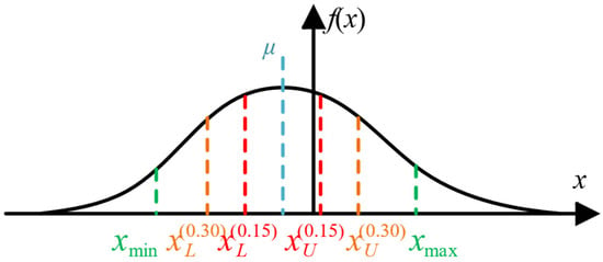
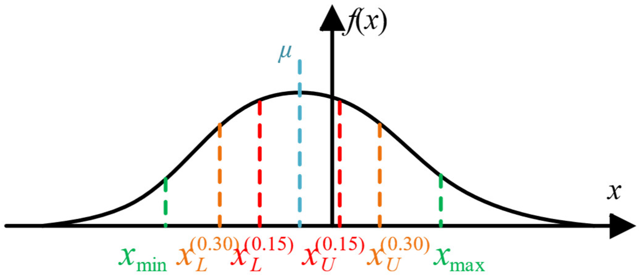
For bottom-level indicators whose valid range is a finite interval, a two-sided piecewise-normalized truncated normal model (Figure 1) is constructed over $\left[x_{\mathrm{m}\mathrm{i}\mathrm{n}},x_{\mathrm{m}\mathrm{a}\mathrm{x}}\right]$ using the mean $\mu$ and standard deviation $\sigma$ estimated exclusively from the training bridges. Unlike a conventional normal distribution defined over the entire real line, the proposed model normalizes the total probability within the valid interval to 1 and treats $\mu$ as the probability center, such that the probability masses over the left-side interval $\left[x_{\mathrm{m}\mathrm{i}\mathrm{n}},\mu \right]$ and the right-side interval $\left[\mu ,x_{\mathrm{m}\mathrm{a}\mathrm{x}}\right]$ are both 0.5. Measurements outside the valid interval are excluded from the within-range probabilistic grading procedure and are directly judged as unqualified, with a score of 0.

Figure 1. Schematic diagram of the truncated normal model.

Let $f_0\left(x\right)$ denote the underlying normal probability density function parameterized by $\mu$ and $\sigma$:

$$f_0\left(x\right)={\displaystyle \frac{1}{\sigma \sqrt{2\pi }}}\mathrm{e}\mathrm{x}\mathrm{p}\left[-{\displaystyle \frac{{\left(x-\mu \right)}^2}{2{\sigma }^2}}\right]$$

(1)

Let $\Phi \left(\cdot \right)$ denote the cumulative distribution function of the standard normal distribution. The probability masses of the underlying normal curve within the valid intervals on the left and right sides of the mean are respectively defined as

$$A_L=\Phi \left(0\right)-\Phi \left({\displaystyle \frac{x_{\mathrm{m}\mathrm{i}\mathrm{n}}-\mu }{\sigma }}\right)$$

(2)

$$A_U=\Phi \left({\displaystyle \frac{x_{\mathrm{m}\mathrm{a}\mathrm{x}}-\mu }{\sigma }}\right)-\Phi \left(0\right)$$

(3)

Accordingly, the two-sided piecewise-normalized probability density function over the valid interval is defined as:

$$f_B\left(x\right)=\left\{\begin{array}{ll}{\displaystyle \frac{f_0\left(x\right)}{2A_L}},& x_{\mathrm{m}\mathrm{i}\mathrm{n}}\le x\le \mu \\ {\displaystyle \frac{f_0\left(x\right)}{2A_U}},& \mu <x\le x_{\mathrm{m}\mathrm{a}\mathrm{x}}\\ 0,& x<x_{\mathrm{m}\mathrm{i}\mathrm{n}}\hspace{0.25em}\mathrm{or}\hspace{0.25em}x>x_{\mathrm{m}\mathrm{a}\mathrm{x}}\end{array}\right.$$

(4)

This probability density function satisfies

$${\int }_{x_{\mathrm{m}\mathrm{i}\mathrm{n}}}^{\mu }{f}_B\left(x\right)\hspace{0.17em}\mathrm{d}x={\int }_{\mu }^{x_{\mathrm{m}\mathrm{a}\mathrm{x}}}{f}_B\left(x\right)\hspace{0.17em}\mathrm{d}x={\displaystyle \frac{1}{2}}$$

(5)

$${\int }_{x_{\mathrm{m}\mathrm{i}\mathrm{n}}}^{x_{\mathrm{m}\mathrm{a}\mathrm{x}}}{f}_B\left(x\right)\hspace{0.17em}\mathrm{d}x=1$$

(6)

Let the one-sided cumulative probability parameter $0<\alpha \le 0.5$ denote the target probability accumulated from the mean toward either boundary. Let $x_L^{\left(\alpha \right)}$ and $x_U^{\left(\alpha \right)}$ denote the corresponding probability boundary points on the left and right sides of the mean, respectively.

$$P \left(x_L^{\left(\alpha \right)}<X<\mu \right)=P \left(\mu <X<x_U^{\left(\alpha \right)}\right)=\alpha$$

(7)

$$P \left(x_L^{\left(\alpha \right)}<X<x_U^{\left(\alpha \right)}\right)=2\alpha$$

(8)

The corresponding boundary points can be expressed as:

$$x_L^{\left(\alpha \right)}=\mu +\sigma {\Phi }^{-1} \left[\Phi \left(0\right)-2\alpha A_L\right]$$

(9)

$$x_U^{\left(\alpha \right)}=\mu +\sigma {\Phi }^{-1} \left[\Phi \left(0\right)+2\alpha A_U\right]$$

(10)

where ${\Phi }^{-1}\left(\cdot \right)$ denotes the inverse cumulative distribution function of the standard normal distribution.

When $\alpha =0.15$, the boundary points are denoted by $x_L^{\left(0.15\right)}$ and $x_U^{\left(0.15\right)}$, and the two-sided cumulative probability between them is 30%:

$$P \left(x_L^{\left(0.15\right)}<X<x_U^{\left(0.15\right)}\right)=0.30$$

(11)

When $\alpha =0.30$, the boundary points are denoted by $x_L^{\left(0.30\right)}$ and $x_U^{\left(0.30\right)}$, and the two-sided cumulative probability between them is 60%:

$$P \left(x_L^{\left(0.30\right)}<X<x_U^{\left(0.30\right)}\right)=0.60$$

(12)

When $\alpha =0.50$, the two boundary points reduce to the lower and upper limits of the valid interval:

$$x_L^{\left(0.50\right)}=x_{\mathrm{m}\mathrm{i}\mathrm{n}}, x_U^{\left(0.50\right)}=x_{\mathrm{m}\mathrm{a}\mathrm{x}}$$

(13)

$$P \left(x_{\mathrm{m}\mathrm{i}\mathrm{n}}\le X\le x_{\mathrm{m}\mathrm{a}\mathrm{x}}\right)=1$$

(14)

Table 2 lists the evaluation grades of the secondary indicators classified by the two-sided probability intervals of the normal distribution.

Table 2. Indicator Evaluation Grades and Score Intervals.

Grade	Indicator Value Interval	Score Interval
Excellent	$x_L^{\left(0.15\right)}\le x\le x_U^{\left(0.15\right)}$	[90, 100]
Good	$x_L^{\left(0.30\right)}\le x<x_L^{\left(0.15\right)}$ or $x_U^{\left(0.15\right)}<x\le x_U^{\left(0.30\right)}$	[75, 90)
Qualified	$x_{\mathrm{m}\mathrm{i}\mathrm{n}}\le x<x_L^{\left(0.30\right)}$ or $x_U^{\left(0.30\right)}<x\le x_{\mathrm{m}\mathrm{a}\mathrm{x}}$	[60, 75)
Unqualified	$x<x_{\mathrm{m}\mathrm{i}\mathrm{n}}$ or $x>x_{\mathrm{m}\mathrm{a}\mathrm{x}}$	[0, 60)

For any partition interval $\left[x_a,x_b\right]$, with the probability density range within the interval being $\left[f_{\mathrm{m}\mathrm{i}\mathrm{n}},f_{\mathrm{m}\mathrm{a}\mathrm{x}}\right]$, the scores for bottom-level indicators (third-level indicators $I_{kjl}$ and fourth-level indicators $Q_{kjls}$ are calculated as:

$$t_{kjl}=S_{\mathrm{l}\mathrm{o}\mathrm{w}}+\left(S_{\mathrm{h}\mathrm{i}\mathrm{g}\mathrm{h}}-S_{\mathrm{l}\mathrm{o}\mathrm{w}}\right)·{\displaystyle \frac{f\left(x\right)-f_{\mathrm{m}\mathrm{i}\mathrm{n}}}{f_{\mathrm{m}\mathrm{a}\mathrm{x}}-f_{\mathrm{m}\mathrm{i}\mathrm{n}}}}$$

(15)

$$v_{kjls}=S_{\mathrm{l}\mathrm{o}\mathrm{w}}+\left(S_{\mathrm{h}\mathrm{i}\mathrm{g}\mathrm{h}}-S_{\mathrm{l}\mathrm{o}\mathrm{w}}\right)·{\displaystyle \frac{f\left(x\right)-f_{\mathrm{m}\mathrm{i}\mathrm{n}}}{f_{\mathrm{m}\mathrm{a}\mathrm{x}}-f_{\mathrm{m}\mathrm{i}\mathrm{n}}}}$$

(16)

The grade boundaries are the probability quantiles defined above: $x_L^{\left(0.15\right)}, x_U^{\left(0.15\right)}$, $x_L^{\left(0.30\right)}$, $x_U^{\left(0.30\right)}$, $x_{\mathrm{m}\mathrm{i}\mathrm{n}}$, and $x_{\mathrm{m}\mathrm{a}\mathrm{x}}$. $t_{kjl}$ and $v_{kjls}$ are the final evaluation scores for the third-level indicator $I_{kjl}$ (without fourth-level sub-indicators) and the fourth-level indicator $Q_{kjls}$, respectively. $S_{\mathrm{l}\mathrm{o}\mathrm{w}}$ and $S_{\mathrm{h}\mathrm{i}\mathrm{g}\mathrm{h}}$ are the lower and upper bounds of the score limits of the relevant grade interval. f(x) is the truncated-normal density at the measured value; and $f_{\mathrm{m}\mathrm{i}\mathrm{n}}$ and $f_{\mathrm{m}\mathrm{a}\mathrm{x}}$ are the minimum and maximum densities within that interval. The expressions yield the scores of third-level indicators without sub-indicators and of fourth-level indicators, respectively.

2.3. Evaluation Model Design

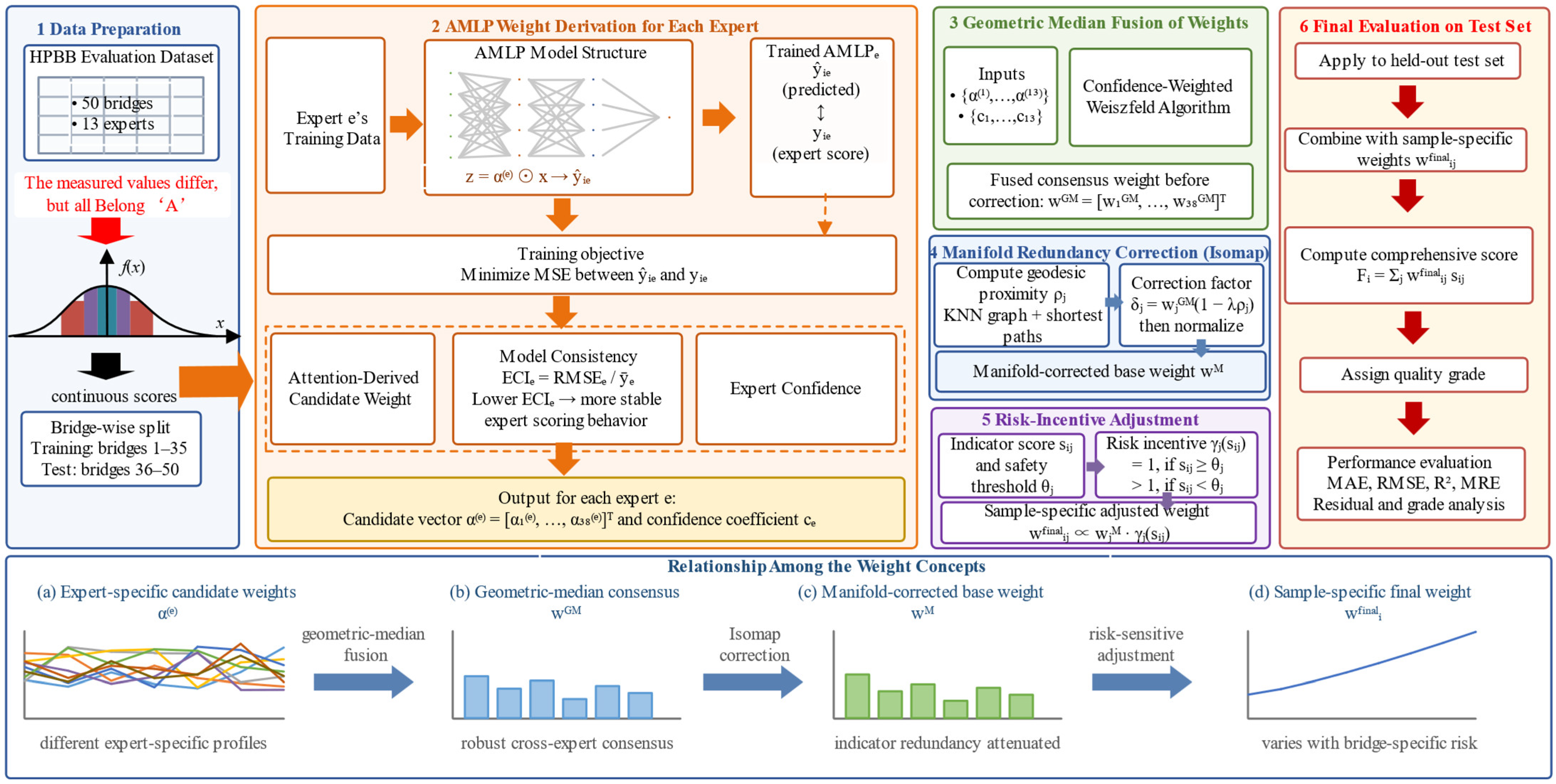
The evaluation model follows four progressive stages: candidate-importance generation, multi-expert fusion, redundancy correction, and risk-sensitive adjustment. Its overall workflow is shown in Figure 2. Figure 2 illustrates the representative hold-out workflow; the same training pipeline is reconstructed fold by fold during grouped cross-validation. First, an expert-specific attention-enhanced multilayer perceptron (AMLP) derives a candidate initial importance vector from training scores and the corresponding expert ratings. Second, the expert-specific candidate vectors are fused by a confidence-weighted geometric median. Third, Isomap-based redundancy correction is applied to the third-level analysis weights. Finally, a threshold-triggered incentive adjusts the third-level weights for each bridge according to its observed risk state.

Figure 2. Flowchart of the proposed evaluation model.

2.3.1. Attention-Derived Candidate Initial Importance via an Attention-Enhanced Neural Network

We employ an Attention-enhanced Multilayer Perceptron (AMLP) to derive data-driven initial importance coefficients for indicators at all levels. The Softmax-normalized vector acts as a non-negative gating vector, constrained to the probability simplex. Because the gated features subsequently undergo fully connected layers and nonlinear activations, the Softmax coefficients do not directly quantify each indicator’s actual contribution to the AMLP output.

$$\widehat{\mathrm{y}}=f(\alpha \odot x;\Theta )$$

(17)

Here, α controls the relative amplitude of the input features entering the downstream network, whereas the output attribution also depends on Θ, the downstream parameters and activation states. Therefore, α has an input-gating interpretation rather than an exact output-contribution interpretation.

To evaluate whether the candidate coefficients provide a reasonable global importance ordering after accounting for the downstream fully connected layers, whole-network Integrated Gradients are calculated for each expert-specific AMLP. A zero-score vector is adopted as the baseline because it represents the common lower boundary of the normalized quality indicators.

$$x_i^{(t)}=x^{ref}+{\displaystyle \frac{t}{T}}(x_i-x^{ref})$$

(18)

$${IG}_{ij}=(x_{ij}-{x_j}^{ref}){\displaystyle \frac{1}{T}}{\displaystyle \sum _{t=1}^T}{\displaystyle \frac{\partial f(x_i^{(t)})}{\partial x_j}}$$

(19)

$$I_j^{IG}={\displaystyle \frac{{\displaystyle {\sum }_{i=1}^N}abs({IG}_{ij})}{{\displaystyle {\sum }_{l=1}^M}{\displaystyle {\sum }_{i=1}^N}abs({IG}_{il})}}$$

(20)

Ordering consistency is assessed by computing the Spearman rank correlation and the overlap of the top-ranked indicators between the candidate coefficient vector and the Integrated Gradients importance vector. The input layer receives the score vector $\mathrm{x}\in {\mathbb{R}}^M$ of the M bottom-level indicators (third-level indicators without fourth-level sub-indicators or fourth-level indicators). Above the input layer, we set an indicator attention layer. This layer weights the input features using a learnable parameter vector $\mathrm{a}\in {\mathbb{R}}^M$. The attention scores are normalized via Softmax to produce:

$$\alpha =Softmax\left(a\right)\in {\Delta }^{M-1}, z=\alpha \odot x$$

(21)

Here, α is the normalized attention-gating coefficient vector after Softmax, ⊙ denotes the element-wise (Hadamard) product, $z\in {\mathbb{R}}^M$ is the attention-weighted feature vector, ${\Delta }^{M-1}$ is the $\left(M-1\right)$-dimensional probability simplex, and $x\in {\mathbb{R}}^M$ is the input bottom-level indicator score vector.

The weighted features z are passed through several fully connected hidden layers. The final output layer produces the predicted comprehensive quality score $\widehat{F}\in \left[0,100\right]$.

The network is trained by gradient descent with the following loss function:

$$\mathcal{L}={\displaystyle \frac{1}{N}}{\displaystyle \sum _{i=1}^N}{\left({\widehat{F}}_i-F_i\right)}^2$$

(22)

Here, N is the total number of training samples, ${\widehat{F}}_i$ is the predicted comprehensive quality score for the i-th sample, and $F_i$ is the true expert comprehensive score for the i-th sample.

After training, the normalized attention-gating coefficient vector $\mathsf{\alpha }\in {\Delta }^{M-1}$ provides the initial weights for all bottom-level indicators. Based on the attention-gating coefficients α, weights are aggregated according to the indicator hierarchy:

$$w_{kj}^{\left(0\right)}={\displaystyle \frac{{\alpha }_{kj}}{{\displaystyle {\sum }_{j^{\prime }=1}^{m_k}}{\alpha }_{k{j}^{\prime }}}}, W_k^{\left(0\right)}={\displaystyle \sum _{j=1}^{m_k}}{\alpha }_{kj}$$

(23)

For a third-level indicator $I_{kjl}$ containing fourth-level sub-indicators: the initial fourth-level weights are $u_{kjls}^{(0)}$ = ${\alpha }_{kjls}$/∑${\mathrm{s}}^{\prime }{\alpha }_{kjl{s}^{\prime }}$, and the third-level aggregation coefficient is ${\omega }_{kjl}^{(0)}$ = ∑$s{\alpha }_{kjls}$. For a third-level indicator without fourth-level sub-indicators: ${\omega }_{kjl}^{(0)}$ = ${\alpha }_{kjl}$. The initial third-level weight is $w_{kjl}^{(0)}$ = ${\omega }_{kjl}^{(0)}$/∑$l^{\prime }{\omega }_{kj{l}^{\prime }}^{(0)}$. The initial second-level weight is $W_{kj}^{(0)}$ = ∑$l{\omega }_{kjl}^{(0)}$/∑$j^{\prime }$ ∑$l^{\prime }{\omega }_{k{j}^{\prime }{l}^{\prime }}^{(0)}$. The initial first-level weights are ${\Omega }_k^{(0)}$.

2.3.2. Robust Multi-Expert Weight Fusion via Geometric Median

In the actual evaluation database, a total of E experts independently assign weights to indicators at all levels based on their engineering judgment. Taking third-level weights as an example: let the weight vector assigned by the e-th expert to the third-level indicators under second-level indicator B_kj be $w_{kj}^{(e)}$=($w_{kj1}^{(e)}$,…,$w_{kj{n}_{kj}}^{(e)}$)∈${\Delta }^{n_{kj}-1}$. Correspondingly, the E experts independently assign weights to second-level weights $W_{kj}$, fourth-level weights $u_{kjls}$, and first-level weights ${\Omega }_{\mathrm{k}}$. The probability simplex ${\Delta }^{m-1}$ is defined as:

$$k{w}_k^{\left(e\right)}=\left(w_{k1}^{\left(e\right)},\dots ,w_{k{m}_k}^{\left(e\right)}\right)\in {\Delta }^{m_k-1}{\Delta }^{m-1}\left(m-1\right)$$

(24)

$${\Delta }^{m-1}=\{w\in {\mathbb{R}}^m│\hspace{0.33em}{w}_j\ge 0,\hspace{0.33em}{\displaystyle {\sum }_{j=1}^m}{w}_j=1\}$$

(25)

Here, w is the weight vector, m is the number of indicators in the group, and $w_j$ is the weight component for the j-th indicator.

Different expert weights vary significantly, forming a discrete point cloud $\{w_k^{\left(1\right)},w_k^{\left(2\right)},\dots ,w_k^{\left(E\right)}\}$ on the simplex. We extract the optimal consensus weight vector ${\mathrm{w}}_k^{*}$ that minimizes the total deviation from all expert judgments.

The confidence coefficient ${ECI}_e$ assigned to expert e is calculated as:

$${ECI}_e= {\displaystyle \frac{\sqrt{\frac{1}{N_e} {\displaystyle {\sum }_{i=1}^{N_e}}{\left({F̂}_{e,i} - F_{e,i}\right)}^2}}{{F̄}_e}}$$

(26)

Here, $N_e$ is the number of training bridge samples scored by expert e, ${F̂}_{e,i}$ is the AMLP-predicted comprehensive score for expert e’s i-th sample using the weight structure learned from expert e’s data, $F_{e,i}$ is expert e’s actual comprehensive rating for that sample, and ${F̂}_{e,i}$ is the mean of expert e’s comprehensive ratings across their $N_e$ training samples.

The expert confidence weight α_e is calculated as:

$${\alpha }_e={\displaystyle \frac{exp\left(-\mu \cdot {ECI}_e\right)}{{\displaystyle {\sum }_{e^{\prime }=1}^E}exp\left(-\mu \cdot {ECI}_{e^{\prime }}\right)}}$$

(27)

Here, $\mu >0$ is a hyperparameter controlling the sensitivity of confidence assignment. When $C{R}_e=0$, expert judgment is perfectly consistent and the confidence is highest. As $C{R}_e$ increases, confidence decays exponentially.

We adopt the geometric median as a robust measure of central tendency for the multi-expert weights:

$$w_k^{*}=\underset{w\in {\Delta }^{m_k-1}}{argmin}\hspace{0.33em}f\left(w\right), f\left(w\right)={\displaystyle \sum _{e=1}^E}{\alpha }_e\cdot \parallel w-w_k^{\left(e\right)}{\parallel }_2$$

(28)

Here, ${\mathrm{w}}_k^{*}$ is the optimal consensus weight vector, f(w) is the objective function of the confidence-weighted sum of distances, αe is the confidence weight of the e-th expert, $w_k^{\left(e\right)}$ is the expert-specific AMLP-derived candidate vector, and $\parallel \cdot {\parallel }_2$ denotes the Euclidean norm.

The objective function f(w) is convex, and its minimizer is the confidence-weighted geometric median. We solve it using the Weiszfeld iterative algorithm with simplex projection:

$$\tilde{w}={\displaystyle \frac{{\displaystyle {\sum }_{e=1}^E}\frac{{\alpha }_e\cdot w_k^{\left(e\right)}}{\parallel w^{\left(t\right)}-w_k^{\left(e\right)}{\parallel }_2}}{{\displaystyle {\sum }_{e=1}^E}\frac{{\alpha }_e}{\parallel w^{\left(t\right)}-w_k^{\left(e\right)}{\parallel }_2}}}$$

(29)

Here, $\tilde{w}$ is the intermediate result of the Weiszfeld iteration, and w(t) is the current estimate at the t-th iteration.

$$w^{\left(t+1\right)}={\Pi }_{\Delta }\left(\tilde{w}\right)$$

(30)

Here, ${\Pi }_{\Delta }\left(\cdot \right)$ denotes the Euclidean projection operator onto the probability simplex. Iteration stops when $\parallel {\mathrm{w}}^{\left(t+1\right)}-{\mathrm{w}}^{\left(t\right)}{\parallel }_2<\epsilon$ ($\epsilon ={10}^{-6}$) or when the maximum iteration count is reached.

If a candidate vector coincides with the current iterate, a small subgradient perturbation is used to avoid division by zero. The same fusion procedure is applied to the first-level vector, the second-level groups, and the third-level groups, yielding the corresponding consensus weights.

2.3.3. Redundancy Correction of Indicator Weights via Manifold Learning

The consensus weights ${\mathrm{w}}_k^{*}$ obtained from multi-expert fusion are based on expert experience. They do not eliminate the double-counting caused by intrinsic geometric dependencies among indicators.

Traditional Euclidean distance measures the “apparent distance” between two points along a straight line. When data lie on a curved manifold, this straight-line distance crosses data-sparse “off-manifold” space and overestimates the true structural difference between two points. In contrast, the path length along the manifold surface—the geodesic nearest-neighbor distance—accurately reflects the actual proximity between two points along the data distribution manifold. When the geodesic distance between two indicators on this manifold is small, their quality scores exhibit a highly consistent response pattern across a large number of real bridge samples.

Taking third-level indicator redundancy correction as an example: Suppose a second-level indicator $B_{kj}$ governs $n_{kj}$ third-level indicators $I_{kjl}$ (represented by aggregated scores if they contain fourth-level sub-indicators), and the number of bridge samples is N. We construct the data matrix $X_{kj}\in {\mathbb{R}}^{N\times n_{kj}}$, where column vector $x_{\mathrm{l}}\in {\mathbb{R}}^N$ is the score vector of the l-th third-level indicator across all samples. We treat each third-level indicator as a point in the high-dimensional sample space ${\mathbb{R}}^N$ and use the Isomap algorithm to compute the geodesic nearest-neighbor distances among third-level indicators:

• Construct a K-nearest neighbor graph $G=\left(V,\mathcal{E}\right)$, where the node set is $V=\{{\mathrm{x}}_1,\dots ,{\mathrm{x}}_{m_k}\}$. Add an edge if $x_i$ is among the K nearest neighbors of ${\mathrm{x}}_j$, with edge weight equal to the Euclidean distance $\parallel {\mathrm{x}}_i-{\mathrm{x}}_j{\parallel }_2$.
• Compute the shortest path distances between all indicator pairs using Dijkstra’s algorithm on G, as an approximation of the manifold geodesic distances. This yields the geodesic distance matrix ${\mathrm{D}}_G^{\left(k\right)}\in {\mathbb{R}}^{m_k\times m_k}$.
• Select the indicator with the largest consensus weight within the group as the reference indicator: $r_k=\mathrm{a}\mathrm{r}\mathrm{g}{\mathrm{m}\mathrm{a}\mathrm{x}}_j{w}_{kj}^{*}$.
• For each other indicator $j\ne r_k$, compute its manifold geodesic proximity to the reference indicator:

$${\rho }_{kj}=exp \left(-{\displaystyle \frac{{\left[D_G^{\left(k\right)}\left(j,r_k\right)\right]}^2}{2{\sigma }^2}}\right), j\ne r_k; {\rho }_{k,r_k}=0$$

(31)

Here, ${\rho }_{kj}$ is the manifold geodesic proximity of the j-th indicator in group k to the reference indicator $r_k$, $D_G^{\left(k\right)}\left(j,r_k\right)$ is the shortest path distance between the j-th indicator and the reference indicator $r_k$, and ${\sigma }^2$ is the bandwidth parameter, set as ${\sigma }^2={\left[{\mathrm{m}\mathrm{e}\mathrm{d}\mathrm{i}\mathrm{a}\mathrm{n}}_{j\ne j^{\prime }}{D}_G^{\left(k\right)}\left(j,j^{\prime }\right)\right]}^2$.

Based on the indicator geodesic proximity ${\rho }_{kj}$, we attenuate the consensus weights:

$${\widehat{w}}_{kj}=w_{kj}^{*}\cdot \left(1-\lambda \cdot {\rho }_{kj}\right), \forall j\in \{1,\dots ,m_k\}$$

(32)

Here, ${\widehat{w}}_{kj}$ is the attenuated weight, $w_{kj}^{*}$ is the multi-expert fused consensus weight, and $\lambda \in \left(0,1\right)$ is the attenuation strength hyperparameter. The reference indicator $r_k$ maintains its original weight because ${\rho }_{k,r_k}=0$. Indicators with higher geodesic proximity to the reference indicator experience greater attenuation.

The attenuated weights are then normalized:

$${\overline{w}}_{kj}={\displaystyle \frac{{\widehat{w}}_{kj}}{{\displaystyle {\sum }_{j^{\prime }=1}^{m_k}}{\widehat{w}}_{k{j}^{\prime }}}}$$

(33)

Here, ${\overline{w}}_{kj}$ is the normalized corrected weight.

Apply the above procedure independently to each indicator group at all levels (third-level indicators within each $B_{kj}$, fourth-level indicators within each $I_{kjl}$, and second-level indicators within each $C_k$). We also apply an equivalent manifold correction to the top-level first-level weight vector ${\Omega }_k$, yielding the final corrected weights ${\tilde{\Omega }}_k^{*}$, ${\tilde{W}}_{kj}^{*}$, ${\tilde{w}}_{kjl}^{*}$, and ${\tilde{u}}_{kjls}^{*}$.

2.3.4. Threshold-Triggered Risk-Sensitive Weight Incentive Mechanism

In bridge structural safety evaluation, the engineering significance of scores varies non-symmetrically across score intervals. The comprehensive quality score F is graded as follows: F ≥ 90 (Excellent), 75 ≤ F < 90 (Good), 60 ≤ F < 75 (Qualified), and F < 60 (Unqualified). These grade boundaries are used for quality classification and are distinct from the indicator-specific safety threshold used in the risk-sensitive adjustment. Within the same quality grade, the same score difference has similar engineering implications. However, when an indicator score falls below its indicator-specific safety threshold, the same score difference indicates a fundamentally different safety state. In particular, under the traditional weighted average framework, an extremely low score in a critical indicator may be averaged out by high scores in other indicators. As a result, the comprehensive score may fail to reflect the existence of local severe defects. The threshold-triggered risk-sensitive weight incentive mechanism solves this problem. When an indicator score falls below a preset safety threshold, its weight share is automatically amplified.

The safety threshold ${\theta }_{kj}$ is set based on two sources of information:

(a)

The qualified grade boundary of 60 points adopted in the scoring system;

(b)

The empirical lower-tail boundary of the indicator-score distribution, defined as one standard deviation below the mean estimated from the training bridges only.

$${\theta }_{kj}=max\left\{{\theta }_{kj}^{\mathit{spec}},\hspace{0.33em}{\mu }_{j,k}^{\mathit{train}}-{\sigma }_{j,k}^{\mathit{train}}\right\}$$

(34)

Here, ${\theta }_{kj}$ is the safety threshold for the j-th indicator in group k, ${\theta }_{kj}^{\mathrm{spec}}$ is the qualified critical value specified by codes, ${\mu }_{kj}$ is the mean score of the indicator $I_{kj}$ in the training set, and ${\sigma }_{kj}$ is its standard deviation. ${\theta }_{kj}^{\mathit{spec}}$ is the engineering lower bound of the risk trigger and is set to 60 points in this study, corresponding to the Qualified–Unqualified boundary in the adopted scoring system; ${\mu }_{j,k}^{\mathit{train}}$ and ${\sigma }_{j,k}^{\mathit{train}}$ are the mean and standard deviation, respectively, of the corresponding indicator scores estimated exclusively from the training bridges.

We define the piecewise risk incentive function ${\gamma }_{kj}:\left[0,100\right]\to [1,+\mathrm{\infty })$ as:

$${\gamma }_{kj}\left(s\right)=1, s\ge {\theta }_{kj}$$

(35)

$${\gamma }_{kj}\left(s\right)=exp \left(\beta \cdot {\left({\displaystyle \frac{{\theta }_{kj}-s}{{\theta }_{kj}}}\right)}^{ \alpha }\right), s<{\theta }_{kj}$$

(36)

Here, ${\gamma }_{kj}\left(s\right)$ is the risk incentive coefficient for indicator $I_{kj}$ at score s, $\beta >0$ is the incentive intensity coefficient, α > 0 is the shape coefficient, ${\theta }_{kj}$ is the safety threshold.

This function has the following key properties:

• Continuity: At the threshold, ${\gamma }_{kj}\left({\theta }_{kj}\right)=\mathrm{e}\mathrm{x}\mathrm{p}\left(0\right)=1$. The incentive function is continuous and has no jump at the threshold. First bullet;
• Monotonicity: For $s<{\theta }_{kj}$, ${\gamma }_{kj}\left(s\right)$ increases monotonically as s decreases. A lower score receives a stronger incentive.
• Boundedness: When s = 0, ${\gamma }_{kj}\left(0\right)=\mathrm{e}\mathrm{x}\mathrm{p}\left(\beta \right)$. The incentive upper limit is $\mathrm{e}\mathrm{x}\mathrm{p}\left(\beta \right)$. By setting a reasonable β, we prevent incentive weights from becoming uncontrolled.
• Shape adjustability: When α = 1, the incentive grows linearly below the threshold; When α < 1, the growth near the threshold is faster; When α > 1, the growth near zero score is faster.

For all indicators in group k, based on the manifold-corrected weights ${\overline{w}}_{kj}$ and the current measured score $s_{kj}$, we compute the incentivized weights and then normalize:

$${\tilde{w}}_{kj}={\overline{w}}_{kj}\cdot {\gamma }_{kj}\left(s_{kj}\right)$$

(37)

$${\tilde{w}}_{kj}^{*}={\displaystyle \frac{{\tilde{w}}_{kj}}{{\displaystyle {\sum }_{j^{\prime }=1}^{m_k}}{\tilde{w}}_{k{j}^{\prime }}}}$$

(38)

Here, ${\tilde{w}}_{kj}$ is the incentivized weight, ${\overline{w}}_{kj}$ is the manifold-corrected weight, ${\gamma }_{kj}\left(s_{kj}\right)$ is the risk incentive coefficient at the measured score $s_{kj}$, and ${\tilde{w}}_{kj}^{*}$ is the final normalized bottom-level indicator weight after risk incentive.

Independently apply the equivalent risk incentive and normalization procedure to weights at all levels: third-level weights $w_{\mathrm{k}\mathrm{j}\mathrm{l}}$, fourth-level weights $u_{kjls}$, second-level weights $W_{kj}$, and first-level weights ${\Omega }_k$, using the corresponding level’s aggregated scores ($t_{kjl}$, $v_{kjls}$, $B_{kj}$, or $C_k$) as inputs to the incentive function.

For first-level indicators:

$${\dot{W}}_k={\overline{W}}_k\cdot {\Gamma }_k\left(C_k\right), {\dot{W}}_k^{*}={\displaystyle \frac{{\dot{W}}_k}{{\displaystyle {\sum }_{k^{\prime }=1}^K}{\dot{W}}_{k^{\prime }}}}$$

(39)

Here, ${\dot{W}}_k$ is the incentivized first-level weight, $\overline{W}$ is the manifold-corrected first-level weight, ${\Gamma }_k\left(\cdot \right)$ is the risk incentive function for the first-level indicator, $C_k$ is the score of the k-th first-level indicator, ${\dot{W}}_k^{*}$ is the normalized final first-level weight.

The complete mathematical expression is:

$$F_i={\Sigma }_{k=1}^K{W}_k·{\Sigma }_{g\in G_k}{w}_{kg}^{(2)}·{\Sigma }_{j=1}^{m_g}w{̃}_{gj}^{(3,i)}{s}_{igj}$$

(40)

Here, $W_k$ and $w_{kg}^{(2)}$ are the fixed first- and second-level consensus weights, $w{̃}_{gj}^{(3,i)}$ is the risk-adjusted third-level weight for bridge i, $s_{igj}$ is the corresponding third-level score, and $C_k$ is the set of second-level groups under first-level indicator k.

3. Experimental Results and Analysis

3.1. Dataset Partition and Score Transformation

The dataset originates from acceptance test records of 50 prefabricated beam bridges on different highway projects. Prefabricated components were manufactured by six separate standard beam factories in accordance with unified technical specifications, avoiding single-manufacturer data bias. The samples cover 16–30 m span T-beams, box girders and hollow slabs, covering all prefabrication and installation quality indicators in the established index system (Table 1). A total of 1862 precast girders, piers and cap beams were measured across all 50 bridges; the component measurement data were aggregated at the bridge level, and, within each data split, the statistical mean and standard deviation used for indicator-score calibration and safety-threshold determination were estimated exclusively from the training bridges. Original inspection files come from official road quality supervision archives, with 13 domain experts providing independent comprehensive scores for each bridge sample. Each bridge was independently scored by 13 experts with different engineering backgrounds, yielding 650 expert-evaluation records corresponding to 50 bridge samples. The dataset was partitioned into training and test sets by bridge number: the first 35 bridge samples (455 expert-evaluation records) formed the training set, and the remaining 15 bridge samples (195 expert-evaluation records) formed the test set. Throughout this paper, “bridge sample” refers to one of the 50 physical bridges, whereas “expert-evaluation record” refers to one expert’s evaluation of one bridge; therefore, the 650 records are clustered observations and are not treated as 650 independent bridge samples.

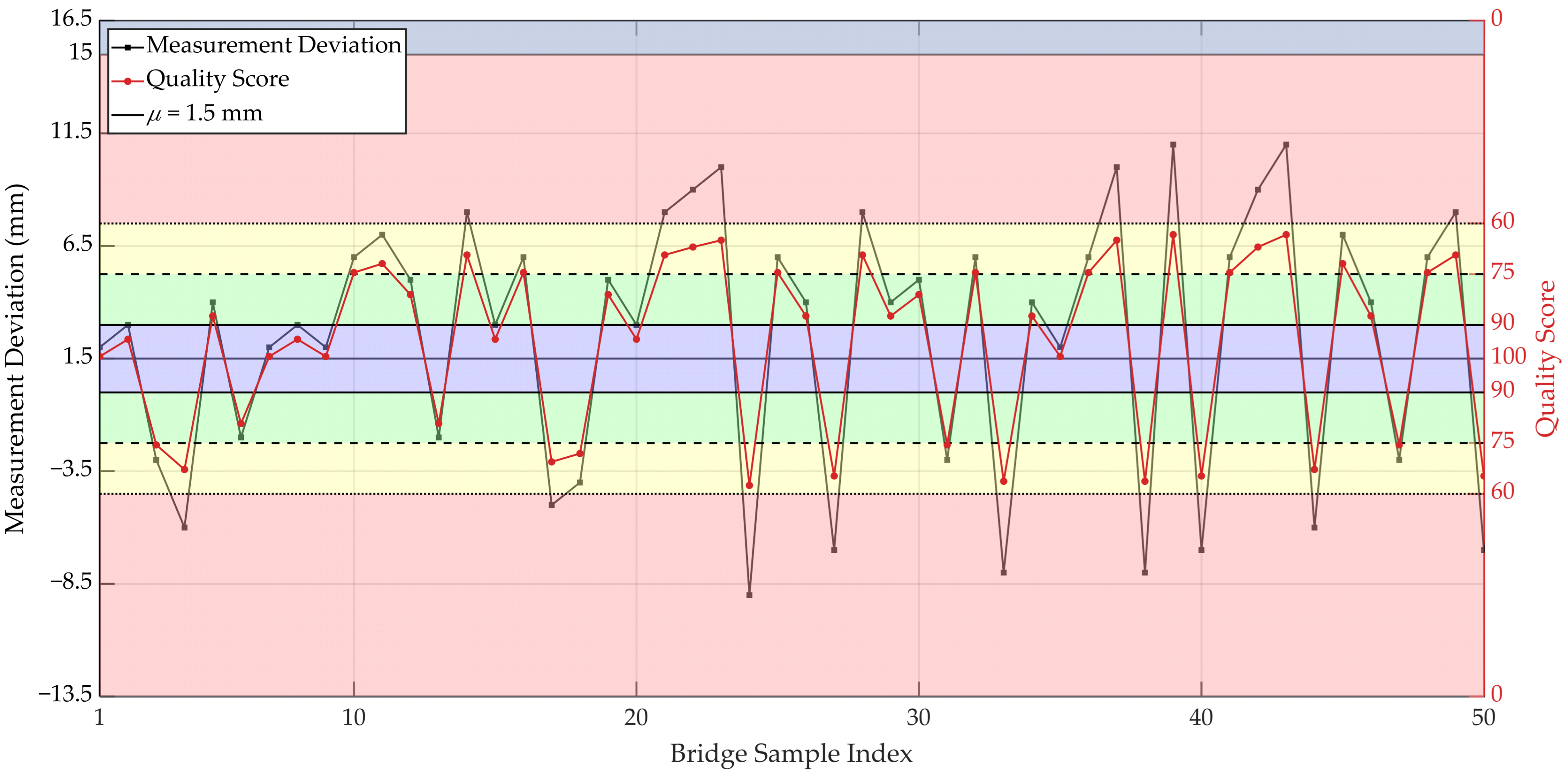
Taking the cross-sectional dimension indicator of precast cap beams under precast component quality as an example, the allowable deviation is ±15 mm. We used the average cross-sectional dimension of all precast cap beams in each bridge as the measured value. We collected 35 deviation values. The mean was μ = 1.5 mm, and the standard deviation was σ = 5.1 mm. Based on the normal distribution model, the boundary values and corresponding probability densities for each probability interval are shown in Table 3.

Table 3. Training-set cross-sectional-dimension deviations and truncated-normal parameters.

Parameter	Value
Deviation (mm)	2	3	−3	−6	4	−2
	2	3	2	6	7	5
	−2	8	3	6	−5	−4
	5	3	8	9	10	−9
	6	4	−7	8	4	5
	−3	6	−8	4	6
a	0.00	0.20	0.35	0.65	0.80	1.00
x	−15.0	−2.8	−0.45	3.49	5.82	15.0
f(x)	0.004	0.055	0.072	0.072	0.055	0.003
μ (mm)	1.5			σ (mm)	5.1

Under the traditional evaluation approach, all 50 bridges would be rated as “Qualified.” However, using the normal-distribution-based two-sided probability intervals, each bridge’s cross-sectional dimension evaluation was further differentiated. The corresponding scoring curve is shown in Figure 3.

Figure 3. Cross-Sectional Dimension Scores and Evaluation Intervals.

Under the traditional grading rule, all 50 measurements fall within the qualified interval. Using the scoring function calibrated from the 35 training bridges, each measurement was assigned a continuous score according to its location relative to μ = 1.5 mm. The same frozen transformation was applied to the 15 test bridges, ensuring a common score scale. The resulting scores were further classified as Excellent, Good, or Qualified using the 90, 75, and 60 points boundaries.

Because the 13 expert records associated with the same bridge are clustered observations of one engineering object, the bridge—not the individual expert record—was treated as the grouping unit. In addition to the representative 35/15 hold-out split used for prediction and residual visualization, five-fold bridge-level grouped cross-validation was used as the principal generalization assessment. The 50 bridges were divided into five mutually exclusive folds of 10 bridges, and all 13 records belonging to a bridge were retained in the same fold.

Within every outer fold, all data-dependent procedures were reconstructed using the training bridges only, including indicator-score calibration, expert-specific AMLP training, expert-confidence estimation, Weiszfeld geometric-median fusion, Isomap-based redundancy correction, and empirical risk-threshold determination. The fitted scoring functions and model parameters were then frozen and applied to the validation bridges. After the five outer folds were completed, the validation predictions were concatenated to form out-of-fold predictions for all 50 bridges. The mean of the 13 expert comprehensive ratings was used as the bridge-level reference score. Bridge-level MAE and RMSE were calculated within each fold.

To examine whether the estimated contributions of each module depended on a particular bridge assignment, the complete factorial ablation was evaluated using five independent repetitions of bridge-level grouped five-fold cross-validation. In each repetition, the 50 bridges were partitioned into five mutually exclusive folds. Within each outer training fold, the expert-specific AMLP models, expert confidence coefficients, fusion weights, Isomap correction parameters, and empirical risk thresholds were all reconstructed using only the training bridges. The 13 expert-specific AMLP models were trained once per outer fold, and the eight factorial configurations reused the resulting candidate weight vectors. After each complete repetition, the out-of-fold predictions from the five validation folds were pooled to compute MAE, RMSE, R², and MRE. The reported values are the mean and between-repetition standard deviation over the five complete repetitions.

3.2. Whole-Network Attribution Consistency and Initialization Sensitivity

The whole-network attribution analysis showed that the expert-specific Softmax candidate coefficients were positively and consistently associated with the Integrated Gradients importance after all downstream fully connected layers were considered. Across the 13 expert models, the mean Spearman rank correlation was 0.7490 ± 0.0681, ranging from 0.6555 to 0.8748; the mean Top-10 overlap was 6.92 out of 10, and the mean Pearson correlation was 0.7548. The global AMLP yielded a Spearman correlation of 0.7488 and a Top-10 overlap of 6/10. These results support the use of the Softmax vector as a candidate global ordering for initialization, while also confirming that it should not be interpreted as an exact feature-contribution vector.

The bounded-perturbation experiment further examined the dependence of the final evaluation on the candidate initialization. Table 4 summarizes the statistics from 100 Monte Carlo repetitions for each perturbation level. Under ±5%, ±10%, and ±20% perturbations, the mean test RMSE values were 1.2772, 1.2850, and 1.2838, respectively, all remaining on the same order of magnitude as the unperturbed baseline (1.2479), with a maximum deviation of only 0.0371; the mean MAE values were 1.0569, 1.0654, and 1.0653, again close to the baseline (1.0285). The mean final-weight Spearman correlations with the unperturbed model were 0.9446, 0.8624, and 0.7205, showing a decreasing trend with increasing perturbation magnitude, yet still maintaining a strong positive correlation even at ±20% perturbation. The mean prediction absolute differences (MAD) were 0.0315, 0.0473, and 0.0607 points, while the mean maximum prediction differences were 0.0735, 0.1241, and 0.1691 points. Most notably, the grade agreement rate was 100.00% for all perturbation levels, indicating that the relative ranking of the comprehensive scores was entirely unaffected. These results indicate that the subsequent fusion and correction procedures substantially reduce the dependence of the final evaluation on moderate uncertainty in the candidate initialization.

Table 4. Bounded-perturbation robustness results.

Perturbation	RMSE Mean ± SD	Final-Weight Spearman	Prediction MAD	Grade Agreement
0%	1.2479	1.0000	0	100%
±5%	1.2772 ± 0.0238	0.9446	0.0315	100%
±10%	1.2850 ± 0.030	0.8624	0.0473	100%
±20%	1.2838 ± 0.035	0.7205	0.0607	100%

3.3. Expert Preference and Confidence Analysis

3.3.1. Expert Weight Preference Differences

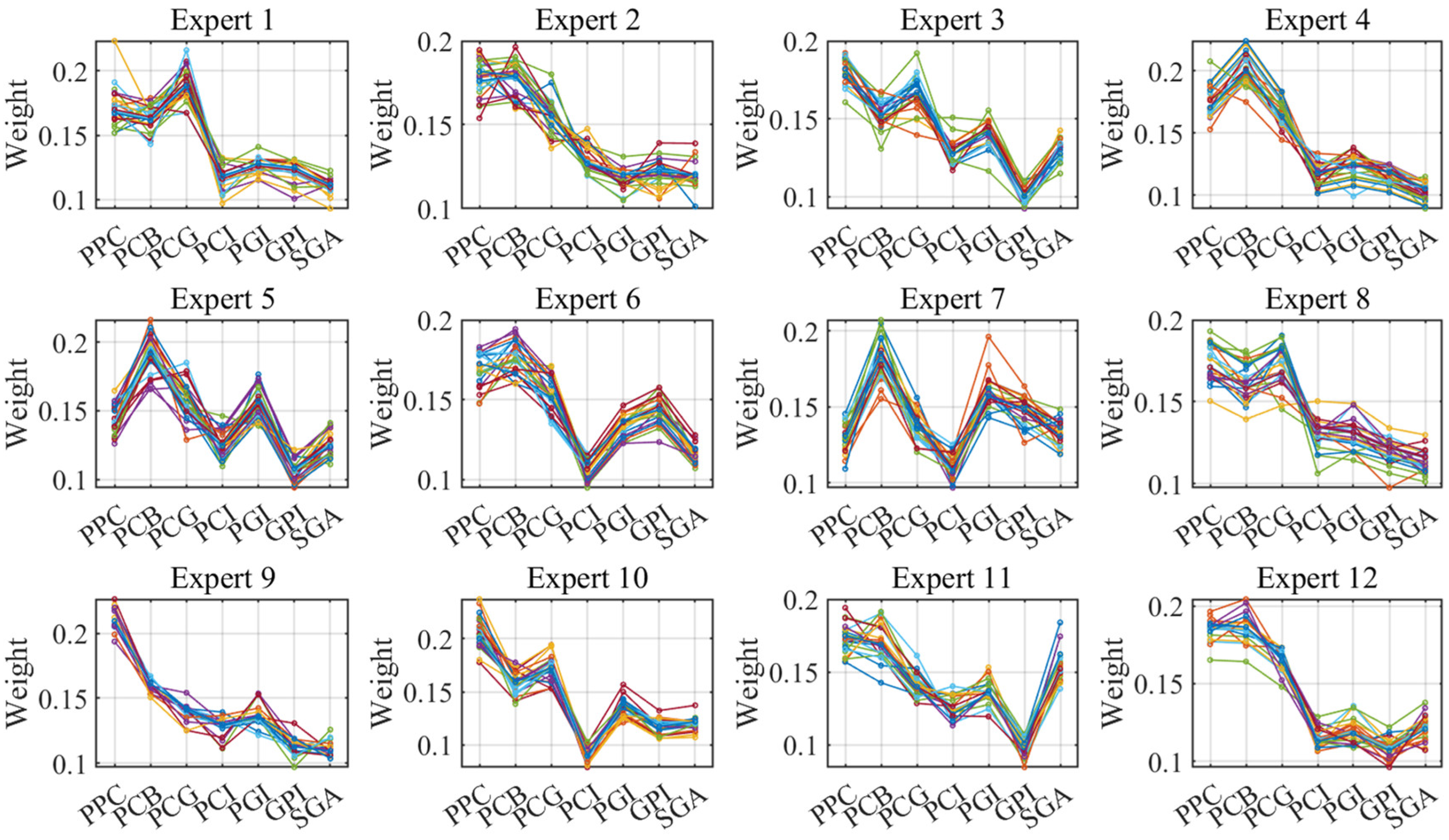
Figure 4 shows the weight preference distributions of the 13 experts for the second-level indicators across different bridges. In each subplot, different curves correspond to different bridges, and the horizontal axis represents the seven second-level indicators.

Figure 4. Weight preference distributions of different experts for second-level indicators across various bridges.

Differences in preferences are observed among experts. For experts 5, 6 and 10, the weight curves given for different bridges are relatively concentrated, indicating stable evaluation behavior across bridges. For experts 1, 2, 3 and 8, the curves are more dispersed, suggesting that evaluation preferences vary from bridge to bridge. This is attributed to the fact that experts often adjust the relative importance of indicators based on external factors such as the bridge’s environment and location, even though the structural forms of these HPBB are very similar.

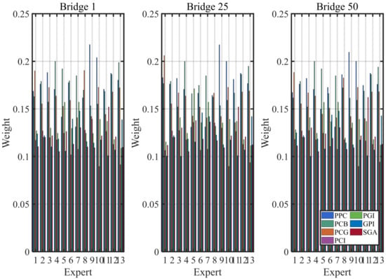
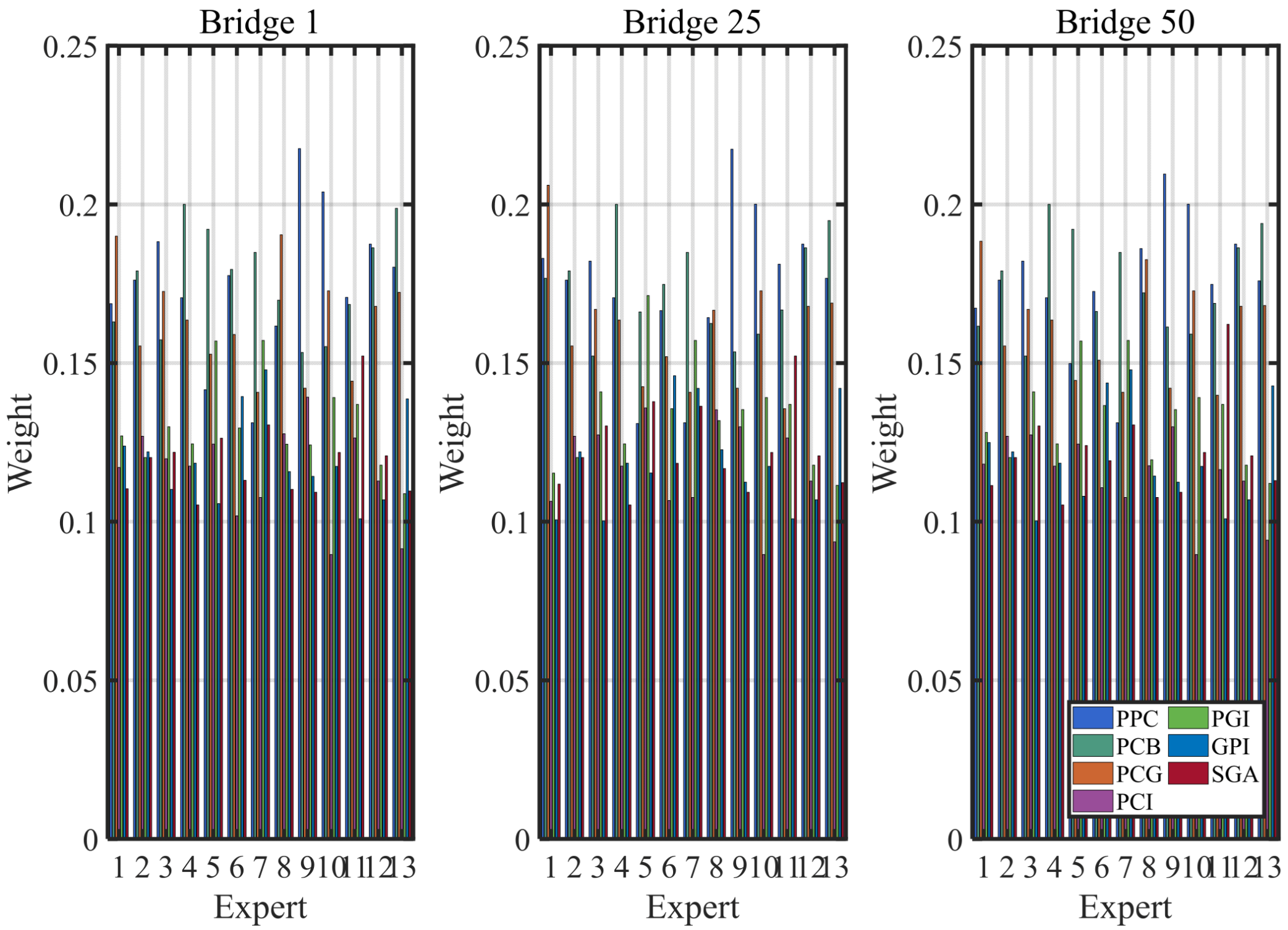
Three representative bridges (covering both the training and test sets) were further selected, and grouped bar charts (Figure 5) were used to compare the second-level weight allocations of all 13 experts for the same bridge. The results indicate that even for the same bridge, considerable disagreements in weight allocations across the second-level indicators are observed among different experts. This suggests that directly taking the arithmetic mean of multi-expert weights would be significantly affected by individual outlier judgments; therefore, a geometric median fusion strategy that is robust to outliers is necessary.

Figure 5. Comparison of second-level indicator weight distributions among different experts for the same bridge.

3.3.2. Expert Confidence Assessment

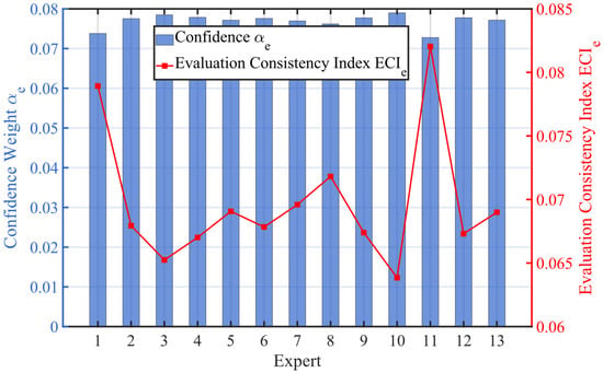
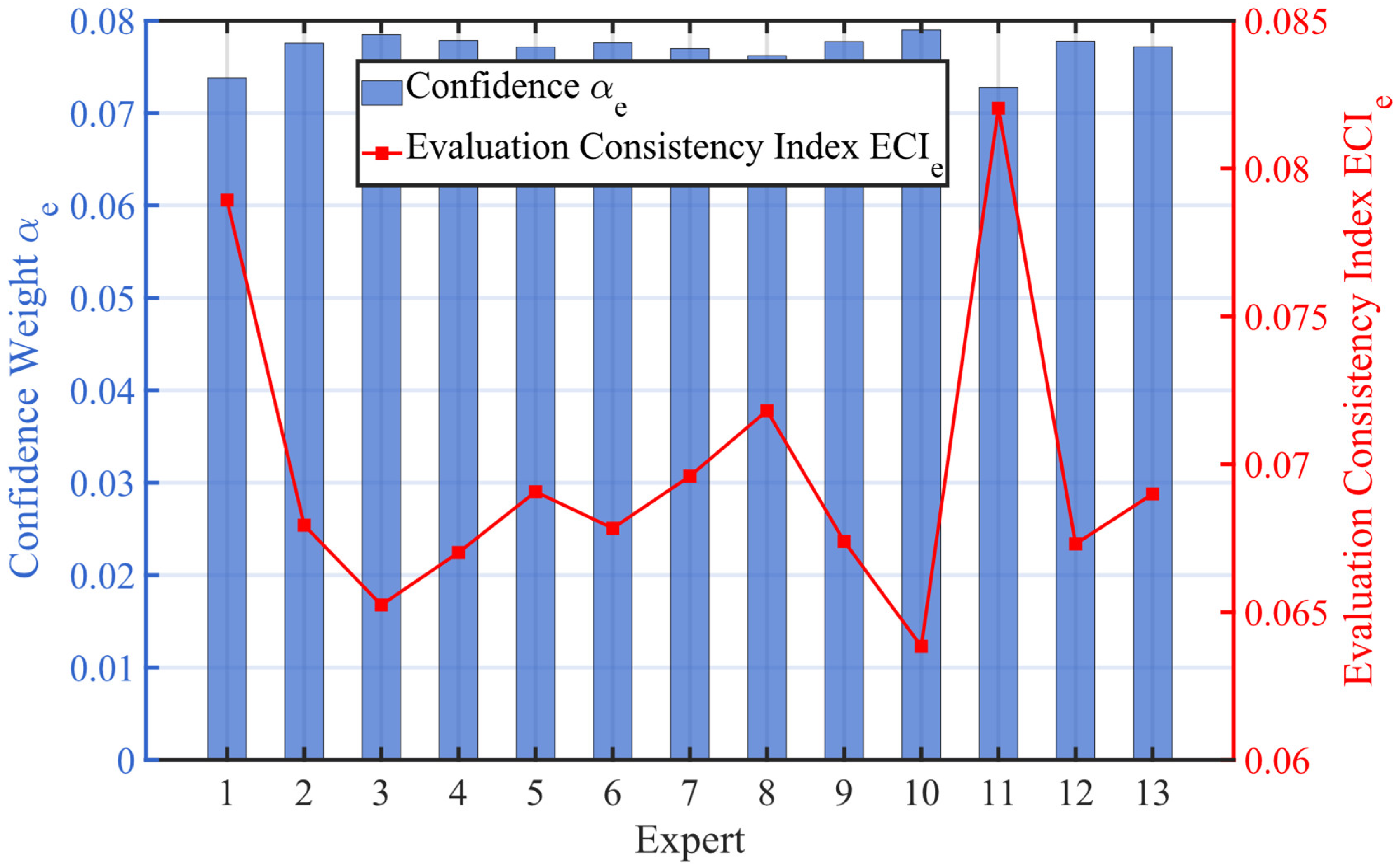
Following the ECI definition in Equation (26), an AMLP was trained separately on each expert’s training samples. The relative root-mean-square fitting error was used as the expert’s evaluation consistency index (ECI), quantifying how well a stable learned weight structure explains that expert’s scores. A smaller ECI indicates greater self-consistency. Figure 6 presents the ECI values (line, right axis) and confidence coefficients ${\alpha }_e$ (bars, left axis) for the 13 experts. ECI ranged from 0.064 to 0.082, while ${\alpha }_e$ ranged from 0.073 to 0.079; experts with more self-consistent ratings therefore re-ceived slightly greater influence in fusion.

Figure 6. Correspondence between each expert’s evaluation consistency index and confidence coefficient.

3.4. Manifold Redundancy Correction Analysis

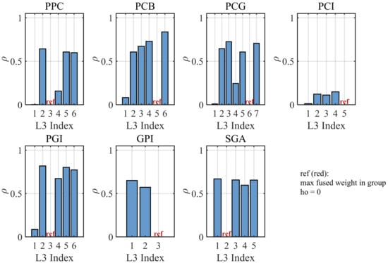
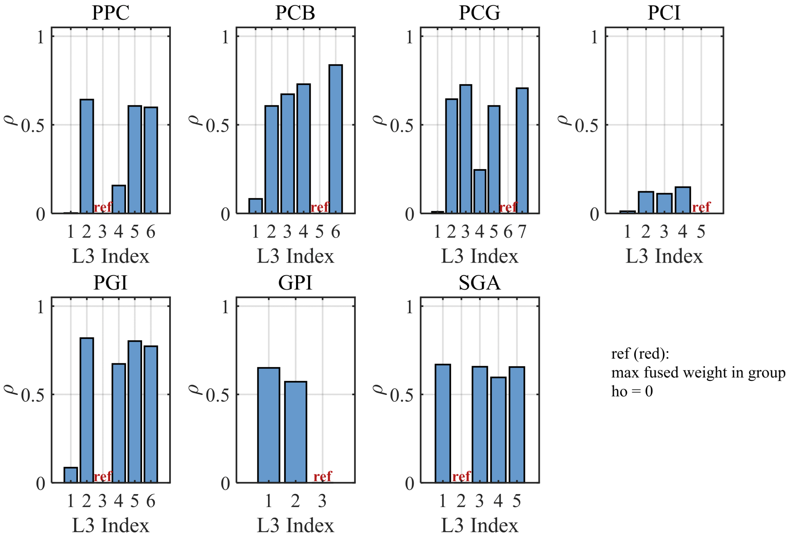
The manifold geodesic proximity ρ of third-level indicators relative to the reference indicator within each second-level group is presented in Figure 7. Significant differences were observed in the group means of ρ. The highest value was found in the PGI group (0.525), followed by the SGA group (0.516) and the PCG group (0.488), while the lowest value was found in the PCI group (only 0.079). This indicates that non-linear correlations exist among the third-level indicators within groups such as Precast Girder/Plate Installation and Span-by-Span Girder Assembly in the sample score space, whereas the indicators within the Pier and Column Installation group can be considered mutually independent.

Figure 7. Manifold geodesic proximity ρ of third-level indicators within each second-level group.

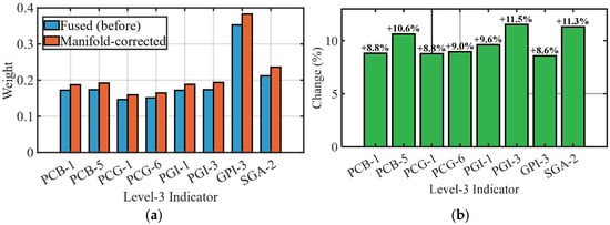
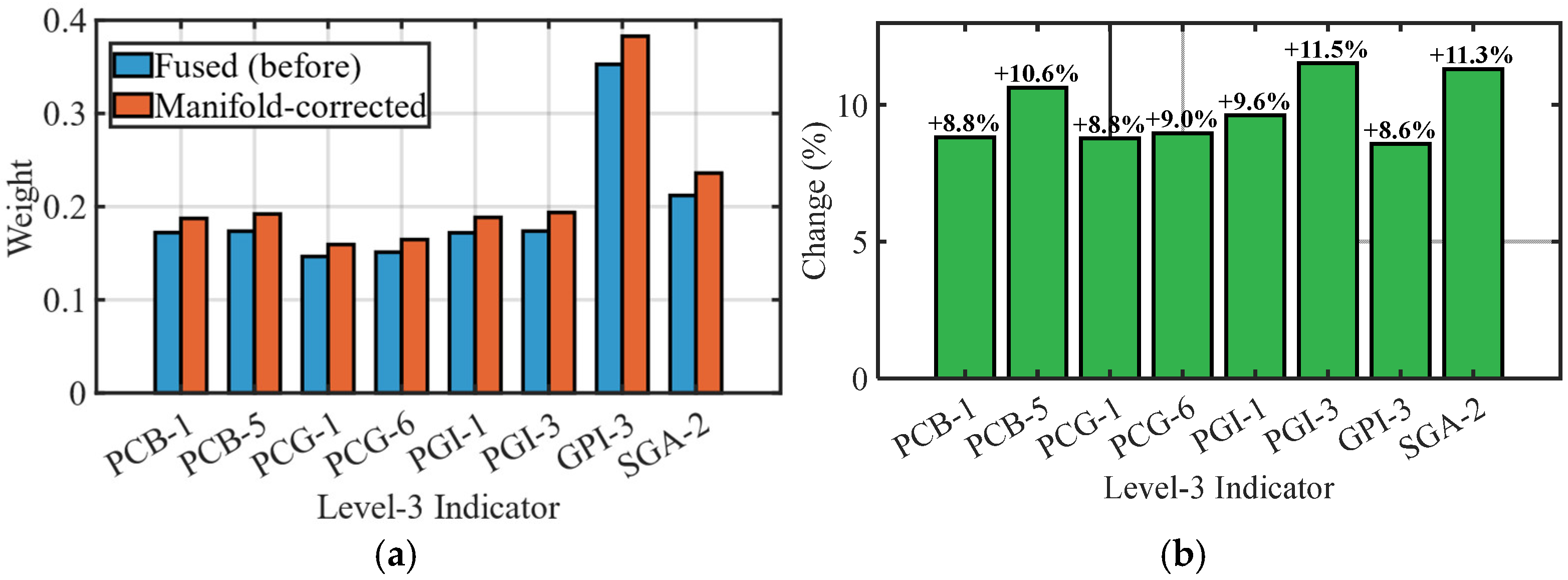
Figure 8a compares the weights before and after correction for the eight third-level indicators with the largest correction magnitudes, and Figure 8b presents their correction percentages (green indicating increases and red indicating decreases). The correction mechanism is as follows: indicators with higher proximity ρ to the reference indicator were attenuated more (δ = w* (1 − λρ)); the reference indicator itself, having ρ = 0, was not attenuated, and its weight increased relatively after intra-group normalization. Among all 38 third-level indicators, 24 were decreased and 14 were increased. The largest single increase was observed for the cross-sectional dimension in the PGI group (+11.5%, as the reference indicator of that group), and the largest decrease was observed for the embedded parts in the PCG group (−7.9%).

Figure 8. Manifold correction comparison of third-level indicator weights. (a) weights before and after correction for the eight indicators with the largest correction magnitudes; (b) correction percentages for the eight third-level indicators with the largest correction magnitudes.

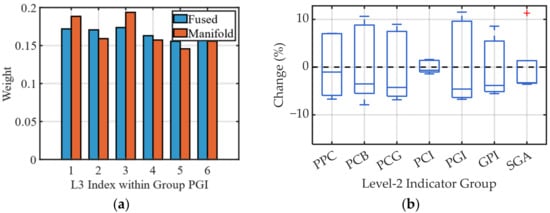
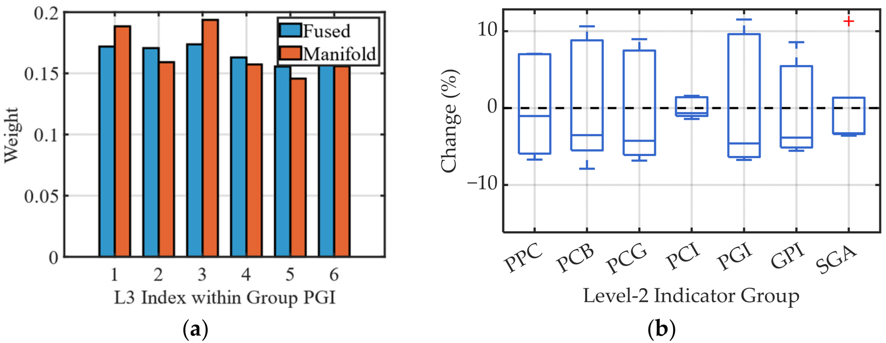
Figure 9a presents a detailed comparison of the weights of each third-level indicator within the PGI group, which had the largest correction magnitude, and Figure 9b presents the distribution of correction magnitudes across all seven second-level groups using box plots (red “+” indicating outliers). The medians of the correction magnitudes in all groups were observed to be within ±5%, and the correction magnitudes in the PCI group were concentrated within ±1.6%.

Figure 9. Analysis of manifold correction magnitude. (a) intra-group weight comparison for the group with the largest correction magnitude (PGI); (b) box plots of correction magnitude distributions for each second-level group.

3.5. Risk Incentive Function Analysis

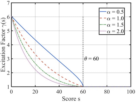
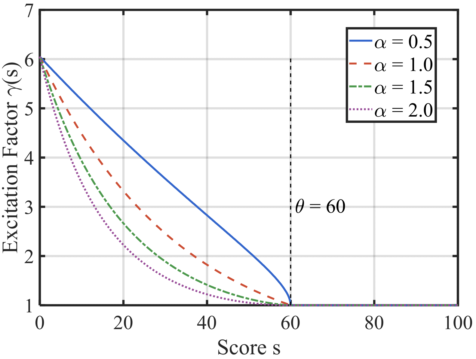
The qualified critical value used as the engineering lower bound of the risk trigger for risk incentive was set as θ_spec = 60. The safety threshold for each bottom-level indicator was determined as θ = max{θ_spec, μ − σ}, where μ and σ are the mean and standard deviation of the indicator scores estimated exclusively from the training bridges. The 90, 75, and 60 points values define the quality-grade boundaries, whereas the risk-sensitive module uses a single indicator-specific safety threshold defined by Equation (34); the 90 and 75 points boundaries are not additional risk-trigger thresholds in the present implementation. The response curves of the incentive function are plotted in Figure 10 for a fixed incentive intensity β = 1.8 and shape coefficients α = 0.5, 0.85, 1.2, and 2.0. When α = 1.0, the incentive factor grows approximately linearly as the score decreases below the threshold. When α < 1.0, the growth is steeper near the threshold, meaning that a slight exceedance triggers a relatively strong warning. When α > 1.0, the weight amplification only becomes significant at severely low scores. Considering that the finished product quality acceptance scenario requires high sensitivity to “critical near-failure” conditions, α was taken as 0.85, ensuring a sufficient response gradient near the threshold while reaching the upper limit of exp(β) = exp(1.8) ≈ 6.05 times weight amplification at score s = 0. All curves are continuous at s = θ with the incentive factor γ = 1, thereby ensuring function continuity. In the representative hold-out analysis, μ and σ were estimated from the 35 training bridges; in grouped cross-validation, they were re-estimated within each training fold and then frozen before application to the validation bridges.

Figure 10. Response curves of the incentive function under different shape coefficients (β = 1.8).

3.6. Analysis of the Weight Update Process

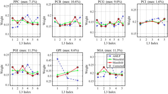
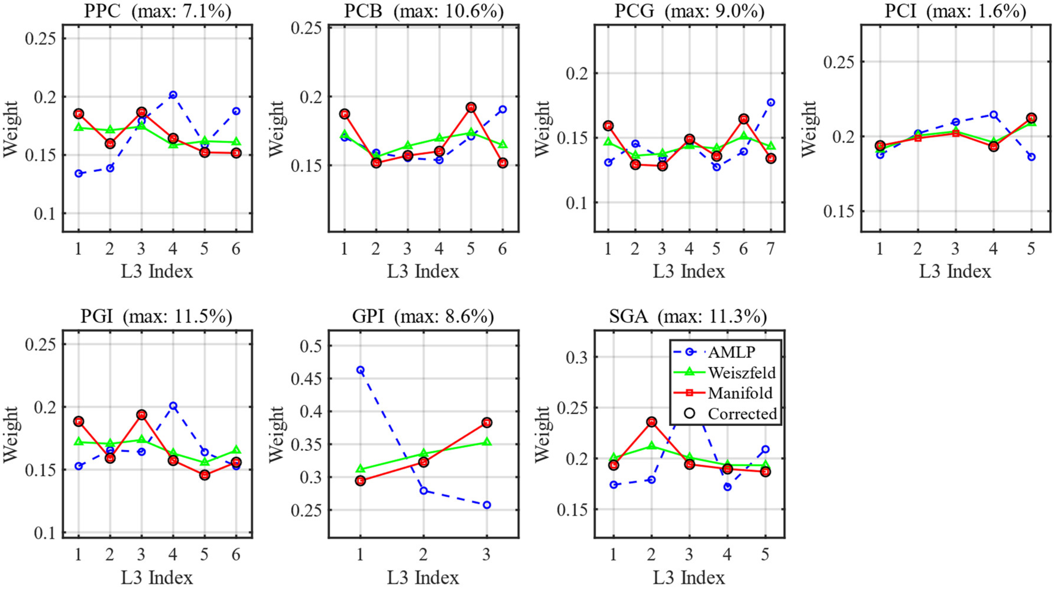
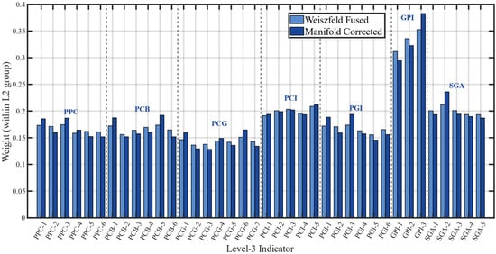
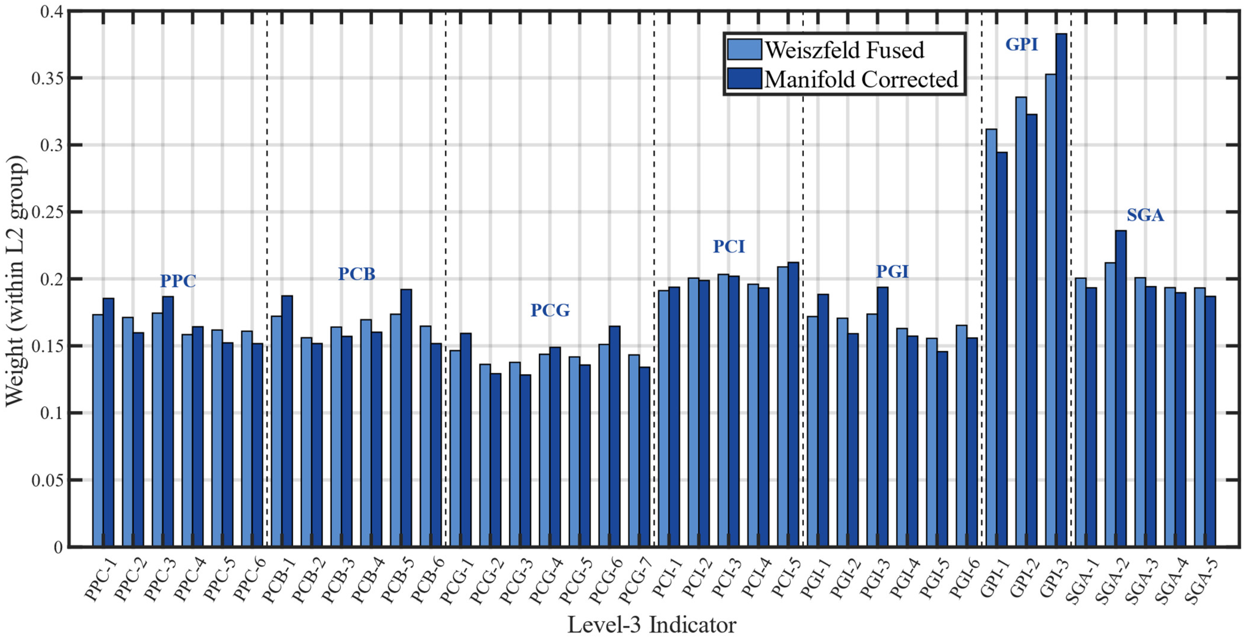
Taking third-level evaluation indicators as an example, each subplot in Figure 11 represents a second-level group. The blue dashed line, green line, and red line correspond to the attention-derived candidate initial coefficients, fused weights, and manifold-corrected weights, respectively. Black circles mark indicator points with corrections exceeding 0.002, and the maximum correction percentage for each group is annotated in the subplot title. A comparison of the weights of all 38 third-level indicators before and after manifold correction is presented in Figure 12 (separated by second-level group boundaries).

Figure 11. Three-stage evolution of third-level indicator weights within each second-level group.

Figure 12. Bar chart comparison of all third-level indicator weights before and after manifold correction (dashed lines indicate second-level group boundaries).

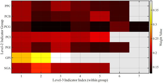
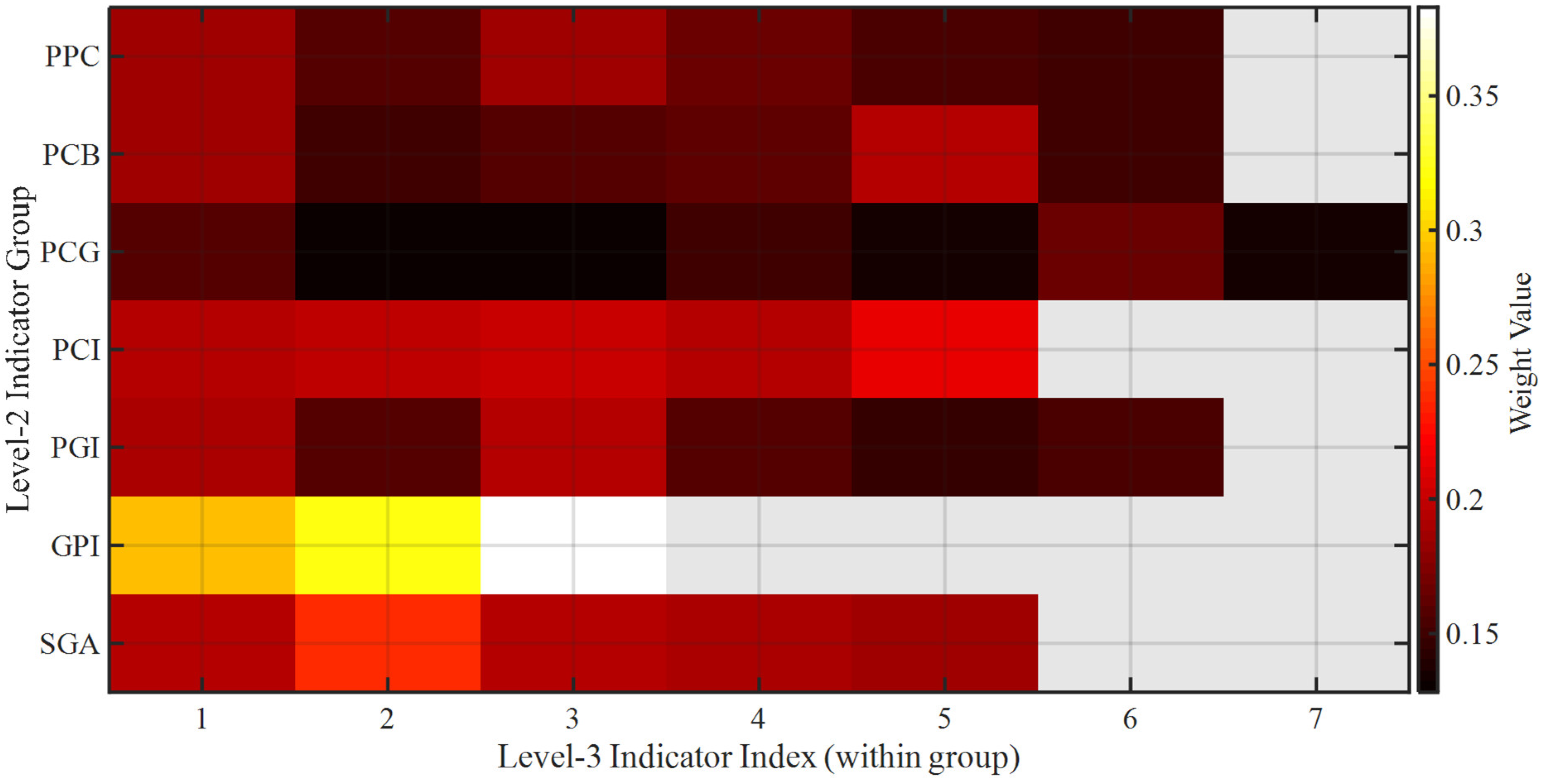
The final weight distribution of all third-level indicators after manifold correction is presented as a heatmap in Figure 13, where color intensity represents the magnitude of the weights. The final intra-group weights were generally located in the range of [0.128, 0.383]. Among them, the highest weight was observed for the “Adjacent Girder/Plate Top Elevation Difference” in the GPI group, and relatively balanced intra-group weight distributions were observed in six indicator groups, including PPC and PCB.

Figure 13. Heatmap of final third-level indicator weights.

3.7. Model Accuracy Assessment

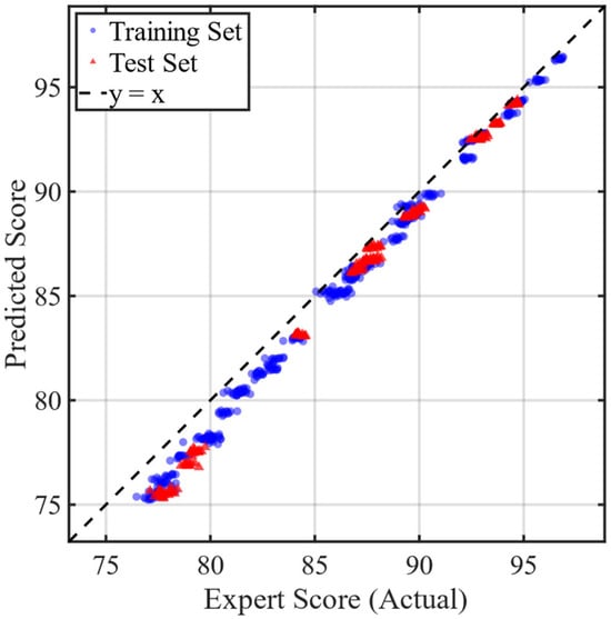
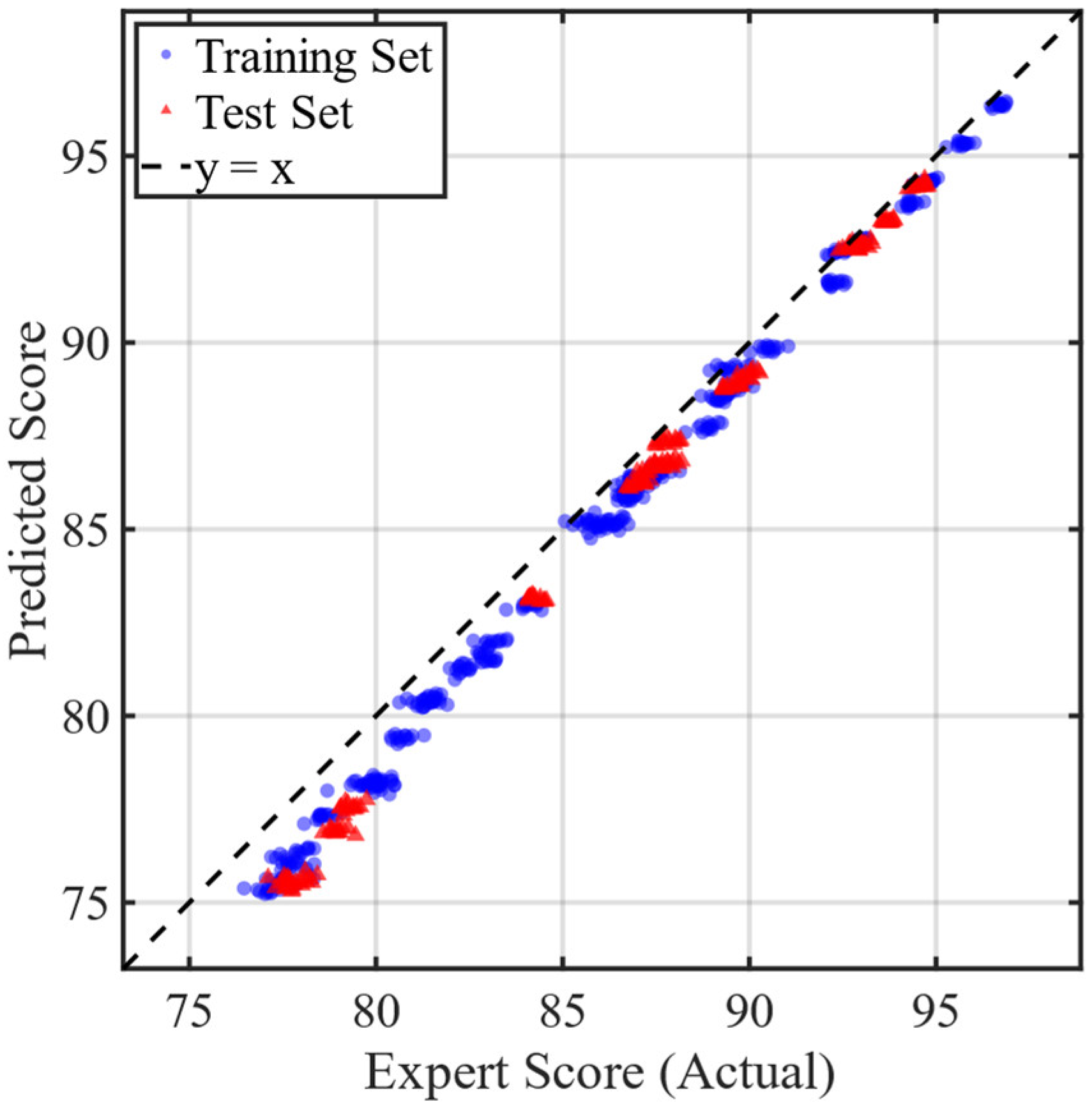
Figure 14 presents the scatter plot of predicted versus true values on the training and test sets. Five-fold bridge-level grouped cross-validation was conducted using one prespecified bridge partition. The proposed method achieved a mean fold-level MAE of 1.0668 ± 0.1023 and a mean fold-level RMSE of 1.2180 ± 0.0802. Pooling the out-of-fold predictions from the five folds yielded RMSE = 1.2201, R² = 0.9536, and MRE = 1.2845%. The 1.2180 ± 0.0802 value describes variation among the five fold-specific RMSE values, whereas 1.2201 is the RMSE calculated once from all pooled out-of-fold predictions.

Figure 14. Scatter plot of predicted versus true values on training and test sets.

It is worth noting that the distribution of scatter points exhibited regular differences related to the score intervals. In the low-score range (e.g., below 80), some predicted values were observed to be systematically higher than the true values, meaning that the scatter points were generally located above the diagonal. In the high-score range (e.g., above 90), the deviations between predicted and true values were found to narrow considerably, and the scatter points were more closely concentrated around the diagonal. This observation suggests that the fitting accuracy of the model was higher in the high-score segment than in the low-score segment, and that a certain degree of overestimation existed in the predictions for low-score samples.

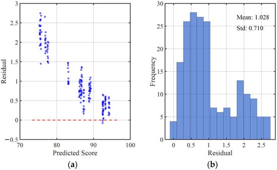
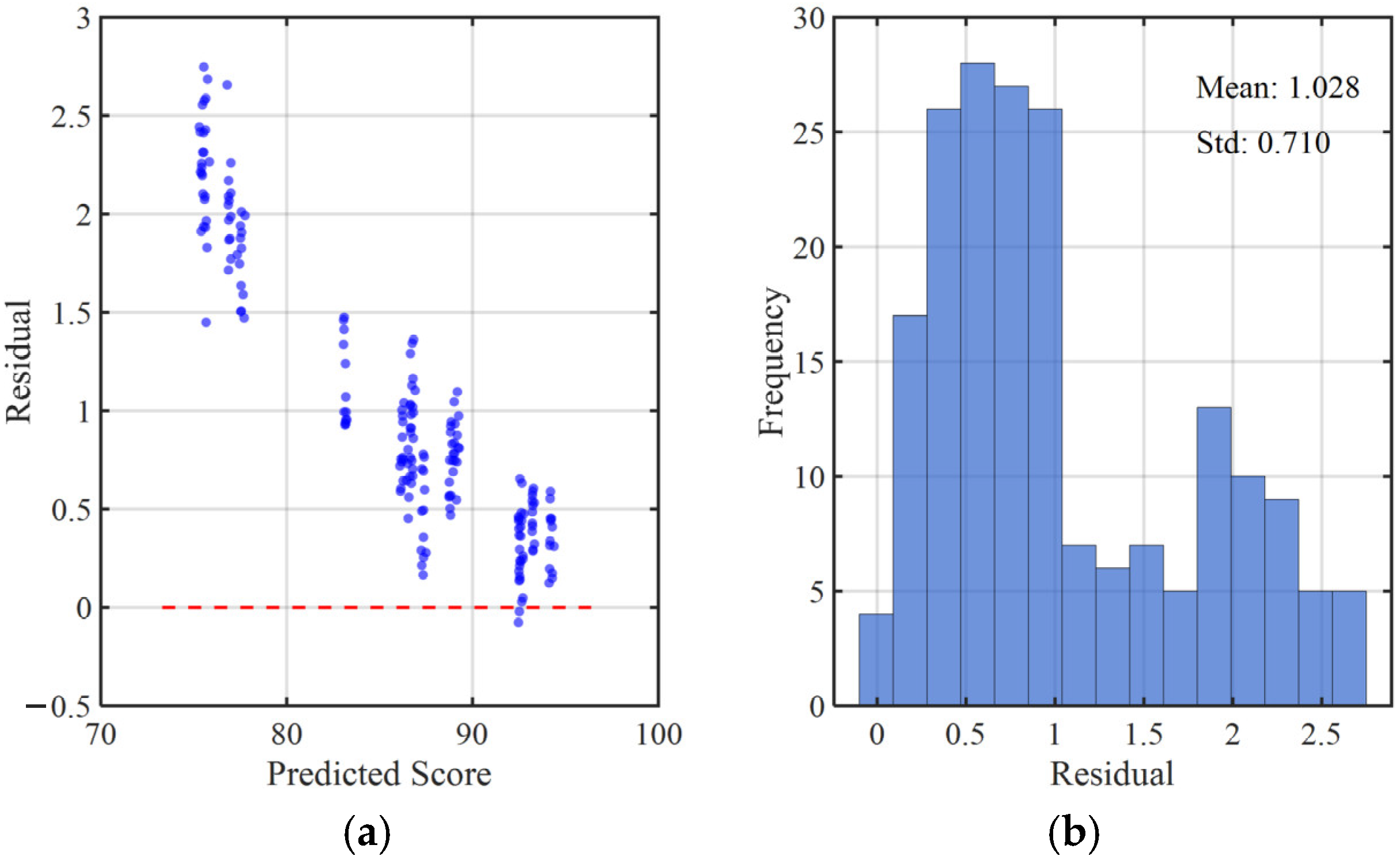
Further analysis of the residuals on the test set was conducted (Figure 15). Figure 15a presents the scatter distribution of residuals against predicted values. When the predicted scores were in the interval [90, 100], the residuals were concentrated near zero with the smallest dispersion. As the predicted scores decreased, the range of residual fluctuation was observed to expand, and a more pronounced positive shift in residuals was found in the low-score interval, which is consistent with the observations from the scatter plot. Figure 15b shows the histogram of residual distribution, which is predominantly positive, with a mean of 1.024 and a standard deviation of 0.706. This indicates an average overestimation of approximately 1.02 points (1.02% of the 100-point scale) on the test records; the magnitude remains small relative to the full scoring range, but the positive residual bias is reported explicitly rather than interpreted as negligible.

Figure 15. Residual results on the test set. (a) scatter plot of residuals on the test set; (b) histogram of residual distribution.

The evaluation metrics on both the training and test sets are summarized in Table 5. The test set MAE was 1.025 and RMSE was 1.243, which are very close to the training set values (MAE = 0.991, RMSE = 1.131), with differences not exceeding 5%. This suggests that no significant overfitting occurred.

Table 5. Summary of model evaluation metrics.

Dataset	MAE	RMSE	R2	MRE (%)
Training set	0.991	1.131	0.960	1.19
Test set	1.025	1.243	0.953	1.24

3.8. Module Validation via Ablation and Sensitivity Analysis

Table 6 summarizes the complete 2³ factorial ablation results. For each of five inde-pendent repetitions, predictions from the five validation folds were pooled before cal-culating bridge-level metrics; the table reports the mean and between-repetition standard deviation over the five repetitions.

Table 6. Full-factorial ablation results.

GM	Iso	Risk	MAE	RMSE	R2
×	×	×	1.2065 ± 0.0104	1.3684 ± 0.0130	0.9417 ± 0.0011
√	×	×	0.9894 ± 0.0059	1.0699 ± 0.0080	0.9643 ± 0.0005
×	√	×	0.9552 ± 0.0092	1.0306 ± 0.0102	0.9730 ± 0.0006
√	√	×	0.9729 ± 0.0118	1.0284 ± 0.0131	0.9731 ± 0.0008
×	×	√	1.2037 ± 0.0074	1.3653 ± 0.0104	0.9419 ± 0.0009
√	×	√	0.9921 ± 0.0089	1.0729 ± 0.0107	0.9641 ± 0.0007
×	√	√	1.0724 ± 0.0103	1.2296 ± 0.0114	0.9529 ± 0.0009
√	√	√	1.0702 ± 0.0121	1.2271 ± 0.0141	0.9531 ± 0.0011

The full-factorial ablation results demonstrate that the three modules serve different purposes. Isomap alone produced the lowest MAE of 0.9552 ± 0.0092, while the combination of geometric-median fusion and Isomap achieved the lowest RMSE of 1.0284 ± 0.0131 and the highest R² of 0.9731 ± 0.0008. Relative to the baseline configuration, the RMSE reductions of the GM-only and Isomap-only configurations were 21.8% and 24.7%, respectively.

The additional RMSE improvement obtained by adding GM to Isomap was only 0.0022, indicating functional overlap between the two modules in suppressing unstable or redundant weights. In contrast, adding the risk-sensitive module to the GM-Isomap configuration increased RMSE from 1.0284 to 1.2271. Nevertheless, the complete model still retained a 10.3% RMSE improvement relative to the baseline configuration.

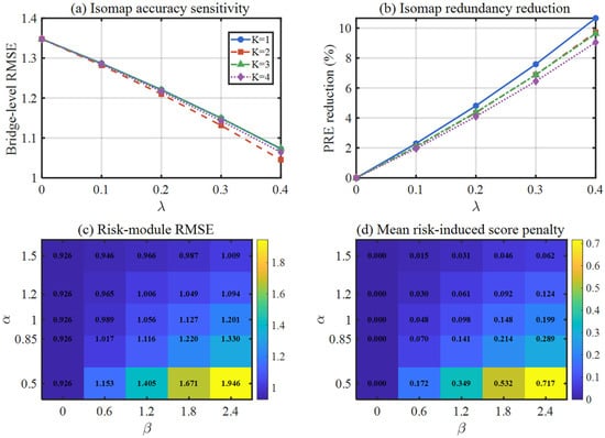
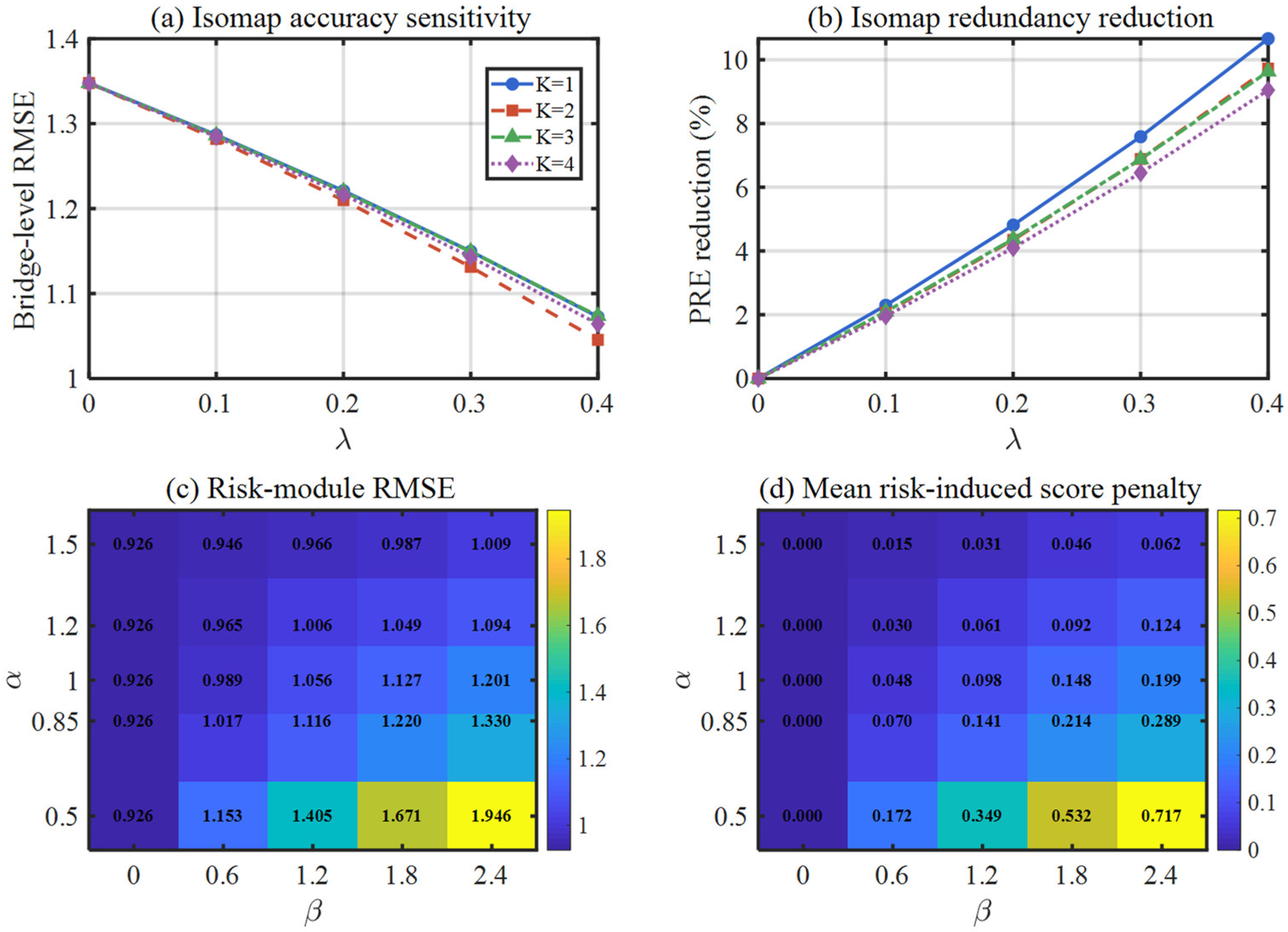
A fixed bridge-level five-fold partition was used to examine local robustness around the prespecified settings. PRE denotes proximity-weighted redundancy exposure, and PRI denotes the pairwise geodesic-kernel redundancy index; lower values indicate less weight concentration on geodesically similar indicators. Figure 16a,b shows nearly overlapping curves for K = 1–4, indicating limited sensitivity to the neighbor number. Increasing λ strengthened redundancy correction, reduced pooled out-of-fold RMSE, and increased PRE reduction. At K = 3 and λ = 0.20, the pooled RMSE was 1.2201, while PRE and PRI were reduced by 4.38% and 1.84%, respectively. Figure 16c,d shows that increasing β or decreasing α increases both the risk-induced score penalty and RMSE, revealing a controllable trade-off between risk sensitivity and agreement with average expert ratings. At α = 0.85 and β = 1.80, the mean penalty was 0.2144 points overall and 0.3285 points for bridges containing below-threshold indicators, with a deficit–penalty correlation of 0.9169. In the controlled counterfactual mechanism di-agnostic, risk adjustment produced an additional mean score drop of 0.3732 points and a mean amplification ratio of 1.45. No natural sample changed grade; thus, the default setting refined continuous scores without altering the observed grade conclusions. This result also reflects a limitation of the present dataset: naturally occurring near-threshold or severely low-score bridges were limited, so the risk-sensitive module improves responsiveness to low-score indicators but its grade-changing benefit cannot yet be demonstrated from natural samples under the default setting. Future validation should therefore include more bridges with borderline and locally deficient indicators, with predictive accuracy and risk sensitivity reported jointly.

Figure 16. Parameter sensitivity of the Isomap and risk-sensitive modules: (a) RMSE under different K and λ; (b) PRE and PRI reductions; (c) RMSE under different α and β; (d) mean score penalty induced by risk adjustment.

3.9. Comparison of Evaluation Methods

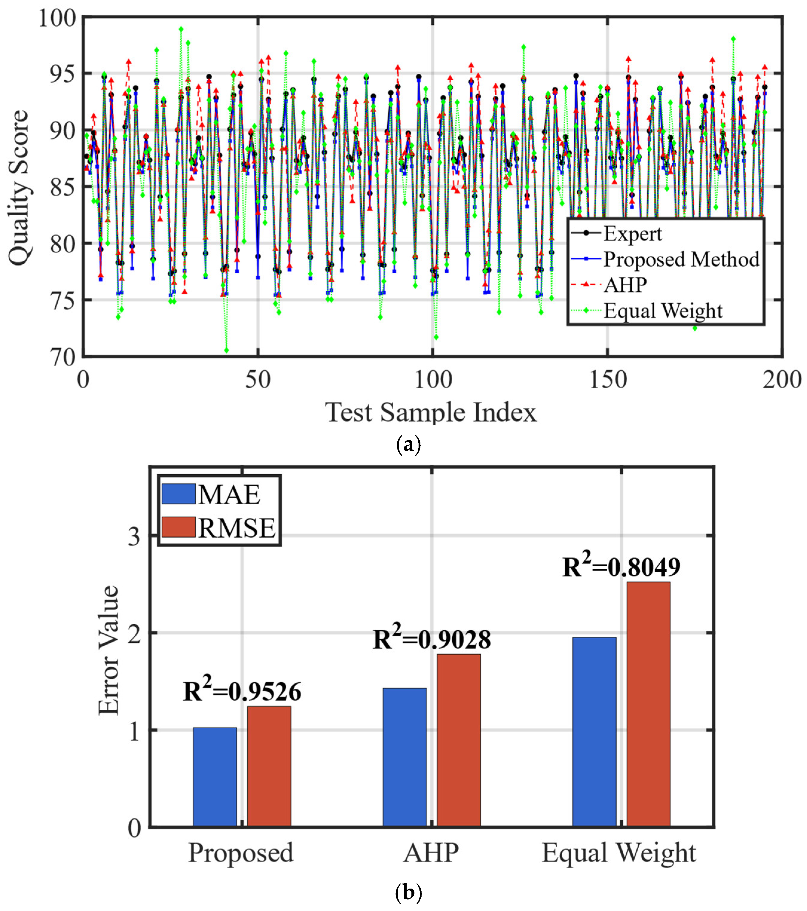
To quantitatively assess the performance advantages of the proposed method over existing methods, the proposed method was compared with the traditional AHP method and the equal-weight method on the test set.

The comparative experimental settings were as follows. For the traditional AHP method, the arithmetic mean of all expert weights was directly taken as the indicator weights, without manifold correction or risk incentive, and the comprehensive score was calculated by weighted summation. For the equal-weight method, equal weights were assigned to indicators at all levels, without distinguishing differences in indicator importance. All three methods used the same continuous indicator-score transformation, the same 15 held-out test bridges, and the same bridge-level reference score defined as the mean of the 13 expert comprehensive ratings; only the indicator-weight determination and subsequent weight-adjustment procedures differed among methods.

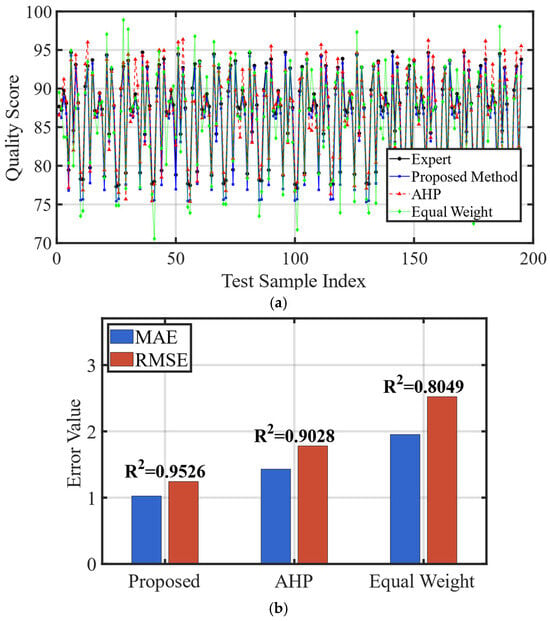
The comparison curves of predicted scores and true expert scores for the three methods on each test sample are shown in Figure 17a. The prediction curve of the proposed method exhibited the highest agreement with the true values, with small deviations at all sample points. The traditional AHP method showed noticeable deviations on some samples, and the largest deviations were observed for the equal-weight method.

Figure 17. Comparison of three evaluation methods. (a) score comparison curves on test samples; (b) MAE and RMSE comparison.

Compared with the traditional AHP method and the equal-weight method, the MAE of the proposed method was reduced by 28% and 47%, respectively, and the RMSE was reduced by 30% and 50%, respectively. The R² was improved by approximately 0.05 and 0.18, respectively (Figure 17b). The model parameters for each method are summarized in Table 7.

Table 7. Comparison of evaluation metrics on the test set for three methods.

Method	MAE	RMSE	R2
Proposed method	1.02	1.24	0.953
Traditional AHP	1.44	1.79	0.903
Equal-weight method	1.95	2.52	0.805

4. Conclusions

To address the shortcomings of existing intelligent quality evaluation methods for the finished products of Highway Prefabricated Beam Bridges (HPBB), a graded evaluation method for construction quality based on manifold learning and probability distributions is proposed in this paper. Following the construction process of HPBB, a four-level evaluation index system was constructed, centered on prefabricated component quality and installation quality. An indicator score transformation method based on the two-point distribution and the two-sided cumulative probability of the normal distribution was proposed, by which the original measurement data were directly mapped to continuous scores. The specific mathematical mapping relationship between measured results and evaluation indices was thereby preserved, effectively solving the industry-wide problem of highly concentrated evaluation results above the qualified level with severely insufficient discrimination, and enabling refined grading of bridge construction quality.

The Softmax output of the AMLP is used as an attention-derived candidate initial importance vector rather than as an exact indicator-contribution vector. Whole-network Integrated Gradients analysis shows a mean expert-wise Spearman correlation of 0.7490 ± 0.0681 and a mean Top-10 overlap of 6.92/10, indicating a broadly consistent global importance ordering after the downstream fully connected layers are taken into account. Furthermore, the initialization sensitivity analysis shows that under bounded multiplicative perturbations ranging from ±5% to ±20%, the test RMSE and MAE vary only slightly relative to the baseline (e.g., RMSE of 1.2838 vs. 1.2479 at ±20% perturbation), with a maximum prediction mean absolute difference of only 0.0607 points, and the final-weight Spearman correlation with the unperturbed model remains above 0.72. This sensitivity analysis suggests that the subsequent fusion and correction procedures are not sensitive to uncertainty in the candidate initialization.

The intrinsic geometric dependencies among indicators were quantified through Isomap-based manifold correction, eliminating the bias caused by double-counting of the same quality dimension in traditional methods. Correction magnitudes ranged from 1.6% to 11.5%, and a positive correlation was observed between group-wise manifold proximity and correction magnitude. The arithmetic mean of traditional AHP was replaced by the Weiszfeld geometric median fusion framework, which reduced the distortion effect of outlier expert extreme preferences on consensus weights. The robustness of the fusion results was further ensured through the incorporation of a confidence weighting mechanism. The threshold-triggered risk-sensitive weight incentive mechanism addressed the inherent defect in the traditional linear weighted summation framework—namely, the dilution of low scores of critical indicators by high scores of other indicators—through nonlinear amplification via an exponential incentive function, thereby enabling timely identification and early warning of major quality and safety hazards. Because no natural sample changed grade under the default risk-sensitive setting, the present evidence supports enhanced low-score sensitivity at the continuous-score level, while grade-level benefits require further validation on datasets containing more borderline or locally deficient bridges.

The full-factorial ablation further revealed the functional division among the three modules. Isomap correction and geometric-median fusion primarily serve predictive accuracy—enabling Isomap alone reduced RMSE by 24.7%, and the combination of GM and Isomap achieved the lowest RMSE of 1.0284 and the highest R² of 0.9731. The risk-sensitive module, by design, trades a degree of overall accuracy for enhanced sensitivity to local critical defects, increasing RMSE from 1.0284 to 1.2271 when incorporated into the complete model, yet still retaining a 10.3% improvement over the baseline. Parameter sensitivity analysis showed that the Isomap module is insensitive to the neighbor number K (RMSE variation among K = 1–4 was only about 1.3%), with λ serving as the main control parameter: at the default K = 3 and λ = 0.20, RMSE was 1.2201, with PRE and PRI reduced by 4.38% and 1.84%, respectively, and the PRE reduction increased monotonically with λ to 9–11%. For the risk module, β = 0 deactivated the module (RMSE = 0.926, zero penalty), while increasing β to 2.40 raised RMSE to 1.330 and the penalty to 0.289 points, demonstrating a monotonic and controllable response; at the default α = 0.85 and β = 1.80, the deficit–penalty correlation was 0.9169, and the counterfactual diagnostic showed an additional score drop of 0.3732 points with an amplification ratio of 1.45. Taken together, the default parameters lie within a stable response region with directionally consistent parameter effects.

The proposed method achieved an MAE of 1.025 and an RMSE of 1.243 on the test set. Five-fold grouped cross-validation at the bridge level further showed that the proposed method achieved an RMSE of 1.2180 ± 0.0802, with an overall R² of 0.9536. The limited variation across folds indicates that the model performance remains stable across different bridge subsets. Compared with the traditional AHP method and the equal-weight method, the RMSE was reduced by 30% and 50%, respectively. This provides a digitally integrable intelligent decision-support tool for the safety control of prefabricated bridges. The proposed method can directly read the raw measurement data of all indicators from the database, dynamically compute the indicator scores and fused weights, and thus perform real-time monitoring and early warning of construction quality for prefabricated beam bridges. The method is practically operable: it only requires connection to an existing quality-inspection database and configuration of the corresponding parameters. Future research will further explore the integrated application of this framework with digital twins and BIM platforms, so as to enable real-time perception and dynamic early warning of quality status during the construction process.

References

- Li, C.; Zeng, K.; Zhang, T.; Tang, X.; Xu, N. Monitoring–Modeling Integrated Assessment of Temperature-Induced Prestress Variations in Prestressed Concrete Beams During Construction. Buildings 2026, 16, 1095. [Google Scholar] [CrossRef] [Scilit]
- Furkan, M.O.; Mao, Q.; Livadiotis, S.; Mazzotti, M.; Aktan, A.E.; Sumitro, S.P.; Bartoli, I. Towards rapid and robust measurements of highway structures deformation using a wireless sensing system derived from wired sensors. J. Civ. Struct. Health Monit. 2020, 10, 297–311. [Google Scholar] [CrossRef] [Scilit]
- Furkan, M.O.; Mao, Q.; Livadiotis, S.; Mazzotti, M.; Aktan, A.E.; Sumitro, S.P.; Bartoli, I. Research on Influencing Factors and Accident-Causing Mechanisms of Railway Cable-Stayed Bridge Construction Safety Based on Fuzzy DEMATEL-ISM. Buildings 2026, 16, 2077. [Google Scholar] [CrossRef] [Scilit]
- Oliveira, J.G.; de França Moura, J.M.; dos SMota, V.; do Nascimento Filho, S.I.; Gaspar, C.M.; Sotelino, E.D.; Carrazedo, R. Dynamic testing and finite element model updating for a viaduct structural assessment. J. Civ. Struct. Health Monit. 2025, 15, 2279–2297. [Google Scholar] [CrossRef] [Scilit]
- Bai, H.; Zhang, Y.; You, B.; Chen, K. Comprehensive Design Optimization Framework for Prestressed Concrete Continuous Beam Bridge Using Genetic Algorithm and Backpropagation Neural Network. Buildings 2025, 15, 1344. [Google Scholar] [CrossRef] [Scilit]
- Lv, G.; Chen, L.; Wang, P.; Wang, Q.; Li, J.; Zhang, J.; Mebarki, A.; Dou, Z. Interval prediction of bridge expansion joint evolution: Based on complex network analysis and fuzzy information granulation. J. Civ. Struct. Health Monit. 2025, 15, 2705–2724. [Google Scholar] [CrossRef] [Scilit]
- Zhou, D.; Zhou, Y.; Zhang, X.; Xu, K. Surface Quality Evaluation of Heavy and Medium Plate Using an Analytic Hierarchy Process Based on Defects Online Detection. ISIJ Int. 2022, 62, 1461–1468. [Google Scholar] [CrossRef] [Scilit]
- Darban, S.; Tehrani, H.G.; Karballaeezadeh, N.; Mosavi, A. Application of analytical hierarchy process for structural health monitoring and prioritizing concrete bridges in Iran. Appl. Sci. 2021, 11, 8060. [Google Scholar] [CrossRef] [Scilit]
- Ishizaka, A.; Labib, A. Review of the main developments in the analytic hierarchy process. Expert Syst. Appl. 2011, 38, 14336–14345. [Google Scholar] [CrossRef] [Scilit]
- Jin, R.; Wang, L.; Zhang, T.; Li, Q. Bridge Construction Quality Evaluation Based on Combination Weighting Method-Technique for Order Preference by Similarity to an Ideal Solution Theory. Appl. Sci. 2023, 13, 12018. [Google Scholar] [CrossRef] [Scilit]
- Shu, J.; Ma, H.; Ding, W. Improved Evidence Fusion Theory for the Safety Assessment of Prestressed Concrete Bridges. Buildings 2024, 14, 1144. [Google Scholar] [CrossRef] [Scilit]
- Wen, X.L.; Lei, W.; Dan, D.H. Study on a measurement index of transverse collaborative working performance of prefabricated girder bridges. Adv. Struct. Eng. 2017, 20, 1879–1890. [Google Scholar] [CrossRef] [Scilit]
- Zhu, Z.; Ye, K.; Yu, X. State-Based Technical Condition Assessment and Prediction of Concrete Box Girder Bridges. Buildings 2024, 14, 543. [Google Scholar] [CrossRef] [Scilit]
- Matos, J.; Fernandes, S.; Tran, M.Q. Developing a comprehensive quality control framework for roadway bridge management: A case study approach using key performance indicators. Appl. Sci. 2023, 13, 7985. [Google Scholar] [CrossRef] [Scilit]
- Luo, H.; Xu, C.; Gan, X.; Liu, M.; Guo, X.; Guo, H. The train-bridge coupled vibration analysis of a long-span prestressed concrete continuous beam bridge under creep deformation effect. Appl. Sci. 2022, 12, 11838. [Google Scholar] [CrossRef] [Scilit]
- Liu, K.; Zhang, L. Prediction of bridge component conditions using convolutional neural networks. Front. Built Environ. 2020, 6, 88. [Google Scholar]
- Shen, C.; Jiang, B.; Yue, L. LSTM combined with BIM technology in the management of small and medium-sized span highway concrete beam bridges. Results Eng. 2023, 20, 101539. [Google Scholar] [CrossRef] [Scilit]
- Concepcion, R.S.; Ilagan, L.C. Application of hybrid soft computing for classification of reinforced concrete bridge structural health based on thermal-vibration intelligent system parameters. In Proceedings of the 2019 IEEE 15th International Colloquium on Signal Processing & Its Applications (CSPA); IEEE: Piscataway, NJ, USA, 2019; pp. 207–212. [Google Scholar]
- Alsharqawi, M.; Zayed, T.; Abu Dabous, S. Integrated condition-based rating model for sustainable bridge management. J. Perform. Constr. Facil. 2020, 34, 04020091. [Google Scholar] [CrossRef] [Scilit]
- Malekly, H.; Mousavi, S.M.; Hashemi, H. A fuzzy integrated methodology for evaluating conceptual bridge design. Expert Syst. Appl. 2010, 37, 4910–4920. [Google Scholar] [CrossRef] [Scilit]
- Jiang, C.; Xiong, W.; Wang, Z.; Cai, C.; Yang, J. Transverse connectivity and durability evaluation of hollow slab bridges using surface damage and neural networks: Field test investigation. Appl. Sci. 2023, 13, 4851. [Google Scholar] [CrossRef] [Scilit]
- Xia, Y.; Lei, X.; Wang, P.; Sun, L. Artificial intelligence based structural assessment for regional short-and medium-span concrete beam bridges with inspection information. Remote Sens. 2021, 13, 3687. [Google Scholar] [CrossRef] [Scilit]
Disclaimer/Publisher’s Note: The statements, opinions and data contained in all publications are solely those of the individual author(s) and contributor(s) and not of MDPI and/or the editor(s). MDPI and/or the editor(s) disclaim responsibility for any injury to people or property resulting from any ideas, methods, instructions or products referred to in the content. |
© 2026 by the authors. Licensee MDPI, Basel, Switzerland. This article is an open access article distributed under the terms and conditions of the Creative Commons Attribution (CC BY) license.