Cost Prediction of Residential Buildings Based on an Improved SSA-BP Neural Network

Abstract

To enhance the accuracy, stability, and interpretability of residential building cost prediction models, and thereby provide a reliable basis for project investment decision-making. This study takes Sichuan Province as the research area and develops an improved sparrow search algorithm (ISSA). The performance of the Genetic Algorithm (GA), Wolf Pack Algorithm (WPA), Sparrow Search Algorithm (SSA), and ISSA was first evaluated and compared using benchmark test functions. Subsequently, nine prediction models, including Back Propagation Neural Network (BP), GA-BP, WPA-BP, SSA-BP, ISSA-BP, Random Forest (RF), ISSA-RF, Extreme Gradient Boosting (XGBoost), and ISSA-XGBoost, were established for comparative analysis. Finally, SHapley Additive exPlanations (SHAP) were employed to rank the key factors affecting construction cost. The results show that: (1) The ISSA algorithm demonstrates excellent convergence accuracy, stability and speed on benchmark test functions. (2) The ISSA-BP model achieved an average coefficient of determination (R²) of 0.9773, an average root mean square error (RMSE) of 39.2339, an average mean absolute error (MAE) of 17.0973, an average mean absolute percentage error (MAPE) of 0.6293, and an average mean bias error (MBE) of 9.1583. Compared with the other models, ISSA-BP exhibited the best overall predictive performance. (3) SHAP analysis indicates that indicators such as total building area and structure type have the greatest impact on project cost, while roof form and roof waterproofing have the least influence. This study can serve as a reference for refining and intelligently managing construction project costs.

1. Introduction

As a key industry for the national economy, construction plays an essential role in promoting urbanization, safeguarding employment and sustaining stable economic growth [1]. However, the growing scale and complexity of construction projects have intensified market competition, posing significant challenges to cost management [2]. In this context, accurate cost estimation is essential for effective cost control and critical to project success [3]. Inaccurate cost estimation can result in budget overruns, delays and suboptimal project outcomes [4,5]. Therefore, to reduce errors in estimation caused by a lack of systematic approaches, much of the research in this area has focused on overcoming inaccurate or erroneous predictions by employing mathematical models and machine learning techniques [6].

Currently, the development of cost estimation models for construction projects is a popular research topic in the construction industry [7]. These models cover various project types, including building construction [8,9,10], hydraulic engineering [11,12,13], highway engineering [14,15], electric power engineering [16,17] and bridge engineering [18,19]. Commonly used cost estimation methods include time series analysis [20,21], linear regression [22,23], support vector machines [24,25,26] and neural networks [27,28,29]. Lowe et al. [30] developed a cost prediction model for building construction using linear regression, which achieved a higher level of accuracy than traditional methods. Choi et al. [31] compared four popular regression prediction models and found that the ARIMA and VECM models achieved greater accuracy in their predictions based on an analysis of the results. Petruseva et al. [32] compared linear regression and support vector machine models for cost prediction in construction projects and found that the support vector machine model provided more accurate predictions. Li [33] optimized the hyperparameters of the least squares support vector machine (LSSVM) using the particle swarm optimization algorithm, achieving more accurate predictive performance than the LSSVM without parameter optimization. Xu et al. [34] optimized the parameters of the BP neural network using the sparrow search algorithm. The results showed that the SSA-BP model significantly improved prediction accuracy. Wu et al. [35] proposed a project cost prediction method based on a BP neural network that was optimized using a genetic algorithm. Experimental results demonstrated that the model achieved high prediction accuracy. Wang et al. [36] proposed a fractional-order multi-rate Kalman fusion method, which improves prediction accuracy by integrating and processing intelligent monitoring data.

Although substantial progress has been made in prediction-oriented studies, most existing research still focuses primarily on the improvement of a single performance indicator, while relatively few studies have simultaneously considered three key dimensions: prediction accuracy, model stability, and interpretability. Models based on statistical learning, such as regression analysis, generally have difficulty fully capturing the complex nonlinear interactions among the factors influencing engineering costs. The predictive performance of support vector machines is highly dependent on the selection of kernel functions and penalty parameters, making the parameter-tuning process relatively complex. Standard BP neural networks are prone to becoming trapped in local optima due to the random initialization of parameters, which may lead to insufficient prediction stability. Although optimization algorithms represented by genetic algorithms and particle swarm optimization can improve prediction accuracy to some extent, they do not effectively address the “black-box” nature of the model, making it difficult to reveal the degree to which each input feature affects the cost prediction results. These limitations constrain the reliability and depth of application of prediction models in practical engineering management. At present, the construction industry has an increasingly urgent demand for refined and intelligent cost management, highlighting the need for a cost prediction method that simultaneously achieves high accuracy, strong stability, and good interpretability. Therefore, this study takes typical residential building projects in Sichuan Province as the research object. First, Tent chaotic mapping and dynamic adaptive weights are introduced to improve the sparrow search algorithm, and the optimization performance of the improved sparrow search algorithm (ISSA) is verified using benchmark test functions. Then, principal component analysis is employed to process the collected project indicators. On this basis, nine prediction models, namely BP, GA-BP, WPA-BP, SSA-BP, ISSA-BP, RF, ISSA-RF, XGBoost, and ISSA-XGBoost, are constructed and comparatively analyzed. Finally, the SHAP method is used to quantitatively evaluate the contribution of each input feature to the cost prediction results, thereby identifying the key factors influencing project cost. Through the integration of the above methodological framework, this study aims to establish a more accurate, stable, and interpretable cost prediction model, providing new technical support and decision-making evidence for the refinement and intelligent development of engineering project cost management.

2. Methodology

2.1. BP Neural Network

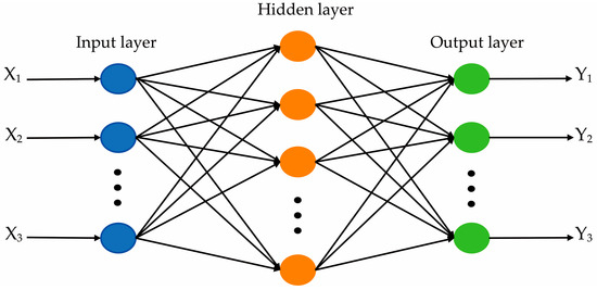
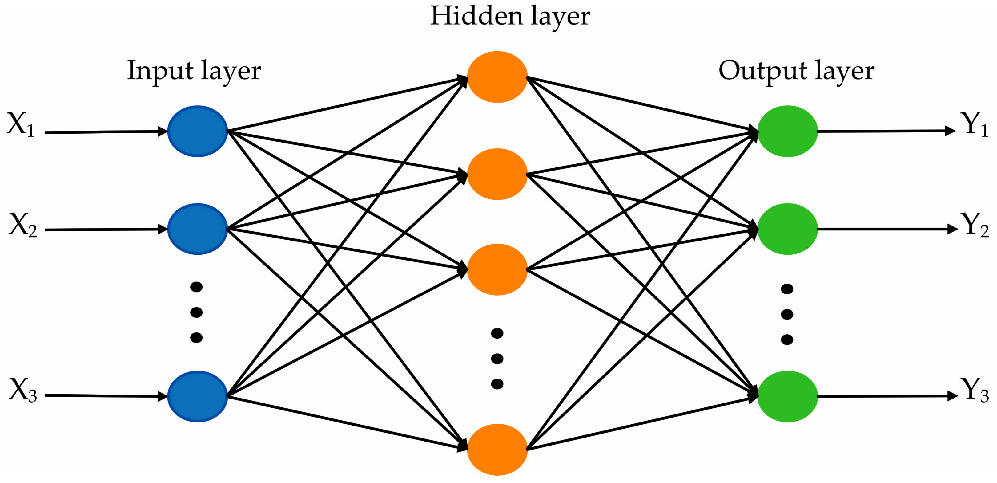
The Back Propagation Neural Network (BPNN) is a multi-layer feedforward neural network trained using the back propagation algorithm, and it remains one of the most classic and widely adopted models in the field [37]. As shown in Figure 1, a BPNN’s basic architecture consists of three layers: an input layer, a hidden layer and an output layer [38]. The input layer serves as the network’s data interface, receiving external input variables and transmitting them to the subsequent layer. The hidden layer performs feature extraction and nonlinear transformation, while the output layer produces the final prediction results. The network’s operation primarily involves two stages: forward propagation and error back propagation. During forward propagation, sample data are fed into the network through the input layer. They are then processed via weighted summation and activation functions in the hidden layer. Finally, the predicted output values are obtained at the output layer. In the error backpropagation stage, the error between the predicted output and the actual value is calculated. If this error does not meet the preset accuracy requirement, it is propagated backward, layer by layer, from the output layer to the hidden layer and then to the input layer. The gradient descent method is then applied iteratively to adjust the weights and thresholds of the neurons in each layer. This process progressively reduces the network’s prediction error.

Figure 1. Structure of the BP Neural Network.

2.2. SSA

The Sparrow Search Algorithm (SSA), proposed by Xue et al. in 2020, is a novel swarm intelligence algorithm inspired by the foraging and anti-predation behaviors of sparrows [39]. The algorithm’s specific procedure is as follows:

(1)

Initialize the population

The positions of the sparrows can be represented by the following matrix:

$$\begin{array}{c}X=\left[\begin{array}{cccc}{x}_{\mathrm{1,1}}& x_{\mathrm{1,2}}& \cdots & x_{1,d}\\ x_{\mathrm{2,1}}& x_{\mathrm{2,2}}& \cdots & x_{2,d}\\ ⋮& ⋮& ⋮& ⋮\\ x_{n,1}& x_{n,2}& \cdots & x_{n,d}\end{array}\right]\end{array}$$

(1)

where x_i,j represents the initial position of the i-th sparrow on the j-th dimensional decision variable, with i = 1, 2, …, n, and j = 1, 2, …, d; n denotes the population size and d is the dimension of the solution space.

(2)

Fitness value calculation

$$\begin{array}{c}{F}_x=\left[\begin{array}{c}f\left(\left[\begin{array}{cccc}{x}_{\mathrm{1,1}}& x_{\mathrm{1,2}}& \cdots & x_{1,d}\end{array}\right]\right)\\ f\left(\left[\begin{array}{cccc}{x}_{\mathrm{2,1}}& x_{\mathrm{2,2}}& \cdots & x_{2,d}\end{array}\right]\right)\\ ⋮\\ f\left(\left[\begin{array}{cccc}{x}_{n,1}& x_{n,2}& \cdots & x_{n,d}\end{array}\right]\right)\end{array}\right]\end{array}$$

(2)

(3)

Producer position update

$$\begin{array}{c}{X}_{i,j}^{t+1}=\left\{\begin{array}{ll}{X}_{i,j}^t·\mathit{exp}\left({\displaystyle \frac{-i}{\alpha ·ite{r}_{max}}}\right),& R_2<ST\\ X_{i,j}^t+Q·L,& R_2\ge ST\end{array}\right.\end{array}$$

(3)

where t represents the current iteration number, $X_{i,j}^t$ represents the current position of the i-th sparrow on the j-th dimensional decision variable at iteration t, α is a uniformly distributed random number in the interval [0, 1], iter_max is the maximum number of iterations of the algorithm, R² is the early warning value, ST is the safety threshold, Q is a random number following the normal distribution N(0, 1), and L is a matrix of dimension 1 × d.

(4)

Scrounger position update

$$\begin{array}{c}{X}_{i,j}^{t+1}=\left\{\begin{array}{ll}Q·\mathit{exp}\left({\displaystyle \frac{X_{worst}^t-X_{i,j}^t}{i^2}}\right),& i>{\displaystyle \frac{n}{2}}\\ X_p^{t+1}+\left|X_{i,j}^t-X_p^{t+1}\right|·A^{+}L,& i\le {\displaystyle \frac{n}{2}}\end{array}\right.\end{array}$$

(4)

where i represents the number of scroungers, n denotes the total number of sparrows, Xp and Xworst represent the optimal and worst positions in the current population, respectively; A is a d × d matrix whose elements are randomly assigned as 1 or −1; and A⁺ = A^T(AA^T)⁻¹.

(5)

Scout position update

$$\begin{array}{c}{X}_{i,j}^{t+1}=\left\{\begin{array}{ll}{X}_{best}^t+\beta ·\left|X_{i,j}^t-X_{best}^t\right|,& f_i>f_g\\ X_{i,j}^t+K·\left({\displaystyle \frac{\left|X_{i,j}^t-X_{worst}^t\right|}{\left(f_i-f_w\right)+\epsilon }}\right),& f_i=f_g\end{array}\right.\end{array}$$

(5)

where X_best is the optimal position of the sparrow, β is the step size control parameter, K belongs to the interval [−1, 1], f_i is the fitness value of the current individual in the population, f_g and f_w denote the global best and worst fitness values, respectively, and ε is a constant approaching zero which ensures that the denominator is non-zero.

2.3. Improved SSA

2.3.1. Tent Chaotic Mapping

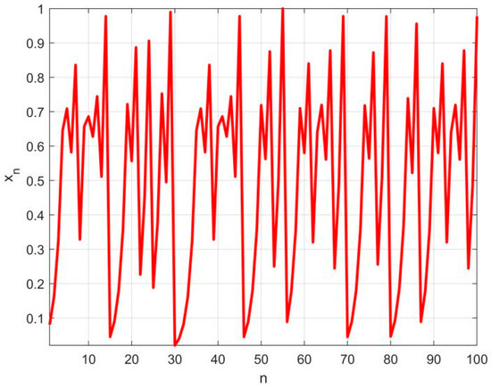
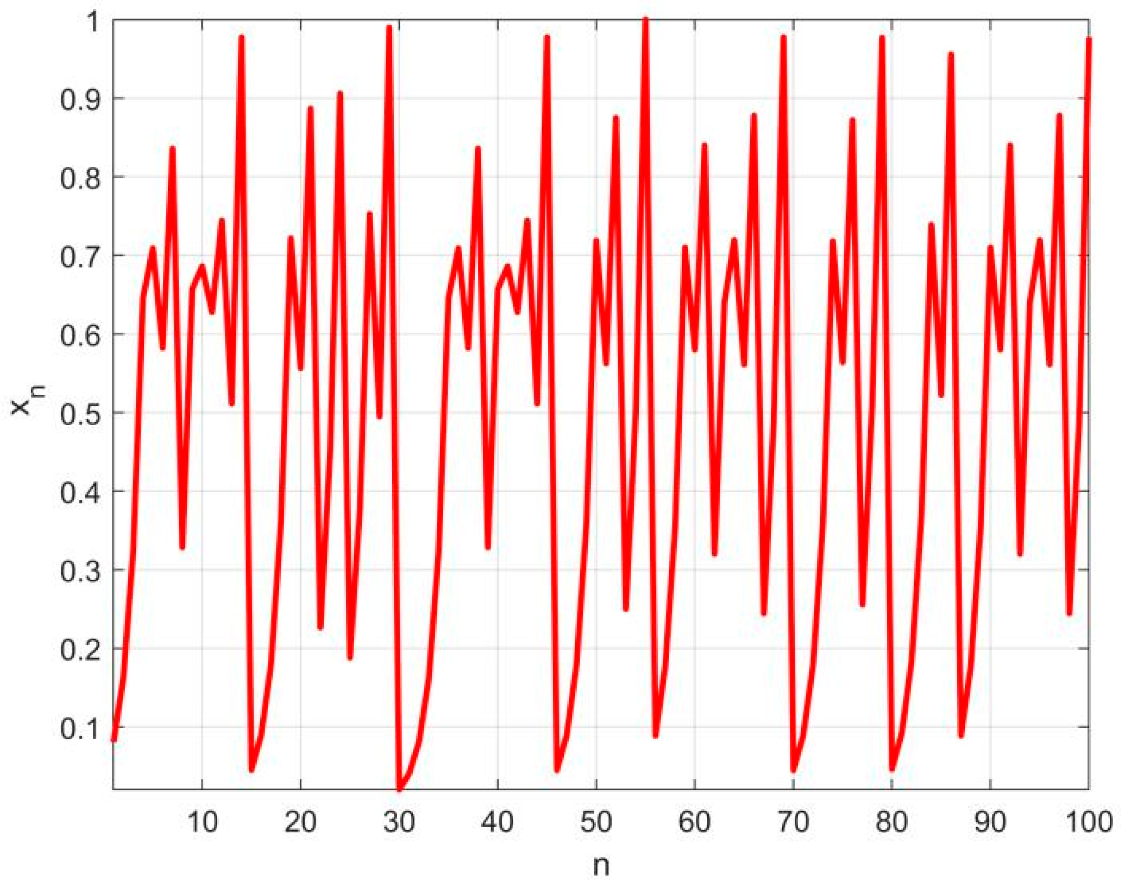
The initialization of the population in the original Sparrow Search Algorithm relies on a random generation strategy, which is highly stochastic and tends to result in an insufficiently diverse initial population. This degrades the algorithm’s optimization performance. To address this issue, this study proposes replacing the traditional random parameter generation method with Tent chaotic mapping. Tent chaotic mapping is a piecewise mapping characterized by good ergodicity, randomness and regularity [40]. Applying it to the population initialization stage effectively improves the diversity of the initial population, helping the algorithm escape local optima and enhancing its global search capability. The formulation of this chaotic mapping is as follows:

$$\begin{array}{c}{x}_{n+1}=\left\{\begin{array}{ll}2x_n,& 0\le x_n<{\displaystyle \frac{1}{2}}\\ 2\left(1-x_n\right),& {\displaystyle \frac{1}{2}}\le x_n\le 1\end{array}\right.\end{array}$$

(6)

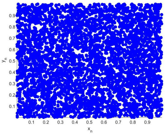
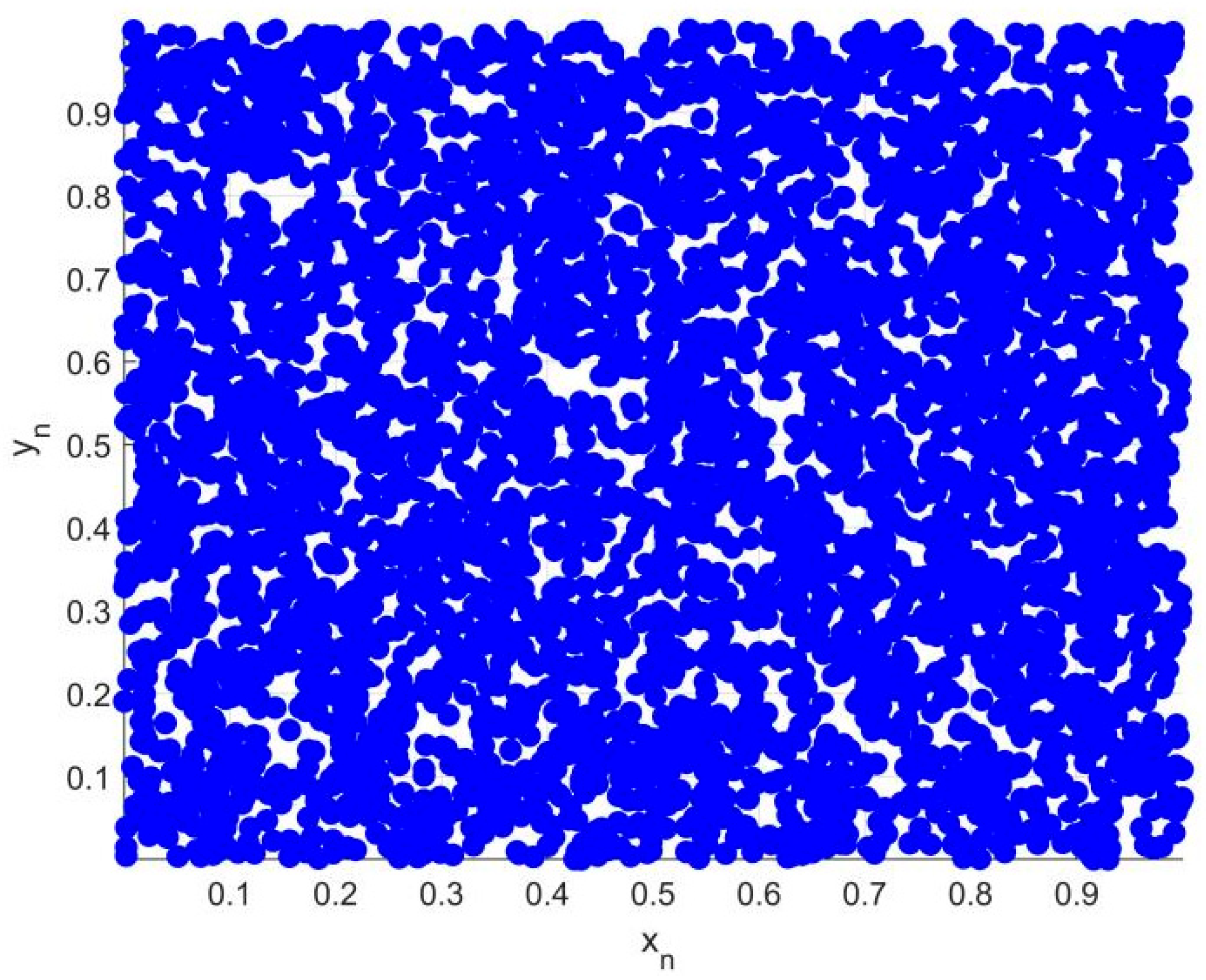
where n is the number of iterations and x_n is the chaotic sequence value at iteration n. Figure 2 shows the relationship between the Tent chaotic mapping and the number of iterations. Figure 3 shows the initial population after applying the Tent mapping. It can be seen that the mapped population essentially covers the entire space uniformly.

Figure 2. Relationship between Tent mapping and the number of iterations.

Figure 3. Distribution of the sparrow population after Tent mapping.

2.3.2. Dynamic Adaptive Weights

In the early stages of iteration, the producers gradually approach the globally optimal solution. However, if the search range is limited, the algorithm may easily become trapped in a local optimum. To address this issue, a dynamic adaptive weight factor is introduced into the producer position update formula. A higher weight value is assigned in the initial search stage to ensure sufficient global search capability. In the later stage, a lower weight value is adopted to enable a more refined local search and accelerate the algorithm’s convergence speed [41]. The expression of the weight coefficient is as follows:

$$\begin{array}{c}\omega =a\times {\left(1-{\left({\displaystyle \frac{t}{{Iter}_{max}}}\right)}^{\eta }\right)}^{{\displaystyle \frac{1}{\eta }}}\end{array}$$

(7)

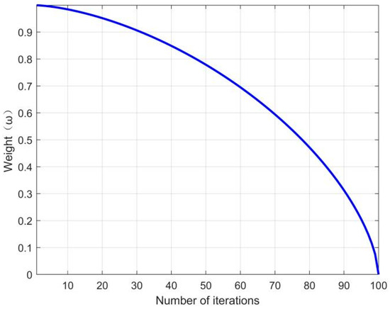
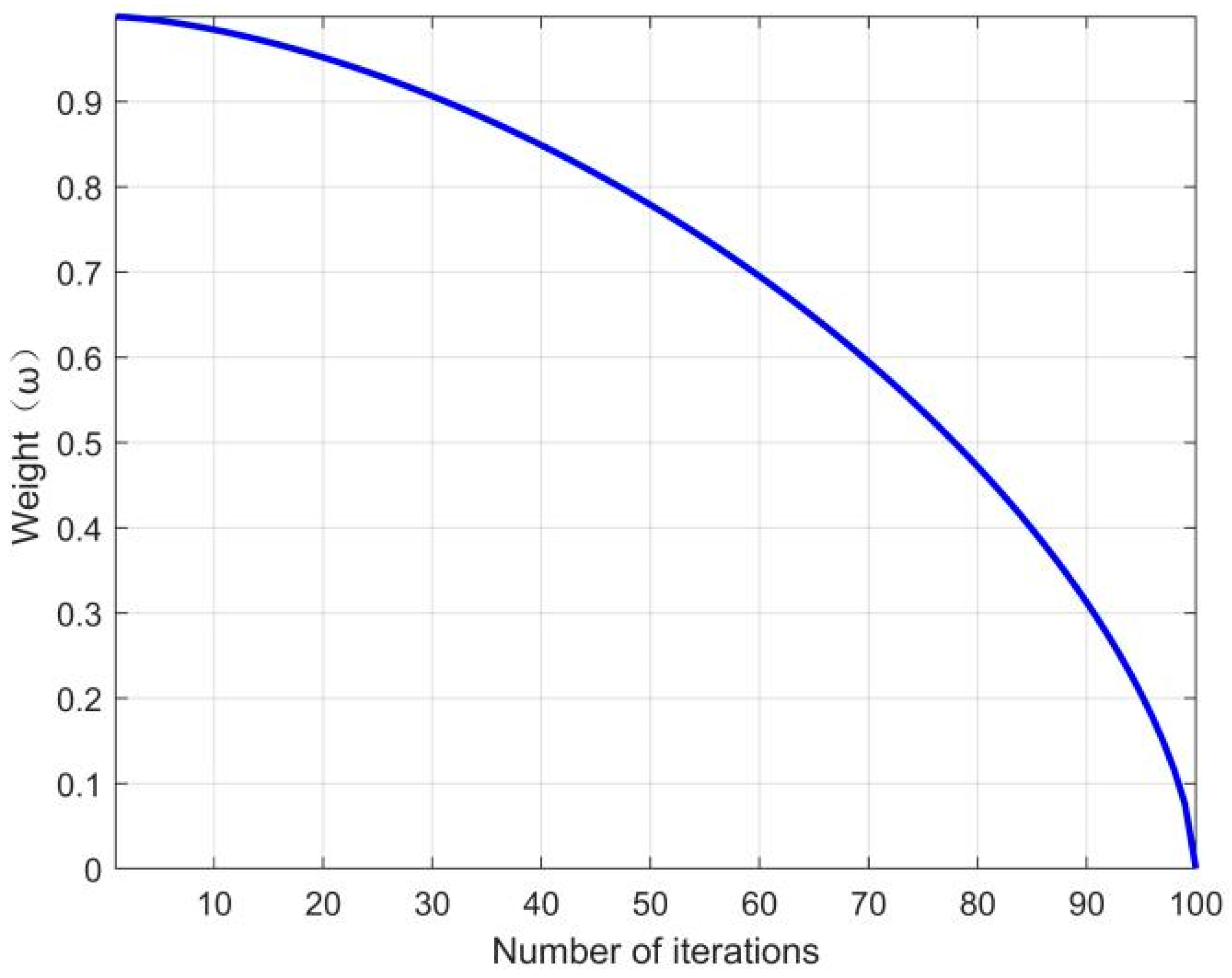
where a is a constant equal to 1, iter_max is the maximum number of iterations and η is the step size adjustment coefficient, set to 1.6. Equation (8) shows how the producer position is updated after the weight factor has been incorporated. Figure 4 shows the nonlinear decreasing trend of the weight coefficient as the number of iterations increases.

$$\begin{array}{c}{X}_{i,j}^{t+1}=\left\{\begin{array}{ll}{X}_{i,j}^t·\mathit{exp}\left({\displaystyle \frac{-\omega i}{\alpha ·ite{r}_{max}}}\right),& R_2<ST\\ X_{i,j}^t+Q·L,& R_2\ge ST\end{array}\right.\end{array}$$

(8)

Figure 4. Variation of the dynamic adaptive weight factor with the number of iterations.

2.4. ISSA-BP

The BP neural network has certain limitations during the training process. Since the network’s initial weights and thresholds are randomly generated, this can result in poor model stability and a tendency to fall into local optima. To address these issues, this paper uses the ISSA to optimize the BP neural network. Leveraging the ISSA’s strong global search capability, the algorithm optimizes the network’s initial weights and thresholds, replacing the traditional random assignment method. This allows the network to begin training with more favorable initial parameters, effectively avoiding local optima and enhancing its ability to generalize and predict.

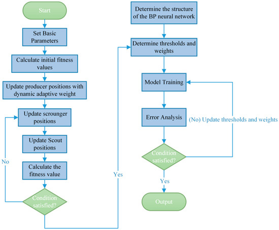
The steps specific to the ISSA-BP neural network model are as follows. The flowchart is shown in Figure 5.

Figure 5. Flowchart of the ISSA-BP model.

(1)

Determination of model inputs and outputs

According to the objective of residential building cost prediction, the screened engineering cost-influencing indicators are selected as the input variables of the model, while the unit cost of residential buildings is taken as the output variable. On this basis, the number of nodes in the input and output layers of the BP neural network is determined.

(2)

Data preprocessing

The qualitative indicators are first transformed into numerical variables, and both the input and output variables are subsequently normalized to reduce the influence of differences in dimensions and numerical ranges among indicators on network training. The dataset is then divided into training and testing sets using the hold-out method. The training set is used for model training and parameter optimization, whereas the testing set does not participate in the training process and is only used for the final evaluation of prediction performance.

(3)

Configuration of BP neural network structural parameters

The BP neural network is constructed according to the numbers of input and output variables. The structural and training parameters of the network are then determined, including the number of network layers, the number of hidden layers, the number of neurons in the hidden layer, the transfer function of the hidden layer, the transfer function of the output layer, and the training function. For the standard BP model, the initial weights and thresholds of the network are generated randomly. For the ISSA-BP model, the initial weights and thresholds are obtained through ISSA optimization.

(4)

Determination of ISSA optimization objects

The initial weights and thresholds of the BP neural network are taken as the optimization objects of ISSA, including the weights between the input layer and the hidden layer, the thresholds of the hidden layer, the weights between the hidden layer and the output layer, and the thresholds of the output layer. The dimension of the optimization variables is determined according to the topology of the BP neural network, and each sparrow individual is encoded as a complete set of initial BP weights and thresholds.

(5)

Setting of ISSA optimization parameters

The parameters of ISSA are specified, including the population size, the maximum number of iterations, parameter boundaries, the proportion of producers, the proportion of scroungers, the proportion of scouts, the safety threshold, and the termination criteria. These settings provide the basic conditions for the subsequent optimization process.

(6)

Initialization of the sparrow population

Tent chaotic mapping is adopted to generate the initial population, thereby improving the uniformity and ergodicity of the initial individuals in the search space. This strategy enhances the global search capability of the algorithm and reduces the influence of the randomness of population initialization on the optimization results.

(7)

Calculation of fitness values

The weights and thresholds represented by each sparrow individual are assigned to the BP neural network, and the network prediction error is calculated using the training set. The prediction error is used as the fitness function to evaluate the quality of each individual. A smaller fitness value indicates that the corresponding combination of initial weights and thresholds is more suitable for the BP neural network.

(8)

Updating of population positions

The individuals in the population are ranked according to their fitness values and are then divided into producers, scroungers, and scouts. Producers are responsible for guiding the global search, while scroungers update their positions according to the positions of producers. Scouts are introduced to enhance the ability of the algorithm to escape from local optima. Meanwhile, dynamic adaptive weights are incorporated into the position-updating process of producers to balance the global search capability in the early stage and the local optimization capability in the later stage of the algorithm.

(9)

Judgment of termination conditions

After each iteration, the fitness value of each individual is recalculated, and the current optimal individual is updated accordingly. When the predefined termination criterion is satisfied, the optimization process is stopped, and the global optimal individual is output. If the termination condition is not met, population updating and fitness calculation are continued.

(10)

Establishment of the ISSA-BP prediction model

The optimal individual obtained by ISSA is decoded into the initial weights and thresholds of the BP neural network and assigned to the BP network. On this basis, the BP neural network is trained using the training set, allowing the network parameters to be further adjusted through forward propagation and error backpropagation.

(11)

Model prediction and performance evaluation

The independent testing set is input into the trained ISSA-BP model to obtain the prediction results, which are then denormalized. Finally, multiple evaluation indicators are adopted to comprehensively assess the prediction accuracy, systematic bias, and stability of the model. The performance of the ISSA-BP model is further compared with that of the BP, GA-BP, WPA-BP, and SSA-BP models.

3. Algorithm Performance Test

To evaluate the performance of the improved Sparrow Search Algorithm (ISSA), three unimodal and five multimodal benchmark test functions were selected to evaluate the ISSA, Sparrow Search Algorithm (SSA), Wolf Pack Algorithm (WPA) and Genetic Algorithm (GA). The unimodal functions are F₁ to F₃, and the multimodal functions are F₄ to F₈. A unimodal function contains only one global optimum within the entire search space and has no local optima. Testing algorithms with unimodal functions enables their convergence speed, search accuracy and stability to be evaluated, providing an intuitive assessment of their efficiency in solving simple optimization problems and the precision of their solutions. In contrast, a multimodal function contains a global optimum and a large number of local optima within the search space, which makes optimization more challenging. Testing algorithms with multimodal functions enables their ability to escape local optimal, global search capability and robustness to be evaluated, providing an accurate reflection of their performance in avoiding premature convergence in complex problems. The population size for all algorithms is set to 100 and the number of iterations is also set to 100. To avoid errors caused by a single run, each of the four algorithms is executed 30 times on each of the eight benchmark test functions. The optimal, mean and standard deviation values are then calculated to evaluate the algorithms’ performance.

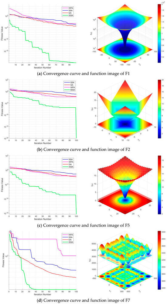
As shown in Table 1, for the unimodal functions F₁ to F₃, the average value obtained by ISSA is significantly smaller than that obtained by the other three algorithms. For the multimodal functions F₄ to F₈, the average value of ISSA on F₇ is close to that of GA, but slightly higher. On the other four multimodal functions, however, the average value of ISSA is significantly lower than that of the other algorithms. This indicates that ISSA exhibits excellent convergence accuracy. The standard deviation of ISSA on various benchmark functions is slightly inferior to that of WPA on the multimodal function F7, but is smaller than that of the other three algorithms on all other functions. This indicates that ISSA exhibits more excellent and stable performance in terms of stability compared to the other algorithms. Figure 6 presents the convergence curves and function images of some algorithms. As can be seen from Figure 6, ISSA outperforms the other algorithms in terms of both convergence speed and search accuracy on unimodal and multimodal functions alike.

Table 1. Comparison of the results of four algorithms on benchmark functions.

Function	Indicators	ISSA	SSA	WPA	GA
	best	1.064320 × 10−20	2.465685 × 10−3	1.685430 × 10−4	1.015801 × 10−5
F1	ave	4.416604 × 10−14	3.466380 × 10−2	1.918467 × 10−3	1.018117 × 10−3
	std	2.093543 × 10−13	3.692973 × 10−2	1.458000 × 10−3	1.748000 × 10−3
	best	2.864152 × 10−20	8.791292 × 10−2	6.090667 × 10−3	7.383166 × 10−3
F2	ave	8.913300 × 10−7	3.786109 × 10−1	5.527822 × 10−2	4.020333 × 10−2
	std	6.378849 × 10−6	2.405497 × 10−1	5.601500 × 10−2	2.840300 × 10−2
	best	1.839609 × 10−3	1.742739 × 10−1	1.084988 × 10−1	2.305404 × 10−1
F3	ave	1.008742 × 10−2	1.134062 × 100	2.890297 × 10−1	1.783001 × 100
	std	8.371705 × 10−3	6.688371 × 10−1	1.320750 × 10−1	8.253150 × 10−1
	best	1.011940 × 10−20	3.134367 × 100	2.035286 × 100	1.187583 × 10−1
F4	ave	1.320274 × 10−11	1.076044 × 101	8.415971 × 100	8.716129 × 100
	std	1.304081 × 10−10	6.891205 × 100	5.207894 × 100	6.778263 × 100
	best	4.440892 × 10−16	2.180659 × 10−2	8.178981 × 10−3	6.950520 × 10−3
F5	ave	1.981110 × 10−7	1.162224 × 100	1.360484 × 100	3.288378 × 10−1
	std	1.605013 × 10−6	8.710878 × 10−1	1.127977 × 100	7.014790 × 10−1
	best	1.008470 × 10−20	1.227765 × 10−3	3.518684 × 10−2	1.056633 × 10−5
F6	ave	6.845927 × 10−16	9.986020 × 10−3	2.219926 × 10−1	1.457342 × 10−3
	std	3.823230 × 10−15	1.093322 × 10−2	2.393785 × 10−1	3.538000 × 10−3
	best	5.329878 × 102	4.994440 × 102	9.106625 × 102	5.290320 × 102
F7	ave	1.022333 × 103	1.279043 × 103	1.469380 × 103	1.225960 × 103
	std	2.938188 × 102	3.082170 × 102	2.841631 × 102	3.768696 × 102
	best	1.558146 × 10−10	3.005981 × 10−3	1.192266 × 10−4	6.982707 × 10−6
F8	ave	3.302344 × 10−7	1.176247 × 10−1	7.764030 × 10−1	2.025245 × 10−4
	std	7.982022 × 10−7	7.514123 × 10−2	9.692840 × 10−1	2.120000 × 10−4

Figure 6. Convergence curves and function images of different test functions.

Therefore, ISSA generally outperforms the other three algorithms in terms of convergence accuracy, stability and speed. It exhibits stronger global optimization capabilities for unimodal functions and is better able to escape local optima for multimodal functions.

4. Establishment of Engineering Indicators

4.1. Preliminary Selection of Indicators

The preliminary screening of input variables was conducted based on three principles: literature analysis, verification of engineering significance, and examination of data availability. First, according to the influencing factors frequently identified in studies related to building cost estimation, indicators such as project scale, structural system, foundation type, decoration practice, and price index were initially selected. Then, in combination with the cost formation mechanism of residential buildings, variables capable of reflecting project quantity scale, technical characteristics, and market price fluctuations were retained. Finally, indicators that were difficult to obtain consistently or exhibited large differences in statistical caliber across projects were excluded. As a result, 18 initial cost-influencing factors were determined, as shown in Table 2.

Table 2. Indicator system for estimating residential building costs.

Serial Number	Indicators	Unit	Serial Number	Indicators	Unit
X1	Total floor area	m2	X10	Roof waterproofing	-
X2	Site area	m2	X11	Roof insulation	-
X3	Number of stories	floor	X12	Exterior wall decoration	-
X4	Above-ground floor height	m	X13	Wall insulation	-
X5	Seismic grade	grade	X14	Floor decoration	-
X6	Seismic fortification intensity	degree	X15	Interior wall decoration	-
X7	Structure type	-	X16	Door and window works	-
X8	Foundation type	-	X17	Proportion of grade III steel reinforcement by mass	%
X9	Roof form	-	X18	engineering cost index	-

Note: “-“ denotes a dimensionless indicator.

To clarify the meanings of the influencing factors listed in Table 2 and the unit cost, the definitions of these indicators are specified as follows.

(1)

Total floor area: refers to the sum of the horizontal projected areas of all floors of a building, including both above-ground and underground floor areas.

(2)

Site area: refers to the land area occupied by the ground floor of a building, namely the building footprint area.

(3)

Number of stories: refers to the number of above-ground floors of a building.

(4)

Above-ground floor height: refers to the vertical height between above-ground floors of a building, measured as the vertical distance from one floor level to the floor level above.

(5)

Seismic grade: refers to the seismic detailing grade determined according to the importance of the building and the seismic fortification requirements, generally classified from Grade I to Grade IV.

(6)

Seismic fortification intensity: refers to the expected level of seismic influence that a building may experience in its region, which is determined by the location of the project site.

(7)

Structure type: refers to the category of structural system adopted in a building, mainly including frame structures, shear wall structures, and frame-shear wall structures.

(8)

Foundation type: refers to the bottom structural form that bears the loads from the superstructure and transfers them to the ground, generally including raft foundations and pile foundations.

(9)

Roof form: refers to the structural form adopted for the building roof, mainly including flat roofs and pitched roofs.

(10)

Roof waterproofing: refers to the design grade and construction practice of the roof waterproofing works.

(11)

Roof insulation: refers to parameters such as the material type and thickness of the roof insulation layer, reflecting the thermal performance requirements of the roof.

(12)

Exterior wall decoration: refers to the finishing materials and decorative forms adopted for the exterior façade of a building, such as coatings, facing tiles, stone curtain walls, and glass curtain walls.

(13)

Wall insulation: refers to the material type and thickness of the external wall insulation system, such as EPS boards, XPS boards, and rock wool boards.

(14)

Floor decoration: refers to the floor finishing practices adopted on each floor of a building, such as cement mortar flooring, ceramic tile flooring, and wood flooring.

(15)

Interior wall decoration: refers to the decorative treatment applied to the interior wall surfaces of a building, such as plastering and coating, tile facing, and decorative panels.

(16)

Door and window works: refers to the material, form, and related attributes of exterior windows and doors, such as aluminum alloy windows, plastic-steel windows, and security doors.

(17)

Proportion of grade III steel reinforcement by mass: refers to the proportion of HRB400 reinforcement, namely grade III steel reinforcement, in the total mass of steel reinforcement used in the building structure.

(18)

Engineering cost index: refers to an index that comprehensively reflects the influence of price fluctuations in labor, materials, machinery, and other cost components on engineering cost relative to a base period. It reveals the temporal variation trend of construction project costs and is used to measure cost fluctuations across different periods. Since the data samples in this study are residential building projects in Sichuan Province from 2019 to 2024, the engineering cost indices from 2019 to 2024 were collected from the Sichuan Engineering Cost Information Network (http://www.sceci.net/index.html, accessed on 30 November 2025). The index is a fixed-base index with 2005 as the base period, where the engineering cost index in 2005 is set as 100.

(19)

Unit cost: refers to the construction and installation cost per unit floor area, calculated by dividing the total construction and installation cost by the total floor area. It is used as the prediction output variable in this study.

Based on the established indicator system for residential building cost estimation, data on the relevant indicators of case projects were collected. Significant differences exist in policy environments, geological conditions, and other fundamental factors across different regions; however, within the same region, various construction conditions are relatively similar, which can provide a stable and consistent data foundation for model training [42]. Therefore, this study takes Sichuan Province as the research area and collects data from 70 residential building projects. As the selected indicators consist of qualitative and quantitative variables, and the prediction model requires numerical values as input, the qualitative indicators must be quantified. This paper adopts a numerical encoding method, whereby natural numbers starting from 1 are assigned to the qualitative indicators. As shown in Table 3. Furthermore, due to the significant differences in magnitude among the various indicators, feeding them directly into the model could increase training time and slow down convergence speed. Therefore, the min–max normalization method is employed to normalize the data. The formula is as follows:

$$\begin{array}{c}{y}_i={\displaystyle \frac{x_i-x_{min}}{x_{max}-x_{min}}}\left(i=1,2,3,\dots \right)\end{array}$$

(9)

where x_min and x_max are the minimum and maximum values in the row where x is located, respectively.

Table 3. Quantification of qualitative indicators.

Code	Seismic Grade	Structure Type	Foundation Type	Roof Form	Roof Waterproofing	Roof Insulation	Exterior Wall Decoration
1	Grade I	Frame structure	Raft foundation	Flat roof	Membrane waterproofing	XPS	Coating
2	Grade II	Shear wall structure	Pile foundation	Tile roof	Coating waterproofing	XPS + PE	Coating + curtain wall
3	Grade III	Frame-shear wall structure			Composite waterproofing	NC-EPSIB	Coating + facing finish
4	Grade IV						Coating + stone finish
Code	Wall Insulation	Floor Decoration	Interior Wall Decoration		Windows		Doors
1	XPS	Cement mortar flooring	Coating		Plastic-steel windows		Plastic-steel doors
2	FCB	Tile flooring	Facing finish		Aluminum alloy windows		Aluminum alloy doors
3	EVIB	Sheet flooring	Coating + facing finish		Thermal-break aluminum alloy windows		Thermal-break aluminum alloy doors
4	CSIB	Coated flooring	Coating + panel finish				Solid wood doors
5	NCPSIB						Fire-rated doors
6	XPS + RWIB						Steel fire-rated doors
7	XPS + FCB
8	XPS + EVIB

Note: 1. XPS denotes Extruded Polystyrene Board; PE denotes Polyethylene Film; NC-EPSIB denotes Non-combustible Composite Expanded Polystyrene Insulation Board; FCB denotes Foam Cement Board; EVIB denotes Expanded Vitrified Microsphere Inorganic Insulation Board; CSIB denotes Composite Silicate Insulation Board; NCPSIB denotes Non-combustible Composite Polystyrene Insulation Board; and RWIB denotes Rock Wool Insulation Board. 2. Since door and window works involve various combinations of doors and windows, doors and windows are encoded separately in the table.

4.2. Final Selection of Indicators

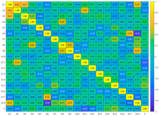
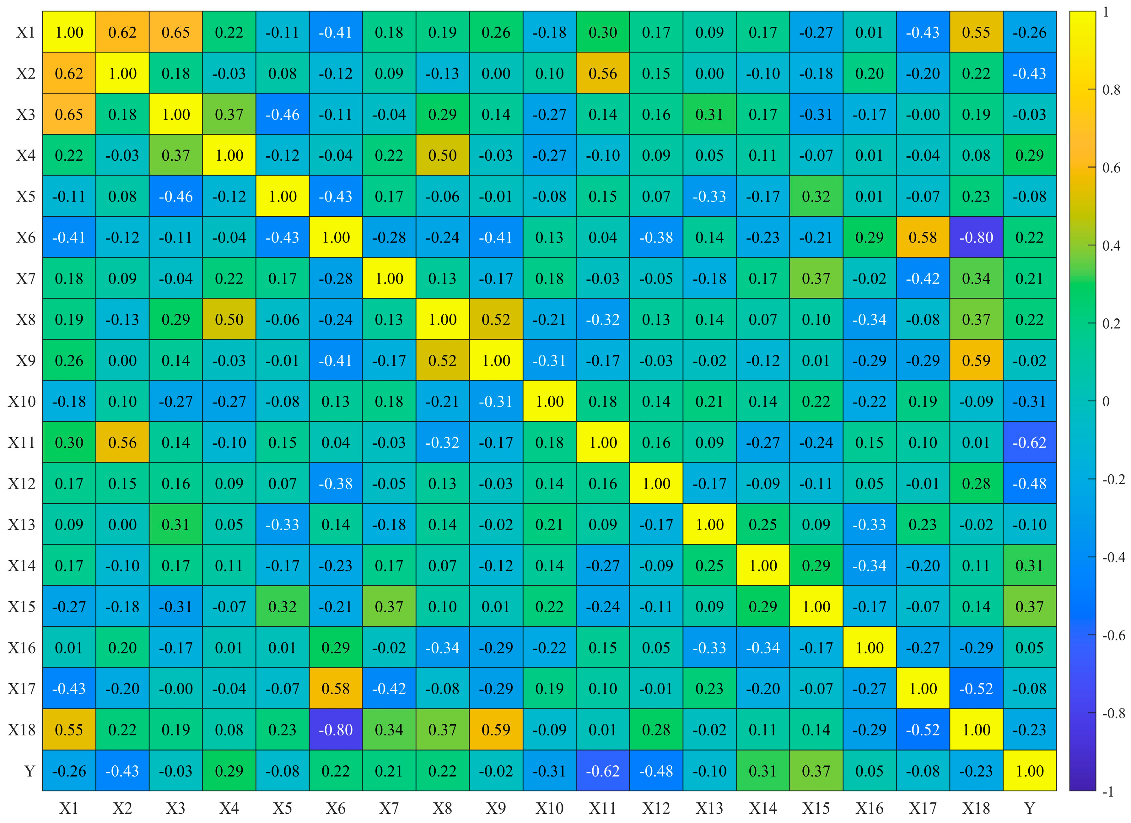
To analyze the correlations and potential redundancy among the initial input indicators, a correlation heatmap was plotted for the 18 initial input indicators and the output variable, namely the unit cost Y. The results are shown in Figure 7. Certain correlations were observed among some input indicators. For example, the correlation coefficient between seismic fortification intensity and the engineering cost index was −0.80, while the correlation coefficients between total floor area and number of stories, and between total floor area and site area, were 0.65 and 0.62, respectively. These results indicate that a certain degree of information overlap and potential redundancy exists in the original indicator system. In terms of the correlations between the input indicators and the unit cost, the strength of association varied across different indicators. Among them, roof insulation, exterior wall decoration, site area, and interior wall decoration showed relatively strong correlations with the unit cost. Therefore, the heatmap analysis was used as a preliminary basis for feature screening, and principal component analysis was further employed to select the initial indicators.

Figure 7. Correlation heatmap of input features and unit cost.

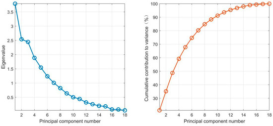
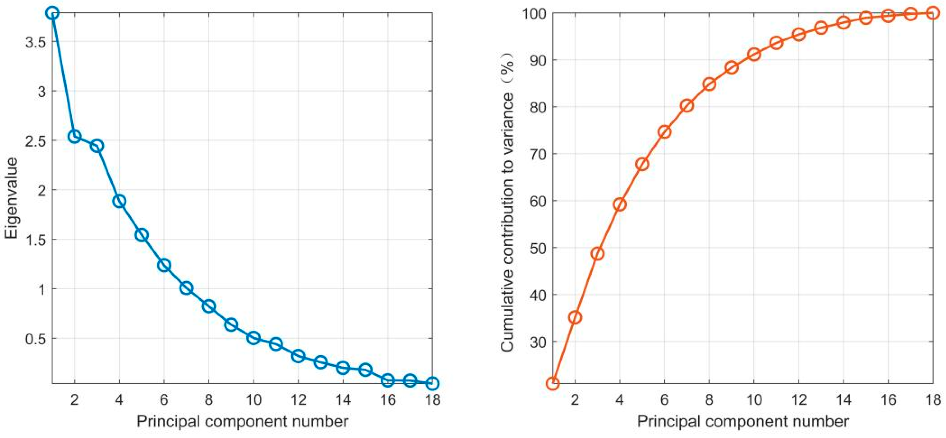
On the basis of the correlation analysis, a principal component analysis (PCA) was performed on the indicators using MATLAB R2024b. The results are presented in Table 4. In general, principal components with a cumulative variance contribution rate of 85% or higher are extracted. As can be seen in Table 3, the cumulative variance contribution rate of the first nine principal components is 88.3708%, which indicates that these nine components contain most of the information and meet the requirement. Therefore, the first nine principal components are extracted in this study. Figure 8 provides a more intuitive illustration of the variation in eigenvalues and cumulative variance contribution rates.

Table 4. Eigenvalues and contribution rates of principal components.

Principal Component	Eigenvalue	Eigenvalue Difference	Variance Contribution (%)	Cumulative Variance Contribution (%)
1	3.7882	1.2489	21.0453	21.0453
2	2.5392	0.0946	14.1069	35.1522
3	2.4446	0.5595	13.5813	48.7335
4	1.8852	0.3404	10.4731	59.2066
5	1.5447	0.3076	8.5818	67.7884
6	1.2371	0.2295	6.8729	74.6612
7	1.0076	0.1843	5.5980	80.2592
8	0.8233	0.1865	4.5739	84.8331
9	0.6368	0.1339	3.5377	88.3708
10	0.5029	0.0616	2.7941	91.1649
11	0.4414	0.1213	2.4520	93.6169
12	0.3201	0.0625	1.7783	95.3952
13	0.2575	0.0569	1.4308	96.8260
14	0.2007	0.0199	1.1150	97.9409
15	0.1808	0.1058	1.0047	98.9456
16	0.0750	0.0021	0.4168	99.3624
17	0.0729	0.0311	0.4053	99.7677
18	0.0418		0.2323	100.0000

Figure 8. Scree plot and cumulative variance contribution rate plot of principal component analysis.

In this principal component analysis, the KMO and SMC tests were employed to validate the analysis results. As shown in Table 5, the KMO test measures the correlation among indicators, with values ranging from 0 to 1; a higher value indicates stronger correlation, whereas a lower value indicates weaker correlation. The SMC value represents the commonality and linear relationship among indicators: the larger the SMC value, the stronger the commonality and linear relationship. The indicators basically meet the requirements, indicating that the dataset is suitable for principal component analysis.

Table 5. KMO and SMC values of the indicators.

Indicators	KMO	SMC
1	0.7697	0.8606
2	0.7666	0.6490
3	0.6786	0.8022
4	0.7254	0.5014
5	0.4848	0.7729
6	0.6505	0.9173
7	0.4806	0.7215
8	0.6307	0.7182
9	0.5577	0.8220
10	0.6346	0.6065
11	0.7155	0.5751
12	0.3634	0.6857
13	0.5412	0.5362
14	0.5956	0.5789
15	0.5804	0.5847
16	0.4730	0.7914
17	0.5591	0.8533
18	0.8448	0.8485
Total	0.6385

After determining the principal components, the factor score coefficient matrix was used to derive the expression for each component, labeled F1 to F9. The expressions are as follows:

F1 = 0.376816 ∗ x₁ + 0.154445 ∗ x₂ + 0.228275 ∗ x₃ + 0.160496 ∗ x₄ + 0.0621883 ∗ x₅ − 0.418787 ∗ x₆ + 0.184719 ∗ x₇ + 0.277826 ∗ x₈ + 0.296547 ∗ x₉ − 0.131076 ∗ x₁₀ − 0.008403 ∗ x₁₁ + 0.147202 ∗ x₁₂ − 0.00874595 ∗ x₁₃ + 0.122186 ∗ x₁₄ + 0.0337746 ∗ x₁₅ − 0.129133 ∗ x₁₆ − 0.318546 ∗ x₁₇ + 0.452302 ∗ x₁₈.

The expressions for the remaining eight principal components, from F₂ to F₉, can be derived by analogy. Once the expressions for all nine principal components have been obtained, the indicators contributing significantly to the calculation of each component are screened based on the absolute values of the factor score coefficients. These indicators are then used as input variables for the subsequent model. In this paper, the three indicators with the highest absolute weight coefficient values in each expression are selected, resulting in a total of 15 indicators. These are: Total floor area, site area, above-ground floor height, seismic grade, structure type, foundation type, roof form, roof waterproofing, exterior wall decoration, wall insulation, floor decoration, interior wall decoration, door and window works, proportion of grade III steel reinforcement by mass, and engineering cost index. This procedure not only preserves the main information contained in the original indicator system but also reduces information overlap among certain variables, thereby providing a more concise input variable system for subsequent model training.

5. Model Prediction and Comparative Analysis

5.1. BP Neural Network Model Prediction

The BP neural network model was constructed using MATLAB R2024b. First, to eliminate the influence of differences in dimensions and numerical ranges among different input indicators on model training, the min–max normalization method was applied to normalize both the input and output variables. After model prediction, the predicted outputs were denormalized to obtain the predicted unit cost of residential buildings at the original scale. In this study, an independent hold-out testing set was adopted to divide the sample data into training and testing subsets. A total of 70 residential building samples were divided into the training set and testing set at a ratio of approximately 7:3. The training set was used for network training of the BP neural network and the four coupled models, while the testing set was used for the final evaluation of prediction performance. According to the feature screening results obtained in the preceding analysis, the number of neurons in the input layer of the BP neural network was set to 15, corresponding to the 15 cost-influencing indicators. The number of neurons in the output layer was set to 1, corresponding to the unit cost of residential buildings. The network adopted a three-layer feedforward structure with a single hidden layer. The number of neurons in the hidden layer can generally be determined using Equation (10). Based on the analysis, five neurons were selected for the hidden layer in this study; therefore, the network topology was determined as 15-5-1. The tansig function was used as the transfer function of the hidden layer to enhance the network’s ability to fit nonlinear relationships, while the purelin linear function was adopted as the transfer function of the output layer to accommodate continuous numerical prediction outputs. The trainscg function was used as the network training function. The maximum number of training epochs was set to 1000, and the target training error was set to 0.01.

In this study, the coefficient of determination (R2), root mean square error (RMSE), mean absolute error (MAE), mean absolute percentage error (MAPE), and mean bias error (MBE) were selected as evaluation indicators. The corresponding calculation formulas are given in Equations (11)–(15).

$$\begin{array}{c}h=\sqrt{i+o}+a\end{array}$$

(10)

where i is the number of neurons in the input layer, o is the number of neurons in the output layer and a is an adjustment constant typically taking a value between 1 and 10.

$$\begin{array}{c}{R}^2=1-{\displaystyle \frac{{\displaystyle {\sum }_{i=1}^n}(y_i-{\widehat{y}}_i{)}^2}{{\displaystyle {\sum }_{i=1}^n}(y_i-\overline{y}{)}^2}}\end{array}$$

(11)

$$\begin{array}{c}RMSE=\sqrt{{\displaystyle \frac{1}{n}}{\displaystyle \sum _{i=1}^n}(y_i-{\widehat{y}}_i{)}^2}\end{array}$$

(12)

$$\begin{array}{c}MAE={\displaystyle \frac{1}{n}}{\sum }_{i=1}^n\left|y_i-{\widehat{y}}_i\right|\end{array}$$

(13)

$$\begin{array}{c}MAPE={\displaystyle \frac{1}{n}}{\displaystyle \sum _{i=1}^n}\left|{\displaystyle \frac{y_i-{\widehat{y}}_i}{y_i}}\right|\times 100\%\end{array}$$

(14)

$$\begin{array}{c}MBE={\displaystyle \frac{1}{n}}{\sum }_{i=1}^n\left(y_i-{\widehat{y}}_i\right)\end{array}$$

(15)

In the formula, y_i represents the actual value of the i-th sample, ${\widehat{y}}_i$ represents the predicted value of the i-th sample, $\overline{y}$ is the mean of the actual values, and n is the number of samples.

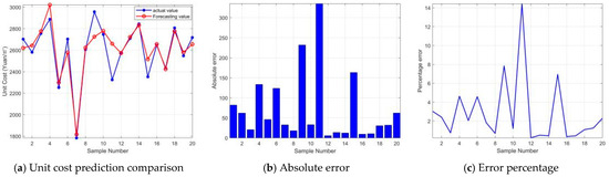
To validate the prediction accuracy of the BP neural network model for the unit construction cost of residential buildings, in this study, a representative single-run experiment was first conducted for the model. The comparison between the actual and predicted values of the testing samples, the absolute error distribution, and the percentage error distribution were then plotted, as shown in Figure 9. Regarding the fitting effect between the actual and predicted values in subfigure (a), it can be observed that the overall trend of the model’s predicted value curve is generally consistent with that of the actual value curve. Most sample points exhibit small deviations between the predicted and actual values, with only a few noticeable discrepancies occurring at samples 9, 11, and several others. Subfigure (b) further quantifies the prediction deviation of the model. Overall, the absolute errors of most samples are kept below 150 CNY/m², with over half of the samples having errors of less than 100 CNY/m². Three samples exhibit absolute errors exceeding 150 CNY/m², with the maximum absolute error surpassing 300 CNY/m². Only a few samples show relatively large errors. Subfigure (c) intuitively reflects the model’s prediction accuracy. Most samples have error percentages within 10%, with only one sample exceeding 14%. Further analysis based on the model’s evaluation metrics shows that the coefficient of determination (R²) is 0.8179, indicating a good model fit. The root mean square error (RMSE) is 111.3925 CNY/m² and the mean absolute percentage error (MAPE) is 2.8495%. Both of these fall within a reasonable range for engineering cost estimation. A comprehensive analysis of the figures and evaluation metrics reveals that the BP neural network model effectively captures the overall variation pattern of cost data, achieving relatively high prediction accuracy for most samples. However, the model exhibits insufficient fitting capability for a few individual samples, resulting in relatively large local prediction errors. Therefore, the model still needs to be improved.

Figure 9. Prediction plots of the BP neural network.

5.2. Comparative Analysis of Improved BP Models

This study improves the BP neural network model using different algorithms and establishes four combined models: GA-BP, WPA-BP, SSA-BP and ISSA-BP. To ensure the fairness and consistency of model comparison, the common experimental conditions of the five models were uniformly controlled in this study. All models adopted the same data partitioning scheme, input variables, BP network structure, training function, and evaluation indicators. For the four optimization algorithms, the initial weights and thresholds of the BP neural network were taken as the optimization objects, and the optimization dimension, population size, maximum number of iterations, parameter boundaries, and termination criteria were uniformly specified. The population size for each optimization algorithm is set to 100 and the maximum number of iterations is also set to 100. Since the topology of the BP neural network was 15-5-1, each optimization algorithm was required to optimize the weights between the input layer and the hidden layer, the thresholds of the hidden layer, the weights between the hidden layer and the output layer, and the threshold of the output layer. Therefore, the optimization dimension was calculated as 15 × 5 + 5 + 5 × 1 + 1 = 86, and the parameter boundaries were uniformly set to [−1, 1]. The termination criterion was defined as reaching the maximum number of iterations. When the number of iterations reached 100, the optimization process was stopped, and the current global optimal individual was output as the initial weights and thresholds of the BP neural network. For GA, the crossover probability is set to 0.8 and the mutation probability is dynamically adjusted using the adaptive mutation function, mutation_adaptive_feasible. The selection strategy is the elite retention strategy with an elite count of 10% of the population size; For WPA, the wandering step size adopts an adaptive Levy step size with LevyScale = 0.2 × (1 − t/T_max). The running step size is determined by a movement coefficient A = 0.1 × (2 × a × r1 − a), where a decreases linearly from 2 to 0. The proportions of scout wolves, fierce wolves, and leader wolves follow a three-wolf (alpha, beta, delta) guidance mechanism, and the top three elite wolves are retained; For SSA, the proportion of producers is set to 0.2, the proportion of scouts is set to 0.5, and the safety threshold is set to 0.8; For ISSA, the proportion of producers is adaptive, decreasing linearly from 0.5 to 0.2; the proportion of scouts is adaptive, calculated as 0.1 + 0.1 × rand, where rand is a random number between 0 and 1, and the safety threshold is adaptive, calculated as 0.6 + 0.2 × rand.

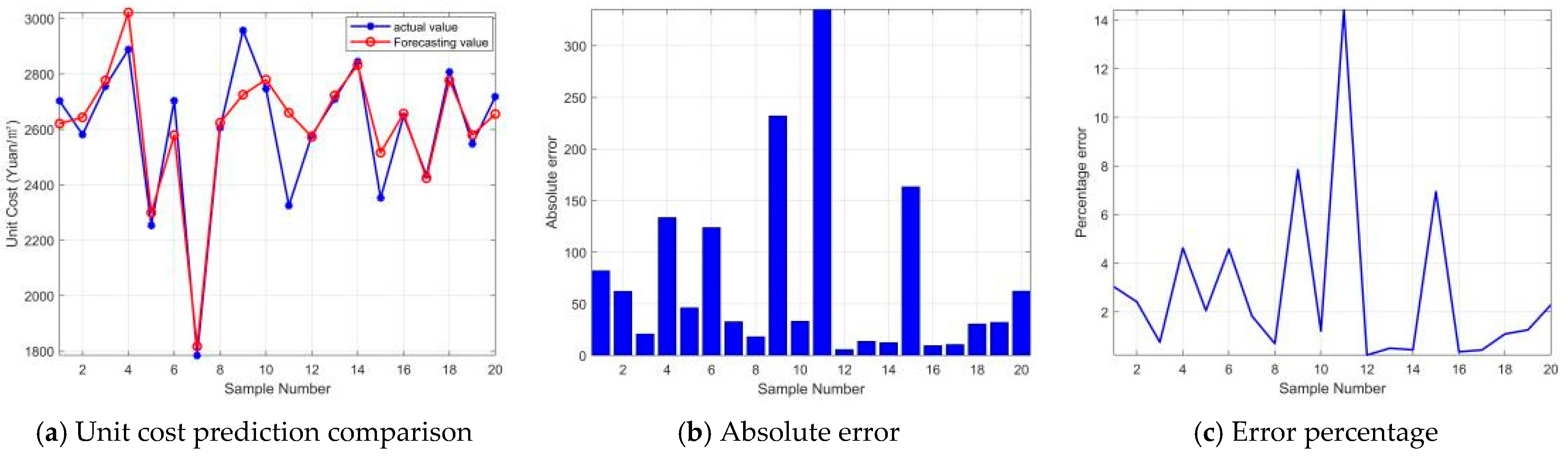
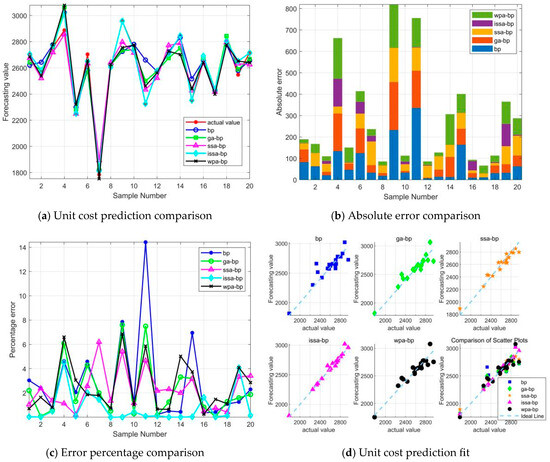
Figure 10 presents the prediction results, absolute errors, percentage errors, and fitting performance of the BP, GA-BP, WPA-BP, SSA-BP, and ISSA-BP models on the testing set. As shown by the prediction curves, the standalone BP model exhibits noticeable deviations from the actual values for several samples, indicating its limited local fitting capability for individual cases. Compared with the BP model, the GA-BP and WPA-BP models show certain improvements; however, prediction fluctuations are still observed for some samples. The prediction curve of the SSA-BP model is generally closer to the actual values, suggesting that the optimization of the initial BP parameters by SSA can improve the predictive performance of the model. In contrast, the predicted values of the ISSA-BP model show the highest degree of agreement with the actual values, while its absolute errors and percentage errors remain at relatively low levels. This indicates that, after introducing Tent chaotic mapping and dynamic adaptive weights, ISSA can further enhance the parameter optimization capability of the BP neural network, thereby effectively reducing the local prediction deviations on the testing samples. To further quantify the prediction differences shown in Figure 10, Table 6 presents the evaluation results of the five models under a representative single run. As shown in Table 6, from the perspective of fitting ability, the ISSA-BP model achieves an R² of 0.9754, which is higher than those of BP, GA-BP, WPA-BP, and SSA-BP, indicating that it has the strongest explanatory capability for variations in the unit cost of residential buildings. In terms of absolute error, the RMSE and MAE of ISSA-BP are 40.9194 and 20.0025, respectively, both of which are lower than those of the other models, demonstrating its stronger ability to control both large errors and average errors. From the perspective of relative error, the MAPE of ISSA-BP is 0.7633%, indicating that its predicted results have the smallest relative deviation from the actual construction costs. Regarding systematic bias, GA-BP and SSA-BP exhibit relatively low mean net bias in this run, whereas BP, WPA-BP, and ISSA-BP show relatively high mean net bias. Overall, the ISSA-BP model demonstrates better prediction accuracy and generalization capability than the other models.

Figure 10. Prediction comparison of the five models.

Table 6. Comparison of evaluation metrics for the five prediction models.

Model	R2	RMSE	MAE	MAPE (%)	MBE
BP	0.8179	111.3925	72.9970	2.8495	17.0381
GA-BP	0.8877	87.4719	60.5894	2.2973	−0.4293
WPA-BP	0.8856	88.2915	66.6124	2.5387	0.8814
SSA-BP	0.9297	69.2262	57.4596	2.2737	−9.9070
ISSA-BP	0.9754	40.9194	20.0025	0.7633	11.9308

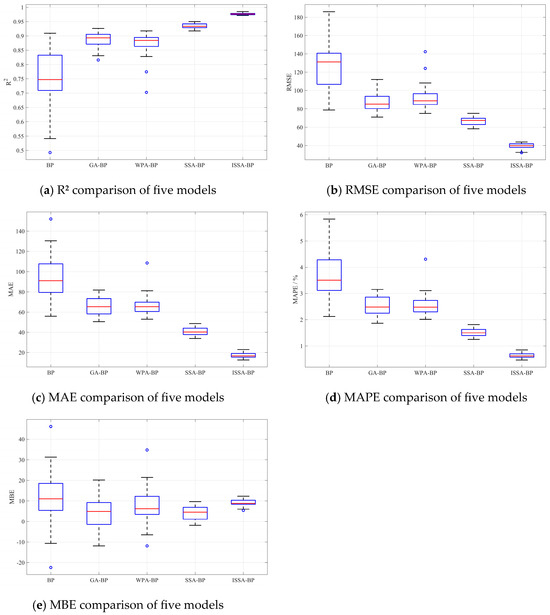
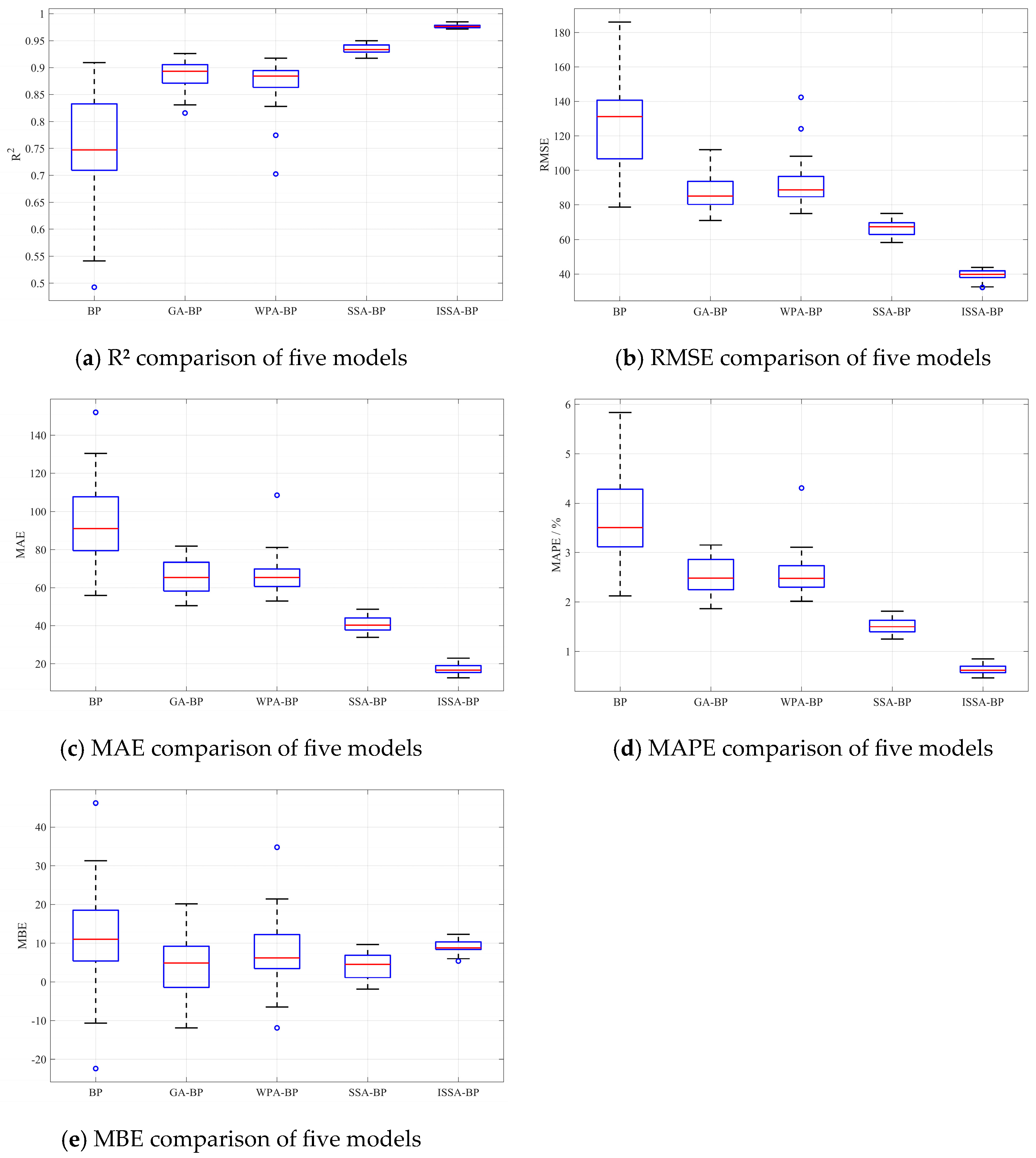
To further verify the generalization ability and stability of the models, 30 repeated experiments were conducted for the BP, GA-BP, WPA-BP, SSA-BP, and ISSA-BP models while maintaining the same training–testing data partitioning and evaluation indicator system. The mean and standard deviation of each evaluation indicator were then calculated, as shown in Table 7. Meanwhile, box plots were used to further illustrate the distribution characteristics of the five models under different evaluation indicators, as shown in Figure 11. Compared with the representative single-run results presented in Table 6, Table 7 and Figure 11 provide a more comprehensive reflection of the average predictive performance and result fluctuations of the models under random initialization and intelligent optimization search processes.

Table 7. Mean and standard deviation of evaluation metrics over 30 runs for five models.

Model	R2		RMSE		MAE		MAPE		MBE
	(Mean)	(Std)	(Mean)	(Std)	(Mean)	(Std)	(Mean)	(Std)	(Mean)	(Std)
BP	0.7541	0.0952	127.1722	24.6437	93.0378	20.1488	3.6321	0.7905	11.6031	13.5790
GA-BP	0.8879	0.0263	86.8481	9.9361	65.4160	8.6899	2.5085	0.3575	3.9545	7.5395
WPA-BP	0.8695	0.0429	93.3320	13.7335	67.1285	10.7023	2.5661	0.4398	7.7916	8.8852
SSA-BP	0.9343	0.0085	66.7651	4.3779	40.7513	3.8926	1.5067	0.1476	4.1693	3.3103
ISSA-BP	0.9773	0.0036	39.2339	3.2592	17.0973	2.2172	0.6293	0.0837	9.1583	1.6386

Figure 11. Evaluation indicator comparison of the five models over 30 runs.

As shown in Table 7, based on the average performance of the 30 repeated experiments, ISSA-BP exhibits the best performance in terms of both fitting ability and error control. Its mean R² value is 0.9773, which is higher than those of SSA-BP, GA-BP, WPA-BP, and BP, indicating that ISSA-BP has the strongest explanatory capability for the variation pattern of residential building unit costs. Further from the perspective of absolute error, the mean RMSE and MAE values of ISSA-BP are 39.2339 and 17.0973, respectively, both of which are noticeably lower than those of the other models. This suggests that ISSA-BP has a stronger ability to control both large errors and average errors. From the perspective of relative error, the mean MAPE of ISSA-BP is only 0.6293, indicating that the relative deviation between its predicted values and the actual costs is the smallest, making it more suitable for engineering cost estimation scenarios. In terms of stability, the standard deviation of R² for ISSA-BP is 0.0036, which is lower than that of the other four models. The standard deviations of its MAE, MAPE, and MBE are also at relatively low levels among the five models, indicating that ISSA-BP maintains more stable predictive performance across multiple independent runs. Combined with Figure 11, the R² box of ISSA-BP is located in a higher range, while the boxes of RMSE, MAE, and MAPE are located in lower ranges with relatively narrow widths. In contrast, BP, GA-BP, and WPA-BP exhibit more obvious outliers, suggesting that these models may be affected by local optima or insufficient search capability in individual runs, resulting in larger fluctuations in predictive performance. The main error indicators of ISSA-BP are more concentrated, and the degree of abnormal deviation is relatively small. This indicates that Tent chaotic mapping and dynamic adaptive weights can enhance the diversity of the initial population and improve the local search capability in the later stage, thereby reducing the model’s sensitivity to random initialization. These results further demonstrate that ISSA-BP not only achieves higher average prediction accuracy but also exhibits smaller operational fluctuations. Considering fitting ability, absolute error, relative error, systematic bias, and stability, ISSA-BP outperforms the other BP-based models in both major accuracy indicators and stability indicators. Therefore, it can be regarded as the prediction model with the best overall performance among the BP-based models.

5.3. Comparative Analysis of RF, XGBoost, and Their Optimized Models

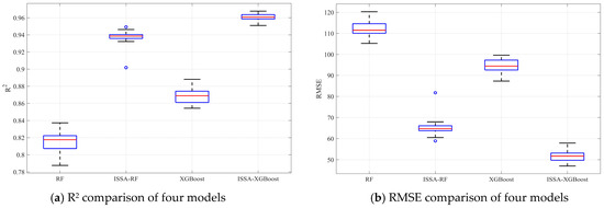
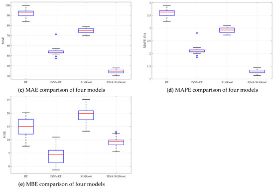
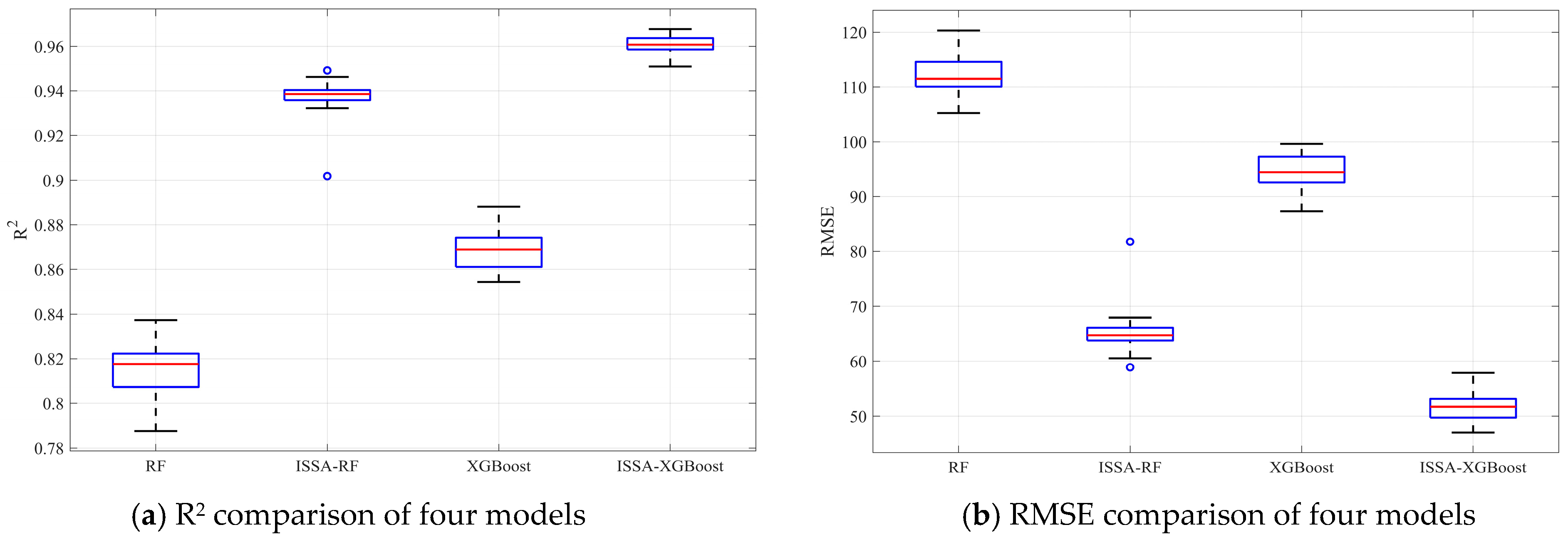
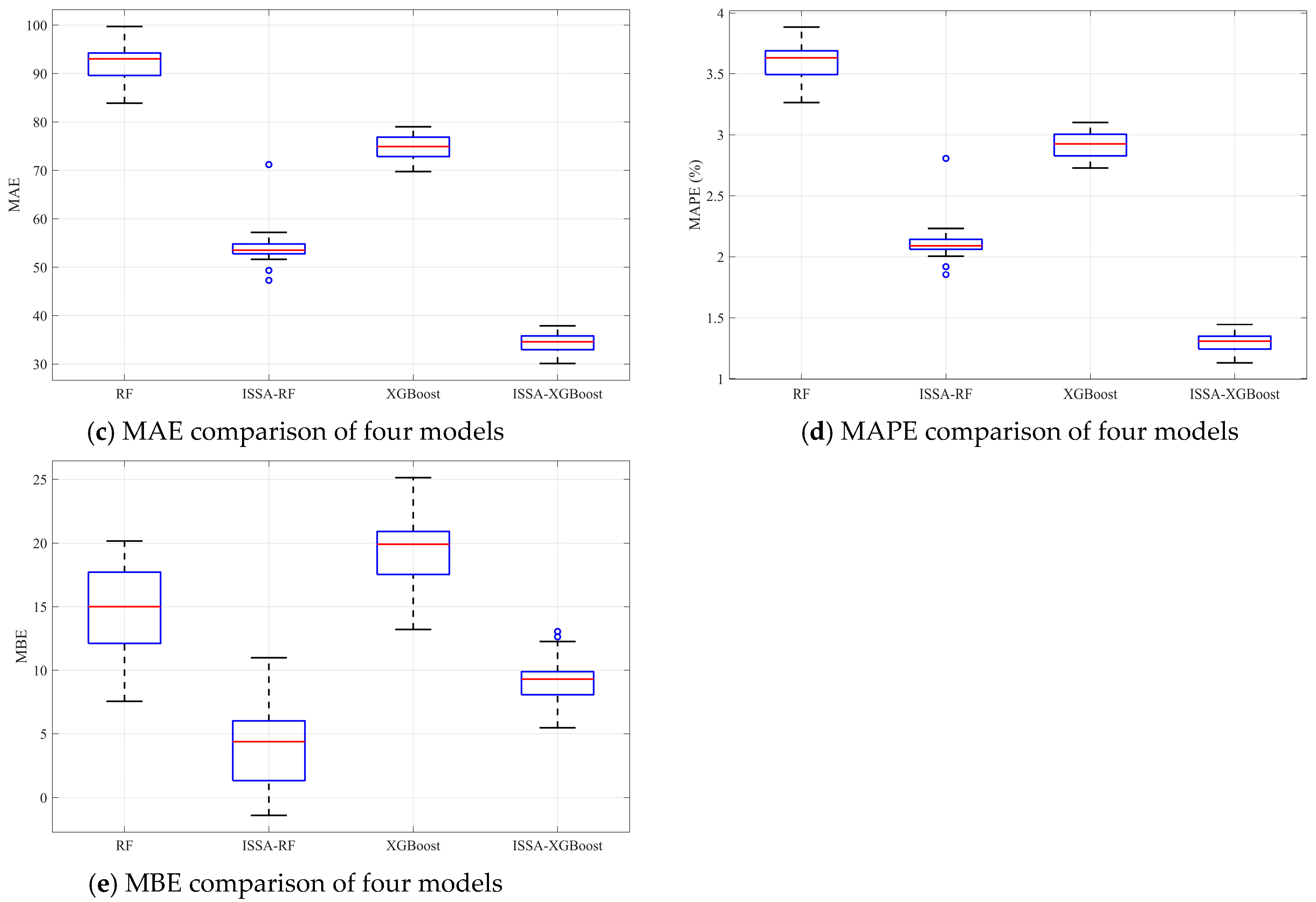
To further extend the comparison between the BP model and other types of machine learning models, and to verify the applicability of the proposed ISSA optimization method to different machine learning models, this study refers to the idea of constructing a multi-model comparison framework for complex engineering prediction problems proposed by Asgarkhani et al. [43]. Two ensemble learning models, namely Random Forest (RF) and Extreme Gradient Boosting (XGBoost), were introduced for comparative analysis, and the ISSA-RF and ISSA-XGBoost models were further developed. To ensure the fairness of model comparison, the four models adopted the same sample partitioning strategy, input variables, and evaluation metric system as the models described above. Meanwhile, the parameter settings of ISSA were kept consistent. However, because different models have different structures and parameters to be optimized, the optimization objects of ISSA also vary accordingly. For ISSA-BP, the optimization objects were the initial weights and thresholds of the BP neural network. For ISSA-RF and ISSA-XGBoost, the optimization objects were the key hyperparameters of RF and XGBoost, respectively. For the RF model, the number of trees was set to 100, the maximum depth was set to 10, the minimum number of samples per leaf node was set to 2, and both the feature sampling ratio and sample sampling ratio were set to 0.8. For the ISSA-RF model, the search range for the number of trees was set to 100–300, the maximum depth range was set to 3–12, the range of the minimum number of samples per leaf node was set to 2–8, the feature sampling ratio was set to 0.50–0.90, and the sample sampling ratio was set to 0.80–1.00. For the XGBoost model, the number of trees was set to 100, the maximum depth was set to 3, the learning rate was set to 0.1, and both the feature sampling ratio and sample sampling ratio were set to 0.8. For the ISSA-XGBoost model, the search range for the number of trees was set to 50–200, the maximum depth range was set to 2–6, the learning rate range was set to 0.03–0.20, the sample sampling ratio was set to 0.70–1.00, and the feature sampling ratio was set to 0.60–1.00. In this study, 30 independent repeated experiments were conducted for RF, ISSA-RF, XGBoost, and ISSA-XGBoost. The predictive performance and stability of the four models were comprehensively evaluated using evaluation metrics and boxplots, and the results are presented in Table 8 and Figure 12.

Table 8. Mean and standard deviation of evaluation metrics over 30 runs for four models.

Model	R2		RMSE		MAE		MAPE		MBE
	(Mean)	(Std)	(Mean)	(Std)	(Mean)	(Std)	(Mean)	(Std)	(Mean)	(Std)
RF	0.8160	0.0121	111.9221	3.6712	92.2005	3.9086	3.6013	0.1569	14.7648	3.2097
ISSA-RF	0.9377	0.0076	65.0752	2.8650	54.0375	3.0159	2.1118	0.1203	4.0012	2.5621
XGBoost	0.8683	0.0084	94.7005	3.0476	74.7277	2.4737	2.9242	0.0985	19.3926	2.7957
ISSA-XGBoost	0.9607	0.0038	51.6771	2.3379	34.3857	1.8912	1.2985	0.0739	9.2844	1.8491

Figure 12. Evaluation indicator comparison of the four models over 30 runs.

As shown in Table 8, from the perspective of fitting ability, the mean R² value of RF increased from 0.8160 to 0.9377 after ISSA optimization, while that of XGBoost increased from 0.8683 to 0.9607. This indicates that ISSA optimization can enhance the explanatory capability of the models for the variation pattern of residential building unit costs. In terms of absolute error, the mean RMSE and MAE values of RF decreased from 111.9221 and 92.2005 to 65.0752 and 54.0375, respectively, after optimization. Similarly, the mean RMSE and MAE values of XGBoost decreased from 94.7005 and 74.7277 to 51.6771 and 34.3857, respectively. These results demonstrate that the optimized models have a significantly improved ability to control both large errors and mean absolute errors. From the perspective of relative error, the mean MAPE values of RF and XGBoost decreased from 3.6013 and 2.9242 to 2.1118 and 1.2985, respectively, indicating that the relative prediction deviations of the models were further reduced after ISSA optimization. Regarding systematic bias, the mean MBE values of RF and XGBoost decreased from 14.7648 and 19.3926 to 4.0012 and 9.2844, respectively, suggesting that the overall tendency of overestimation or underestimation was weakened after optimization. From the perspective of stability, the standard deviations of all evaluation metrics for ISSA-RF and ISSA-XGBoost are lower than those of their corresponding original models, indicating that ISSA optimization not only improves the average predictive performance but also reduces the fluctuations in results across the 30 independent runs. Further comparison shows that ISSA-XGBoost outperforms ISSA-RF in the main accuracy indicators, including R², RMSE, MAE, and MAPE, suggesting that it achieves better overall predictive performance on the dataset used in this study. Figure 12 further verifies the results in Table 8 from the perspective of distribution. Compared with the original RF and XGBoost models, the R² boxes of ISSA-RF and ISSA-XGBoost shift upward overall, whereas the RMSE, MAE, and MAPE boxes shift downward. This indicates that the performance improvement of the optimized models is not caused by a few individual runs, but can be maintained in most repeated experiments. Meanwhile, the box widths and whisker lengths of the optimized models are generally reduced, suggesting that the dispersion of the evaluation metrics decreases and the operational stability of the models is enhanced. The MBE boxes also show a more concentrated distribution, indicating that the fluctuation in the models’ overall tendency toward overestimation or underestimation is weakened.

Further comparison of ISSA-RF and ISSA-XGBoost with ISSA-BP in Section 5.2 shows that, in terms of prediction accuracy, ISSA-BP performs noticeably better than both ISSA-RF and ISSA-XGBoost, as reflected by its higher mean R² and lower mean RMSE, MAE, and MAPE values. From the perspective of stability, the standard deviation of RMSE for ISSA-BP is slightly higher than that of ISSA-RF and ISSA-XGBoost, while the standard deviations of MAE and MAPE are slightly higher than those of ISSA-XGBoost. Nevertheless, considering both average prediction accuracy and operational stability, ISSA-BP remains the model with the best overall performance on the dataset used in this study.

Overall, ISSA optimization is not only effective for BP neural networks. Whether optimizing the initial weights and thresholds of BP or optimizing the hyperparameters of ensemble learning models such as RF and XGBoost, ISSA can improve model fitting ability, reduce error levels, and enhance operational stability to varying degrees. This indicates that ISSA has certain model adaptability and potential for further extension. However, because different models have different optimization objects and model structures, the degree of performance improvement also varies. For the 70 residential building cost samples used in this study, ISSA-BP still outperforms ISSA-RF and ISSA-XGBoost in the main prediction accuracy indicators. This suggests that, for small-sample and nonlinear residential building cost prediction problems, improving the initial parameters of the BP neural network through ISSA can achieve better overall predictive performance.

6. SHAP Interpretability Analysis

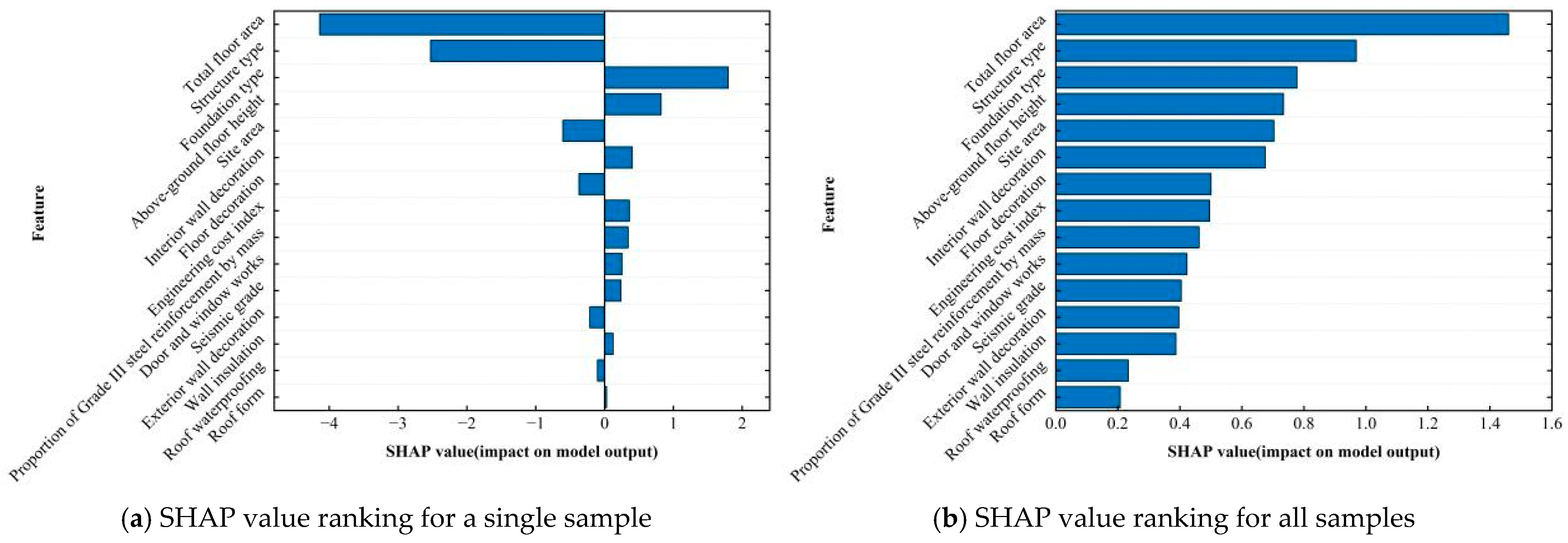
As the BP neural network is a ‘black-box model’ which only provides the input and output variables without indicating the importance of each input variable’s contribution to the output, this study uses SHAP to analyze the model’s interpretability. This approach can reveal which factors have the greatest impact on construction costs. As shown in Figure 13, subfigure (a) illustrates the SHAP value importance ranking for one sample. The greater the absolute SHAP value, the more influential the corresponding indicator is on the result, and vice versa. Subfigure (b) shows the ranking of the importance of SHAP values for all prediction samples, where the average absolute SHAP value of each indicator is shown. It can be seen that indicators such as total floor area and structure type have the greatest influence on construction costs, while indicators such as roof form and roof waterproofing have the least.

Figure 13. SHAP value ranking of each indicator.

7. Discussion

7.1. Predictive Performance and Significance of the Improved SSA-BP Model

The ISSA proposed in this study not only improves the optimization stability of SSA but also significantly enhances the fitting accuracy and generalization ability of the BP neural network in predicting the unit cost of residential buildings. This improvement can be attributed to the fact that Tent chaotic mapping enhances the spatial ergodicity of the initial population, while the dynamic adaptive weight enables the algorithm to maintain strong global search capability in the early stage and gradually shift toward refined local optimization in the later stage. As a result, more appropriate initial weights and thresholds can be provided for the BP network, thereby alleviating its tendency to fall into local optima and reducing fluctuations in training results. This finding is consistent with the results reported by An et al. [41]. The results of this study indicate that the standard BP model has difficulty fully capturing the complex nonlinear relationships among cost indicators, whereas the coupling of heuristic optimization algorithms with neural networks can improve prediction stability under small-sample conditions. This is consistent with the conclusions of Feng et al. [44]. The coupled model also provides practical benefits for cost management personnel. Traditional estimation methods usually rely on manual experience and comparisons with similar projects, resulting in relatively low efficiency [45]. In contrast, the ISSA-BP model can rapidly generate unit cost predictions after key engineering parameters are input, thereby improving estimation efficiency. During the investment decision-making and scheme design stages, engineering quantity information is often incomplete, and traditional methods are easily affected by subjective experience [46]. The proposed model can identify nonlinear relationships from historical data, thereby improving estimation accuracy and stability. Therefore, this study provides a new coupling strategy for improving BP neural networks using swarm intelligence optimization algorithms. It also offers a high-accuracy quantitative basis for early-stage investment decision-making, quota design, and cost deviation warning in residential building projects.

7.2. Engineering Mechanisms and Implications of Key Cost Drivers

The SHAP analysis results indicate that total floor area, structure type, and foundation type make relatively high contributions to the unit cost of residential buildings, reflecting the fundamental engineering logic underlying residential building cost formation. Total floor area directly determines the quantity basis of the main structure, envelope system, decoration works, installation works, and temporary measures. Variations in this indicator, therefore, simultaneously affect material consumption, labor input, mechanical equipment allocation, and construction organization costs. In this sense, total floor area essentially represents the scale effect of the project and the intensity of resource input. The importance of the structure type mainly arises from its comprehensive influence on the load-bearing system, component arrangement, material consumption, and construction techniques. Different structural systems vary in terms of steel reinforcement, concrete, formwork, scaffolding, seismic detailing measures, and construction difficulty, and may further affect the selection of the foundation form. Foundation type and site area reflect site conditions, load transfer paths, and the spatial extent of the foundation, thereby exerting a direct influence on earthwork, ground treatment, and foundation construction costs. Although indicators such as decoration works, door and window works, and the proportion of grade III steel reinforcement by mass are not the most influential factors, they respectively reflect building functional standards, the structure of material consumption, and market price fluctuations. These findings provide direct implications for engineering practice. During the investment estimation and scheme comparison stages, priority should be given to improving the accuracy of core parameters such as total floor area, structure type, foundation type, and major decoration standards. During the cost control stage, high-contribution indicators should be regarded as key review targets rather than allocating management resources evenly across all variables, thereby improving the precision and effectiveness of cost management. Similar studies have also indicated that explainable machine learning can identify key driving variables in engineering costs and enhance the usability of cost prediction results in practical decision-making [47,48].

7.3. Advantages and Limitations of the Coupled Model Framework

This study constructs a residential building cost prediction framework integrating algorithm improvement, indicator screening, model optimization, and result interpretation. Specifically, Tent chaotic mapping and a dynamic adaptive weight factor are introduced to improve the initial population randomization and global search capability of SSA. PCA is used to reduce indicator redundancy, ISSA is adopted to enhance the optimization of the initial weights and thresholds of the BP neural network, and SHAP is employed to reveal the key cost drivers and their engineering implications. Compared with studies that focus solely on improving prediction accuracy, the proposed framework not only enhances predictive performance but also facilitates the transformation from “black-box prediction” to “interpretable decision-making.” Wang et al. [49] also indicated that integrating machine learning prediction models with interpretability methods such as SHAP is an important direction for improving the transparency and practical application value of engineering cost prediction.

This study still has several limitations. First, the samples were mainly collected from residential building projects in Sichuan Province, which reflects relatively strong regional characteristics. However, labor prices, material prices, geological conditions, and local pricing rules may vary across different regions. Therefore, the applicability of the proposed model to other provinces or different types of buildings requires further verification. Second, the sample size used in this study is relatively limited. Although it is sufficient for model training, testing, and comparative analysis, the generalization ability of machine learning models is usually closely related to sample size, data quality, and feature completeness. Wang et al. [49] pointed out that this field still faces several challenges, such as insufficient dataset size, limited model applicability, and inadequate acquisition of engineering features. Therefore, future research could further expand the sample scope, establish a database covering multiple regions and different types of building projects, and incorporate external variables such as construction duration, project management level, and market price fluctuations. This would further verify the applicability and practical value of the model under different data scales and engineering scenarios.

8. Conclusions

This study aims to develop a residential building cost prediction method based on an improved SSA-optimized BP neural network, with consideration of prediction accuracy, model stability, and result interpretability. Through the performance testing of the ISSA algorithm, the comparison of nine prediction models, and SHAP analysis, the following conclusions are drawn:

(1)

The ISSA algorithm, together with GA, WPA, and SSA, was tested and compared using eight benchmark functions after Tent chaotic mapping and dynamic adaptive weights were incorporated to optimize the SSA algorithm. The results show that ISSA basically outperforms the other three algorithms in terms of convergence accuracy, stability, and convergence speed.

(2)

A residential building cost prediction model was established based on the BP neural network. The representative single-run results showed that the R2, RMSE, MAE, MAPE, and MBE values of the ISSA-BP model were 0.9754, 40.9194, 20.0025, 0.7633, and 11.9308, respectively, indicating that its overall performance was superior to those of BP, GA-BP, WPA-BP, and SSA-BP. Further validation was conducted through 30 independent runs with the inclusion of RF, ISSA-RF, XGBoost, and ISSA-XGBoost. The results showed that the mean R2, RMSE, MAE, MAPE, and MBE values of ISSA-BP were 0.9773, 39.2339, 17.0973, 0.6293, and 9.1583, respectively. These values were generally the best among the nine models, and the standard deviations of the five evaluation metrics were relatively small. The results indicate that ISSA-BP achieved the best overall performance among the nine prediction models.

(3)

The SHAP-based interpretability analysis revealed that the contributing factors influencing construction costs are, in descending order of importance: total floor area, structure type, foundation type, site area, interior wall decoration, floor decoration, engineering cost index, proportion of grade III steel reinforcement by mass, door and window works, seismic grade, exterior wall decoration, wall insulation, roof waterproofing, and roof form.

References

- Jia, Y.Z.; Yun, Z.C. Pose estimation method for construction machine based on improved AlphaPose model. Eng. Constr. Archit. Manag. 2024, 31, 976–996. [Google Scholar] [CrossRef] [Scilit]
- Jin, H.; Shen, L.; Wang, Z. Mapping the Influence of Project Management on Project Cost. KSCE J. Civ. Eng. 2018, 22, 3183–3195. [Google Scholar] [CrossRef] [Scilit]
- Chen, G.L.; Zheng, S.M.; He, X.R.; Liang, X.; Liao, X.H. Machine Learning-Based Cost Estimation Models for Office Buildings. Buildings 2025, 15, 1802. [Google Scholar] [CrossRef] [Scilit]
- Sargentis, G.F.; Defteraios, P.; Lagaros, N.D.; Mamassis, N. Values and Costs in History: A Case Study on Estimating the Cost of Hadrianic Aqueduct’s Construction. World 2022, 3, 260–286. [Google Scholar] [CrossRef] [Scilit]
- Walker, D.; Dart, J.C. Frontinus—A Project Manager from the Roman Empire Era. Proj. Manag. J. 2011, 42, 4–16. [Google Scholar] [CrossRef] [Scilit]
- Hashemi, T.S.; Ebadati, M.O.; Kaur, H. Cost estimation and prediction in construction projects: A systematic review on machine learning techniques. SN Appl. Sci. 2020, 2, 1703. [Google Scholar] [CrossRef] [Scilit]
- Li, C.Q.; Xiao, Y.; Xu, X.F.; Chen, Z.Y.; Zheng, H.F.; Zhang, H.L. Intelligent Forecast Model for Project Cost in Guangdong Province Based on GA-BP Neural Network. Buildings 2024, 14, 3668. [Google Scholar] [CrossRef] [Scilit]
- Zhang, Y.F.; Mo, H.J. Intelligent building construction cost optimization and prediction by integrating BIM and elman neural network. Heliyon 2024, 10, e37525. [Google Scholar] [CrossRef] [Scilit]
- Park, D.Y.; Yun, S.H. Construction Cost Prediction Using Deep Learning with BIM Properties in the Schematic Design Phase. Appl. Sci. 2023, 13, 7207. [Google Scholar] [CrossRef] [Scilit]
- Liu, Z.H.; Lin, J. Combinatorial machine learning approaches for high-rise building cost prediction and their interpretability analysis. J. Asian Archit. Build. Eng. 2025, 24, 2817–2828. [Google Scholar] [CrossRef] [Scilit]
- Han, K.; Wang, T.L.; Liu, W.H.; Li, C.S.; Xian, X.C.; Yang, Y.Y. Construction cost prediction model for agricultural water conservancy engineering based on BIM and neural network. Sci. Rep. 2025, 15, 24271. [Google Scholar] [CrossRef] [Scilit]
- Hirijanto; Mundra, I.W.; Utomo, A. Cost prediction model based on system dynamics in water resource project. MATEC Web Conf. 2019, 258, 02027. [Google Scholar] [CrossRef] [Scilit]
- Li, X.N.; Han, K.; Liu, W.H.; Wang, T.L.; Li, C.H.; Yan, B.; Hao, C.M.; Xian, X.C.; Yang, Y.Y. Prediction Model of Farmland Water Conservancy Project Cost Index Based on PCA–DBO–SVR. Sustainability 2025, 17, 2702. [Google Scholar] [CrossRef] [Scilit]
- Simić, N.; Ivanišević, N.; Nedeljković, Đ.; Senić, A.; Stojadinović, Z.; Ivanović, M. Early Highway Construction Cost Estimation: Selection of Key Cost Drivers. Sustainability 2023, 15, 5584. [Google Scholar] [CrossRef] [Scilit]
- Tijanić, K.; Car-Pušić, D.; Šperac, M. Cost estimation in road construction using artificial neural network. Neural Comput. Appl. 2019, 32, 9343–9355. [Google Scholar] [CrossRef] [Scilit]
- Lu, Y.; Niu, D.X.; Qiu, J.P.; Liu, W.D. Prediction Technology of Power Transmission and Transformation Project Cost Based on the Decomposition-Integration. Math. Probl. Eng. 2015, 2015, 651878. [Google Scholar] [CrossRef] [Scilit]
- Ma, L.; Wang, Q.X.; Liao, S.; Guo, T.; Xiong, Y.; Ming, Y.; Zou, Y.X. Research on Cost Prediction of Power Transmission and Transformation Project Based on Combination Prediction Model. IOP Conf. Ser. Earth Environ. Sci. 2021, 769, 042019. [Google Scholar] [CrossRef] [Scilit]
- Kovačević, M.; Ivanišević, N.; Petronijević, P.; Despotović, V. Construction cost estimation of reinforced and prestressed concrete bridges using machine learning. Građevinar 2021, 73, 1–13. [Google Scholar] [CrossRef] [Scilit]
- Fernando, N.; Kasun, D.; Zhang, H. An artificial neural network (ANN) approach for early cost estimation of concrete bridge systems in developing countries: The case of Sri Lanka. J. Financ. Manag. Prop. Constr. 2024, 29, 23–51. [Google Scholar] [CrossRef] [Scilit]
- Marco, D.A.; Ottaviani, M.F.; Bolognesi, F. Time series-based Project Cost Forecasting Framework. Procedia Comput. Sci. 2024, 239, 102–113. [Google Scholar] [CrossRef] [Scilit]
- Elfahham, Y. Estimation and prediction of construction cost index using neural networks, time series, and regression. Alex. Eng. J. 2019, 58, 499–506. [Google Scholar] [CrossRef] [Scilit]
- Dharwadkar, V.N.; Arage, S.S. Prediction and estimation of civil construction cost using linear regression and neural network. Int. J. Intell. Syst. Des. Comput. 2018, 2, 28–44. [Google Scholar] [CrossRef] [Scilit]
- Antoniou, F.; Aretoulis, G.; Giannoulakis, D.; Konstantinidis, D. Cost and Material Quantities Prediction Models for the Construction of Underground Metro Stations. Buildings 2023, 13, 382. [Google Scholar] [CrossRef] [Scilit]
- Salahaldain, Z.; Naimi, S.; Alsultani, R. Estimation and Analysis of Building Costs Using Artificial Intelligence Support Vector Machine. Math. Model. Eng. Probl. 2023, 10, 405–411. [Google Scholar] [CrossRef] [Scilit]
- Michał, J. Development of Cost Estimation Models Based on ANN Ensembles and the SVM Method. Civ. Environ. Eng. Rep. 2020, 30, 48–67. [Google Scholar] [CrossRef] [Scilit]
- Juszczyk, M. On the Search of Models for Early Cost Estimates of Bridges: An SVM-Based Approach. Buildings 2019, 10, 2. [Google Scholar] [CrossRef] [Scilit]
- Jiang, Q.H. Estimation of construction project building cost by back-propagation neural network. J. Eng. Des. Technol. 2020, 18, 601–609. [Google Scholar] [CrossRef] [Scilit]
- Chen, L.J.; Wang, D.J. Cost Estimation and Prediction for Residential Projects Based on Grey Relational Analysis–Lasso Regression–Backpropagation Neural Network. Information 2024, 15, 502. [Google Scholar] [CrossRef] [Scilit]
- Wang, R.; Salleh, H.; Li, K.Y.; Abdul Samad, Z. A conceptual cost estimation model for building construction projects by hybrid Back-Propagation Neural Network and Dung Beetle Optimizer algorithm. J. Asian Archit. Build. Eng. 2025, 24, 5520–5542. [Google Scholar] [CrossRef] [Scilit]
- Lowe, D.J.; Emsley, M.W.; Harding, A. Predicting construction cost using multiple regression techniques. J. Constr. Eng. Manag. 2006, 132, 750–758. [Google Scholar] [CrossRef] [Scilit]
- Choi, C.Y.; Ryu, K.R.; Shahandashti, M. Predicting city-level construction cost index using linear forecasting models. J. Constr. Eng. Manag. 2021, 147, 04020158. [Google Scholar] [CrossRef] [Scilit]
- Petruseva, S.; Zileska-Pancovska, V.; Žujo, V.; Brkan-Vejzović, A. Construction costs forecasting: Comparison of the accuracy of linear regression and support vector machine models. Tech. Gaz. 2017, 24, 1431–1438. [Google Scholar] [CrossRef] [Scilit]
- Li, L. Dynamic Cost Estimation of Reconstruction Project Based on Particle Swarm Optimization Algorithm. Informatica 2023, 47, 173–182. [Google Scholar] [CrossRef] [Scilit]
- Xu, X.M.; Peng, L.Y.; Ji, Z.S.; Zheng, S.P.; Tian, Z.X.; Geng, S.P. Research on Substation Project Cost Prediction Based on Sparrow Search Algorithm Optimized BP Neural Network. Sustainability 2021, 13, 13746. [Google Scholar] [CrossRef] [Scilit]
- Wu, Y.; Lan, S.; Liu, T.T. Research on engineering cost prediction based on GA-BP neural network. Int. J. Bus. Intell. Data Min. 2025, 26, 362–381. [Google Scholar] [CrossRef] [Scilit]
- Wang, Y.; Shi, Y.; Yang, T.Y.; Wang, W.N.; Sun, Z.M.; Zhang, Y.Q. Structural Performance Warning Based on Computer Intelligent Monitoring and Fractional-Order Multi-Rate Kalman Fusion Method. Fractal Fract. 2026, 10, 186. [Google Scholar] [CrossRef] [Scilit]
- Wu, X.Y.; Wang, Z.W.; Duan, H.X.; Gan, Y.X.; Chen, S.H.; Li, M.; Zhao, X.; Xu, E.P. Settlement Prediction of Preloading Method Based on SSA-BP Neural Network with Consideration of Asymmetric Settlement Behavior. Symmetry 2025, 17, 1989. [Google Scholar] [CrossRef] [Scilit]
- Zhou, Y.X.; Shi, J.G.; Han, X.Y.; Kong, X.P.; Liu, Y.J.; Ren, Y.N.; Zeng, J.Y. Research on the Prediction of Blasting Vibration Velocity in Open Pit Mines Based on the SSA-BP Model. ACS Omega 2025, 10, 57315–57334. [Google Scholar] [CrossRef] [Scilit]
- Xue, J.K.; Shen, B. A novel swarm intelligence optimization approach: Sparrow search algorithm. Syst. Sci. Control Eng. 2020, 8, 22–34. [Google Scholar] [CrossRef] [Scilit]
- Geng, J.Q.; Meng, W.G.; Yang, Q.R. Electricity Substitution Potential Prediction Based on Tent-CSO-CG-SSA-Improved SVM—A Case Study of China. Sustainability 2022, 14, 853. [Google Scholar] [CrossRef] [Scilit]
- An, X.Y.; Wang, H.Y.; Shi, B.J.; Zhang, J.; Ren, C.L.; Mei, Y.X. Temperature Compensation of Infrared Gas Sensor Based on ISSA-BP Algorithm. Infrared Technol. 2025, 47, 1296–1304. Available online: http://hwjs.nvir.cn/en/article/id/d9d59b04-9034-491a-8815-cc01b9e874e5 (accessed on 15 January 2026).
- Yan, H.Y.; He, Z.; Gao, C.; Xie, M.J.; Sheng, H.Y.; Chen, H.H. Investment estimation of prefabricated concrete buildings based on XGBoost machine learning algorithm. Adv. Eng. Inform. 2022, 54, 101789. [Google Scholar] [CrossRef] [Scilit]
- Asgarkhani, N.; Kazemi, F.; Jankowski, R.; Formisano, A. Dynamic ensemble-learning model for seismic risk assessment of masonry infilled steel structures incorporating soil-foundation-structure interaction. Reliab. Eng. Syst. Saf. 2026, 267, 111839. [Google Scholar] [CrossRef] [Scilit]
- Feng, R.; Liu, W. LSSA-BP-based cost forecasting for onshore wind power. Energy Rep. 2023, 9, 362–370. [Google Scholar] [CrossRef] [Scilit]
- Habib, O.; Abouhamad, M.; Bayoumi, A. Ensemble learning framework for forecasting construction costs. Autom. Constr. 2024, 170, 105903. [Google Scholar] [CrossRef] [Scilit]
- Lee, J.G.; Lee, H.S.; Park, M.; Seo, J. Early-stage cost estimation model for power generation project with limited historical data. Eng. Constr. Archit. Manag. 2022, 29, 2599–2614. [Google Scholar] [CrossRef] [Scilit]
- Meng, C.; Qu, D.; Duan, X. Cost Estimation of Metro Construction Projects Using Interpretable Machine Learning. J. Comput. Civ. Eng. 2024, 38, 04024038. [Google Scholar] [CrossRef] [Scilit]
- Larocque, R.; Boulé, A.M.; Cappart, Q. Estimating Road Construction Costs with Explainable Machine Learning. INFORMS J. Appl. Anal. 2025, 55, 137–153. [Google Scholar] [CrossRef] [Scilit]
- Wang, R.; Salleh, H.; Lyu, J.; Abdul-Samad, Z.; Radzuan, N.F.M.; Wen, K.C. Application and prospect of machine learning techniques in cost estimation of building projects. Eng. Constr. Archit. Manag. 2025, 32, 8445–8471. [Google Scholar] [CrossRef] [Scilit]
Disclaimer/Publisher’s Note: The statements, opinions and data contained in all publications are solely those of the individual author(s) and contributor(s) and not of MDPI and/or the editor(s). MDPI and/or the editor(s) disclaim responsibility for any injury to people or property resulting from any ideas, methods, instructions or products referred to in the content. |
© 2026 by the authors. Licensee MDPI, Basel, Switzerland. This article is an open access article distributed under the terms and conditions of the Creative Commons Attribution (CC BY) license.