Sequential Visual–Spatial States and Visitor Behavior in a Linear Green Waterfront Corridor: Evidence from the Grand Canal, Beijing

Abstract

Linear green waterfront corridors are important public open spaces where movement, spatial experience, and recreational behavior unfold continuously along paths. However, the visual–spatial conditions associated with visitor behavior in such settings remain insufficiently understood, particularly from the perspective of sequential spatial experience. Using the Tongzhou section of the Grand Canal in Beijing as a case study, this study examined how visitor movement and staying rhythms vary across visual–spatial environments along a linear corridor. Sixteen visual–spatial indicators were derived from 1505 georeferenced panoramic images, and approximately 1.65 million GPS trajectory points were used as external behavioral evidence. Five latent visual–spatial states were identified along the corridor sequence, and the contributions of different indicators to state differentiation were further interpreted. The results show that the corridor was organized into differentiated visual–spatial states with clear continuity and gradual transitions, and that visitor behavior differed significantly across these states. High visit intensity did not necessarily correspond to a high stay ratio, and lower movement speed did not uniformly indicate stopping. The strongest state-differentiation signals were associated with depth-informed structural variables, especially the closely related foreground proportion and average depth, together with waterfront-interface conditions. These findings extend current understanding of visual–spatial environment–behavior relationships in linear public green spaces and provide methodological support for the planning, design, and management of waterfront and other linear public green environments.

1. Introduction

Linear green waterfront corridors are key components of urban green infrastructure and major settings for everyday recreation [1], environmental experience [2], and human–nature interaction [3]. Such corridors serve as accessible interfaces between residents and urban waters, facilitating physical activity and mental restoration with broader benefits for public health, and are also closely associated with urban public vitality [4,5,6]. How people perceive and use such environments is often shaped by multiple human dimensions, including naturalness, aesthetics, safety, and access [7]. Unlike independent parks or plazas, linear green waterfront corridors are primarily experienced through movement, as visitors continuously encounter changing vegetation interfaces, waterfront edges, sightlines, and spatial depths along the route [8,9]. Therefore, understanding how visual–spatial conditions are sequentially organized at the pedestrian scale is important for the design and management of waterfront public spaces.

In this context, research on visitor behavior in urban open spaces has gradually shifted from simple flow measurement toward closer examination of the relationships between environmental perception and human activity [10,11]. Increasing attention has been paid to staying behavior [12], movement patterns [13], and the influence of the built and natural environment on everyday spatial practices [14,15]. This shift has also created new opportunities to relate observed trajectories to experienced environments.

Environmental psychology posits that spatial experience is grounded in visual perception, with human behavior in outdoor settings shaped by visual–spatial cues, particularly those related to prospect–refuge conditions [16,17] and the preference matrix framework [18,19]. Recent studies have translated these ideas into measurable indicators from the pedestrian perspective, including visibility-based measures, green view index, sky view factor, and enclosure-related proxies [20,21,22]. Empirical studies at larger scales have linked these visual attributes to emotional responses, health outcomes, and broader socio-spatial variations in cities [23,24,25,26]. Existing research has primarily examined green and waterfront environments through visual composition, perceived quality, and semantic content [27,28,29]. While these approaches have advanced the quantitative study of visual environments, they largely represent scenes as two-dimensional compositions, with limited consideration of human-scale three-dimensional spatial structure.

This limitation is more critical in linear corridors, where spatial experience unfolds as a sequence and is shaped by both visible content and depth-based spatial organization. Depth, enclosure, continuity, and the rhythm of spatial transition reflect the morphology of experienced space rather than surface appearance alone [30,31,32]. Yet it remains unclear how such environments are organized as sequential experiences, how depth-informed structure differentiates corridor settings, and how this differentiation relates to visitor behavior. In corridor environments, experience is formed through a continuous sequence of changing interfaces and spatial states rather than through isolated views [33,34,35].

Recent advances in computer vision provide useful tools for addressing this gap. Semantic segmentation enables the extraction of environmental content from images, while monocular depth estimation provides pixel-level depth cues that can be translated into structural properties relevant to openness, enclosure, and depth gradients [14,36,37,38]. At the same time, Hidden Markov Models (HMMs) offer a suitable way to identify latent sequential patterns embedded in ordered observations [39,40,41]. However, existing studies have rarely integrated image-derived structural indicators, latent state identification, and externally observed visitor behavior within a unified framework to examine sequential visual–spatial experience in linear waterfront public spaces.

Against this backdrop, this study focuses on a linear green waterfront corridor and uses the Tongzhou section of the Grand Canal in Beijing as a case study. By integrating panoramic image analysis with GPS trajectory data, this study derives visual–spatial indicators from panoramic images, identifies latent states along the sequential path, and uses trajectories as external behavioral evidence to examine how visitors’ movement and staying rhythms vary across visual–spatial environments [42]. Accordingly, this study addresses two questions: what recognizable visual–spatial states emerge along visitors’ movement paths in a linear green waterfront corridor, and how are visitor movement and staying behaviors distributed across these states? By integrating depth-informed spatial structure, environmental content, and behavioral evidence within a unified framework, this study advances understanding of how experienced environments are associated with visitor behavior in linear waterfront public spaces and provides methodological support for the design and management of waterfront and other linear public settings.

2. Study Area and Data

2.1. Study Area

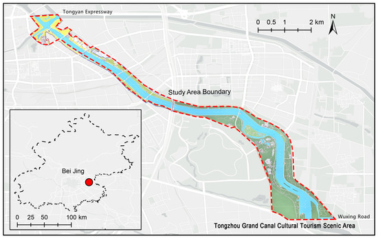
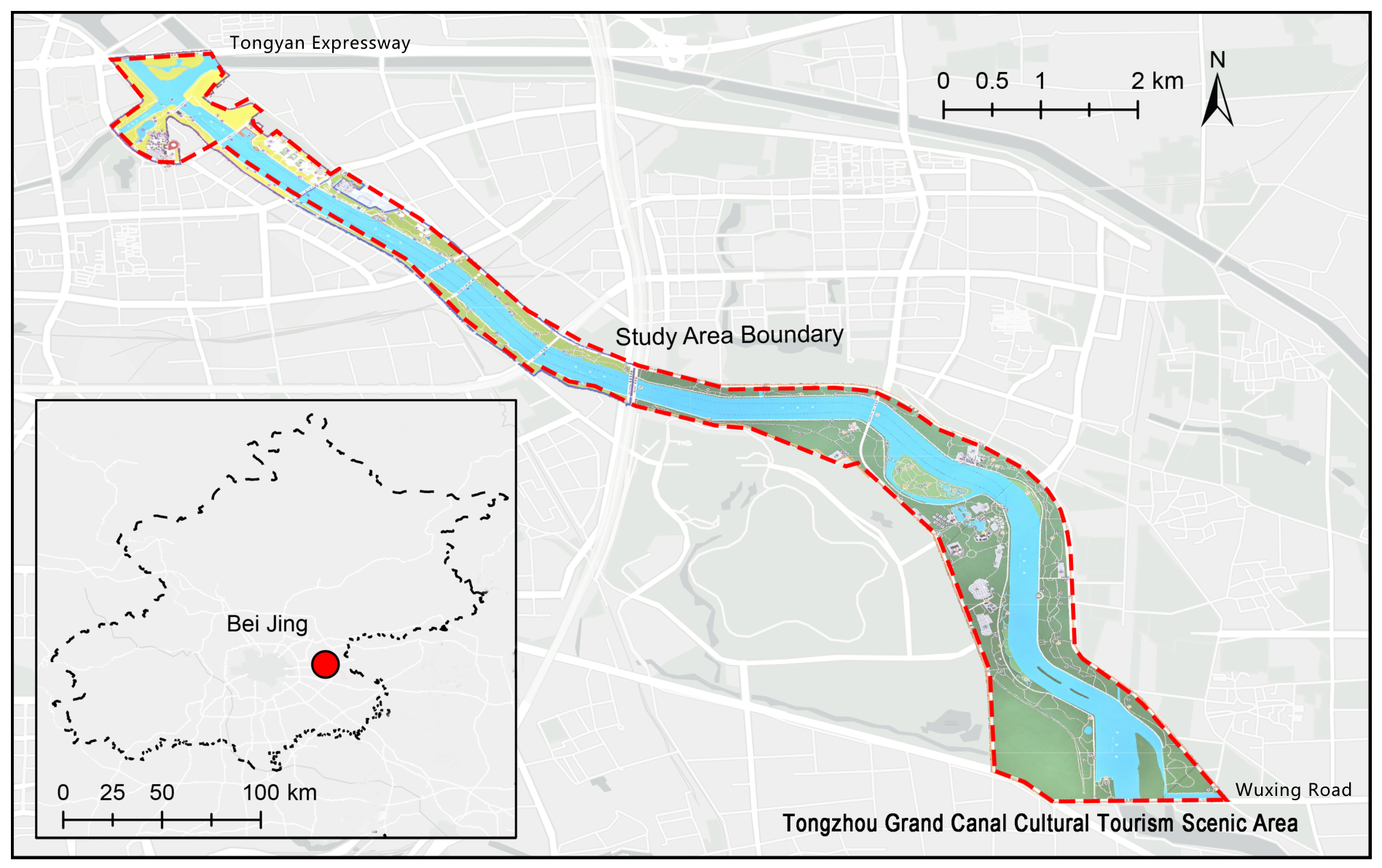
This study selected the Tongzhou section of the Grand Canal Cultural Tourism Area, located in southeastern Beijing, as the study site (Figure 1). This area constitutes an important part of the Beijing section of the Grand Canal. The canal section is approximately 12.1 km long and covers a total area of about 7.23 km², of which 2.56 km² is water surface. The study section starts at Tongyan Expressway in the north and ends at Wuxing Road in the south. Historically, the Tongzhou section served as a key hub for north–south grain transportation and preserves rich canal heritage, making it an important witness to the cultural history of the Grand Canal [43]. In recent years, a series of ecological restoration and landscape enhancement projects have been implemented along the canal in Tongzhou, forming a waterfront cultural space network structured by green corridors, cultural nodes, and public activity spaces [44]. With its continuous waterfront walking corridor and diverse spatial interfaces, the area presents a strongly sequential linear landscape environment, providing an ideal setting for examining the relationship between visual–spatial experience and visitor behavior along a movement path.

2.2. Panoramic Images

Panoramic images along the canal corridor were collected in May 2025 using an Insta360 panoramic camera mounted on a mobile carrier along the main pathways. All images were georeferenced using synchronized GPS records. To ensure spatial representativeness and a relatively uniform sampling density, image frames were retained at an interval threshold of approximately 20 m (±2 m). The lower 25% of each image was removed, and all retained images were standardized to a consistent format, resulting in a final dataset of 1505 high-quality georeferenced panoramic images.

2.3. GPS Trajectory Data

Visitor trajectories were obtained from the Chinese outdoor activity platform 2bulu, which provides geographic records with timestamps and route information. As 2bulu is a voluntary outdoor activity recording platform, the trajectory records are more likely to reflect users who actively record outdoor routes. Therefore, these data are used as platform-recorded behavioral traces to examine relative spatial differences in movement and potential staying across corridor segments. Previous research has shown that 2bulu trajectory data can reliably reflect actual travel routes in case-study settings [45]. The raw trajectory records used in this study span from April 2012 to December 2025. They were preprocessed through spatial filtering and temporal cleaning to retain valid trajectories overlapping with the study area and to remove records with abnormal time intervals, resulting in a final dataset of approximately 1.65 million valid trajectory points.

3. Methods

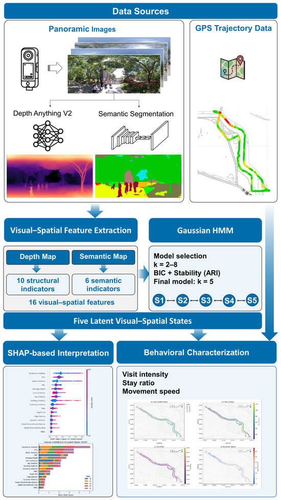
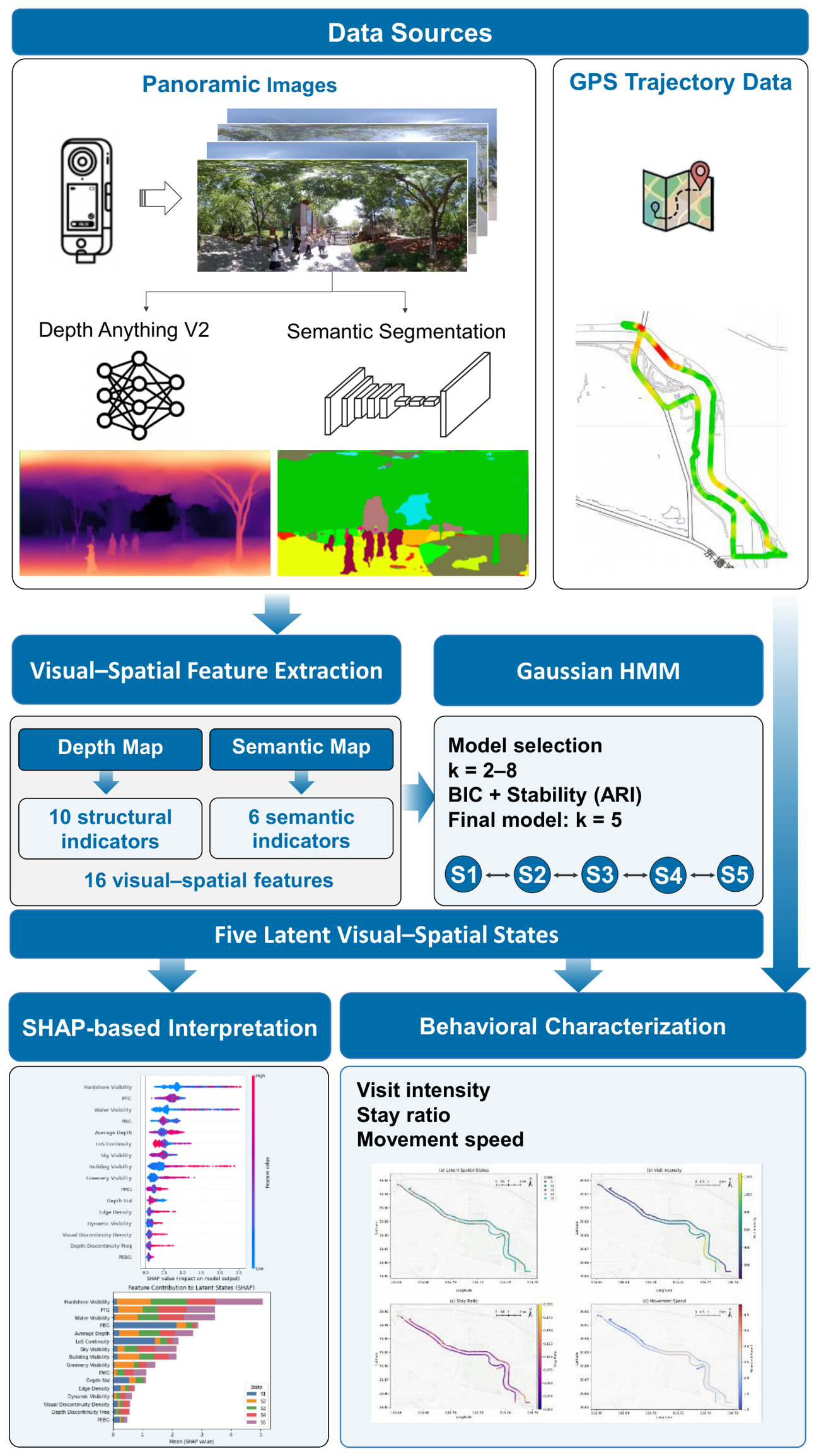
The methodological workflow of this study is shown in Figure 2, which illustrates how panoramic images and GPS trajectories were processed and linked to identify latent visual–spatial states and interpret their behavioral differences.

3.1. Quantification of Visual–Spatial

3.1.1. Monocular Depth Estimation

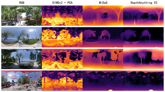
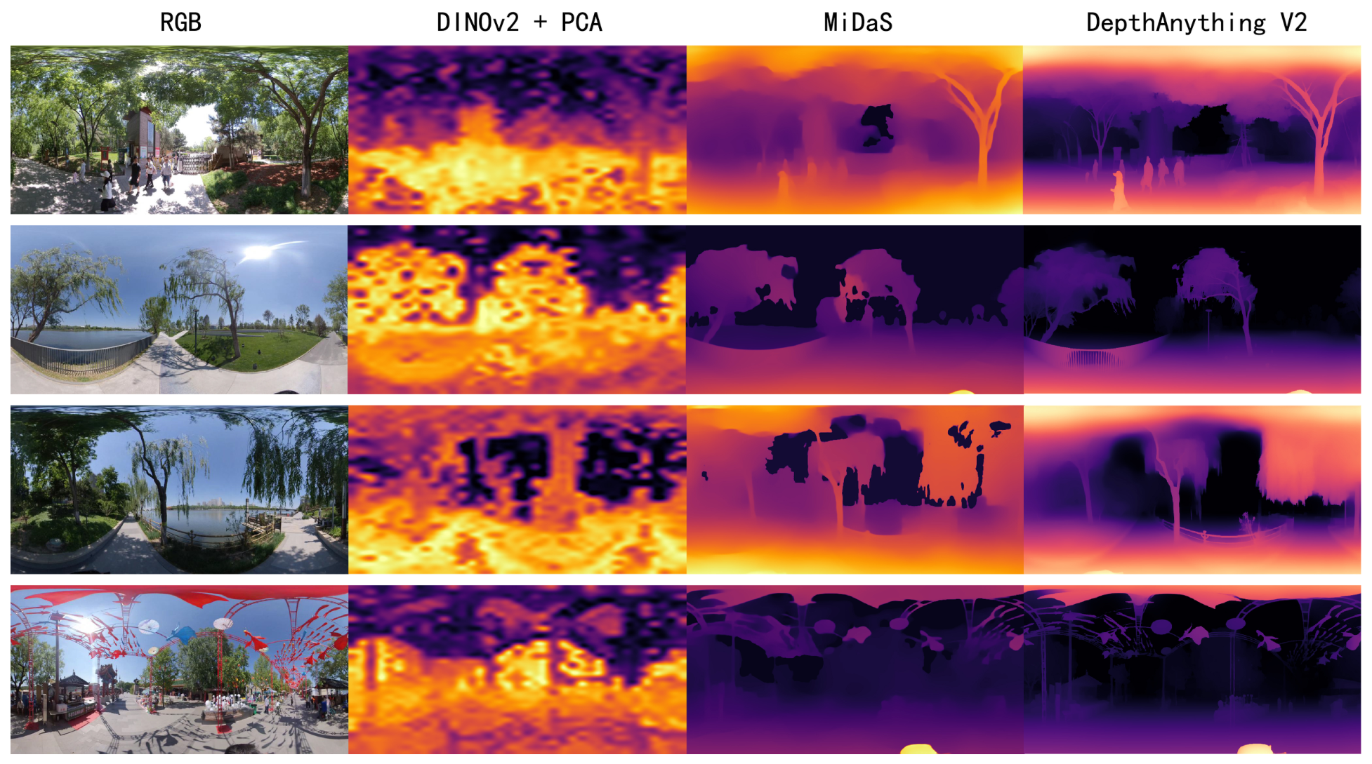
Monocular depth was estimated using Depth Anything V2. The selection of this model was based on a qualitative comparative analysis of representative samples, where its visual superiority was evident in maintaining depth gradient continuity and boundary stability. Preliminary comparison with MiDaS and DINOv2 + PCA (Figure 3) indicated that Depth Anything V2 produced smoother depth transitions and more stable spatial layering, particularly in challenging scenes containing water reflections, dense vegetation, and mixed boundary conditions. These qualitative improvements in robustness and structural consistency were the primary basis for its adoption in this study.

Before inference, all images were standardized using Z-score normalization. The model combines a Transformer-based backbone with feature-pyramid fusion to encode multiscale image information and generate a single-channel 8-bit depth map for each image. These depth maps were then used to derive indicators of spatial layering, openness, enclosure, and visual continuity.

3.1.2. Structural Indicators of Visual–Spatial Organization

Based on the 8-bit grayscale depth maps (0–255), 10 structural indicators were constructed to describe three aspects of spatial organization: spatial layering, depth statistics, and structural continuity.

To represent the hierarchical composition of visual depth, each depth map was divided into four depth bands using fixed grayscale intervals: foreground proportion (PFG, 0–64), midground proportion (PMG, 65–128), background proportion (PBG, 129–192), and far-background proportion (PEBG, 193–255) [26]. The proportion of each band was calculated as follows:

$$PFG={\displaystyle \frac{1}{N}}{\displaystyle \sum _{i=1}^N{1}_{\{d_i\le 64\}}}\times 100\%$$

(1)

$$PMG={\displaystyle \frac{1}{N}}{\displaystyle \sum _{i=1}^N{1}_{\{65\le d_i\le 128\}}}\times 100\%$$

(2)

$$PBG={\displaystyle \frac{1}{N}}{\displaystyle \sum _{i=1}^N{1}_{\{129\le d_i\le 192\}}}\times 100\%$$

(3)

$$PEBG={\displaystyle \frac{1}{N}}{\displaystyle \sum _{i=1}^N{1}_{\{d_i>192\}}}\times 100\%$$

(4)

Two additional indicators, Average Depth and Depth Std, were used to summarize overall depth characteristics. Average Depth represents the general viewing distance and openness of the scene, whereas Depth Std reflects internal depth variation and thus the heterogeneity of spatial layering.

$$\overline{d}={\displaystyle \frac{1}{N}}{\displaystyle \sum _{i=1}^N{d}_i}$$

(5)

$${\sigma }_d=\sqrt{{\displaystyle \frac{1}{N}}{\displaystyle \sum _{i=1}^N{(d_i-\overline{d})}^2}}$$

(6)

To capture structural continuity and geometric complexity, four further indicators were derived from the depth maps: Edge Density, Depth Discontinuity Freq, LoS Continuity, and Visual Discontinuity Density. Together, these indicators describe the extent to which space unfolds smoothly or appears fragmented at the pedestrian scale.

3.1.3. Semantic Segmentation of Environmental Content

Because depth estimation captures spatial structure but not environmental content, semantic segmentation was further applied to all panoramic images. This step was conducted using the semantic-segmentation-pytorch toolbox developed by MIT CSAIL (https://github.com/CSAILVision/semantic-segmentation-pytorch, accessed on 2 April 2026), with a ResNet101–UPerNet model pretrained on the ADE20K dataset for pixel-level recognition [46]. The pretrained ADE20K model was used to derive approximate environmental-content measures at a large sample scale. However, because the model was not specifically trained on Chinese waterfront corridor environments, the aggregated semantic indicators were interpreted as comparative scene-content measures rather than as pixel-level ground-truth classifications.

The model combines a convolutional backbone and a multiscale decoding module to generate stable semantic predictions across 150 scene categories. The segmentation outputs were then converted into RGB masks and used for the extraction of interpretable environmental-content indicators.

3.1.4. Extraction of Environmental Content Indicators

To quantify environmental content, the original ADE20K labels were grouped into six aggregated environmental categories: building, greenery, sky, water, hard shore, and dynamic elements (

Table 1. Aggregated environmental categories and their corresponding ADE20K labels used for semantic segmentation.

Category Identifier	Includes Subcategories (ADE20K Original Category Names)	Category IDs
Building Visibility	building, house, skyscraper, tower, castle, hut, garage, church, temple, cathedral	[10, 31, 32, 34, 65, 117, 136, 137, 138, 139]
Greenery Visibility	tree, grass, field, plant, flower, hedge, potted plant	[20, 21, 51, 123, 130, 143, 144]
Water Visibility	river, sea, waterfall, swimming pool, lake, water	[97, 49, 50, 60, 125, 129]
Sky Visibility	sky, cloud	[2, 106]
Hard shore Visibility	wall, fence, railing, bridge	[82, 83, 84, 38]
Dynamic Visibility	person, rider, car, bus, truck, train, motorcycle, bicycle	[11, 12, 13, 22, 23, 24, 25, 26, 27]

). This aggregation was based on the official ADE20K definitions and on functional distinctions commonly used in urban landscape analysis.

For each image, the visibility proportion of each category was calculated as the ratio of pixels belonging to the corresponding label set to the total number of pixels in the image. These six indicators describe the relative prominence of key environmental components in the visual field. Together with the ten structural indicators, these six semantic indicators formed a 16-dimensional visual–spatial feature set for subsequent modeling.

$${\mathrm{Visibility}}_c={\displaystyle \frac{1}{H\times W}}{\displaystyle \sum _{i=1}^{H\times W}{1}_{\{l_i\in {\mathcal{L}}_c\}}}\times 100\%$$

(7)

3.2. Behavioral Characterization from GPS Trajectories

Based on the preprocessed trajectory dataset, visitor behavior was further characterized by spatially linking trajectory records to the decoded visual–spatial states. Each trajectory consisted of sequential point records containing a track identifier, longitude, latitude, timestamp, and speed. These records provided the basis for deriving state-related behavioral indicators.

To establish the relationship between behavior and visual–spatial conditions, a 20 m buffer was generated around each image sampling location. This buffer size was selected to align with the image sampling interval and ensure spatial matching precision. Trajectory points falling within each buffer were assigned to the corresponding sampling location and its decoded latent state. Based on this matching procedure, three state-level behavioral indicators were constructed: visit intensity, stay ratio, and movement speed.

Visit intensity was defined as the number of trajectory points falling within the 20 m buffer of each sampling location, representing the spatial concentration of visitor activity. Because this point-based measure may be affected by recording frequency, trajectory duration, and repeated records from the same user, it was interpreted as the relative spatial concentration of platform-recorded activity rather than as the absolute number of visitors. Stay points were identified using a speed threshold, with trajectory points slower than 0.5 m/s classified as potential staying points to distinguish localized staying from slow movement. The 0.5 m/s threshold was selected as a conservative operational criterion because it is substantially lower than typical walking speed; therefore, points below this threshold were interpreted as potential staying or near-stationary points rather than directly observed stationary behavior, especially given that the platform trajectories may include mixed activities such as walking, cycling, and running. Stay ratio was then calculated as the proportion of staying points among all matched trajectory points at each sampling location. Movement speed was represented by the speed values recorded in the matched trajectory points and was aggregated to characterize the pace of movement across different corridor segments.

After calculation at the sampling-point level, these behavioral indicators were further aggregated at the latent-state level to support comparisons of visitor behavior across the identified visual–spatial states. Geographic Information Systems (GIS) were used throughout this stage to ensure consistent spatial alignment, aggregation, and visualization.

3.3. HMM-Based Identification of Latent Visual–Spatial States

A Gaussian HMM was used to identify latent visual–spatial states from sequentially ordered image samples along the linear corridor. Each observation corresponded to one image sampling location and was represented by a 16-dimensional visual–spatial feature vector derived from the structural and semantic indicators. Before model fitting, all features were standardized to ensure comparability across variables. The HMM assumes that the observed feature vectors are generated by a finite set of latent states, each characterized by a multivariate Gaussian distribution. By modeling transitions between adjacent observations, the HMM preserves sequential continuity along the corridor and partitions the visual environment into discrete but internally related visual–spatial states.

The number of latent states was determined by jointly considering model fit and stability. Candidate models with different state numbers were compared using the Bayesian Information Criterion (BIC), and clustering consistency across repeated random initializations was evaluated using the Adjusted Rand Index (ARI). This combined criterion was used to balance parsimony and robustness in state selection.

Model parameters were estimated using the Expectation–Maximization (EM) algorithm. After training, the Viterbi algorithm was applied to decode the most probable latent-state sequence for all image sampling locations. The decoded states were then mapped back to geographic space for subsequent analyses of spatial distribution, transition patterns, and state-related behavioral differences.

3.4. Post Hoc Interpretation of State Differentiation Using SHAP

To interpret how the 16 visual–spatial indicators contributed to the differentiation of the latent states identified by the HMM, this study employed SHapley Additive exPlanations (SHAP) as a post hoc interpretive approach [47]. Since the Gaussian HMM does not directly provide feature contribution scores, we utilized KernelSHAP, a model-agnostic method that treats the HMM as a functional mapping. This approach estimates SHAP values by observing changes in the posterior probabilities of each state in response to systematic perturbations of the 16 structural and semantic variables.

Based on this framework, SHAP values were computed to estimate the marginal contribution of each indicator to the prediction of each state. This enabled a quantitative comparison of the relative importance of depth-informed structural variables and environmental-content indicators in contributing to model-based state separation. To facilitate cross-state interpretation, SHAP results were further aggregated at the state level to identify the dominant features associated with each latent visual–spatial state. These findings provided a robust evidence base for the subsequent characterization of corridor state types and the analysis of their behavioral implications.

4. Results

4.1. Distribution Characteristics of Visual Indicators in Panoramic Images

4.1.1. Visual–Spatial Characteristics of Panoramic Images

The panoramic images showed substantial variation across both structural and semantic indicators, indicating marked heterogeneity in the visual–spatial environment of the corridor (

Table 2. Descriptive statistics of the 16 visual–spatial indicators for the 1505 sampled locations.

Indicator	Mean	Std. Dev.	Min	Max	Median
Average Depth	55.147	22.581	14.4	110.95	53.13
Depth Std	51.998	14.113	22.5	78.03	56.78
PFG	63.878	16.674	17.07	99.43	64.99
PMG	23.762	9.958	0.12	66.62	22.91
PBG	8.436	6.618	0.03	30.94	8.64
PEBG	3.923	3.63	0.02	17.77	4.02
Edge Density	0.557	0.35	0.03	2.96	0.51
Depth Discontinuity Freq	2.294	1.11	0.05	8.86	2.14
LoS Continuity	0.745	0.244	0.17	1	0.76
Visual Discontinuity Density	7.723	4.239	0.02	36.06	7.11
Building Visibility	0.73	1.455	0.04	14.62	0.25
Greenery Visibility	4.915	6.428	0.02	37.26	2.52
Sky Visibility	32.652	14.549	0.03	57.15	34.09
Hardshore Visibility	0.175	0.502	0.03	5.24	0.02
Dynamic Visibility	7.845	7.847	0.02	35.08	5.31
Water Visibility	0.092	0.338	0.05	5.11	0.03

N = 1505.

). In terms of structural indicators, Average Depth had a mean of 55.147 (SD = 22.581; range = 14.40–110.95), while Depth Std averaged 51.998. In the depth-layering structure, PFG had the highest mean value (63.878%), followed by PMG (23.762%), whereas PBG (8.436%) and PEBG (3.923%) were much lower. Among the continuity-related indicators, Edge Density averaged 0.557 and LoS Continuity 0.745, while Visual Discontinuity Density showed relatively large variation (mean = 7.723, SD = 4.239).

In terms of semantic indicators, Sky Visibility had the highest mean value (32.652%), followed by Dynamic Visibility (7.845%) and Greenery Visibility (4.915%), both of which also showed relatively large standard deviations. By contrast, Building Visibility (0.730%), Hardshore Visibility (0.175%), and Water Visibility (0.092%) remained low overall. Taken together, these results indicate that the corridor was characterized by a foreground-dominant depth structure, relatively continuous sightlines, and unevenly distributed semantic content.

4.1.2. Pearson Correlation Analysis of Visual Indicators

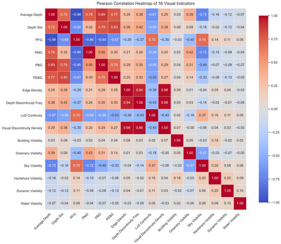
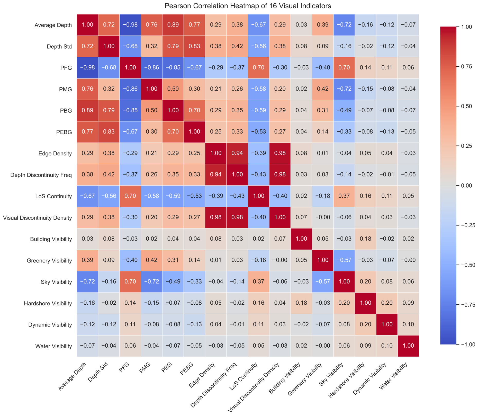
The Pearson correlation results among the 16 visual indicators are shown in Figure 4. Overall, no pervasive high-correlation pattern was observed. The mean absolute off-diagonal correlation coefficient was approximately 0.28, indicating generally low to moderate associations and limited overall redundancy among the indicators. This suggests that the structural and semantic variables captured complementary aspects of the corridor’s visual–spatial environment.

Among the specific relationships, PFG showed an extremely strong negative correlation with Average Depth (r = −0.98), indicating that scenes with a larger foreground proportion tended to have shallower overall perceived depth. Sky Visibility was moderately negatively correlated with both Greenery Visibility (r = −0.57) and PBG (r = −0.49), suggesting that greater sky exposure was generally associated with reduced vegetation visibility and weaker background layering. In addition, Edge Density showed an extremely strong positive correlation with Visual Discontinuity Density (r = 0.98), indicating a close association between richer boundary structure and stronger visual fragmentation.

4.2. HMM Results

4.2.1. Model Construction and Determination of the Number of States

A diagonal covariance matrix was adopted to improve the stability and efficiency of parameter estimation. Model training was performed using the Expectation–Maximization (EM) algorithm, with a maximum of 2000 iterations and a log-likelihood convergence threshold of 1 × 10⁻⁵.

The number of latent states (k) was determined by jointly considering model fit and result stability. Candidate models with k = 2 to k = 8 were compared using the Bayesian Information Criterion (BIC). The results showed that the model with k = 8 yielded the lowest BIC value (34,814.85), indicating the best fit in statistical terms. However, repeated runs with ten random initializations showed that the five-state model achieved a mean Adjusted Rand Index (ARI) of 0.851 ± 0.072, substantially higher than the value of 0.682 for the eight-state model. This indicates that the five-state solution had stronger stability and reproducibility across repeated runs. Therefore, k = 5 was selected as the optimal number of latent states.

4.2.2. Feature Differentiation Among Latent States

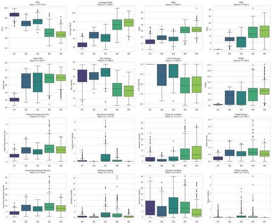
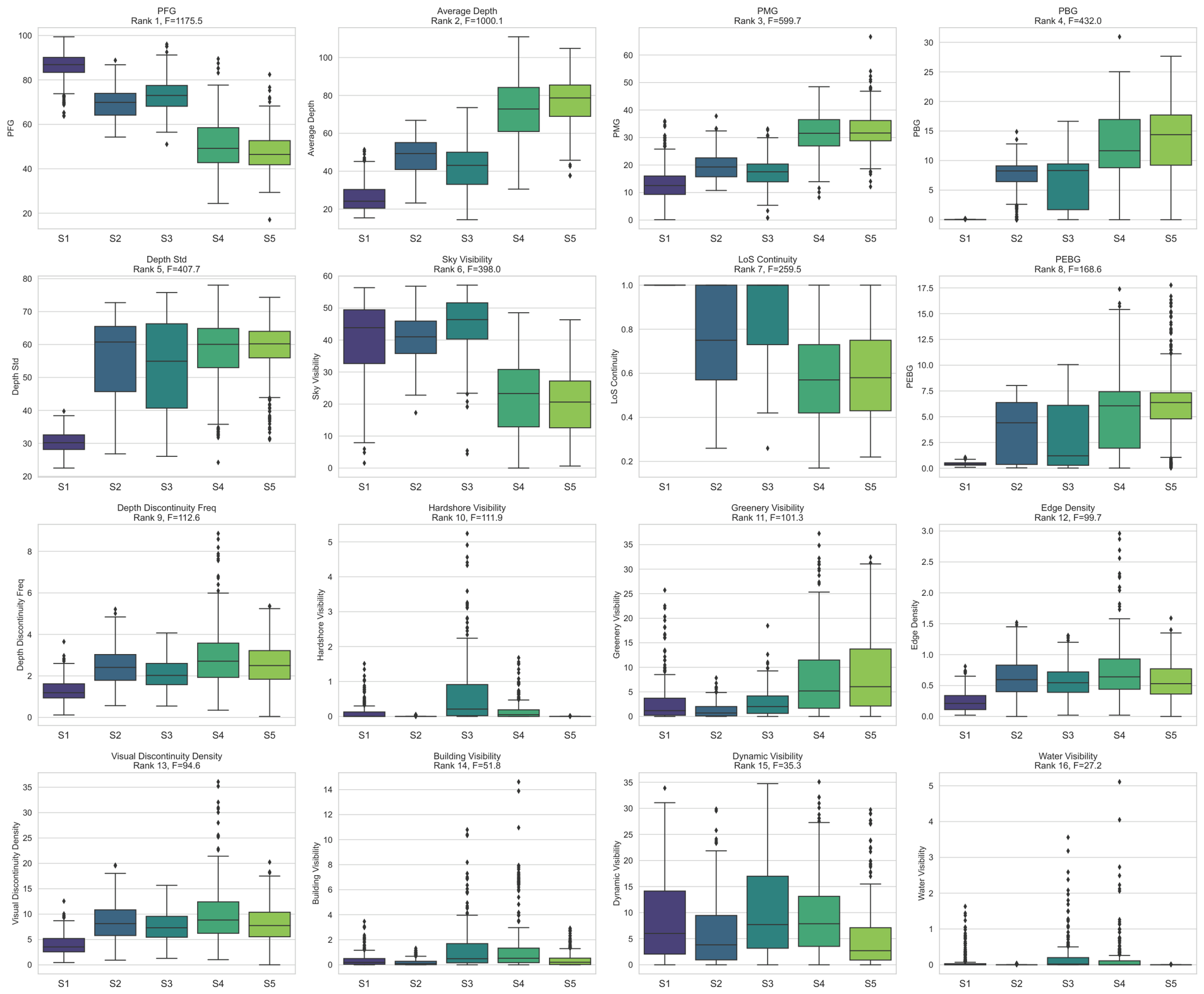
Clear differences were observed among the five latent states in the 16 visual–spatial features (Figure 5). One-way ANOVA showed that the biggest between-state differences were concentrated in depth-related and spatial-layering variables. Ranked by F-statistic, the top five features were PFG (F = 1295.0), Average Depth (F = 1108.9), PMG (F = 540.7), PBG (F = 522.9), and Depth Std (F = 468.5). This indicates that state differentiation was associated primarily with spatial layering, overall openness, and depth variation.

Among these features, PFG showed the strongest separation across states, with the highest median in S1 and the lowest in S5, highlighting its role in distinguishing foreground-dominant from more open environments. Average Depth also showed clear stratification, reaching its highest value in S2 and lowest value in S5, reflecting marked differences in perceived viewing distance and spatial openness across states.

4.2.3. Sequential Stability and Transition Dynamics of Latent States

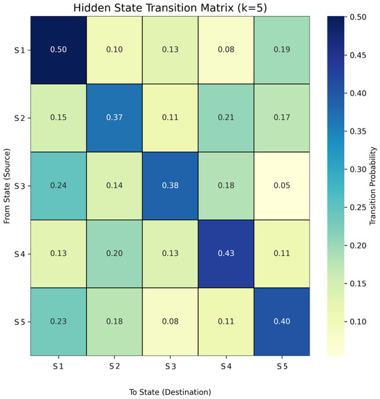
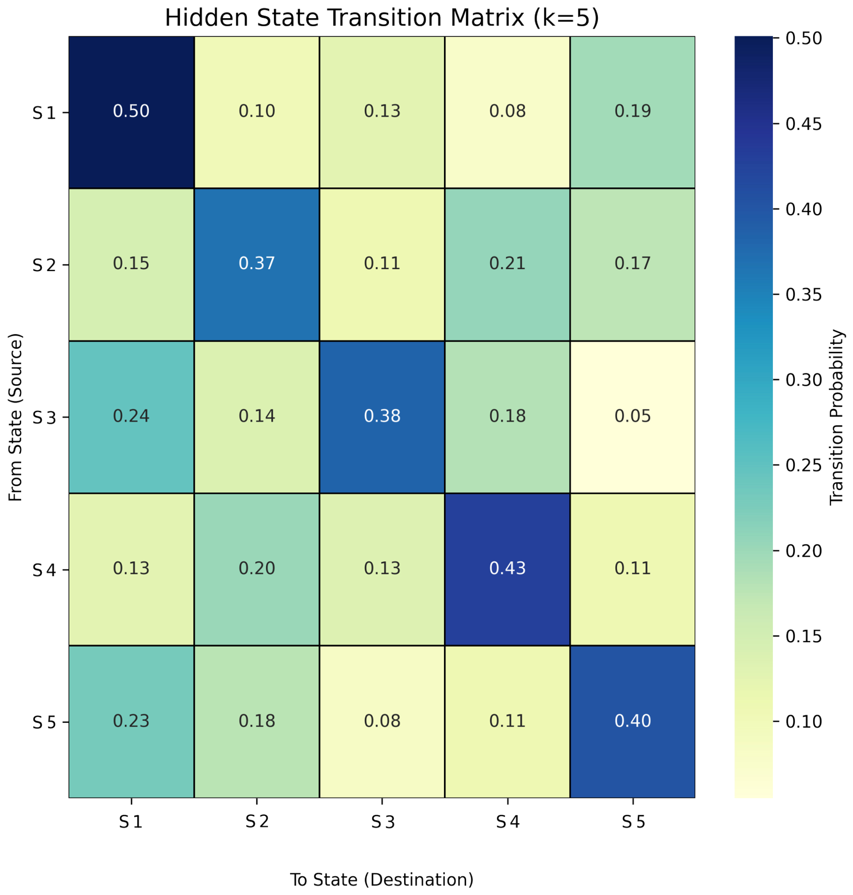
Self-transition probabilities were relatively high for all five latent states, indicating that they appeared as spatially continuous segments rather than as scattered observations along the corridor. The transition dynamics between different environments are further detailed in the probability matrix (Figure 6). S1 showed the highest self-transition probability (0.50), followed by S4 (0.43) and S5 (0.40), whereas S3 (0.38) and S2 (0.37) were slightly less stable. Overall, the state sequence exhibited clear continuity, suggesting that the corridor environment was organized into recognizable experiential sections.

Off-diagonal transitions were concentrated mainly between states with similar characteristics or transitional relationships, indicating gradual rather than abrupt environmental change along the corridor. The most prominent transitions included S2 to S5 (0.21), S3 to S1 (0.24), S3 to S4 (0.18), and S5 to S1 (0.23). These patterns show that open deep-view segments, vegetation-enhanced mixed spaces, and shallow enclosed environments were linked through recurrent transitions rather than existing as isolated types. More broadly, the transition matrix was concentrated near the diagonal, suggesting that state changes occurred primarily between adjacent or intermediate environments.

4.3. Semantic Interpretation of Latent States

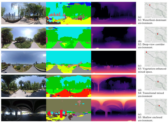
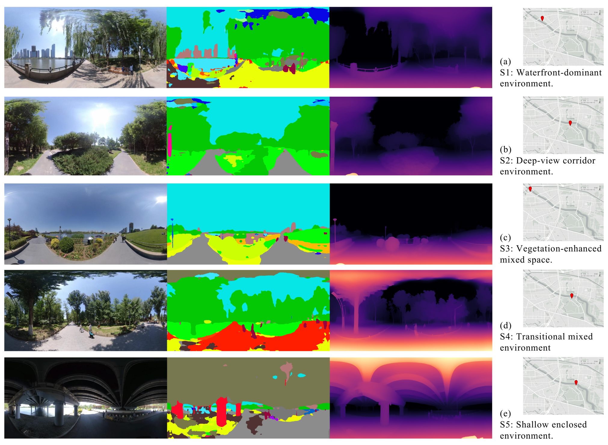
Based on the mean patterns of the 16 visual–spatial features across the five latent states, each state was semantically interpreted and named according to its dominant visual–spatial characteristics (Figure 7). These labels were defined primarily on the basis of environmental features, whereas behavioral differences are addressed in Section 4.4.

• S1: Waterfront-dominant environment.

S1 is characterized by a relatively high foreground proportion, together with moderate sky exposure and relatively abundant natural elements. It represents a near-field waterfront environment with clear spatial layering and a certain degree of enclosure.

• S2: Deep-view corridor environment.

S2 shows the highest Average Depth, relatively high Depth Std, and strong LoS Continuity. It represents an open and directional corridor environment with long perceived viewing distance.

• S3: Vegetation-enhanced mixed space.

S3 is marked by relatively high Greenery Visibility, moderately high PMG, and low Depth Discontinuity Freq. It represents a green mixed environment with relatively stable spatial interfaces and soft visual transitions.

• S4: Transitional mixed environment.

S4 remains close to the overall median on most core features, without being dominated by any single variable. It represents an intermediate mixed environment that links different spatial types along the corridor.

• S5: Shallow enclosed environment.

S5 is characterized by relatively low Average Depth and weak LoS Continuity, together with limited mid- to far-distance information. It represents a shallow and more enclosed environment with stronger near-range restriction.

Taken together, the five states were differentiated not only by semantic content but more importantly by depth-related spatial structure. S1 and S5 both contain stronger near-field conditions, but S1 is associated with clearer waterfront layering, whereas S5 is shallower and more visually constrained. S2 represents the opposite condition, with the greatest average depth and strongest directional continuity. S3 and S4 occupy intermediate positions, with S3 characterized by vegetation-enhanced midground stability and S4 functioning as a transitional mixed state. This differentiation shows that the HMM did not simply group images by visible objects, but identified interpretable visual–spatial configurations along the corridor sequence. In this sense, the five-state classification is one of the original outputs of the study, linking depth-informed spatial structure with sequential waterfront experience.

4.4. Visitor Behavior Across Latent States

4.4.1. Behavioral Differences Across Latent States

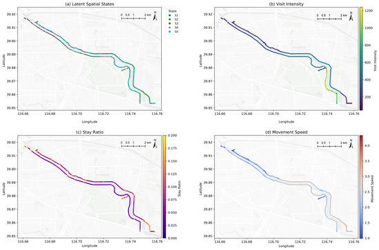
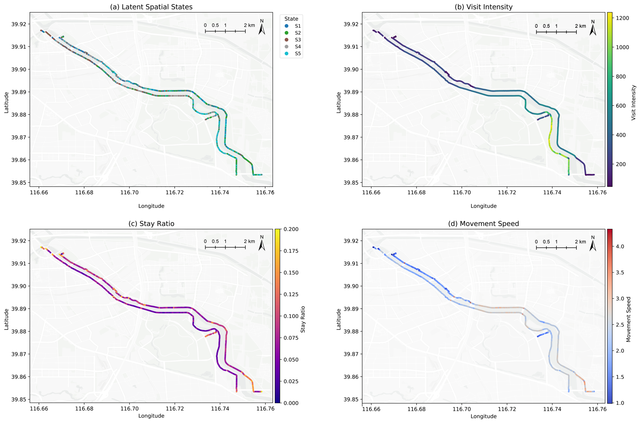
Visit intensity, stay ratio, and movement speed were used to describe three complementary behavioral dimensions: the spatial concentration of platform-recorded activity, the relative proportion of potential staying, and the pace of movement. Visitor behavior differed significantly across the five latent states. One-way ANOVA showed significant between-state differences in visit intensity (F = 45.67, p < 0.001), stay ratio (F = 9.93, p < 0.001), and movement speed (F = 28.36, p < 0.001). Visit intensity was highest in S5 (571.67), followed by S2 (475.94), whereas S1 (356.41) and S3 (333.78) were lower. Stay ratio was highest in S1 (0.069), followed by S2 (0.067) and S3 (0.063), whereas S4 (0.057) and S5 (0.053) were lower. Movement speed was highest in S2 (2.501), followed by S3 (2.439), whereas S1 (2.276), S4 (2.252), and S5 (2.250) were lower. These results show that the three behavioral dimensions formed differentiated patterns across states: S5 concentrated platform-recorded visits, S1 showed a stronger tendency toward potential staying, and S2 was associated with faster and more continuous movement.

4.4.2. Spatial Distribution of Visitor Behavior

Figure 8 integrates the spatial distribution of the five latent states with the three behavioral indicators. Taken together, the four panels show that visit intensity, stay ratio, and movement speed were spatially related but not coincident, forming a differentiated behavioral rhythm along the corridor. High visit intensity was concentrated mainly in the middle-to-late sections and around several turning nodes, where it overlapped considerably with S5 and part of S2. By contrast, a high stay ratio appeared more selectively in the initial section, at local turning points, and in some terminal segments, corresponding more closely to S1 and parts of S2 and S3. Higher movement speed occurred more often in continuous middle sections and downstream segments, where it was spatially closer to S2 and some S5 segments. Overall, the figure reinforces that visitor behavior along the corridor did not vary along a single intensity gradient, but differed across visiting, staying, and passing dimensions.

4.5. SHAP Analysis of State Differentiation

4.5.1. Overall Contribution Pattern of Visual–Spatial Indicators

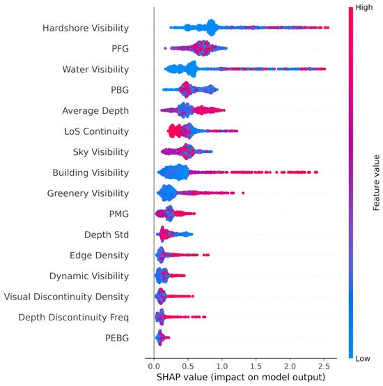
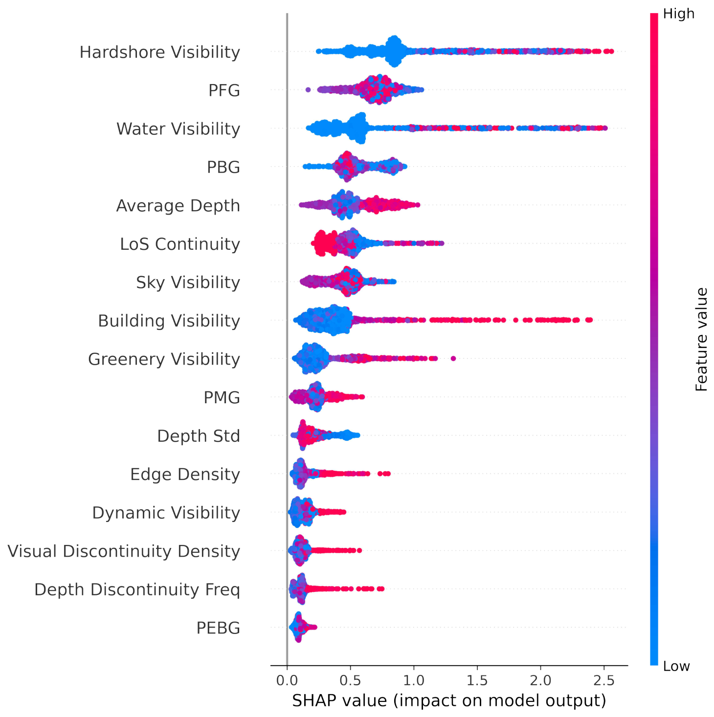
To evaluate the overall contribution of the 16 visual–spatial indicators to latent-state classification, SHAP analysis was introduced. As shown in Figure 9, feature importance exhibited a clearly uneven distribution. Hardshore Visibility, PFG, Water Visibility, and Average Depth ranked highest, whereas PEBG, Depth Discontinuity Freq, and Visual Discontinuity Density were located near the bottom of the ranking. This indicates that state classification relied more heavily on a limited number of key indicators rather than on the uniform contribution of all variables.

The highest-ranked indicators were mainly concentrated in two groups. One group consisted of variables related to spatial structure, especially foreground proportion and depth level. The other group comprised variables associated with waterfront interface conditions, mainly represented by hardshore visibility and water visibility. By contrast, variables describing local discontinuity or extreme background conditions contributed relatively little overall.

4.5.2. Differences in Feature Contributions Across States

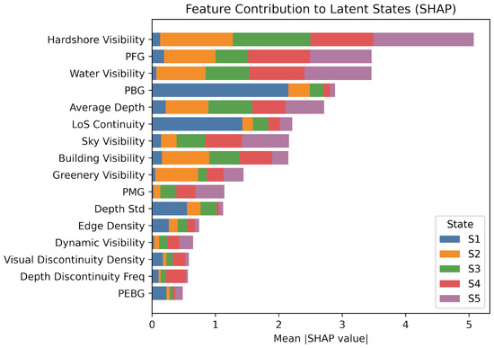
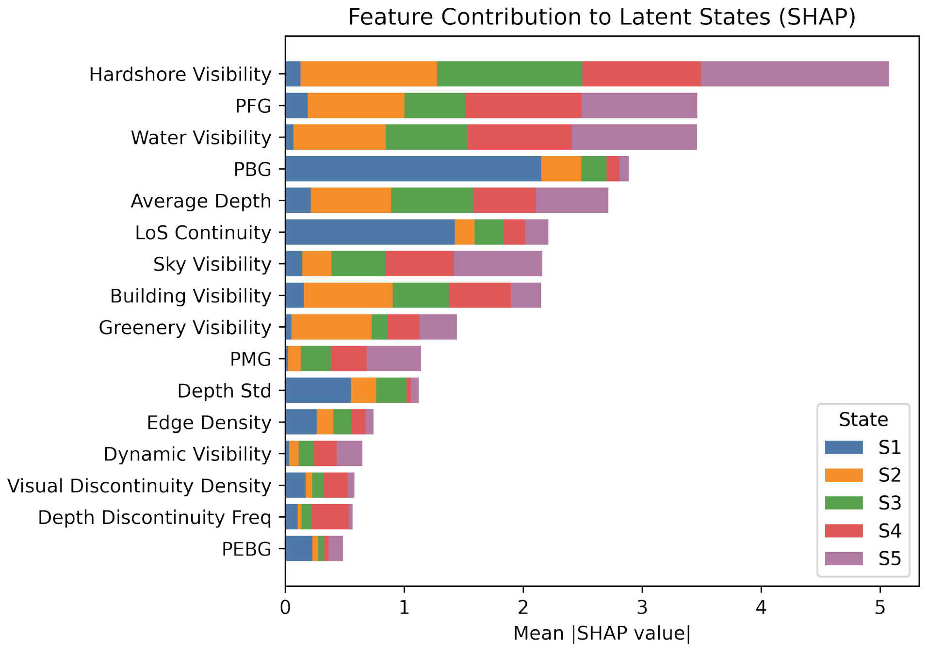
Although only a limited number of indicators dominated overall, the five latent states did not share the same contribution structure (Figure 10). Contributions for S1 and S3 were more concentrated, being characterized mainly by a small set of key indicators such as Hardshore Visibility, Water Visibility, PFG, and Average Depth. By contrast, contribution distributions for S2 and S4 were more dispersed, with no single absolutely dominant variable. S5 showed its largest SHAP contribution from Hardshore Visibility, indicating a waterfront-interface profile distinct from that of the other states.

These differences show that the five states were distinguished not by a single common feature, but by different combinations of key indicators. In other words, SHAP supports the interpretation that state differentiation emerged from structured variation in dominant visual–spatial features rather than from undifferentiated high-dimensional variation. At the same time, these results reflect model discrimination rather than direct causal effects.

5. Discussion

5.1. Mechanistic Interpretation of Visual–Spatial Structure

The results suggest that visual–spatial differentiation in the Grand Canal corridor is more closely associated with the structural organization of experienced space than with scene content alone. The HMM results show that the biggest between-state differences are concentrated in depth-related variables, especially foreground proportion, average depth, and depth layering. Because foreground proportion and average depth were highly collinear (r = −0.98), they should be interpreted as coupled indicators of near-field dominance and overall depth rather than as independent contributors. The SHAP analysis similarly identifies foreground/depth structure and waterfront-interface variables as important model-discriminating features for state differentiation. Together, these findings suggest that the corridor is differentiated not simply by what is visible, but by how space is organized and unfolds along the pedestrian path. This is consistent with recent arguments that image-based environmental assessment should move beyond object composition toward the structural organization of perceived space [48].

This pattern is especially important in linear waterfront corridors, where experience develops progressively through movement rather than from a single static viewpoint. In such settings, visitors not only perceive whether water, greenery, or built elements are present; they also encounter varying degrees of openness, enclosure, extension, and continuity [49]. In this study, a higher foreground proportion corresponded to stronger near-field presence and a shallower spatial condition, whereas greater average depth and stronger line-of-sight continuity corresponded to more open and directional environments. These variables therefore capture key perceptual dimensions of corridor experience: how close space feels, how far it extends, and how clearly it guides movement.

Waterfront-interface variables add a second layer to this mechanism. Although Water Visibility and Hardshore Visibility were low on average across the dataset, they showed strong discriminative value in state differentiation. Their importance therefore lies not in occupying a large share of the visual field overall but in marking meaningful shifts in spatial condition. In canal environments, whether water is visually accessible and whether the shoreline is expressed as a hard boundary can substantially alter perceived openness, edge definition, and the likelihood of lingering. The low mean values of these variables should also be understood in relation to the panoramic image format: because 360-degree images include the full surrounding visual field rather than a water-oriented view alone, waterfront elements may occupy a limited pixel proportion even when they are perceptually noticeable on site. The identified states thus reflect not only different depth structures, but also different combinations of spatial unfolding and waterfront-interface expression. This is broadly consistent with previous studies showing that waterfront perception depends not only on semantic imagery, but also on experiential qualities such as openness, naturalness, and environmental quality [29].

These findings help explain why two-dimensional semantic composition alone is insufficient for interpreting behavioral differences across corridor environments. Semantic indicators remain useful for describing environmental content, but they are less capable of explaining why some segments are associated with slowing, observation, or temporary staying, whereas others are associated with more direct and continuous movement. By contrast, variables related to foreground organization, depth structure, and interface continuity are more closely aligned with the spatial conditions through which behavior is organized. From this perspective, corridor environments are better understood as differences in spatial mechanism rather than differences in scene composition alone. In the Grand Canal corridor, experiential variation emerges from the joint action of depth layering, foreground structure, and waterfront interfaces, which together are related to how space is perceived sequentially during movement.

5.2. Sequential Spatial Logic of a Linear Green Waterfront Corridor

Unlike general urban open spaces, environmental experience in the Grand Canal corridor unfolds progressively and continuously along movement paths. Previous work on linear urban landscape has likewise emphasized that such environments should be understood through dynamic visual perception rather than through isolated static viewpoints, because what matters is not only what is seen at a given point, but how visual experience develops across a sequence of moving views [33,50].

The HMM results of this study show that all five latent states exhibit relatively high self-transition probabilities, and that transitions primarily occur between states with similar spatial characteristics or clear transitional relationships. This indicates that the visual–spatial environment of the Tongzhou section of the Grand Canal is characterized by strong continuity and gradual transformation along the corridor. In this sense, the spatial organization of the study area is better understood as a continuously evolving experiential process rather than as a simple aggregation of discrete landscape types.

From this perspective, the key issue is not only the differences among state types, but also how different spatial segments are connected and organized within a sequence [51]. States S1, S3, and S4 together represent a typical transition chain between natural interfaces and mixed environments, while S2 and S5 more clearly exhibit a rhythmic alternation between open, deep-view corridors and shallow, enclosed environments. In particular, the “deep–constricted” relationship between S2 and S5 suggests that spatial experience along the canal does not develop uniformly in a single direction, but instead evolves through repeated cycles of opening, constriction, and re-expansion. For visitors, such sequential variation may be associated with immediate visual perception, attention shifts, spatial anticipation, and route memory during movement.

Within this sequential logic, S4 plays a particularly critical role. It functions as a transitional segment within the experiential chain rather than merely representing an intermediate category in statistical terms. Its feature values are not extreme, its connections with other states are extensive, and its transition accessibility is relatively high. These characteristics indicate that S4 serves as a buffer, gateway, and reorganization segment between different spatial types. In the corridor, such segments often lack the strong identifiability of key nodes and the clear boundaries of highly open or enclosed environments, and are therefore easily overlooked in conventional spatial evaluations. However, from the perspective of continuous experience, these non-extreme segments are essential for maintaining the coherence of environmental transitions, enabling visitors to gradually perceive spatial change rather than encountering abrupt shifts between disconnected scenes.

This suggests that the spatial value of the corridor does not reside solely in prominent cultural nodes or highly recognizable scenes, but also in the continuous transitions, interface variations, and visual rhythms between them. For linear cultural landscapes such as the Grand Canal, what visitors actually experience is not a series of isolated places, but a continuous environmental process composed of interconnected state segments. Accordingly, the understanding of linear waterfront corridors can be extended from a “node-based cognition” toward a “sequence-based cognition,” in which spatial meaning emerges not only from individual locations but also from how these locations are connected, transitioned, and continuously experienced along movement paths.

5.3. Differentiation of Visitor Behavioral Rhythms

The behavioral results indicate that visitor responses to the corridor are organized through differentiated rhythms of visiting, staying, and passing. S5 showed the highest visit intensity, S1 the highest stay ratio, and S2 the highest movement speed. These patterns suggest that different visual–spatial states are associated with different forms of use within the corridor and that visitor behavior unfolds through multiple behavioral dimensions. This interpretation is consistent with recent studies showing that recreational use in river corridors and park environments is expressed through differentiated activity types and is associated with distinct spatial and environmental conditions [42,52]. Building on this line of evidence, our results further show that such behavioral differentiation can be understood within a sequential visual–spatial framework, in which different corridor segments correspond to different behavioral patterns of movement, slowing, and temporary staying.

Firstly, the spatial conditions associated with movement concentration differed from those associated with temporary staying. The high visit intensity observed in S5 suggests that this type of environment was associated with the concentration and passage of movement flows. By contrast, S1 showed the highest stay ratio despite not attracting the highest visitor volume. This pattern indicates that environments with stronger foreground presence, clearer near-field layering, and perceptible waterfront interfaces were associated with pausing, short-term observation, and temporary staying. In this sense, movement concentration and temporary staying were linked to different corridor conditions.

Secondly, the pattern of S2 suggests that relatively high movement speed can coexist with a meaningful corridor experience. S2 combined the highest speed with relatively high visit intensity, indicating that open and directional corridor environments were associated with efficient passage while remaining spatially legible and experientially relevant. Greater depth and stronger line-of-sight continuity likely enhanced forward extension and directional clarity, and may correspond to a smoother movement rhythm. In corridor settings, such segments are therefore better understood as guidance-oriented spaces that are associated with continuous movement.

Thirdly, lower movement speed reflected multiple behavioral processes across states. In S1, slower movement was accompanied by a higher stay ratio, indicating deceleration related to observation and temporary stopping. In S3, lower speed was more consistent with a steady and relatively leisurely walking rhythm in a softer and more stable spatial setting. In S4, lower speed appeared mainly in transitional segments, suggesting adjustment during spatial change. These differences show that lower speed may correspond to temporary staying, exploratory walking, or transition-related adjustment, depending on the spatial context.

From this perspective, visitor behavior in the corridor is better understood as a rhythmically differentiated structure organized by visual–spatial states. Different segments may correspond to concentration, guidance, buffering, observation, or temporary staying, and together form a continuous experiential process along the corridor. This also suggests that corridor optimization should pay attention not only to prominent nodes, but also to how different segments are associated with different behavioral functions within the sequence of movement.

5.4. Planning and Design Implications

These findings also provide practical implications for the planning and management of linear green waterfront corridors. Rather than treating the corridor as a collection of isolated scenic nodes, the results suggest that it should be understood as a continuous sequence of differentiated visual–spatial conditions. The five latent states identified in this study indicate that different corridor segments are associated with different spatial and behavioral patterns. Waterfront-dominant environments may provide opportunities for short-term observation and waterside staying; deep-view corridor environments may be suitable for route legibility and continuous movement; vegetation-enhanced mixed spaces may contribute to recreational comfort; transitional mixed environments may help maintain continuity between contrasting spatial conditions; and shallow enclosed environments with high trajectory-recorded visit intensity may require greater attention to visibility, safety, and crowd dispersion.

From this perspective, planning strategies for waterfront corridors should not focus only on prominent nodes or high-use areas, but should also consider how different spatial states are arranged and connected along the route. Design and management interventions should therefore be adapted to the role of each segment within the sequence: strengthening water visibility and edge comfort where staying is likely, preserving openness and sightline continuity where movement guidance is important, balancing vegetation enclosure with safety and visibility in recreational segments, and improving circulation clarity in constrained high-intensity segments. In this way, the latent visual–spatial state framework can support a more sequence-based approach to waterfront corridor planning, linking visual–spatial structure with observed patterns of movement and staying.

6. Conclusions

In the present study, we make three main contributions. First, we identify the Grand Canal corridor as a sequence of latent visual–spatial states distributed along movement paths, with clear continuity and gradual transitions. Second, we show that visitor behavior varies systematically across these states, with different corridor segments associated with different behavioral patterns, including movement concentration, guided passage, transitional adjustment, and temporary staying. Third, we demonstrate that depth-informed structural variables, especially the closely related foreground proportion and average depth, together with waterfront-interface conditions, are the strongest model-discriminating features for state differentiation. Methodologically, we develop an integrated framework combining monocular depth estimation, semantic segmentation, Hidden Markov modeling, trajectory-based behavioral analysis, and SHAP interpretation. Several limitations remain, including possible user bias in platform-based trajectory data, the use of a single case area, and the absence of explicit temporal modeling. Future research should test this framework across multiple waterfront and non-waterfront green corridors, incorporate more diverse behavioral and temporal data, and further examine how proximity to water is associated with movement, potential staying, and the transferability of latent visual–spatial state analysis across urban open-space contexts.

References

- Liu, Z.; Lin, Y.; De Meulder, B.; Wang, S. Can Greenways Perform as a New Planning Strategy in the Pearl River Delta, China? Landsc. Urban Plan. 2019, 187, 81–95. [Google Scholar] [CrossRef] [Scilit]
- Ahern, J. Green Infrastructure for Cities: The Spatial Dimension. In Cities of the Future: Towards Integrated Sustainable Water and Landscape Management; IWA Publishing: London, UK, 2007; pp. 267–283. [Google Scholar]
- Liu, X.; Chen, X.; Huang, Y.; Wang, W.; Zhang, M.; Jin, Y. Landscape Aesthetic Value of Waterfront Green Space Based on Space–Psychology–Behavior Dimension: A Case Study along Qiantang River (Hangzhou Section). Int. J. Environ. Res. Public Health 2023, 20, 3115. [Google Scholar] [CrossRef] [Scilit] [PubMed]
- Hartig, T.; Mitchell, R.; De Vries, S.; Frumkin, H. Nature and Health. Annu. Rev. Public Health 2014, 35, 207–228. [Google Scholar] [CrossRef] [Scilit] [PubMed]
- Kabisch, N.; Qureshi, S.; Haase, D. Human–Environment Interactions in Urban Green Spaces—A Systematic Review of Contemporary Issues and Prospects for Future Research. Environ. Impact Assess. Rev. 2015, 50, 25–34. [Google Scholar] [CrossRef] [Scilit]
- Liu, S.; Lai, S.-Q.; Liu, C.; Jiang, L. What Influenced the Vitality of the Waterfront Open Space? A Case Study of Huangpu River in Shanghai, China. Cities 2021, 114, 103197. [Google Scholar] [CrossRef] [Scilit]
- Gobster, P.H.; Westphal, L.M. The Human Dimensions of Urban Greenways: Planning for Recreation and Related Experiences. Landsc. Urban Plan. 2004, 68, 147–165. [Google Scholar] [CrossRef] [Scilit]
- Durán Vian, F.; Pons Izquierdo, J.J.; Serrano Martínez, M. River-City Recreational Interaction: A Classification of Urban Riverfront Parks and Walks. Urban For. Urban Green. 2021, 59, 127042. [Google Scholar] [CrossRef] [Scilit]
- Flemsæter, F.; Stokowski, P.; Frisvoll, S. The Rhythms of Canal Tourism: Synchronizing the Host-Visitor Interface. J. Rural Stud. 2020, 78, 199–210. [Google Scholar] [CrossRef] [Scilit]
- Mears, M.; Brindley, P.; Barrows, P.; Richardson, M.; Maheswaran, R. Mapping Urban Greenspace Use from Mobile Phone GPS Data. PLoS ONE 2021, 16, e0248622. [Google Scholar] [CrossRef] [Scilit]
- Zhou, H.; Wang, J.; Wilson, K. Impacts of Perceived Safety and Beauty of Park Environments on Time Spent in Parks: Examining the Potential of Street View Imagery and Phone-Based GPS Data. Int. J. Appl. Earth Obs. Geoinf. 2022, 115, 103078. [Google Scholar] [CrossRef] [Scilit]
- Encalada-Abarca, L.; Ferreira, C.C.; Rocha, J. Revisiting City Tourism in the Longer Run: An Exploratory Analysis Based on LBSN Data. Curr. Issues Tour. 2024, 27, 584–599. [Google Scholar] [CrossRef] [Scilit]
- Liu, W.; Wang, B.; Yang, Y.; Mou, N.; Zheng, Y.; Zhang, L.; Yang, T. Cluster Analysis of Microscopic Spatio-Temporal Patterns of Tourists’ Movement Behaviors in Mountainous Scenic Areas Using Open GPS-Trajectory Data. Tour. Manag. 2022, 93, 104614. [Google Scholar] [CrossRef] [Scilit]
- Luo, P.; Yu, B.; Li, P.; Liang, P. Spatially Varying Impacts of the Built Environment on Physical Activity from a Human-Scale View: Using Street View Data. Front. Environ. Sci. 2022, 10, 1021081. [Google Scholar] [CrossRef] [Scilit]
- Yang, X.; Zhang, C.; Yang, L. Revealing Spatial Patterns and Environmental Influences on Jogging Volume and Speed: Insights from Crowd-Sourced GPS Trajectory Data and Random Forest. ISPRS Int. J. Geo-Inf. 2025, 14, 80. [Google Scholar] [CrossRef] [Scilit]
- Appleton, J. The Experience of Landscape; John Wiley & Sons: Chichester, UK, 1975; ISBN 0-471-03256-5. [Google Scholar]
- Appleton, J. Prospects and Refuges Re-Visited. Landsc. J. 1984, 3, 91–103. [Google Scholar] [CrossRef] [Scilit]
- Biederman, I. Recognition-by-Components: A Theory of Human Image Understanding. Psychol. Rev. 1987, 94, 115–147. [Google Scholar] [CrossRef] [Scilit]
- Kaplan, R.; Kaplan, S. The Experience of Nature: A Psychological Perspective; Cambridge University Press: Cambridge, MA, USA; New York, NY, USA, 1989. [Google Scholar]
- Biljecki, F.; Ito, K. Street View Imagery in Urban Analytics and GIS: A Review. Landsc. Urban Plan. 2021, 215, 104217. [Google Scholar] [CrossRef] [Scilit]
- Turner, A.; Doxa, M.; O’Sullivan, D.; Penn, A. From Isovists to Visibility Graphs: A Methodology for the Analysis of Architectural Space. Environ. Plan. B Plan. Des. 2001, 28, 103–121. [Google Scholar] [CrossRef] [Scilit]
- Xia, Y.; Yabuki, N.; Fukuda, T. Development of a System for Assessing the Quality of Urban Street-Level Greenery Using Street View Images and Deep Learning. Urban For. Urban Green. 2021, 59, 126995. [Google Scholar] [CrossRef] [Scilit]
- Seresinhe, C.I.; Preis, T.; MacKerron, G.; Moat, H.S. Happiness Is Greater in More Scenic Locations. Sci. Rep. 2019, 9, 4498. [Google Scholar] [CrossRef] [Scilit]
- Lu, Y. Using Google Street View to Investigate the Association between Street Greenery and Physical Activity. Landsc. Urban Plan. 2019, 191, 103435. [Google Scholar] [CrossRef] [Scilit]
- Zhang, F.; Zhou, B.; Liu, L.; Liu, Y.; Fung, H.H.; Lin, H.; Ratti, C. Measuring Human Perceptions of a Large-Scale Urban Region Using Machine Learning. Landsc. Urban Plan. 2018, 180, 148–160. [Google Scholar] [CrossRef] [Scilit]
- Fan, Z.; Zhang, F.; Loo, B.P.Y.; Ratti, C. Urban Visual Intelligence: Uncovering Hidden City Profiles with Street View Images. Proc. Natl. Acad. Sci. USA 2023, 120, e2220417120. [Google Scholar] [CrossRef] [Scilit] [PubMed]
- Yang, N.; Deng, Z.; Hu, F.; Guan, Q.; Chao, Y.; Wan, L. Urban Perception Assessment from Street View Images Based on a Multifeature Integration Encompassing Human Visual Attention. Ann. Am. Assoc. Geogr. 2024, 114, 1424–1442. [Google Scholar] [CrossRef] [Scilit]
- Cao, Y.; Yang, P.; Xu, M.; Li, M.; Li, Y.; Guo, R. A Novel Method of Urban Landscape Perception Based on Biological Vision Process. Landsc. Urban Plan. 2025, 254, 105246. [Google Scholar] [CrossRef] [Scilit]
- Luo, J.; Zhao, T.; Cao, L.; Biljecki, F. Water View Imagery: Perception and Evaluation of Urban Waterscapes Worldwide. Ecol. Indic. 2022, 145, 109615. [Google Scholar] [CrossRef] [Scilit]
- Biscaya, S.; Elkadi, H. A Smart Ecological Urban Corridor for the Manchester Ship Canal. Cities 2021, 110, 103042. [Google Scholar] [CrossRef] [Scilit]
- Dong, W.; Kang, Q.; Wang, G.; Hou, R.; Liu, P. Exploring the Influence of Path Environment Factors on Walking Behavior in Urban Parks with Configuration Attribute Control. PLoS ONE 2025, 20, e0329278. [Google Scholar] [CrossRef] [Scilit]
- Zhou, X.; Cen, Q.; Qiu, H. Effects of Urban Waterfront Park Landscape Elements on Visual Behavior and Public Preference: Evidence from Eye-Tracking Experiments. Urban For. Urban Green. 2023, 82, 127889. [Google Scholar] [CrossRef] [Scilit]
- Chen, J.; Zhao, X.; Wang, H.; Yan, J.; Yang, D.; Xie, K. Portraying Heritage Corridor Dynamics and Cultivating Conservation Strategies Based on Environment Spatial Model: An Integration of Multi-Source Data and Image Semantic Segmentation. Herit. Sci. 2024, 12, 419. [Google Scholar] [CrossRef] [Scilit]
- Li, Y.; Cao, L.; Gao, W. Perceptual Dimensions of Heritage Canal Landscapes and Their Impact on Conservation Value Cognition. Ecol. Indic. 2025, 176, 113626. [Google Scholar] [CrossRef] [Scilit]
- Sun, Y.; Xi, X.; Lyu, N. Research on the Route Selection Method of the Grand Canal National Trails for Central Urban Areas: A Case Study of the Grand Canal, the Old Town of Jining City Section, China. Land 2025, 14, 1053. [Google Scholar] [CrossRef] [Scilit]
- Nagata, S.; Nakaya, T.; Hanibuchi, T.; Amagasa, S.; Kikuchi, H.; Inoue, S. Objective Scoring of Streetscape Walkability Related to Leisure Walking: Statistical Modeling Approach with Semantic Segmentation of Google Street View Images. Health Place 2020, 66, 102428. [Google Scholar] [CrossRef] [Scilit]
- Ranftl, R.; Bochkovskiy, A.; Koltun, V. Vision Transformers for Dense Prediction. In Proceedings of the 2021 IEEE/CVF International Conference on Computer Vision (ICCV), Montreal, QC, Canada, 11–17 October 2021; pp. 12159–12168. [Google Scholar]
- Yang, L.; Kang, B.; Huang, Z.; Zhao, Z.; Xu, X.; Feng, J.; Zhao, H. Depth Anything V2. In Advances in Neural Information Processing Systems 37 (NeurIPS 2024); NeurIPS: Vancouver, BC, Canada, 2024. [Google Scholar]
- Jeong, S.; Kang, Y.; Lee, J.; Sohn, K. Variational Embedding of a Hidden Markov Model to Generate Human Activity Sequences. Transp. Res. Part C Emerg. Technol. 2021, 131, 103347. [Google Scholar] [CrossRef] [Scilit]
- Shin, D.-W.; Yang, C.-S. Classification of Ship Type from Combination of HMM–DNN–CNN Models Based on Ship Trajectory Features. Remote Sens. 2024, 16, 4245. [Google Scholar] [CrossRef] [Scilit]
- Zeng, Z.; Qin, J.; Wu, T. A Knowledge Graph-Enhanced Hidden Markov Model for Personalized Travel Routing: Integrating Spatial and Semantic Data in Urban Environments. Smart Cities 2025, 8, 75. [Google Scholar] [CrossRef] [Scilit]
- Shi, H.; Zhang, L.; Ma, D.; Zhang, M.; Wang, M.; Wei, Z. Exploring Recreational Walking and Its Correlated Built Environment Factors in River Corridor Space through a Trajectory Sematic-Based Approach. Urban For. Urban Green. 2025, 107, 128767. [Google Scholar] [CrossRef] [Scilit]
- Mao, L.; Hou, H.; Xia, Z.; Zhang, X. Soundscape Preferences and Cultural Ecosystem Services in the Grand Canal National Cultural Park: A Case Study of Tongzhou Forest Park. Buildings 2025, 15, 2360. [Google Scholar] [CrossRef] [Scilit]
- Cui, J.; Zhang, S.; Wang, L. Evaluating Canal Heritage Tourists’ Satisfaction: An Asymmetric Impact-Performance Analysis of the Grand Canal in Beijing, China. J. Hosp. Tour. Manag. 2025, 62, 108–115. [Google Scholar] [CrossRef] [Scilit]
- Zhao, M.; Zhang, Q.; Shi, H.; Liu, M.; Liang, J. Exploring the Spatial Characteristics of Stay Areas in Walking Tours through the Lens of Volunteered GPS Trajectories: A Case Study of the Zhuhai–Macao Metropolitan Area. Forests 2022, 13, 1800. [Google Scholar] [CrossRef] [Scilit]
- Zhou, B.; Zhao, H.; Puig, X.; Fidler, S.; Barriuso, A.; Torralba, A. Scene Parsing through ADE20K Dataset. In Proceedings of the 2017 IEEE Conference on Computer Vision and Pattern Recognition (CVPR), Honolulu, HI, USA, 21–26 July 2017; pp. 5122–5130. [Google Scholar]
- Lundberg, S.M.; Lee, S.-I. A Unified Approach to Interpreting Model Predictions; Curran Associates, Inc.: New York, NY, USA, 2017; Volume 30, pp. 4765–4774. [Google Scholar]
- Zhang, X.; Lin, E.S.; Tan, P.Y.; Qi, J.; Waykool, R. Assessment of Visual Landscape Quality of Urban Green Spaces Using Image-Based Metrics Derived from Perceived Sensory Dimensions. Environ. Impact Assess. Rev. 2023, 102, 107200. [Google Scholar] [CrossRef] [Scilit]
- Stoltz, J.; Grahn, P. Perceived Sensory Dimensions: An Evidence-Based Approach to Greenspace Aesthetics. Urban For. Urban Green. 2021, 59, 126989. [Google Scholar] [CrossRef] [Scilit]
- Jin, X.; Wang, J. Assessing Linear Urban Landscape from Dynamic Visual Perception Based on Urban Morphology. Front. Archit. Res. 2021, 10, 202–219. [Google Scholar] [CrossRef] [Scilit]
- Liu, M.; Nijhuis, S. Mapping Landscape Spaces: Methods for Understanding Spatial-Visual Characteristics in Landscape Design. Environ. Impact Assess. Rev. 2020, 82, 106376. [Google Scholar] [CrossRef] [Scilit]
- Zhang, W.; Guan, H.; Li, S.; Huang, B.; Hong, W.; Liu, W. The Impact of Street-Scale Built Environments on Urban Park Visitations: A Case Study in Wuhan. Appl. Geogr. 2024, 171, 103374. [Google Scholar] [CrossRef] [Scilit]
Disclaimer/Publisher’s Note: The statements, opinions and data contained in all publications are solely those of the individual author(s) and contributor(s) and not of MDPI and/or the editor(s). MDPI and/or the editor(s) disclaim responsibility for any injury to people or property resulting from any ideas, methods, instructions or products referred to in the content. |
© 2026 by the authors. Licensee MDPI, Basel, Switzerland. This article is an open access article distributed under the terms and conditions of the Creative Commons Attribution (CC BY) license.