


Abstract
This study introduces a domain-specific multimodal deep learning framework, centered on a Vision Transformer (ViT), to accelerate the prediction of operational carbon emissions in residential buildings. Our approach uniquely fuses two data modalities: the geometric information captured in floorplan images and the quantitative data from vector-based building parameters. By training and testing on a comprehensive dataset of 17,000 residential samples derived from a large-scale open-source Chinese database, the proposed model demonstrates exceptional predictive capability. On the test set, it achieved a mean bias error of 1.75%, a mean absolute percentage error of 2.14%, and a coefficient of determination (R2) of 0.95. Further validation through comparative analysis shows that our framework significantly outperforms established deep learning architectures, including ResNet-18, Inception-V4, and VGG-19, in both accuracy and robustness. The developed tool provides architects with a reliable and rapid method for assessing the carbon footprint of design options, thereby offering crucial scientific support for sustainable building design.
1. Introduction
1.1. Background
Addressing global climate and energy challenges necessitates a focus on energy conservation and decarbonization. In China, the building industry is a major contributor, responsible for over 46.5% of national energy use and about 6.0% of global consumption, making it a pivotal sector for achieving the country’s 2030 carbon peak and 2060 carbon neutrality targets [1]. Within a building’s life cycle, the operational phase is particularly significant, contributing to roughly 25% of China’s total energy demand and representing a primary opportunity for emission mitigation [2,3,4]. This issue is compounded by rapid urbanization and the expansion of residential housing, which drive further increases in energy use and carbon output [5,6]. The hot-summer and cold-winter climate zone, exemplified by the Yangtze River Delta, presents a unique case with its high-density housing, older building stock, and substantial, yet largely untapped, potential for carbon reduction [7,8].
The analysis of building carbon emissions relies heavily on performance assessment and prediction. Traditionally, two primary methods have been employed for forecasting operational carbon emissions (OCEs): physics-based simulation and statistical regression modeling [9,10,11]. Simulation tools, while established, require intricate model setup and extensive computation time, making them impractical for rapid feedback during the early design stages [12,13,14,15]. In contrast, machine learning offers a powerful alternative by establishing direct, non-linear mappings between design inputs and performance outcomes [16,17,18,19,20]. These data-driven models can dramatically shorten evaluation cycles and reduce costs without sacrificing predictive power. Different machine learning techniques are suited for different data types; for instance, regression algorithms are effective for structured vector data, while deep learning excels at interpreting unstructured image data [21,22,23]. By leveraging these advanced computational methods, architects and stakeholders can receive timely and actionable insights to guide design decisions.
The built environment is inherently multimodal, characterized by a rich combination of geometric and non-geometric information. Its spatial form, from the macro-level urban context to the micro-level interior layout, can be represented through diverse data formats like vectors, images, and graphs [24,25,26]. For example, while vector data can precisely define material properties or climate variables, image data is superior at capturing the holistic geometric and spatial qualities of a design. The limitations of existing methods can compromise a model’s ability to generalize and accurately capture the complex interplay of factors influencing building performance [27,28,29]. Consequently, developing predictive frameworks that can integrate and leverage multimodal information is essential for improving their accuracy and applicability.
1.2. Related Work
1.2.1. Evolution of Data-Driven Carbon Prediction Models
The application of machine learning to building performance prediction has evolved through distinct phases, primarily defined by the type of data utilized. The initial wave of research focused on traditional regression models and shallow neural networks, which operate on structured, vector-based data. Algorithms such as multiple linear regression, support vector regression (SVR), Random Forest, and Multilayer Perceptions (MLPs) have been widely employed to forecast building energy consumption and carbon emissions [30,31,32,33]. These models excel at identifying correlations within tabular datasets. For instance, Huang et al. [34] conducted a comparative study across 34 Chinese cities and concluded that gradient boosting models demonstrated superior performance for predicting operational carbon emissions (OCEs) from structured building parameters. Similarly, Zheng et al. [35] developed a highly accurate prediction model for residential buildings in Guangzhou by incorporating vector data related to actual resident behavior. However, a limitation of these vector-centric models is their reliance on pre-defined, abstract parameters to represent a building. This process of ‘feature engineering’ inevitably results in information loss, as the complex spatial and topological nuances of a building’s layout are distilled into simplified metrics (e.g., shape factor, window-to-wall ratio).
To address this, a subsequent wave of research turned to deep learning, particularly Convolutional Neural Networks (CNNs), which can directly process image-based representations like floorplans. By automatically extracting hierarchical spatial features, CNN-based models can understand the geometry that vector-only models cannot [36,37]. Yet, a purely image-based approach creates its own informational silo. While CNNs excel at interpreting geometry, they remain blind to crucial non-visual parameters that heavily influence energy performance, such as wall insulation properties, window U-values, or specific climatic conditions [38,39]. This inherent dichotomy exposes a clear research gap and underscores the necessity for a model that can synergistically process both data modalities [33,40,41,42,43].
Quantitative evidence from recent studies highlights this limitation. For instance, models relying solely on structured building parameters (vector-only) typically achieve an R2 between 0.82 and 0.89, struggling to account for over 10% of the variance attributed to complex spatial geometry. Conversely, pure image-based models often reach a performance plateau because they neglect non-visual thermal properties, such as insulation U-values, which can influence OCEs by up to 25%. This performance gap underscores that neither modality alone can encapsulate the full complexity of building carbon performance.
1.2.2. Bridging the Modality Gap with Multimodal Learning
To overcome the limitations of unimodal systems, researchers have increasingly explored multimodal machine learning, which seeks to create a more holistic building representation by integrating disparate data sources. The core principle is that fusing different data types allows a model to form a more comprehensive understanding, leading to enhanced accuracy and generalization over single-modal counterparts.
These pioneering studies validate the potential of multimodal fusion in the built environment. For example, Li et al. [44] developed a generative adversarial network that fused floorplan and facade images to predict daylighting, demonstrating how different visual inputs could be combined. In another study, Fujiwara et al. [45] successfully predicted microclimate data by fusing street-level imagery with meteorological sensor data, showcasing a vector-and-image fusion approach. Meanwhile, Jiang et al. [46] employed a similar fusion strategy for the generative task of urban layout synthesis. While these efforts are promising, their application to the predictive task of building carbon emissions remains limited. Furthermore, many of these frameworks rely on CNNs for image processing, which, due to their localized receptive fields, may not be optimal for capturing the global context of an entire building layout.
Predicting operational carbon requires a global understanding of the floorplan—how the arrangement of rooms on one side of the building affects the other, or how the overall form interacts with solar paths. This is where the Vision Transformer (ViT) architecture offers a distinct advantage. Standard CNN-based frameworks are inherently limited by their local inductive bias, processing images through a restricted window that fails to recognize global topological relationships. In architectural science, this is a critical flaw: the energy balance of a floorplan is a globally coupled system where, for example, the solar gain from a southern facade directly dictates the heating demand of northern thermal zones [47,48]. ViT addresses this by replacing local convolutions with a global self-attention mechanism, allowing the model to simultaneously weigh dependencies across the entire planform. This shifts the modeling paradigm from local texture recognition to holistic spatial reasoning.
Moreover, the token-based nature of ViT provides a conceptually elegant framework for multimodal fusion. Both image patches (from the floorplan) and vector-based parameters (building physics and climate) can be projected into a shared embedding space and treated as a unified sequence of tokens [49,50]. This allows the model to learn complex cross-modal interactions through its self-attention layers, effectively enabling different data types to “attend” to one another. Therefore, we hypothesize that a ViT-based multimodal framework is uniquely suited to creating a comprehensive, robust, and accurate model for operational carbon prediction.
1.3. Objectives and Innovations
This study aims to overcome the practical challenges in the early-stage design using unimodal approaches by developing a framework that synergistically processes a building’s geometric form and its physical parameters. Our work is defined by two primary objectives, which also represent its core innovations:
- (1)
- Developing a multimodal data processing method for residential buildings: This study proposes a systematic method that fuses large-scale architectural layouts from the ResPlan dataset with engineering parameters compliant with China’s design codes, constructing a high-quality benchmark dataset of 17,000 samples. This provides a reliable data foundation for data-driven building performance analysis.
- (2)
- Proposing and validating a ViT-based deep fusion prediction architecture: The core technical innovation of this study lies in leveraging the self-attention mechanism of ViT to capture global spatial dependencies within floorplans, overcoming the local bias limitations of traditional CNNs. The framework adopts a unified approach that projects both image patches and vector parameters into a shared embedding space to enable deep cross-modal interactions. Comparative experiments against mainstream CNN baselines validate the superiority of this architecture in prediction accuracy and robustness.
2. Method
The methodology of this study is structured around a systematic, multi-stage workflow designed to develop and rigorously validate the proposed multimodal ViT prediction framework, as illustrated in Figure 1. The workflow begins with the foundational step of constructing a large-scale benchmark dataset. This involves programmatically generating 17,000 unique residential building designs by pairing floorplans from the ResPlan dataset with a wide range of physical and climatic parameters. Subsequently, high-fidelity operational carbon emission labels for each design are generated using validated physics-based simulations (EnergyPlus), establishing the ground-truth data for model training.
Figure 1.
Research framework.
With the dataset established, the core of the methodology focuses on the development, training, and evaluation of the multimodal ViT model. This encompasses the design of the model’s architecture, hyperparameter optimization, and a rigorous validation phase. To contextualize its performance, the proposed model is benchmarked against several established deep learning architectures, allowing for a comprehensive comparative analysis of its predictive accuracy and robustness. This integrated approach ensures that the final framework is not only accurate but also validated against current state-of-the-art methods, making it a reliable tool for early-stage design assessment.
2.1. Generation of a Multimodal Benchmark Dataset
The predictive power of the proposed framework is contingent upon a high-quality, large-scale multimodal dataset. This dataset was methodically constructed by synthesizing three distinct data streams: (1) geometric information from architectural layouts, (2) physical properties defined by building parameters, and (3) environmental context from climatic data. This synthesis process ensures that each of the 17,000 samples represents a unique and plausible building instance, where a specific floorplan image is paired with a corresponding vector of engineering and climatic variables. The generation of this dataset was guided by principles of diversity and realism, achieved through probabilistic sampling of parameters within ranges compliant with regional design codes. This approach guarantees that the resulting dataset is not only comprehensive but also representative of the design possibilities within the specified climate zone, thereby providing a robust foundation for training a generalizable prediction model.
The selection of a massive dataset is a deliberate strategic choice to enhance the model’s robustness. By training on 17,000 unique samples, the framework is exposed to a vast spectrum of architectural configurations, which significantly mitigates the risk of overfitting to specific geometric patterns. This large-scale diversity ensures that the model learns the underlying physics-spatial correlations rather than memorizing a limited set of synthetic samples, thereby providing a more reliable foundation for generalization to varied design scenarios.
2.1.1. Extraction of Spatial Features of Building Floorplan
ResPlan is a large-scale dataset of 17,000 high-fidelity, structurally rich, and realistic residential floor plans [51]. Its core feature is that it provides each floor plan in two core formats: one is a vector geometry format that can be directly used for 3D modeling and simulation, and the other is a graph-based format for spatial reasoning (representing rooms as nodes and connections as edges). The dataset includes precise annotations for architectural elements like walls, doors, and windows, and functional spaces such as bedrooms and kitchens. It is designed to overcome the limitations of existing datasets in realism, geometric precision, and usability, providing a high-quality, ready-to-use benchmark resource for research fields in generative design [52,53,54,55]. In this study, the square size of the base map in this dataset is 18 × 18 , and the image format is 256 256 (Figure 2). Herein, 17,000 three-dimensional residential building models were generated using the Grasshopper3D tool [56] through the vectorized conversion of planforms, calculation of actual floor area, and three-dimensional conversion. Herein, the working plane grid size was 0.1 0.1 , and the building floor height was 3 .
Figure 2.
Examples of floor plan images from the ResPlan dataset [51].
Through the above processing, residential floorplans were transformed into a vector map format. This data format standardizes complex residential floorplans into a uniform structure while preserving their spatial features. These vector maps were subsequently converted into images, enabling their use in the prediction model training process. In addition, this study constructs an energy model based on a three-dimensional residential building model and performs energy simulation automatically in a batch approach.
2.1.2. Extraction of Building Parameters and Climatic Conditions
The hot summer and cold winter zones were taken as the study area. Specifically, according to China’s General Specification for the Built Environment 2021 [57], the average January temperature of 0–10 °C and the average July temperature of 25–30 °C are used as the main zoning indicators for the hot summer and cold winter zones. In addition, hot summer and cold winter climate zones are subdivided into three secondary subzones based on the zoning indicators in Table A1. In terms of phytoclimatic zoning, five types of phytoclimatic zones can be classified according to the annual average total illuminance () of natural light, as shown in Table A2 [58].
To diversify the weather data in the dataset, 12 typical cities located in the hot summer and cold winter climate zones were selected as the data sources on climatic conditions, as shown in Table 1. For residential buildings in each typical city, the material parameters of the building components, reference window opening ratio in each direction, and cooling and heating temperature thresholds are set in accordance with China’s General Specification for the Built Environment GB 55016-2021 [59] (Table 2). This ensures that all 17,000 samples represent engineering-plausible scenarios. Thereafter, this study combines the values of each building parameter and samples them using the random sampling method. The adoption of a probabilistic random sampling method for generating 17,000 combinations of building and climatic parameters serves as an implicit uncertainty analysis. By allowing parameters such as wall conductivity and solar radiation to vary across their plausible engineering ranges, the dataset captures the stochastic nature of design and environmental variables. This approach ensures that the resulting model is trained not on a single deterministic scenario, but on a wide distribution of potential performance outcomes, thereby enhancing its practical relevance in addressing real-world uncertainties. All combination of factors affecting OCEs over the building life cycle cannot be determined at this stage because they are at the beginning of the design process. These factors include materials, occupant activities, and equipment attributes, which are typically identified during the detailed design, construction, or operational stages. It is more appropriate to set a range of values for each design variable rather than fixed values to better represent the potential OCEs of early design options. Furthermore, detailed meteorological condition parameters for these 12 typical cities were obtained from the EnergyPlus website [60] for this study (Table 2). These meteorological parameter combinations were further generated using a random sampling method to ensure comprehensive coverage in the analysis.
Table 1.
Typical cities and their climate zoning categories.
Table 2.
Summary table of typical city residential building parameters and climatic conditions.
In addition to the variable parameters of the building envelope and climate, which were sampled to create diversity in the dataset, a comprehensive set of fixed simulation parameters was established to ensure the consistency and reproducibility of the energy simulations. These fixed parameters define the standard operational assumptions for a typical residential unit in China’s hot summer and cold winter zone, covering occupant behavior, lighting systems, equipment loads, and HVAC system specifications. These standardized assumptions are crucial for creating a reliable baseline for the operational carbon emissions calculations. The detailed fixed parameters used in the Honeybee/EnergyPlus simulations are documented in Table A3.
It should be emphasized that the use of “Ideal Air Loads” and fixed operational schedules in this study is a deliberate methodological choice aligned with the objectives of early-stage design assessment. At this stage, specific HVAC system specifications and precise occupancy patterns are often unknown. By standardizing these operational parameters, we eliminate external noise, ensuring that the observed variations in carbon emissions are strictly attributable to architectural design variables (e.g., geometry, orientation, and envelope properties). This “controlled baseline” approach is consistent with established building performance benchmarking practices, providing architects with a clear understanding of the carbon impact inherent in their spatial design choices.
2.1.3. Cross-Dataset Generalization Using the RPLAN Dataset
To evaluate the generalization capability of the proposed framework beyond the ResPlan dataset, we introduce an external validation dataset based on RPLAN. RPLAN is a large-scale dataset comprising 80,000+ real-world residential floorplans in vector graphics format, sourced from architectural design practices [60]. Unlike ResPlan, which is synthetically generated, RPLAN offers a more diverse and realistic distribution of building geometries, thus representing a challenging out-of-distribution test for our model.
For this external validation, we randomly selected 1000 distinct floorplan samples from the RPLAN dataset. These samples were processed through the identical automated pipeline described in Section 2.1.1 and Section 2.2. Specifically: (1) each vector-based RPLAN floorplan was converted into a 256 × 256 RGB image; (2) a 3D residential model was extruded (3 m floor height); (3) building physical parameters (WWR ranges, wall conductivity, etc., as per Table 2) and climatic conditions (from the same 12 typical cities) were assigned using the same probabilistic sampling strategy; (4) annual operational carbon emissions (OCEs) were calculated via the same EnergyPlus/Honeybee simulation pipeline (Equation (1)). The resulting dataset, termed RPLAN-OCE, serves exclusively as an external, unseen test set with respect to floorplan geometry, but its carbon emission labels remain simulation-derived. It was neither used for model training nor hyperparameter tuning, ensuring a strict and unbiased assessment of generalization within a simulation-to-simulation transfer scenario.
2.2. Calculation of Carbon Emission Datasets
To generate reliable ground-truth labels for the 17,000 building designs, this study implemented an automated simulation pipeline. The process began with parametric modeling in Grasshopper3D [56], where the vector-based floorplans from the ResPlan dataset were programmatically extruded into 3D models with a uniform floor height of 3 m. These geometric models were then seamlessly translated into energy models using the Honeybee plugin [61], leveraging the widely validated EnergyPlus simulation engine [62,63,64] to ensure the physical realism and accuracy of the performance data.
This pipeline quantifies the annual energy consumption across four primary end-uses critical to residential buildings: heating, cooling, lighting, and domestic hot water. Following the methodology outlined in China’s Standard for Calculating Carbon Emissions of Buildings [65], the simulated energy consumption was converted into the final operational carbon emissions per unit area . The conversion is governed by Equation (1), where the total energy consumption () for each end-use is multiplied by the specific carbon emission factor () and then normalized by the building’s floor area ().
In this study, as electricity is the primary energy source for the targeted climate zone, a single carbon emission factor of 0.501 kgCO2/kWh was applied. This value corresponds to the latest official grid emission factor for China’s hot summer and cold winter zone, as published by the National Development and Reform Commission [66]. For methodological clarity and focus on early-stage design parameters, factors such as renewable energy generation () and carbon sequestration from green spaces () were not considered, a common simplification in comparative performance assessments at this design phase.
2.3. Development of the Multimodal ViT Prediction Framework
This section details the development and validation of the proposed multimodal prediction framework. The core of our approach is a deep learning architecture centered on a Vision Transformer (ViT), specifically designed to process and fuse heterogeneous data streams to predict operational carbon emissions (OCEs). The subsequent subsections elaborate on the model’s architecture, the experimental protocol for training and benchmarking, and the metrics used for performance evaluation.
2.3.1. Model Architecture and Fusion Strategy
The proposed model employs a dual-branch architecture to independently process the two data modalities before fusing them for a final prediction, as depicted in Figure 3. This design allows each branch to specialize in extracting relevant features from its corresponding data type.
Figure 3.
Model structure of multimodal ViT.
- (1)
- Image Branch (ViT-based Feature Extractor): The geometric and spatial information from the floorplan images is processed by a Vision Transformer [47,48]. This is critical for understanding how the overall building form and the spatial relationships between distant rooms influence energy performance. To leverage pre-existing knowledge and accelerate training, this study adopted a ViT-16 model pretrained on the ImageNet dataset. The input image () is partitioned into patches, linearly embedded, and processed through 12 transformer layers. The output representation from the is then passed through a linear layer to project it into a 128-dimensional feature vector (), as shown in Equations (2) and (3).
- (2)
- Vector Branch (MLP-based Feature Extractor): The quantitative building parameters and climatic data () are processed by the Multi-Layer Perceptron (MLP). The input vector is first expanded to a 256-dimensional hidden layer with a ReLU activation function, before being projected to a 128-dimensional feature vector () (Equations (4) and (5)). This output dimension was intentionally matched with the image branch to ensure a balanced contribution from both modalities during fusion.
- (3)
- Late Fusion and Prediction Head: The feature vectors from both branches are concatenated to form a unified 256-dimensional representation (), a strategy known as late fusion (Equation (6)). This combined vector encapsulates a holistic signature of the building, integrating both its geometric form and physical properties. Finally, a linear regression head maps this fused representation to a single scalar value (), representing the predicted OCE (Equation (7)).
The complete mathematical formulation of the architecture is as follows:
where ViT represents the pretrained ViT model. , , , and are the weight matrices for each layer. , , , and are the bias vectors for each layer. ReLU is the activation function, defined as ReLU(z) = max (0, z).
The multimodal model should prioritize the alignment between the feature extraction logic and the physical nature of the data. In the framework of this study, the selection of ViT aims to ensure that the image modality captures high-quality, physically relevant spatial features (i.e., global thermal coupling) before the fusion stage. This ensures that the subsequent late fusion, although structurally streamlined, operates on a rich and context-aware representation of the building’s geometry, which is a critical prerequisite for achieving robust multimodal performance.
The selection of our model’s hyperparameters was guided by leveraging a standard pretrained architecture and designing a balanced fusion mechanism. For the image-processing branch, we adopted a pretrained ViT-16 model. This approach allows us to utilize its powerful, pre-learned visual features from the ImageNet dataset, with its standard configuration of 12 transformer layers, 12 attention heads, and a 768-dimensional embedding space. The final feature vector from the ViT is then projected to a compact 128-dimensional representation. For the vector data, we designed a two-layer MLP. Finally, these two 128-dimensional vectors are concatenated and fed into a linear regression head to produce the final carbon emission prediction.
2.3.2. Detailed Steps for Multimodal ViT
(1) The model input is divided into two parts: image-based input: and vector-based input: , where and are the height and width of the image, respectively, and is the dimension of the vector-based input.
(2) The ViT model is used to extract high-level features from images. This process is divided into two steps: image embedding and linear transformation.
where is the feature dimension output by the ViT.
where ∈ and ∈.
(3) The MLP processes the vector-based input to extract high-level representations. The MLP consists of two layers of linear transformations with activations.
where , , , and .
(4) The image- and vector-based inputs are concatenated and then passed through a linear layer to obtain the final output. This process consists of two steps: feature concatenation and linear transformation.
where and are vectors.
where .
2.3.3. Training Strategy
The dataset used in this study comprises high-resolution RGB images of residential buildings along with corresponding structured tabular data (the vector-based input). The organizational structure of the dataset is as follows:
- Image data: The dataset includes high-resolution RGB images, each associated with a unique identifier that matches each image file.
- CSV feature data: This includes various structured features such as target variables and attributes of building parameters and climatic conditions.
The images were normalized to ensure a uniform and homogeneous distribution of the overall data. This step is crucial for improving the convergence and stability of the training process. Herein, the dataset was divided into training and testing sets, with the training set comprising 80% of the samples and the testing set comprising the remaining 20%. This division facilitates effective model training while enabling robust performance evaluation. The model employs the mean squared error (MSE). For optimization, the AMSgrad optimizer was selected because of its efficiency and adaptive learning rate capabilities. The learning rate was set to 0.001, providing a balance between rapid convergence and stability during training. A batch size of 64 was selected to optimize training efficiency while maintaining a manageable memory footprint. Additionally, the hyperparameter settings for this study adhere to the established parameters for ViT-16, ensuring compatibility and effectiveness in leveraging the benefits of transfer learning. By following these carefully considered training strategies, the model aims to achieve optimal performance in predicting the performance of residential buildings based on the integrated image- and vector-based inputs.
In addition, ResNet-18 [67], Inception-V4 [68], and VGG-19 [69] were selected for training and testing in this study, aiming to further compare the prediction accuracy and robustness between multimodal ViT and other deep learning algorithms. This study followed the common and effective hyperparameter combinations used in previous studies [70,71], which were set as shown in Table 3.
Table 3.
Information on the hyperparameters involved in the training process of each model.
To ensure a fair and direct comparison, the baseline models (ResNet-18, Inception-V4, and VGG-19), which are inherently unimodal (image-only) architectures, were adapted into multimodal frameworks. This adaptation ensures that all models, including our proposed ViT model and the baselines, leverage the exact same input information (both floorplan images and building parameter vectors). The architecture for these modified baseline models follows a parallel two-branch structure.
- Image Branch: The floorplan image is processed by the respective CNN backbone (e.g., ResNet-18). The feature map from the final convolutional block is passed through a global average pooling layer to produce a single image feature vector.
- Vector Branch: Concurrently, a separate MLP branch, identical in structure to the one used in our multimodal ViT model (a two-layer MLP projecting to a 128-dimensional vector), processes the vector-based building parameters to produce a corresponding feature vector.
- Fusion and Prediction: The image feature vector and the vector feature vector are then concatenated. This fused vector is fed into a final linear regression head to predict the OCE value.
This uniform adaptation aims to establish the fusion mechanism as a controlled variable. By maintaining an identical late fusion (concatenation) architecture across all multimodal deep learning baselines (including ViT, ResNet-18, Inception-V4, and VGG-19), we are therefore able to effectively isolate and evaluate the specific impact of different vision backbones on building performance prediction. This controlled experimental approach enables this study to rigorously compare how the global self-attention mechanism of ViT versus the local inductive bias of traditional CNNs affects the model’s ability to interpret complex building spatial configurations and their resulting carbon emissions.
This approach allows for an equitable comparison, where the primary difference being evaluated is the effectiveness of the backbone feature extractor (ViT vs. various CNNs) within a consistent multimodal learning paradigm.
To quantify the performance gain brought by the image modality, we introduce XGBoost (Extreme Gradient Boosting) as a baseline model. XGBoost uses only vector features as input, including physical parameters such as wall thermal conductivity, window-to-wall ratios for each orientation, window type, air tightness, heat recovery efficiency (see Table 2), as well as climate parameters (temperature, humidity, solar radiation) from 12 typical cities. The output is the annual operational carbon emission (OCE). We employ grid search to optimize hyperparameters (number of trees, maximum depth, learning rate, etc.) and evaluate the model using 5-fold cross-validation. It is worth noting that XGBoost cannot process the image information of floorplans; therefore, its performance represents the upper bound of prediction under “zero knowledge” of building spatial geometry.
2.3.4. Evaluation Metrics
The mean bias error (MBE), mean absolute percentage error (MAPE), and R2 are used to assess the forecasting performance of each model. The closer these metrics are to zero, the lower the error is. The formulas for each assessment metric are shown in Equations (14)–(16) as follows:
where is the number of samples, is the predicted value, is the true value, and is the average of the true values.
These evaluation metrics offer a multidimensional perspective on the predictive performance of the model, enabling a more comprehensive assessment of its accuracy. By systematically evaluating bias and error, these metrics provide a thorough understanding of the reliability and effectiveness of the model in prediction tasks.
To ensure the statistical robustness of the model performance, 95% confidence intervals (CIs) for all evaluation metrics were estimated using the Bootstrap method with 1000 iterations. This procedure confirms that the reported predictive accuracies are consistent and reproducible across different sample subsets.
2.3.5. Prediction Uncertainty Quantification
While the probabilistic random sampling strategy described in Section 2.1.2 ensures that the training dataset covers a wide distribution of input parameters, it does not provide uncertainty estimates for the model’s predictions. To address this limitation, this study adopts the Monte Carlo method to respond to the need for output-level uncertainty quantification. In regression tasks, prediction uncertainty can be decomposed into two types: aleatoric uncertainty (data noise, e.g., measurement errors or inherent stochasticity) and epistemic uncertainty (model uncertainty due to limited or sparse training data). The Monte Carlo (MC) Dropout method = approximates Bayesian inference in deep neural networks and provides an estimate of epistemic uncertainty by performing multiple stochastic forward passes with Dropout layers active during inference.
In the standard training phase, Dropout layers are activated with a rate of 0.1 to prevent overfitting. During inference, we keep Dropout active and perform stochastic forward passes for each test sample. The predictions form an empirical distribution, from which we compute:
- Mean prediction:
- Epistemic uncertainty (model uncertainty):
- 95% prediction interval:
This approach allows us to quantify how confident the model is about each individual prediction. Samples with high epistemic uncertainty indicate that the input lies in a region of the data space where training samples are sparse (e.g., extreme building geometries or rare parameter combinations). The uncertainty estimates are computed on the entire test set (3400 samples) without additional retraining. It is important to note that MC Dropout does not capture aleatoric uncertainty. Because our ground-truth labels are generated by deterministic simulations (EnergyPlus) without measurement noise, aleatoric uncertainty is negligible in this controlled benchmarking environment. Therefore, the reported serves as a practical proxy for total prediction uncertainty in our specific context.
3. Research Results
3.1. Residential Building Operation Carbon Emission Dataset
Table 4 presents the information about the five random samples in the annual OCE dataset of the residential building, including the city where the residential building is located, image-based input, vector-based input, and OCEs. This study characterizes the floorplan and functional zoning of individual residential buildings with image-based information, offering a more comprehensive and effective approach than using several descriptive indices of building floorplan. Parameters such as the window-to-wall area ratio and heat transfer coefficient of the building, as well as external climatic conditions, have a significant impact on the OCEs of the building and are therefore indispensable in the input information of the prediction model. In addition, the values of annual OCEs of residential buildings varied considerably and were distributed in the range of 20 to 100 /.
Table 4.
Samples from the residential building operation carbon emission dataset.
3.2. Analysis of Model Training Process and Prediction Accuracy
To visualize the change in performance during model training, this study plotted learning curves showing the learning curve of the multimodal ViT model in terms of MSE loss during training (Figure 4). As the number of iterations increases, the MSE loss on the training set (yellow line) and the test set (blue line) decreases rapidly before stabilizing. This indicates effective convergence and excellent generalization capabilities. The training and evaluation of the model were performed on the training set and the testing datasets, respectively. This study used a variety of evaluation metrics to fully evaluate the performance of the model, including MBE, MAPE, and R2. In the training and testing datasets, Table 5 shows the evaluation metrics of the model and the MBE, MAPE, and R2 of each prediction model on the training and testing sets. As summarized in Table 5, the multimodal ViT achieved an R2 of 0.95 on the testing set, with a narrow 95% CI of [0.94, 0.96], indicating exceptional stability when processing unseen residential samples. In contrast, traditional CNN baselines such as VGG-19 not only exhibited higher errors but also wider confidence intervals, reflecting their relative inability to consistently capture complex spatial–topological features compared to the global self-attention mechanism of the ViT. The reason for this is that multimodal ViT has a high prediction accuracy and robustness due to the multimodal information input, which makes the characterization of building information more comprehensive and effective.
Figure 4.
Training process of the multimodal ViT model.
Table 5.
Accuracy of the training set and testing set.
As shown in Table 6, the XGBoost model using only vector inputs achieved an MBE of 2.86%, MAPE of 5.20% and an R2 of 0.88 on the test set. In contrast, the full multimodal ViT model reduced the MBE to 1.75%, MAPE to 2.14% and increased the R2 to 0.95. This difference is statistically significant (paired t-test, p < 0.001). This demonstrates that even with a powerful tabular model, relying solely on physical and climate parameters cannot achieve the accuracy of the multimodal model, and that the spatial layout information provided by floorplan images is a key source of performance improvement.
Table 6.
Performance comparison between XGBoost and the multimodal ViT model on the test set.
3.3. Analysis of Prediction Errors in the OCEs of Residential Buildings
To rigorously evaluate the stability and robustness of the multimodal ViT model in predicting operational carbon emissions (OCEs) of residential buildings, a multi-dimensional analysis of prediction errors on the test set was conducted (Figure 5). Beyond global performance metrics, parity plots were utilized to visually demonstrate the correlation between the model’s predicted values and the ground-truth values from physics-based simulations. During the analysis, samples were stratified according to both the magnitude of operational carbon emissions (ranging from 20 to 100 ) and three typical building climate subzones (3A, 3B, and 3C). This stratified error analysis aims to reveal potential systematic biases across different design scenarios and environmental conditions, thereby providing empirical evidence for the applicability of the multimodal learning framework during the early design stage.
Figure 5.
Prediction errors in the OCEs of residential buildings.
This study further matches various building parameters to the same residential building floorplan, aiming to provide an in-depth discussion of how the multimodal ViT model handles the multiple complexities within building data. As demonstrated in Table 7, the study specifically presents three randomly selected samples of residential building floorplans, each matched with three different combinations of building parameters. Results indicate that the prediction error rate of the multimodal ViT model is quite low, with the lowest prediction error rate at 0.98% and the highest at 2.51%. The robustness and flexibility of the multimodal ViT model proposed in this study have been fully validated in the task of numerical prediction of OCEs in residential buildings.
Table 7.
Prediction errors of OCEs for residential buildings with different combinations of building parameters.
To further validate the specific contribution of each data modality and the effectiveness of the proposed fusion architecture, a systematic ablation study was conducted. We compared the proposed multimodal ViT framework against two unimodal baselines: an “Image-only” model, which utilizes only the ViT branch to process floorplan geometry, and a “Vector-only” model, which relies solely on the MLP branch to process physical and climatic parameters. As summarized in Table A4, both unimodal models exhibited a significant decrease in predictive performance compared to the full multimodal framework. Specifically, the Image-only model lacked the critical thermal property data required for precise energy calculation, while the Vector-only model failed to capture the spatial nuances of the building layout. These results demonstrate that the synergy between geometric and physical modalities is essential for achieving high-fidelity operational carbon emission predictions.
3.4. Cross-Dataset Generalization Performance on RPLAN
To directly address the core concern regarding generalization, we evaluated the pre- trained multimodal ViT model (trained only on the ResPlan dataset) on the external RPLAN-OCE dataset (N = 1000). As noted in Section 2.1.3, the RPLAN-OCE labels are not measured from real buildings but are generated by the same EnergyPlus simulation pipeline used for the original ResPlan dataset. Therefore, this test evaluates the model’s ability to generalize to unseen floorplan geometries under the same simulation physics, not to real-world measured carbon emissions. The results are summarized in Table 8.
Table 8.
Evaluation metrics.
The model’s performance on the real-world RPLAN dataset shows a modest decrease compared to its performance on the in-distribution ResPlan test set (MAPE: 5.87% vs. 2.14%; R2: 0.87 vs. 0.95). This is typical when moving from a controlled synthetic environment to more diverse, real-world data.
Critically, the model still achieves a strong R2 of 0.87 and a MAPE below 6%, which demonstrates a substantial degree of generalization. The model successfully learned physically meaningful correlations, such as the impact of south-facing window-to-wall ratio and wall thermal conductivity. The observed error increase is primarily attributable to two factors: (1) RPLAN contains a wider variety of plan geometries (e.g., irregular shapes, different aspect ratios) not fully represented in the synthetic ResPlan dataset. (2) Potential discrepancies in the interpretation of architectural elements (e.g., window placement logic) between the two datasets.
3.5. Uncertainty Quantification and Prediction Intervals
To quantify the prediction uncertainty of the multimodal ViT model, we applied the MC Dropout method described in Section 2.3.5 to the test set (N = 3400). The results are summarized in Table 9. Note that the reported intervals reflect epistemic (model) uncertainty only, as aleatoric uncertainty is negligible in our simulated benchmark setting.
Table 9.
Summary of prediction uncertainty on the test set.
The mean relative epistemic uncertainty is 3.67%, which is slightly larger than the test MAPE (2.14%). This indicates that the model’s predictive uncertainty is well calibrated: the expected error is close to the observed error. The observed coverage (93.8%) is close to the nominal 95% level, indicating that the epistemic uncertainty estimates are well calibrated for our simulation-based test set. This high coverage is expected because the ground-truth labels are deterministic and free of aleatoric noise.
4. Discussion
4.1. Comparative Analysis of Vision Backbones: ViT vs. CNNs
To rigorously evaluate whether the Vision Transformer offers a unique advantage over CNN-based architectures for operational carbon prediction, we conducted a controlled comparison where the only variable was the image feature extractor (ViT vs. ResNet-18, Inception-V4, and VGG-19), while keeping the multimodal late-fusion framework and all training hyperparameters identical (as described in Section 2.3.3). The results, already summarized in Table 5, are re-examined here specifically to isolate the impact of the visual backbone.
As shown in Table 10, the multimodal ViT model achieved a MAPE of 2.14% on the test set, substantially outperforming ResNet-18 (4.28%), Inception-V4 (5.69%), and VGG-19 (9.21%). The performance gap is particularly pronounced for buildings with complex, non-compact floorplans (e.g., L-shaped or U-shaped layouts). To quantify this, we stratified the test set by two geometric complexity metrics: aspect ratio (>1.5) and convexity (<0.85). On these complex samples, ViT maintained a MAPE of 3.1%, while ResNet-18’s error increased to 6.8% (see Table 9). This finding aligns with the architectural difference between the two paradigms: CNNs rely on local receptive fields and require many layers to propagate information across distant spatial regions, whereas ViT’s self-attention mechanism directly models pairwise relationships between all patches in a single layer. In the context of building energy, this means ViT can directly capture how solar gains on a south-facing facade affect heating loads in north-facing rooms, a global energy coupling that CNNs struggle to learn from limited data.
Table 10.
Performance comparison on geometrically complex floorplans (test set subset, N = 1200).
The above results indicate that CNNs, by design, process images through a hierarchy of local convolutions; information from distant regions can only interact after passing through many layers, a process that is both parameter-inefficient and prone to overfitting to local patterns. In contrast, the Vision Transformer’s self-attention mechanism computes pairwise attention scores between all image patches within a single transformer layer. This allows the model to directly learn global topological relationships without needing a deep network to bridge the distance. Therefore, although the late fusion strategy itself is not novel, the synergy between ViT’s global spatial reasoning capability and the physics of building energy flow constitutes the core methodological contribution of this study.
4.2. Quantitative Sensitivity Analysis and Physical Consistency Validation
While the proposed multimodal ViT model achieves high predictive accuracy, it is essential to move beyond descriptive interpretability and quantitatively verify that the model captures genuine physical relationships rather than spurious correlations. To this end, we performed a feature contribution analysis using SHAP values and two perturbation experiments.
To quantify the relative influence of each input modality, we aggregated the mean absolute SHAP values at the fusion layer (). The image branch, which captures spatial layout features, accounts for approximately 42% of the model’s total predictive contribution, while the vector branch (building physics and climate parameters) accounts for the remaining 58%. This provides empirical evidence that spatial–topological logic governs nearly four-tenths of the performance variance in residential buildings, independent of standard thermal properties.
Perturbation Experiment 1: Sensitivity to wall thermal conductivity (). According to building physics, increasing wall thermal conductivity should increase heat transfer through the envelope, leading to higher cooling and heating loads, and consequently higher operational carbon emissions (OCEs). We selected 500 random samples from the test set and perturbed the value by ±10%, ±20%, and ±30% of its original value while keeping all other inputs (floorplan image, other building parameters, climate conditions) unchanged. The pretrained model then predicted OCEs for each perturbed input. As shown in Figure 6a, a monotonic positive relationship is observed: a +30% increase in leads to an average predicted OCE increase of +12.4% (95% CI: 11.2–13.6%), while a −30% decrease leads to an average predicted OCE decrease of −10.8% (95% CI: −9.9% to −11.7%). The Spearman rank correlation coefficient between the relative change in and the relative change in predicted OCE is 0.96 (p < 0.001), indicating a nearly perfect monotonic relationship that aligns with physical expectations.
Figure 6.
Quantitative sensitivity analysis for physical consistency. (a) Predicted OCE change as a function of relative perturbation in wall thermal conductivity (). Shaded area represents 95% confidence interval. (b) Relative increase in prediction error after occluding different image regions (south window strip, north window strip, and random interior zone). Error bars indicate standard deviation.
Perturbation Experiment 2: Spatial occlusion test for the image modality. To verify that the model’s image branch genuinely attends to physically relevant regions (e.g., windows, external walls) rather than arbitrary textures, we performed a patch-occlusion test. For 200 samples with south-facing facades, we systematically masked (set pixel values to zero) three distinct regions of the 256 × 256 floorplan image: (1) the south-facing window strip (20-pixel height across the full width), (2) an equal-area north-facing window strip, and (3) a random interior zone of the same area. The model’s prediction error (the difference between the original prediction and the prediction after masking) was computed. As shown in Figure 6b, occluding the south-facing window strip increased the absolute prediction error by an average of 8.7% (relative to the original prediction), whereas occluding the north-facing strip increased error by only 2.1%, and occluding an interior zone increased error by 0.8%. This differential sensitivity confirms that the model relies most heavily on south-facing facade information when making predictions, which is physically justified because solar heat gain through south windows is a dominant driver of cooling loads in the hot summer and cold winter zone.
These perturbation tests provide quantitative, physically grounded validation that the multimodal ViT model has learned causal-like sensitivities rather than mere statistical correlations. The model responds to changes in thermal conductivity and to the presence of windows in a manner that is consistent with established building physics principles.
4.3. Practical Applications of the Multimodal ViT Model
The multimodal ViT model proposed in this study serves as a technological aid for architects and decision-makers in achieving energy conservation and carbon reduction objectives for residential buildings during the design phase. By integrating this model into existing architectural design software and workflows, rapid predictions of OCEs for residential buildings can be made at the initial design stage, optimizing the design solutions. The integration of the multimodal ViT model not only enhances design efficiency but also ensures the realization of environmental sustainability goals for construction projects. Furthermore, the capability of the model for rapid carbon emission predictions holds broad application prospects in policymaking and industry sectors. For instance, this capability can support the development of carbon reduction strategies or play a role in green building certification processes, such as LEED and BREEAM, by providing accurate carbon emission data. This data enables building projects to align with certification standards and achieve sustainability goals [73]. More importantly, the practical utility of the multimodal ViT model proposed in this study lies not only in its ability to rapidly predict carbon emission values but also in its capacity to provide spatially explicit feedback. For example, if the model indicates an unexpected attention peak in a specific zone, this provides a scientific prompt for the designer to re-evaluate the local window-to-wall ratio or insulation strategy in that area. This integration of “visual perception” and “numerical accuracy” bridges the gap between pure machine learning and architectural engineering, targeting carbon reduction at its source.
It is important, however, to discuss the limitations of our simplified simulation assumptions in relation to the reported high accuracy. As justified in Section 2.1.2, we deliberately adopted Ideal Air Loads, fixed occupant schedules, and a single grid emission factor to create a controlled benchmarking environment that isolates the impact of passive architectural design. While these choices are appropriate for early-stage comparative assessment, they also reduce the complexity of the prediction task. Therefore, the exceptionally high accuracy (MAPE = 2.14%, R2 = 0.95) should be interpreted as an upper-bound estimate achievable under idealized, noise-free simulation conditions. In real-world operations, occupant behavior is stochastic, HVAC efficiencies vary, and carbon intensity fluctuates. Nevertheless, the primary value of our framework lies in its ability to rank design alternatives reliably, a task known to be far more robust to such simplifications than absolute value prediction. Future work will systematically incorporate realistic variability to quantify the accuracy degradation and bridge the simulation-to-reality gap.
The uncertainty estimates provided by MC Dropout offer practical value for early-stage design. For a given design alternative, the model outputs not only a predicted OCE but also a 95% confidence interval. Architects can use this interval to assess the reliability of the prediction: narrow intervals indicate that the design falls within well-represented regions of the data space, while wide intervals signal that the design is novel or extreme, suggesting that a full physics-based simulation may be warranted for verification. This integration of uncertainty awareness transforms the model from a deterministic predictor into a decision-support tool that quantifies its own limitations. Future work will explore more advanced uncertainty methods such as deep ensembles and heteroscedastic regression to further improve calibration.
To promote research transparency and facilitate future benchmarking in the field of building energy informatics, the core algorithmic framework and the large-scale dataset of 17,000 residential samples have been made publicly available via GitHub (https://github.com/Archi-nan1994/rplanpy (accessed on 12 January 2026)). Such an open-source contribution is intended to serve as a standardized baseline for accelerating data-driven innovations in sustainable architectural design.
5. Conclusions
In conclusion, the multimodal Vision Transformer framework presented herein offers a preliminary decision-support framework for predicting operational carbon emissions (OCEs) in residential buildings. While the model demonstrates high predictive accuracy on the test set, it should be viewed as a tool for rapid comparative assessment in the early design phase rather than a deterministic oracle for absolute carbon values. This research provides meaningful insights into how spatial–topological logic can be integrated with physical parameters to inform sustainable design choices.
The primary contribution of this research is the empirical validation that a multimodal, ViT-based approach significantly outperforms established unimodal or CNN-based architectures. The proposed framework achieved exceptional predictive capability, with a coefficient of determination (R2) of 0.95 and a mean absolute percentage error (MAPE) of 2.14% on a large-scale test set. This superior performance is attributed to the ViT’s capacity for global spatial reasoning, which holistically interprets building geometry, combined with the rich, contextual information provided by the multimodal data fusion. Furthermore, the successful cross-dataset validation on the external RPLAN dataset (achieving an R2 of 0.87) provides evidence for the model’s generalization ability, demonstrating that it can go beyond the original synthetic training distribution. Future work will focus on expanding this validation by incorporating more diverse real-world building datasets and exploring domain adaptation techniques to further bridge the simulation-to-reality gap.
Although this study establishes a robust proof-of-concept, the simplified simulation assumptions (fixed HVAC system, fixed occupancy schedules, a single emission factor) reduce the difficulty of the prediction task, and thus the reported high accuracy represents an upper-bound estimate. Future work will incorporate more realistic variability to bridge the simulation-to-reality gap. To advance this work, two key directions are envisioned. First, while the current late fusion strategy achieves high predictive accuracy and computational efficiency suitable for rapid design iterations, we recognize that it represents a relatively foundational integration of data modalities. To further enhance the model’s capacity for capturing complex cross-modal interdependencies, future research will prioritize the exploration of more sophisticated fusion architectures, such as Cross-attention mechanisms. Such advanced techniques would allow for a more dynamic and granular alignment between spatial geometric tokens and quantitative physical parameters, potentially uncovering deeper, non-linear performance patterns that late fusion may overlook. Second, the application scope of the framework must be broadened. Future efforts should focus on expanding the dataset to encompass diverse building typologies and global climate zones, as well as extending the model’s predictive capabilities to other critical life-cycle metrics, such as embodied carbon and water consumption.
In conclusion, the multimodal Vision Transformer framework presented herein offers a powerful, scalable, and validated methodology for data-driven sustainable design. It marks a significant step toward integrating advanced artificial intelligence into architectural practice, providing a strategic asset in the collective effort to mitigate the environmental impact of the built environment.
Author Contributions
Q.Y.: Writing—original draft, visualization, software, methodology, formal analysis. Z.W.: Writing—original draft, validation, conceptualization. D.Z.: Writing—review and editing, validation, supervision. Q.H.: Writing—review and editing, methodology. H.Y.: Writing—review and editing, supervision. All authors have read and agreed to the published version of the manuscript.
Funding
This research received no external funding.
Data Availability Statement
Data will be made available upon request.
Conflicts of Interest
The authors declare that they have no known competing financial interests or personal relationships that could have appeared to influence the work reported in this study.
Appendix A
Table A1.
Indicators for secondary zoning of the hot summer and cold winter zone.
Table A2.
Phytoclimatic zoning category and annual average total illuminance.
Table A3.
Fixed Simulation Parameters for EnergyPlus/Honeybee Models.
Table A4.
Results of the ablation study on the testing set.
References
- Guo, Y.; Uhde, H.; Wen, W. Uncertainty of energy consumption and CO2 emissions in the building sector in China. Sustain. Cities Soc. 2023, 97, 104728. [Google Scholar] [CrossRef] [Scilit]
- Yan, R.; Chen, M.; Xiang, X.; Feng, W.; Ma, M. Heterogeneity or illusion? Track the carbon Kuznets curve of global residential building operations. Appl. Energy 2023, 347, 121441. [Google Scholar] [CrossRef] [Scilit]
- Su, X.; Tian, S.; Shao, X.; Zhao, X. Embodied and operational energy and carbon emissions of passive building in HSCW zone in China: A case study. Energy Build. 2020, 222, 110090. [Google Scholar] [CrossRef] [Scilit]
- Zou, C.; Ma, M.; Zhou, N.; Feng, W.; You, K.; Zhang, S. Toward carbon free by 2060: A decarbonization roadmap of operational residential buildings in China. Energy 2023, 277, 127689. [Google Scholar] [CrossRef] [Scilit]
- Sun, W.; Huang, C. How does urbanization affect carbon emission efficiency? Evidence from China. J. Clean. Prod. 2020, 272, 122828. [Google Scholar] [CrossRef] [Scilit]
- Huo, T.; Cao, R.; Du, H.; Zhang, J.; Cai, W.; Liu, B. Nonlinear influence of urbanization on China’s urban residential building carbon emissions: New evidence from panel threshold model. Sci. Total Environ. 2021, 772, 145058. [Google Scholar] [CrossRef] [Scilit] [PubMed]
- Xiong, Y.; Liu, J.; Kim, J. Understanding differences in thermal comfort between urban and rural residents in hot summer and cold winter climate. Build. Environ. 2019, 165, 106393. [Google Scholar] [CrossRef] [Scilit]
- Jiang, H.; Yao, R.; Han, S.; Du, C.; Yu, W.; Chen, S.; Li, B.; Yu, H.; Li, N.; Peng, J. How do urban residents use energy for winter heating at home? A large-scale survey in the hot summer and cold winter climate zone in the Yangtze River region. Energy Build. 2020, 223, 110131. [Google Scholar] [CrossRef] [Scilit]
- Wang, Q.; Li, S.; Pisarenko, Z. Modeling carbon emission trajectory of China, US and India. J. Clean. Prod. 2020, 258, 120723. [Google Scholar] [CrossRef] [Scilit]
- Liu, Z.; Jiang, P.; Wang, J.; Zhang, L. Ensemble system for short term carbon dioxide emissions forecasting based on multiobjective tangent search algorithm. J. Environ. Manag. 2022, 302, 113951. [Google Scholar] [CrossRef] [Scilit]
- Ding, Z.; Liu, S.; Luo, L.; Liao, L. A building information modeling-based carbon emission measurement system for prefabricated residential buildings during the materialization phase. J. Clean. Prod. 2020, 264, 121728. [Google Scholar] [CrossRef] [Scilit]
- Zou, Y.; Xiang, K.; Zhan, Q.; Li, Z. A simulation-based method to predict the life cycle energy performance of residential buildings in different climate zones of China. Build. Environ. 2021, 193, 107663. [Google Scholar] [CrossRef] [Scilit]
- Li, X.; Lin, C.; Lin, M.; Jim, C.Y. Drivers, scenario prediction and policy simulation of the carbon emission system in Fujian Province (China). J. Clean. Prod. 2024, 434, 140375. [Google Scholar] [CrossRef] [Scilit]
- Mardani, A.; Liao, H.; Nilashi, M.; Alrasheedi, M.; Cavallaro, F. A multistage method to predict carbon dioxide emissions using dimensionality reduction, clustering, and machine learning techniques. J. Clean. Prod. 2020, 275, 122942. [Google Scholar] [CrossRef] [Scilit]
- Javanmard, M.E.; Ghaderi, S. A hybrid model with applying machine learning algorithms and optimization model to forecast greenhouse gas emissions with energy market data. Sustain. Cities Soc. 2022, 82, 103886. [Google Scholar] [CrossRef] [Scilit]
- Ma, M.; Zhou, N.; Feng, W.; Yan, J. Challenges and opportunities in the global net-zero building sector. Cell Rep. Sustain. 2024, 1, 100154. [Google Scholar] [CrossRef] [Scilit]
- Dai, X.; Chen, R.; Guan, S.; Li, W.-T.; Yuen, C. BuildingGym: An Open-Source Toolbox for AI-Based Building Energy Management Using Reinforcement Learning; Springer: Berlin/Heidelberg, Germany, 2025; pp. 1–19. [Google Scholar]
- Shang, W.; Liu, J.; Meng, H.; Jia, L.; Dai, X. A RL-based human behavior oriented optimal ventilation strategy for better energy efficiency and indoor air quality. Energy Build. 2025, 345, 116072. [Google Scholar] [CrossRef] [Scilit]
- Dai, X.; Liu, J.; Zhang, X. A review of studies applying machine learning models to predict occupancy and window-opening behaviours in smart buildings. Energy Build. 2020, 223, 110159. [Google Scholar] [CrossRef] [Scilit]
- Yan, H.; Lu, L.; Li, Y.; Cai, X. Multimodal generative adversarial networks for accelerated daylight prediction in residential buildings. J. Build. Eng. 2025, 112, 113946. [Google Scholar] [CrossRef] [Scilit]
- Yan, H.; Ji, G.; Cao, S.; Zhang, B. Developing an integrated prediction model for daylighting, thermal comfort, and energy consumption in residential buildings based on the stacking ensemble learning algorithm. In Building Simulation; Springer: Berlin/Heidelberg, Germany, 2024; pp. 1–19. [Google Scholar]
- Bakay, M.S.; Ağbulut, Ü. Electricity production based forecasting of greenhouse gas emissions in Turkey with deep learning, support vector machine and artificial neural network algorithms. J. Clean. Prod. 2021, 285, 125324. [Google Scholar] [CrossRef] [Scilit]
- Khalil, M.; McGough, A.S.; Pourmirza, Z.; Pazhoohesh, M.; Walker, S. Machine Learning, Deep Learning and Statistical Analysis for forecasting building energy consumption—A systematic review. Eng. Appl. Artif. Intell. 2022, 115, 105287. [Google Scholar] [CrossRef] [Scilit]
- Shi, X.; Gao, J.; Yuan, Y. Enhancing Uni-Modal Features Matters: A MultiModal Framework for Building Extraction. IEEE Trans. Geosci. Remote Sens. 2024, 62, 5622013. [Google Scholar]
- Liu, Y.; Zhao, X.; Qin, S.J. Dynamically engineered multimodal feature learning for predictions of office building cooling loads. Appl. Energy 2024, 355, 122183. [Google Scholar] [CrossRef] [Scilit]
- Yan, H.; Ji, G.; Yan, K. Data-driven prediction and optimization of residential building performance in Singapore considering the impact of climate change. Build. Environ. 2022, 226, 109735. [Google Scholar] [CrossRef] [Scilit]
- Yan, H.; Yan, K.; Ji, G. Optimization and prediction in the early design stage of office buildings using genetic and XGBoost algorithms. Build. Environ. 2022, 218, 109081. [Google Scholar] [CrossRef] [Scilit]
- Bre, F.; Gimenez, J.M.; Fachinotti, V.D. Prediction of wind pressure coefficients on building surfaces using artificial neural networks. Energy Build. 2018, 158, 1429–1441. [Google Scholar] [CrossRef] [Scilit]
- Chai, Q.; Wang, H.; Zhai, Y.; Yang, L. Using machine learning algorithms to predict occupants’ thermal comfort in naturally ventilated residential buildings. Energy Build. 2020, 217, 109937. [Google Scholar] [CrossRef] [Scilit]
- Zheng, L.; Mueller, M.; Luo, C.; Yan, X. Predicting whole-life carbon emissions for buildings using different machine learning algorithms: A case study on typical residential properties in Cornwall, UK. Appl. Energy 2024, 357, 122472. [Google Scholar] [CrossRef] [Scilit]
- Pomponi, F.; Anguita, M.L.; Lange, M.; D’Amico, B.; Hart, E. Enhancing the Practicality of Tools to Estimate the Whole Life Embodied Carbon of Building Structures via Machine Learning Models. Front. Built Environ. 2021, 7, 745598. [Google Scholar] [CrossRef] [Scilit]
- Wang, P.; Hu, J.; Chen, W. A hybrid machine learning model to optimize thermal comfort and carbon emissions of large-space public buildings. J. Clean. Prod. 2023, 400, 136538. [Google Scholar] [CrossRef] [Scilit]
- Zhang, X.; Yan, F.; Liu, H.; Qiao, Z. Towards low carbon cities: A machine learning method for predicting urban blocks carbon emissions (UBCE) based on built environment factors (BEF) in Changxing City, China. Sustain. Cities Soc. 2021, 69, 102875. [Google Scholar] [CrossRef] [Scilit]
- Huang, R.; Zhang, X.; Liu, K. Assessment of operational carbon emissions for residential buildings comparing different machine learning approaches: A study of 34 cities in China. Build. Environ. 2024, 250, 111176. [Google Scholar] [CrossRef] [Scilit]
- Zheng, L.; Luo, K.; Zhao, L. An Operational Carbon Emission Prediction Model Based on Machine Learning Methods for Urban Residential Buildings in Guangzhou. Buildings 2024, 14, 3699. [Google Scholar] [CrossRef] [Scilit]
- Zhang, Y.; Teoh, B.K.; Wu, M.; Chen, J.; Zhang, L. Data-driven estimation of building energy consumption and GHG emissions using explainable artificial intelligence. Energy 2023, 262, 125468. [Google Scholar] [CrossRef] [Scilit]
- Fenton, S.K.; Munteanu, A.; De Rycke, K.; De Laet, L. Embodied greenhouse gas emissions of buildings—Machine learning approach for early stage prediction. Build. Environ. 2024, 257, 111523. [Google Scholar] [CrossRef] [Scilit]
- Thilakarathna, P.S.M.; Seo, S.; Baduge, K.K.; Lee, H.; Mendis, P.; Foliente, G. Embodied carbon analysis and benchmarking emissions of high and ultra-high strength concrete using machine learning algorithms. J. Clean. Prod. 2020, 262, 121281. [Google Scholar] [CrossRef] [Scilit]
- Cang, Y.; Yang, L.; Luo, Z.; Zhang, N. Prediction of embodied carbon emissions from residential buildings with different structural forms. Sustain. Cities Soc. 2020, 54, 101946. [Google Scholar] [CrossRef] [Scilit]
- Huo, T.; Du, Q.; Xu, L.; Shi, Q.; Cong, X.; Cai, W. Timetable and roadmap for achieving carbon peak and carbon neutrality of China’s building sector. Energy 2023, 274, 127330. [Google Scholar] [CrossRef] [Scilit]
- Sun, Y.; Hao, S.; Long, X. A study on the measurement and influencing factors of carbon emissions in China’s construction sector. Build. Environ. 2023, 229, 109912. [Google Scholar] [CrossRef] [Scilit]
- You, K.; Yu, Y.; Cai, W.; Liu, Z. The change in temporal trend and spatial distribution of CO2 emissions of China’s public and commercial buildings. Build. Environ. 2023, 229, 109956. [Google Scholar] [CrossRef] [Scilit]
- Gursel, A.P.; Shehabi, A.; Horvath, A. Embodied energy and greenhouse gas emission trends from major construction materials of US office buildings constructed after the mid-1940s. Build. Environ. 2023, 234, 110196. [Google Scholar] [CrossRef] [Scilit]
- Li, X.; Yuan, Y.; Liu, G.; Han, Z.; Stouffs, R. A predictive model for daylight performance based on multimodal generative adversarial networks at the early design stage. Energy Build. 2024, 305, 113876. [Google Scholar] [CrossRef] [Scilit]
- Fujiwara, K.; Khomiakov, M.; Yap, W.; Ignatius, M.; Biljecki, F. Microclimate Vision: Multimodal prediction of climatic parameters using street-level and satellite imagery. Sustain. Cities Soc. 2024, 114, 105733. [Google Scholar] [CrossRef] [Scilit]
- Jiang, F.; Ma, J.; Webster, C.J.; Li, X.; Gan, V.J. Building layout generation using site-embedded GAN model. Autom. Constr. 2023, 151, 104888. [Google Scholar] [CrossRef] [Scilit]
- Huang, Y.; Zhang, F.; Gao, Y.; Tu, W.; Duarte, F.; Ratti, C.; Guo, D.; Liu, Y. Comprehensive urban space representation with varying numbers of street-level images. Comput. Environ. Urban Syst. 2023, 106, 102043. [Google Scholar] [CrossRef] [Scilit]
- Huang, J.; Kaewunruen, S. Forecasting energy consumption of a public building using transformer and support vector regression. Energies 2023, 16, 966. [Google Scholar] [CrossRef] [Scilit]
- Sun, K.; Qaisar, I.; Khan, M.A.; Xing, T.; Zhao, Q. Building occupancy number prediction: A Transformer approach. Build. Environ. 2023, 244, 110807. [Google Scholar] [CrossRef] [Scilit]
- Qaisar, I.; Sun, K.; Zhao, Q.; Xing, T.; Yan, H. Multi-Sensor-Based Occupancy Prediction in a Multi-Zone Office Building with Transformer. Buildings 2023, 13, 2002. [Google Scholar] [CrossRef] [Scilit]
- Abouagour, M.; Garyfallidis, E. ResPlan: A Large-Scale Vector-Graph Dataset of 17,000 Residential Floor Plans. arXiv 2025, arXiv:2508.14006. [Google Scholar]
- Hu, R.; Huang, Z.; Tang, Y.; Van Kaick, O.; Zhang, H.; Huang, H. Graph2plan: Learning floorplan generation from layout graphs. ACM Trans. Graph. (TOG) 2020, 39, 118: 1–118: 14. [Google Scholar] [CrossRef] [Scilit]
- Luo, Z.; Huang, W. FloorplanGAN: Vector residential floorplan adversarial generation. Autom. Constr. 2022, 142, 104470. [Google Scholar] [CrossRef] [Scilit]
- Zhang, Y.; Huang, H.; Plaku, E.; Yu, L.-F. Joint computational design of workspaces and workplans. ACM Trans. Graph. (TOG) 2021, 40, 1–16. [Google Scholar] [CrossRef] [Scilit]
- Wang, L.; Liu, J.; Zeng, Y.; Cheng, G.; Hu, H.; Hu, J.; Huang, X. Automated building layout generation using deep learning and graph algorithms. Autom. Constr. 2023, 154, 105036. [Google Scholar] [CrossRef] [Scilit]
- Bedeschi, F. Parametric Thinking and Sustainable Design, Architectonics and Parametric Thinking; Routledge: Abingdon, UK, 2023; pp. 57–63. [Google Scholar]
- Xie, F.; Li, X.; Li, X.; Hou, Z.; Bai, J. Control and guidance: A comparative study of building and planning standards for age-friendly built environment in the UK and China. Front. Public Health 2023, 11, 1272624. [Google Scholar] [CrossRef] [Scilit]
- Conradi, T.; Eggli, U.; Kreft, H.; Schweiger, A.H.; Weigelt, P.; Higgins, S.I. Reassessment of the risks of climate change for terrestrial ecosystems. Nat. Ecol. Evol. 2024, 8, 888–900. [Google Scholar] [CrossRef] [Scilit]
- Hong, L.; Wang, C.; Zhang, X. Daylight Availability of Living Rooms in Dense Residential Areas under Current Planning Regulations: A Cross-Region Case Study in China. Buildings 2024, 14, 1090. [Google Scholar] [CrossRef] [Scilit]
- Wu, W.; Fu, X.M.; Tang, R.; Wang, Y.; Qi, Y.H.; Liu, L. Data-driven interior plan generation for residential buildings. ACM Trans. Graph. (TOG) 2019, 38, 1–12. [Google Scholar] [CrossRef] [Scilit]
- Sebestyen, A.; Tyc, J. Machine learning methods in energy simulations for architects and designers. In Proceedings of the 38th eCAADe Conference, Berlin, Germany, 14–18 September 2020; eCAADe: Berlin, Germany, 2020; pp. 613–622. [Google Scholar]
- Crawley, D.B.; Lawrie, L.K.; Winkelmann, F.C.; Buhl, W.F.; Huang, Y.J.; Pedersen, C.O.; Strand, R.K.; Liesen, R.J.; Fisher, D.E.; Witte, M.J. EnergyPlus: Creating a new-generation building energy simulation program. Energy Build. 2001, 33, 319–331. [Google Scholar] [CrossRef] [Scilit]
- Boyano, A.; Hernandez, P.; Wolf, O. Energy demands and potential savings in European office buildings: Case studies based on EnergyPlus simulations. Energy Build. 2013, 65, 19–28. [Google Scholar] [CrossRef] [Scilit]
- Porsani, G.B.; Casquero-Modrego, N.; Trueba, J.B.E.; Bandera, C.F. Empirical evaluation of EnergyPlus infiltration model for a case study in a high-rise residential building. Energy Build. 2023, 296, 113322. [Google Scholar] [CrossRef] [Scilit]
- Guo, Z.; Wang, Q.; Zhao, N.; Dai, R. Carbon emissions from buildings based on a life cycle analysis: Carbon reduction measures and effects of green building standards in China. Low.-Carbon Mater. Green. Constr. 2023, 1, 9. [Google Scholar] [CrossRef] [Scilit]
- Chen, R.; Xu, P.; Yao, H. Decarbonization of China’s regional power grid by 2050 in the government development planning scenario. Environ. Impact Assess. Rev. 2023, 101, 107129. [Google Scholar] [CrossRef] [Scilit]
- He, K.; Zhang, X.; Ren, S.; Sun, J. Deep residual learning for image recognition. In Proceedings of the IEEE Conference on Computer Vision and Pattern Recognition, Las Vegas, NV, USA, 27–30 June 2016; IEEE: Piscataway, NJ, USA, 2016; pp. 770–778. [Google Scholar]
- Szegedy, C.; Ioffe, S.; Vanhoucke, V.; Alemi, A. Inception-v4, inception-resnet and the impact of residual connections on learning. Proc. AAAI Conf. Artif. Intell. 2017, 31. [Google Scholar] [CrossRef] [Scilit]
- Wen, L.; Li, X.; Li, X.; Gao, L. A new transfer learning based on VGG-19 network for fault diagnosis. In 2019 IEEE 23rd International Conference on Computer Supported Cooperative Work in Design (CSCWD); IEEE: Piscataway, NJ, USA, 2019; pp. 205–209. [Google Scholar]
- Xiao, J.; Wang, J.; Cao, S.; Li, B. Application of a novel and improved VGG-19 network in the detection of workers wearing masks. J. Phys. Conf. Ser. 2020, 1518, 012041. [Google Scholar] [CrossRef] [Scilit]
- He, K.; Zhang, X.; Ren, S.; Sun, J. Identity mappings in deep residual networks. In European Conference on Computer Vision; Springer International Publishing: Cham, Switzerland, 2016; pp. 630–645. [Google Scholar]
- Reddi, S.J.; Kale, S.; Kumar, S. On the convergence of adam and beyond. arXiv 2019, arXiv:1904.09237. [Google Scholar] [CrossRef] [Scilit]
- Ferreira, A.; Pinheiro, M.D.; de Brito, J.; Mateus, R. A critical analysis of LEED, BREEAM and DGNB as sustainability assessment methods for retail buildings. J. Build. Eng. 2023, 66, 105825. [Google Scholar] [CrossRef] [Scilit]
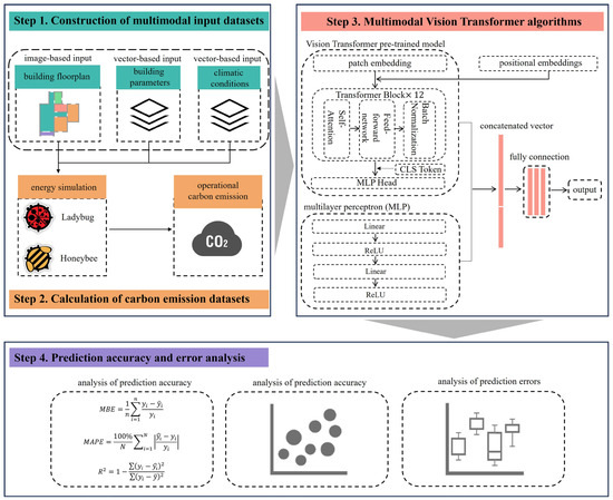
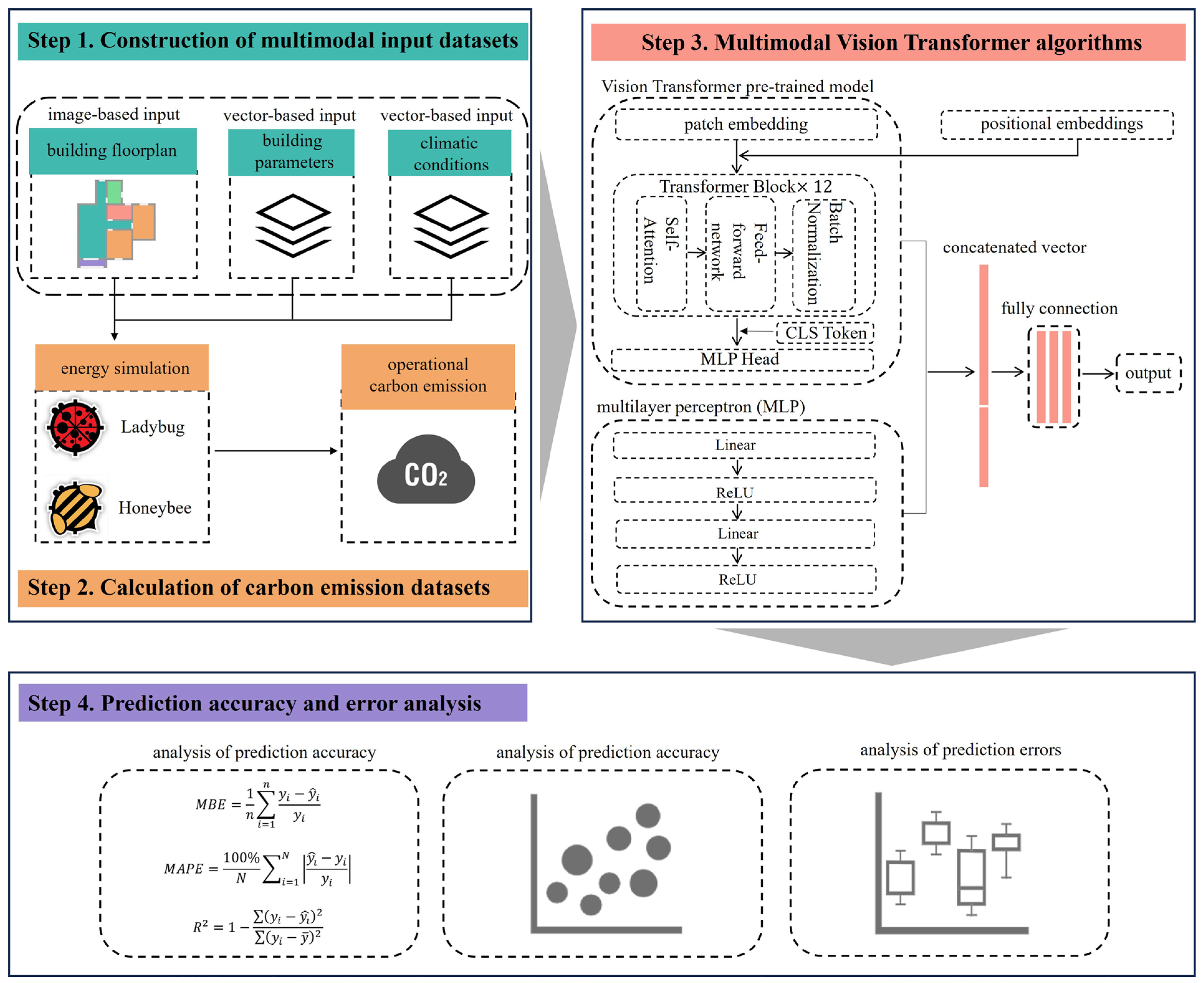
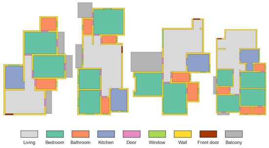
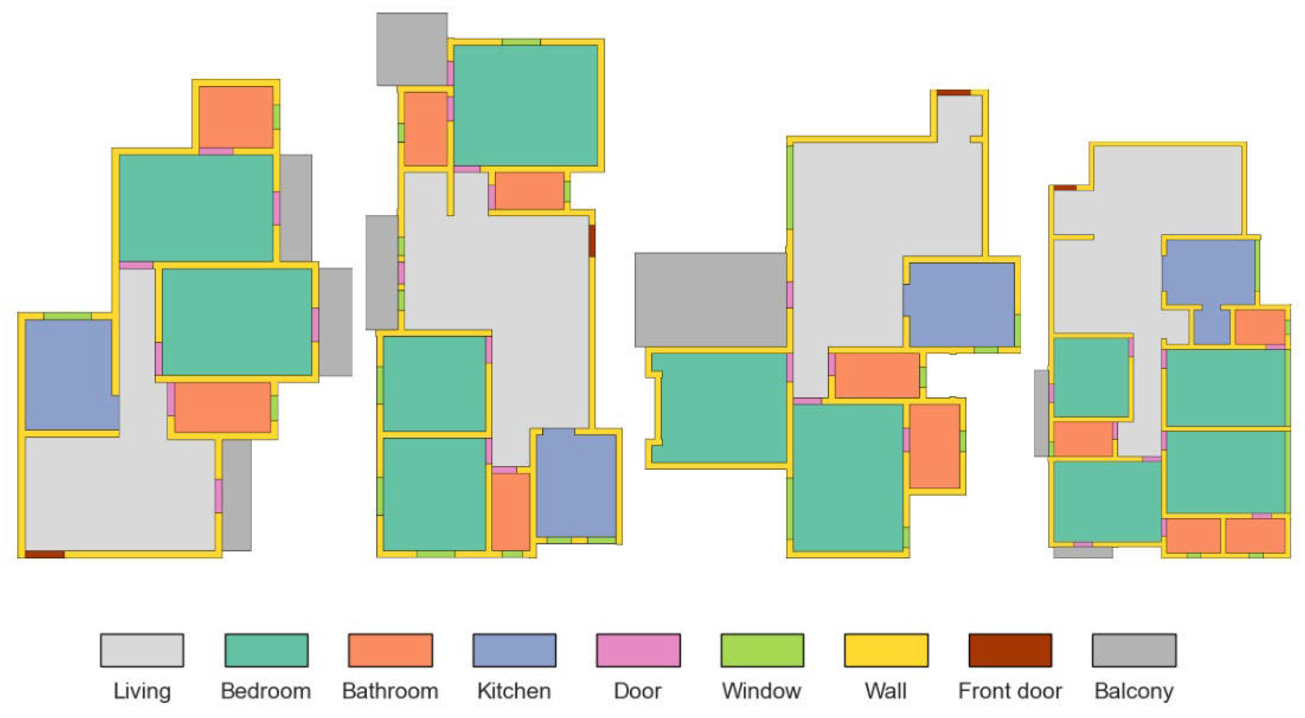
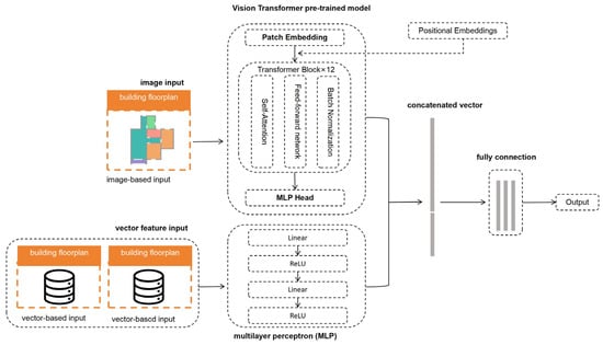
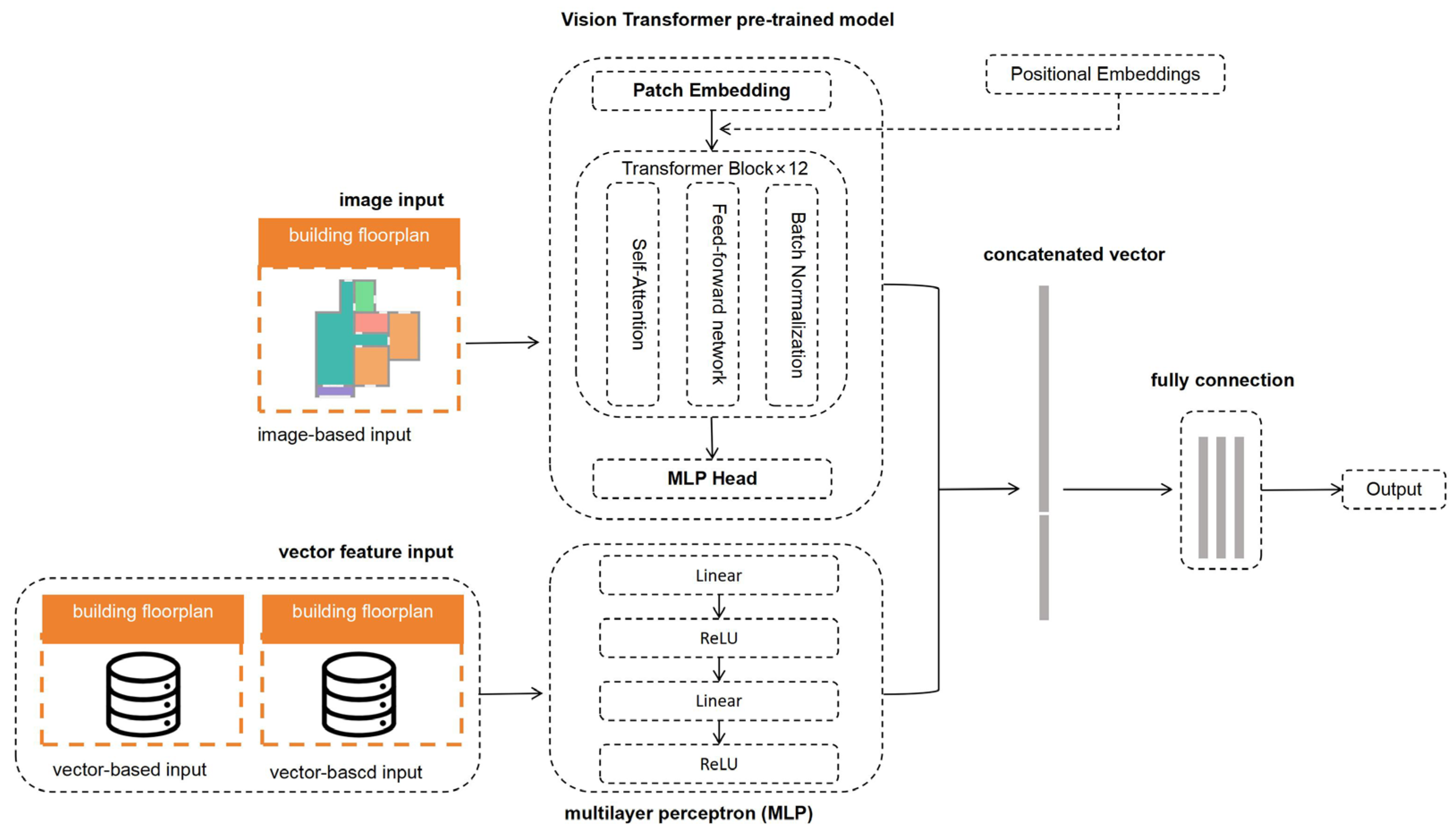
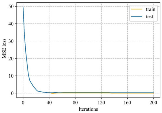
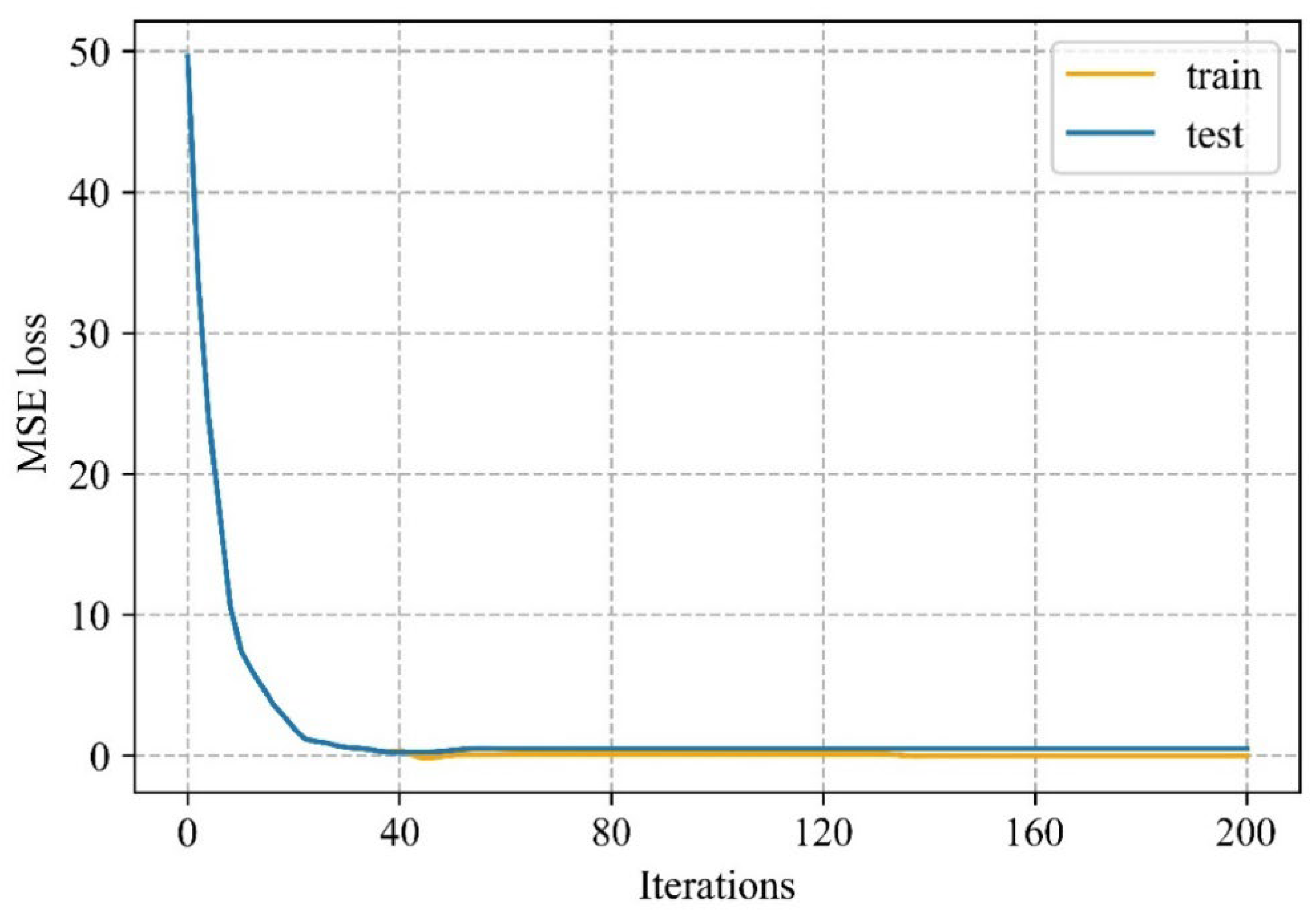
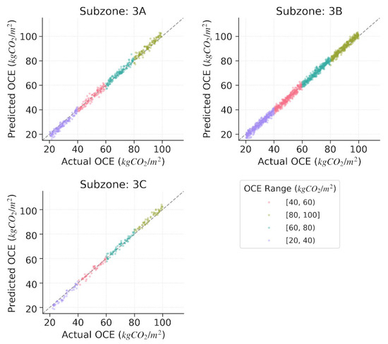
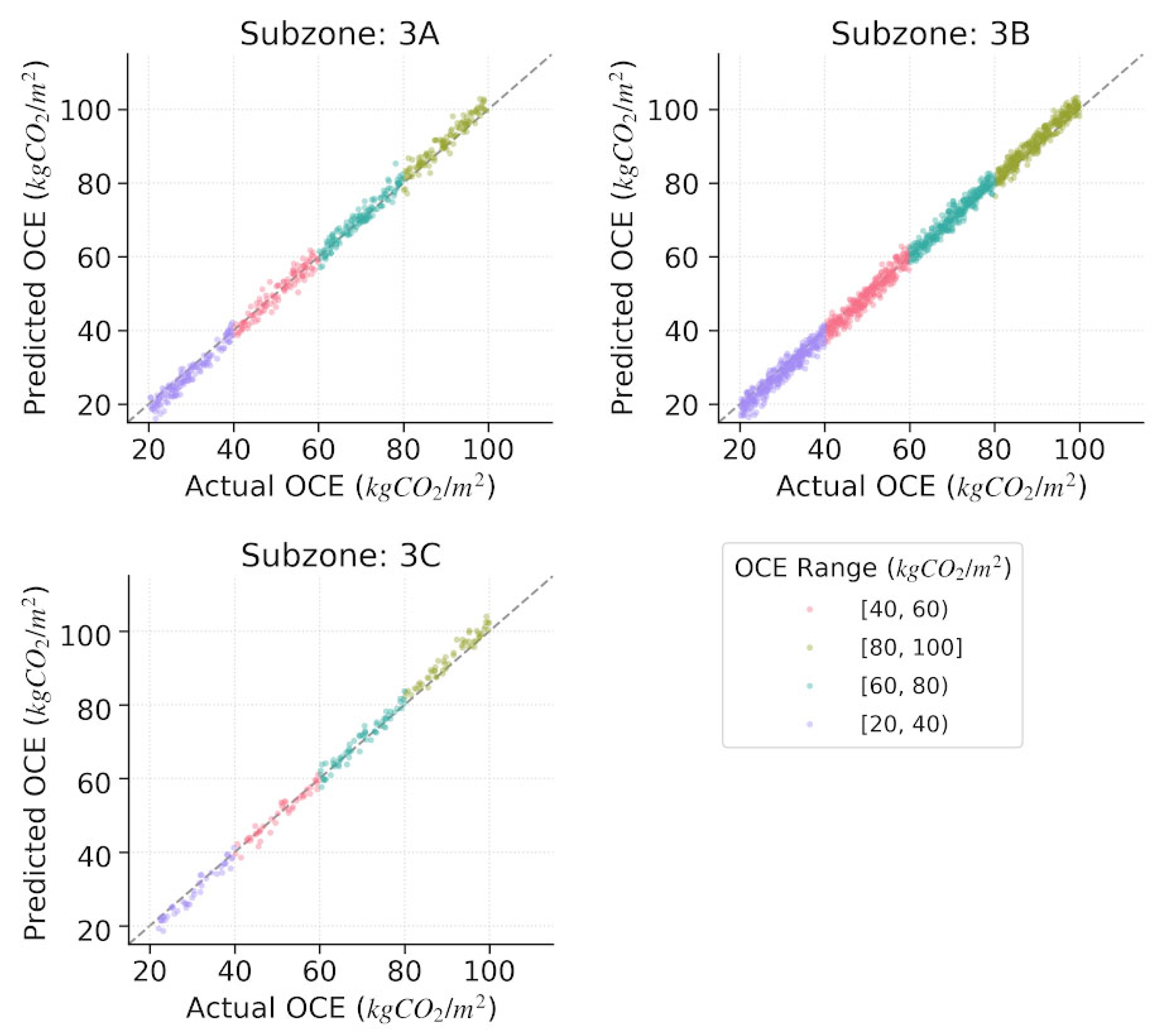
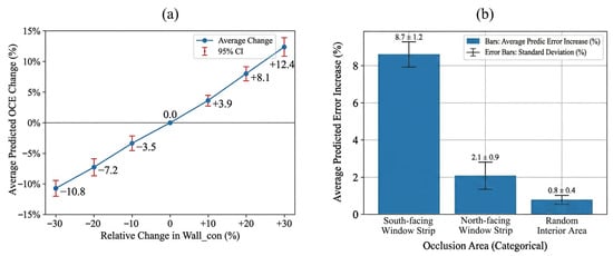
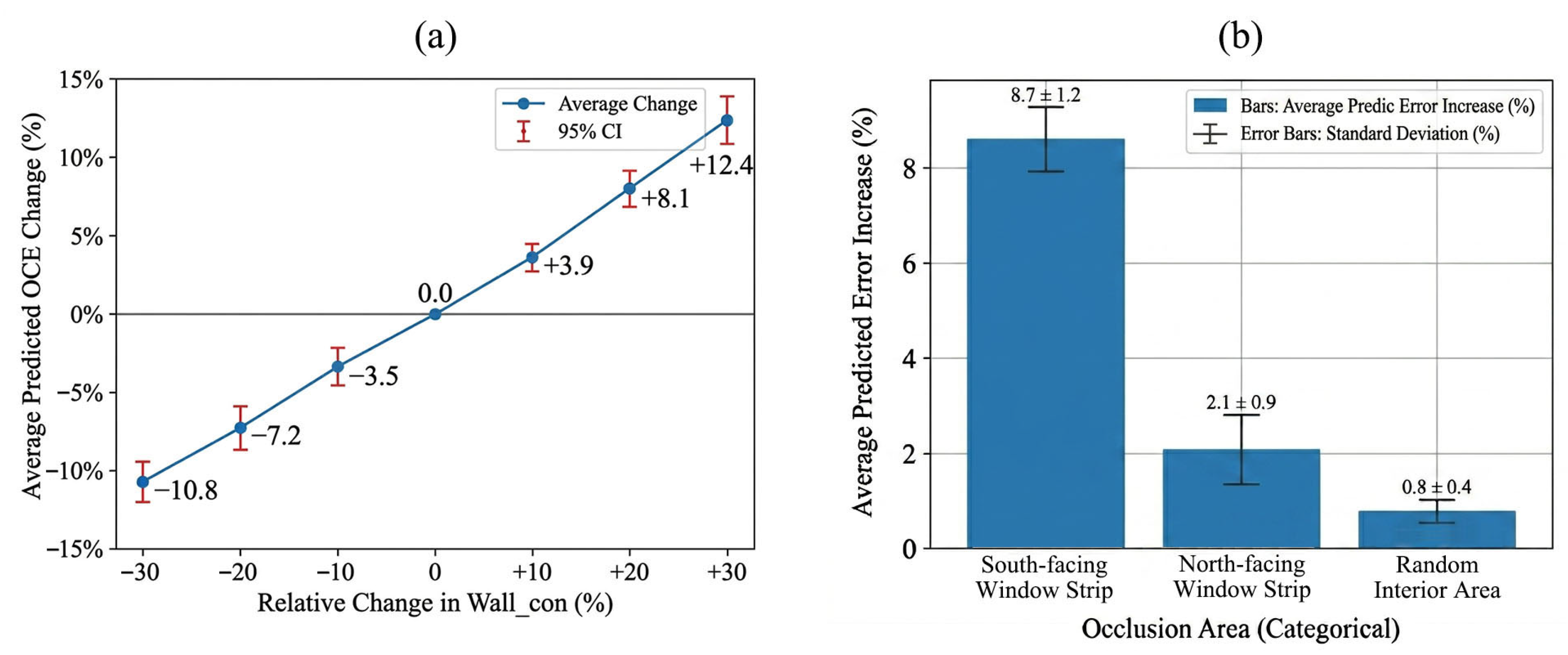















Disclaimer/Publisher’s Note: The statements, opinions and data contained in all publications are solely those of the individual author(s) and contributor(s) and not of MDPI and/or the editor(s). MDPI and/or the editor(s) disclaim responsibility for any injury to people or property resulting from any ideas, methods, instructions or products referred to in the content. |
© 2026 by the authors. Licensee MDPI, Basel, Switzerland. This article is an open access article distributed under the terms and conditions of the Creative Commons Attribution (CC BY) license.