


Abstract
Reducing carbon emissions during construction is essential for meeting dual carbon targets. Current green scheduling methods assume fixed emission factors, overlooking time-dependent variations driven by grid peak-valley patterns. Under interval duration uncertainty coupled with tight dynamic carbon budgets, conventional algorithms struggle with sparse feasible solutions and slow Pareto front convergence. We formulate a bi-objective interval RCPSP model with time-varying carbon emission factors that minimizes both interval makespan and total carbon emissions. A possibility degree measure converts scalar carbon budgets into linearized hard constraints. To solve this NP-hard problem, we propose the Knowledge-Driven Interval Multi-Objective Evolutionary Algorithm (KD-IMOEA), which integrates four components: Knowledge-Driven Initialization (KDI), Adaptive Time-window Carbon-aware Decoding (TCD), Carbon Budget-aware Repair Mutation (CBM), and Interval Pareto Elite Archive (IPA), forming an end-to-end carbon-aware optimization pipeline. We validate KD-IMOEA on J30 through J120 benchmark instances; results show it outperforms four established algorithms, including NSGA-II, in both convergence and distribution, with hypervolume (HV) gains up to 6.3%. A green building case study confirms that KD-IMOEA exploits spatiotemporal decoupling to identify float time and assign energy-intensive machinery to lower-carbon operating profiles. At the optimal compromise makespan of 169.5 days, this strategy cuts carbon emissions by 3.07% over traditional baselines, enabling management-driven emission savings without extending project duration.
1. Introduction
Construction ranks among the largest contributors to global carbon emissions. The United Nations Environment Programme [1] reports that buildings and construction consume 32% of global final energy and produce 34% of energy-related CO2 emissions, totaling a record 9.8 Gt in 2023. In China, building life-cycle emissions exceed 50% of the national total [2], largely because the construction phase relies on fossil-fuel-driven heavy machinery. China’s dual carbon targets (peaking by 2030, neutrality by 2060) and national standards GB/T 50378-2019 [3] and GB/T 51366-2019 [4] now set explicit caps on construction-phase emissions. Current emission reduction measures heavily rely on equipment upgrades and technological innovations. For instance, intelligent structural health monitoring via machine learning [5,6], along with low-carbon material substitutions like eco-friendly cementitious composites [7,8] and FRP-confined concrete members [9,10], have been widely adopted to lower embedded carbon. While these hardware and material-driven advancements significantly enhance structural performance, they leave the micro-level scheduling and sequencing of construction activities largely untapped as a management-driven emission reduction lever.
How activities are sequenced, when they start, and how resources are allocated together determine mechanical equipment intensity across time periods. Grid carbon emission factors differ markedly between peak and valley hours, with peak-period factors roughly 1.5–2.0 times the valley-period values [11]. Embedding these time-varying factors into scheduling optimization and using algorithms to assign energy-intensive activities to lower-carbon operating profiles can cut emissions through better management alone, without purchasing new equipment. In this study, such assignments are represented as start-day commitments and low-carbon operating-profile recommendations rather than deterministic hour-by-hour dispatch instructions. The detailed intra-day deployment of equipment and crews remains a tactical-layer decision made by the project team under weather, safety, labor, and regulatory constraints. This gives budget-constrained firms a practical path to satisfying both schedule targets and green certification.
This engineering need maps directly to the resource-constrained project scheduling problem (RCPSP), which assigns activity start times under precedence and renewable-resource capacity constraints to minimize makespan. RCPSP is NP-hard [12], and instances beyond small scale require metaheuristics. Multi-objective evolutionary algorithms, notably NSGA-II [13], NSGA-III [14], MOEA/D [15], and SPEA2 [16], have been applied to RCPSP variants that balance makespan against cost or resource leveling [17]. Carbon emissions have recently entered scheduling models as an additional objective. Aramesh et al. [18] added CO2 to multi-mode RCPSP under interval-valued fuzzy uncertainty. Razi and Ansari [19] combined machine learning with metaheuristics for four-way time-cost-energy-CO2 trade-offs. Rahman and Han [20] built a decarbonization-focused production scheduling framework, confirming that activity-level sequencing contributes meaningfully to emission reduction. Ding et al. [21] surveyed the past decade of RCPSP research and identified carbon optimization and uncertainty handling as two fast-growing directions.
Activity durations in construction are affected by weather, material supply, and labor availability, making precise prediction difficult at the planning stage. Uncertainty modeling has accordingly become a major branch of scheduling research. Three approaches dominate. Stochastic programming assumes durations follow known probability distributions and optimizes expected makespan or conditional value-at-risk (CVaR). Fu et al. [22] proposed a distributionally robust RCPSP model that minimizes CVaR when duration distributions are not fully known, improving schedule robustness. Stochastic methods, however, need sufficient historical data to fit distributions, and accuracy degrades when past cases are scarce or conditions differ substantially.
Fuzzy programming uses fuzzy numbers or interval-valued fuzzy numbers to capture subjective duration uncertainty. Patoghi and Mousavi [23] modeled activity duration and material ordering uncertainty with interval type-2 fuzzy numbers in a multi-project RCPSP. Fuzzy methods reduce dependence on precise distributions, but constructing membership functions still demands strong subjective judgment. Interval programming requires only optimistic and pessimistic duration bounds, representing durations as closed intervals. Hazır and Ulusoy [24] noted in their systematic review that interval methods strike a good balance between data requirements and modeling complexity, suiting construction scenarios where historical data are scarce.
Interval methods have been further validated in complex multi-objective scheduling. Ghasemi et al. [25] developed a scheduling model for time-cost-quality trade-offs that handles multi-mode resources and interval uncertainty. Hatami-Moghaddam et al. [26] built a robust multi-objective resource-constrained scheduling framework for duration fluctuations and time-window constraints. The value of embedding uncertainty in scheduling frameworks is now broadly accepted. Li et al. [27] confirmed that uncertainty modeling improves the executability of resulting schedules. Aghileh et al. [28] reviewed methods for handling uncertainty and resource flexibility in multi-project scheduling, noting that combining uncertainty modeling with multi-objective optimization remains an open research area.
Despite these advances, jointly addressing green scheduling and uncertainty under realistic dynamic constraints still faces three bottlenecks. At the modeling level, most studies assume constant carbon emission factors throughout the project cycle, ignoring time-varying characteristics from grid peak-valley structures. This static assumption breaks the link between energy-intensive machinery operations and external low-carbon windows, preventing fine-grained shift scheduling. At the algorithm level, when interval uncertainty couples tightly with stringent carbon budget constraints, the feasible search space shrinks dramatically. Standard multi-objective evolutionary algorithms such as NSGA-II rely on random initial populations and blind crossover-mutation operators with no awareness of carbon budget consumption, resulting in low initial feasibility rates and slow Pareto front convergence. At the evaluation level, interval multi-objective Pareto dominance is typically based on midpoints alone. While computationally simpler, this discards risk information carried by interval widths and cannot distinguish schedules with equal midpoint objectives but different uncertainty profiles, limiting support for risk-sensitive decisions.
To address these gaps, we introduce time-varying carbon emission factors into the uncertainty scheduling framework, formulate a bi-objective interval RCPSP under carbon constraints, and develop KD-IMOEA for efficient solution. The main contributions are as follows:
(1) We construct a bi-objective interval scheduling model with time-varying carbon emission factors. The model uses interval numbers for duration uncertainty and minimizes both interval makespan and interval total carbon emissions. We apply the possibility degree measure to link interval carbon emissions with a scalar carbon budget as a hard constraint, linearizing the nonlinear time-dependent emission calculation into precomputed matrices. This provides a rigorous framework for coupling uncertainty with green certification standards.
(2) We propose KD-IMOEA with four integrated carbon-aware components. To counter the sharp feasibility decline under tight carbon budgets, the algorithm embeds carbon awareness across four evolutionary stages: KDI raises initial population feasibility through carbon-guided construction rules; TCD biases early-stage decoding toward low-emission time periods; CBM repairs infeasible offspring by reallocating high-carbon activities to low-emission periods; IPA preserves historically optimal interval Pareto solutions in an external archive. Benchmark experiments show that KD-IMOEA consistently and significantly outperforms four baseline algorithms in both convergence and distribution uniformity.
(3) We reveal a spatiotemporal decoupling mechanism that achieves management-driven emission savings at zero hardware cost. A green building case study confirms that KD-IMOEA can identify energy-intensive activities with float time and assign them to lower-carbon operating profiles without delaying overall makespan. This micro-level asymmetric scheduling releases over 3% carbon safety margin, offering budget-constrained contractors an algorithm-driven tool for carbon compliance that reduces quota violation risk without additional equipment investment.
The remainder of this paper is organized as follows. Section 2 formulates the bi-objective interval RCPSP model. Section 3 presents KD-IMOEA and its four carbon-aware components. Section 4 reports benchmark comparisons, ablation studies, and parameter sensitivity analysis. Section 5 presents a green building case study. Section 6 discusses practical implications, applicability boundaries, and project-management workflows. Section 7 concludes the paper and outlines future research directions.
2. Problem Formulation
2.1. Problem Description
Consider a green building project consisting of construction activities, represented by an activity-on-node (AON) network . In the node set , and are virtual start and finish activities with zero duration; the arc set encodes precedence relations. If , then activity must be completed before activity starts (finish-to-start constraint). The project planning horizon is discretized into equal-length time periods, with the period set denoted as . A period is defined as the smallest temporal interval at which scheduling decisions—activity start times , resource availabilities , and emission factors —are made. Throughout this paper, a period corresponds to one working day, following the standard RCPSP convention. This day-level instantiation applies to both the benchmark experiments of Section 4 (where emission factors are parameterized at day-level resolution) and the green building case study of Section 5 (where intra-day grid-emission heterogeneity is captured at the emission-factor level via grid-category multipliers, rather than through finer temporal subdivision; see Section 5.1 for details). This unified day-level abstraction reflects the strategic-layer scope of the proposed framework: the model commits start-day decisions for each activity, while intra-day deployment of crews and equipment is determined at the tactical layer by the project team based on real-time conditions—a separation that integrates with established master-schedule workflows and is discussed in detail in Section 6.2. Activity durations are stated in calendar days throughout the paper.
The project uses types of renewable resources (tower cranes, labor crews, etc.). The available capacity of resource in period is denoted as , whose time dependence reflects external constraints such as nighttime construction bans and rainy season shutdowns. The fixed demand of activity for resource per period is denoted as . We adopt the non-preemption assumption: once an activity starts, it must be executed continuously until completion without interruption.
Construction activity durations are affected by multiple factors such as weather, material supply, and labor skill, making them difficult to predict precisely during the planning phase. We use interval numbers to characterize duration uncertainty: for activity , only the optimistic duration lower bound and pessimistic duration upper bound need to be estimated, with the interval duration:
representing the possible range of duration values. Compared to stochastic programming, interval programming does not require presetting probability distributions and has lower data requirements in scenarios where construction project historical data are limited, making it more suitable for actual engineering conditions.
According to the Standard for Carbon Emission Calculation of Buildings (GB/T 51366-2019), the carbon emission intensity of energy sources such as electricity and diesel consumed by mechanical equipment during the construction phase exhibits time dependence: the electricity carbon emission factor varies with the energy structure (renewable energy proportion) of the grid during peak and valley periods, and mechanical equipment also experiences increased carbon emissions per unit energy consumption during extreme temperature periods due to reduced thermal efficiency. To this end, we define the carbon emission factor of resource in period (unit: kgCO2e/(unitperiod)). Following the day-level period instantiation in Section 2.1, represents the day-level effective emission factor of resource on working day . In the benchmark experiments (Section 4), varies across days following a representative grid-emission profile; in the green building case study (Section 5.1), intra-day grid heterogeneity is captured by assigning each working day to one of three operating-profile categories—peak, mid-level, and valley—with corresponding day-level factors , where is the resource-specific base factor and is the grid-category multiplier (full specification in Section 5.1). The direct construction carbon emission factor for labor crews is set to zero (auxiliary energy consumption for workers’ living can be amortized into the project’s fixed carbon emission baseline and does not participate in dynamic scheduling decisions).
Activity durations are interval numbers. The actual resource occupation duration is uncertain. This leads to the total carbon emissions during the construction phase being an interval number (causal chain: uncertain ⇒ resource occupation duration uncertain ⇒ carbon emissions uncertain). The interval expression for total carbon emissions is detailed in Equation (11) in Section 2.3, denoted here as . The project has a total carbon emission quota (unit: kgCO2e) according to the three-star green building certification requirements. Since is an interval number and is a scalar, they must be compared through a possibility-based constraint: the confidence level quantifies the degree of quota satisfaction, where corresponds to the most conservative constraint (i.e., pessimistic carbon emissions do not exceed the quota), corresponds to the expected value criterion, and the interval covers the complete decision spectrum from the expected criterion to the worst-case criterion (the formal definition of possibility degree is given in Section 2.2).
We simultaneously consider two competing interval objectives: minimizing the interval project makespan and the interval total carbon emissions , forming a bi-objective interval RCPSP. Its mathematical essence is an interval bi-objective mixed-integer program. The carbon emission quota Q plays a dual role in this problem: as a hard constraint (when ), it is the qualification threshold for three-star green building certification, and exceeding it results in rejection; minimizing is lean optimization under the premise of meeting certification qualifications. The two have clearly distinguished semantics without redundancy. The complete mathematical model is established step by step in Section 2.3, and the interval Pareto dominance relation is given in Section 2.4; the main symbols are summarized in Table 1.
Table 1.
Main symbol notation.
2.2. Interval Number Theory
Definition 1
(Interval Number). Let and , then is called a closed interval number. When , it degenerates to a real number. For any interval number , define its midpoint and width respectively as follows:
which characterize the location and uncertainty degree of the interval number, respectively.
Interval arithmetic operations: Let , , , define:
The above operations maintain degeneration consistency with real number arithmetic, and the results remain valid interval numbers.
Definition 2
(Possibility Degree). For interval numbers and , define the possibility degree that does not exceed as follows:
when (both degenerate to real numbers), stipulate if -; otherwise 0.
Proposition 1
(Basic Properties of Possibility Degree).
- (1)
- Boundedness: ;
- (2)
- Complementarity: ;
- (3)
- Degeneration consistency: when and both degenerate to real numbers, Equation (6) reduces to standard real number comparison;
- (4)
- Neutral criterion: .
Property (2) ensures the consistency of possibility degree judgments and avoids contradictory rankings; property (4) indicates that corresponds to the expected value decision criterion based on midpoints, while corresponds to the conservative criterion under the worst-case scenario, which is fully consistent with the engineering semantics of in Section 2.1. It should be noted that the possibility degree in this paper is exclusively used to support the linearization derivation of constraint (C4) (see Equation (16) in Section 2.3), while the dominance relation between interval objectives is independently defined by the upper and lower bound comparison criterion in Section 2.4, and the two are not mixed.
2.3. Mathematical Model
2.3.1. Decision Variables and Derived Variables
The core of scheduling decisions is to determine the start period of each activity. From Table 1, is a binary decision variable, and the deterministic start period of activity is as follows:
is a linear derived quantity of , uniquely determined by the decision. Equation (7) is a definitional equality rather than an independent constraint; for brevity, subsequent constraints use to replace , and the two are completely equivalent. Uncertainty only originates from the interval duration . We stipulate that an activity starts at the beginning of period , occupies periods , and completes at the end of period , i.e., the completion time instant is . From Equation (3), the interval completion time of activity is as follows:
2.3.2. Objective Functions
Objective one: Minimize interval project makespan
From Equation (5), taking the interval maximum over all activity interval completion times:
Objective two: Minimize interval total carbon emissions
Activity , starting in period , continuously occupies resource (with demand ) during consecutive periods , generating carbon emissions. Since , precompute the carbon emission parameters for activity starting in period t under optimistic and pessimistic durations respectively:
Both and are precomputed constant matrices depending on input data, independent of decision variables. By introducing the precomputed constant matrices and , we linearize the originally nonlinear time-dependent carbon emission calculation into a first-order linear expression with respect to , significantly reducing the model’s solution complexity while retaining complete information on time-varying carbon factors. From the interval addition in Equation (3), the interval total carbon emissions are as follows:
Both objective functions are linear interval functions with respect to , and their optimization meaning is defined by the interval Pareto dominance relation in Section 2.4.
2.3.3. Constraints
(C1) Scheduling completeness constraints: Each activity starts exactly once, and the start period is limited to the feasible window calculated by the critical path method (based on optimistic duration ):
xjt = 0, ∀ t ∉ ESj, LSj, ∀ j∈N
(C2) Precedence constraints: If , to ensure that the precedence relation still holds under the worst-case scenario (activityduration reaches pessimistic value ), the constraint takes a conservative form:
This treatment is consistent with constraint (C3) pessimistic duration assumption for resources, ensuring that the generated baseline schedule has full robustness over the entire realization range of interval durations.
(C3) Renewable resource constraints: We use pessimistic duration to construct resource constraints to ensure that resources are not overloaded under the worst-case scenario. Activity is in execution state during period if and only if it starts in some period within , thus:
The time-varying nature of uniformly covers situations such as nighttime construction bans (setting ) and rainy season load reduction, without requiring additional handling.
(C4) Carbon emission quota possibility constraint: Require that the interval carbon emissions satisfy the quota with confidence level , i.e., . Treating as a degenerate interval (, ), substituting into Equation (6) and expanding, this simplifies to the equivalent linear constraint:
Equation (16) has intuitive engineering semantics: when , it degenerates to pessimistic carbon emissions not exceeding the quota (), which is the most conservative constraint; when , it degenerates to expected carbon emissions not exceeding the quota. The continuous adjustment of λ allows decision makers to trade off between conservatism and feasible region looseness without modifying the model structure; the dual role of carbon quota and objective function has been clearly distinguished in Section 2.1.
(C5) Variable domain constraints:
2.3.4. Complete Model Summary
Integrating Equations (9)–(17), the bi-objective interval RCPSP model in this paper is as follows:
s.t. (C1) Equations (12) and (13): Scheduling completeness constraints
(C2) Equation (14): Precedence constraints (pessimistic robust)
(C3) Equation (15): Time-varying resource capacity constraints (pessimistic robust)
(C4) Equation (16): Carbon emission quota possibility constraint
(C5) Equation (17): Variable domain constraints
Model (P) contains binary decision variables, with constraint scale . It can be proven to belong to the NP-hard class by reduction from the standard RCPSP NP-hardness, and the exact solution is only suitable for small-scale instances.
2.4. Interval Pareto Dominance
Definition 3
(Interval Pareto Dominance). Let be the interval objective value of solution on objective . For two feasible solutions and of model (P), Pareto-dominates in the interval sense (denoted ) if and only if for all objectives :
and at least one objective exists such that one of the above inequalities holds strictly ().
This definition simultaneously constrains the optimistic case (lower bound) and pessimistic case (upper bound), naturally favoring solutions with smaller interval widths, i.e., better objective values with lower uncertainty. Compared to weak dominance criteria that only compare midpoints, this definition completely preserves the risk information carried by interval widths, consistent with the original intention of introducing interval durations in this paper.
Definition 4
(Interval Pareto Optimal Solution Set and Front). Let be the set of all feasible solutions, define:
as the interval Pareto optimal solution set, and its corresponding objective vector set is called the interval Pareto front. The goal of the algorithm in this paper is to approximate .
2.5. Constraint Handling
During the optimization process of evolutionary algorithms, candidate solutions may violate constraint (C4). To establish a unified comparison criterion between feasible and infeasible solutions, define the constraint violation degree (VD) of solution as follows:
if and only if x satisfies constraint (C4), and reflects the relative degree of carbon exceeding the quota.
Based on this, solution comparison follows the feasibility-first rule: If and , then u is superior to v; if , then the one with smaller VD is preferred; if , compare according to the interval Pareto dominance relation in Definition 3.
Since model (P) adds interval uncertainty, time-varying emissions, and dynamic quotas to the already NP-hard RCPSP, exact methods are viable only for tiny instances. Section 3 therefore develops the KD-IMOEA metaheuristic, which directly embeds the feasibility-first rule established above into its non-dominated sorting mechanism.
3. Algorithm Design
3.1. Overall Framework
Since model (P) is NP-hard (Section 2), exact methods are computationally infeasible for medium- and large-scale instances. We propose KD-IMOEA, building on the NSGA-II framework. Targeting three structural features of model (P), interval duration uncertainty, time-varying emission factors, and possibility-based carbon budget constraints, the algorithm embeds domain knowledge into four evolutionary stages: initialization, decoding, mutation, and archive management. These map to four components: Carbon-aware Knowledge-Driven Initialization (KDI, Section 3.2), Adaptive Time-window Carbon-aware Decoding (TCD, Section 3.3), Carbon Budget-aware Repair Mutation (CBM, Section 3.4), and Interval Pareto Elite Archive (IPA, Section 3.5). The algorithm applies the interval Pareto dominance from Definition 3 for solution comparison and the feasibility-first rule from Section 2.5 for constraint handling, outputting an approximate interval Pareto front .
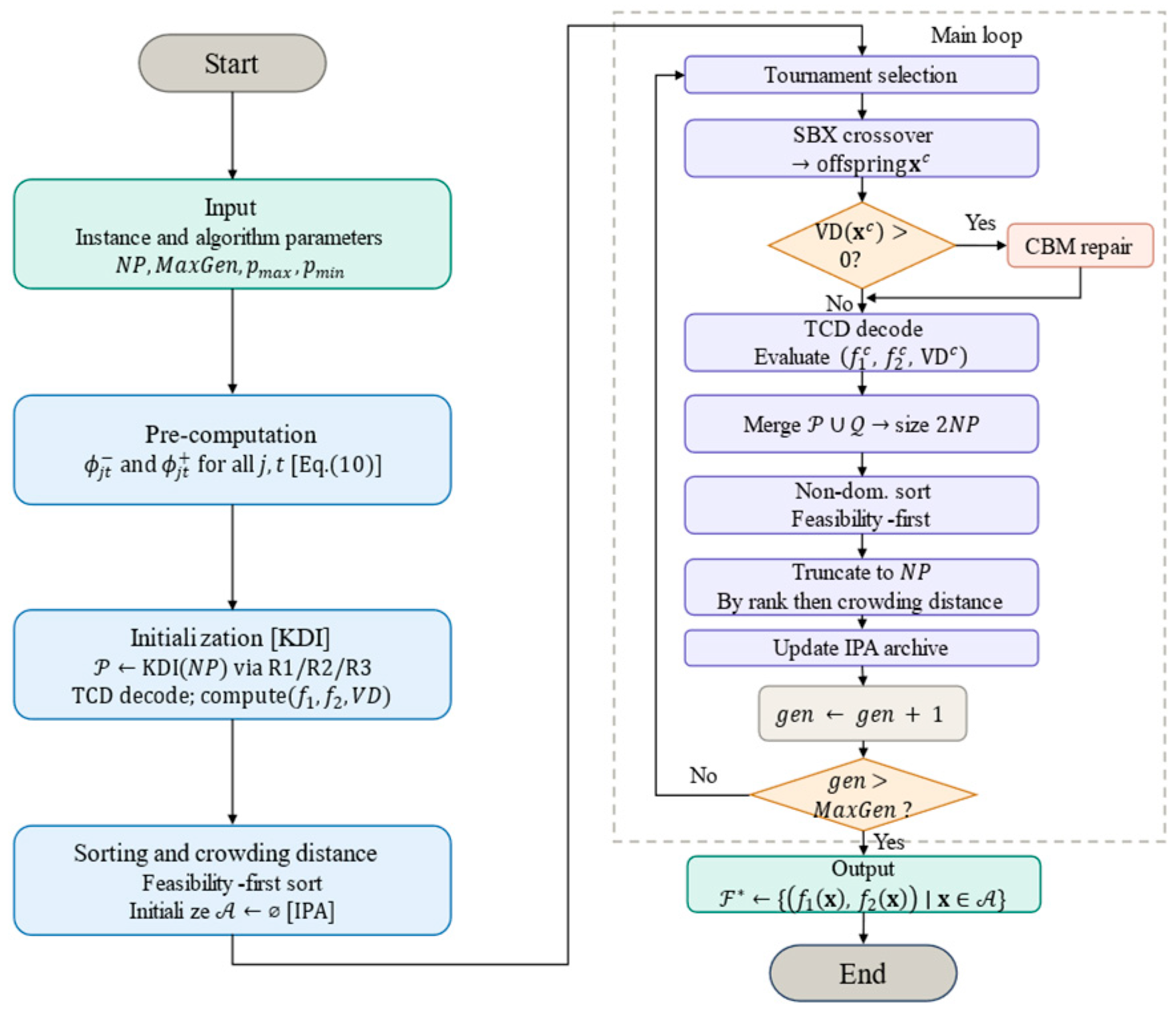
The overall flow is shown in Figure 1, with complete pseudocode in Algorithm 1. Execution has three phases: precomputation, initialization, and main loop. During precomputation, emission parameter matrices - and are built once via Equation (10) and reused by all subsequent decoding and constraint evaluation. During initialization, KDI generates the initial population using three domain-specific rules, TCD decodes individuals, feasibility-first non-dominated sorting is performed, and the IPA archive A is initialized empty. In the main loop, each generation runs binary tournament selection, SBX crossover, and TCD decoding. When an offspring violates the carbon budget (), CBM repair is triggered. Parent and offspring populations are merged, sorted by feasibility-first non-dominated sorting, and truncated to NP individuals; the IPA archive is then updated. The loop terminates at gen > MaxGen, outputting the non-dominated set F* from the archive. Overall time complexity is , the same order as standard NSGA-II.
Figure 1.
Flowchart of KD-IMOEA.
| Algorithm 1 KD-IMOEA |
| Input: Project instance ; algorithm parameters , , , |
| Output: Approximate interval Pareto front |
| //Pre-computation |
| 1: for all , do compute and via Equation (10) end for |
| //Initialization |
| 2: KDI Algorithm 2, Section 3.2 |
| 3: for to do |
| 4: TCD-Decode Algorithm 3, Section 3.3 |
| 5: end for |
| 6: Perform feasibility-first non-dominated sorting on ; compute crowding distances |
| 7: ; IPA-Update non-dominated Algorithm 5, Section 3.5 |
| //Main loop |
| 8: for to do |
| 9: |
| 10: for to do |
| 11: Select parents , via binary tournament selection |
| 12: SBX-Crossover |
| 13: if then |
| 14: CBM-Repair Algorithm 4, Section 3.4 |
| 15: end if |
| 16: TCD-Decode |
| 17: |
| 18: end for |
| 19: Combined population, size |
| 20: Perform feasibility-first non-dominated sorting on ; compute crowding distances |
| 21: Select top individuals from by rank, then crowding distance |
| 22: IPA-Update non-dominated Algorithm 5, Section 3.5 |
| 23: end for |
| //Output |
| 24: return |
3.2. Carbon-Aware Knowledge-Driven Initialization (KDI)
Population initialization quality directly affects convergence speed and solution diversity. Embedding domain knowledge into initial population generation using a multi-rule hybrid strategy can markedly improve initial quality and accelerate convergence [29]. For model (P), purely random initialization is blind to the carbon budget constraint (C4), producing many infeasible individuals and increasing the computational burden of subsequent repair and evolution. KDI embeds the precomputed emission matrices and along with resource utilization data into population generation. Based on the Serial Schedule Generation Scheme (SSGS) [30], KDI produces an initial population of size by mixing three construction rules R1, R2, and R3 at ratios 40%, 30%, and 30%. The full procedure is in Algorithm 2.
Rule R1 (40%): Carbon-oriented construction. For each activity, compute its carbon intensity , where is the time-averaged emission factor for resource . Sort activities by descending , and assign each to the lowest-emission time satisfying precedence and resource feasibility. R1 uses the precomputed matrix to steer carbon-intensive activities toward low-emission periods, raising the initial population’s feasibility rate for constraint (C4).
Rule R2 (30%): Resource-oriented construction. Sort activities by descending total resource demand , and assign each to the feasible period with lowest current resource utilization , alleviating scheduling congestion while satisfying (C3). R2 complements R1: R1 targets carbon, R2 targets resource balance, and together they improve feasibility.
Rule R3 (30%): Random construction. Randomly generate topological sequences satisfying (C1)–(C2), injecting diversity to prevent the greedy strategies of R1 and R2 from concentrating the initial population in local regions.
All individuals from R1-R3 are decoded by TCD (Section 3.3), mapped to interval schedules, and evaluated for , then passed to feasibility-first non-dominated sorting in line 6 of Algorithm 1.
| Algorithm 2 Carbon-Aware Knowledge-Driven Initialization (KDI) |
| Input: Project instance ; population size ; precomputed , |
| Output: Initial population |
| //R1: emission-guided construction (40% of NP) |
| 1: for to do |
| 2: Rank activities by carbon intensity in descending order |
| 3: for each activity in ranked order do |
| 4: subject to precedence and resource feasibility |
| 5: Assign |
| 6: end for |
| 7: resulting schedule; |
| 8: end for |
| //R2: resource-guided construction (30% of NP) |
| 9: for to do |
| 10: Rank activities by resource demand in descending order |
| 11: for each activity in ranked order do |
| 12: subject to precedence and resource feasibility |
| 13: Assign |
| 14: end for |
| 15: resulting schedule; |
| 16: end for |
| //R3: random construction (remaining 30% of NP) |
| 17: for to do |
| 18: random topological ordering satisfying constraints (C1)–(C2) |
| 19: |
| 20: end for |
| 21: return |
3.3. Adaptive Time-Window Carbon-Aware Decoding (TCD)
The decoder maps chromosomes (priority lists) to feasible interval schedules and computes objective values and constraint violation degrees. It is the bridge between population evolution and schedule evaluation. TCD is called in line 4 of Algorithm 1 (initialization) and line 16 (offspring evaluation); its output triplet implements Equations (9), (11) and (20).
Chromosome representation and basic decoding. We use an activity list (priority list) as chromosome encoding, where activities satisfy topological feasibility (all predecessors precede each activity). Basic decoding follows SSGS [31]: activities are processed in priority-list order and each is scheduled at the earliest feasible start period satisfying (C1)–(C3). This guarantees resource and precedence feasibility.
Carbon-aware extension: Pure SSGS ignores differences between periods, often producing high-carbon solutions under time-varying factors. TCD adds carbon-aware decision-making within the feasible window of basic SSGS: with adaptive probability , the activity is placed in the period that minimizes the resource-weighted emission load ; with probability , the earliest-start strategy is retained, where
This probability starts high (), to guide the population toward low-carbon feasible regions, then decays to , preserving makespan optimization space and preventing excessive carbon bias that would reduce diversity [32]. At (initialization stage), , consistent with the KDI carbon-aware orientation. The decoding data flow is shown in Figure 2: the priority list is expanded by SSGS into time-window heat bars, probability drives a two-branch decision, the Yes branch selects lowest-EF period , the No branch retains , and both converge through to complete schedule assignment and objective evaluation.
Figure 2.
TCD decoding mechanism: adaptive carbon-aware time-period selection.
Objective and constraint evaluation. After activity placement, the precomputed matrices and (line 1 of Algorithm 1, Equation (10)) linearly compute interval total emissions; Equation (9) gives interval makespan; the objective vector and VD from Equation (20) are obtained. When VD > 0, CBM repair is triggered (line 13 of Algorithm 1). When VD = 0, the individual enters non-dominated sorting directly. The complete process is in Algorithm 3.
| Algorithm 3 Adaptive Time-window Carbon-aware Decoding (TCD) |
| Input: Chromosome (priority list) ; generation counter ; parameters , , ; precomputed , ; instance |
| Output: Interval objective tuple |
| //Adaptive carbon-aware probability |
| 1: |
| //Serial schedule generation (SSGS) with carbon-aware time-period selection |
| 2: Initialize resource usage for all , |
| 3: for each activity in priority-list order do |
| 4: Determine feasible window based on constraints (C1)–(C2) and current |
| 5: Draw |
| 6: if then |
| 7: Carbon-aware: lowest-EF period |
| 8: else |
| 9: Standard SSGS: earliest feasible start |
| 10: end if |
| 11: Set ; update for |
| 12: end for |
| //Evaluate interval objectives and constraint violation |
| 13: Equation (9) |
| 14: Equation (11) |
| 15: Equation (20) |
| 16: return |
3.4. Carbon Budget-Aware Repair Mutation (CBM)
SBX crossover is blind to the carbon budget constraint (C4), and offspring frequently violate it . Penalty functions require manual coefficient tuning with high sensitivity. Discarding infeasible solutions wastes crossover computation. CBM, triggered conditionally in lines 13–14 of Algorithm 1, combines repair and mutation: it restores feasibility while directly cutting emissions, achieving both constraint satisfaction and objective improvement in synergy with the feasibility-first rule (Section 2.5).
Step 1: Identify high-carbon activities. For infeasible offspring , compute the carbon contribution of each activityusing the weighted parameters from Equation (16):
Sort by descending and select the top 30% as the high-carbon set . This step reuses the precomputed matrix (line 1 of Algorithm 1, Equation (10)) with no additional overhead.
Step 2: Lowest-EF period reallocation. For each activity in , search within for periods satisfying (C1)–(C3), select minimizing , and reassign. This strategy mirrors KDI rule R1 (Section 3.2) and the TCD carbon-aware branch (Section 3.3), reflecting internal consistency across algorithm components. Figure 3 illustrates the repair: high-carbon activities , , initially in high-emission periods (orange, ↑) are moved to lowest-EF periods within their windows (green, ↓), recovering from VD > 0 to VD = 0.
Figure 3.
CBM repair mechanism.
Step 3: Update. After reallocation, update the resource matrix . The repaired offspring returns to line 16 of Algorithm 1 for TCD re-evaluation. If persists after repair, the feasibility-first rule automatically downgrades it in sorting without re-triggering CBM, preventing infinite loops. The complete procedure is in Algorithm 4.
| Algorithm 4 Carbon Budget-aware Repair Mutation (CBM) |
| Input: Infeasible offspring with ; precomputed , ; parameters , ; instance |
| Output: Repaired offspring |
| //Step 1: Identify high-carbon activities |
| 1: for all do |
| 2: Equation (22) |
| 3: end for |
| 4: top activities ranked by descending |
| //Step 2: Reassign to lowest-emission feasible periods |
| 5: for each do |
| 6: subject to (C1)–(C3) |
| 7: Set ; clear for all |
| 8: Update for |
| 9: end for |
| //Step 3: Return repaired offspring |
| 10: return Re-evaluated by TCD, Algorithm 1 Line 16 |
3.5. Interval Pareto Elite Archive (IPA)
Standard NSGA-II elite preservation is tied to within-population non-dominated sorting, and each generation’s truncation inevitably discards some historical high-quality solutions; therefore, the final output reflects only the last generation’s local optimum rather than the global optimum across all generations. IPA addresses this as an external archive independent of the evolving population, maintaining the non-dominated set discovered throughout execution and ensuring the output front covers the entire search history. IPA is initialized as in line 7 of Algorithm 1 and updated in line 22 of each generation. The complete procedure is in Algorithm 5.
Filtering. Each candidate from (current population’s non-dominated individuals) undergoes bidirectional filtering via Definition 3: if any dominates (), is discarded; otherwise, all solutions in dominated by are removed and is added. This strictly follows the upper/lower bound comparison, preserving interval width information.
Capacity control. Archive capacity is . When , individuals with the smallest crowding distance are deleted until , maintaining distribution uniformity in objective space.
Elite injection. After each update, elites randomly selected from replace equal individuals with the smallest crowding distance in , reintroducing historical optima to prevent genetic drift.
Upon termination, the objective vectors of all individuals in form the output returned in line 24 of Algorithm 1, closing the KD-IMOEA flow.
| Algorithm 5 Interval Pareto Archive Update (IPA-Update) |
| Input: Archive ; candidate set (non-dominated individuals from current population); population ; archive capacity |
| Output: Updated archive |
| //Step 1: Filter and update archive via interval Pareto dominance |
| 1: for each do |
| 2: if such that then |
| 3: Discard is dominated by archive member, reject |
| 4: else |
| 5: Remove all with dominates, purge inferior members |
| 6: |
| 7: end if |
| 8: end for |
| //Step 2: Capacity control via crowding distance pruning |
| 9: if then |
| 10: Compute crowding distances for all |
| 11: Remove individuals with the smallest crowding distance until |
| 12: end if |
| //Step 3: Elite injection into population |
| 13: randomly sample individuals from |
| 14: Replace individuals with the smallest crowding distance in with |
| 15: return |
3.6. Algorithm Parameter Calibration
KD-IMOEA has four parameters: population size , maximum generations , and TCD carbon-aware probability bounds and (Equation (21)). We calibrate these using the Taguchi orthogonal experiment method [33] to avoid expensive one-at-a-time tuning.
Parameter levels. The parameter levels in Table 2 were selected based on problem scale and literature ranges [34], aiming to cover the typical operating range of population-based evolutionary algorithms while reflecting the computational scale of the proposed interval RCPSP. The population size levels represent small, medium, and relatively large populations under the same decoding cost. balances convergence opportunity and computational burden. The upper carbon-guidance probability tests moderate to fully carbon-oriented early-stage decoding, whereas controls the retained carbon bias in later generations. Thus, the Taguchi design was intended to identify a robust accuracy-efficiency trade-off rather than simply select the single run with the highest observed HV.
Table 2.
Parameter levels for Taguchi orthogonal experiment.
Orthogonal design. The array arranges nine independent runs covering main effects of four factors at three levels, reducing the 81 runs of full factorial. Hypervolume (HV) [35] serves as the performance metric: larger HV indicates better convergence and diversity [36]. Each combination is run 15 times on standard instances, with mean HV as the measure. The resulting L9 orthogonal experimental design and the corresponding mean HV values are summarized in Table 3.
Table 3.
Taguchi L9(34) orthogonal experiment results.
The total time complexity is . Per-generation overhead consists of non-dominated sorting () and the carbon-aware decoding/repair operations within TCD and CBM (). When , the component overhead is dominated by the sorting term and the asymptotic complexity matches standard NSGA-II ; this regime applies to small-scale instances and many practical engineering scenarios. For medium-scale instances such as J30 (, comparable to , hence borderline) and J60 ( with ), the component overhead begins to contribute non-negligibly. For larger instances such as J120 (), the component overhead is not absorbed by the sorting term and contributes a measurable additive cost, as quantified by the runtime comparison reported in Section 4.2.
4. Computational Experiments
4.1. Experimental Setup
Benchmark instances. The benchmark instances are constructed by augmenting the widely used PSPLIB J30, J60, and J120 RCPSP benchmark instance sets [37], which provide the original AON precedence networks, nominal activity durations, renewable-resource capacities, and baseline resource demands. For each scale, ten PSPLIB instances are selected, corresponding to 30, 60, and 120 non-dummy activities, respectively. The nominal PSPLIB duration is used as the optimistic duration , and the pessimistic duration is generated as , consistent with the interval width coefficient . The four renewable resources are mapped to construction resources: represent mechanical resources with nonzero time-varying carbon emission factors, whereas represent labor resources with . The benchmark emission-factor time series follows the same day-level peak/mid/valley operating-profile structure described in Section 2.1 and Section 5.1, using multipliers 1.2, 1.0, and 0.7 applied to resource-specific base emission factors. For each PSPLIB-derived instance, the carbon budget is dynamically calibrated by generating 100 random feasible topological schedules and setting to 85% of the median pessimistic carbon emission, thereby producing a tight but feasible carbon constraint under Equation (16). The selected PSPLIB instance IDs, emission-factor category seeds, and algorithm random seeds are fixed across all algorithms to ensure paired-comparison validity and reproducibility.
Baseline algorithms. KD-IMOEA is compared with four algorithms: NSGA-II [13], NSGA-III [14], MOEA/D [15], and SPEA2 [16]. All five share the same interval Pareto dominance (Definition 3), SSGS decoding, and order crossover (OX), ensuring that performance differences stem solely from KD-IMOEA four components (KDI, TCD, CBM, IPA).
Performance metrics. (1) Hypervolume (HV): volume dominated by the approximate front; larger is better. Reference point is 1.1× the maximum objective value across all algorithms per instance. (2) Inverted Generational Distance (IGD) [38]: average distance from reference front to approximate front; smaller is better. Reference front is the merged non-dominated set from all algorithms. (3) Spacing: distribution uniformity; smaller is better. For performance evaluation, HV, IGD, and Spacing are computed using the midpoint representation of interval objective values, and , to maintain comparability with standard multi-objective scheduling benchmarks. This midpoint-based metric calculation is used only for external evaluation; during evolutionary selection, KD-IMOEA still applies the interval Pareto dominance relation in Definition 3, which compares both lower and upper bounds of the interval objectives. Fronts are deduplicated before metric calculation.
Parameter. Taguchi-calibrated (Section 3.6): , , . Baseline (J30, J60), increased to 500 for J120. , IPA elite injection ratio 5%, CBM trigger threshold VD > 0.05. All baselines use NP = 100 and matching MaxGen.
The Wilcoxon signed-rank test () evaluates pairwise differences between KD-IMOEA and each baseline algorithm. For each scale, the mean metric value over 10 independent runs on the same instance is used as one paired observation, yielding 10 paired observations per algorithm-scale-metric comparison. To quantify the magnitude of improvement, Cohen’s is calculated from the paired improvement differences, where positive values indicate better performance of KD-IMOEA. For HV, the paired difference is defined as KD-IMOEA minus the baseline; for IGD, it is defined as the baseline minus KD-IMOEA because smaller IGD is better. Holm-Bonferroni correction is applied across all 24 pairwise comparisons.
Environment. Python 3.10, Intel Xeon Platinum 8470Q (25 cores), 90 GB RAM. Each algorithm runs 10 times per instance with different random seeds.
4.2. Benchmark Comparison Results
Table 4 and Table 5 report HV and IGD means and standard deviations for the five algorithms on J30, J60, and J120 instances (best values in bold). Figure 4 and Figure 5 show box plots. Table 6 gives the Wilcoxon test results.
Table 4.
Comparison of HV (mean ± std) across different problem scales. Bold values indicate the best performance.
Table 5.
Comparison of IGD (mean ± std) across different problem scales. Bold values indicate the best performance.
Figure 4.
Box plots of HV values for J30, J60, and J120 instances.
Figure 5.
Box plots of IGD values for J30, J60, and J120 instances. The circular markers indicate outliers.
Table 6.
Statistical test results of KD-IMOEA versus comparison algorithms. Positive Cohen’s indicates better performance of KD-IMOEA. Holm-adjusted p-values are corrected across 24 pairwise comparisons.
HV. KD-IMOEA achieves the best HV mean at all three scales. On J30, the KD-IMOEA HV is 458,540.30, leading SPEA2 (435,612.69) by ~5.3%; the J30 box plot (Figure 4) confirms both median and upper quartile exceed all baselines. On J60, the KD-IMOEA HV is 342,924.78, leading NSGA-II (325,971.38) by ~5.2%, with the most compact box indicating stable cross-instance performance. On J120, the KD-IMOEA HV is 88,757.32, leading SPEA2 (83,513.31) by ~6.3% and MOEA/D (64,731.12) by ~37.1%; the J120 box sits above all baselines. The 5–6% lead across scales peaks at 6.3% on J120, indicating that carbon-aware search provides more effective guidance in larger search spaces.
IGD. KD-IMOEA achieves the lowest IGD at all scales, confirming convergence quality. On J30: 15.34, improving 31.1% over SPEA2 (22.27). On J60: 20.72, improving 32.3% over SPEA2 (30.60). On J120: 102.74, improving 30.0% over NSGA-III (146.86). Figure 5 shows the KD-IMOEA box is consistently the lowest, with the J120 gap most pronounced. The IGD lead (30–32%) substantially exceeds the HV lead (5–6%), indicating that TCD carbon-aware decoding is particularly effective at improving convergence.
To examine dynamic search behavior, Figure 6 shows HV convergence curves on J60. KD-IMOEA achieves the highest final HV (Gen = 300) and maintains a pronounced dynamic advantage throughout evolution. Thanks to KDI, the KD-IMOEA HV starting point at Gen = 0 is markedly higher than all randomly initialized baselines. Guided by TCD, it then climbs steeply; around generation 50, the KD-IMOEA HV already approaches or exceeds some baselines’ final convergence after 300 generations (see the vertical annotation in Figure 6). At Gen = 50, the KD-IMOEA HV exceeds NSGA-II by approximately 27.1%, an early advantage attributable to the KDI high-quality initial population. This “high start, fast convergence” dynamic demonstrates the efficiency of the proposed components in accelerating convergence and explains why KD-IMOEA achieves substantial metric advantages under limited computational budgets.
Figure 6.
Convergence profiles of mean HV for the five algorithms on the representative J60 instances.
Statistical tests. As shown in Table 6, KD-IMOEA significantly outperforms all four baseline algorithms on both HV and IGD across J30, J60, and J120. All 24 Wilcoxon signed-rank tests yield positive results for KD-IMOEA, with no “−” or “≈” outcomes. After Holm-Bonferroni correction across 24 pairwise comparisons, all adjusted p-values remain below the 0.05 significance threshold, indicating that the statistical significance remains valid after multiple-comparison correction. The positive Cohen’s values further indicate that the improvements are not only statistically significant but also practically meaningful. The largest effect sizes are observed against MOEA/D, consistent with its weaker convergence in Table 4 and Table 5. On J120, KD-IMOEA achieves a 37.1% HV lead and a 48.8% IGD improvement over MOEA/D, because the MOEA/D scalarization decomposition tends to miss edge regions when facing non-convex interval Pareto fronts.
Worst-case behavior. Beyond mean performance and statistical significance, we additionally examined the unfavorable tail of the distribution using the same instance-level observations as in the statistical tests. Specifically, for each algorithm-scale combination, the metric value of each instance is first averaged over 10 independent seeds, yielding 10 instance-level observations. For HV, the worst case is defined as the minimum instance-level mean HV across the 10 instances; for IGD, the worst case is defined as the maximum instance-level mean IGD across the 10 instances. KD-IMOEA maintains the best worst-case HV on all three scales: J30 (421,684.57 versus the best baseline value of 408,926.34), J60 (303,771.92 versus 292,148.66), and J120 (51,284.73 versus 47,906.35). Similarly, KD-IMOEA maintains the lowest worst-case IGD on all three scales: J30 (44.87 versus the best baseline value of 58.36), J60 (54.79 versus 68.42), and J120 (248.36 versus 336.74). These results indicate that the KD-IMOEA advantage is not driven by a few favorable instances but remains present even for the most unfavorable benchmark instance within each scale, which is important for risk-sensitive scheduling decisions in green construction practice.
Spacing. The KD-IMOEA values on J30 (2.44), J60 (4.14), and J120 (2.90) are all lower than those of the baseline algorithms, whose values range from 9.34 to 17.21, indicating a more uniform Pareto-front distribution. This advantage stems from the IPA crowding-distance pruning mechanism (Algorithm 5), which preferentially retains solutions in sparse regions.
Runtime comparison. To complement the convergence and distribution metrics, we recorded the wall-clock execution time of all five algorithms on the J30, J60, and J120 instances. Under the experimental environment described in Section 4.1, the runtime results are reported in Table 7. The reported values are the mean ± standard deviation across 10 independent runs per instance × 10 instances per scale. Runtime measurement includes population initialization, decoding, evolutionary operations, constraint handling, archive updating, and final Pareto-front extraction, but excludes benchmark-instance generation, performance-metric calculation, plotting, and file I/O.
Table 7.
Mean wall-clock runtime (seconds) of all five algorithms across J30, J60, and J120 instances. Values are mean ± standard deviation across 10 independent runs per instance × 10 instances per scale.
As shown in Table 7, KD-IMOEA requires 12.05 ± 1.42 s, 58.17 ± 7.02 s, and 339.76 ± 50.21 s on J30, J60, and J120, respectively. Compared with NSGA-II, the corresponding runtime overheads are 26.7%, 22.4%, and 20.4%, confirming that the additional computational cost remains moderate in relative terms across all three scales. This overhead is mainly attributable to the additional -level operations associated with the four knowledge-driven components (KDI, TCD, CBM, and IPA). For J60 and J120, the condition stated in Section 3.6 is not strictly satisfied (with , for J60, and for J120); therefore, the component overhead manifests as a measurable additive cost rather than being absorbed into the sorting term. Notably, the relative overhead does not deteriorate with problem size; instead, it slightly decreases from 26.7% (J30) to 22.4% (J60) to 20.4% (J120), because the NSGA-II own SSGS decoding cost also scales with and grows in parallel, bounding the KD-IMOEA relative overhead across all tested scales. The runtime increase therefore remains acceptable given the substantial gains in HV, IGD, and Spacing reported above. MOEA/D shows the lowest runtime due to its scalarization-based simplification, but this efficiency is obtained at the cost of significantly weaker convergence, especially on J120, where KD-IMOEA achieves a 37.1% HV lead over MOEA/D. NSGA-III is slightly slower than NSGA-II because of the additional reference-point association step, while SPEA2 remains close to NSGA-II in runtime.
Overall, KD-IMOEA demonstrates consistent superiority across HV, IGD, and Spacing at a moderate relative runtime cost, particularly on J60 and J120. These results validate the combined effect of KDI, TCD, CBM, and IPA, and confirm the algorithm’s favorable accuracy-efficiency trade-off for interval uncertainty scheduling under carbon constraints.
4.3. Ablation Study
To quantify each component’s contribution, we design an ablation study. Under the default carbon budget of Section 4.2, all algorithms easily satisfy the carbon constraint (100% feasibility); therefore, CBM cannot be effectively triggered. We therefore tighten the budget to , making the carbon constraint active. Four variants are constructed by removing one component at a time: (1) w/o KDI: random topological initialization; (2) w/o TCD: carbon-aware probability fixed at 0 (standard SSGS); (3) w/o CBM: no repair of carbon-violating individuals; (4) w/o IPA: no external archive, output from current population. Experiments use 10 J60 instances, each variant runs 10 times.
Table 8 and Figure 7 present the results. The full KD-IMOEA achieves the highest HV mean (3507.05), and all variants show degradation, confirming a positive contribution from every component.
Table 8.
Ablation study results on J60 instances under tightened carbon quota (Q′ = 0.35 Q). Δ denotes the HV decrease relative to the full KD-IMOEA. * p < 0.05; ** p < 0.01.
Figure 7.
Ablation study: normalized HV of KD-IMOEA variants. * indicates p < 0.05, and ** indicates p < 0.01.
w/o TCD causes the largest drop: HV falls 54.9% (to 1581.15), with p = 0.0008 (highly significant). Carbon-aware decoding is the dominant performance driver. TCD balances convergence and carbon feasibility through adaptive (Equation (21)), strengthening carbon guidance early and shifting to makespan optimization later. Without it, the algorithm degenerates to standard SSGS and cannot effectively search the emission objective dimension.
w/o IPA causes a 31.6% drop (to 2400.48, p = 0.0012, highly significant). The archive preserves historically optimal solutions and periodically injects them into the population (Algorithm 5), preventing loss during evolution. Without it, the search lacks historical guidance.
w/o CBM causes a 27.2% drop (to 2553.07, p = 0.0015). Under 35% budget, many individuals violate carbon constraints, and CBM improves feasibility by rescheduling high-carbon activities to low-emission periods (Algorithm 4).
w/o KDI causes an 11.4% drop (to 3108.89). Though the decrease is modest, the standard deviation jumps from 145.20 to 465.80 (Figure 7), showing that random initialization is far less stable than the KDI carbon-aware strategy.
Ranked by contribution: TCD > IPA > CBM > KDI. All four ablation variants show statistically significant HV degradation (p < 0.05), confirming that each component contributes positively to the overall algorithm performance. The TCD dominance aligns with the central role of carbon emissions in Pareto front formation. The four components together enable KD-IMOEA to achieve convergence, diversity, and carbon feasibility through a closed-loop process: intelligent initialization → carbon-aware decoding → constraint repair → elite preservation.
4.4. Parameter Sensitivity Analysis
We use single-factor controlled experiments to examine NP, , and , fixing other parameters at the Taguchi optima (NP = 100, = 0.9, = 0.1). Each level is run five times on five J60 instances, with normalized HV mean and standard error as measures. Figure 8 shows sensitivity curves with Taguchi optima marked by gray dashed lines. Normalization: divide each HV by the instance mean at the optimal combination; cross-instance aggregation may yield values slightly above 1.0.
Figure 8.
Parameter sensitivity analysis of KD-IMOEA: (a) sensitivity analysis of NP; (b) sensitivity analysis of ; (c) sensitivity analysis of . The gray dashed lines indicate the optimal Taguchi values, and the error bars represent the mean ± SE.
NP (Figure 8a) has strong impact. At NP = 100, normalized HV peaks (0.93). At NP = 50 it drops to 0.66 (insufficient diversity, local optima); at NP = 150 it drops to 0.75 (diluted selection pressure, slower convergence). NP = 100 best balances diversity and convergence.
(Figure 8b): peak at 0.9 (HV = 1.06). At 0.7 it drops to 0.73 (weak carbon guidance); at 1.0 it drops to 0.86 (excessive carbon bias neglects makespan). = 0.9 optimally balances both objectives.
(Figure 8c): peak at 0.1 (HV = 1.02). At 0.3 and 0.5 it drops to 0.74 and 0.75, respectively. A higher retains strong carbon bias late in evolution, preventing full makespan exploration. = 0.1 ensures makespan dominates late while retaining minimal carbon awareness.
Among the three parameters, and NP show highest sensitivity (HV ranges 0.73–1.06 and 0.66–0.93), followed by . The Taguchi-determined optima lie at or near the peaks in all single-factor analyses, confirming the calibration results of Section 3.6.
5. Green Building Engineering Case Study
This chapter applies KD-IMOEA to a five-story green office building project, modeled as the bi-objective interval RCPSP of Section 2, and compares its Pareto front against NSGA-II to extract actionable engineering insights.
5.1. Project Description
This case study is constructed as a semi-synthetic engineering scenario based on a representative five-story green office building project in a second-tier city, with a total construction area of approximately 12,000 m2. The structural form is a reinforced concrete frame structure. The project is designed according to the three-star requirements of the Green Building Evaluation Standard (GB/T 50378-2019), and the carbon emissions during the construction phase must meet the limits specified in the Standard for Carbon Emission Calculation of Buildings (GB/T 51366-2019). The activity network, resource requirements, duration intervals, and carbon-emission parameters are derived from national standards, standard construction procedures, and engineering practice rather than from real-time field monitoring records. Therefore, the case is intended to evaluate the applicability and decision logic of the proposed model under a realistic but controlled construction scenario, rather than to provide field validation against measured project-site energy-consumption data.
The construction scope of the representative project is decomposed through the work breakdown structure (WBS) into 30 representative construction activities, plus a virtual start activity () and a virtual end activity (), forming a total of 32 nodes that constitute an activity-on-node (AON) directed acyclic network . The 30 activities are divided into seven major categories by construction phase: foundation engineering (activities 1–7, including earthwork excavation, pit bracing, cushion casting, foundation rebar, foundation formwork, foundation concrete, and backfill compaction); main structure (activities 8–13, including column-beam-slab construction for each floor, staircase, and roof structure); secondary structure (activities 14–16, including masonry infill walls, constructional columns, and lintels); mechanical and electrical installation (activities 17–20, including water supply and drainage, electrical conduits, HVAC ducts, and fire protection system); decoration and finishing (activities 21–24, including interior plastering, floor works, exterior insulation, and exterior coating); green specialized facilities (activities 25–27, including rooftop PV panels, rainwater harvesting, and fresh air system); and completion and acceptance (activities 28–30, including outdoor works, landscaping, and final inspection). There are a total of 43 precedence relation arcs between activities, reflecting the logical constraints of construction technology. Figure 9 shows the AON network structure of the project, with node colors distinguishing construction phases.
Figure 9.
AON network of the green building case study. Node colors indicate construction phases: blue = Foundation (FDN), orange = Structure (STR), pink = Secondary structure (SEC), green = MEP, purple = Finishing (FIN), teal = Green features (GRN), yellow = Completion (CMP). S and E denote virtual start and end nodes.
The project is configured with four types of renewable resources. (tower crane) and (concrete pump truck/excavator) are mechanical resources, which are the main sources of construction carbon emissions, with carbon emission factors EF_kτ > 0 (see Section 2.1); (rebar work crew) and (carpentry/masonry crew) are labor resources, with direct construction carbon emission factors set to zero. The time-period available capacity of each resource is determined according to the actual project configuration: 1 tower crane available per period (), 2 pump trucks/excavators available per period (), and 3 crews each for rebar work and carpentry/masonry work per period ().
Following the period instantiation introduced in Section 2.1, periods in the case study correspond to working days. Intra-day grid-emission heterogeneity is captured at the emission-factor level rather than through finer temporal subdivision. Specifically, each working day is assigned an operating-profile category according to the dominant grid-load profile during the activity’s primary mechanical operating window: peak profile, mid-level profile, or valley profile. The peak profile corresponds to energy-intensive mechanical operation mainly within daytime grid-peak hours, 08:00–12:00 and 14:00–18:00; the valley profile corresponds to operation mainly within the off-peak window, 18:00–06:00 the next day; and the mid-level profile represents transitional grid-load conditions. The corresponding grid-emission multipliers are , , and , respectively, reflecting the higher coal-fired share during grid peaks and the higher renewable share during valley periods, consistent with published hourly grid-emission analyses [11]. This representation preserves the day-level RCPSP decision structure while allowing tactical-layer operating-profile differences to affect carbon emission factors.
The carbon emission factors for mechanical resources follow the structural classification of construction-machinery shift emission data in Appendix B of GB/T 51366-2019, with absolute values normalized for this semi-synthetic case study. Specifically, base day-level emission factors are set to kgCO2e/(unit·day) for the tower crane, consistent with light-duty self-climbing tower cranes, and kgCO2e/(unit·day) for the pump truck/excavator, consistent with light-duty diesel-driven heavy machinery. Labor resources carry zero direct construction emission factors, as defined in Section 2.3. The day-level carbon emission factor for resource on working day is then calculated as . This yields 3.0, 2.5, and 1.75 kgCO2e/(unit·day) for the tower crane under peak, mid-level, and valley profiles, respectively, and 7.2, 6.0, and 4.2 kgCO2e/(unit·day) for the pump truck/excavator. This operating-profile-dependent variation in provides the optimization space leveraged by the TCD carbon-aware decoding mechanism (Section 3.3) and the CBM repair operator (Section 3.4); the operational feasibility of assigning energy-intensive activities to valley-profile operation is governed by tactical-layer regulatory compliance, as discussed in Section 6.3.
The optimistic duration for each activity is estimated based on quota standards and engineering experience, ranging from 3 to 12 working days; the pessimistic duration upper bound is calculated as , reflecting possible duration extensions due to factors such as weather, material supply, and labor fluctuations. Table 9 lists the complete parameters for the 30 representative activities, including activity number, name, construction phase, interval duration , demand quantities for the four resource types , and predecessor activity sets.
Table 9.
Activity parameters for the green building case study.
The determination of carbon budget follows these steps: First, according to the construction phase carbon emission calculation method in GB/T 51366-2019, using the pessimistic duration and the mean carbon factor across all periods as the baseline, the project construction phase carbon emission baseline is estimated; second, referring to the requirement in the three-star green building evaluation that “carbon emission intensity should not exceed 70% of the baseline value,” the carbon budget is set as . This budget level ensures that the carbon constraint (Equation (16)) is an active constraint during the solution process, fully activating the carbon-aware components of KD-IMOEA. The interval confidence level is set to , and the algorithm parameters follow the optimal combination determined by the Taguchi experiment in Section 4.1 (, , , ).
5.2. Macro-Level Trade-Offs and Cross-Algorithm Comparison
To validate the macro-level optimization performance of KD-IMOEA, this section compares its solution results on the case project with those of the classic multi-objective genetic algorithm NSGA-II. The rationale for selecting NSGA-II as the sole comparison baseline is that KD-IMOEA is precisely an extension built upon the underlying architecture of NSGA-II by introducing carbon-aware mechanisms (such as TCD). This strict controlled-variable comparison can most purely isolate external interference and intuitively quantify the incremental value created by the proposed mechanisms in actual complex engineering. The remaining three benchmark algorithms (NSGA-III, MOEA/D, and SPEA2) are excluded from the case-study comparison for two complementary reasons. First, the benchmark results in Section 4.2 show that NSGA-III and SPEA2 perform comparably to NSGA-II across all three problem scales (HV gaps within roughly 1% on J120); therefore, including them in the case study would yield largely redundant baselines without producing additional insight into the contribution of the carbon-aware mechanisms. Second, the MOEA/D scalarization-based decomposition encounters substantially weaker convergence on non-convex interval Pareto fronts (37.1% HV gap and 48.8% IGD gap on J120 in Section 4.2), making it an unrepresentative reference point for the practical engineering trade-off the case study is designed to illustrate. The relative performance of these three algorithms on the case project can therefore be reasonably extrapolated from the benchmark trends in Section 4.2, and we focus the case-study comparison on the controlled-variable contrast against NSGA-II.
The interval Pareto fronts synthesized after independent runs of the two algorithms are shown in Figure 10. The horizontal and vertical axes represent the midpoint values of the interval project makespan () and interval total carbon emissions (), respectively, with cross error bars on the scatter points depicting the interval uncertainty boundaries caused by duration fluctuations. Overall, the Pareto front exhibits a significant convex-toward-origin trade-off characteristic. As the makespan shortens, carbon emissions show a nonlinear sharp increase. This trend indicates that under the dual constraints of renewable resource capacity and time-varying carbon emission factors, simply pursuing makespan compression inevitably comes at the expense of green environmental performance.
Figure 10.
Comparison of interval Pareto fronts between KD-IMOEA and NSGA-II in the case study.
Three highly representative scheduling schemes from the front are generated by KD-IMOEA, with detailed engineering indicators summarized in Table 10. These three representative solutions reveal distinctly different construction organization strategies. For the shortest makespan scheme (Solution A), to achieve the extreme midpoint makespan of 165.5 days, the algorithm pushes the average resource utilization rate up to 90.2%. This highly overlapping construction operation not only approaches the physical capacity limit of mechanical resources but also forces a large number of high-energy-consumption activities to be executed during grid carbon emission peak periods, causing carbon emissions to surge to 591.45 kgCO2e. In contrast, the lowest carbon emission scheme (Solution B), as the most environmentally friendly alternative, significantly reduces carbon emissions to 458.3 kgCO2e. This scheme intentionally staggers high-energy-consumption processes by reducing the overall resource utilization rate to 68.7% and assigning carbon-intensive activities to lower-carbon operating profiles; however, this “time-for-space” strategy extends the midpoint makespan to 175.5 days. The best compromise solution (Solution C) achieves the optimal thorough balance between makespan (169.5 days) and carbon emissions (500.85 kgCO2e), with an average resource utilization rate maintained at a reasonable 78.4%, avoiding both the high-carbon penalty from extreme schedule compression and the delay risk from excessively dispersed construction.
Table 10.
Detailed comparison of representative schedules from KD-IMOEA.
After clarifying the physical meaning of the solution set within the algorithm, further observation of Figure 10 reveals that the KD-IMOEA front is located below and to the left of the NSGA-II front overall, showing clear Pareto dominance. To precisely quantify this advantage, we extract the best compromise solutions from both algorithms for macro-level indicator comparison (see Table 11). As shown in Table 11, the midpoint makespan of the best compromise solutions from both algorithms is identical, both at 169.5 days. Under the strict control of this key variable of total makespan, KD-IMOEA demonstrates significant carbon reduction advantage, with its midpoint carbon emissions absolutely reduced by 15.85 kgCO2e compared to the NSGA-II 516.70 kgCO2e, achieving a relative saving ratio of 3.07%. This macro-level data comparison indicates that KD-IMOEA can effectively break through the optimization bottleneck of traditional algorithms without sacrificing project delivery speed. The micro-level physical origin behind this 3.07% carbon saving will be deeply verified in the next section through specific scheduling schemes.
Table 11.
Comparison of the best compromise solutions between KD-IMOEA and NSGA-II.
5.3. Micro-Level Scheduling Scheme and Engineering Decision Insights
Figure 11 compares the tactical intra-day work-period arrangement on the first calendar day after main structure completion (Activity 13 finished) for both algorithms. The horizontal axis spans one tactical execution day from 06:00 to the next 06:00, with background colors mapping operating-profile emission factors: beige for daytime peak profile (EF = 1.2) and gray-blue for nighttime valley profile (EF = 0.7).
Figure 11.
Comparison of micro-level scheduling schemes between NSGA-II and KD-IMOEA at the best compromise solution.
As Figure 11a shows, the NSGA-II standard SSGS uses a blind earliest-start strategy. After predecessor completion, both masonry infill walls (Activity 14, manual labor with zero direct emissions) and rooftop PV installation (Activity 25, energy-intensive tower crane operation) satisfy precedence; therefore, NSGA-II starts both at 08:00, forcing heavy machinery into the peak-grid operating profile.
By contrast, Figure 11b illustrates the tactical-layer execution profile that operationalizes the KD-IMOEA day-level scheduling decision. At the strategic layer, the algorithm recognizes that the Activity 25 only successor is the final inspection node, giving it substantial float within the remaining schedule, while Activity 14 lies on the critical path for interior finishing with no scheduling flexibility. The KD-IMOEA TCD therefore makes a targeted asymmetric tactical operating-profile assignment within the same calendar day: Activity 14 (manual labor, with ) is retained in the standard daytime working slot for rapid progress, while Activity 25 (tower crane operation, with profile-adjusted effective emission factors versus kgCO2e/(unit·day)) is assigned to the valley-grid-category operating profile on the same calendar day by using the available float. The schematic in Figure 11b depicts how the project team operationalizes this strategic decision at the tactical layer—deploying the tower crane within the off-peak window (18:00 onwards) under the valley-grid-category operating profile on the same calendar day—while the NSGA-II blind earliest-start decision (Figure 11a) starts both activities in the daytime working slot of the same calendar day, forcing the tower crane into the peak-grid operating profile. This asymmetric tactical pattern—”machinery toward valley operating windows, labor retained in standard daytime work slots”—is the algorithmic mechanism behind the KD-IMOEA 15.85 kgCO2e emission saving without delaying the 169.5-day makespan.
The applicability of valley-window mechanical operations is conditional on tactical-layer compliance with local regulations: noise ordinances, evening-shift labor rules, safety-lighting requirements, and project-specific constraints (e.g., adjacency to residential zones, hospitals, or schools) may preclude valley-window deployment for some or all energy-intensive resources. Where such compliance is not achievable for a given activity, the time-varying resource capacity in the model (Equation (15)) can be set to zero for days whose corresponding operating profile is prohibited, or the activity can be excluded from the valley-profile candidate set during decoding; the algorithm then rebalances toward alternative carbon-saving paths. The 3.07% reduction reported in Section 5.2 should therefore be interpreted as the achievable saving when valley-window operation is feasible for the candidate flexible-deployment activities; the realized saving in any specific project depends on its regulatory environment.
To verify that the micro-level mechanism in Figure 11 is not an isolated example, Table 12 reports the activities that produce measurable carbon savings through day-level start shifts or operating-profile reassignment between NSGA-II and KD-IMOEA at the best compromise solution. The table shows that the carbon reduction is distributed across multiple float-enabled machinery-assisted activities rather than being driven solely by Activity 25. The activity-level savings sum to the 15.85 kgCO2e reduction reported in Table 11, confirming that KD-IMOEA produces a schedule-wide asymmetric shift pattern.
Table 12.
Activity-level scheduling differences between NSGA-II and KD-IMOEA at the best compromise solution. Only activities with measurable machinery-related carbon savings are shown.
As shown in Table 12, the total emission reduction is distributed across several activities with available float, including foundation works, structural works, exterior envelope works, green-facility installation, and selected outdoor operations. Activity 25 provides the largest single contribution because tower crane operation has a high profile-adjusted emission factor, but the remaining savings come from multiple smaller shifts in other machinery-assisted activities. This confirms that the asymmetric pattern of “machinery toward valley operating windows and labor retained in standard daytime work slots” is a schedule-wide algorithmic behavior rather than a cherry-picked example.
Based on the above activity-level mechanism analysis and macro-level data comparison, we distill three engineering decision insights for modern green building project management: (1) Management-driven savings at zero hardware cost. Current construction carbon reduction relies heavily on material substitution and equipment upgrades, both carrying high premiums. This study shows that spatiotemporal decoupling based on grid peak-valley patterns can release over 3% emission reduction through scheduling optimization alone, offering budget-constrained contractors a cost-effective compliance path. (2) Compliance buffer against quota violations. Under the strict 70% baseline budget (GB/T 51366-2019), the NSGA-II compromise solution already approaches the quota boundary, leaving little room for weather-induced delays. The KD-IMOEA proactive temporal staggering releases 15.85 kgCO2e of safety margin, providing a risk buffer against duration uncertainty that could otherwise cause exceedance and certification downgrade. (3) From binary trade-off to flexible decision framework. Rather than compressing the critical path through resource stacking, managers can select macro-level targets from the Pareto front (Figure 10) and let KD-IMOEA automatically identify slack activities for temporal reconstruction. This shifts scheduling from experience-based to algorithm-driven, enhancing the team’s ability to balance schedule urgency with green certification requirements.
6. Discussion
The benchmark results, ablation analyses, and case-study findings together support the central claim that knowledge-driven, carbon-aware components add measurable value to evolutionary scheduling under interval uncertainty and time-varying emission constraints. We now reflect on the implications of these findings, the boundary of the proposed framework, and its place in real-world construction project management.
6.1. Realism Boundaries: Weather, Seasonality, and Operational Variability
Construction durations are influenced by weather, temperature, material delivery, crew skill, equipment productivity, and many other factors that are difficult to predict precisely at the planning stage. Rather than attempting to model each factor explicitly, the proposed framework accommodates these realities through three coordinated mechanisms.
First, slow-varying environmental factors—seasonal temperature, monthly rainfall, holiday schedules, regional grid mix variations—are absorbed into the time-varying resource capacity and emission factor , both of which already support period-by-period adjustment. A rainy-season month, for example, can be modeled by reducing during that span, automatically deferring weather-sensitive activities; a high-renewable summer period can be modeled by lowering to reflect cleaner grid conditions.
Second, within-activity operational uncertainty—day-to-day duration fluctuation due to weather, supply variability, crew skill mix—is captured by the interval duration . The model does not claim to predict exactly when each activity will finish; it produces baseline schedules that remain feasible across duration realizations within the interval, with the conservative pessimistic bound used in resource and precedence constraints (Equations (14) and (15)). This is a deliberate design choice that aligns with how master construction schedules are actually used in practice: as commitment-grade plans against which execution variability is managed, rather than point predictions of fieldwork.
Third, change orders, mid-project weather disruptions, and scope adjustments are handled outside the optimizer rather than inside it. When such events occur, the construction team re-runs KD-IMOEA on the remaining activity network with updated inputs (revised durations, resource capacities, or emission factors). The resulting updated Pareto front re-establishes the schedule-emission trade-off under the new conditions. This re-planning cycle integrates naturally with the rolling-wave planning practice that experienced project teams already employ.
6.2. Strategic-Tactical Decomposition and Project Management Workflows
The proposed framework is positioned at the strategic master-schedule level rather than at the hour-by-hour dispatching level. At the strategic layer, KD-IMOEA produces a Pareto front of schedules that optimize the makespan-emission trade-off under interval duration uncertainty and carbon budget constraints. The construction manager then selects an operating point according to project priorities, such as aggressive schedule compression, conservative carbon-budget compliance, certification-tier assurance, or a balanced compromise. The selected solution provides start-day commitments and low-carbon operating-profile recommendations for energy-intensive activities, rather than directly dictating the exact hour at which each piece of equipment must be used.
At the tactical layer, crew dispatching, equipment deployment, overtime decisions, and intra-day operating windows are determined by the project team through established site-management procedures. The strategic schedule identifies where carbon-saving opportunities exist, especially activities with sufficient float that can be assigned to lower-emission operating profiles. However, actual execution must account for real-time field conditions, including weather, equipment availability, crew composition, safety lighting, noise limits, local construction regulations, and coordination with subcontractors. Therefore, valley-window or low-carbon operating recommendations should be interpreted as conditional opportunities rather than mandatory nighttime operations.
Weather, seasonal effects, and other site-specific uncertainties can be incorporated through parameter updates rather than by changing the model structure. For example, adverse weather or seasonal productivity loss can widen the duration intervals, reduce resource availability in affected periods, or modify the effective emission factors if machinery efficiency changes under extreme temperatures. Local restrictions such as nighttime construction bans can likewise be represented by setting the corresponding resource availability to zero or excluding specific activities from valley-window operating profiles.
The framework is also compatible with rolling project-control workflows. When change orders, weather disruptions, resource shortages, or schedule deviations occur, the current project state can be used as a new baseline, completed activities can be fixed, and the remaining activities can be re-optimized with updated duration intervals, resource calendars, emission factors, and carbon-budget residuals. Thus, KD-IMOEA is not intended to replace field coordination or daily dispatching decisions; rather, it serves as a decision-support tool that helps managers identify carbon-efficient scheduling opportunities and update the master schedule as project conditions evolve.
6.3. Tactical Compliance and Regulatory Boundaries
The validity of the carbon savings reported in the case study depends on the tactical feasibility of valley-profile mechanical deployment. Local noise ordinances, evening-shift labor regulations, safety-lighting requirements, and project-specific constraints may preclude valley-window deployment for some or all energy-intensive resources. The framework accommodates such constraints through the time-varying resource capacity : for working days during which valley-window deployment of resource is prohibited by local regulation, is set to zero, automatically excluding those days from the algorithm’s feasible solution space. The algorithm then rebalances toward alternative carbon-saving paths—shifting flexible activities to other low-EF operating profiles or reallocating activities to crew configurations whose emission profiles permit valley-profile deployment.
We adopt this scope-limiting approach in preference to embedding explicit night-window constraints into the core mathematical model for three reasons: (i) the existing time-varying capacity mechanism (Equation (15)) already provides the necessary degree of freedom; (ii) introducing explicit binary intra-day selection variables would substantially inflate the decision space without changing the dual-objective trade-off structure that KD-IMOEA optimizes; and (iii) regulatory contexts vary widely across jurisdictions, and embedding specific rules into the core model would harm portability. The strategic-tactical separation lets local regulatory rules be applied at the resource-capacity calibration stage, preserving the model’s generality.
6.4. Resource Modeling Simplifications
The model treats resource demands as fixed activity-specific constants and assumes non-preemptive execution. Real construction practice exhibits more complex behaviors: equipment productivity varies with weather and operator skill; crew sizes are routinely adjusted to accelerate or absorb delays; overtime work compresses durations at the cost of higher unit emissions; and weather-sensitive activities may be paused mid-execution. Three considerations bound the impact of these simplifications.
First, the interval duration partially absorbs productivity variation. The optimistic bound corresponds to favorable conditions (skilled crew, cooperative weather, full equipment availability); the pessimistic bound corresponds to adverse conditions. The model produces schedules robust across this range without explicitly modeling the underlying drivers.
Second, the strategic-tactical decomposition (Section 6.2) confines the model’s responsibility to commitment-grade schedules. Tactical adjustments—overtime authorization, crew resizing, equipment reallocation—are made outside the optimizer based on real-time conditions, with the model invoked only for major re-planning events.
Third, beyond these internal absorption mechanisms, the framework targets construction-execution emissions and is structurally complementary to material-driven approaches addressing embodied carbon at the structural-design stage, such as CFRP-strengthened structural members [39] and FRP–steel composite tube columns confining seawater–sea-sand concrete [40]. The fixed-resource simplifications therefore do not preclude integration with such material innovations; the two pathways operate on different carbon-reduction layers and remain jointly optimizable in lifecycle-aware extensions.
7. Conclusions
We address the challenge of managing duration uncertainty and time-varying carbon constraints in green building scheduling by formulating a bi-objective interval RCPSP under carbon constraints and proposing KD-IMOEA. The model minimizes both interval makespan and interval total emissions, linking carbon budget to interval emissions through possibility-based constraints and applying interval Pareto dominance that constrains both optimistic and pessimistic objective bounds, providing a rigorous framework for green scheduling under uncertainty.
KD-IMOEA integrates four carbon-aware components into the NSGA-II framework: KDI, TCD, CBM, and IPA, forming an end-to-end optimization pipeline from population generation to solution output. Benchmark experiments on three problem scales show KD-IMOEA outperforms four classical algorithms in convergence, coverage, and distribution uniformity, with HV gains up to 6.3% and all 24 statistical tests reaching significance. Convergence analysis reveals high-start, fast-convergence dynamics, validating the synergy between knowledge-driven initialization and carbon-aware decoding. Ablation studies under tight constraints confirm that all four components contribute positively, with TCD being most critical. The green building case study validates practical applicability: KD-IMOEA produces a well-spread set of non-dominated solutions delineating the nonlinear makespan-emission tradeoff, and cuts emissions by 3.07% at the same optimal compromise makespan of 169.5 days compared to NSGA-II. The underlying mechanism—algorithmic identification of float-bearing energy-intensive activities at the strategic layer, coupled with valley-profile deployment at the tactical layer—achieves management-driven savings without additional equipment, offering budget-constrained contractors a practical path to balancing schedule targets and green certification.
Several limitations bound the present study. First, the model treats carbon emission factors as known and deterministic; in practice, exhibits stochastic variability driven by real-time grid mix fluctuations, weather-induced renewable output variation, and equipment-specific operating conditions. Second, resource demands are treated as fixed activity-specific constants, abstracting away productivity changes induced by crew configuration, overtime, or weather; the framework partially absorbs this through the interval duration but does not couple resource allocation with duration as a joint decision. Third, the intra-day grid-emission ratios (1.2:1.0:0.7) are calibrated against representative grid mix patterns under nominal conditions; finer-grained grid-emission profiles—either higher temporal resolution within a day or spatial differentiation across regional grids—would yield more accurate matrices. Fourth, the case study uses standard-derived parameters rather than real-site monitoring data, leaving the day-level emission factor calibration introduced in Section 5.1 unverified against actual construction monitoring data.
Promising directions for future research include (i) modeling emission factors as fuzzy or random variables to enable dual-uncertainty scheduling under both duration and emission stochasticity; (ii) coupling resource flexibility with carbon-aware scheduling by allowing to be a decision variable, with associated trade-offs between duration and unit emission—the interval Pareto framework developed here generalizes naturally to such an extension; (iii) extending the KD-IMOEA carbon-aware mechanisms from the bi-objective formulation to three-objective or higher problems involving cost and quality dimensions; (iv) integrating real-time grid-emission data feeds to enable adaptive re-planning that responds to grid mix fluctuations within the construction horizon; and (v) field validation on instrumented construction sites to calibrate the day-level emission factors and quantify the realized vs. potential carbon savings under varying regulatory and operational contexts.
Author Contributions
Conceptualization, Y.D.; methodology, Y.D., Z.F. and C.L.; software, Y.D., Z.F. and W.T.; validation, Y.D. and H.C.; formal analysis, Y.D., Z.F. and C.L.; investigation, Y.D. and Z.F.; resources, Y.D. and W.T.; data curation, Y.D., C.L. and H.C.; writing—original draft preparation, Y.D., Z.F., W.T., Q.M., C.L. and H.C.; writing—review and editing, Y.D., Z.F., W.T., Q.M., C.L. and H.C.; visualization, Y.D.; supervision, C.L.; project administration, Y.D., Q.M. and C.L.; funding acquisition, Y.D. and H.C. All authors have read and agreed to the published version of the manuscript.
Funding
This study was funded by the National Social Science Foundation of China (Grant No. 23XGL016).
Data Availability Statement
The benchmark instance files, PSPLIB IDs, emission-factor seeds, and algorithm random seeds supporting the findings of this study are available from the corresponding author upon reasonable request.
Acknowledgments
We would like to thank the esteemed reviewers for their constructive comments and valuable suggestions, which have significantly enhanced the quality of this manuscript.
Conflicts of Interest
The authors declare no conflicts of interest.
References
- Hamilton, I.; Kennard, H.; Rapf, O.; Amorocho, J.; Steuwer, S.; Kockat, J.; Toth, Z. 2023 Global Status Report for Buildings and Construction: Beyond Foundations—Mainstreaming Sustainable Solutions to Cut Emissions from the Buildings Sector; United Nations Environment Programme: Nairobi, Kenya, 2024. [Google Scholar]
- Huang, Z.; Zhou, H.; Miao, Z.; Tang, H.; Lin, B.; Zhuang, W. Life-cycle carbon emissions (LCCE) of buildings: Implications, calculations, and reductions. Engineering 2024, 35, 115–139. [Google Scholar] [CrossRef] [Scilit]
- GB/T 50378-2019; Assessment Standard for Green Building. China Construction Industry Press: Beijing, China, 2019.
- GB/T 51366-2019; Standard for Building Carbon Emission Calculation. China Construction Industry Press: Beijing, China, 2019.
- Sun, Z.; Han, T.; Wang, X.; Wang, L.; Fu, H.; Li, Y.; Zhong, Z.; Liu, J.; Huang, H.; Wu, Z. Bidirectional mapping modeling of pipeline vertical deformation and axial strain based on multi-source monitoring data and machine learning. J. Pipeline Sci. Eng. 2026, 100432. [Google Scholar] [CrossRef] [Scilit]
- Yao, Z.; Li, Y.; Fu, H.; Tian, J.; Zhou, Y.; Chin, C.-L.; Ma, C.-K. Research on concrete crack and depression detection method based on multi-level defect fusion segmentation network. Buildings 2025, 15, 1657. [Google Scholar] [CrossRef] [Scilit]
- Wu, X.; He, J.; Tian, J.; Liu, M.; Zheng, Y.; Zhang, W.; Yuan, J.; Wang, W.-W.; Fu, H.; Wang, R. Multi-scale performance of underwater-castable ultra-high-volume fly-ash eco-friendly engineered cementitious composites: Microstructural characterization, workability, mechanical properties and environmental effects. Constr. Build. Mater. 2026, 506, 144870. [Google Scholar] [CrossRef] [Scilit]
- Wu, X.; Ouyang, X.; Tian, J.; Zheng, Y.; Yuan, J.; Wang, W.-W.; Zuo, Y.; Fu, H.; Yu, W.; Wang, R. Self-sensing mechanism and theoretical model of prestressed FRP-ECC multifunctional composite beams under bending loads. Structures 2026, 87, 111585. [Google Scholar] [CrossRef] [Scilit]
- Fu, H.; Tian, J.; Chin, C.-L.; Liu, H.; Yuan, J.; Tang, S.; Mai, R.; Wu, X. Axial compression behavior of GFRP-steel composite tube confined seawater sea-sand concrete intermediate long columns. Eng. Struct. 2025, 333, 120157. [Google Scholar] [CrossRef] [Scilit]
- Fu, H.; Tian, J.; Chen, S.; Chin, C.-L.; Ma, C.-K. Axial compressive performance of CFRP-steel composite tube confined seawater sea-sand concrete intermediate slender columns. Constr. Build. Mater. 2024, 441, 137399. [Google Scholar] [CrossRef] [Scilit]
- Flórez, L.Á.; Péan, T.; Salom, J. Hourly based methods to assess carbon footprint flexibility and primary energy use in decarbonized buildings. Energy Build. 2023, 294, 113213. [Google Scholar] [CrossRef] [Scilit]
- Hartmann, S.; Briskorn, D. An updated survey of variants and extensions of the resource-constrained project scheduling problem. Eur. J. Oper. Res. 2022, 297, 1–14. [Google Scholar] [CrossRef] [Scilit]
- Deb, K.; Pratap, A.; Agarwal, S.; Meyarivan, T. A fast and elitist multiobjective genetic algorithm: NSGA-II. IEEE Trans. Evol. Comput. 2002, 6, 182–197. [Google Scholar] [CrossRef] [Scilit]
- Deb, K.; Jain, H. An evolutionary many-objective optimization algorithm using reference-point-based nondominated sorting approach, part I: Solving problems with box constraints. IEEE Trans. Evol. Comput. 2013, 18, 577–601. [Google Scholar] [CrossRef] [Scilit]
- Zhang, Q.; Li, H. MOEA/D: A multiobjective evolutionary algorithm based on decomposition. IEEE Trans. Evol. Comput. 2007, 11, 712–731. [Google Scholar] [CrossRef] [Scilit]
- Zitzler, E.; Laumanns, M.; Thiele, L. SPEA2: Improving the strength Pareto evolutionary algorithm. Tech. Rep. 2001, 103, 259–271. [Google Scholar]
- Pellerin, R.; Perrier, N.; Berthaut, F. A survey of hybrid metaheuristics for the resource-constrained project scheduling problem. Eur. J. Oper. Res. 2020, 280, 395–416. [Google Scholar] [CrossRef] [Scilit]
- Aramesh, S.; Mousavi, S.M.; Ghasemi, M.; Shahabi-Shahmiri, R. An optimization model for construction project scheduling by considering CO2 emissions with multi-mode resource constraints under interval-valued fuzzy uncertainty. Int. J. Eng. Sci. Technol. 2023, 20, 87–102. [Google Scholar] [CrossRef] [Scilit]
- Razi, N.; Ansari, R. A prediction-based model to optimize construction programs: Considering time, cost, energy consumption, and CO2 emissions trade-off. J. Clean. Prod. 2024, 445, 141164. [Google Scholar] [CrossRef] [Scilit]
- Rahman, M.; Chowdhury, R.I.; Elkabalawy, M.; Wasiew, Q.A.; Moon, S.; Han, S.H. Optimizing production scheduling for decarbonization in off-site construction. In Proceedings of the Joint CSCE Construction Specialty & CRC Conference 2025, Montreal, QC, Canada, 28–31 July 2025. [Google Scholar]
- Ding, H.; Zhuang, C.; Liu, J. Extensions of the resource-constrained project scheduling problem. Autom. Constr. 2023, 153, 104958. [Google Scholar] [CrossRef] [Scilit]
- Fu, F.; Liu, Q.; Yu, G. Robustifying the resource-constrained project scheduling against uncertain durations. Expert Syst. Appl. 2024, 238, 122002. [Google Scholar] [CrossRef] [Scilit]
- Patoghi, A.; Mousavi, S.M. A new approach for material ordering and multi-mode resource constraint project scheduling problem in a multi-site context under interval-valued fuzzy uncertainty. Technol. Forecast. Soc. Change 2021, 173, 121137. [Google Scholar] [CrossRef] [Scilit]
- Hazır, Ö.; Ulusoy, G. A classification and review of approaches and methods for modeling uncertainty in projects. Int. J. Prod. Econ. 2020, 223, 107522. [Google Scholar] [CrossRef] [Scilit]
- Ghasemi, M.; Mousavi, S.M.; Aramesh, S.; Shahabi-Shahmiri, R.; Zavadskas, E.K.; Antucheviciene, J. A new approach for production project scheduling with time-cost-quality trade-off considering multi-mode resource-constraints under interval uncertainty. Int. J. Prod. Res. 2023, 61, 2963–2985. [Google Scholar] [CrossRef]
- Hatami-Moghaddam, L.; Khalilzadeh, M.; Shahsavari-Pour, N.; Sajadi, S.M. Developing a robust multi-skill, multi-mode resource-constrained project scheduling model with partial preemption, resource leveling, and time windows. Mathematics 2024, 12, 3129. [Google Scholar] [CrossRef] [Scilit]
- Li, H.; Zhu, H.; Zheng, L.; Xie, F. Software project scheduling under activity duration uncertainty. Ann. Oper. Res. 2024, 338, 477–512. [Google Scholar] [CrossRef] [Scilit]
- Aghileh, M.; Tereso, A.; Alvelos, F.; Monteiro Lopes, M.O. Multi-project scheduling under uncertainty and resource flexibility: A systematic literature review. Int. J. Prod. Res. 2024, 12, 2319574. [Google Scholar] [CrossRef] [Scilit]
- Yu, F.; Lu, C.; Zhou, J.; Yin, L.; Wang, K. A knowledge-guided bi-population evolutionary algorithm for energy-efficient scheduling of distributed flexible job shop problem. Eng. Appl. Artif. Intell. 2024, 128, 107458. [Google Scholar] [CrossRef] [Scilit]
- Kolisch, R.; Hartmann, S. Experimental investigation of heuristics for resource-constrained project scheduling: An update. Eur. J. Oper. Res. 2006, 174, 23–37. [Google Scholar] [CrossRef] [Scilit]
- Kolisch, R. Serial and parallel resource-constrained project scheduling methods revisited: Theory and computation. Eur. J. Oper. Res. 1996, 90, 320–333. [Google Scholar] [CrossRef] [Scilit]
- Li, D.; Wang, L.; Li, L.; Jiang, C.; Li, Y. A large-scale multiobjective particle swarm optimizer with enhanced balance of convergence and diversity. IEEE Trans. Cybern. 2024, 54, 1596–1607. [Google Scholar] [CrossRef] [Scilit]
- Mitra, A. The Taguchi method. Wiley Interdiscip. Rev. Comput. Stat. 2011, 3, 472–480. [Google Scholar] [CrossRef] [Scilit]
- Trentini, E.V.W.; Parsekian, G.A.; Bittencourt, T.N. Multiobjective optimization of bridge and viaduct design: Comparative study of metaheuristics and parameter calibration. Eng. Struct. 2024, 312, 118252. [Google Scholar] [CrossRef] [Scilit]
- While, L.; Bradstreet, L.; Barone, L. A fast way of calculating exact hypervolumes. IEEE Trans. Evol. Comput. 2011, 16, 86–95. [Google Scholar] [CrossRef] [Scilit]
- Ibrahim, A.; Bidgoli, A.A.; Rahnamayan, S.; Deb, K. A novel Pareto-optimal ranking method for comparing multi-objective optimization algorithms. arXiv 2024, arXiv:2411.17999. [Google Scholar]
- Kolisch, R.; Sprecher, A. PSPLIB—A project scheduling problem library. Eur. J. Oper. Res. 1997, 96, 205–216. [Google Scholar] [CrossRef] [Scilit]
- Tanabe, R.; Ishibuchi, H. A review of evolutionary multimodal multiobjective optimization. IEEE Trans. Evol. Comput. 2019, 24, 193–200. [Google Scholar] [CrossRef]
- Liu, M.; Tian, J.; Zhao, J.; Sun, Y.; Liang, J.; Zheng, Y.; Zhang, W.; Wu, X.; Yuan, J.; Fu, H. Seismic performance of CFRP-strengthened steel fiber reinforced concrete composite columns: Experimental, numerical and theoretical analyses. Constr. Build. Mater. 2025, 505, 144692. [Google Scholar] [CrossRef] [Scilit]
- Jiang, S.; Wu, L.; Chen, C.; Tian, J.; Ling, C.; Mai, R.; Fu, H.; Lyu, P.; Cui, H. FRP–steel composite tube confined seawater–sea-sand concrete columns: State-of-the-art review. Buildings 2026, 16, 1351. [Google Scholar] [CrossRef] [Scilit]
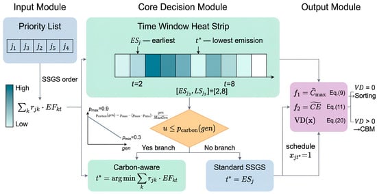
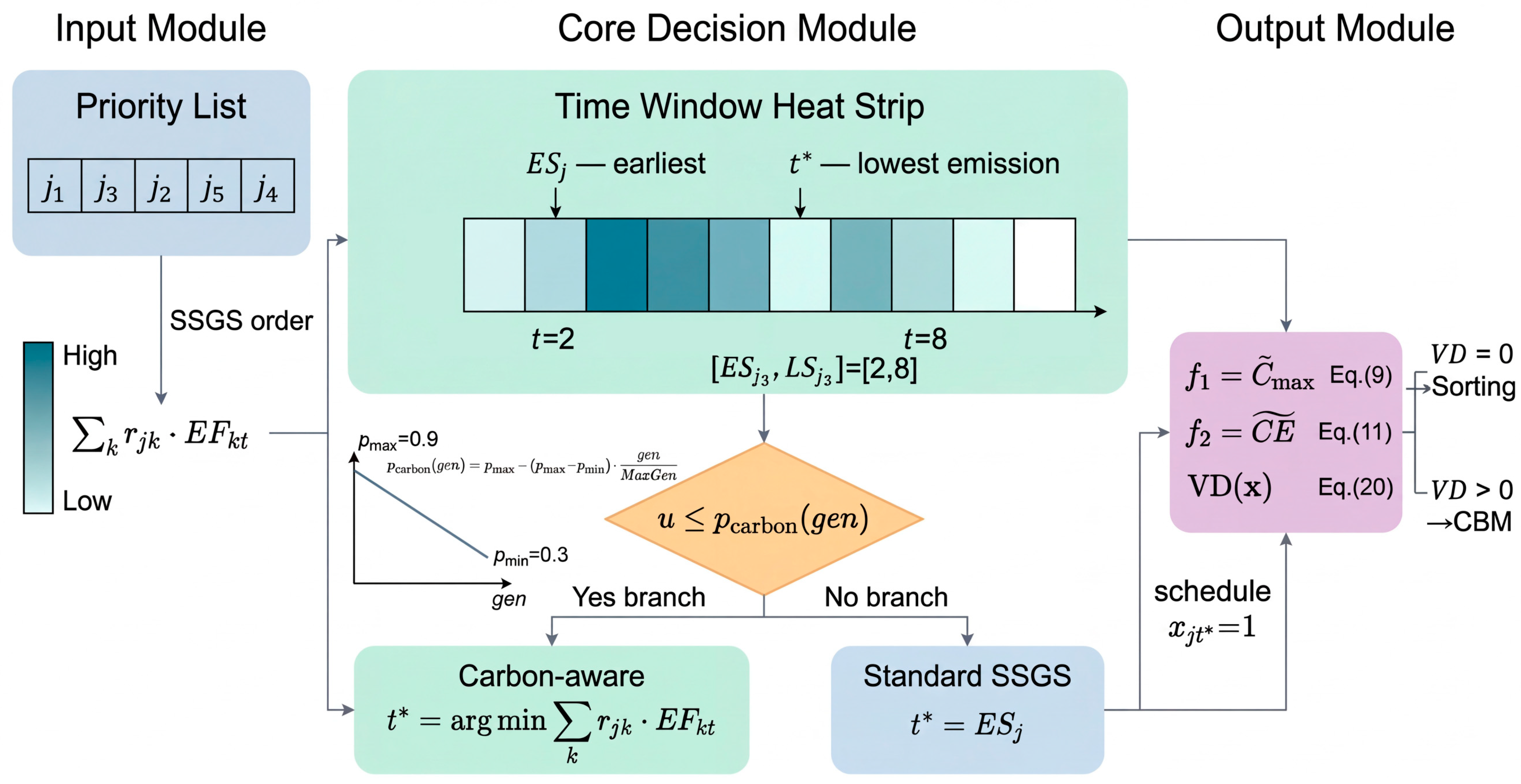
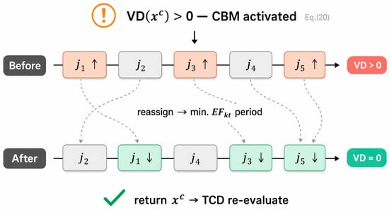
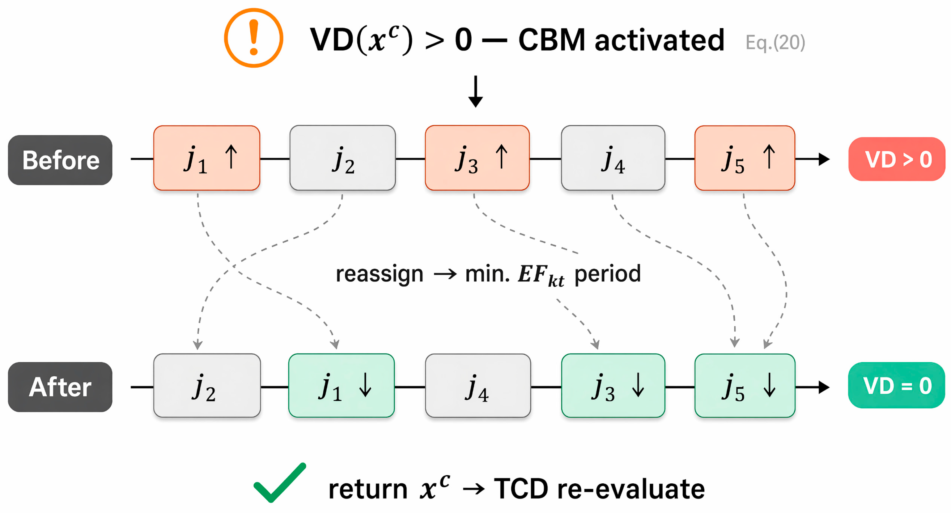
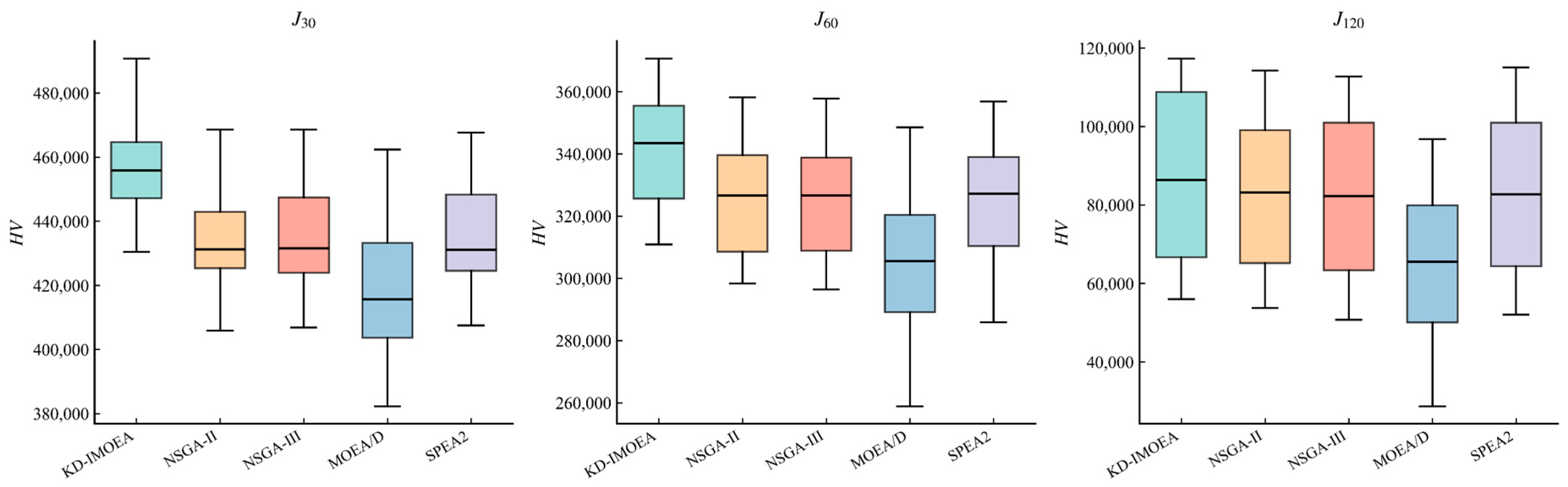
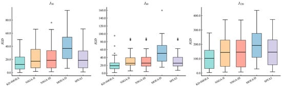
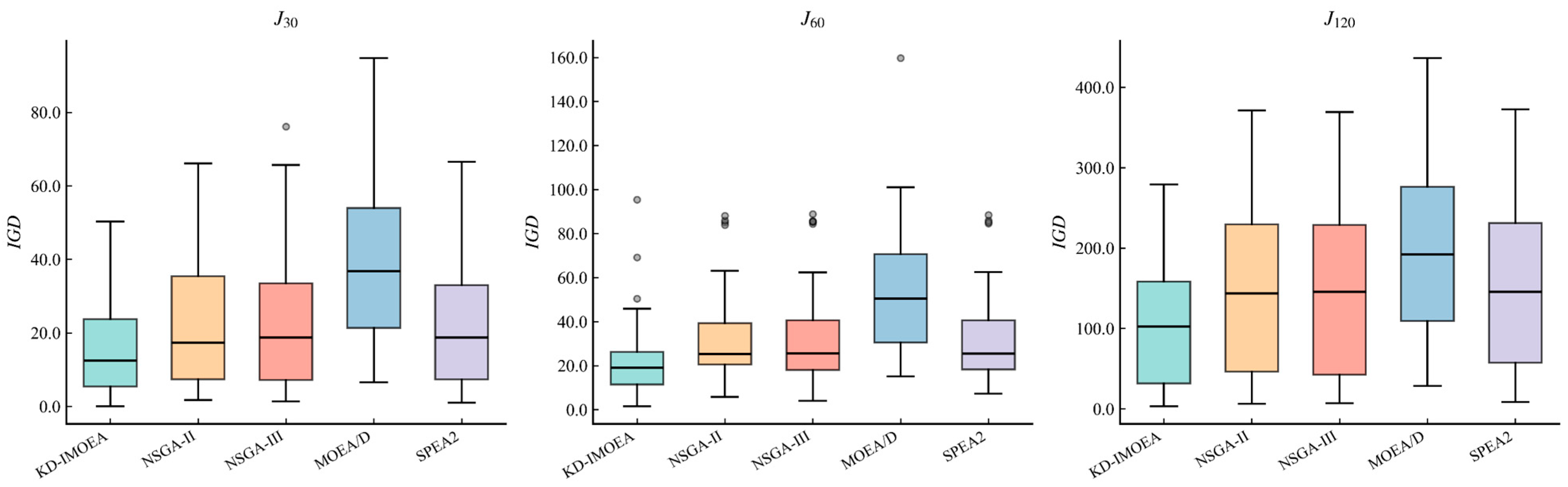
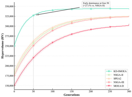
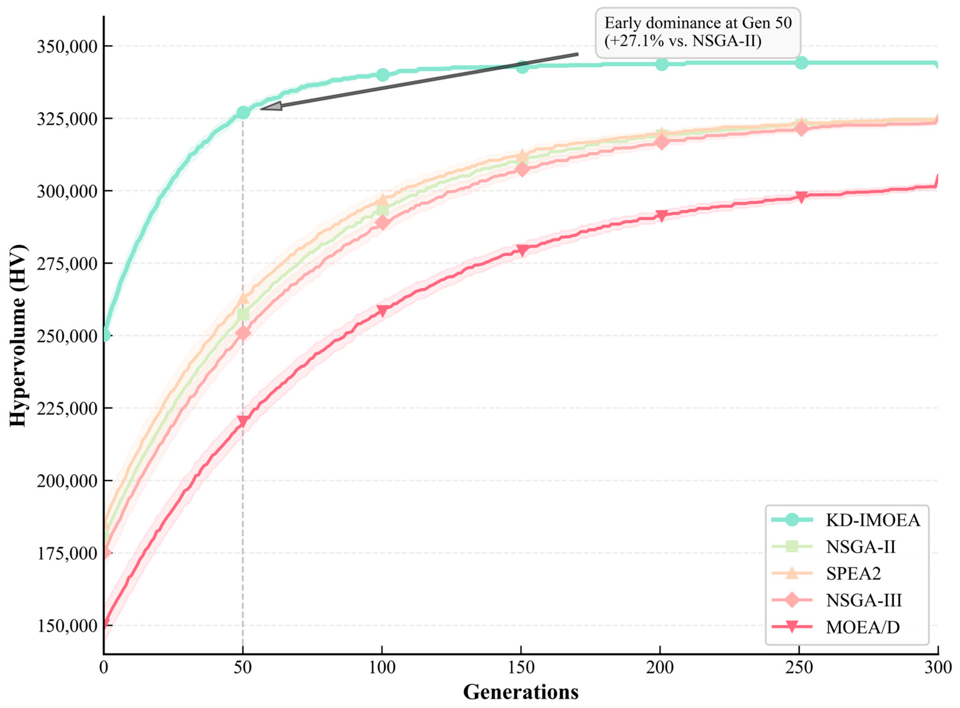
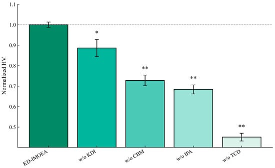
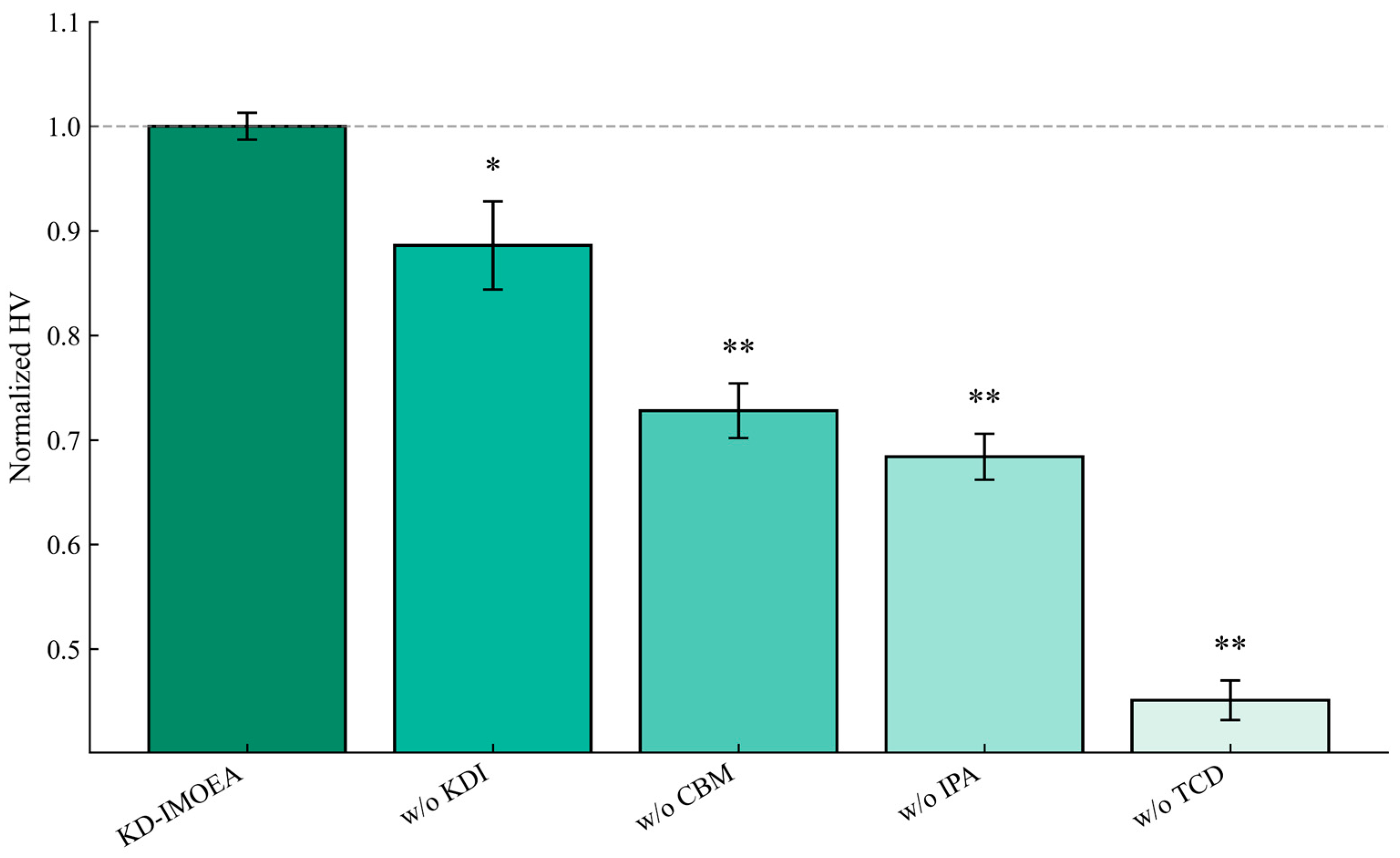
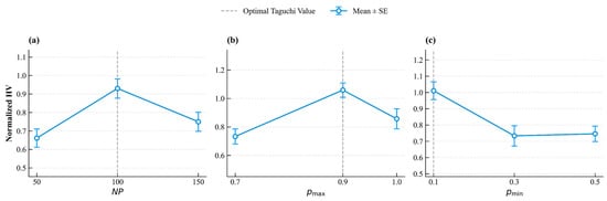
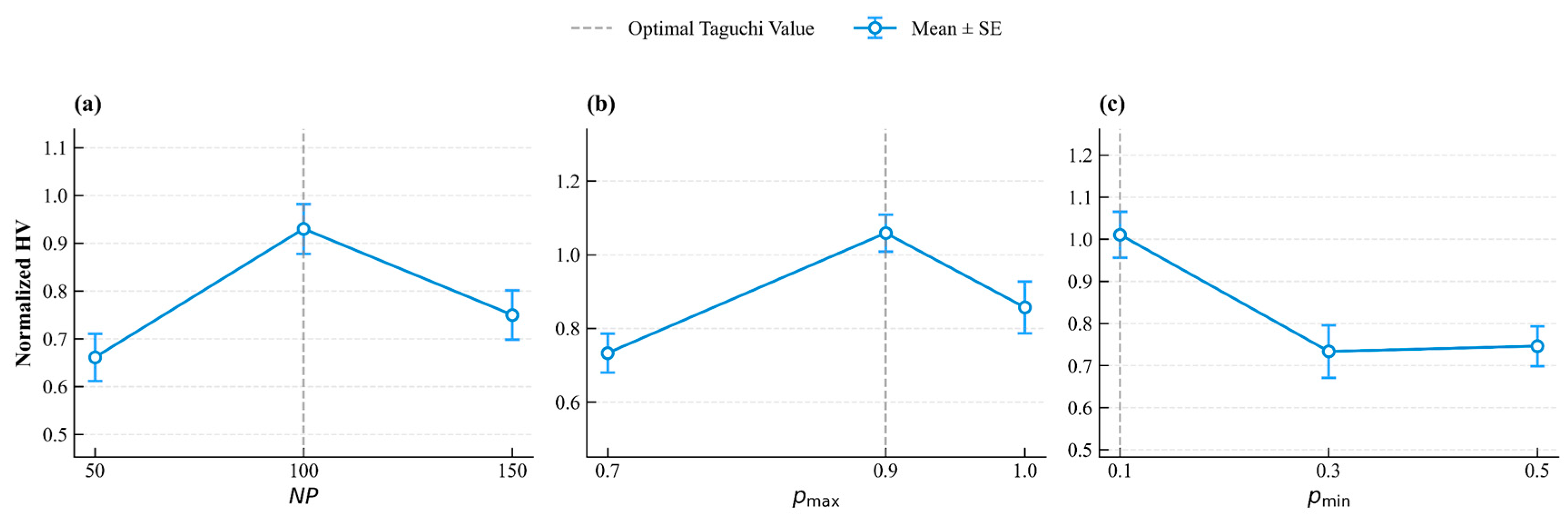


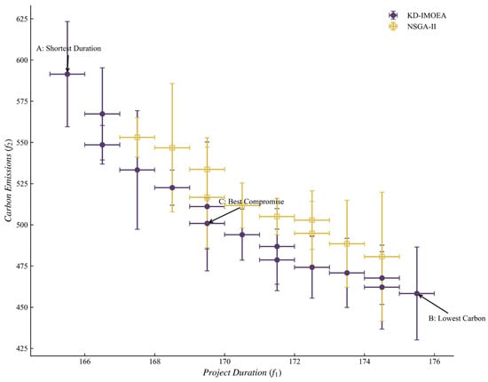
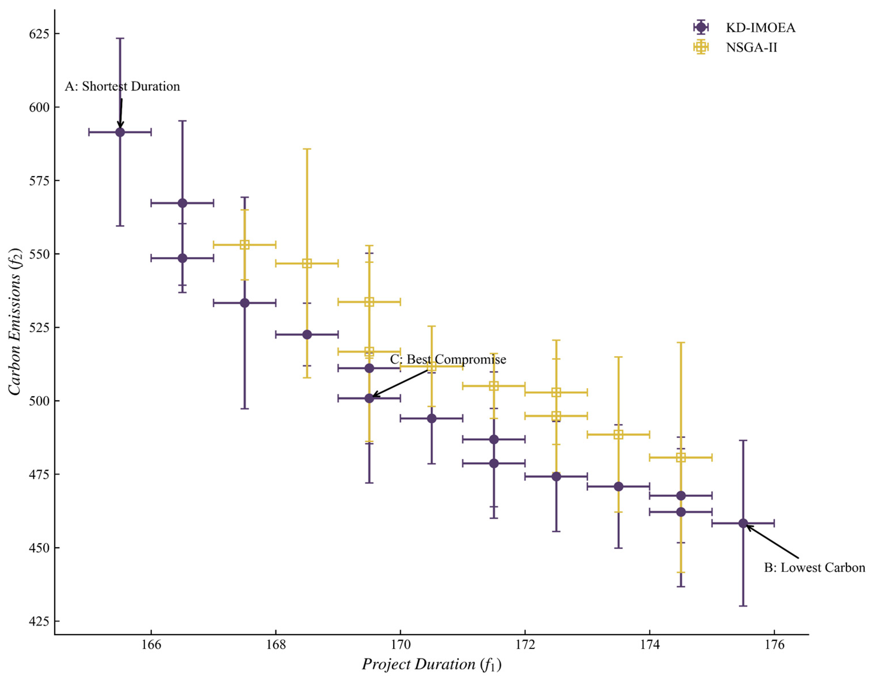
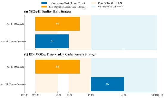
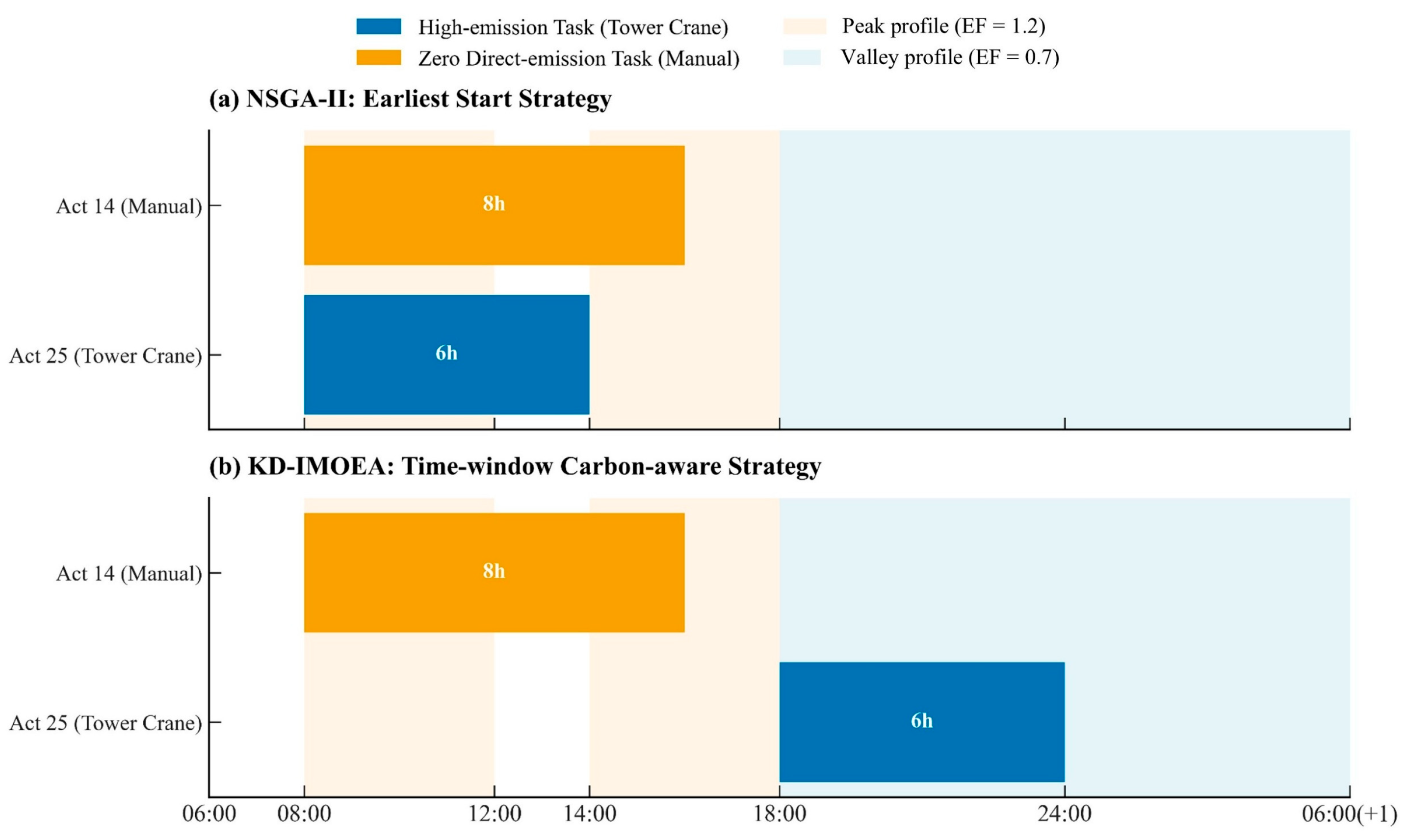

Disclaimer/Publisher’s Note: The statements, opinions and data contained in all publications are solely those of the individual author(s) and contributor(s) and not of MDPI and/or the editor(s). MDPI and/or the editor(s) disclaim responsibility for any injury to people or property resulting from any ideas, methods, instructions or products referred to in the content. |
© 2026 by the authors. Licensee MDPI, Basel, Switzerland. This article is an open access article distributed under the terms and conditions of the Creative Commons Attribution (CC BY) license.