


Abstract
Construction price indices play a critical role in shaping construction activity and determining the economic success of building projects in Germany, where they can serve as central inputs to cost planning and to updating trade-level project budgets over the planning and construction horizon. This paper develops a forecasting framework for 35 sub-construction price indices for office buildings, providing granular inputs for cost escalation and risk assessment. We employ regularized vector autoregressive models with exogenous variables (VARX) implemented via the BigVAR package and estimate them in a model-vintage design for an unbalanced panel. These high-dimensional models are benchmarked against compact VARX and vector error-correction models (VECM) that jointly forecast each target index with a small macroeconomic block consisting of the gross domestic product (GDP) and the three-month interbank rate. Candidate specifications are evaluated using mean absolute percentage error (MAPE) and out-of-sample root mean square error (RMSE), and the final forecasting model for each index is selected based on ex post MAPE. The results show that regularized VARX models capture dynamic interdependencies among the sub-indices and, for most series, outperform the VARX and VECM benchmarks. The resulting forecasts provide practitioners with trade-specific escalation factors that can support budgeting, contract design, and the mitigation of cost risk in office-building projects.
1. Introduction
In recent years, construction costs in Germany have exhibited pronounced volatility, which may have been influenced by external factors such as the COVID-19 pandemic and the war in Ukraine. These cost fluctuations have contributed to a slowdown in office and administrative building initiations measured in numbers of permits (Figure 1), as developers and contractors face greater uncertainty in budgeting and scheduling.
Figure 1.
Number of building permits for office and administrative buildings in Germany between 1991 and 2024. Data sourced from the German Federal Statistical Office [1].
Empirical evidence suggests also a measurable decline in construction output [2]. Concurrently, as Figure 2 shows, insolvency rates in the construction industry have risen, reflecting increased financial stress among market participants.
Figure 2.
Number of insolvencies in the construction industry in Germany between 2015 and 2023. Data sourced from the German Federal Statistical Office [3].
From a construction-economics point of view, the cost of an office building is not a fixed value during the planning and construction phase but rather highly sensitive to the timing of the project execution [4,5,6]. Since construction projects often span several years from initial concept to completion, the time dimension can become a central factor of cost escalation: Market developments and inflation manifesting themselves over time are reflected in costs via price movements. Internal operational problems that cause project schedule changes can amplify these influences [7]. Cost escalations driven by construction price increases and long project durations can account for a substantial share of construction costs in building projects [7,8].
In German practice cost planning follows different service phases defined in the national standard for construction costs DIN 276. At early stages, cost frameworks and preliminary estimates are derived from approximate quantities and reference unit rates, which are then iteratively refined and updated as design, approvals, and procurement progress [4,5,9]. Cost determinations must always be linked to a clearly specified price base and reference date to control and monitor cost changes ([4], Ch. 4, 4.5.2). In the cost plan, DIN 276 initially organises costs in an element- or component-oriented structure. For procurement and cost control during execution, these costs are subsequently transformed into an execution- or trade-oriented structure that aligns with the work sections specified in part C of the German construction contract procedures (Vergabe- und Vertragsordnung für Bauleistungen Teil C, abbr. VOB/C). This transformation from an element-oriented to a trade-oriented cost breakdown, which is an integral part of cost determination and cost control [4,5], ensures that each cost item can be uniquely assigned to a specific work section. These work sections correspond closely to the sub-indices of the official German construction price statistics, which are likewise reported by trade. This correspondence enables a direct linkage between project-level cost components and the relevant construction price indices.
Let index the VOB/C work sections relevant for an office building and let denote the estimated cost of work section b at the base date . Each is obtained by summing the cost components assigned to this work section, where each component is defined, in line with the DIN 276 notions of reference unit and cost coefficient, as the product of a reference-unit quantity and a base-date unit price representing the cost coefficient. Denoting by the set of cost components in work section b, and by and the quantity and unit price of component , we have
The total project cost at the base date can then be written as
If denotes the value of the construction price index associated with work section b at the base date and its forecast at a future date , a simple and widely used approach is to adjust the base-date cost of each work section in proportion to the forecast index movement. The corresponding forecast of total project cost at horizon is
Equation (3) formalises how disaggregated construction price indices at the level of VOB/C work sections can be used to update an office-building cost plan from its base date to the expected price level at the time of tendering or completion. This explicit linkage between trade-level indices and project costs provides the economic motivation for the forecasting framework developed in this paper.
To address cost planning risks and improve cost control in the office building sector, this paper makes several contributions that directly respond to gaps in the existing literature. First, it departs from prior work, which typically models a single aggregate construction cost index in univariate or small multivariate settings for cost management purposes (e.g., [10,11,12,13,14,15]), by jointly analysing and forecasting a panel of 35 trade-level sub-indices for office buildings. This multivariate, trade-oriented design exploits cross-trade interdependencies and yields trade-specific development factors that can be used for more detailed and precise project-level cost planning and risk management than is possible with a single aggregate index. Second, to our knowledge, no previous construction-cost forecasting study has systematically addressed large, unbalanced panels of trade-level indices with staggered start dates. In practice, however, such unbalanced datasets are the rule rather than the exception. We therefore develop a model-vintage design that explicitly exploits staggered series start dates and uses all available data at each vintage to improve forecast performance under these realistic data conditions. Third, while existing forecasting studies generally treat construction price indices as stand-alone time series for high-level cost monitoring or budgeting (e.g., [10,11,15]), they rarely connect the forecasts explicitly to national cost-planning standards and workflows. We close this gap by linking the predicted indices directly to the German cost planning system, where trade-level indices can be mapped to VOB/C work sections and used to update cost plans. Fourth, by leveraging regularized VARX-L models introduced by Nicholson et al. [16] and implemented in the BigVAR package (Version 1.1.4) for R, the study shows that high-dimensional regularised VARX specifications can, over the period considered, outperform conventional small VARX and VEC models when forecasting a large, unbalanced panel. Finally, it combines the forecasting framework with a simple, data-driven price-dynamics indicator to contrast dynamic and non-dynamic price environments. The modular framework can be readily updated and applied to future forecasting tasks, offering practitioners and policymakers a robust tool for anticipating price trends and mitigating risk in a volatile market environment. Forecast accuracy is further assessed by benchmarking the high-dimensional BigVAR forecasts against compact VARX and VEC models with real macroeconomic covariates, using MAPE and RMSE as evaluation criteria.
2. Literature Research
The importance of this topic is underscored by a growing academic literature. A systematic search in the Scopus database (see search string in Appendix A.1) identified 30 relevant studies on forecasting construction price indices in the building sector since 2005. Numerous additional contributions address related questions in the civil-engineering and infrastructure context.
In what follows, we provide a concise overview of the identified studies. For clarity, we organize the corpus by primary methodological emphasis into: Univariate (Section 2.1) and multivariate (Section 2.2) time-series analyses, machine-learning approaches (Section 2.3), network-based methods (Section 2.4), and hybrid models (Section 2.5). Studies that primarily compare methods or do not fit neatly into a single category—particularly those benchmarking alternative models—are grouped under comparative studies (Section 2.6). Before summarising the literature and positioning the present work (Section 2.8), we review a set of studies on office-building costs (Section 2.7) to provide the wider context of the paper.
2.1. Univariate Time-Series Analyses
Ashuri and Lu [11] compare the applicability and predictive performance of univariate time-series models for construction cost indices (CCIs) and find that a seasonal autoregressive integrated moving average (SARIMA) model provides the highest in-sample forecasting accuracy, while Holt–Winters exponential smoothing is the most accurate model for out-of-sample forecasts. Moon and Shin [17] build a univariate interrupted ARIMA for Engineering News-Record (ENR) CCI that embeds the June 2008 recession as an intervention and consistently beats ARIMA and Holt–Winters on a 12-month holdout. Moon, Chi, and Kim [12] confirm long memory in ENR CCI via rescaled range analysis and show that the developed autoregressive fractionally integrated moving average (ARFIMA) model delivers on average 9.5% lower average mean absolute percentage error than ARIMA. Zhao, Mbachu, and Zhang [18] show on New Zealand residential building cost indices that Holt–Winters exponential smoothing is more accurate for one- and two-story houses, while seasonal ARIMA is superior for townhouses, apartments and retirement villages, concluding that both are reliable depending on data characteristics.
2.2. Multivariate Time-Series Analyses
Shahandashti and Ashuri [13] identify vector error correction (VEC) models as appropriate for forecasting ENR’s CCI and show that bivariate VEC models (CCI and producer price index (PPI), CCI and crude oil price) outperform univariate approaches such as seasonal ARIMA and Holt–Winters exponential smoothing in out-of-sample predictions. Xu and Moon [14] develop a bivariate cointegrated vector autoregression (VAR) (CCI and CPI) and show on 2006–2010 out-of-sample tests that it delivers significantly lower errors than Holt–Winters benchmarks, while also offering stochastic (Monte Carlo) forecasts for uncertainty and risk assessment. Moon and Shin [19] develop a VEC model-based CCI forecasting method using Google search query frequencies, select “project manager salary” as the final driver from 396 candidates via cointegration and diagnostics, and show it outperforms a CPI-based cointegrated VAR benchmark. Choi, Ryu, and Shahandashti [20] examine city-level CCIs for 20 U.S. cities and evaluate four linear forecasting approaches, including ARIMA and VEC models augmented with macroeconomic indicators. They find no universally best model—the top performer depends on the city. Their guidance: Use multivariate models when local leading indicators are available; otherwise, opt for a parsimonious ARIMA.
2.3. Machine Learning
The first machine learning approach in the identified works was applied by Wang and Ashuri [21]. The authors apply two algorithms—k-nearest neighbors (k-NN) and perfect random tree ensembles (PERT)—to forecast the ENR CCI. Both methods improve forecast accuracy over benchmark time-series models (ARIMA, seasonal ARIMA, and VAR with CCI and CPI/PPI) across short-, mid-, and long-term horizons. Dong, Chen, and Guan [22] use a long short-term memory (LSTM) neural network to forecast a CCI, leveraging 16 economic, energy and market indicators to capture timeliness and long-range dependence. Compared with a support vector machine (SVM) baseline, the LSTM achieves higher short-term accuracy with less tuning; results hinge on careful feature selection but are limited by sparse data and a short-horizon focus. In the last machine learning paper examined Al Kailani et al. [23] evaluate k-NN, random forest and XGBoost algorithms for forecasting Jordan’s CCI, benchmarking them against linear regression and ARIMA. All three machine learning models outperform the traditional baselines; random forest attains the best accuracy, with the lowest MAPE and RMSE. Alzara et al. [24] develop a macroeconomic-aware deep-learning framework for forecasting a localized CCI in Egypt. Using LSTM and gated recurrent unit (GRU) models and a set of macroeconomic, monetary, foreign-exchange and energy indicators, they obtain very high out-of-sample forecast accuracy, with GRU slightly outperforming LSTM on several error metrics. The authors also demonstrate how the resulting CCI forecasts can be translated into project-level civil-works cost projections.
2.4. Network-Based Approaches
We now move on to the recently widespread network-based approaches: Zhang, Ashuri, and Deng [25] propose a two-stage forecasting model that first converts a time series into a visibility graph and uses link prediction to produce preliminary forecasts; these are then adjusted by a rule-based fuzzy-logic system. Using both in-sample and out-of-sample tests on CCI, TAIEX and student-enrollment series, the model attains high predictive accuracy; for the CCI case, it outperforms benchmark methods (Holt exponential smoothing, Holt–Winters, ARIMA, seasonal ARIMA). Zhang et al. [26] also present a network-based approach in which time series are first converted into a visibility graph and future values are predicted via link prediction. In one-step-ahead forecasts, the proposed model achieves lower MAPE than simple moving average (SMA) and SARIMA but higher mean squared error (MSE) and mean absolute error (MAE). In multi-step forecasts, the method outperforms SARIMA in terms of MAPE; for longer-horizon forecasts its accuracy is mid-pack compared with other approaches. Mao and Xiao [27] transform ENR CCI into a visibility graph, use link-prediction to derive node similarity, generate two forecasts (adjacent and linear-approximation) and combine them with distance weights, achieving slightly lower MAPE than SMA and Zhang et al.’s network baseline. Hu and Xiao [28] propose a reconstructing-forecasting method: A series is reconstructed, mapped to a directed visibility graph, and an improved random walk yields node-similarity–based probability distributions for the next value. On CCI (and other series), it outperforms ARIMA, SARIMA and a prior visibility-graph baseline and shows robustness to observational noise. In their second work in 2022 Hu and Xiao [29] propose an efficient time-series forecaster that converts a series into a visibility graph and computes node similarity via a new multi-subgraph similarity measure. The normalized similarity distribution is then used to predict the next value. The method was tested with CCI and financial data and compared to ARIMA, SARIMA and Holt-Winters benchmarks. The presented method consistently achieved the highest prediction accuracy. Hu and Xiao [30] introduce a network self-attention approach for forecasting, in which a time series is mapped to a visibility graph, node features are derived via random walks and a Recurrent NN learns similarity scores that are Softmax-normalized to weight the next-step prediction. On CCI data the method achieves the lowest error vs. ARIMA, SARIMA and a prior visibility-graph baseline from Zhang et al. [25]. In the subsequent year Hu and Xiao [31] introduce prediction based on fuzzy similarity distribution (PFSD), a time-series forecaster built on the fuzzy cognitive visibility graph: The series is mapped to a directed, weighted graph, node similarity is computed via a new weighted multi-subgraph similarity metric and a fuzzy similarity distribution is used for prediction. In benchmarks against ARIMA, exponential smoothing and feedforward NNs, PFSD attains state-of-the-art accuracy on annual and quarterly datasets, but its performance deteriorates at long horizons due to diminishing memory effects. A novel forecasting method that converts time series into visibility graphs and computes node similarity via a superposed random walk is proposed by Zhan and Xiao [32]. Unlike prior approaches, it forms predictions by weighted averaging over multiple similar nodes rather than using only the single closest match. Tested on CCIs among other series, the method attains the lowest forecast errors across all examined cases.
2.5. Hybrid Approaches
Combined—so-called hybrid—approaches in the field are presented now: Cao et al. [33] propose a new approach—the self-adaptive structural radial basis neural network intelligence machine to forecast Taiwan’s CCI. In a first step, multivariate adaptive regression splines analyze the importance of different factors for the CCI; the factors identified as significant are then fed into a radial basis function NN for prediction. The model outperforms competing artificial intelligence (AI)/statistical baselines as well as ARIMA models. Xie and Fang [34] developed a hybrid forecasting model for a CCI that combines a grey model with a backpropagation neural network. The hybrid model’s accuracy is compared with the respective single models. For one of the two forecasted quarterly values the hybrid model shows a slight reduction in error, for the other quarter it does not improve over the single approaches. Zhao et al. [15] employ a transfer-function modeling framework—integrating time-series analysis, regression and cross-correlation—to forecast the building cost index in New Zealand. Compared with an univariate ARIMA benchmark, the proposed model attains lower prediction errors, as measured by MAPE and RMSE. Kim et al. [35] propose a hybrid ARIMA–Artificial NN (ANN) model for city-level CCI and, versus standalone ARIMA and ANN, report higher accuracy across short-, medium-, and long-term horizons at both national and city scales. Improvements in precision are attributed to ARIMA’s linear and ANN’s nonlinear modeling strengths. Myrvang and Liu [36] compare a hybrid ARIMA-ANN, ARIMA and ANN for forecasting construction cost indices over medium- (5-year) and long-term (10-year) horizons. The hybrid model performs best at the medium horizon, while the ANN yields the most accurate long-term forecasts.
2.6. Comparative Studies
Finally, works are presented that primarily represent comparative studies. Hwang [37] contrasts classical linear regression with dynamic regression and shows that the latter yields superior ex post, out-of-sample forecasting performance. Hwang [38] develops an univariate autoregressive moving average (ARMA)(5,5) and a multivariate VAR(12) model (with CPI) for forecasting the ENR CCI, finds ARMA(5,5) slightly more accurate than VAR(12), shows both beat simple industry averaging methods and notes that dynamic regression models marginally outperform the new time-series models in his comparisons. Elfahham [39] compares in his work the forecasting accuracy of neural networks, linear regression, and univariate autoregressive time-series analysis using the Egyptian construction cost index, which he also derives, and finds that the most accurate results are achieved with univariate autoregressive time-series models. Aslam et al. [40] conducted a similar study: The authors derive a materials-based construction cost index for Pakistan and use the different forecasting models NN, linear regression and autoregressive model for CCI predictions. Evaluated by mean error, RMSE, MAE, and Theil’s U, the neural network achieves the highest accuracy while the regression and autoregressive model perform similarly with only slightly larger errors. Aydinli [41] evaluates with Holt–Winters, ARIMA, long-short term memory (LSTM), and gated recurrent units four models on monthly CCIs for nine European countries under two scenarios (S1: stable; S2: fluctuating) and three horizons (12/24/36 months). In the short term, models distinguish S1 from S2, but S1 leaders rarely lead in S2 and few differences are statistically significant—suggesting limited short-term impact of shocks on costs and forecast accuracy—whereas in the medium and long term S1–S2 gaps become significant, with machine learning (especially LSTM) often outperforming Holt–Winters/ARIMA, though no single model dominates across countries.
2.7. Office-Building Construction Cost Studies
Empirical research on office real estate has demonstrated the economic importance of this sector and analysed it from multiple perspectives, including portfolio performance, interest-rate sensitivity, and diversification benefits [42,43,44]. Since the present study is ultimately concerned with projecting future costs of office buildings, it is also closely related to work that models office-building construction costs at the project level. Early parametric approaches derive closed-form cost equations from cross-sectional data. Using historical parameter costs from Engineering News Record, Karshenas [45] develops a predesign cost-estimating method for multistorey steel-framed office buildings, expressing total cost as a power function of typical floor area and building height and showing substantially reduced variability compared with simple square-foot cost-book methods. Li, Shen, and Love [46] propose stepwise multiple regression models for reinforced-concrete and steel office buildings in Hong Kong, based on historical project data that are first normalised by a construction price index. Their models predict realised project costs with percentage errors typically within a few points. More recent studies extend these parametric approaches. Alshamrani [47] develops an initial-cost forecasting model for mid-rise green office buildings, using multiple linear regression on RSMeans-based datasets to relate cost per square foot to structural system, envelope type, and key geometric parameters, with all costs standardised via city cost indices. Chen et al. [48] develop machine-learning cost estimation models for office buildings at the decision-making stage, comparing back-propagation NNs and SVMs on 110 completed projects with dimensionality reduction via principle component analysis (PCA) and grey relational analysis. Across repeated train–test splits a PCA-based SVM with grid-search optimisation delivers the best performance, offering a practical tool for early-stage office cost prediction. Complementary to these estimation models, Starczyk-Kołbyk and Jędras [49] analyse a high-rise office building in Warsaw using an integrated risk-matrix and Monte-Carlo framework, identifying twelve key threats and opportunities and showing that an unusual increase in the costs of factors of production is among the most influential cost risks.
Taken together, these office cost studies demonstrate that regression-based, machine-learning and simulation-supported models can provide reasonably accurate early-stage project cost estimates and risk assessments when supplied with suitable design and cost-index information. In contrast, the present paper does not propose a new project-level cost formula. Instead, it develops a time-series framework for forecasting official trade-level construction price indices that feed into established German cost-planning procedures, thereby providing dynamic input factors that can be combined with existing project-level models and risk analyses to assess future office-building costs.
2.8. Literature Summary and Positioning of the Present Study
Summarizing, the literature has not identified an universally superior method for forecasting construction price indices. Predictive accuracy depends, among other factors, on data availability, horizon length and the stochastic properties of the series. Univariate approaches such as ARIMA and exponential smoothing remain competitive benchmarks, especially when only a single index is of interest and no reliable leading indicators are available. Where suitable drivers can be identified, multivariate time-series models—particularly VAR and VECM specifications—tend to improve forecast performance by exploiting cointegration and leading–lagging relationships between construction cost indices and macroeconomic variables or sector-specific indicators (e.g., [13,14,19,20]). Machine-learning, network-based, and hybrid models further expand the toolbox and can yield gains in specific settings, but they are typically applied to individual indices or small systems rather than to large panels of construction price series.
Distinct from most prior work, which focuses on single indices or low-dimensional bivariate systems, the present study jointly models a large panel of 35 interrelated office-building price indices. From an economic and statistical perspective, these indices form a coupled system: Common shocks to wages, materials, and demand propagate across trades, and some trades respond earlier than others. Vector autoregressive models with exogenous variables (VARX) provide a natural framework to capture such cross-series dynamics while simultaneously incorporating macroeconomic conditions and seasonal effects. Regularized VARX models (VARX-L) are particularly well suited to this task. First, they can exploit cross-series feedback and common factors, making systematic use of the information contained in the panel rather than treating each index in isolation. Second, the exogenous component accommodates seasonal dummies and scenario variables such as a price-dynamics indicator, enabling realistic responses to economy-wide shocks and the construction of economically meaningful scenarios. Third, shrinkage controls parameter proliferation in short and unbalanced samples, stabilizing estimation when the number of series and lags is large relative to the effective sample size. In parallel to these high-dimensional specifications, we also consider compact VARX and VECM models in which each target index is modelled together with a small macroeconomic block as reference models.
Importantly, the study does not propose an innovative cost determination method at the project level. Instead, it builds on established German cost planning practice and the transformation from element- to trade-oriented cost structures, and develops a time-series–based escalation approach: Forecasts of official trade-level construction price indices are used to update office-building cost plans from a documented base date to future points in time. In this way, the contribution of the paper lies in linking advanced multivariate forecasting methods to existing cost planning frameworks, jointly addressing a panel of 35 trade-level indices, demonstrating that regularized high-dimensional VARX models can outperform conventional small VARX and VEC specifications in this setting, and introducing a model-vintage design, thereby providing a data-driven tool for anticipating future office-building costs rather than redefining how base costs are estimated.
From a risk-management perspective, the integrated risk assessment for a high-rise office building by Starczyk-Kołbyk and Jędras [49] highlights that an unusual increase in the costs of production factors is among the most critical threats in office projects, yet risk probabilities and impacts are typically elicited from benchmark investments and expert judgement. The present study is complementary in that it provides data-driven forecasts of disaggregated construction price indices for 35 office-building trades, offering a statistically grounded basis for quantifying exactly this type of cost-escalation risk and for replacing purely judgemental escalation assumptions in project-level risk assessments and Monte Carlo simulations.
3. Materials and Methods
3.1. Data Sources
The empirical analysis draws on the construction price indices for office buildings published by Germany’s Federal Statistical Office [50]. The indices are published in GENESIS table 61261-0002. The individual indices measure the temporal (quarterly) evolution of construction service prices and are rebased to 100 in a designated base year. Currently, prices for 183 “price representatives” (individual construction services) are surveyed quarterly by the state statistical offices from roughly 5000 construction firms. Raw observations are first aggregated to state indices (“State measurement figures”) and then to national indices (“National measurement figures”) using turnover-based weights. Finally, building-specific weighting schemes [51] combine the price representatives into indices at different levels of granularity, enabling reporting for both detailed trades and higher aggregates [52]. For the empirical analysis, all series are converted to real terms by deflating with the German CPI [53].
In total, the dataset comprises 36 subindices, though not all are available from the beginning of the sample. Table 1 summarizes the number of series starting at the different points in time and the observation count per series.
Table 1.
Summary of the survey periods and associated data points for the 36 time series of the construction price indices for office buildings. Q1 refers to the first quarter of the respective year.
As the table indicates, the most recently introduced series contains only 18 observations. If all 36 series were included in a specification with four lags and four exogenous variables, ordinary least squares (OLS) estimation would entail, per equation, regressors (; see model explanation in Section 3.2). Adding the observations lost to lagging and one degree of freedom implies a minimum of 158 observations per series. Because a data share of only is small even for regularized models, the most recent series is excluded from the analysis. Restricting attention to the remaining 35 series already yields of the sample size required for an OLS fit per equation, making a regularized approach substantially more tractable.
For one set of small-scale models, the VARX and VECM specifications are augmented with German macroeconomic indicators that capture the overall state of the economy and monetary conditions. Specifically, we include real gross domestic product (GDP) and an inflation-adjusted three-month interbank rate as endogenous variables alongside the target construction price index. GDP is widely recognised as a key driver of construction activity and construction cost indices. Empirical studies for the ENR Construction Cost Index and for housing and construction markets in various countries report a strong positive association between GDP and construction prices [54,55,56,57].
Short-term interest rates, in turn, summarise the stance of monetary policy and the cost of capital. Prior work identifies prime lending rates, central-bank policy rates and related short-term interest-rate measures as important determinants of building material prices, construction costs and real estate prices, and uses them as leading indicators in construction cost and highway cost models [54,55,56,58].
Recent macroeconomic-aware forecasting frameworks for construction costs likewise combine GDP and central-bank interest rates with other macro-financial indicators to predict construction cost indices [24]. In line with this literature, we work with real GDP and a real three-month interbank rate, so that the macro block captures real activity and real financing conditions rather than pure inflation. Quarterly GDP is obtained from Germany’s Federal Statistical Office [59], while the three-month interbank rates are sourced from the Federal Reserve Bank of St. Louis (FRED) [60]. Monthly series are aligned to the quarterly construction price data by sampling at the study’s quarterly timestamps.
3.2. Forecasting Method
3.2.1. VARX-Models
A VARX model with k endogenous and m exogenous time series, of lag orders , can be written as
where is the k-dimensional vector of endogenous variables at time t, is a coefficient matrix associated with the ℓ-th lag of . is a k-dimensional intercept vector and a k-dimensional innovation vector assumed to be white noise. The exogenous regressors are collected in , and denotes the corresponding coefficient matrix at exogenous lag j [16].
The coefficient matrices are obtained by minimizing the multivariate least-squares criterion given by
see [16]. Here, denotes the Frobenius norm, . The matrices and denote the combined engogenous and exogenous coefficient matrices respectively of all lags considered. It follows that a specification requires estimating parameters.
3.2.2. Vector Error Correction Models (VECM)
Many macroeconomic time series are non-stationary and integrated of order one, , but exhibit stable long-run equilibrium relationships. The framework of cointegrated vector autoregressions and their vector error correction representation provides a way to jointly model long-run equilibria and short-run dynamics [61,62].
Following Johansen [61] (Ch. 4) and Lütkepohl [62] (Ch. 6–8), a VAR(p) in levels for a k-dimensional vector can be written in vector error correction form as
where denotes first differences, are short-run coefficient matrices, collects deterministic or stationary exogenous variables (e.g., constants, trends, seasonal dummies), with associated coefficient matrix and is a zero-mean innovation vector, typically modelled as white noise. The matrix is the long-run impact matrix. If it has reduced rank , it can be factorized as , where the columns of the matrix define the cointegration relations and the matrix contains the corresponding adjustment coefficients.
Estimation of VECM parameters is typically based on the maximum-likelihood approach for cointegrated VAR models, taking into account the rank restriction for ([61,62], Ch. 7, Ch. 7). However, least squares and estimated generalized least squares estimators are also common choices ([62], Ch. 7).
3.2.3. Regularized VARX-Models
Because the number of parameters grows quadratically, VARX models quickly reach their limits when samples are low-frequency or otherwise short relative to the dimensionality of the system. To address this challenge, Nicholson, Matteson, and Bien [16] developed the VARX-L framework, which transfers Lasso-style regularization to vector time series and thereby substantially reduces the effective parameter space. An implementation is available in the open-source R package BigVAR (Version 1.1.4).
The core idea is to reduce the number of active coefficients via penalty terms. Accordingly, the general estimation problem in Equation (5) is augmented as follows:
The terms and denote penalty functions applied to the endogenous and exogenous coefficient blocks, respectively. The shared penalty parameter governs the strength of regularization and must be selected as part of model estimation. Specifically, Equation (7) accommodates different penalty functions. Table 2 summarizes the variants considered: Lag, Own/Other, Sparse Lag, Sparse Own/Other, Basic and Endogenous-First.
Table 2.
Regularization penalties for different model structures [16].
In the Lag specification, the entire coefficient matrix for each endogenous lag is treated as a single block, whereas for the exogenous variables each individual series forms its own group at each lag. The authors recommend this penalty when the series are similar—such as subindex series-making it a promising choice for the present application. The Own/Other model further partitions the endogenous coefficient matrices into diagonal (“own”) and off-diagonal (“other”) groups, aiming to capture settings with pronounced autocorrelation or cross-correlation. The Sparse Lag variant allows individual coefficients within an otherwise active lag block to be shrunk to zero. Sparse Own/Other extends this idea to the diagonal/off-diagonal partition. The Basic approach is computationally efficient and permits elementwise zeroing in both endogenous and exogenous coefficient matrices. Finally, the Endogenous-first penalty imposes a hierarchy in which exogenous predictors (and their coefficients) may enter at a given lag only if the corresponding endogenous predictors have been selected [16].
3.3. Study Procedure
We implement and investigate three configurations of multivariate time-series models that differ in scope and dimensionality. All specifications share the same set of deterministic and exogenous regressors: Three quarterly dummy variables (with the first quarter as reference) to capture seasonal effects and a binary price-dynamics indicator that flags periods of elevated price movements. The construction of this indicator is described at the end of this section.
In the low-dimensional specifications we first estimate conventional VARX systems (“mVARX”) in which each target index is modelled individually. For these models, the endogenous block consists of the target construction price index together with a compact set of macroeconomic variables. Cross-series lags from other construction indices are not included, which keeps these specifications computationally light and data-sparse. Given that several of the series and macroeconomic variables might be cointegrated, we additionally consider vector error-correction models with macroeconomic variables (“mVECM”). For each target index, we test for cointegration between the construction price index and the macroeconomic block and, whenever the Johansen tests indicate at least one cointegrating relationship, we estimate a corresponding small VEC model with the same set of macro variables as in the mVARX specification. These mVECM systems are likewise low-dimensional and computationally inexpensive. In the high-dimensional models (“BigVAR”), by contrast, all construction price indices are modelled jointly as the endogenous block, allowing dynamic spillovers and common shocks to propagate across the panel. Because the parameter space grows quickly with the number of series and lags, these systems are estimated with shrinkage/regularization using the VARX-L methods described above. We compare the ex post out-of-sample performance of all three configurations—mVARX, mVECM and BigVAR—and use the better-performing specification to generate ex ante forecasts of the construction price indices. To enable a subsequent comparison between phases of elevated and subdued price movements, we derive from the data a classification indicator that tags each period as either dynamic or non-dynamic with respect to price movements. The construction of this indicator is described next.
For the identification of historical periods with dynamic price developments (outliers), we compute the Z-value on the relative changes of the aggregate construction price index (see Section 3.1), where and denote the mean and standard deviation over the estimation window ([63], p. 6):
A period is classified as exhibiting high price dynamics if . This decision rule implies that the observed change deviates from the estimation-window mean by at least two standard deviations in absolute terms and aligns with employed outlier-detection rules in literature [64,65,66]. Assuming is approximately standard normally distributed, this tow-sigma cut-off implies that about of the observations fall into the non-extreme range, corresponding to a (two-sided) significance level of roughly . While alternative reasonable thresholds are conceivable and would primarily affect the number of flagged periods rather than the qualitative scenario logic, values below this threshold are treated as non-remarkable with respect to price movement. The resulting classification is shown in Figure 3, with dynamic periods marked by red dots. In total, 14 dynamic periods are identified.
Figure 3.
Illustration of identified periods with high price dynamics (red marker).
3.3.1. Conventional VARX-Models with Macroeconomic Variables (mVARX)
The first model group consists of conventional VARX systems. For each of the 35 target series, we estimate a small VARX in which the endogenous block comprises the target index together with two macroeconomic indicators—real gross domestic product (GDP) and the inflation adjusted three-month interbank rate in germany. Exogenous terms are restricted to three seasonal dummy variables (quarter-of-year indicators). Prior to estimation, all series are tested for stationarity using the augmented Dickey–Fuller (ADF) and Kwiatkowski-Phillips-Schmidt-Shin (KPSS) test. Series that appear non-stationary are differenced as required (see Table A1 and Table A2). In total, 35 VARX systems are estimated. The lag order is considered, and the final specification for each system is selected using the Akaike Information Criterion (AIC).To evaluate forecast accuracy using MAPE and RMSE, we generate ex post out-of-sample forecasts for the last 24 observations of each series.
3.3.2. Vector Error-Correction Models with Macroeconomic Variables (mVECM)
Within the second model group we again form a small system for each target index consisting of the construction price index and the same compact set of macro indicators as in the mVARX specification (GDP and the three-month interbank rate), and retain the quarterly dummies and the price-dynamics indicator as exogenous regressors.
To assess whether an error-correction representation is appropriate, we compute both the Johansen’s trace and maximum eigenvalue test statistics for the cointegration rank [67]. As discussed in Lütkepohl [68], the two statistics need not yield identical rank decisions. Following this guidance, we adopt the rank implied by the trace test as our primary criterion. Whenever the Johansen test (trace) indicates at least one cointegrating relationship, we estimate an mVECM with the corresponding rank. If no cointegration is detected, no VEC specification is estimated for that series. As Table A3 shows, cointegration can be established all of the 35 considered construction price indices, so a complete VECM-based forecast for all series is feasible.
For the cointegrated systems, the lag order of the underlying VAR in levels is selected by the Akaike Information Criterion from , consistent with the mVARX specification. The resulting VEC representation then contains lags of first differences and the estimated error-correction terms. These mVECM systems remain low-dimensional and computationally inexpensive. Their ex post out-of-sample forecast performance is evaluated in the same way as for the mVARX models, using MAPE and RMSE over the last 24 observations, and is compared to both the mVARX and BigVAR configurations.
3.3.3. Design of Regularized VARX-Models (BigVAR) Approach
As the third approach, we employ regularized VARX models (see Section 3.2.3) that jointly model and forecast a large set of construction price indices. As in the small-scale models in Section 3.3.1, the series are first transformed to stationarity, seasonal effects are captured by three quarterly dummy variables and the price-dynamics indicator enters as an additional binary exogenous regressor. We deliberately exclude macroeconomic variables from both the endogenous and exogenous blocks because the system is already high-dimensional and reliable ex ante forecasts for these covariates are unavailable over our evaluation window.
Table 1 documents that the constituent series begin at different dates. Because VARX models require a time-aligned sample, two competing strategies arise for our large models. One can (a) estimate on the longest horizon but restrict the cross-section to those indices observed throughout—maximizing the time dimension T while reducing the cross-sectional dimension N—or (b) retain the full set of indices and estimate only on the intersection period in which all series are available—maximizing N but shortening T. Intermediate compromises are also possible. To sidestep this trade-off and exploit the maximum information available for each index, we adopt an innovative model-vintage design: At every date on which additional indices become available, we estimate a separate VARX model on the longest contiguous window feasible at that vintage. This yields a sequence of models with expanding time spans and, when data permit, an enlarging cross-section. The procedure is illustrated in Figure 4.
Figure 4.
Schematic illustration of the model-vintage design (figure not to scale). Along the horizontal axis, the segments show the estimation windows for regularized VARX models 1–7, each starting when new series become available. The vertical extent of each segment reflects the number of construction price indices included in that vintage. For example, model 1 is estimated from 1968 onward and contains 25 series, while later vintages include more series over shorter time spans.
Building on this design, within each model vintage we estimate all six considered single-penalty specifications available in BigVAR—Lag, Own/Other, Sparse Lag, Sparse Own/Other, Basic, and Endogenous-First—across seven configuration settings, yielding models. Due to the high dimensionality only lag orders are considered. For each model, the regularization hyperparameter is selected via rolling cross-validation. We first define a grid of candidate penalty values. For every , the model is re-estimated at each forecast origin t on the validation window and h-step-ahead forecasts are generated. Selection is based on the mean squared forecast error (MSFE):
where the average is taken over all forecast origins . Here, denotes the last observation used for the initial estimation, marks the end of the validation window, h is the forecast horizon, and denotes the Frobenius norm applied to the vector of forecast errors across series [16]. Ex post out-of-sample forecasts of all models are evaluated.
3.3.4. Comparison of Prediction Accuracy of All Employed Models Types
Using all three modelling approaches, we generate ex post out-of-sample forecasts for the last 24 available observations of each construction price index and compare accuracy across model types. Reserving these 24 quarters for evaluation implies that the final observation used for parameter estimation is Q2 2019, so the models are estimated without direct influence from the subsequent COVID-19 pandemic and the war in Ukraine, while their forecasts are evaluated precisely over this turbulent period, in which the price-dynamics indicator enters as an exogenous dummy to help all specifications capture shifts in the price environment. For the high-dimensional BigVAR class, forecasts are obtained from the regularized specifications selected by the cross-validation procedure described in Section 3.2.3.
Forecast accuracy is evaluated by the mean absolute percentage error (MAPE),
and the root mean squared error (RMSE),
where H denotes the evaluation horizon (here ). MAPE is particularly suitable in our setting because errors are computed on level data whose values are well away from zero. Consequently, the measure does not suffer from the usual interpretational caveats ([69], Ch. 3.4). For each series, we use MAPE as the primary selection criterion, while RMSE is reported as a complementary measure of forecast accuracy and is only displayed for each series in Table A4, Table A5 and Table A6. For BigVAR, the model used for each series is the vintage–specification combination (year and penalty structure) that attains the lowest ex post out-of-sample MAPE for that series.
Figure 5 summarises the series-wise forecasting performance of the three model classes. At first glance, the MAPE levels across BigVAR, mVARX, and mVECM appear broadly similar for many indices, with only a few conspicuous outliers where one or both of the small-scale models performs noticeably worse. A closer inspection, however, reveals a clear ranking: BigVAR delivers the lowest ex post MAPE for 23 of the 35 series (and the lowest RMSE for 24 series), while mVARX attains the best MAPE in 10 cases (RMSE in 9 cases) and mVECM outperforms both competitors for only 2 series (RMSE in 3 cases). Thus, although the average error levels do not differ dramatically at first sight, BigVAR provides the most accurate forecasts for the majority of indices.
Figure 5.
Ex post out-of-sample forecast errors (MAPE) of all three model types (BigVAR, mVARX, mVEC) for each construction price index. Series are ordered by the MAPE achieved by the BigVAR specification. The numbers prefixed to the series names denote the Series IDs, which are used consistently in the subsequent figures.
The aggregated error measures in Figure 6 corroborate this ranking and highlight the overall superiority of the BigVAR models. On average across all series, BigVAR reduces MAPE and RMSE by about and index units, respectively, relative to the next-best model (mVARX). When the series are weighted by their contribution to the aggregate construction price index, the advantage increases to in MAPE and index units in RMSE. The global MAPE and RMSE, computed on the full forecast panel rather than series by series, also favour the BigVAR specifications, with gains of percentage points in MAPE and index units in RMSE. By construction, MAPE is invariant to whether it is computed series-wise and then averaged or directly from the full panel. In both cases, the same set of percentage-error terms enters the calculation with equal weight. Given the consistently superior forecast accuracy, we employ, for the ex ante out-of-sample projections, the best-performing BigVAR specification for each series.
Figure 6.
Ex post out-of-sample MAPE and RMSE of all three model types, aggregated across series. Mean errors are computed as the unweighted average of the series-specific errors, weighted errors use the official subindex weights in the aggregate construction price index. Global errors apply the respective loss function to the full forecast panel at once.
3.3.5. Prediction of Price Indices
Finally, using the best-performing BigVAR specifications for each series, we generate out-of-sample forecasts for all construction price indices over the one-year period immediately following the last available observation by iterating one-step-ahead predictions over the next four quarters. The scenario design is governed by the exogenous price-dynamics indicator: In scenario I (non-dynamic), the indicator is set to zero for the entire forecast horizon, whereas in scenario II (dynamic) it takes the value one in the first two quarters and zero thereafter. To quantify forecast uncertainty, we construct bootstrap-based prediction intervals. The near-term behavior of the indices under both scenarios is summarized in Section 4.
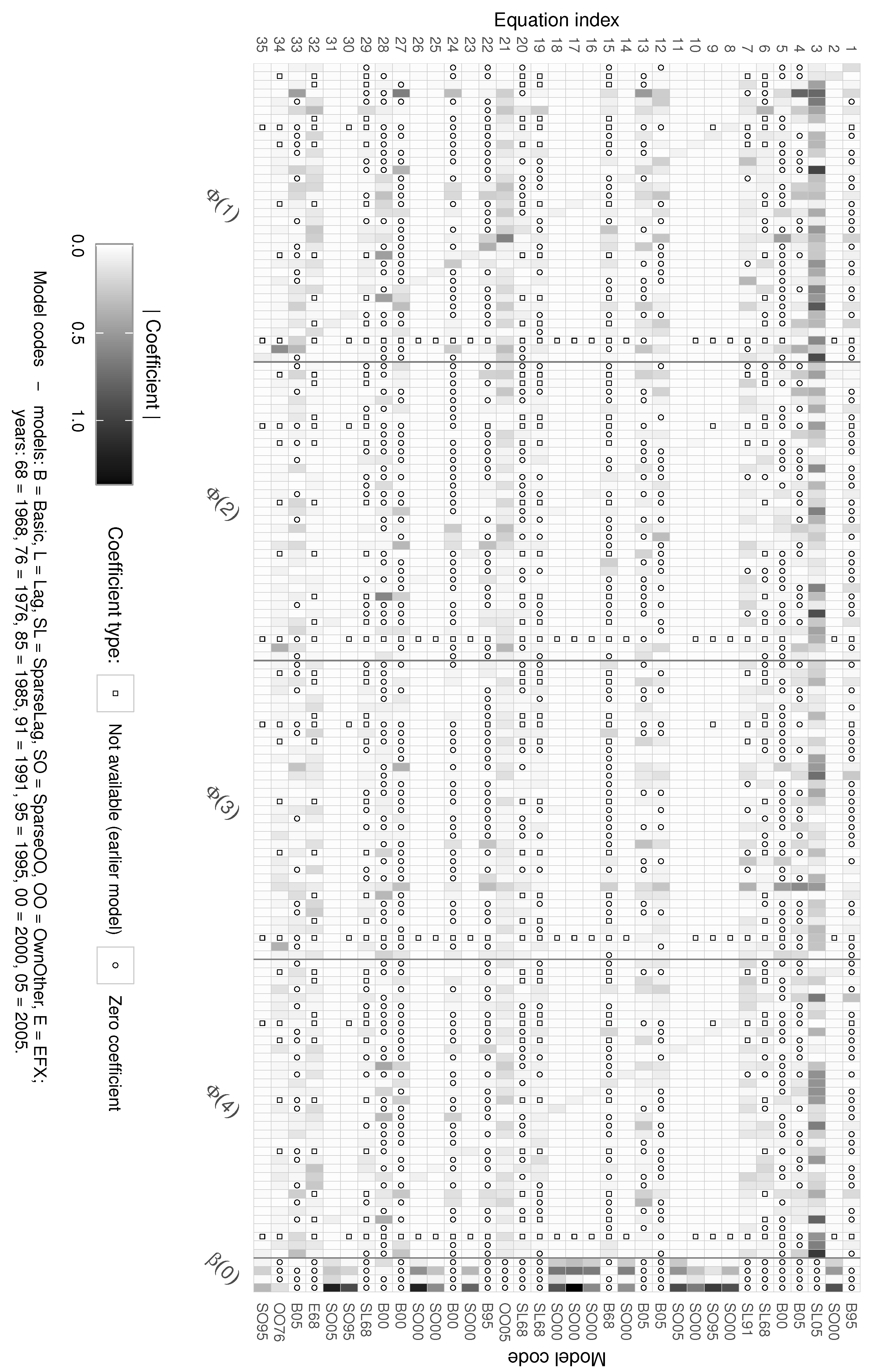
For illustration, Figure A1 displays the structure of the employed BigVAR system in terms of its endogenous () and exogenous () coefficient matrices. The primary y-axis indexes the equations, which correspond directly to the series IDs (e.g., those reported in Figure 5 or Table A7), while the secondary y-axis indicates the model vintage from which the coefficients are taken. For each equation, the plot thus shows the coefficient pattern of the specific model used to forecast that target series. Coefficients that are exactly zero, either due to the model-vintage design or as a result of regularization, are explicitly highlighted, and non-zero coefficients are shown with colour intensity proportional to their absolute value.
4. Results
Figure 7 compactly summarises the cross-sectional behaviour of the 35 construction price indices over the four forecast steps under scenarios I and II. For each forecast step, the solid line reports the cross-series mean of the percentage change relative to the last observed index value on 15 May 2025. The dashed and dotted lines trace the upper and lower envelopes of the cross-section, defined as the largest positive and largest negative percentage changes across all series, respectively. The shaded area between these two envelopes represents the corresponding range of forecasted changes at each horizon.
Figure 7.
Summary of BigVAR forecast results over the four forecast steps under scenario I (non-dynamic) and scenario II (dynamic). For each step, the solid line shows the cross-series mean of the percentage change relative to the last observed index value on 15 May 2025, the dashed and dotted lines show the upper and lower envelopes given by the largest positive and largest negative changes across the 35 indices, and the shaded area indicates the resulting range.
The envelopes for the two scenarios exhibit both similarities and marked differences. The lower envelope is identical in scenarios I and II and ranges from roughly in the first forecast step to about in the second step, before moving back to around at the end of the horizon. This reflects the fact that the same indices generate the largest negative real changes in both scenarios and that, for these particular trades, the scenario distinction via the price-dynamics indicator does not materially affect the forecast path. By contrast, the upper envelope diverges substantially: Under scenario I, the largest positive change increases in an almost linear fashion from approximately in the first step to around in the fourth step, whereas under scenario II it rises from roughly to nearly over the same period. The mean change follows the same pattern at a lower level, increasing from about to in scenario I and from about to in scenario II. Overall, the figure indicates that, while real construction prices are expected to increase on average in both scenarios over the forecast year, the dynamic-price environment in scenario II is associated with substantially stronger upside movements, as reflected in both the higher mean and the more rapidly widening upper envelope.
A detailed inspection of the series-level forecasts (see Table A7 and Table A8) confirms that only two indices exhibit slight real declines over the full forecast horizon relative to the last observed value: “carpentry and woodworks” (scenario (S) I: , scenario (S) II: ) and “concrete stoneworks” (S I: , S II: ). The detailed values also make clear that these two series do not differ across the scenarios, as their forecast paths are identical under scenario I and scenario II. These modest decreases may be interpreted as easing real prices in trades that are particularly exposed to cyclical demand or competitive pressure in the finishing market, for example because previously elevated margins are compressed when order books thin out, and, consistent with the identical forecasts under both scenarios, they appear relatively insensitive to the temporary shifts in aggregate price dynamics that underpin the scenario distinction. By contrast, the strongest relative increases are observed for “insulation and fire protection works on techn. systems” (S I: , S II: ). The next-largest real increases in scenario I occur for “electrical, security, and information technology systems” (S I: , S II: ) and “gas, water, and drainage systems within buildings” (S I: , S II: ) while in scenario II for “shoring works” (S I: , S II: ). All four trades are labour- and technology-intensive and strongly affected by regulatory and technical requirements (e.g., energy efficiency, fire safety, building services integration). In a German context, rising real costs in these areas are consistent with persistent skilled-labour shortages in technical building services, which can push up real wages, as well as continued pressure from material and equipment prices.
The projected paths with confidence intervals of the six sub-indices that carry the largest weights in the aggregation to the top-level index are shown in greater detail in Figure 8. These six series are “earthworks”, “concrete works”, “metal construction works”, “electrical, security, and information technology systems”, “heating and central water heating systems” and “drywall works”. For each series both scenarios are depicted. Both “concrete works” and “metal construction works” display almost flat real price paths, with only small fluctuations over time and very similar confidence bands across scenarios. The scenario design does not materially affect the projected development of these two trades. These projections are entirely data-driven and reflect historical patterns in the underlying time series, including past changes in demand, construction cycles, and the macroeconomic environment as captured in the observed index data. Within this purely empirical framework, a plausible interpretation is that these trades represent mature core activities with long-established technologies, standardised execution methods, and relatively competitive market structures. In the absence of strong additional demand impulses in the historical record, real prices in such stable segments can remain broadly constant, as productivity gains and incremental process improvements may offset a portion of the underlying cost pressures. These interpretations should be understood as deductive, economically motivated readings of the data patterns rather than the result of explicit macroeconomic modelling.
Figure 8.
Ex ante out-of-sample forecasts with confidence intervals for the six most heavily weighted sub-indices, shown under scenario I (non-dynamic) and scenario II (dynamic).
By contrast, the remaining four series all exhibit noticeable real price increases. In scenario I, the indices rise by roughly (“drywall works”) to (“electrical, security, and information technology systems”) index units over the forecast horizon. In scenario II, the corresponding increases range from about (“electrical, security, and information technology systems”) to (“earthworks”) units. Again, these forecasts are inferred solely from historical dynamics in the indices, which implicitly incorporate past macroeconomic conditions, sectoral demand shifts, and construction cycles. Within this data-driven setting, “electrical, security, and information technology systems” shows very similar trajectories in both scenarios and comparatively narrow confidence bands, which may be consistent with a robust underlying trend in real costs driven by the increasing complexity and penetration of building services (e.g., communication networks, security systems, and automation) and relatively stable demand. In contrast, “earthworks”, “heating and central water heating systems”, and “drywall works” all display a markedly stronger increase under scenario II. For “earthworks”, such a pattern may be associated with historical sensitivity to fuel and machinery costs and to fluctuations in infrastructure and foundation activity. For “heating and central water heating systems”, higher real prices align with observed tightening of energy-efficiency requirements and a gradual shift towards more sophisticated and capital-intensive systems. The pronounced rise in “drywall works” may reflect persistent pressures on skilled labour, evolving interior fit-out standards, and sustained demand in refurbishment and office reconfiguration, all of which can push real wages and material-intensive services upward when capacity is tight. The latter three indices also exhibit broadly similar confidence-interval widths, indicating comparable levels of forecast uncertainty across these key trades.
The extent to which the series’ trajectories differ or closely align between the two scenarios is examined in detail in Section 5. That section also discusses differences in the widths of the confidence intervals and analyzes the evolution of the aggregate index.
5. Discussion
The similarity of many forecasted series across scenario I (non-dynamic) and scenario II (dynamic) is evident from the difference D (scenario II − scenario I) shown in Figure 9. In the final forecast step, 15 series display substantial deviations (interpreted here as ). In all of these 15 cases scenario II yields higher real index levels than scenario I, while only the series “flooring works” and “thermal insulation composite systems” show slightly larger values in scenario I at the end of the forecasting horizon. In the first forecast step, 19 series have identical predicted values under both scenarios, by the final step, this number drops to 14, indicating that some trajectories diverge only gradually over time.
Figure 9.
Illustration of the absolute differences between the two scenario forecasts, computed as scenario II minus scenario I (S II − S I). The mapping from Series IDs to series names is shown in Figure 5.
The 19 coinciding series in the first step can be explained by the estimated coefficient structure in the global sparsity pattern shown in Figure A1. In particular, the fourth column of corresponds to the coefficient on the exogenous price-dynamics indicator. For 19 equations, this coefficient is shrunk to zero by the regularization procedure (highlighted in the plot), implying that the price-dynamics indicator has no direct effect on the one-step-ahead evolution of these series. As the forecast horizon increases, however, four of these series become indirectly affected via cross-series lagged values: The indicator influences other indices, and these, in turn, enter the equations for the previously unaffected series through lagged endogenous terms. These cross-lagged transmission channels are implied by the VARX structure of the individual vintage-specific models, but they are not directly visible in the aggregate sparsity pattern because each series is ultimately forecast from its own model, as indicated on the secondary y-axis in Figure A1. All of these mechanisms are purely data-driven: They result from the estimated dynamic relationships in the historical panel and from the regularization.
When the individual forecasts are aggregated to the composite CCI using the official weights, the resulting trajectories are shown in Figure 10. Both projected scenarios align well with the historical evolution of the index, with similarly increasing levels. As expected, the dynamic-price environment in scenario II leads to higher index values. The difference between scenarios widens monotonically over the forecast horizon but remains moderate in magnitude, amounting to about relative to the scenario I index level, or roughly index points, at the end of the forecasts. This gap should be interpreted as a model-based extrapolation of historical patterns in periods of elevated price movements, as encoded in the price-dynamics indicator and the estimated relationships. In economic terms, such developments can be associated with capacity constraints in materials supply, shortages of skilled labour, and temporarily strong demand, which are implicitly reflected in the historical data underlying the model.
Figure 10.
Representation of the aggregated construction cost index trajectories for both forecast scenarios, computed using the official weighting scheme for the sub-indices [51].
As already illustrated in Figure 8, the forecast confidence intervals differ markedly across series. For completeness, Figure A2 in the Appendix A reports the widths of the confidence intervals for all series over the four forecast steps in both scenarios. The heat-map shading makes clear that interval widths—and thus forecast uncertainty—increase with the forecast horizon for every series, in line with linear time-series theory, according to which the h-step prediction-error variance grows as the sum of propagated innovation variances.
To examine how this uncertainty relates to the model specification, Figure 11 summarises the average confidence interval widths by BigVAR configuration. For each specification on the x-axis and each forecast step on the y-axis, the figure reports the mean width (in index points) across all series forecast with that specification, separately for scenarios I and II. The resulting pattern reveals a pronounced dependence of interval width on the chosen penalty structure. In particular, SparseOO specifications are associated with the largest average confidence interval widths across horizons in both scenarios, indicating comparatively high forecast uncertainty for the series allocated to these models. By contrast, models based on the Basic, OwnOther, EFX, and SparseLag penalties tend to yield substantially tighter bands, suggesting that the extent and structure of shrinkage imposed by the regularisation affect not only point forecast accuracy but also the dispersion of the forecast distributions.
Figure 11.
Average widths of the forecast confidence intervals by BigVAR specification and forecast step. For each model on the x-axis and each forecast step on the y-axis, the cells display the mean interval width (in index points) across all series forecast with the respective specification, separately for scenario I and scenario II. Darker shading denotes wider intervals, that is, higher average forecast uncertainty.
Figure A3 in the Appendix A corroborates this pattern at the level of individual series. For Series 8 (“curtain-type ventilated facade”) and Series 35 (“wallpapering works”), the specifications selected by the minimum-MAPE criterion produce markedly wider confidence intervals over the forecast horizon than several alternative model types. In other words, the models that yield the best point forecasts in terms of MAPE do not simultaneously minimise forecast uncertainty. Conversely, specifications with slightly higher MAPE can generate noticeably tighter prediction bands. This illustrates a trade-off between point forecast accuracy and interval width that is not captured by MAPE alone and underlines the importance of considering both criteria when using the forecasts for risk-sensitive applications such as budgeting or contingency planning.
Against this background, it is useful to clarify the main scope conditions and modelling choices underlying the framework. First, the distinction between dynamic and non-dynamic price environments relies on a simple classification rule based on the historical volatility of the aggregate construction price index. This indicator is entirely data-driven and calibrated to the estimation sample. If future shocks differ substantially in magnitude or persistence from past episodes, the rule may misclassify periods and the scenario design may understate or overstate price dynamics. Second, the handling of late-start series in the unbalanced panel via the model-vintage design implies that different indices are estimated on different sample lengths and information sets. Forecasts for young series with short histories are therefore based on fewer observations and are likely to be less precisely estimated than those for long-established trades. In addition, the newest series that do not meet minimum length requirements are excluded from the analysis. Third, the high-dimensional BigVAR specifications deliberately omit macroeconomic covariates and rely solely on past index dynamics and a small set of exogenous dummy variables. In the present application, this choice is motivated by the already very large size of the BigVAR systems, which contain several thousand coefficients. Including additional macro variables would further enlarge the parameter space and could reduce estimation stability. As a consequence, the models do not support explicit macroeconomic scenario analysis. These features reflect deliberate trade-offs between model flexibility, data availability and robustness. They also suggest natural avenues for future research, for example more flexible mechanisms to detect regimes in price dynamics, alternative treatments of unbalanced panels and the integration of externally specified macroeconomic scenarios into the forecasting framework.
6. Conclusions
From a practical cost-planning perspective, the forecasts developed in this paper can be used directly within the framework outlined in Section 1. Given an office-building project with a cost plan at base date and a trade-oriented breakdown by VOB/C work sections, the model delivers scenario-specific development factors for each trade of the form
where denotes the price-dynamics scenario and is the forecast index value at horizon . Inserting these factors into Equation (3) yields updated project-level cost estimates and forecast bands that are consistent with the historical co-movement of the 35 sub-indices and the assumed price environment. This closes the loop between construction cost theory and the empirical forecasting framework: Starting from a DIN 276-based cost plan that has been transformed into VOB/C work sections, practitioners can obtain trade-specific real escalation factors and apply them to their project budgets under alternative scenarios for price dynamics. The resulting cost envelopes are entirely data-driven, reflecting historical demand patterns, construction cycles, and macroeconomic conditions embedded in the indices, while the interpretations provided in this paper remain deductive and non-structural. The forecasts offer a transparent, reproducible basis for budgeting, contingency planning, and the design of index-linked price-adjustment clauses in office-building projects.
In summary, the study analyses and forecasts 35 construction price indices for office buildings in Germany. With the exception of “carpentry and woodworks” and “concrete stoneworks”, prices are projected to rise in real terms. Over the one-year forecast horizon, the aggregated composite index is expected to rise by about relative to the last observed value in scenario I and by about in scenario II. Methodologically, the paper contributes in four ways: First, it simultaneously models a large panel of disaggregated construction cost indices rather than a single one. Second, it shows that, over the specific forecast period considered in this study, regularized high-dimensional VARX models (BigVAR) outperform conventional small VARX and VEC specifications when working with large, unbalanced data panels. The resulting performance ranking should be regarded as conditional on the sample and period analysed rather than as a universal dominance result. Third, it develops a model-vintage design that exploits staggered series start dates to improve forecast performance in such unbalanced settings. And fourth, it links time-series forecasting to established cost planning and cost control practice based on recognised technical standards, thereby embedding the statistical framework in the prevailing methodology. Expected cost developments are quantified under two alternative assumptions for the first two post-sample periods: A dynamic price environment and a non-dynamic environment. Forecast uncertainty is summarised by confidence intervals, which reveal that uncertainty is model dependent. Model selection for forecasting is based on minimum MAPE and RMSE from an ex post out-of-sample evaluation. Notably, when uncertainty considerations are incorporated into the selection criterion, the preferred models may differ from those chosen solely by the MAPE metric, highlighting a trade-off between point forecast accuracy and interval width.
Author Contributions
Conceptualization, M.P. and K.N.; methodology, M.P.; formal analysis, M.P.; investigation, M.P.; data curation, M.P.; writing—original draft preparation, M.P.; writing—review and editing, K.N.; visualization, M.P.; supervision, K.N.; project administration, K.N. All authors have read and agreed to the published version of the manuscript.
Funding
This research received no external funding.
Data Availability Statement
The data underlying this study are based on official statistics. Construction price indices for office buildings are obtained from the GENESIS-Online database of the Federal Statistical Office (Destatis), Table 61261-0002 (https://www-genesis.destatis.de (accessed on 7 August 2025)). Quarterly real gross domestic product (GDP) for Germany is taken from the Destatis statistical report Volkswirtschaftliche Gesamtrechnungen (quarterly publication, article number 2180120253225, Table 81000-118; Destatis, 2025). The German consumer price index (CPI) used for deflation is retrieved from LSEG Datastream (LSEG). The three-month interbank rate for Germany is obtained from the Federal Reserve Bank of St. Louis (FRED, series IR3TIB01DEM156N; https://fred.stlouisfed.org/series/IR3TIB01DEM156N (accessed on 10 September 2025)).
Acknowledgments
During the preparation of this manuscript/study, the author(s) used [ChatGPT, GPT-4o] for the purposes of coding details, as well as [DeepL] for translation and text editing. The authors have reviewed and edited the output and take full responsibility for the content of this publication.
Conflicts of Interest
The authors declare no conflicts of interest.
Abbreviations
The following abbreviations are used in this manuscript:
| ADF | Augmented Dickey-Fuller |
| AI | Artificial intelligence |
| ANN | Artificial neural network |
| ARFIMA | Autoregressive fractionally integrated moving average |
| ARIMA | Autoregressive integrated moving average |
| ARMA | Autoregressive moving average |
| CCI | Construction cost index |
| CPI | Consumer price index |
| ENR | Engineering News-Record |
| GRU | Gated recurrent unit |
| GDP | Gross domestic product |
| k-NN | k-nearest neighbors |
| LSTM | Long short-term memory |
| MAE | Mean absolute error |
| MAPE | Mean absolute percentage error |
| MSE | Mean squared error |
| MSFE | Mean squared forecast error |
| NN | Neural network |
| PCA | Principle component analysis |
| PERT | Perfect random tree ensembles |
| PFSD | Prediction based on fuzzy similarity distribution |
| PPI | Producer price index |
| RMSE | Root mean square error |
| SARIMA | Seasonal autoregressive integrated moving average |
| SMA | Simple moving average |
| SVM | Support vector machine |
| VAR | Vector autoregression |
| VARX | Vector autoregressive models with exogenous variables |
| VEC | Vector error correction |
| VECM | Vector error correction model |
Appendix A
Appendix A.1. Search String for the Literature Research
The following search string was used for the literature research in the Scopus database:
TITLE-ABS-KEY ( ( construction OR building ) AND ‘‘cost index’’
AND ( forecast* OR predict* ) ) AND PUBYEAR > 2004
AND ( LIMIT-TO ( DOCTYPE , ‘‘ar’’ ) )
AND ( LIMIT-TO ( LANGUAGE , ‘‘English’’ )
OR LIMIT-TO ( LANGUAGE , ‘‘German’’ ) )
Appendix A.2. Results of Unit Root Testing
Table A1.
Part I: Unit root tests (augmented Dickey-Fuller (ADF) and Kwiatkowski–Phillips–Schmidt–Shin (KPSS)) for alternative differencing orders d over the full available sample for each series. Note that ADF and KPSS p-values are based on tabulated/approximated critical values and therefore take on discrete values.
Table A2.
Part II: Unit root tests (augmented Dickey-Fuller (ADF) and Kwiatkowski–Phillips–Schmidt–Shin (KPSS)) for alternative differencing orders d over the full available sample for each series. Note that ADF and KPSS p-values are based on tabulated/approximated critical values and therefore take on discrete values.
Appendix A.3. Results of Cointegration Testing
Table A3.
Johansen cointegration test results (trace and maximum eigenvalue) for each series with macroeconomic variables GDP and interest rate. Here, K denotes the lag order of the underlying VAR in levels used in the Johansen procedure.
Appendix A.4. Model Comparison in Ex Post Out-of-Sample Prediction
Table A4.
For each series, the table reports the regularized VARX (BigVAR) specification selected for the ex ante out-of-sample forecasts, together with its ex post forecast errors (MAPE and RMSE) computed over the last 24 observations.
Table A5.
For each series, the table reports the ex post out-of-sample forecast performance of the small VARX models with macroeconomic variables (mVARX), based on MAPE and RMSE over the last 24 observations.
Table A6.
For each cointegrated series, the table reports the ex post out-of-sample forecast performance of the VEC models with macroeconomic variables (mVECM), based on MAPE and RMSE over the last 24 observations.
Appendix A.5. Ex Ante Out-of-Sample Predictions with BigVAR Models
Table A7.
Scenario I: Predicted values for each series (Q3 2025–Q2 2026).
Table A8.
Scenario II: Predicted values for each series (Q3 2025–Q2 2026).
Appendix A.6. Global Sparsity Pattern of Selected BigVAR Models (Best Model per Series)
Figure A1.
Rows correspond to the 35 construction price indices, ordered by their equation index, and columns to lagged regressors: – denote four lags of all 35 endogenous indices, while collects one lag of the four exogenous variables. Shading reflects the absolute value of the estimated coefficients, circles indicate coefficients that are small than or estimated as exactly zero, and squares mark coefficients that are not available because the corresponding series was not yet included in the model at the respective estimation year. The right-hand axis reports the model code (specification and estimation year) from which each equation is taken (e.g., B68 = Basic model estimated for 1968, OO05 = OwnOther model estimated for 2005).
Appendix A.7. Confidence Interval Widths of Different Forecast Models
Figure A2.
Widths of the forecast confidence intervals for all series, grouped by the BigVAR specification used for the forecasts. Within each model group on the x-axis, columns correspond to series IDs and rows to the four forecast steps. Darker shading indicates wider intervals (higher forecast uncertainty). The mapping from Series IDs to series names is given in Figure 5.
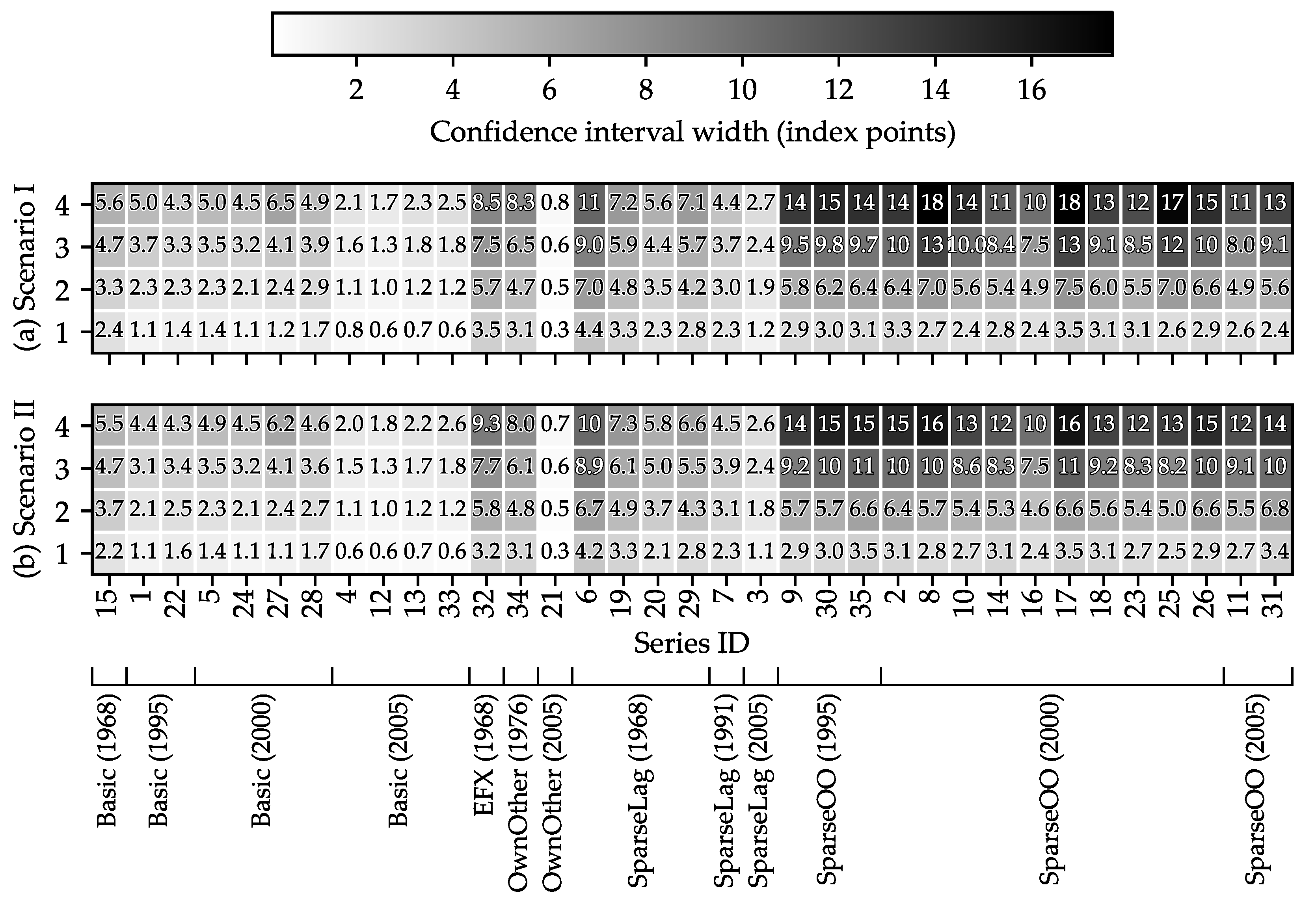
Figure A3.
Widths of the forecast confidence intervals for “curtain-type ventilated facade” (Series ID: 8) and “wallpapering works” (Series ID: 35) under alternative model specifications. The models chosen for the ex ante out-of-sample forecasts, based on their lowest prediction errors (MAPE) in the ex post out-of-sample evaluation period, display relatively wide intervals (Figure A2). The comparison across specifications shows that forecast uncertainty, as reflected in interval width, depends strongly on the chosen model.
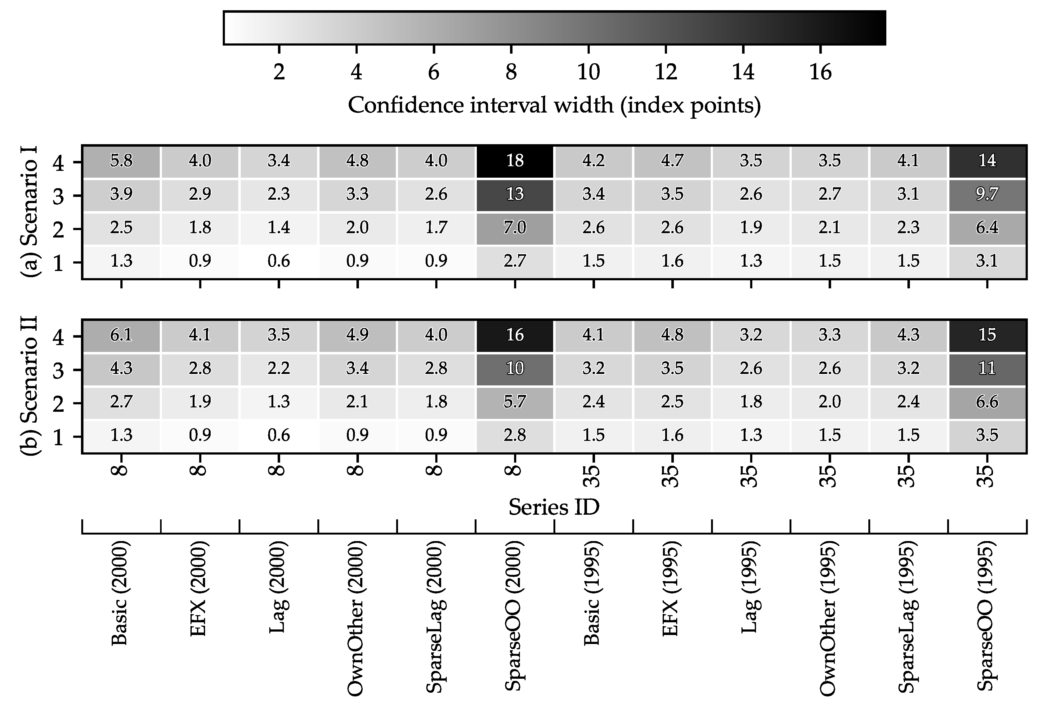
References
- Federal Statistical Office (Statistisches Bundesamt). Number of Building Permits for New Office and Administration Buildings in Germany from 1991 to 2024. In Statista. Available online: https://de.statista.com/statistik/daten/studie/257674/umfrage/baugenehmigungen-fuer-buero-und-verwaltungsgebaeude-in-deutschland/ (accessed on 7 August 2025).
- Federal Statistical Office (Statistisches Bundesamt). Number of Residential and Non-Residential Building Completions in Germany from 2002 to 2024 (in 1,000). In Statista. Available online: https://de.statista.com/statistik/daten/studie/70370/umfrage/baufertigstellungen-wohngebaeude-und-nichtwohngebaeude-seit-1998/ (accessed on 7 August 2025).
- German Construction Industry Association (Hauptverband der Deutschen Bauindustrie). Number of Insolvencies in the Construction Industry in Germany Between 1995 and 2023 (per 10,000 Companies). In Statista. Available online: https://de.statista.com/statistik/daten/studie/152510/umfrage/bau-insolvenzhaeufigkeit-im-branchenvergleich-in-deutschland-seit-1995/ (accessed on 7 August 2025).
- Sommer, H. Projektmanagement im Hochbau: 35 Jahre Innovationen bei Drees & Sommer [Project Management in Building Construction: 35 Years of Innovation at Drees & Sommer], 3rd ed.; Springer: Berlin/Heidelberg, Germany, 2009. (In German) [Google Scholar] [CrossRef] [Scilit]
- Scholz, S.; Wellner, K.; Zeitner, R.; Schramm, C.; Hackel, M.; Hackel, A. Architekturpraxis Bauökonomie: Grundlagenwissen für die Planungs-, Bau- und Nutzungsphase sowie Wirtschaftlichkeit im Planungsbüro [Architectural Practice Construction Economics: Basic Knowledge for the Planning, Construction and Usage Phases and Economic Efficiency in the Design Office], 2nd ed.; Springer Vieweg: Wiesbaden, Germany, 2019. (In German) [Google Scholar] [CrossRef] [Scilit]
- Siemon, K.D.; Siemon, A. Baukostenplanung und -Steuerung: Bei Neu- und Umbauten [Construction Cost Planning and Control: For New Construction and Refurbishment], 7th ed.; Springer Vieweg: Wiesbaden, Germany, 2021. (In German) [Google Scholar] [CrossRef] [Scilit]
- Shane, J.S.; Molenaar, K.R.; Anderson, S.; Schexnayder, C. Construction Project Cost Escalation Factors. J. Manag. Eng. 2009, 25, 221–229. [Google Scholar] [CrossRef] [Scilit]
- Blair, A.N.; Lye, L.M.; Campbell, W.J. Forecasting construction cost escalation. Can. J. Civ. Eng. 1993, 20, 602–612. [Google Scholar] [CrossRef] [Scilit]
- German Institute for Standardisation e. V. DIN 276:2018-12 Building Costs; DIN Media GmbH: Berlin, Germany, 2018. [Google Scholar]
- Williams, T.P. Predicting Changes in Construction Cost Indexes Using Neural Networks. J. Constr. Eng. Manag. 1994, 120, 306–320. [Google Scholar] [CrossRef] [Scilit]
- Ashuri, B.; Lu, J. Time Series Analysis of ENR Construction Cost Index. J. Constr. Eng. Manag. 2010, 136, 1227–1237. [Google Scholar] [CrossRef] [Scilit]
- Moon, S.; Chi, S.; Kim, D.Y. Predicting Construction Cost Index Using the Autoregressive Fractionally Integrated Moving Average Model. J. Manag. Eng. 2018, 34, 04017063. [Google Scholar] [CrossRef] [Scilit]
- Shahandashti, S.M.; Ashuri, B. Forecasting Engineering News-Record Construction Cost Index Using Multivariate Time Series Models. J. Constr. Eng. Manag. 2013, 139, 1237–1243. [Google Scholar] [CrossRef] [Scilit]
- Xu, J.; Moon, S. Stochastic Forecast of Construction Cost Index Using a Cointegrated Vector Autoregression Model. J. Manag. Eng. 2013, 29, 10–18. [Google Scholar] [CrossRef] [Scilit]
- Zhao, L.; Mbachu, J.; Liu, Z. Modelling Residential Building Costs in New Zealand: A Time-Series Transfer Function Approach. Math. Probl. Eng. 2020, 2020, 7028049. [Google Scholar] [CrossRef] [Scilit]
- Nicholson, W.B.; Matteson, D.S.; Bien, J. VARX-L: Structured Regularization for Large Vector Autoregressions with Exogenous Variables. Int. J. Forecast. 2017, 33, 627–651. [Google Scholar] [CrossRef] [Scilit]
- Moon, T.; Shin, D.H. Forecasting Construction Cost Index Using Interrupted Time-Series. KSCE J. Civ. Eng. 2018, 22, 1626–1633. [Google Scholar] [CrossRef] [Scilit]
- Zhao, L.; Mbachu, J.; Zhang, H. Forecasting Residential Building Costs in New Zealand Using a Univariate Approach. Int. J. Eng. Bus. Manag. 2019, 11, 1847979019880061. [Google Scholar] [CrossRef] [Scilit]
- Moon, T.; Shin, D.H. Forecasting Model of Construction Cost Index Based on VECM with Search Query. KSCE J. Civ. Eng. 2018, 22, 2726–2734. [Google Scholar] [CrossRef] [Scilit]
- Choi, C.-Y.; Ryu, K.R.; Shahandashti, M. Predicting City-Level Construction Cost Index Using Linear Forecasting Models. J. Constr. Eng. Manag. 2021, 147, 04020158. [Google Scholar] [CrossRef] [Scilit]
- Wang, J.; Ashuri, B. Predicting ENR Construction Cost Index Using Machine-Learning Algorithms. Int. J. Constr. Educ. Res. 2016, 13, 47–63. [Google Scholar] [CrossRef] [Scilit]
- Dong, J.; Chen, Y.; Guan, G. Cost Index Predictions for Construction Engineering Based on LSTM Neural Networks. Adv. Civ. Eng. 2020, 2020, 6518147. [Google Scholar] [CrossRef] [Scilit]
- Al Kailani, H.; Sweis, G.J.; Sammour, F.; Maaitah, W.O.; Sweis, R.J.; Alkailani, M. Predicting Construction Cost Index Using Fuzzy Logic and Machine Learning in Jordan. Constr. Innov. Inf. Process Manag. 2025, 25, 1479–1500. [Google Scholar] [CrossRef] [Scilit]
- Alzara, M.; Gihad, N.; Abdou, H.; Soltan, A.; Hilal, A.; Ehab, A. Macroeconomic-aware forecasting of construction costs in developing countries: Using gated recurrent unit and long short-term memory deep learning framework. PLoS ONE 2025, 20, e0333189. [Google Scholar] [CrossRef] [Scilit]
- Zhang, R.; Ashuri, B.; Deng, Y. A Novel Method for Forecasting Time Series Based on Fuzzy Logic and Visibility Graph. Adv. Data Anal. Classif. 2017, 11, 759–783. [Google Scholar] [CrossRef] [Scilit]
- Zhang, R.; Ashuri, B.; Shyr, Y.; Deng, Y. Forecasting Construction Cost Index Based on Visibility Graph: A Network Approach. Phys. A Stat. Mech. Appl. 2018, 493, 239–252. [Google Scholar] [CrossRef] [Scilit]
- Mao, S.; Xiao, F. A Novel Method for Forecasting Construction Cost Index Based on Complex Network. Phys. A Stat. Mech. Appl. 2019, 527, 121306. [Google Scholar] [CrossRef] [Scilit]
- Hu, Y.; Xiao, F. A Novel Method for Forecasting Time Series Based on Directed Visibility Graph and Improved Random Walk. Phys. A Stat. Mech. Appl. 2022, 594, 127029. [Google Scholar] [CrossRef] [Scilit]
- Hu, Y.; Xiao, F. An Efficient Forecasting Method for Time Series Based on Visibility Graph and Multi-Subgraph Similarity. Chaos Solitons Fractals 2022, 160, 112243. [Google Scholar] [CrossRef] [Scilit]
- Hu, Y.; Xiao, F. Network Self Attention for Forecasting Time Series. Appl. Soft Comput. J. 2022, 124, 109092. [Google Scholar] [CrossRef] [Scilit]
- Hu, Y.; Xiao, F. Time-Series Forecasting Based on Fuzzy Cognitive Visibility Graph and Weighted Multisubgraph Similarity. IEEE Trans. Fuzzy Syst. 2023, 31, 1281–1293. [Google Scholar] [CrossRef] [Scilit]
- Zhan, T.; Xiao, F. A Novel Weighted Approach for Time Series Forecasting Based on Visibility Graph. Pattern Recognit. 2024, 155, 110720. [Google Scholar] [CrossRef] [Scilit]
- Cao, M.-T.; Cheng, M.-Y.; Wu, Y.-W. Hybrid Computational Model for Forecasting Taiwan Construction Cost Index. J. Constr. Eng. Manag. 2015, 141, 04014089. [Google Scholar] [CrossRef] [Scilit]
- Xie, S.; Fang, J. Prediction of Construction Cost Index Based on Multi Variable Grey Neural Network Model. Int. J. Inf. Syst. Change Manag. 2018, 10, 209–226. [Google Scholar] [CrossRef] [Scilit]
- Kim, S.; Choi, C.-Y.; Shahandashti, M.; Ryu, K.R. Improving Accuracy in Predicting City-Level Construction Cost Indices by Combining Linear ARIMA and Nonlinear ANNs. J. Manag. Eng. 2022, 38, 04021093. [Google Scholar] [CrossRef] [Scilit]
- Myrvang, R.; Liu, C.-Y.A. Beyond Traditional Methods: Enhancing Cost Escalation Forecasting in Commercial Construction amid Economic Turbulence. J. Constr. Eng. Manag. 2025, 151, 04024201. [Google Scholar] [CrossRef] [Scilit]
- Hwang, S. Dynamic Regression Models for Prediction of Construction Costs. J. Constr. Eng. Manag. 2009, 135, 360–367. [Google Scholar] [CrossRef] [Scilit]
- Hwang, S. Time Series Models for Forecasting Construction Costs Using Time Series Indexes. J. Constr. Eng. Manag. 2011, 137, 656–662. [Google Scholar] [CrossRef] [Scilit]
- Elfahham, Y. Estimation and Prediction of Construction Cost Index Using Neural Networks, Time Series, and Regression. Alex. Eng. J. 2019, 58, 499–506. [Google Scholar] [CrossRef] [Scilit]
- Aslam, B.; Maqsoom, A.; Inam, H.; Basharat, M.U.; Ullah, F. Forecasting Construction Cost Index through Artificial Intelligence. Societies 2023, 13, 219. [Google Scholar] [CrossRef] [Scilit]
- Aydinli, S. Impact of Unexpected Conditions on Construction Cost Forecasting Performance: Evidence from Europe. Constr. Manag. Econ. 2024, 42, 787–801. [Google Scholar] [CrossRef] [Scilit]
- Lin, Y.-C.; Marzuki, J.; Lee, C.L. Portfolio Construction Strategy for Global Non-Listed Office Real Estate Investment in Interest Rate Cycles. Buildings 2025, 15, 3570. [Google Scholar] [CrossRef] [Scilit]
- Lin, Y.; Lee, C.L.; Newell, G. Varying interest rate sensitivity of different property sectors: Cross-country evidence from REITs. J. Prop. Invest. Finance 2022, 40, 68–98. [Google Scholar] [CrossRef] [Scilit]
- Marzuki, J. Analysis of the Performance and Diversification Benefits of the South Africa Commercial Real Estate Market. J. Real Estate Lit. 2018, 26, 291–311. [Google Scholar] [CrossRef] [Scilit]
- Karshenas, S. Predesign Cost Estimating Method for Multistory Buildings. J. Constr. Eng. Manag. 1984, 110, 79–86. [Google Scholar] [CrossRef] [Scilit]
- Li, H.; Shen, Q.P.; Love, P.E.D. Cost modelling of office buildings in Hong Kong: An exploratory study. Facilities 2005, 23, 438–452. [Google Scholar] [CrossRef] [Scilit]
- Alshamrani, O.S. Initial cost forecasting model of mid-rise green office buildings. J. Asian Archit. Build. Eng. 2020, 19, 613–625. [Google Scholar] [CrossRef] [Scilit]
- Chen, G.; Zheng, S.; He, X.; Liang, X.; Liao, X. Machine Learning-Based Cost Estimation Models for Office Buildings. Buildings 2025, 15, 1802. [Google Scholar] [CrossRef] [Scilit]
- Starczyk-Kołbyk, A.; Jędras, I. Integrated Risk Assessment in Construction Contracts: Comparative Evaluation of Risk Matrix and Monte Carlo Simulation on a High-Rise Office Building Project. Appl. Sci. 2025, 15, 9371. [Google Scholar] [CrossRef] [Scilit]
- Federal Statistical Office (Statistisches Bundesamt). Construction Price Indices for Buildings in Germany (GENESIS-Online Database, Table 61261-0002). Available online: https://www-genesis.destatis.de/datenbank/online/statistic/61261/table/61261-0002/search/s/YmF1cHJlaXNpbmRpemVz (accessed on 7 August 2025).
- Federal Statistical Office (Statistisches Bundesamt). Construction Price Indices—Weighting Schemes 2021. Statistical Report, Published on 10 July 2024. Wiesbaden, Germany, 2024. Available online: https://www.destatis.de (accessed on 22 September 2025).
- Federal Statistical Office (Statistisches Bundesamt). Qualitätsbericht: Preisindizes für die Bauwirtschaft—Statistik der Bauleistungspreise; Statistisches Bundesamt: Wiesbaden, Germany, 2012; Available online: https://www.destatis.de/DE/Methoden/Qualitaet/Qualitaetsberichte/Preise/bauleistungspreise.pdf?__blob=publicationFile (accessed on 7 August 2025).
- Federal Statistical Office, Germany. Germany, Prices, Consumer Prices, All Items, Total, Index, 2020 = 100 (Mnemonic: BDCONPRCF; RIC: aDECPI), Monthly Data, Jun 1948–Oct 2025. Data Retrieved via LSEG Datastream (London Stock Exchange Group). Available online: https://www.lseg.com/en/data-analytics/products/datastream-macroeconomic-analysis (accessed on 10 September 2025).
- Ashuri, B.; Shahandashti, S.M.; Lu, J. Empirical tests for identifying leading indicators of ENR Construction Cost Index. Constr. Manag. Econ. 2012, 30, 917–927. [Google Scholar] [CrossRef] [Scilit]
- Nguyen, T.P.; Nguyen, L.H.T.T.; Quyen. Critical Factors Affecting Construction Price Index: An Integrated Fuzzy Logic and Analytical Hierarchy Process. J. Asian Financ. Econ. Bus. 2020, 7, 197–204. [Google Scholar] [CrossRef] [Scilit]
- Asamoah, R.O.; Baiden, B.K.; Nani, G.; Kissi, E. Review of exogenous economic indicators influencing construction industry. Adv. Civ. Eng. 2019, 2019, 6073289. [Google Scholar] [CrossRef] [Scilit]
- Leamer, E. Housing Is the Business Cycle; National Bureau of Economic Research: Cambridge, MA, USA, 2007. [Google Scholar] [CrossRef] [Scilit]
- Shahandashti, S.M.; Ashuri, B. Highway Construction Cost Forecasting Using Vector Error Correction Models. J. Manag. Eng. 2016, 32, 04015040. [Google Scholar] [CrossRef] [Scilit]
- Federal Statistical Office (Statistisches Bundesamt, Destatis). Volkswirtschaftliche Gesamtrechnungen—Bruttoinlandsprodukt (Table 81000-118; Quarterly); Quarterly Publication: Wiesbaden, Germany, 2025; Article Number 2180120253225; Available online: https://www.destatis.de/DE/Themen/Wirtschaft/Volkswirtschaftliche-Gesamtrechnungen-Inlandsprodukt/_inhalt.html#_zrqiagoxq (accessed on 22 August 2025).
- Organization for Economic Co-Operation and Development. Interest Rates: 3-Month or 90-Day Rates and Yields: Interbank Rates: Total for Germany [IR3TIB01DEM156N], Retrieved from FRED, Federal Reserve Bank of St. Louis. Available online: https://fred.stlouisfed.org/series/IR3TIB01DEM156N (accessed on 10 September 2025).
- Johansen, S. Likelihood-Based Inference in Cointegrated Vector Autoregressive Models; Oxford University Press: Oxford, UK, 1995. [Google Scholar]
- Lütkepohl, H. New Introduction to Multiple Time Series Analysis; Springer: Berlin, Germany; New York, NY, USA, 2005. [Google Scholar] [CrossRef]
- Aggarwal, C.C. Outlier Analysis, 2nd ed.; Springer Nature: Cham, Switzerland, 2017; ISBN 978-3-319-47578-3. [Google Scholar]
- Lee, K.; Jeong, Y.; Joo, S.; Yoon, Y.S.; Han, S.; Baik, H. Outliers in financial time series data: Outliers, margin debt, and economic recession. Mach. Learn. Appl. 2022, 10, 100420. [Google Scholar] [CrossRef] [Scilit]
- Lartey, C.; Liu, J.; Asamoah, R.K.; Greet, C.; Zanin, M.; Skinner, W. Effective Outlier Detection for Ensuring Data Quality in Flotation Data Modelling Using Machine Learning (ML) Algorithms. Minerals 2024, 14, 925. [Google Scholar] [CrossRef] [Scilit]
- Stowe, E.J.; Keller, M.R.; Connizzo, B.K. Cellular senescence impairs tendon extracellular matrix remodeling in response to mechanical unloading. Aging Cell 2024, 23, e14278. [Google Scholar] [CrossRef] [Scilit]
- Johansen, S. Estimation and Hypothesis Testing of Cointegration Vectors in Gaussian Vector Autoregressive Models. Econometrica 1991, 59, 1551–1580. [Google Scholar] [CrossRef] [Scilit]
- Lütkepohl, H.; Saikkonen, P.; Trenkler, C. Maximum eigenvalue versus trace tests for the cointegrating rank of a VAR process. In Interdisciplinary Research Project 373: Quantification and Simulation of Economic Processes; SFB 373 Discussion Paper; Humboldt University of Berlin: Berlin, Germany, 2000; Volume 83, Available online: https://nbn-resolving.de/urn:nbn:de:kobv:11-10048091 (accessed on 10 September 2025).
- Hyndman, R.J.; Athanasopoulos, G. Forecasting: Principles and Practice, 3rd ed.; OTexts: Melbourne, Australia, 2021; Available online: https://otexts.com/fpp3/ (accessed on 9 September 2025).
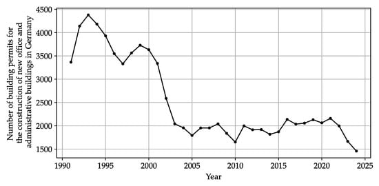
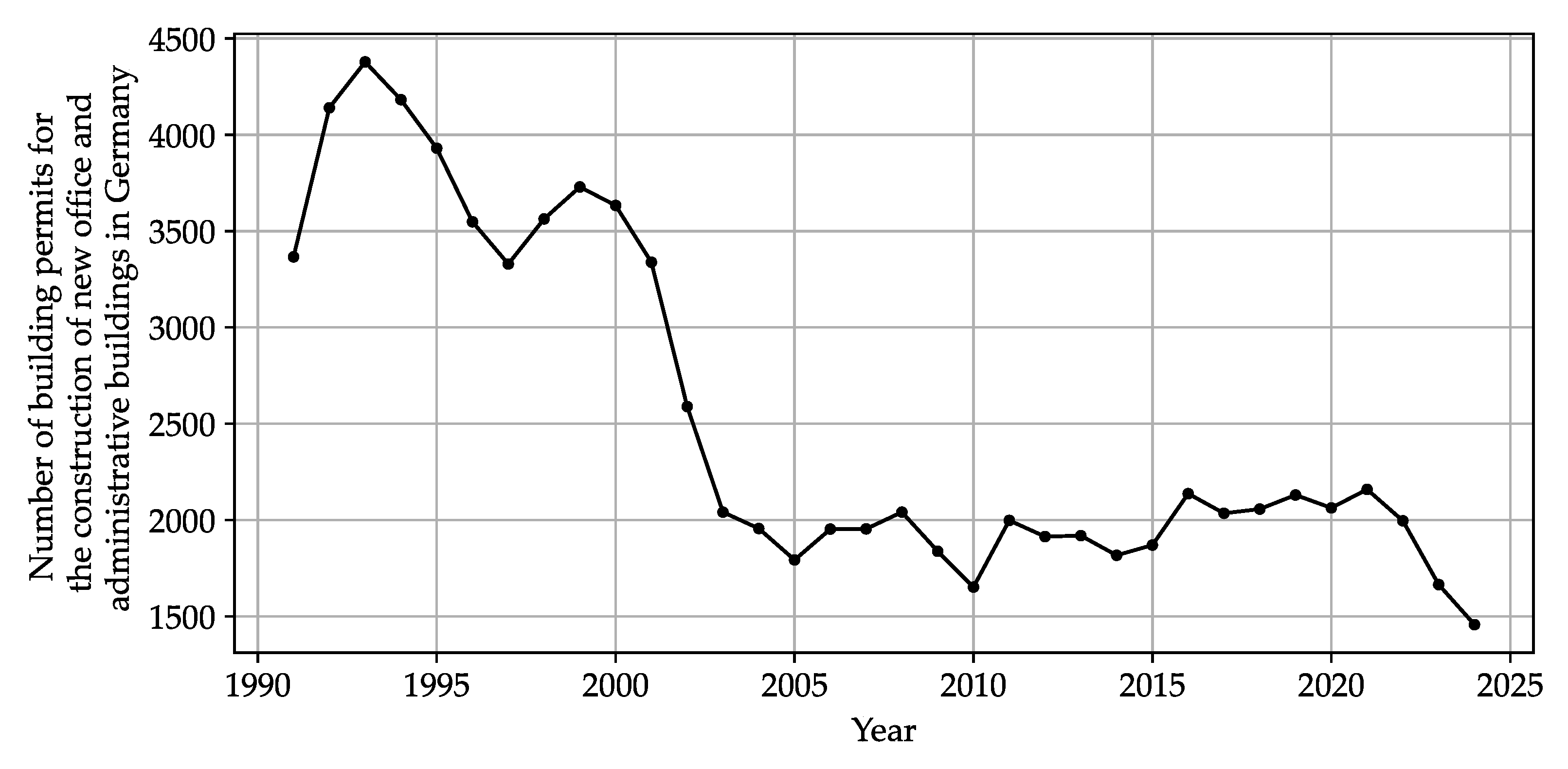
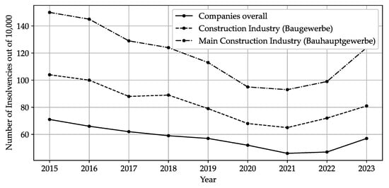
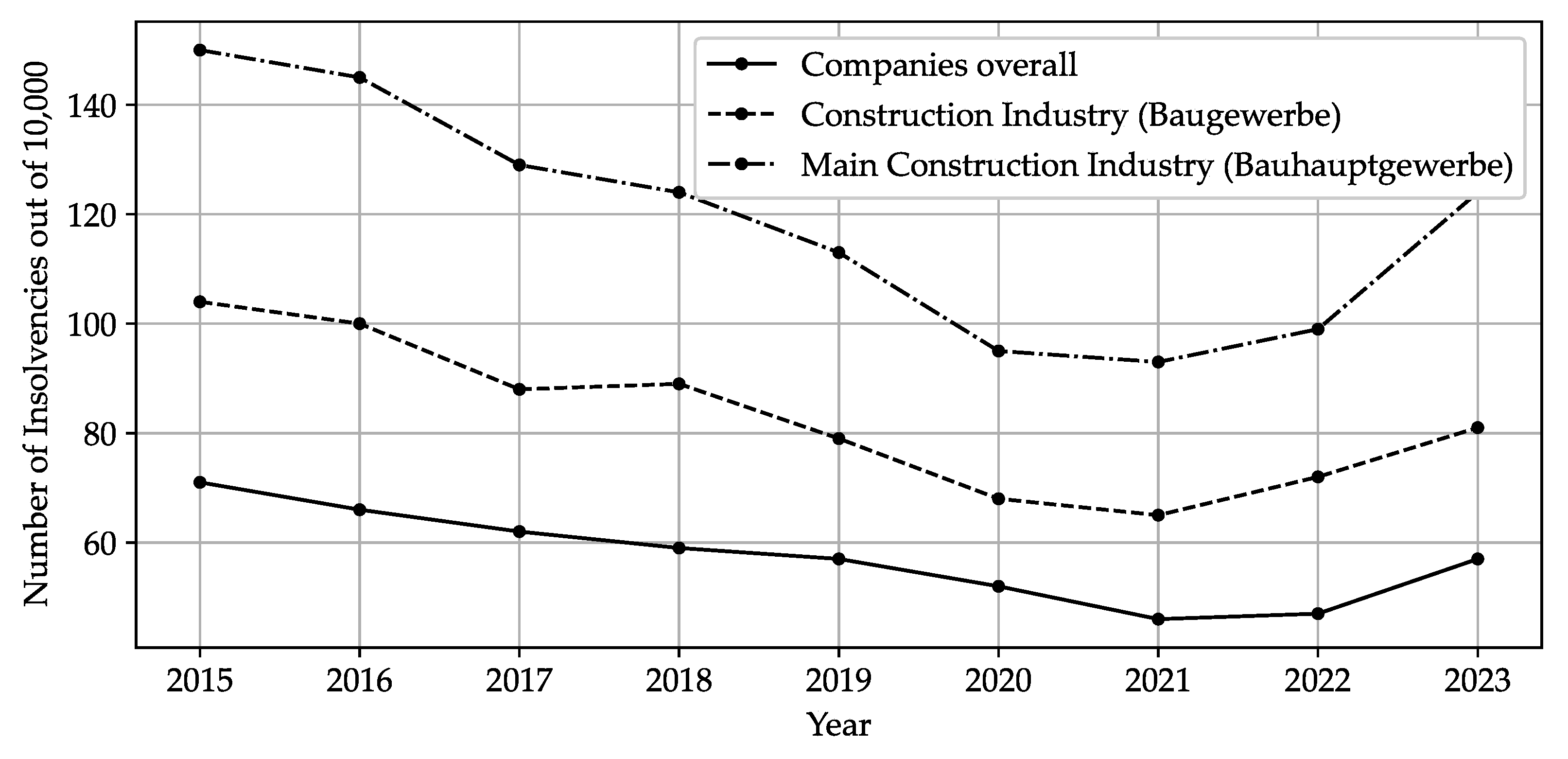
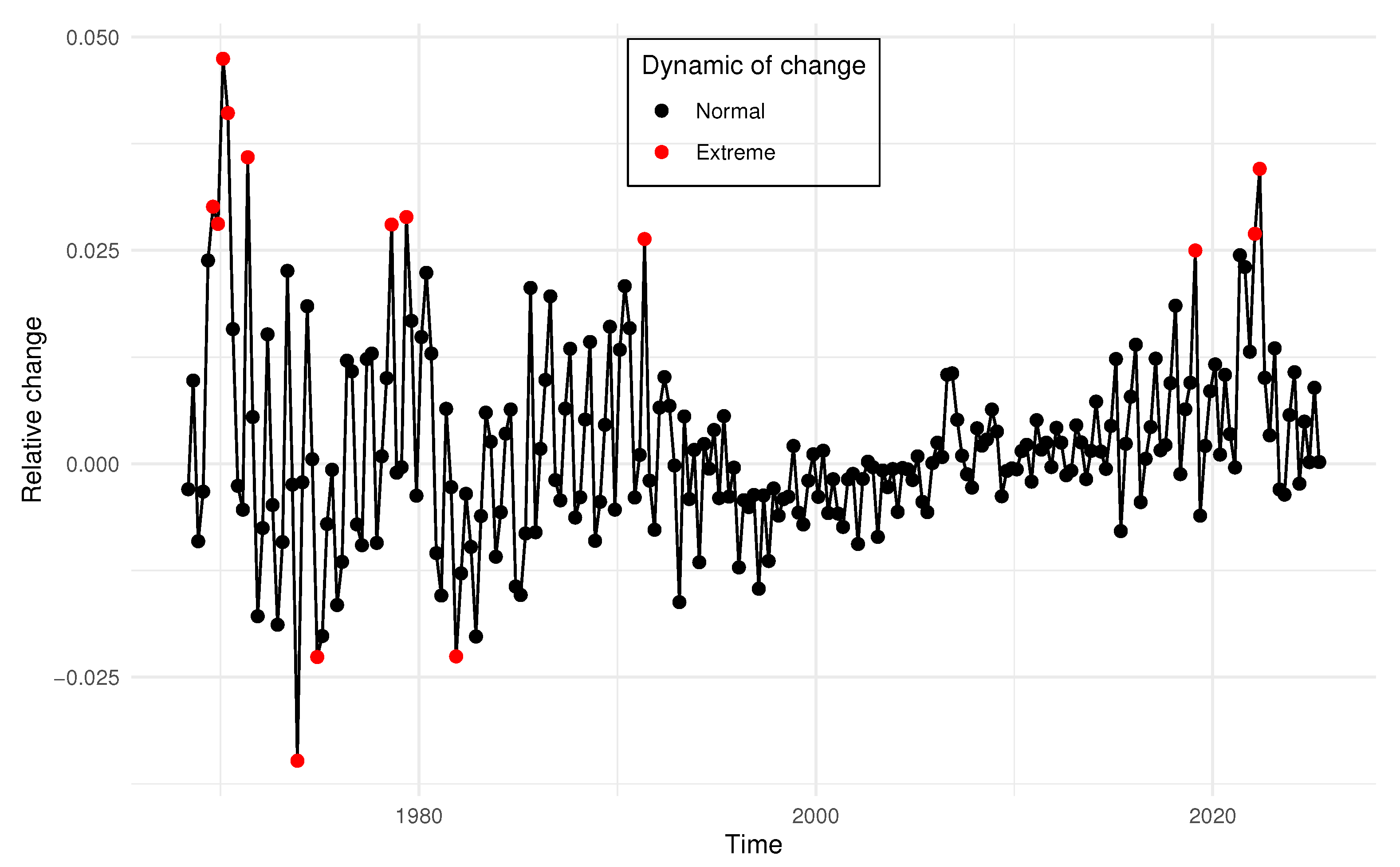
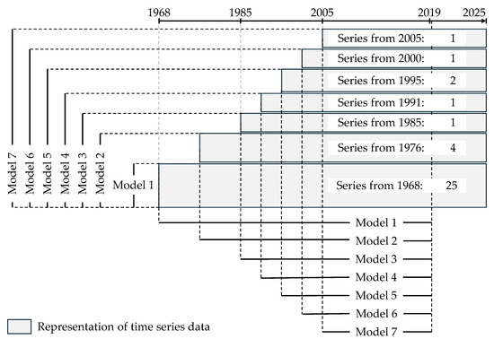
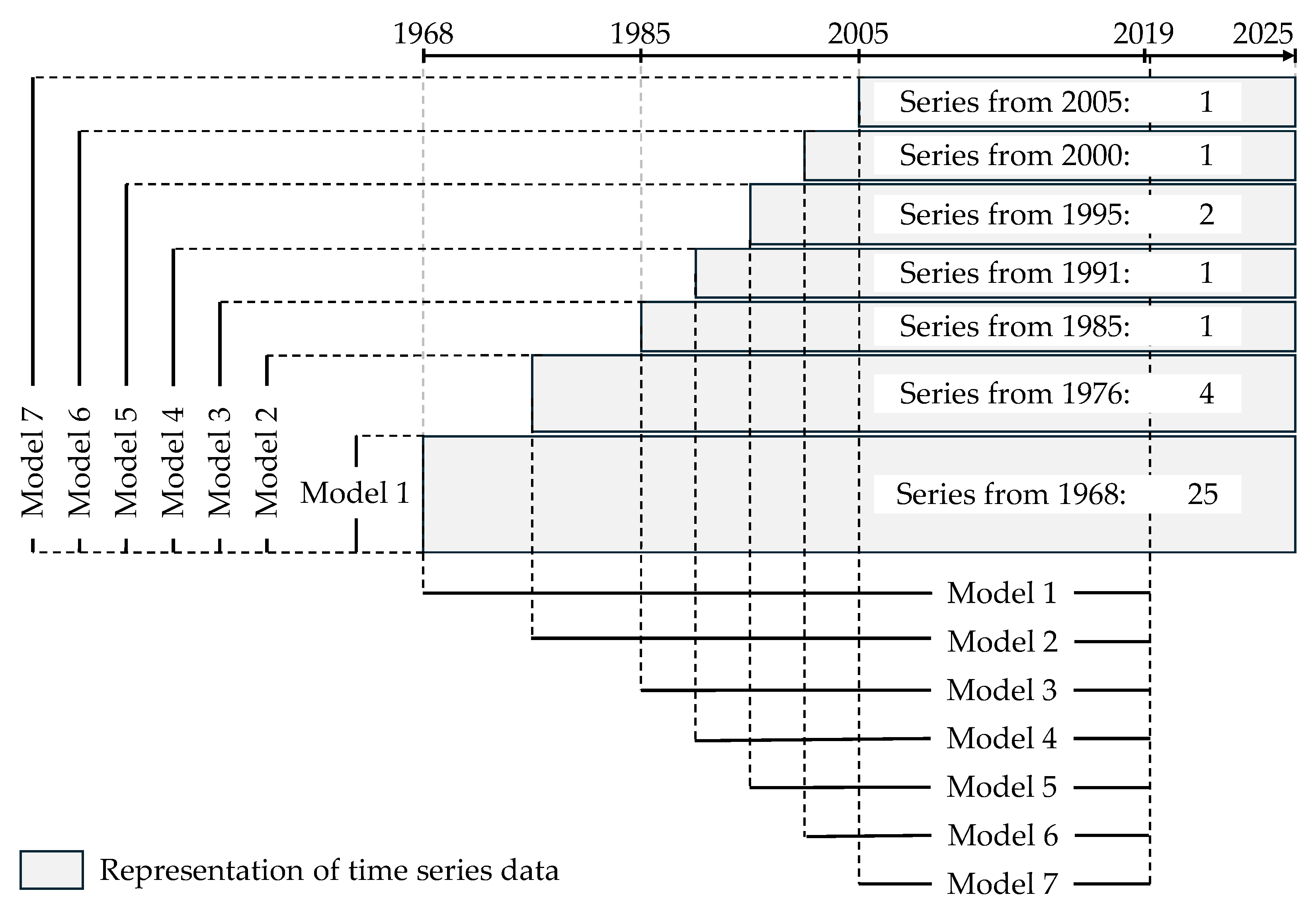
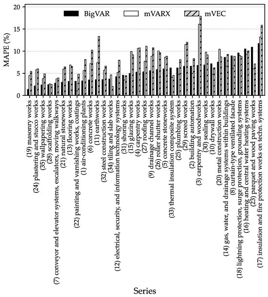
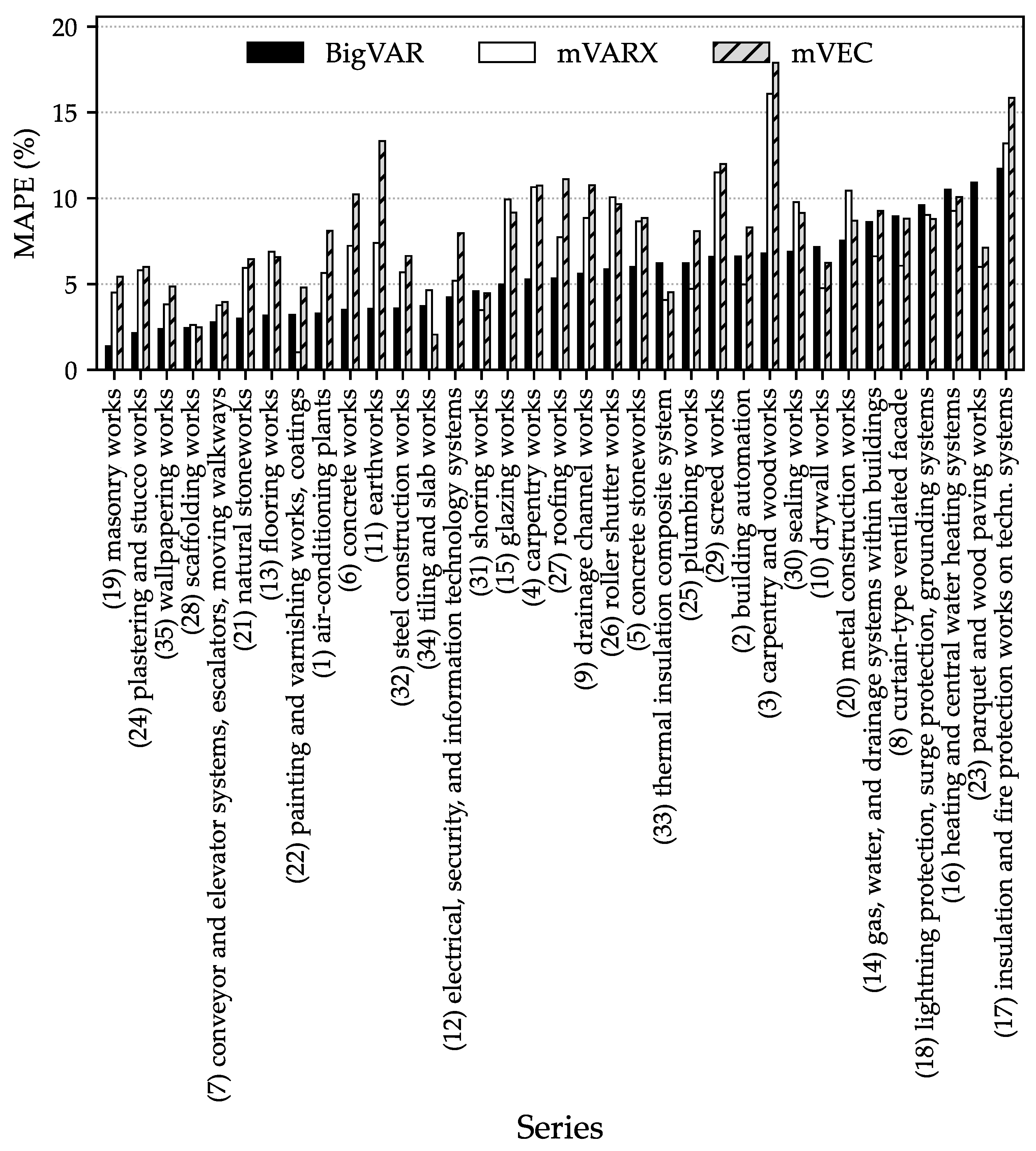
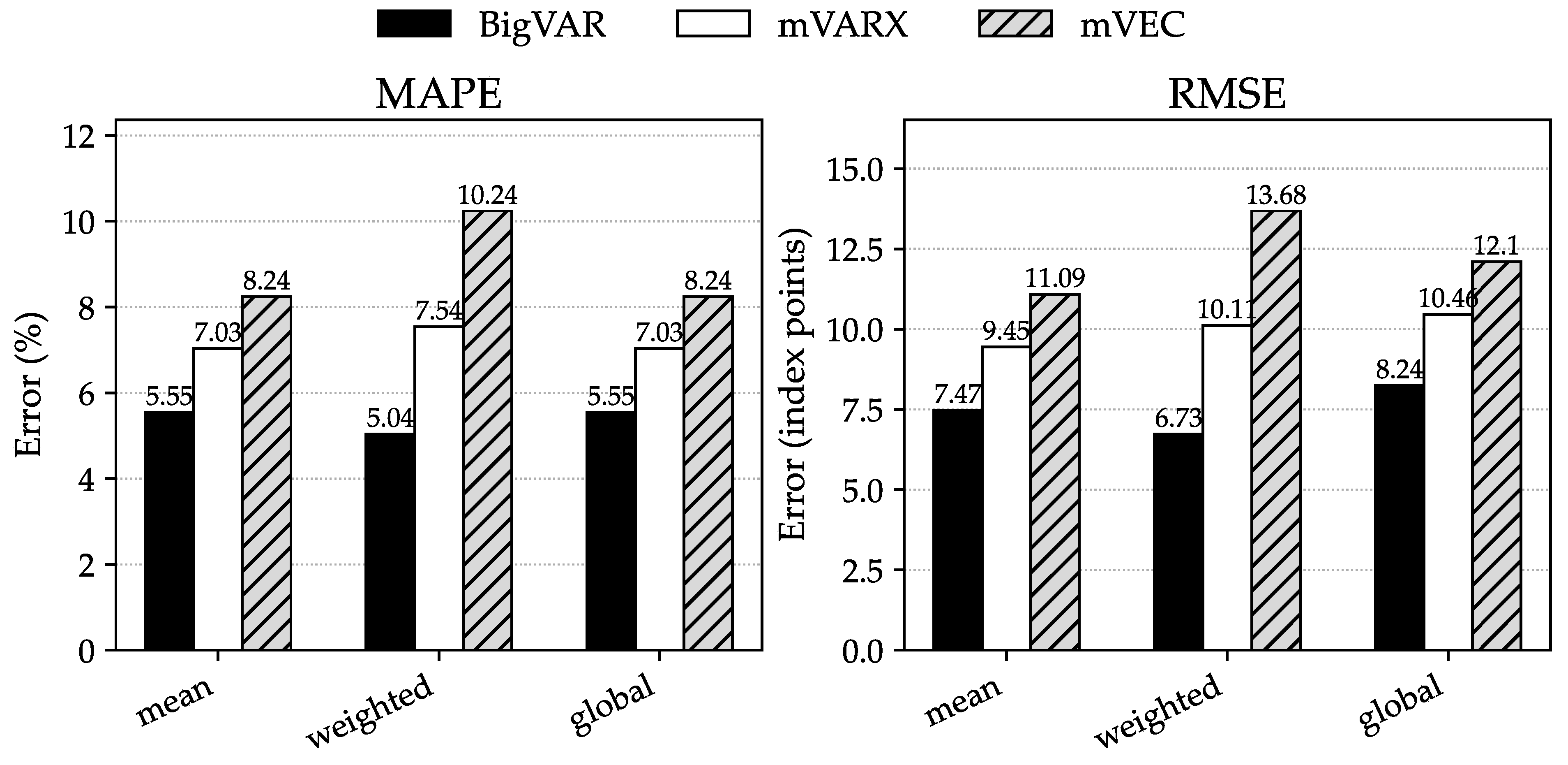
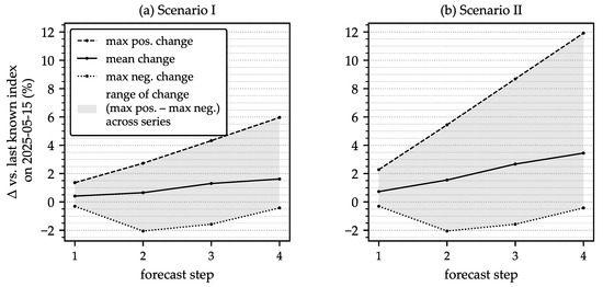
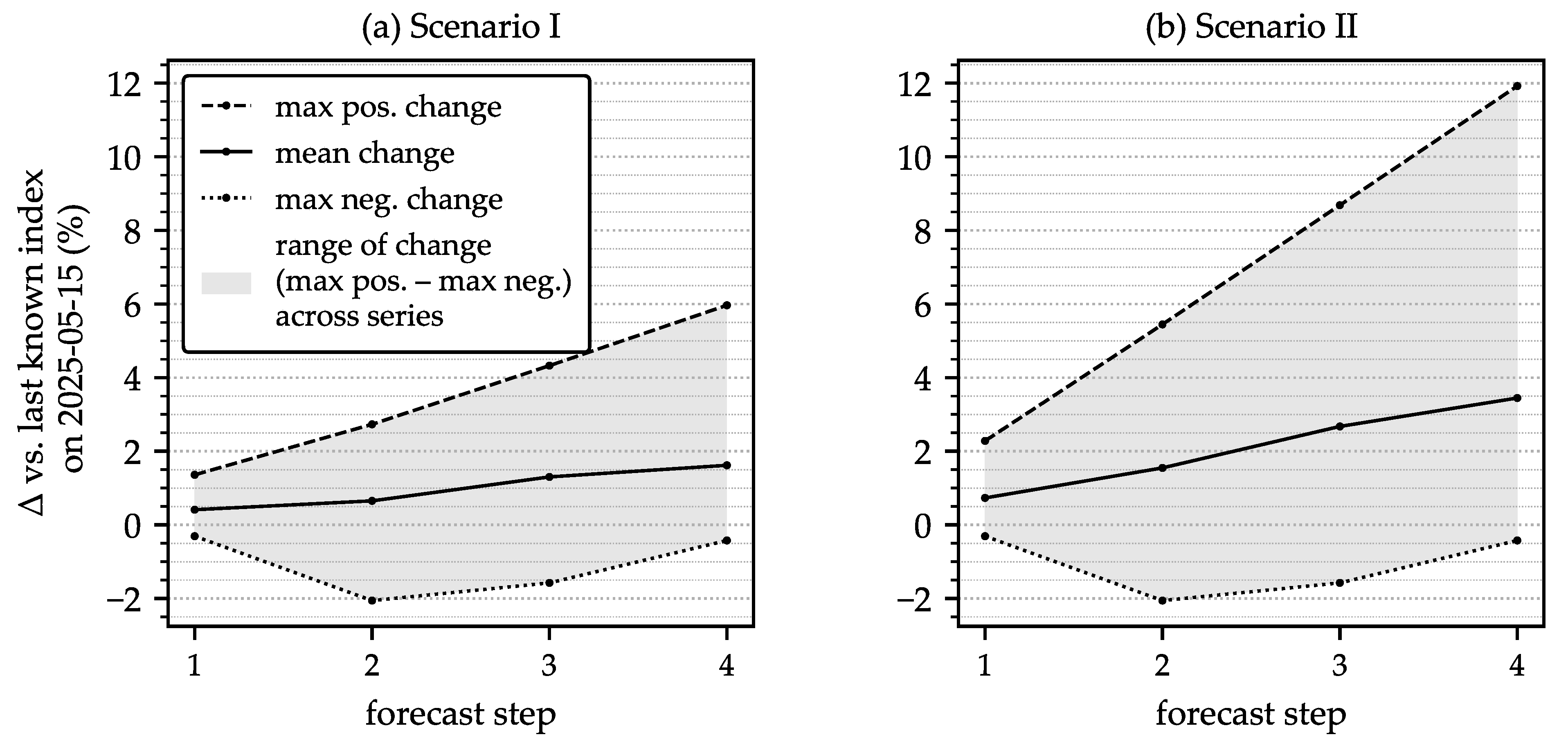
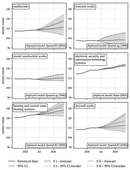
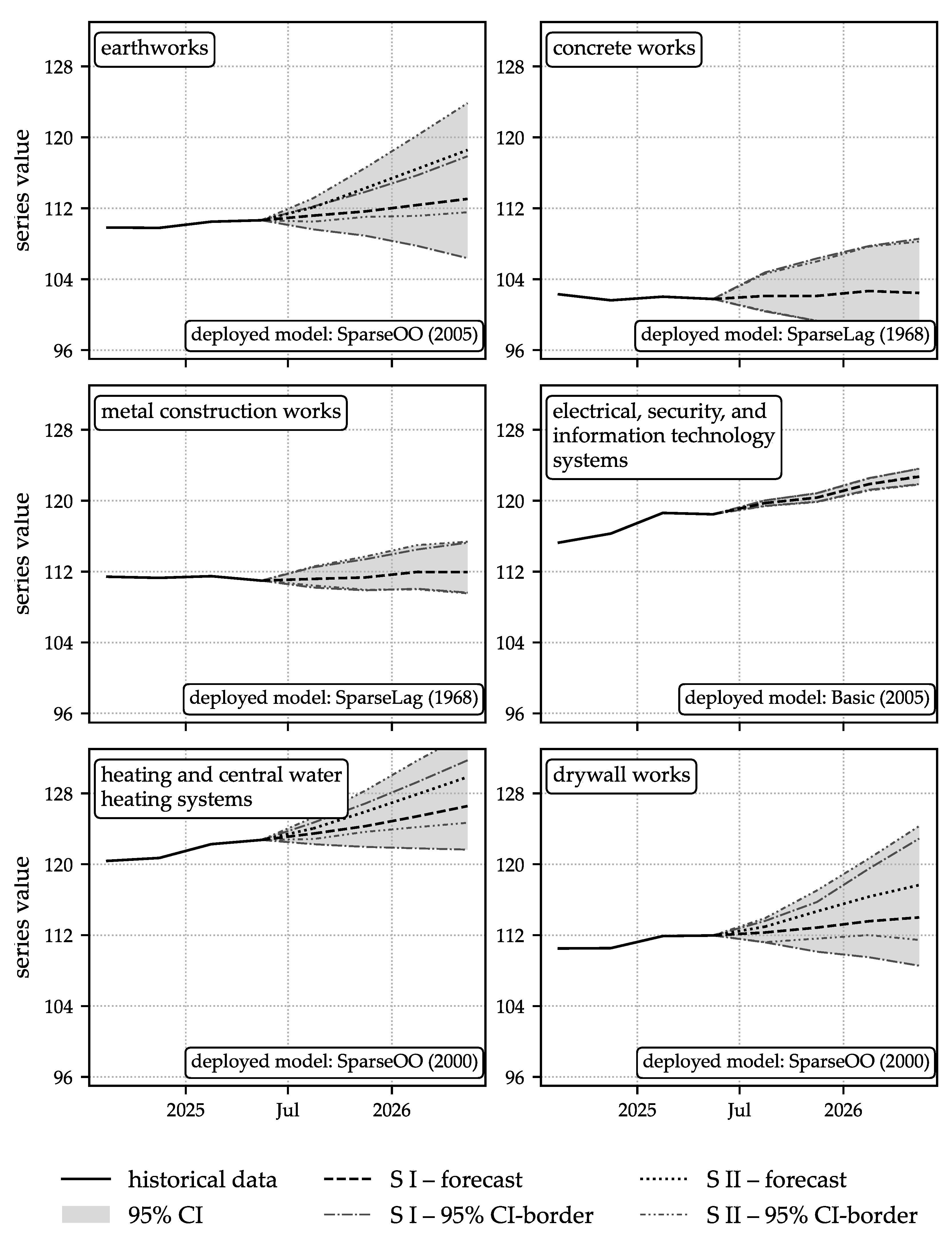
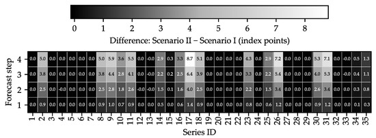
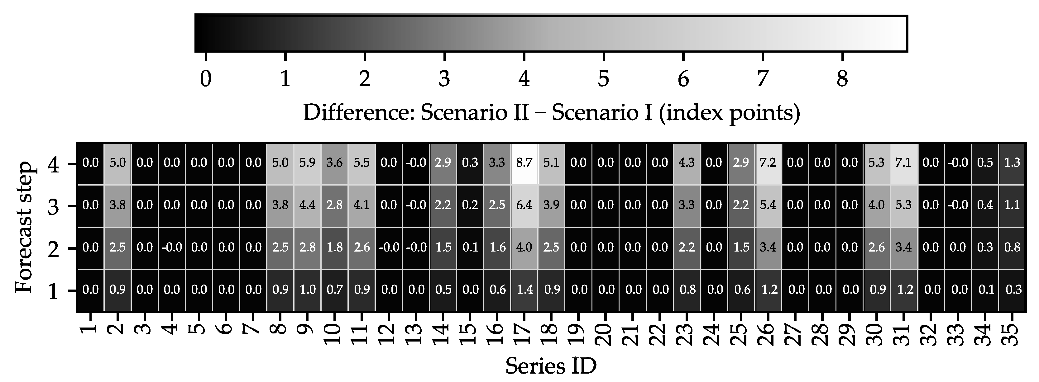
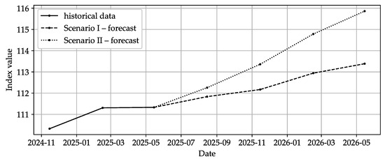
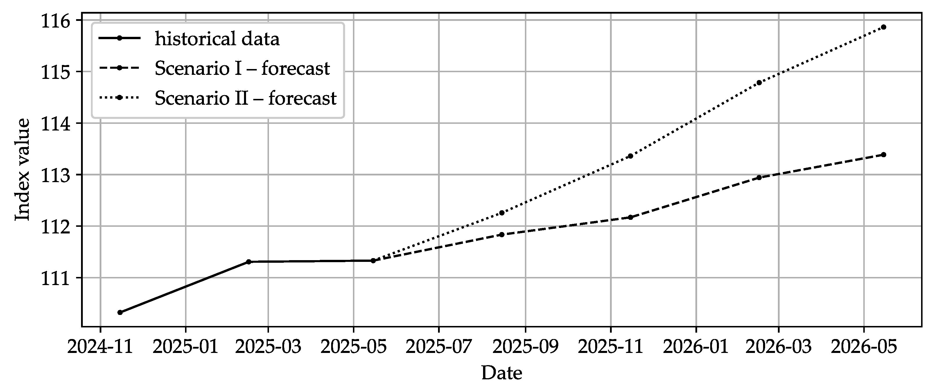
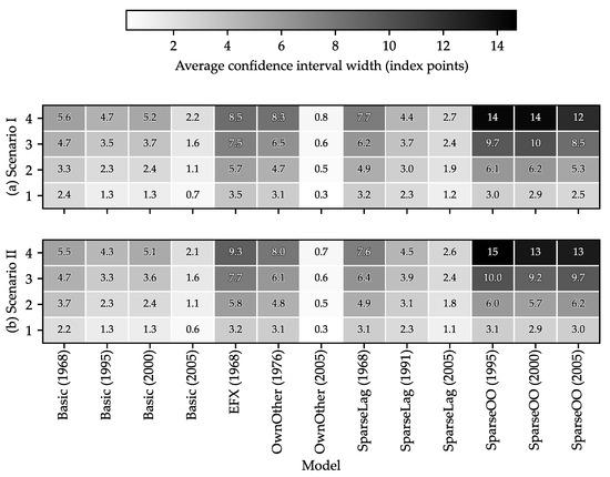
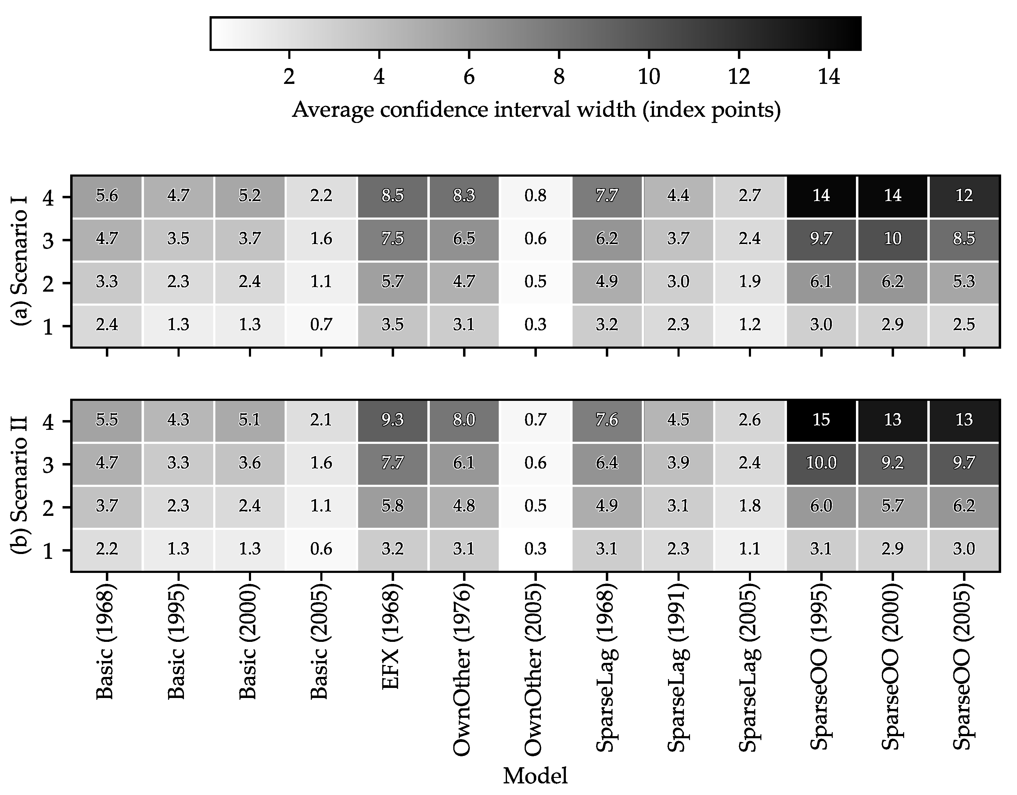

Disclaimer/Publisher’s Note: The statements, opinions and data contained in all publications are solely those of the individual author(s) and contributor(s) and not of MDPI and/or the editor(s). MDPI and/or the editor(s) disclaim responsibility for any injury to people or property resulting from any ideas, methods, instructions or products referred to in the content. |
© 2025 by the authors. Licensee MDPI, Basel, Switzerland. This article is an open access article distributed under the terms and conditions of the Creative Commons Attribution (CC BY) license.