


Abstract
Conventional corrosivity assessment requires gravimetric measurements over exposure periods of at least one year (ISO 9223/9226), limiting rapid maintenance decisions for infrastructure. To address this gap, a predictive model for atmospheric corrosion-induced mass loss in AISI 1020 carbon steel and galvanized steel was developed using images analyzed through artificial neural networks (ANNs). The model was trained on RGB and HSV color-space images from salt-spray and field specimens. Three models were implemented: a YOLOv8-based segmentation network (ANN-1) to isolate corroded regions; a feedforward neural network (ANN-2) to predict mass loss from pixel color histograms; and an extended network (ANN-3) using meteorological variables to classify environmental corrosivity. The models estimated corrosion rates of 1204 ± 202 µm·year−1 for AISI 1020 carbon steel and 61 ± 44 µm·year−1 for galvanized steel in accelerated salt-spray tests, expressed as thickness loss per year, with low mean absolute errors and high R2 values. Applied to transmission towers and substations in Northeast Brazil, the predictions fell within experimental error margins—4.74 ± 1.60 g·year−1 predicted against 4.73 ± 1.61 g·year−1 measured per specimen for AISI 1020 carbon steel at the most aggressive substation. A graphical interface supports maintenance, material-selection, and surface-treatment decisions based on local corrosivity.
1. Introduction
Atmospheric corrosion of metals in tropical regions, such as Brazil, is influenced by various environmental factors, including temperature, humidity, and pollutants. These factors exhibit significant spatial and temporal variability due to the country’s vast territory and proximity to the coast. Such variability leads to the formation of distinct microclimates, each featuring unique corrosive characteristics. Consequently, corrosion rates are not constant and typically follow a multistage pattern: initially increasing and then decreasing as protective corrosion products accumulate. This complexity necessitates the development of accurate predictive models to assess and mitigate corrosion impacts on metallic structures exposed to different atmospheric conditions [1,2,3,4].
Brazil’s power transmission network covered approximately 184,000 km in November 2023, with plans to expand by over 30,000 km by 2027, including an expansion for the coastal region with over 7000 km of the shoreline [5]. However, climate change is intensifying this exposure: for instance, in 2015, 17% of meteorological stations reported shifts in climate zones, with reductions in tropical humid (Af, Am) and temperate (C) climates and expansions of tropical savanna (Aw) and arid (B) climates, particularly in the Northeast and South [6]. These climatic changes accelerate corrosion processes in metallic materials, leading to significant annual losses in engineering, estimated at over $2.5 trillion globally, approximately 3.4% of the global gross domestic product (GDP) [7].
AISI 1020 carbon steel is widely used in large-scale construction due to its favorable mechanical properties and cost-effectiveness. However, it is particularly susceptible to corrosion, especially in aggressive environmental conditions. To mitigate this, protective coatings are often applied, with galvanization being a well-established and effective method. It provides a physical barrier against corrosive agents and cathodic protection, enhancing the material’s durability and extending its service life in various applications [8].
Climate change and increased industrial activity have intensified atmospheric pollutant emissions, leading to higher corrosion rates in metals, necessitating accelerated testing methods, both in laboratories and field settings, to reduce uncertainties [9,10]. To meet these challenges, advanced tools such as dose–response functions [11] and artificial neural networks (ANNs) [12] are being employed to model and predict corrosion processes more effectively.
Advancements in computer vision and artificial ANNs have significantly enhanced the ability to detect and interpret corrosion in metallic materials, evolving from basic image processing to sophisticated algorithms capable of analyzing complex visual data and providing insights comparable to human visual perception, yielding more efficient and accurate methods for monitoring and managing corrosion in various industrial applications [13,14,15,16].
Feedforward Neural Networks (FFNNs) have been extensively explored in computer vision, especially in tasks such as image classification, regression of visual variables, and pattern recognition. Although effective for simple image classification tasks, FFNNs have proven limited for more complex computer vision problems such as object detection and image segmentation; for such tasks, convolutional neural networks (CNNs) are typically employed [15]. CNNs process tensor-structured data, such as images, through hierarchical layers that enable feature extraction from the simplest to the most complex representations, and this architecture underlies the YOLO (You Only Look Once) network [17], which enhances segmentation tasks and object detection by dividing the image into a grid and simultaneously predicting bounding boxes and class probabilities for each region, enabling real-time performance. The YOLOv8 architecture [18] has been widely applied in different contexts [19,20,21] and, more recently, in corrosion detection in metallic structures.
Standard corrosivity assessment methods remain tied to the exposure periods defined by ISO 9223 [22] and ISO 9226 [23], typically at least one year, before a corrosivity class can be assigned with confidence, leaving a gap in rapid, on-demand assessment that constrains how quickly asset managers can respond to newly installed structures or changing environmental conditions. A visual inspection of metallic materials in the field, combined with ANNs, has proven to be an effective technique for assessing corrosion in energy transmission towers [24], offering a faster alternative to these standardized procedures. This approach utilizes historical data on corrosive processes and environmental conditions, along with photographic images of aged metals from both field and laboratory settings, to train the ANN. This methodology is particularly advantageous due to the challenges associated with removing metallic materials for laboratory testing and the time required to diagnose critical degradation conditions. Furthermore, it enables prompt determination of the need for maintenance interventions, component replacements, or enhancements in surface protection.
1.1. Image Processing
Naturally, visual inspection is one of the primary procedures for assessing the corrosion process and its degradation effects. Consequently, computational methodologies have been developed to compile and interpret such visual information from local images. In this regard, the first strategy employed the natural red, green, and blue (RGB) color space, which is the standard image format. However, due to the limited information provided by this space, other color spaces were explored.
The hue, saturation, and value (HSV) color space was the first alternative utilized [25]. Unlike RGB, the HSV color space provides adjustable parameters that allow differentiation between corroded and non-corroded pixels. Since then, the HSV has been regularly applied in this context [16,26,27], often complemented by texture analysis to further enhance image-based corrosion detection [16,26,27,28], including the exploration of surface patterns and irregularities [29], which can add more information from the images and offer additional evidence of corrosion.
1.2. Artificial Neural Network for Corrosion
After extracting image-derived information, various computational methods can be applied to process and interpret the data. Alongside the traditional corrosivity classification approach established by ABNT NBR 14643 [30], ANNs have emerged as a powerful complementary tool. Early applications of ANNs to the prediction of atmospheric corrosion demonstrated the technique’s feasibility, including a foundational study on low-carbon steel, copper, and aluminum corrosion rates along a power transmission line in equatorial Brazil [31]. Subsequent works included the prediction of corrosion rates in metal pipes [32] and an application to carbon steel in Taiwanese industrial zones [33], both using multi-layered perceptron (MLP) architectures to predict the corrosion rate directly. However, neither study used images as ANN inputs; the first relied on material compositions, pH, flow rate, and temperature, and the second used only the parameters established by ABNT NBR 14643 [30]. Since then, MLP-based ANNs have remained a widely used architecture [34,35,36].
Only recently have approaches emerged that effectively use images as direct inputs to the model, enabled by increasingly available computational power and deeper, more effective deep learning (DL) architectures. Using such DL models, Atha & Jahanshahi [26] evaluated texture extraction and color spaces across multiple CNN architectures to determine the best configuration for the prediction task. Similarly, Yin et al. [37] demonstrated that, despite the challenge of creating the dataset and training the network from scratch, DL models can learn and generalize effectively.
Metaheuristic approaches have also been explored: Liao & Lee [38] used K-means clustering for bridge rust identification; Bondada et al. [39] proposed a similar approach to estimate the total corroded area; Hoang & Tran [27] developed a hybrid approach using the Support Vector Machine (SVM) optimized by the differential flower pollination (DFP) algorithm; Hoang [28] used the history-based adaptive differential evolution with linear population size (LSHADE) metaheuristic for multilevel image thresholding; and Zeraati et al. [40] applied the Genetic Algorithm (GA) to determine the corrosion behavior of Ni-Zn coatings. For cross-sectional estimation, Wu et al. [41] estimated corrosion in power-system grounding electrodes using a Recurrent Neural Network (RNN) with soil environmental parameters as input features, while Lv et al. [42] employed a 3D scanning method to characterize the cross-section morphology of rusted steel, comparing the particle swarm optimization support vector machine (PSO-SVM) and the grid search support vector machine (GS-SVM).
ANNs can also be applied to pitting detection (punctual corrosion that directly impacts the mechanical strength of AISI 1020 carbon steel columns) [43]. More recently, advances in deep learning have extended these capabilities to large-scale infrastructure assessment, including power transmission towers, where image-based corrosion monitoring offers a non-invasive alternative to traditional sampling approaches [24,44].
None of the studies reviewed above combines the three elements pursued here. The image-based approaches—Atha and Jahanshahi [26], Yin et al. [37], Liao and Lee [38], Bondada et al. [39], Hoang and Tran [27], and Hoang [28]—detect, segment, or rate corrosion severity from photographs, but stop short of estimating a quantitative mass-loss or corrosion-rate value. The studies that do predict a numerical corrosion rate—Kenny et al. [31], Abdullah et al. [32], Lin et al. [33], Zeraati et al. [40], Wu et al. [41], and Lv et al. [42]—instead take material composition, process parameters, soil chemistry, or 3D-scanned geometry as input, rather than ordinary photographs. The present work combines both: it predicts quantitative mass loss directly from field photographs and validates the prediction against gravimetric measurements on in-service transmission towers and substations rather than on laboratory coupons alone.
In this sense, this work contributes to the field in three main aspects: (i) the development of a hybrid image-based and environmental-data-driven framework for mass loss in corrosion prediction; (ii) the use of interpretable color-space feature encoding linked to physical corrosion mechanisms; and (iii) the validation of the approach using large-scale real-world infrastructure data.
Beyond its interest in corrosion science, the practical value of this framework lies in transmission asset management. Lattice towers and substation structures are distributed over more than one thousand kilometers of largely remote terrain, and their inspection is generally driven by fixed calendar intervals rather than by the environmental aggressiveness experienced at each site. An estimate of mass loss that can be obtained from a routine inspection photograph, combined with a georeferenced corrosivity map, allows inspection effort and recoating budgets to be concentrated on the spans where the residual life of the galvanized coating is shortest. It also informs the specification stage, since selecting a coating system against a locally measured corrosivity class, rather than against a regional average, has a direct effect on the service life of the structure and on the availability of the transmission link it supports.
2. Materials and Methods
2.1. AISI 1020 Carbon Steel and Galvanized Steel Corrosion Rate
The seasonal characterization of environmental corrosivity on transmission tower lattices in the northeastern region of Brazil (states of Ceará, Piauí, and Maranhão) was conducted based on two principles: direct analysis of the local corrosion rate on metallic test specimens and comparison with the surface images of exposed materials as a rapid characterization method.
For the determination of the corrosion rate from gravimetric mass loss, seasonal exposure and exposure in laboratory artificial chambers (salt spray and sulfur dioxide) were carried out with quarterly field retrievals of 1440 metallic test specimens (coupons) made of AISI 1020 carbon steel, both galvanized and uncoated. These cylindrical specimens, measuring (1.5 × 8.0) cm and averaging 110.00 g, were exposed in the regions of Ceará, Piauí, and Maranhão. The principles, treatments, and classifications followed established standards [22,23,45,46,47,48,49,50]. Two reporting bases are used consistently throughout this work, both derived from the same primary measurement, the gravimetric mass loss of an individual coupon. Field results are reported as the mass loss per specimen, in grams, because the coupon geometry is identical at every site, and this is the quantity measured directly. For the corrosivity classification, the gravimetric mass loss was converted into a thickness-loss rate through Equation (1):
where r is the corrosion rate in µm·year−1, K = 8.76 × 10⁷ is the constant associated with that unit, W is the mass loss in g, A is the exposed area of the cylindrical coupon (41.07 cm2), t is the exposure time in hours and d is the density of the corroding phase, taken as 7.86 g·cm−3 for AISI 1020 carbon steel and 7.13 g·cm−3 for the zinc coating, since oxidation of the galvanized coupons occurs preferentially in the zinc layer. Accelerated-chamber results are reported as the thickness-loss rate in µm·year−1, and every ISO 9223 corrosivity class reported in this work was assigned on that basis, since the standard defines its category limits for the first year of exposure either as thickness loss (µm·year−1) or, equivalently, as mass loss per unit area (g·m−2·year−1). For the coupon geometry adopted here and one year of exposure, Equation (1) gives 1 g·year−1 of mass loss per specimen ≈ 31 µm·year−1 for AISI 1020 carbon steel and ≈34 µm·year−1 for the zinc coating, so that any value quoted in grams in this work can be placed directly against the standard limits. The category limits used were, for AISI 1020 carbon steel, 1.3–25 µm·year−1 (C2), 25–50 (s), 50–80 (C4), 80–200 (C5), and above 200 (Cx), and, for the zinc coating, 0.7–2.1 µm·year−1 (C2), 2.1–4.2 (C3), 4.2–8.4 (C4), 8.4–25 (C5), and above 25 (Cx). The choice of basis follows the purpose of each comparison rather than a change in quantity. Field results are kept in g·year−1 because the gravimetric mass loss is the variable that ANN-2 regresses and against which its error is measured, so that predicted and measured values, are all expressed in the unit in which the network operates. Accelerated-chamber results are given in µm·year−1 because they are compared with the ISO 9223 category limits, which are defined on that basis. Both are the same measurement seen through Equation (1).
r = K·W/(A·t·d)
In the field, AISI 1020 carbon steel and galvanized steel coupons were installed on transmission towers and substation lattice structures at a height of 20 m above ground level. Within the transmission line (TL), the central tower was designated as the one highlighted in Table 1, with four additional lateral towers spaced to maximize reference points for analyzing local corrosion rates along the 1150 km stretch of the transmission line in the aforementioned states. Additionally, coupons and lattice structures were also exposed and evaluated at five local electrical substations. At every monitoring point and in each quarterly retrieval, each material was exposed in triplicate; unless otherwise stated, values are reported as the mean and the standard deviation over the replicates and monitoring points of the corresponding site or line segment.
Table 1.
Reference points of the main transmission towers and the five power substations used for test specimen exposure in the regions of Ceará, Piauí, and Maranhão.
The coupons were also exposed and analyzed in artificial salt spray and sulfur dioxide chambers in the laboratory to determine the corrosion rate from the gravimetric mass loss through Equation (1). The salt spray chamber test followed ISO 9227 [49], with a total exposure of 750 h and intermediate assessments every 250 h; the sulfur dioxide chamber test followed ISO 6988 [50] (Kesternich-type), with a total exposure of 72 h and assessments every 24 h.
Additionally, 502 images of the truss structures of the transmission towers, where the metallic coupons were installed at equivalent heights and facing north, south, east, and west directions, were collected quarterly over the course of one year. The first image captured at the time of material installation served as the reference image.
2.2. Meteorological Data
Throughout the exposure of the coupons, meteorological parameters were also collected by installing meteorological stations at the sites for training an ANN, using 17 input variables recorded under conditions of minimum, average, and maximum values, when applicable, comprising: temperature, rainfall, wind direction and intensity, gusts, relative humidity, and atmospheric pressure.
2.3. Environmental Corrosivity Classification Using ANNs
This section describes the three models developed in this study. First, a segmentation network (ANN-1) was trained to isolate corroded regions in images. Second, a FFNN (ANN-2) was developed to predict mass loss from color histogram features extracted from those regions. Third, an ANN (ANN-3) that incorporated meteorological data was used to classify environmental class corrosivity. Each stage is described in detail below.
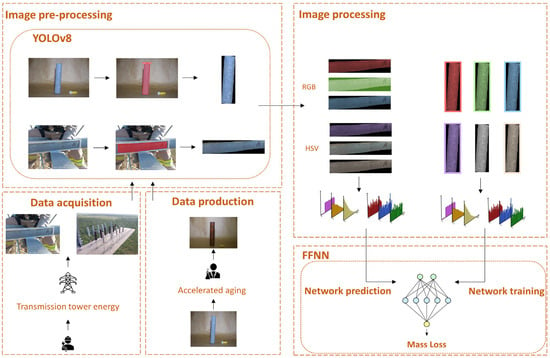
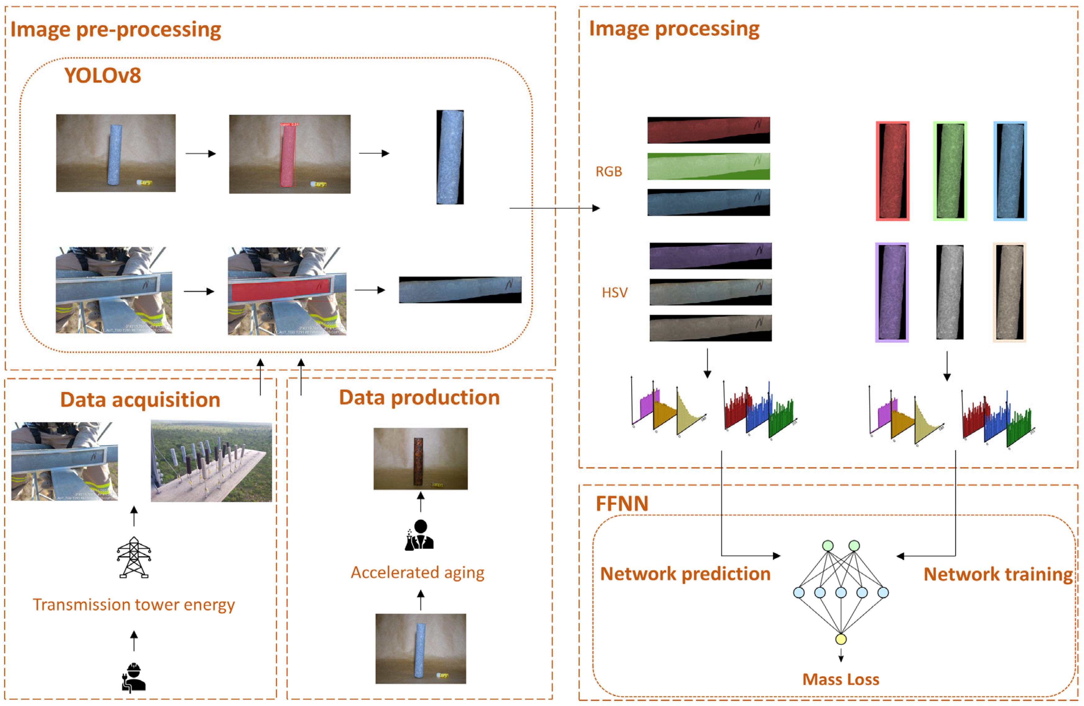
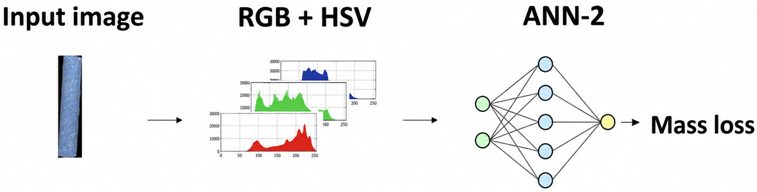
A methodology was developed to classify environmental corrosivity using visual data as input (images) and quantitative data as output (mass loss). The authors first assembled a dataset by photographing specimens and structural lattice components exposed to corrosion in the laboratory and in real-field settings. As the ANN-1, YOLOv8 [18] was applied to segment images and isolate corroded regions of interest (ROIs). From these ROIs, color histogram features were extracted in RGB and HSV color spaces, applying preprocessing such as color correction, normalization, or lighting compensation as needed. Finally, the ANN-2 was trained using these histogram features together with the measured mass loss per specimen (g) to predict the environmental corrosivity class or value. The flowchart of the process is shown in Figure 1.
Figure 1.
Flowchart of the ANN methodology. Data acquisition: illustration of the photographic locations of the trusses and coupons. Data production: Illustration of the accelerated aging process on coupons. Image pre-processing: Segmentation performed by ANN-1. Image processing: image separation performed by color spectra. FFNN: Trained model.
For the preparation of the database, the authors investigated and extracted numerical parameters from the images and their correlations with the observed mass losses. These numerical parameters were obtained from the characterization of the available images in color spectra, using both the RGB and the HSV color systems.
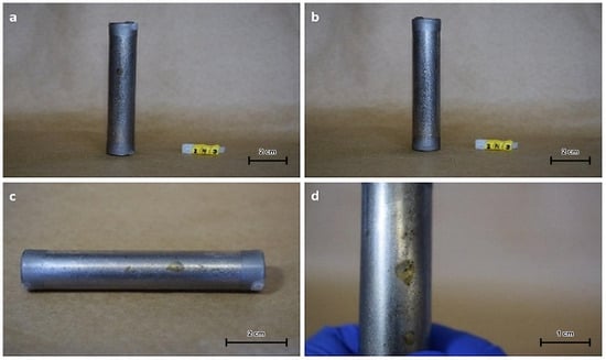
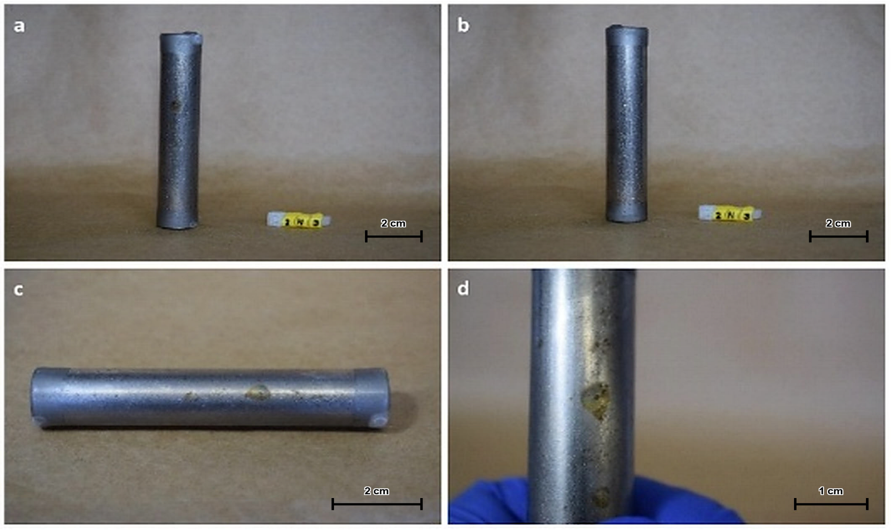
The methodology was applied to identify and quantify corrosion in AISI 1020 carbon steel via image segmentation. A dataset of 1798 images was assembled from test coupons exposed under both laboratory (artificial chambers) and field conditions. Corroded regions (Figure 2) were manually labeled, and the dataset was structured, formatted, and split into training, validation and test subsets in a 70:20:10 ratio. ANN-1 was trained to segment two distinct targets: the coupons, using this set, and the lattice structures of the transmission towers, using the 502 field images acquired at the georeferenced points and split in the same ratio. To ensure consistency, image acquisition followed a standardized protocol: coupon pretreatment, lighting, focal distance, camera resolution, and number of images per coupon were held constant, following established practices in the literature. ROIs corresponding to corroded areas were annotated on each coupon for use in training the network.
Figure 2.
Sample images illustrating the corrosion effect on specimen surfaces. (a) general view of the specimen surface; (b) general view of another specimen surface; (c) lateral view highlighting a localized corrosion region; (d) close-up view of the localized corrosion region.
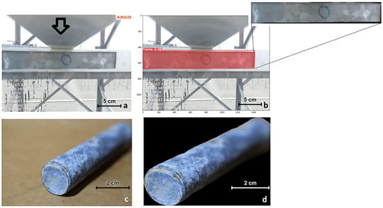
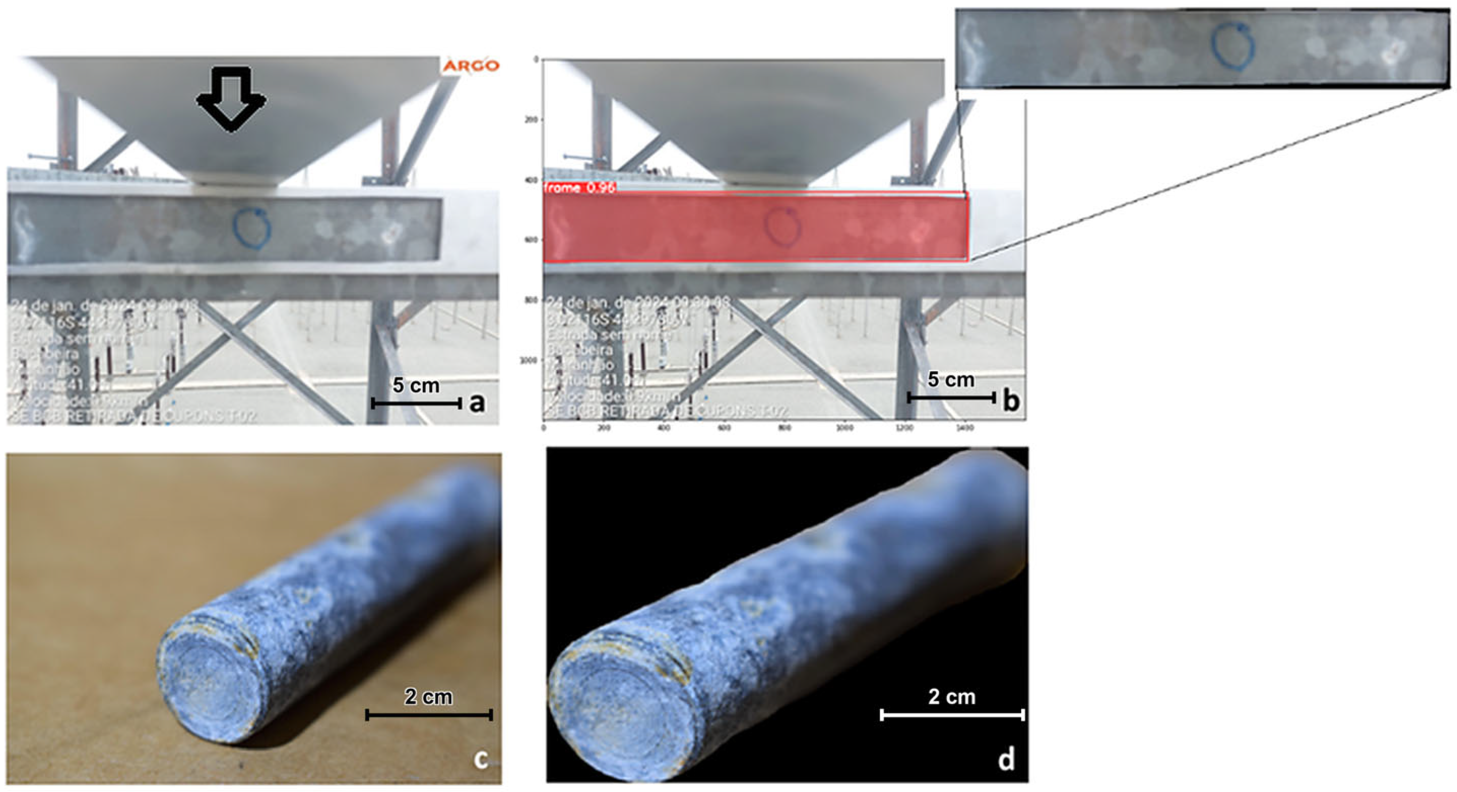
Subsequently, ANN-1 was trained to perform segmentation of the corroded regions. Figure 3 illustrates the result of the training and segmentation performance (Figure 3a,b), both for the truss of one of the inspected transmission towers and for one of the aged galvanized steel coupons (Figure 3c,d).
Figure 3.
Segmentation performance of the ANN-1, showing (a) the real image of one of the lattice structures photographed on a transmission tower (image extracted from the metal reference template installed on the tower); (b) the segmentation produced on that image; (c) the real image of one of the galvanized steel coupons; and (d) the corresponding segmentation obtained during training.
At each georeferenced location of the transmission towers (Table 1), 502 local images were taken of the metallic truss towers at positions facing north, south, east, and west. Coupons were collected at the same geographic positions. The focal distances were standardized, and the camera settings were kept constant throughout the entire seasonal analysis period. The data were comparatively analyzed using, for reference, the first image when the coupons were installed. Out-of-focus photos, images with the region of interest partially cut off, and those with shadowing were encountered, presenting a challenge for the network’s construction and validation.
To quantify this segmentation performance, ANN-1 was evaluated on the held-out validation subset of each dataset using standard instance-segmentation metrics: precision, recall, mAP50 (mean Average Precision at an IoU threshold of 0.5), and mAP50-95 (mean Average Precision averaged over IoU thresholds from 0.50 to 0.95). Because these metrics are computed by matching predicted and ground-truth masks across a range of IoU thresholds, mAP50-95 already incorporates and extends beyond a single averaged IoU value, and is reported here in its place. Results for both segmentation targets are summarized in Table 2.
Table 2.
Segmentation performance of ANN-1 on the held-out validation subset for both segmentation targets.
Both segmentation targets achieved high precision, recall, and mAP values, indicating that the regions of interest subsequently used to build the color histogram features for ANN-2 are reliably isolated from the surrounding image background. Representative examples of predicted segmentation masks against the corresponding ground-truth annotations, for both coupon and lattice validation images, are provided in Appendix B.
Using the Python 3.13.14 programming language, the corrosion rate images from AISI 1020 carbon steel were converted into RGB format. For each channel, the correlation between pixel intensity and the gravimetric mass loss measured on the corresponding coupon was examined across the full intensity range, and this correlation analysis guided the selection of the value ranges reported below. From the histograms of the reference images obtained in the accelerated tests, seven intervals of the RGB spectrum were delimited empirically as those that visually enhanced the distinction between corroded and intact regions. This step was conducted as an exploratory, heuristic analysis of chromatic sensitivity, with the aim of determining whether the color distribution contains information regarding the intensity of corrosion. The seven intervals reported here are illustrative examples of value ranges found to correlate with mass loss, rather than the result of an exhaustive search over all possible bound combinations. Similarly, neighboring bounds were also found to visually separate corroded from intact pixels, differing mainly in the degree of contrast achieved, which is consistent with the continuous nature of the underlying color response to corrosion rather than a sharp threshold effect. Three of these intervals partition the RED channel alone, which is consistent with the reddish-brown tones of the iron oxide corrosion products formed on carbon steel; the remaining four combine bounds on all three channels and were retained because they were also found to enhance the visual contrast of the corroded regions. These intervals are listed in Table 3. Because this exploratory stage does not feed into the final predictive model—ANN-2 is trained on complete color histograms rather than on these intervals, as described below—its results and, therefore, ANN-2’s performance do not depend on precisely how the seven intervals were delimited. The intervals reported in this subsection are the outcome of the preliminary exploratory stage and are presented here because they define the input representation subsequently evaluated for the FFNN, not as results of the predictive models.
Table 3.
Search intervals defined in the RGB spectrum for AISI 1020 carbon steel.
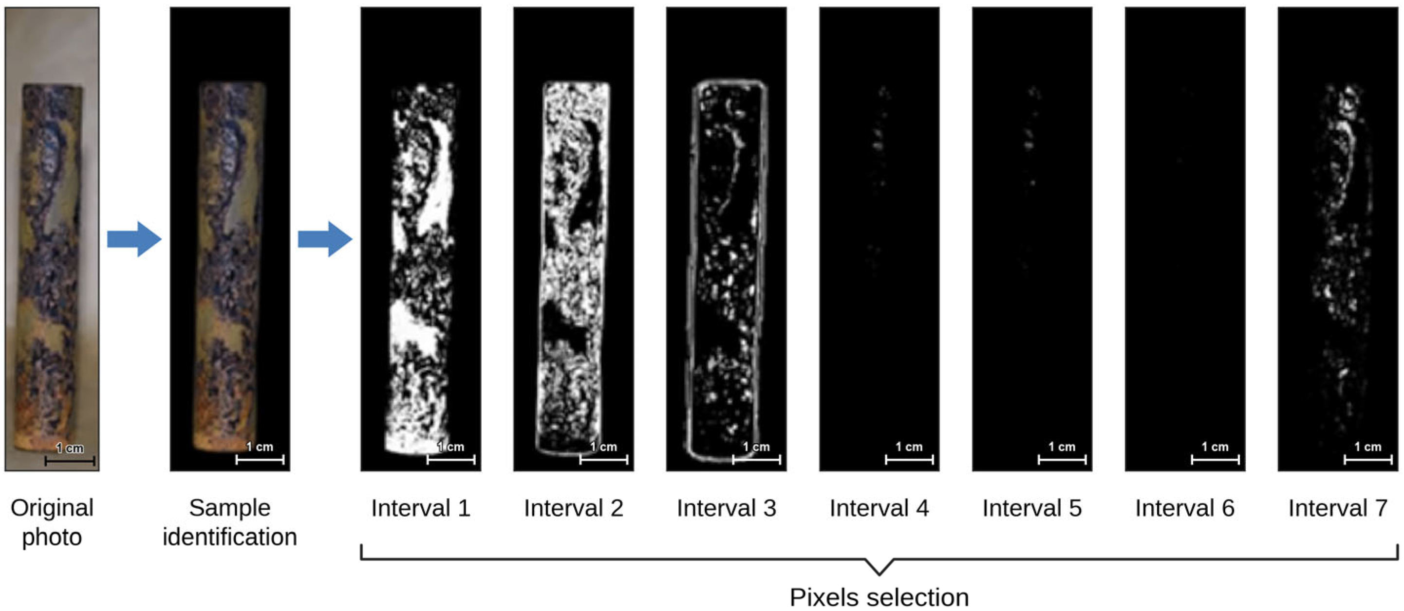
As an exploratory step, prior to the final ANN-2, the proportion of pixels falling within the delimited intervals was found to vary consistently with mass loss. The degree to which the corroded areas are highlighted depends on the interval selected, with some intervals isolating them clearly and others capturing few pixels of this material. The set of pixels selected by each interval on a carbon steel specimen is shown in Figure 4.
Figure 4.
Pixel selection for an AISI 1020 carbon steel specimen: original photograph, segmented sample identification, and the set of pixels selected by each of the seven RGB intervals listed in Table 3 (labeled 1 to 7).
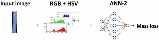
This approach supported the initial analysis of the relationship between selected color intervals and mass loss; however, the final ANN-2 model was trained using full color histograms extracted from the segmented regions, providing a more comprehensive representation of the image data, as illustrated in Figure 5.
Figure 5.
Flowchart for the development and testing of ANN-2, based on the process of transforming image data into equivalent mass loss.
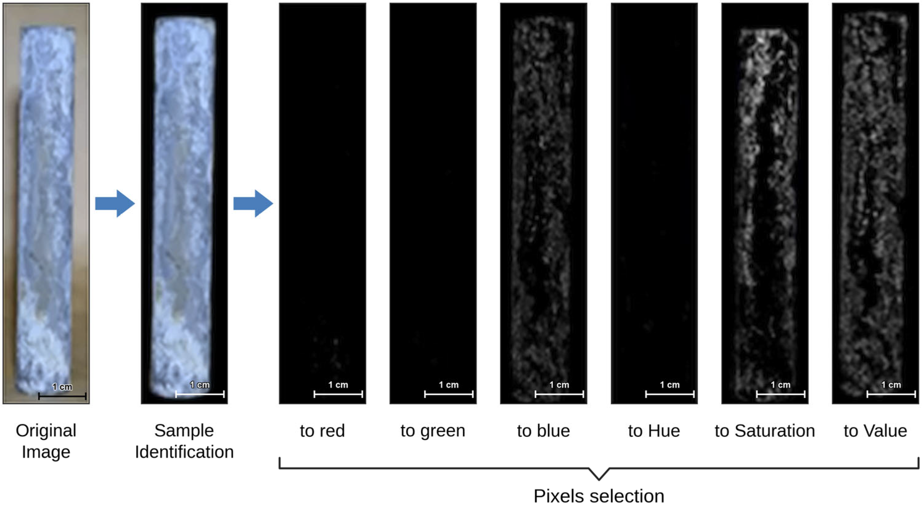
For galvanized steel, a similar procedure was developed. It was found that characterizing only the RGB spectrum would not allow effective analysis of representative pixels, due to the nature of the corrosion process in this material: the white corrosion products formed on the galvanized coating exhibit low chromatic contrast against the intact surface and are therefore poorly separable in RGB alone. Therefore, auxiliary search intervals in the HSV spectrum, specifically in the Saturation and Value channels, were incorporated alongside RGB, since these channels discriminate low-saturation, high-brightness regions more effectively. In addition, while for carbon steel, the RGB search intervals used in corrosion identification combined constraints for all channels at once, for galvanized steel, the intervals were defined considering each scoring level of the system as an independent variable. In other words, to count pixels associated with carbon steel corrosion, seven RGB intervals were used; for galvanized steel, six distinct intervals (one for each score) were established. The intervals adopted are shown in Table 4.
Table 4.
Search intervals defined in the RGB/HSV spectra for galvanized steel.
The ANN-1 architecture, YOLOv8-based, comprised 261 layers and 3,409,968 parameters. The training hyperparameters used were as follows: (1) epochs: 100; (2) batch size: 16; (3) image size: 640 pixels; (4) initial learning rate: 0.01; (5) beta1: 0.9; (6) beta2: 0.999; (7) epsilon: 1 × 10⁻⁸; (8) weight decay: 0.0005; (9) optimizer: Adam; and (10) mixed precision training.
The pixel count and its relationship to corrosion are shown in Figure 6.
Figure 6.
Pixel selection for a galvanized steel specimen: original photograph, segmented sample identification, and the set of pixels selected by each of the six RGB and HSV channel intervals listed in Table 4.
For the implementation of ANN-2, aimed at predicting the mass loss per specimen (g), the TensorFlow library [51] was utilized, enabling the architecture design capable of using nonlinearity through the activation functions and layers to find relations between the high-dimensional color histogram features and corrosion rates. The network comprises several layers (512, 512, 256, and 128 neurons) with the following configurations: activation function: ReLU for hidden layers and a linear activation for the output layer, dropout rate of 0.3 before the final dense layer to prevent overfitting, Adam optimizer with an initial learning rate of 0.001, β1 = 0.9, β2 = 0.999, ε = 1 × 10⁻⁷, evaluation metrics: Mean Absolute Error (MAE) and Mean Squared Error (MSE), number of epochs initially set to 2000, while early stopping was applied using a patience of 5 epochs, and batch sizes of 8 (AISI 1020 carbon steel) and 64 (galvanized steel). ANN-2 was trained on the histogram features extracted from the 1798 segmented coupon images, which are the specimens for which gravimetric mass loss was measured, divided into training, validation and test subsets in the same 70:20:10 ratio. In field application, the trained model is applied to the segmented lattice images, for which no gravimetric reference exists, so that mass loss is inferred from the relationship established on the coupons.
In the RGB space, each channel ranges from 0 to 255, representing natural colors. In the HSV space, the Hue channel ranges from 0 to 180, while the Saturation and Value channels range from 0 to 255. For each channel of each color space, a normalized histogram was computed, resulting in a total of 1461 input elements for the FFNN, which constitutes the complete feature representation used in the final model, in contrast to the reduced interval-based descriptors employed in the preliminary analysis.
To assess the ANN-2 training procedure stability, an additional sensitivity analysis was conducted by varying the batch size while iteratively excluding specific subsets from the training data. This complementary analysis was used to evaluate the robustness of the model to both mini-batch configuration and training-set composition; the result of this analysis led to the selection of final ANN-2 configurations. The complete results are presented in Appendix A, including Table A1 and Table A2 for galvanized steel and Table A3 and Table A4 for AISI 1020 carbon steel.
Also, ANN-3 was developed to use the parameters of the meteorological conditions recorded at the installation sites at the same location as the coupons and trusses in the power transmission towers. A FFNN was employed to predict the corrosion rate based exclusively on meteorological parameters recorded at the installation sites, without the use of image-derived features.
The FFNN configuration comprised four fully connected (FC) layers with 512, 512, 256, and 128 neurons. Additional configurations included a dropout rate of 40% for the last FC layer, ReLU as the activation function for every layer, and batch normalization after the first three layers. The training phase used the Adam optimizer with β1 = 0.9, β2 = 0.999, and ε = 1 × 10⁻⁷, 32 samples for batch size, Glorot weight initialization and early stopping of 5 epochs. The output data from this network comprised the atmospheric corrosion classes based on the resulting mass losses, ranging from C3 to Cx. The meteorological dataset comprised hourly records collected over one year of exposure by one weather station installed at each collection point, that is, one station per tower and one per substation, divided into training, validation and test subsets in the same 70:20:10 ratio.
Finally, to support the analysis of corrosivity prediction in transmission towers, an intuitive interface was designed to facilitate geospatial and temporal visualization of data. Corrosion results were correlated with the meteorological conditions obtained, enabling detailed analysis of regions with higher corrosion risk and, consequently, decision-making about the feasibility of installing new transmission towers in those areas.
3. Results and Discussion
Based on the investigation and extraction of numerical parameters from images of AISI 1020 carbon steel coupons exposed in an artificial weathering chamber (salt spray) in the RGB and HSV color spaces, initial analyses using predefined color intervals were performed to verify the correlation between visual patterns and corrosion rates; subsequently, the final model was trained using full color histograms to capture a more comprehensive representation of the image data. These values were used to build the training dataset for the ANN-2 to reproduce the pattern between the pixels’ color and specific levels of corrosion. The mass loss results are shown partially in Table 5. Overall, the methodology was found to have potential for corrosion quantification, with experimental mean values of (1184 ± 226) µm·year−1 and neural network predictions of (1204 ± 202) µm·year−1, expressed as the thickness-loss rate obtained from the gravimetric mass loss by Equation (1), as adopted for all accelerated-chamber results (Section 2.1).
Table 5.
Neural network training results for corrosion rate prediction of AISI 1020 carbon steel exposed in a salt spray chamber. Values are thickness-loss rates in µm·year−1, obtained from the gravimetric mass loss by Equation (1).
Similarly, the results after ANN-2 training are presented for the corrosion rate (in µm·year−1) of galvanized steel exposed in a salt spray chamber in Table 6. The proposed methodology proved substantially effective in quantifying mass loss based on image color spectra, with the experimental corrosion rate being (63 ± 49) µm·year−1, compared to the ANN-predicted value of (61 ± 44) µm·year−1.
Table 6.
Neural network training results for the corrosion rate of galvanized steel exposed in a salt spray chamber. Values are thickness-loss rates in µm·year−1, obtained from the gravimetric mass loss by Equation (1).
The metrics used for evaluation were the MAE and the coefficient of determination (R2). Because ANN-2 regresses the gravimetric mass loss, the MAE is reported in grams per specimen, the unit in which the network operates; the corrosion rates in Table 5 and Table 6 are the same quantity after conversion using Equation (1). The results are shown in Table 7.
Table 7.
Statistical performance metrics of ANN-2 for mass loss prediction on the held-out test subset of the field dataset for the final configuration adopted. MAE is expressed as mass loss per specimen, in g.
Both cases showed good predictive performance, as indicated by the R2 scores. Direct comparison with alternative models is limited for two reasons. First, no public benchmark dataset pairs corrosion images with gravimetric mass-loss measurements, so no external reference is available. Second, most existing approaches address corrosion detection or corroded-area estimation, tasks whose metrics are not commensurable with the direct prediction of mass loss pursued here. The present methodology targets the direct prediction of mass loss from image-derived features, which remains less explored in the literature. AISI 1020 carbon steel exhibited better prediction, likely because the visual appearance of the coupons makes it easier to distinguish between corroded and non-corroded areas. On the other hand, for galvanized steel, the corrosion does not produce such a clearly distinguishable contrast between those areas, which is reflected in a lower R2. Nevertheless, both materials exhibited small MAE values. A paired significance test comparing predicted and measured mass loss for both materials is reported in Appendix A.3, confirming no statistically significant difference at the 5% level.
Because the dataset comprises repeated acquisitions of the same specimens and multiple orientations of the same towers, a random split would allow images of a given site to appear in both the training and the test sets. To rule out this effect, ANN-2 was retrained excluding one entire site from the training set at a time, so that the held-out site was never seen during training. The full results are reported in Appendix A. Performance remained within the same range across all held-out sites, which indicates that the model generalizes to locations it has not observed rather than exploiting site-specific redundancy in the data.
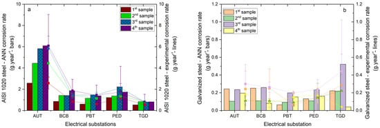
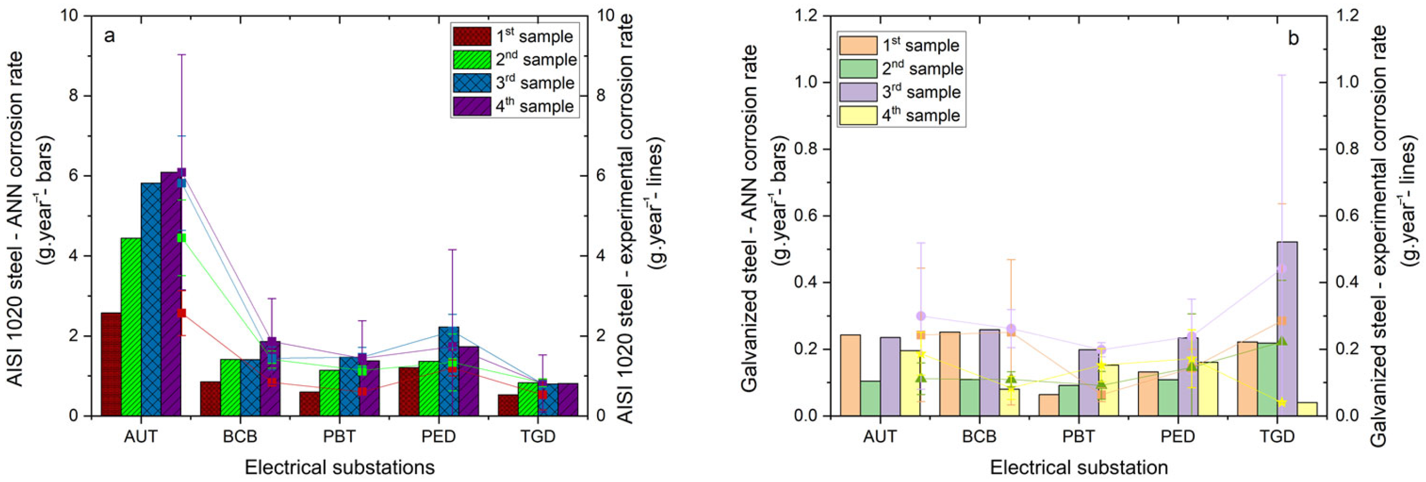
After training the ANN with the coupons exposed in artificial weathering chambers, the methodology was applied to predict the corrosion rate of AISI 1020 carbon steel and galvanized steel samples exposed for one year at the substations AUT, BCB, PBT, PED, and TGD (Northeast Brazil). The results are shown in Figure 7a for AISI 1020 carbon steel and Figure 7b for galvanized steel.
Figure 7.
Graphs of mass loss of AISI 1020 carbon steel and galvanized steel coupons in g·year−1 per specimen, accumulated over one year of exposure and obtained from the fourth quarterly retrieval, at electrical substations in northeastern Brazil (Tianguá, TGD; Bacabeira, BCB; Parnaíba, PBT; Acaraú, AUT; and Pecém, PED): (a) AISI 1020 carbon steel (bars: ANN-predicted values, and lines: experimental data), and (b) galvanized steel (bars: ANN-predicted values, and lines: experimental data).
The mean values predicted for AISI 1020 carbon steel by the ANN fell within the obtained error margins. Consistent with Section 2.1, field results are given as the mass loss per specimen accumulated over one year of exposure, in g·year−1; the thickness-loss rates on which the ISO 9223 classification reported below is based were obtained from these values through Equation (1). The values obtained were as follows: (a) AUT, experimental (Exp) = (4.73 ± 1.61) g·year−1, ANN = (4.74 ± 1.60) g·year−1; (b) BCB, Exp = (1.39 ± 0.42) g·year−1, ANN = (1.38 ± 0.43) g·year−1; (c) PBT, Exp = (1.16 ± 0.40) g·year−1, ANN = (1.18 ± 0.42) g·year−1; (d) PED, Exp = (1.60 ± 0.41) g·year−1, ANN = (1.62 ± 0.48) g·year−1; and (e) TGD, Exp = (0.74 ± 0.14) g·year−1, ANN = (0.76 ± 0.12) g·year−1.
For AISI 1020 carbon steel, the environmental aggressiveness predicted by the ANN at the electrical substations was AUT (C5) > PED (C4) > BCB (C4) > PBT (C3) > TGD (C3), which was consistent with the experimental mass-loss measurements. The category reported for each site is the one most frequently obtained among its four monitoring points, each classified individually from its own triplicate coupons; it is therefore not recoverable by applying Equation (1) to the site mean alone, which for BCB and PED falls close to the C3/C4 boundary.
For galvanized steel, the aggressiveness sequence, from highest to lowest, was as follows (Exp): TGD (0.25 ± 0.17) g·year−1 (C5-Cx) > AUT (0.21 ± 0.08) g·year−1 (C5) > BCB (0.18 ± 0.09) g·year−1 (C5) = PBT (0.18 ± 0.05) g·year−1 (C5) > PED (0.13 ± 0.06) g·year−1 (C5).
The ANN-predicted data followed nearly the same sequence of environmental aggressiveness observed experimentally, with a slight deviation for PBT, which presented a lower mean value: TGD (0.25 ± 0.20) g·year−1 (C5–Cx) > AUT (0.19 ± 0.06) g·year−1 (C5) > BCB (0.18 ± 0.09) g·year−1 (C5) > PED (0.17 ± 0.05) g·year−1 (C5) > PBT (0.13 ± 0.06) g·year−1 (C5).
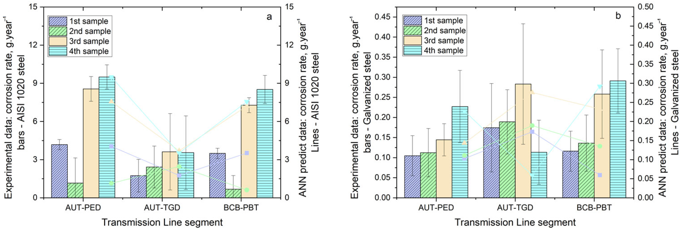
The same procedure was applied to the field samples located on the georeferenced power transmission towers, and the graphical results are shown in Figure 8a for the coupons of AISI 1020 carbon steel and Figure 8b for the galvanized steel coupons. The average values predicted by the ANN were within the mean and standard deviations of the experimental data (Exp), both for AISI 1020 carbon steel and for galvanized steel. For the AUT-PED section and AISI 1020 carbon steel: (i) Exp = (5.85 ± 3.89) g·year−1, ANN = (4.25 ± 3.21) g·year−1; (ii) AUT-TGD, Exp = (2.83 ± 0.91) g·year−1, ANN = (2.64 ± 0.98) g·year−1; and (iii) BCB-PBT, Exp = (4.99 ± 3.58) g·year−1, ANN = (3.78 ± 3.30) g·year−1. In both the experimental and predicted measurements, the TL segments, in terms of environmental aggressiveness, were classified for AISI 1020 carbon steel as AUT-PED (C5–Cx) > BCB-PBT (C5–Cx) > AUT-TGD (C5).
Figure 8.
Graphs of mass loss of AISI 1020 carbon steel and galvanized steel coupons g·year−1 per specimen, accumulated over one year of exposure and obtained from the fourth quarterly retrieval at transmission line segments in northeastern Brazil (AUT-PED, AUT-TGD, and BCB-PBT): (a) AISI 1020 carbon steel (bars: experimental data, and lines: ANN-predicted values), and (b) galvanized steel (bars: experimental data, and lines: ANN-predicted values).
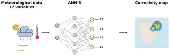
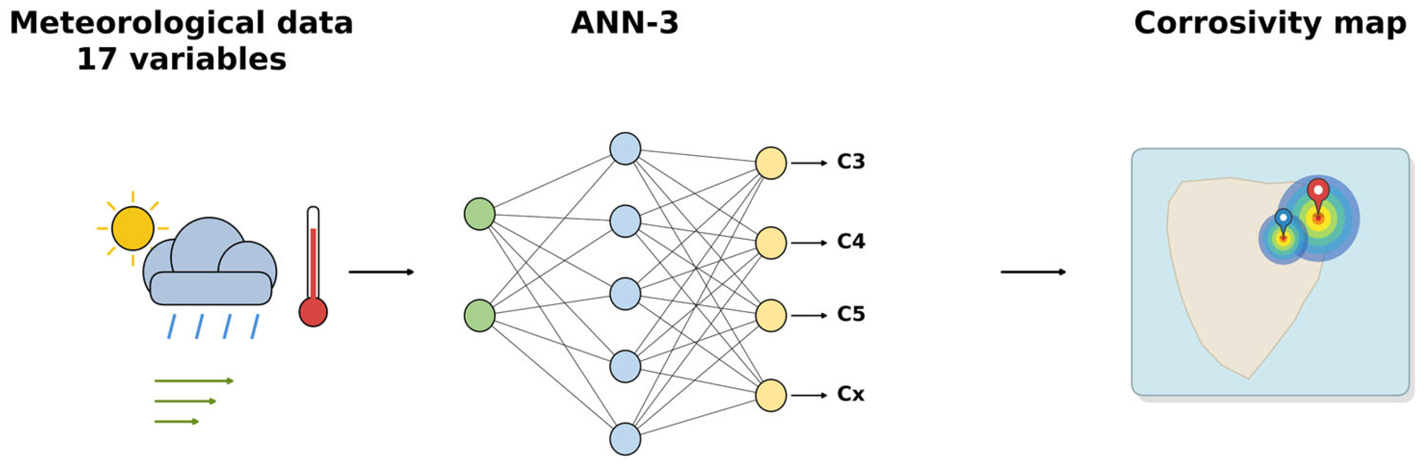
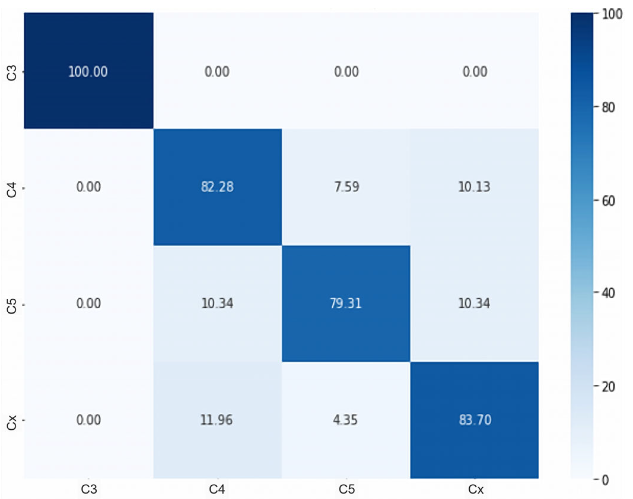
In addition to the image-based mass-loss prediction performed by ANN-2, the classification performance of ANN-3 was evaluated using only meteorological parameters recorded at the installation sites. Figure 9 summarizes the ANN-3 pipeline: the seventeen meteorological input variables are processed by the network to yield the predicted atmospheric corrosivity class, with the results summarized in the confusion matrix shown in Figure 10.
Figure 9.
Schematic overview of the ANN-3 pipeline: seventeen meteorological variables recorded at each installation site are used as input to a feedforward neural network, which classifies the site into an atmospheric corrosivity class (C3, C4, C5, or Cx).
Figure 10.
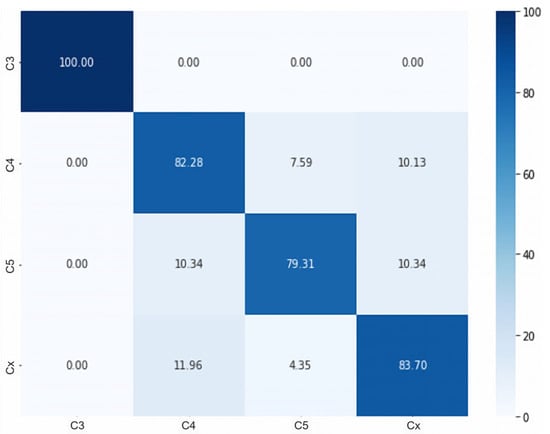
Confusion matrix for ANN-3 in the classification of atmospheric corrosivity classes.
ANN-3 reached an overall classification accuracy of 85%, and the confusion matrix indicates a high agreement for the individual atmospheric corrosivity classes. Class C3 was correctly identified in all evaluated cases, while C4, C5, and Cx also showed high percentages of correct classification. Most misclassifications occurred between adjacent classes, particularly between C4 and C5, and between C5 and Cx. This pattern is the one expected for an ordinal target: the ISO 9223 categories are contiguous intervals of a continuous corrosion rate, so specimens near a category boundary may fall on either side without the prediction being physically wrong. A smaller number of cases spanned more than one category; these represent the conditions under which the meteorological variables alone are least discriminating, and they delimit the applicability of an environment-based classification when image-derived information is not used. A permutation feature importance analysis of the seventeen meteorological inputs, together with a comparison against a reduced five-variable model trained on only the top-ranked variables, is reported in Appendix D, confirming that the full input set carries information beyond the top-ranked variables, particularly for resolving the harder C4/C5/Cx boundary.
To complement the confusion matrix, Table 8 reports per-class precision, recall, and F1-score for ANN-3, with macro-averaged values of 86.49%, 86.32%, and 86.34%, respectively.
Table 8.
Per-class precision, recall, and F1-score for ANN-3.
As a baseline comparison, a multinomial logistic regression classifier was trained on the same 17 standardized meteorological input variables, using the lbfgs solver with default L2 regularization (C = 1.0) and a maximum of 2000 iterations, under the identical class-balanced sampling and train/validation/test protocol described in Section 2.3. The baseline reached 67.15% overall accuracy on its held-out test subset, substantially below the 85% accuracy achieved by ANN-3 (Figure 10)—a gap of nearly 18 percentage points. Per-class precision, recall and F1-score for the baseline are reported in Table 9, indicating that ANN-3 captures non-linear, class-discriminative structure in the meteorological variables that a linear model cannot.
Table 9.
Logistic regression baseline performance per class.
The raw dataset used to train ANN-3 is markedly imbalanced across corrosivity classes: of 5049 labeled records, 2737 (54%) belong to class C5, 1156 (23%) to C3, and 578 (11%) each to C4 and Cx. This imbalance mirrors the environmental conditions actually measured at the monitored sites, rather than a sampling design choice: the corrosivity class of a given site and retrieval period is itself derived from the gravimetric mass-loss measurements described in Section 2.1 and therefore only becomes known once that measurement is complete. Because the eventual class distribution cannot be anticipated during the design of the monitoring campaign, monitoring effort could not have been allocated in advance to balance it. To prevent this imbalance from biasing training toward the majority class, each class was undersampled to the minority-class count (578 records) prior to the train/validation/test split so that the reported metrics reflect balanced-class performance rather than being inflated by the natural prevalence of C5.
Based on field-collected corrosion and meteorological data, a graphical interface was developed to provide a rapid visual assessment of local environmental corrosivity, supporting decisions on maintenance, material selection, and surface treatments for new or existing installations. The interface combines a georeferenced heatmap, a bar chart of corrosion rates, and a timeline of meteorological parameters, implemented with Python libraries; further details and screenshots are provided in Appendix C.
4. Conclusions
In this study, visual patterns in digital images (RGB and HSV color spaces) were correlated with corrosion rates using ANNs for steels exposed in salt spray chambers and in the field. It is concluded that in the exploratory identification, some pixel ranges have high correlation to mass loss, enabling the construction of robust prediction models. In the accelerated chamber tests, with corrosion expressed as the thickness-loss rate, the ANN estimates closely matched the experimental measurements for AISI 1020 carbon steel (1204 ± 202 vs. 1184 ± 226 µm·year−1) and for galvanized steel (61 ± 44 vs. 63 ± 49 µm·year−1), with low MAE and high R2.
Applying the model to real samples from substations in Northeast Brazil yielded predictions within the experimental error margins, accurately reproducing the order of environmental aggressiveness among locations. At the most aggressive substation, the ANN predicted 4.74 ± 1.60 g·year−1 per specimen against 4.73 ± 1.61 g·year−1 measured, and at the least aggressive, 0.76 ± 0.12 g·year−1 against 0.74 ± 0.14 g·year−1—field values being reported per specimen throughout, as defined in Section 2.1—reproducing the experimental ranking AUT > PED > BCB > PBT > TGD. ANN-3, using meteorological variables alone, assigned the corrosivity category correctly in 85% of cases, with the residual disagreement largely confined to adjacent categories. For the galvanized steel, a slight deviation in ranking between two sites was observed, suggesting a lower visual contrast between corroded and non-corroded areas.
In the georeferenced transmission towers, the ANN’s predictions also stayed within experimental uncertainties, confirming the aggressiveness classification as AUT-PED > BCB-PBT > AUT-TGD.
The developed graphical interface, which may be adaptable to other studies and locations, enables practical visualization of local environmental corrosivity (through maps, bar charts, and temporal series), supporting decisions regarding maintenance, material selection, or surface treatments. For the transmission operator, the practical consequence is the possibility of replacing calendar-based inspection of remote lattice structures with a risk-ranked schedule derived from locally measured corrosivity, concentrating recoating budgets on the spans where the residual coating life is shortest and thereby reducing the exposure of the transmission link to corrosion-induced unavailability. Because this corrosivity estimate can be obtained from a single inspection photograph rather than the standardized one-year gravimetric exposure required by ISO 9223/9226, the maintenance schedule can be kept dynamic, continuously refocused on the spans that most urgently require attention rather than fixed to a static calendar.
4.1. Limitations
Despite the performance obtained, this study has limitations that should be acknowledged. The first limitation is intrinsic to the design: ANN-2 is calibrated on coupons, for which gravimetric mass loss can be measured, and is then applied to lattice images, for which no gravimetric reference exists. This is a domain transfer, and its validity rests on the assumption that the color signature of the corrosion products is comparable on the two surfaces. This domain transfer is further supported by three aspects of the experimental design. First, the coupons and the metal reference template are exposed to the same atmospheric conditions: both are installed at the same site and at equivalent heights on the tower (Section 2.1), so the two surfaces experience, in principle, an equivalent corrosive environment and comparable degradation over time. Second, ANN-1 segments both coupon and lattice reference-template images into the same rectangular region-of-interest format prior to color-histogram extraction, so ANN-2 receives an input representation that is structurally identical regardless of the source; the lattice images used are photographs of this metal reference template installed on the tower, made of the same material and cross-section as the retrieved coupons (Figure 3), rather than of the structural lattice steel itself, so the two image sets share the same underlying material and surface geometry, differing mainly in whether the specimen was later removed for gravimetric weighing. Third, because ANN-2 operates on normalized color histograms rather than on raw pixel arrays, its input representation is inherently invariant to the object’s shape or surrounding context and depends only on the color distribution of the photographed material surface—a property that would hold regardless of the segmentation geometry. The held-out-site experiments reported in Appendix A, in which each site was excluded from training in turn, were designed to probe this assumption; performance remained within the same range across all held-out sites, but a direct gravimetric validation on lattice material was not possible within the scope of this study. To probe the temporal stability of this domain transfer, ANN-2 was additionally applied separately to each of the four quarterly field retrievals; the resulting prediction error did not increase across retrievals, providing no evidence of drift over the one-year monitoring period (Appendix A.2). The dataset was assembled from a specific geographic region, which may affect the model’s generalizability to other climatic zones or atmospheric environments. Additionally, none of the monitored sites registered corrosivity below class C3 during the study period, so the proposed methodology has not been validated for very low corrosivity environments (classes C1 and C2). The methodology relies on image quality, and variations in lighting conditions, camera angle, or surface preparation may introduce uncertainty in the predictions. Field images were collected only under suitable weather conditions (i.e., without rain or heavy overcast), which constrains the range of lighting variability actually present in the dataset relative to an unconstrained field-acquisition protocol. Furthermore, all coupons and reference templates were installed at a fixed height of 20 m on both towers and substations; extending the experimental campaign to multiple heights per site, in addition to the 40 monitoring points already covered over 1150 km and one year of quarterly retrievals, was not feasible within the scope of this study, so the dataset does not capture the height-dependence of corrosion rate reported elsewhere in the literature.
4.2. Future Work
However, the proposed methodology is designed to be transferable across different environments, as it captures fundamental corrosion patterns through image features and environmental variables, and future work could extend it to other climatic zones and global datasets. Quantifying, in isolation, the effect of lighting variability on prediction uncertainty was outside the scope of the present study and remains an open point for future investigation. Furthermore, the current models are based on FFNN architectures; future work could explore different models, potentially improving predictive performance. Expanding the dataset to include other metals, coatings, and exposure conditions would also broaden the applicability of the approach. Because the current meteorological inputs do not include direct measurements of airborne chloride or pollutant deposition—a key driver of coastal corrosivity—a promising direction for future work is the development of an analogously rapid, non-destructive methodology for estimating airborne chloride and pollutant concentration, which, combined with the present image-based framework, would yield a more complete fast-assessment approach to atmospheric corrosivity. With these advances, the proposed methodology could become an efficient and effective tool for corrosion monitoring and prediction in real-world infrastructure applications.
Author Contributions
Conceptualization, L.L., B.C.K., A.L. and F.A.D.; methodology, L.L., M.D.G.P.B., J.S.C.A. and B.C.K.; software, L.L. and B.C.K.; validation, C.M.G.P., M.D.G.P.B., J.S.C.A. and K.F.P.; formal analysis, L.L. and K.F.P.; investigation, L.L., C.M.G.P., M.D.G.P.B., J.S.C.A. and B.C.K.; resources, C.M.G.P.; data curation, L.L., C.M.G.P., M.D.G.P.B., J.S.C.A. and K.F.P.; writing—original draft preparation, L.L.; writing—review and editing, C.M.G.P. and K.F.P.; visualization, L.L., A.L. and F.A.D.; supervision, K.F.P., A.L. and F.A.D.; project administration, A.L. and F.A.D. All authors have read and agreed to the published version of the manuscript.
Funding
This research was funded by ARGO ENERGIA and ANEEL, R&D project 010737-0002_2022.
Data Availability Statement
The datasets presented in this article are not readily available because of contractual restrictions. Requests to access the datasets should be directed to the corresponding author.
Acknowledgments
The authors would like to acknowledge the support in financial resources and infrastructure by the companies ARGO ENERGIA, ANEEL and Lactec, R&D project 010737-0002_2022.
Conflicts of Interest
Alexandre Latorre and Fernando Almeida Diniz were employed by the ARGO Energia. The remaining authors declare that the research was conducted in the absence of any commercial or financial relationships that could be construed as a potential conflict of interest. The authors declare that this study received funding from the companies ARGO ENERGIA, ANEEL and Lactec. The funder was not involved in the study design, collection, analysis, interpretation of data, the writing of this article or the decision to submit it for publication.
Abbreviations
The following abbreviations are used in this manuscript:
| ABNT | Associação Brasileira de Normas Técnicas |
| AISI | American Iron and Steel Institute |
| ANN | Artificial Neural Network |
| CNN | Convolutional Neural Network |
| DFP | Differential Flower Pollination |
| ES | Energy Substation |
| FFNN | Feedforward Neural Network |
| GA | Genetic Algorithm |
| GS-SVM | Grid Search Support Vector Machine |
| HSV | Hue, Saturation, Value |
| IoU | Intersection over Union |
| ISO | International Organization for Standardization |
| LSHADE | History-based Adaptive Differential Evolution with Linear Population Size Reduction |
| MAE | Mean Absolute Error |
| mAP | Mean Average Precision |
| MLP | Multi-Layered Perceptron |
| MSE | Mean Squared Error |
| NBR | Norma Brasileira |
| PSO-SVM | Particle Swarm Optimization Support Vector Machine |
| RGB | Red, Green, Blue |
| RNN | Recurrent Neural Network |
| ROI | Region of Interest |
| SVM | Support Vector Machine |
| TL | Transmission Line |
| YOLO | You Only Look Once |
Appendix A
Appendix A.1. Sensitivity Analysis of ANN-2
To evaluate the ANN-2 robustness against site-specific overfitting and to select the final configuration adopted in the main manuscript, a sensitivity analysis was performed by varying the batch size and iteratively excluding specific subsets (TL or ES) from the training dataset. In each experiment, the subset identified in the corresponding row was removed from the training set, and the network was trained using the remaining data. The reported metrics therefore reflect the predictive behavior of the model under controlled variations in both mini-batch configuration and training-set composition.
Table A1 and Table A2 present the results for galvanized steel in terms of MAE and MSE, respectively. Similarly, Table A3 and Table A4 present the results for AISI 1020 carbon steel in terms of MAE and MSE, respectively. In all four tables, the error metrics refer to the mass loss per specimen, so that MAE is expressed in g and MSE in g2, and each cell reports the error followed by the corresponding R2.
Table A1.
Performance of ANN-2 for galvanized steel under MAE loss, different batch sizes, and held-out subset conditions.
Table A2.
Performance of ANN-2 for galvanized steel under MSE loss, different batch sizes, and held-out subset conditions.
Table A3.
Performance of ANN-2 for AISI 1020 carbon steel under MAE loss, different batch sizes, and held-out subset conditions.
Table A4.
Performance of ANN-2 for AISI 1020 carbon steel under MSE loss, different batch sizes, and held-out subset conditions.
Overall, this analysis verified whether the proposed ANN-2 remained stable when relevant portions of the dataset were withheld during training and batch size changes, although some variation was observed depending on the adopted configuration. This behavior is expected given the heterogeneity of the dataset and suggests that the final model is influenced not only by the mini-batch configuration but also by the representativeness of the training data. Even so, the general predictive behavior remains consistent, supporting the robustness of the final training strategy adopted in the main study.
Appendix A.2. Temporal Stability of ANN-2 Predictions on Field Images
To assess whether ANN-2’s predictions drift over the course of the one-year field monitoring period, the trained model was applied independently to the lattice reference-template images from each of the four quarterly retrievals, and the resulting predictions were compared against the gravimetric mass loss measured on galvanized steel coupons from the same towers and retrieval periods, aggregated at the transmission-line-segment level. The mean absolute error per retrieval is reported in Table A5.
Table A5.
Mean absolute error of ANN-2 predictions (galvanized steel) per quarterly field retrieval, aggregated at the transmission-line-segment level.
The error does not increase monotonically across retrievals, indicating no evidence of systematic drift in ANN-2’s predictions over the monitoring period; the retrieval-to-retrieval variation observed is consistent with the sampling noise already characterized in Appendix A.1.
Appendix A.3. Statistical Significance of ANN-2 Predictions
To formally test whether the model’s predictions differ from the gravimetric measurements, a paired t-test and a Wilcoxon signed-rank test were applied to the held-out test-set values of predicted and measured mass loss, separately for AISI 1020 carbon steel and galvanized steel. Table A6 reports the results.
Table A6.
Paired significance tests for ANN-2 predictions on the held-out test set.
For both materials, neither test indicates a statistically significant difference between predicted and measured mass loss at α = 0.05, providing additional statistical support for the validity of ANN-2’s predictions beyond the MAE and R2 reported in Section 3.
Appendix B
Segmentation Performance of ANN-1
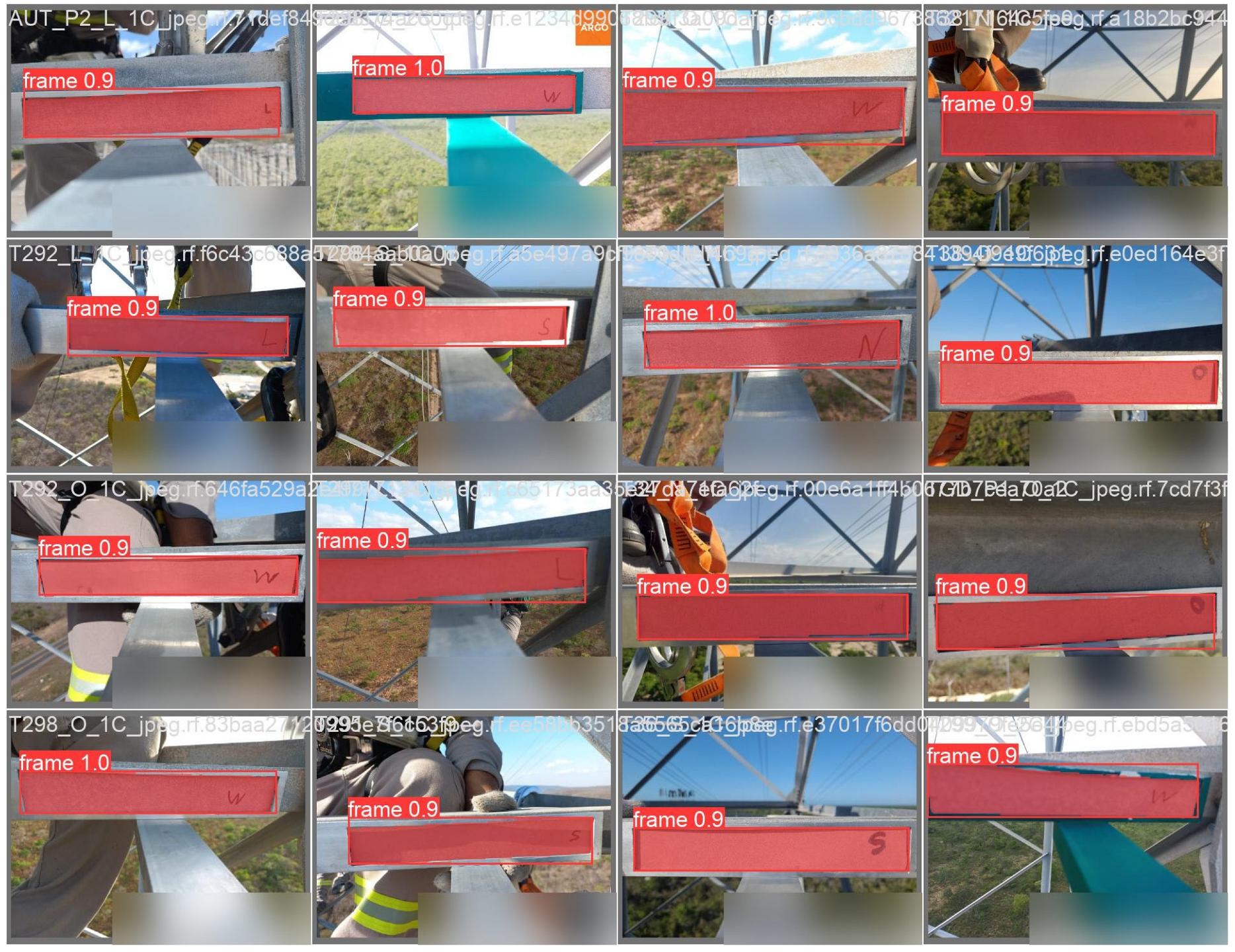
Figure A1 and Figure A2 shows representative predicted segmentation masks obtained by ANN-1 on the held-out validation subset (red overlay, with the associated confidence score), compared against the corresponding ground-truth region of interest, for both segmentation targets described in Section 2.3 and quantified in Table 2.
Figure A1.
Representative predicted segmentation masks (red overlay, with confidence score) obtained by ANN-1 on the held-out validation subset, compared against the ground-truth region of interest for AISI 1020 carbon steel and galvanized steel coupons.
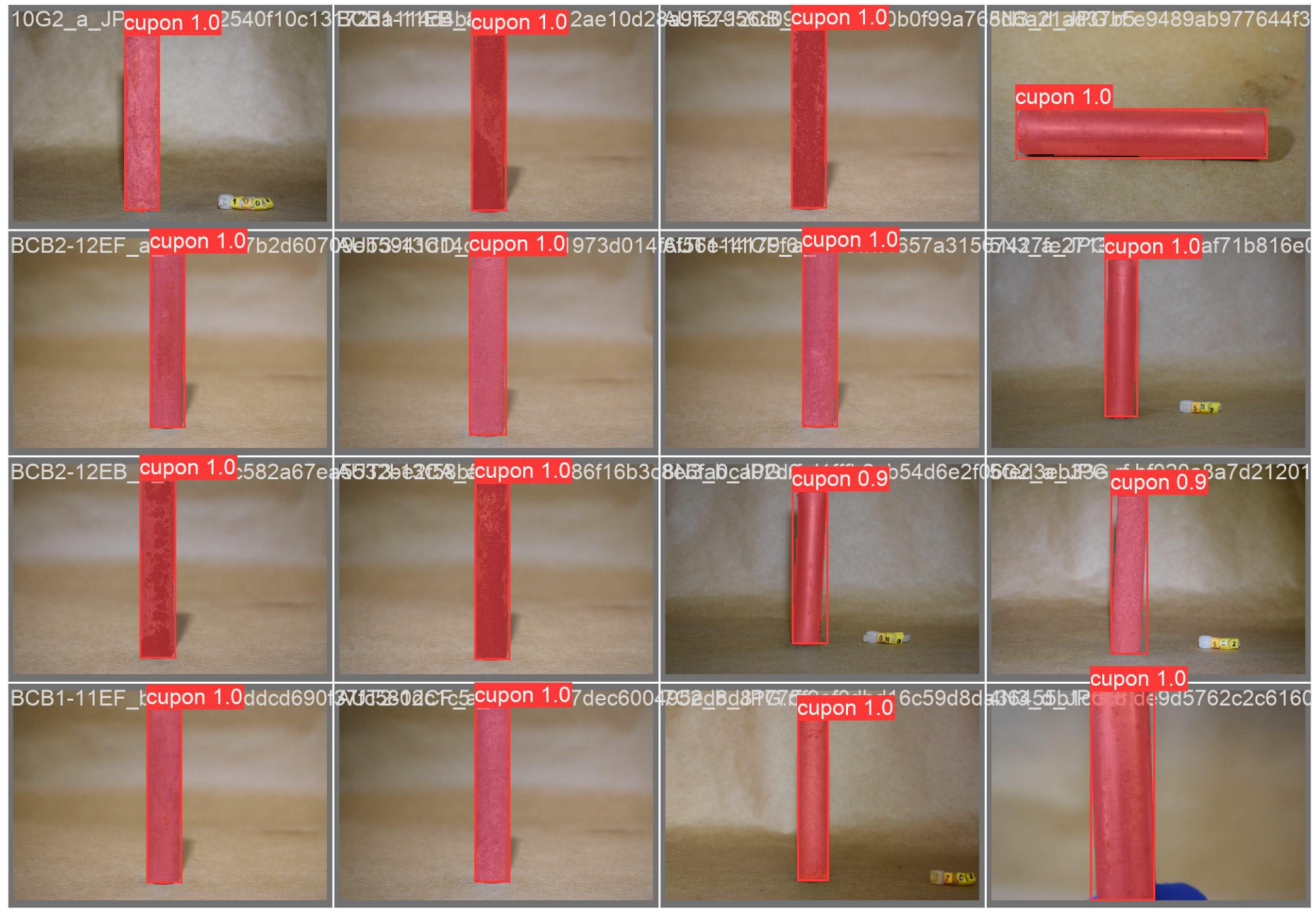
Figure A2.
Representative predicted segmentation masks (red overlay, with confidence score) obtained by ANN-1 on the held-out validation subset, compared against the ground-truth region of interest for lattice structure reference frames on transmission towers.
Appendix C
Graphical Interface for Corrosivity Visualization
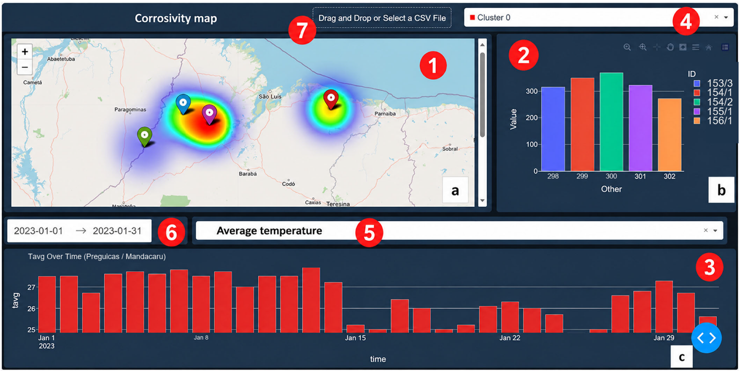
Figure A3 shows the components of the interface introduced in Section 3. The interactive map, located at the center of the interface, serves as the primary tool. Using the Folium library, this map generates a heatmap that visually represents the spatial distribution of corrosivity; areas with high corrosion intensity are highlighted in warm colors such as red and orange, while regions with lower corrosivity are depicted in cool colors such as blue and green, facilitating the rapid identification of critical zones that may require more frequent maintenance or could influence decisions regarding the establishment of new towers in the area. Positioned to the right of the map, the bar chart (Figure A3b) was developed using the Plotly 6.9.0 library; it complements the geographic visualization by providing a graphical representation of corrosion rate data over the selected period, enabling the observation of variations among data points within the grouped region—a feature particularly valuable for identifying patterns that may be influenced by environmental factors such as humidity, temperature, and precipitation. At the bottom of the interface, the timeline chart (Figure A3c) provides a detailed view of meteorological parameters, such as average temperature over time, allowing users to directly correlate meteorological conditions with observed corrosion rates.
Figure A3.
Components of the corrosivity rate interface, comprising: (a) the georeferenced heatmap generated using the Folium library; (b) the bar chart developed using the Plotly library; and (c) the timeline chart for meteorological parameters. The numbered interface components correspond to: (1) georeferenced corrosivity heatmap; (2) bar chart displaying the selected cluster data; (3) timeline chart of the selected meteorological parameter; (4) cluster selection menu; (5) meteorological parameter selection menu; (6) date-range selector; and (7) CSV file upload area.
Appendix D
Appendix D.1. Permutation Feature Importance
To assess which meteorological variables most influence ANN-3’s classification, permutation feature importance was computed on the held-out test set (n = 347): each of the seventeen input variables was independently shuffled (30 repetitions), and the resulting drop in classification accuracy was recorded. Table A7 presents the ranked results.
Table A7.
Permutation feature importance of ANN-3’s meteorological inputs.
The five most influential variables were gust speed, mean temperature, and mean, maximum, and minimum humidity, together accounting for most of the model’s discriminative signal, while wind-speed extremes and maximum atmospheric pressure contributed negligibly.
Appendix D.2. Reduced-Feature Model Comparison
To test whether a smaller input set could achieve comparable performance, a reduced FFNN using only the five most important variables identified in Appendix D.1 was trained and evaluated on the same held-out split, using five independent weight-initialization repeats. Table A8 compares its performance against the full seventeen-variable model.
Table A8.
Full model vs. reduced five-variable model on the held-out test set.
The reduced model underperformed the full seventeen-variable model (85.0%, Section 3) by approximately ten percentage points in accuracy, consistently across all five initializations (standard deviation below 2 points). The performance gap was concentrated in class C5, whose recall dropped to approximately 0.49 in the reduced model, indicating that the twelve lower-ranked variables—although individually less influential—jointly contribute information needed to resolve the harder C4/C5/Cx boundary. This confirms that the full seventeen-variable input set is not overparameterized relative to the classification task, supporting its retention in the final model.
References
- de Souza, P.A.; de Macêdo, M.C.S.; de Queiroz, R.S.; Klingelhöfer, G. Atmospheric Corrosion Investigation in Industrial, Marine and Rural Environments in South-East Brazil. Hyperfine Interact. 2002, 139, 183–191. [Google Scholar] [CrossRef] [Scilit]
- Roberge, P.R.; Klassen, R.D.; Haberecht, P.W. Atmospheric corrosivity modeling—A review. Mater. Des. 2002, 23, 321–330. [Google Scholar] [CrossRef] [Scilit]
- Felíu, S.; Morcillo, M. Corrosión y Protección de los Metales en la Atmósfera; Centro Nacional de Investigaciones Metalúrgicas, Ediciones Bellaterra S.A.: Madrid, Spain, 1982. [Google Scholar]
- Cai, Y.; Xu, Y.; Zhao, Y.; Ma, X. Atmospheric corrosion prediction: A review. Corros. Rev. 2020, 38, 299–321. [Google Scholar] [CrossRef] [Scilit]
- Operador Nacional do Sistema (ONS). O Sistema em Números: Extensão da Rede Básica de Transmissão. Available online: https://www.ons.org.br/paginas/sobre-o-sin/o-sistema-em-numeros (accessed on 5 October 2023).
- Dubreuil, V.; Fante, K.P.; Planchon, O.; Sant'Anna Neto, J.L. Climate change evidence in Brazil from Köppen's climate annual types frequency. Int. J. Climatol. 2019, 39, 1446–1456. [Google Scholar] [CrossRef] [Scilit]
- Koch, G.H.; Moghissi, O.; Payer, J.H.; Thompson, N.G.; Varney, J. IMPACT: International Measures of Prevention, Application, and Economics of Corrosion Technologies Study; NACE International: Houston, TX, USA, 2016; Available online: http://impact.nace.org (accessed on 1 July 2026).
- Tomachuk, C.R. Resistência à Corrosão de Revestimentos de Zn com Diferentes Tratamentos de Cromatização. Rev. Matér. 2002, 7, 1–10. [Google Scholar]
- Sica, Y.C.; Kenny, E.D.; Portella, K.F.; Campos Filho, D.F. Atmospheric corrosion performance of carbon steel, galvanized steel, aluminum and copper in the North Brazilian coast. J. Braz. Chem. Soc. 2007, 18, 153–166. [Google Scholar] [CrossRef] [Scilit]
- Brambilla, K.J.C.; Pereira, P.A.M.; Portella, K.F.; Inone, P.C.; Piazza, F.; da Silva, J.M.; da Silva, G.C.; Henke, S.L.; Cabussú, M.S.; Cerqueira, D.P.; et al. Northeastern Brazilian Marine Atmospheric Corrosion Performances of Galvanized Steel and Copper Specimens. J. Chem. Chem. Eng. 2011, 5, 435–442. [Google Scholar]
- Mikhailov, A.A.; Tidblad, J.; Kucera, V. The classification system of ISO 9223 standard and the dose–response functions assessing the corrosivity of outdoor atmospheres. Prot. Met. 2004, 40, 541–550. [Google Scholar] [CrossRef] [Scilit]
- Chen, Q.; Wang, H.; Ji, H.; Ma, X.; Cai, Y. Data-driven atmospheric corrosion prediction model for alloys based on a two-stage machine learning approach. Process Saf. Environ. Prot. 2024, 188, 1093–1105. [Google Scholar] [CrossRef] [Scilit]
- Rosenfeld, A. Picture processing by computer. ACM Comput. Surv. 1969, 1, 147–176. [Google Scholar] [CrossRef] [Scilit]
- Roberts, L.G. Machine Perception of Three-Dimensional Solids. In Optical and Electro-Optical Information Processing; Tippett, J.T., Berkowitz, D., Clapp, L.C., Koester, C.J., Vanderburgh, A., Jr., Eds.; MIT Press: Cambridge, MA, USA, 1965; pp. 159–197. [Google Scholar]
- Fukushima, K. Neocognitron: A hierarchical neural network capable of visual pattern recognition. Neural Netw. 1988, 1, 119–130. [Google Scholar] [CrossRef] [Scilit]
- Ali, A.A.I.M.; Jamaludin, S.; Imran, M.M.H.; Ayob, A.F.M.; Ahmad, S.Z.A.S.; Akhbar, M.F.A.; Suhrab, M.I.R.; Ramli, M.R. Computer vision and image processing approaches for corrosion detection. J. Mar. Sci. Eng. 2023, 11, 1954. [Google Scholar] [CrossRef] [Scilit]
- Redmon, J.; Divvala, S.; Girshick, R.; Farhadi, A. You only look once: Unified, real-time object detection. In Proceedings of the 2016 IEEE Conference on Computer Vision and Pattern Recognition (CVPR), Las Vegas, NV, USA, 27–30 June 2016; pp. 779–788. [Google Scholar] [CrossRef] [Scilit]
- Jocher, G.; Chaurasia, A.; Qiu, J. Ultralytics YOLOv8, Version 8.0.0; Ultralytics, 2023. Available online: https://github.com/ultralytics/ultralytics (accessed on 10 August 2025).
- Xiao, B.; Nguyen, M.; Yan, W.Q. Fruit ripeness identification using YOLOv8 model. Multimed. Tools Appl. 2024, 83, 28039–28056. [Google Scholar] [CrossRef] [Scilit]
- Soylu, E.; Soylu, T. A performance comparison of YOLOv8 models for traffic sign detection in the Robotaxi-full scale autonomous vehicle competition. Multimed. Tools Appl. 2024, 83, 25005–25035. [Google Scholar] [CrossRef] [Scilit]
- Reis, D.; Kupec, J.; Hong, J.; Daoudi, A. Real-time flying object detection with YOLOv8. arXiv 2024, arXiv:2305.09972. [Google Scholar] [CrossRef] [Scilit]
- ISO 9223:2012; Corrosion of Metals and Alloys—Corrosivity of Atmospheres—Classification, Determination and Estimation. International Organization for Standardization (ISO): Geneva, Switzerland, 2012.
- ISO 9226:2012; Corrosion of Metals and Alloys—Corrosivity of Atmospheres—Determination of Corrosion Rate of Standard Specimens for the Evaluation of Corrosivity. International Organization for Standardization (ISO): Geneva, Switzerland, 2012.
- Liu, S.; Hu, J.; Qian, Z.; Song, X.; Fang, X. Machine visual technology based steel corrosion evaluation and analysis of power transformation lines: A Zhejiang power grid case study. Front. Energy Res. 2023, 10, 1014603. [Google Scholar] [CrossRef] [Scilit]
- Furuta, H.; Deguchi, T.; Kushida, M. Neural network analysis of structural damage due to corrosion. In Proceedings of the 3rd International Symposium on Uncertainty Modeling and Analysis and Annual Conference of the North American Fuzzy Information Processing Society (ISUMA-NAFIPS'95), College Park, MD, USA, 17–20 September 1995; pp. 109–114. [Google Scholar] [CrossRef] [Scilit]
- Atha, D.J.; Jahanshahi, M.R. Evaluation of deep learning approaches based on convolutional neural networks for corrosion detection. Struct. Health Monit. 2018, 17, 1110–1128. [Google Scholar] [CrossRef] [Scilit]
- Hoang, N.D.; Tran, V.D. Image processing-based detection of pipe corrosion using texture analysis and metaheuristic-optimized machine learning approach. Comput. Intell. Neurosci. 2019, 2019, 8097213. [Google Scholar] [CrossRef] [Scilit] [PubMed]
- Hoang, N.D. Image processing-based pitting corrosion detection using metaheuristic optimized multilevel image thresholding and machine-learning approaches. Math. Probl. Eng. 2020, 2020, 6765274. [Google Scholar] [CrossRef] [Scilit]
- Florindo, J.B.; Metze, K. A cellular automata approach to local patterns for texture recognition. Expert Syst. Appl. 2021, 179, 115027. [Google Scholar] [CrossRef] [Scilit]
- ABNT NBR 14643:2011; Corrosão Atmosférica—Classificação da Corrosividade de Atmosferas. Associação Brasileira de Normas Técnicas (ABNT): Rio de Janeiro, Brazil, 2011.
- Kenny, E.D.; Paredes, R.S.C.; de Lacerda, L.A.; Sica, Y.C.; de Souza, G.P.; Lázaris, J. Artificial neural network corrosion modeling for metals in an equatorial climate. Corros. Sci. 2009, 51, 2266–2278. [Google Scholar] [CrossRef] [Scilit]
- Abdullah, Z.; Pratama, D.Y.; Sawitri, D.; Risanti, D.D. The application of neural network for predicting corrosion rate in metal pipe installation. IPTEK J. Proc. Ser. 2014, 1, 337–341. [Google Scholar]
- Lin, H.-T.; Lo, C.-M.; Lin, M.-D. Application of artificial neural networks on predicting corrosion rates of carbon steel in Taiwan industrial zones. In Proceedings of the 2017 2nd International Conference on Modelling, Simulation and Applied Mathematics (MSAM2017), Bangkok, Thailand, 26–27 March 2017; Advances in Engineering Research; Atlantis Press: Paris, France, 2017; Volume 132, pp. 278–282. [Google Scholar] [CrossRef] [Scilit][Green Version]
- Mamoon, A.; Audu, A.; Yunusa, N.N. Predictive model for corrosion rate of mild steel using artificial neural network. Int. J. Mater. Sci. Eng. 2023, 9, 1–6. [Google Scholar] [CrossRef] [Scilit]
- Abbas, M.H.; Norman, R.; Charles, A. Neural network modelling of high pressure CO2 corrosion in pipeline steels. Process Saf. Environ. Prot. 2018, 119, 36–45. [Google Scholar] [CrossRef] [Scilit]
- Ding, L.; Rangaraju, P.; Poursaee, A. Application of generalized regression neural network method for corrosion modeling of steel embedded in soil. Soils Found. 2019, 59, 474–483. [Google Scholar] [CrossRef] [Scilit]
- Yin, B.; Josselyn, N.; Considine, T.; Kelley, J.; Rinderspacher, B.; Jensen, R.; Snyder, J.F.; Zhang, Z.; Rundensteiner, E.A. Corrosion image data set for automating scientific assessment of materials. In Proceedings of the 32nd British Machine Vision Conference (BMVC 2021), Online, 22–25 November 2021; p. 417. [Google Scholar] [CrossRef] [Scilit]
- Liao, K.W.; Lee, Y.T. Detection of rust defects on steel bridge coatings via digital image recognition. Autom. Constr. 2016, 71, 294–306. [Google Scholar] [CrossRef] [Scilit]
- Bondada, V.; Pratihar, D.K.; Kumar, C.S. Detection and quantitative assessment of corrosion on pipelines through image analysis. Procedia Comput. Sci. 2018, 133, 804–811. [Google Scholar] [CrossRef] [Scilit]
- Zeraati, M.; Abbasi, H.; Ghaffarzadeh, P.; Chauhan, N.P.S.; Sargazi, G. Application of artificial neural networks for corrosion behavior of Ni–Zn electrophosphate coating on galvanized steel and gene expression programming models. Front. Mater. 2022, 9, 823155. [Google Scholar] [CrossRef] [Scilit]
- Wu, K.; Zhang, G.; Dong, M.; Zheng, W.; Peng, M.; Lei, B. Corrosion prediction of galvanized steel electrode in soil using deep learning-based model. Electrochem. Sci. Adv. 2022, 2, e2100133. [Google Scholar] [CrossRef] [Scilit]
- Lv, Y.J.; Wang, J.W.; Wang, J.; Xiong, C.; Zou, L.; Li, L.; Li, D.W. Steel corrosion prediction based on support vector machines. Chaos Solitons Fractals 2020, 136, 109807. [Google Scholar] [CrossRef] [Scilit]
- Wang, K.; Li, C.; Lu, J.; Nan, C.; Zhang, Q.; Zhang, H. Intelligent evaluation of marine corrosion of Q420 steel based on image recognition method. Coatings 2022, 12, 881. [Google Scholar] [CrossRef] [Scilit]
- Das, A.; Dorafshan, S.; Kaabouch, N. Autonomous image-based corrosion detection in steel structures using deep learning. Sensors 2024, 24, 3630. [Google Scholar] [CrossRef] [Scilit] [PubMed]
- ASTM G1-03; Standard Practice for Preparing, Cleaning, and Evaluating Corrosion Test Specimens. ASTM International: West Conshohocken, PA, USA, 2017.
- ABNT NBR 6209:2007; Materiais Metálicos Não Revestidos—Ensaio Não Acelerado de Corrosão Atmosférica. Associação Brasileira de Normas Técnicas (ABNT): Rio de Janeiro, Brazil, 2007.
- ABNT NBR 6210:2008; Corrosão Atmosférica—Materiais Metálicos—Preparo, Limpeza e Determinação da Taxa de Corrosão de Corpos-de-Prova em Ensaios de Corrosão. Associação Brasileira de Normas Técnicas (ABNT): Rio de Janeiro, Brazil, 2008.
- ISO 8407:2021; Corrosion of Metals and Alloys—Removal of Corrosion Products from Corrosion Test Specimens. International Organization for Standardization (ISO): Geneva, Switzerland, 2021.
- ISO 9227:2012; Corrosion Tests in Artificial Atmospheres—Salt Spray Tests. International Organization for Standardization (ISO): Geneva, Switzerland, 2012.
- ISO 6988:1985; Metallic and Other Non-Organic Coatings—Sulphur Dioxide Test with General Condensation of Moisture. International Organization for Standardization (ISO): Geneva, Switzerland, 1985.
- Abadi, M.; Barham, P.; Chen, J.; Chen, Z.; Davis, A.; Dean, J.; Devin, M.; Ghemawat, S.; Irving, G.; Isard, M.; et al. TensorFlow: A system for large-scale machine learning. In Proceedings of the 12th USENIX Symposium on Operating Systems Design and Implementation (OSDI’16), Savannah, GA, USA, 2–4 November 2016; pp. 265–283. [Google Scholar]

Disclaimer/Publisher’s Note: The statements, opinions and data contained in all publications are solely those of the individual author(s) and contributor(s) and not of MDPI and/or the editor(s). MDPI and/or the editor(s) disclaim responsibility for any injury to people or property resulting from any ideas, methods, instructions or products referred to in the content. |
© 2026 by the authors. Licensee MDPI, Basel, Switzerland. This article is an open access article distributed under the terms and conditions of the Creative Commons Attribution (CC BY) license.