


Abstract
Phenomenological crystal plasticity (CP) models are widely used in Integrated Computational Materials Engineering (ICME) to bridge microstructural features with engineering-scale mechanical behaviour. However, their practical application is hindered by two major challenges: high computational costs of physics-based simulations, and the labour-intensive, trial-and-error nature of parameter calibration. These challenges are amplified in additively manufactured (AM) materials, where location-dependent properties require calibration to be repeated at multiple points to produce a detailed property map. Additionally, a limited understanding of how individual parameters of the CP models influence stress–strain predictions across the strain spectrum compounds these issues, making it challenging to utilise CP models for efficient materials design. To address these limitations, we developed an integrated framework that combines deep neural network (DNN) surrogates, optimisation algorithms (OAs), and explainable AI (XAI) techniques. We also utilised experimental tensile data from AM AlSi10Mg alloy as ground truth since AM materials are expected to benefit the most from our investigation. We demonstrate that, by using OAs such as a Natural Evolutionary Strategy or a Genetic Algorithm, the calibration process can be made more accurate and significantly accelerated. We also investigated the utility of employing deep neural network (DNN) surrogates of CP simulations in the calibration process. The fast-solving DNN surrogates achieved substantial time savings in the absence of OAs, i.e., during exhaustive parameter searches mandated by trial-and-error strategies. However, their effectiveness in parameter discovery was context-dependent when used in conjunction with OAs, since OAs can sometimes converge with fewer simulations than required for DNN training. Furthermore, we applied Shapley Additive exPlanations (SHAP), an XAI method, which revealed intricate interactions among some CP parameters, offering insight into why conventional trial-and-error calibration approaches often prove challenging. Our study contributes to strengthening the practical relevance of CP models for modelling-informed materials engineering and optimisation applications. Finally, our integrated framework offers broad applicability beyond materials modelling, enabling accelerated discovery of tuneable parameters in phenomenological models and providing deeper insight into their contributions to predictions.
1. Introduction
A phenomenological model represents observed system behaviour using empirical or simplified constitutive relationships, without explicitly resolving the underlying physical mechanisms. Such models enable simulations at the engineering scale, even when the governing mechanisms operate at much smaller length and time scales or span multiple lower-scale processes. They are particularly valuable in situations where the underlying physics is unknown, uncertain, or too complex to model directly. However, the accuracy of these phenomenological models is sensitive to a range of adjustable parameters that must be determined. Their calibration process often uses simulations from computationally intensive physics-based models that themselves require validation against experimental or field data. Because this process is typically costly and labour-intensive, and frequently performed through trial and error, the industrial adoption of phenomenological models has remained limited. Recent advances in machine-learning (ML) techniques and optimisation algorithms (OAs), however, offer a feasible route to addressing these barriers by:
- Replacing expensive physics-based models with fast-to-evaluate ML surrogate models, thereby substantially reducing computational effort;
- Enabling systematic exploration of high-dimensional parameter spaces through OAs, in contrast to ad hoc trial-and-error or grid-based searches, thereby effectively accelerating the identification of optimal parameter sets for phenomenological models.
Phenomenological crystal plasticity (CP) models provide an effective means for connecting microstructural characteristics to the continuum-scale stress–strain response of materials, while accurately capturing anisotropic (i.e., direction-dependent and heterogeneous) behaviour. In the case of highly anisotropic additively manufactured (AM) materials, where microstructures and properties vary spatially, high-fidelity CP models informed by realistic microstructures (from predictions or laboratory data) can accelerate part qualification via digital certification routes, thereby reducing reliance on costly and wasteful destructive testing.
In the present work, we used ML and OA tools to identify optimal parameter sets for a CP model that predicts the mechanical behaviour of the widely used AM aluminium alloy, AlSi10Mg, based on its microstructural characteristics. Fast-solving deep neural network (DNN) surrogates of the validated physics model were used in optimisation loops in a novel framework involving OAs. An AM alloy was selected as a case study because its strongly location-dependent microstructures and properties necessitate repeated model calibration across different regions of interest, making it particularly well suited to benefit from reductions in computational and calibration effort. We also quantified time savings relative to a baseline, a grid search strategy (GSS) that mimicked the traditional trial-and-error methodology. Finally, we employed an explainable artificial intelligence (XAI) technique to obtain insights into the influence of CP parameters on property predictions.
In our study, we considered that the probable benefits of the proposed framework must be weighed against the initial time investment required to train the ML surrogates of traditional CP simulations. To evaluate the trade-off, we compared the number of iterations needed in any optimisation loop, where each iteration entails a CP simulation, with the minimum number of traditional CP simulations required to train an ML surrogate. If the surrogate could be trained with fewer traditional CP simulations than the optimisation process required, then substituting the surrogates for the traditional CP simulations would yield clear time savings.
In reviewing prior works, we found a limited number of investigations that created ML surrogates of CP simulations and/or used OAs for CP parameter calibration in the open literature:
- Surrogate modelling of CP simulations—e.g., [1,2,3,4,5,6,7,8,9,10,11,12,13,14,15,16,17,18,19]: ML surrogates efficiently approximated computationally expensive CP simulations. Researchers developed surrogate models using algorithms such as ANN, Deep NN (DNN), Bayesian NN (BNN), Feedforward NN (FNN), Support Vector Regression (SVR), Random Forest (RF), or Gaussian Processes (GPs). These models were trained on data generated by detailed CP simulations, mainly using one of the following approaches: CP-Finite Element Method (FEM), CP-Fast Fourier Transform (FFT), or Viscoplastic Self-Consistent (VPSC). These surrogates significantly reduced computational time while maintaining reasonable accuracy.
- CP parameter calibration using optimisation algorithms (OAs)—e.g., [11,20,21,22,23,24,25,26,27]: ML-based identification of optimised parameter values in CP models provided a faster, automated, and more accurate alternative to the traditional trial-and-error methods. Typically, CP simulations were first carried out to match the experimental data, and then the CP parameters used in the simulations were iteratively optimised. For the optimisation step, diverse schemes were employed, including Genetic Algorithms (GAs) [11,24,26,27], Bayesian optimisation [20,23], evolutionary algorithms (EAs) [22], and novel schemes developed by various researchers [21]. Many [11,20,21,24,26,27], but not all, investigations optimised the parameters using both the elastic and plastic portions of the SSCs.
However, none of the studies listed above:
- Applied XAI to uncover the influence of individual CP parameters—and their interactions—on stress predictions across the full strain spectrum, encompassing both elastic and plastic regimes.
- Quantified the time savings or computational accuracies achieved by OAs, ML surrogates, or their combination, in identifying optimal parameter values, relative to a GSS that emulates the conventional trial-and-error calibration process.
- Compared the performance of a Natural Evolutionary Strategy (NES) [28] and a Genetic Algorithm (GA) [29] in terms of optimisation accuracy and computational efficiency.
- Assessed the viability of using ML surrogates of CP simulations within optimisation loops to accelerate the parameter calibration process, while accounting for the upfront time investment required for generating training data from CP-FFT simulations.
Our work was designed to address these research gaps. The primary objective was to evaluate various approaches to identify those that can accelerate the calibration of CP parameters while enhancing prediction accuracy. The second was to develop a deeper understanding of how these parameters influence the mechanical behaviour predicted by the phenomenological model.
DNN surrogates of physics-based property prediction simulations were trained using 2D CP simulations that produced engineering stress–strain curves (SSCs) using the FFT spectral solver on the well-known Düsseldorf Advanced Material Simulation Kit (DAMASK) platform [30]. A phenomenological CP model was used to derive SSC predictions from experimental data on microstructure and grain orientation. These SSC predictions were validated against experimental ground truth (GT) SSCs. We employed SHapley Additive exPlanations (SHAP) [31] to delineate the influence of individual CP parameters and their interactions on the DNNs’ SSC predictions. These DNNs were also used to efficiently generate candidate SSCs for evaluation in optimisation cycles, using parameter sets recommended iteratively by an optimisation algorithm, such as NES or GA. The sets of optimal CP parameter values discovered by NES and GA were compared with each other and with the best-fit parameter sets obtained from an automated baseline grid search strategy (GSS), which used no optimisation. Additionally, we quantified the savings in computational time achieved by the optimisation schemes relative to GSS. Furthermore, we assessed the feasibility of using the DNN surrogates in the optimisation loops in place of traditional CP simulations to obtain time savings.
In documenting our work, we placed particular emphasis on XAI and OAs, as they proved instrumental in uncovering novel insights. Details of our foundational work associated with CP-FFT model construction, its validation, DNN surrogate training, and GSS implementation are summarised in the current article (Section 2) but are available in expanded form in a recently published open access journal article [32]. The remainder of the current manuscript (Section 3, Section 4, Section 5 and Section 6) documents the original contributions from the present study according to the graphic in Figure 1.
2. Physics Model, Its DNN Surrogates, and GSS Results
Since a comprehensive description of the material summarised in this section is provided in Ref. [32], only essential information necessary to contextualise the present study is provided here.
2.1. The 25 Categories Considered
We considered twenty-five unique scenarios (5 microstructure sets × 5 grain orientation sets) in our investigation to accommodate the natural variability of microstructures in AM parts. The microstructures and grain orientations were experimentally obtained from the gauge-length regions of AM AlSi10Mg tensile specimens. The scenarios were identified based on microstructure sets (M1-M5) and grain orientation sets (O1–O5) and were thus labelled as M1O1, M1O2, M1O3, …, M5O5 (Figure 2).
Figure 2.
Illustration describing the labels used for the 25 different scenarios simulated. The scenarios selected for presenting representative results are also shown.
2.2. Experimentally Validated Physics Model
Our CP-FFT physics model was implemented within the DAMASK modular software architecture [30] for microstructure-based constitutive modelling, employing a phenomenological CP formulation to predict mechanical responses. Its inputs comprised statistically equivalent representative volume elements (SERVEs) that represented microstructures and four tuneable parameters of a phenomenological CP model for AM AlSi10Mg, while its outputs were SSCs. The SERVEs faithfully reproduced experimentally observed microstructural characteristics such as grain area, grain aspect ratio, and pore area (Figure 3). Each SERVE was unique, with random seeds used to mimic intrinsic microstructural variability. The selected SERVE size (200 µm × 200 µm) was sufficient to encompass multiple melt pools inherent in AM materials. The physics model’s SSC predictions were successfully validated against experimental GT SSCs.
Figure 3.
Lognormal distributions of (a) grain areas, (b) grain aspect ratios, and (c) pore areas obtained from the optical images.
2.3. Tuneable Parameters of the Phenomenological Model
Phenomenological CP models describe the plastic deformations of metallic alloy systems such as AlSi10Mg. A key component of these models is the hardening law, which governs the evolution of slip resistance with accumulated plastic deformation and, consequently, the change in material strength during deformation. This formulation captures the effects of dislocation interactions and other microstructural mechanisms that progressively increase resistance to further plastic flow, such as strain hardening. In this work, the evolution of slip resistance is computed as follows [32]:
where h0 is the overall hardening parameter, similarly, a is a slip hardening parameter, qαβ is the slip system interaction parameter between slip systems α and β, and τβ∞ is a slip system-specific saturation value for slip resistance. Hereinafter, τβ∞ is referred to as τ∞ for convenience. Additionally, the initial condition for τβc is prescribed as τβc|t=0 = τ0.
In the current study, we aimed to tune the parameters a, h0, τ0, and τ∞ associated with the alloy grains, as these were found to exert the greatest influence on the shape of SSCs.
2.4. DNN Surrogates of the Physics Model
A total of 25 DNN surrogates of the physics model were developed, corresponding to the 25 distinct scenarios defined by unique microstructure and grain orientation combinations (Section 2.1). Potential overfitting was addressed through careful network design and training strategies, as detailed in Ref. [32]. Every DNN (Figure 4) comprised six fully connected layers, each with a different number of neurons. The input layer consisted of four nodes representing CP parameters (a, h0, τ0, τ∞). The hidden layers contained 50, 40, 20, and 15 neurons, respectively, and employed the ReLU activation function [33]. The output layer comprised 59 neurons corresponding to the predicted strain–stress coordinates defining the forecast SSC. As explained earlier in Ref. [32], these neurons corresponded to 59 stress–strain data points output by the CP-FFT model. To further mitigate overfitting, dropout regularisation was applied within the hidden layers [34,35] in the hidden layers. Each scenario-specific DNN was optimised independently using the Adam adaptive optimisation algorithm [36,37] with a learning rate of 10−4. (Adam was selected for its efficient handling of sparse gradients and its ability to adapt learning rates dynamically, facilitating faster and more stable convergence). For each scenario, the dataset was randomly batched with a batch size of 32 and partitioned into 60%, 20%, and 20% subsets for training, validation, and testing, respectively. To prevent data leakage [18], normalisation was performed independently for each subset. Training was conducted for up to 500 epochs or until the loss fell below a threshold of 5 × 10⁻⁵, with mean squared error (MSE) used as the loss function due to its suitability for regression tasks and its stronger penalisation of larger prediction errors. Final predictions of the DNNs were converted back to their original scales using inverse normalisation, ensuring interpretability and consistency with real-world data. A DNN surrogate, on average, took only 20 μs to predict an SSC curve. This contrasted significantly with the 30 min required by the parent physics-based model to do the same.
Figure 4.
The structure of our DNN models.
2.5. Minimum Number of Datasets Required to Train DNN Models
Because training DNNs on datasets generated from physics-based simulations entails substantial computational cost and effort, it was necessary to evaluate whether their use within optimisation loops offers tangible advantages over using physics simulations directly. Accordingly, and to provide guidance for reducing calibration time in future studies, we sought to identify the minimum dataset size required to train a DNN with minimal degradation in predictive accuracy. This consideration is particularly important given that each dataset requires a full CP-FFT simulation, which takes approximately 30 min to generate using parallel processing on a high-performance computing (HPC) facility.
We investigated the minimum number of datasets required for each of the 25 separate DNN surrogates. The results of this analysis are summarised in Table 1 and illustrated in Figure 5. It is evident that no more than 204 datasets were required by any DNN, with the most data-demanding case corresponding to scenario M3O5. Consequently, all 25 DNN surrogates were retrained using 204 randomly selected SSCs, and the resulting R2 values were compared with those obtained using the full SSC dataset. Notably, predictive accuracy was preserved despite a substantial reduction in training data (from 8784 to 204 samples), highlighting the strong learning efficiency and generalisation capability of the DNNs.
Table 1.
The minimum number of SSC datasets above which only marginal increases in accuracy (R2) were observed for each scenario.
Figure 5.
A plot of the information tabulated in Table 1. The x-axis shows the microstructure label, while the associated grain orientation is indicated by a label beside each plotted point.
2.6. Parameter Discovery via GSS: The Baseline
Assessing the suitability of parameter sets using an automated GSS mirrors a manual trial-and-error approach. Thus, it also provides a useful baseline for solution quality and computational cost. However, unlike OAs that can offer guarantees of global optimality, GSS identifies only the best-performing candidate among the evaluated sets. Consequently, the likelihood of identifying a parameter set close to the true optimum increases with the number of candidates assessed. The use of DNN surrogates, capable of predicting a stress–strain curve in approximately 20 µs, compared with roughly 30 min taken by the parent physics-based CP-FFT model, enabled the exhaustive evaluation of an extraordinarily large number of candidate parameter sets. This capability substantially improved the quality of the extracted parameter values relative to conventional trial-and-error calibration approaches. As detailed in Ref. [32], a total of 1014 = 104,060,401 parameter combinations were examined for each of the 25 scenarios. This was because our GSS space covered 101 values for each of the four tuneable CP parameters a, h0, τ0, and τ∞ (Section 2.3) within their specified intervals obtained from the public domain: a [0.5, 1.5], h0 [2000, 4000], τ0 [50, 150], and τ∞ [100, 300].
The optimal parameter set was identified by minimising the error between the predicted SSCs and the three corresponding GT SSCs. The root mean squared error (RMSE) was used as the metric to quantify the quality of the fit, with the parameter set yielding the lowest RMSE selected as the best-performing solution.
The results obtained using the GSS are presented later, in Section 5, where they are compared with those derived in the current investigation using OAs.
3. Insights from Explainable AI: SHAP Analysis
The explainability of ML models is valuable because it enables users to understand, trust, and critically evaluate model predictions, particularly when decisions have scientific, engineering, or societal consequences. By revealing how inputs influence outputs through the quantification of feature contributions, explainability techniques enable bias detection, support regulatory compliance, inform decision-making, and guide model improvement and practical adoption. In this work, SHAP analysis was employed to elucidate the relative influences of the four tuneable parameters (Section 2.3) on the SSC predictions of the phenomenological CP model.
3.1. About SHAP
SHAP analysis is a technique devised to quantify the impact of different contributory features on the predictions of an ML model [31,38]. This methodology helps enhance the interpretability of ML model predictions, thereby mitigating their opaque ‘black box’ characteristic. It is arguably one of the most powerful methods yet for explaining how ML models make predictions [39]. More details on the SHAP methodology may be found elsewhere, e.g., [31].
In our work, we used SHAP analyses to discern the influences of the four CP parameters a, h, τ0, and τ∞ on the DNN surrogates’ prediction of the SSCs. Each SSC was represented by the 59 stress predictions generated by the DNN, allowing us to assess the influence of strain on interactions between parameters. As pointed out previously (in Section 2.3), the four CP parameters we adjusted contributed to the rate of slip resistance , Equation (1).
We conducted separate SHAP analyses for each of the 25 unique scenarios using KernelExplainer (version 0.41.0) from the SHAP library [40] to compute SHAP values. This provided a robust method for interpreting the contributions of each CP parameter in our models. Specifically, we calculated SHAP values at 59 discrete stress points along the stress–strain curve rather than averaging them into a single stress value. After computing the SHAP values for each stress point, we averaged them to obtain a representative indicator of each parameter’s contribution across the entire stress–strain curve. This improved the interpretability of the parameters’ influence on SSC predictions. We used 204 training samples (the minimum required, see Section 2.5) to establish a baseline distribution of parameter values in the KernelExplainer and set aside 68 datasets for validation. The remaining (14,641 − 204 − 68) = 14,369 datasets were evaluated against this baseline to generate meaningful SHAP values highlighting each parameter’s impact.
3.2. SHAP Analysis
The patterns in SHAP values were found to be consistent across all our scenarios, allowing us to present results for only a representative scenario, M1O1, in Figure 6, where the individual influence of each parameter is plotted. Note that the ‘SHAP Main Value’ on the left y-axis represents the degree of impact of each parameter on the model outputs, viz., stress values on an SSC. A positive SHAP main value indicates that the associated CP parameter contributes to an increase in the estimated stress value, while a negative SHAP value has the opposite effect. The colour gradations correspond to strain values and help delineate the strength of the contributions at different strains (right y-axis).
Figure 6.
SHAP main values for the four CP parameters for scenario M1O1: a (top left), h (top right), τ0 (bottom left), and τ∞ (bottom right). The colour scheme corresponds to the different strain values: strain < 2%—blue, 2% ≤ strain < 4%—purple, and strain ≥ 4%—red.
We can see from Figure 6 that the influence of parameter a shifts from positive to negative as its value increases, whereas the opposite holds for all other parameters. This result agrees with those of Zhang and Andra [10], who conducted a traditional sensitivity analysis by varying one CP parameter at a time in their CP-FFT simulations for AlSi10Mg. Despite the agreement, our use of a significantly higher number of SSCs in the SHAP analyses rather than manual trial-and-error methods, such as theirs, makes our conclusions more robust and reliable. It is striking that all relationships followed a linear pattern, although the gradients of the lines, which indicate the rate of change in SHAP values with respect to the parameters, varied. Since all relationships are linear, we can determine the effect of a 50% change in the mid-value of each parameter range (plotted on the x-axes of Figure 6) on its associated SHAP value (on the corresponding left y-axes). For instance, when parameter a changes by 50% from its mid-value of 1.0 to 0.5 or 1.5, the corresponding SHAP value shifts from 0 to 0.4 or −0.4, respectively, representing an alteration of 0.4 in either case. Similar 50% changes in h, τ0, and τ∞ effect changes of 0.4, 0.8, and 1.5 in their associated SHAP values, respectively.
The fact that zero impact was recorded in the linear relationships, roughly in the middle of the parameter ranges, implies that the ranges we used were reasonable (since they captured the negative and positive influences of the parameters in roughly equal measure). It is also possible that the mid-point values aligned well with baseline assumptions about the parameters in the constitutive model for AlSi10Mg.
To discuss the trends found in Figure 6 within the context of the physics of crystallographic deformation mechanisms, we refer to Equation (1). Considering first the parameter a, which is an exponent of a fraction within the brackets (since τβ∞ > τβc), any increase in a will result in a decrease in This is reflected in a negative gradient in the SHAP main value plot for a. The influence of the next parameter, h0, is straightforward and as expected. However, the impact of the third parameter, τ0, which is defined as τβc|t=0, i.e., the initial condition for τβc, is counterintuitive. A higher τ0 value was expected to reduce the value within the brackets by increasing the value of τβc/τβ∞, thus contributing to a reduction in . However, the opposite was found to be true, pointing to a potential interaction with other parameters, which is discussed later. Finally, the influence of the last parameter τ∞ (=τβ∞), followed a predictable pattern since a larger τ∞ value would result in a larger fraction within the brackets (by reducing the value of τβc/τβ∞).
The colours on Figure 6 provide additional useful information on the behaviour of the tuneable parameters in relation to the stress–strain behaviour of AM AlSi10Mg. It is evident that the influence of parameter a on stress predictions is negligible at lower strains (blue) but is amplified for larger strains (red). Parameter h0, on the other hand, has the strongest influence at the intermediate strains (purple) while recording its lowest contribution at the lower strains. τ0 contributed more at lower strains and less at higher strains. Finally, τ∞ was generally observed to affect stress predictions more at higher strains and less at lower strains. The standard deviations of the main SHAP values are presented in Figure 7. They show a higher variability of τ0 at lower strains, while τ∞ exhibits the opposite trend, and a and h0 peak at intermediate strains. When interpreting standard deviations, a higher value may indicate greater uncertainty about the importance of the associated parameter during DNN training. This uncertainty can stem from various factors, including an overly complex network (leading to overfitting and/or unstable weight updates), variability in the training data (e.g., noisy data), and training instability (e.g., improper learning rates or insufficient training epochs). Additionally, it may arise from the phenomenological model’s limitations in accurately representing the physical phenomenon. Notably, Equation (1) is expected to capture both elastic and plastic regimes, where the underlying deformation mechanisms differ significantly. This fundamental challenge may have contributed to the observed results. Given the good care we took in the training process and the well-behaved nature of our simulation-sourced training data, we speculate that the latter challenge was the main contributor to the observations here.
Figure 7.
Standard deviations of the SHAP main values plotted in Figure 6 for scenario M1O1.
We will now consider interactions revealed by the SHAP analyses between the CP parameters using ‘SHAP Interaction Values’ (Figure 8). Such insights into interactions are challenging or even impossible to extract through manual analysis. These interactions can also affect stress predictions, as revealed in Figure 7, which plots all non-zero interactions for scenario M1O1 (leaving out those that consistently showed zero impact). The plots in the left column show that parameters a, h0, and τ∞ interacted significantly with τ0 except when the latter was at the centre of its range (since y = 0 at around τ0 = 100 MPa). The plots on the right, which correspond to those on the left but with the axes swapped, confirm that the opposite was also true: τ0 also interacted strongly with the other parameters in predicting stresses via the phenomenological CP model. (A comparison of the plots on the left with the corresponding ones on the right reveals minor asymmetries in how a given parameter influenced or was influenced by the other parameter in terms of the model output, viz. stress predictions.) These observations explain the counterintuitive nature of the results obtained for the influence of τ0, as discussed in the previous paragraph.
Figure 8.
SHAP interaction dependence plots for scenario M1O1: a vs. τ0 (top left), τ0 vs. a (top right), h0 vs. τ0 (middle left), τ0 vs. h0 (middle right), τ∞ vs. τ0 (bottom left), and τ∞ vs. τ0 (bottom right). The colour scheme corresponds to the different strain values: strain < 2%—blue, 2% ≤ strain < 4%—purple, and strain ≥ 4%—red.
Delving deeper into the SHAP interaction plots where the colours are based on strain values, we see that—both on the left and right columns—the interactions were stronger (and perhaps more complex) at strains < 2% (blue) when compared with intermediate (purple) and higher (red) strains. This suggests that interactions were potentially more pronounced around the initial yielding of the material, where the CP model may have encountered greater uncertainty about when to end the elastic part of the curve. The colour gradations confirm that the interactions subsided once the plastic behaviour advanced. The strong interactions between τ0 (which influences yield behaviour) and the other three parameters (which determine hardening behaviour) underscore the difficulty in discovering a suitable set of CP parameters through trial and error. Thus, the result lends weight to the use of optimisation methods (described later in Section 4) instead of calibrating the CP parameters.
Another significant finding from the SHAP analysis was that, since all other interaction plots were straight lines with y = 0, there were no interactions between any of the other parameters, a, h, and τ∞.
It is now useful to briefly consider why interactions of τ0 with other parameters were extremely weak at all strains around the mid-point of the range we chose for τ0 (left column of Figure 8). While more data analysis is required for a concrete answer, we can rule out that this phenomenon was caused by a physical effect, such as the onset of plastic behaviour, since this weak-coupling behaviour was observed over an extensive range of strains. We may thus speculate that this may have been caused by a ‘balance point’ in the model where the combined effects of τ0 and the other parameters on stress predictions were minimised or cancelled out. Similar balance points were observed in the other parameters’ interactions with τ0, also around the centres of those parameters (as per the right column of Figure 8). Note that these balance points coincided with the zero influence of individual parameters also on stress predictions, as revealed by the SHAP Main Plots (Figure 6), also around the middle of their respective individual ranges. Thus, we may speculate that these were a direct consequence of the structure of Equation (1) and the mid-point values aligning well with CP model assumptions on baseline parameter values rather than owing to any physical phenomenon they described.
4. Optimisation Using NES and GA
While the GSS offers a straightforward approach for calibrating phenomenological models, it is associated with several significant limitations. First, effective coverage of the parameter space requires evaluating numerous candidate parameter sets, making the approach computationally expensive and time-consuming. Second, GSS provides no guarantee of global optimality, as it identifies just the best-performing set among only those explicitly tested; the true optimum may remain unsampled or lie outside the predefined parameter bounds. Third, the approach scales poorly as model complexity increases, since the number of required evaluations grows exponentially with the number of tuneable parameters. In contrast, OAs are well suited to addressing these challenges and are therefore better positioned to efficiently identify globally optimal CP model parameter sets.
We employed two OAs, NES and GA, from the EA family. Each workflow began with randomly initialised CP parameter values (Figure 9), which were uniformly generated within the ranges provided by the analyst. These algorithms iteratively determined the next-best set of parameters for the DNN to use in its subsequent SSC prediction, aiming to minimise the difference between the DNN-predicted SSC and the three experimentally obtained GT SSCs. The process involved calculating three corresponding RMSE values for each prediction by comparing them with each of the three experimental curves separately. These RMSE values, which formed the fitness function, were compared against a predetermined threshold. If these fitness function values fell below this threshold, the optimal parameter set was deemed found. If not, the iterative loop continued with a new set of parameters suggested by the OA for the DNN’s next prediction, until a maximum iteration count was reached.
Figure 9.
The optimal CP model parameters were discovered using optimisation algorithms, namely, NES or GA.
The application of an ML model to predict SSCs, rather than relying on a computationally intensive physics model, has the potential to significantly reduce the time required for optimisation. This would be in stark contrast to the lengthy timeframes experienced elsewhere in the literature, e.g., Ref. [22], where an EA with an FEM model was used to optimise CP parameters. However, we took a balanced view in our investigation by factoring in the time required to generate the minimum 204 CP-FFT simulations that were needed to train each DNN (Section 2.5). For instance, if the OAs identified a suitable set of parameters within 204 iterations, each of which required a CP simulation, it would be more efficient to use CP-FFT simulations directly rather than a DNN surrogate, as the time spent training the surrogate would exceed the time required to complete the optimisation loop.
4.1. Enhancing Optimisation Through ML-Based Strategies
Optimisation problems are encountered in several domains, including materials science. Optimisation aims to find the best possible solution, subject to certain constraints, by exploring a vast array of potential solutions within a given solution space. In mathematical terms, the aim is to either globally minimise or maximise a cost or objective function by tuning its variables while satisfying all constraints [41,42]. The values of the variables that yield the global minimum or maximum represent the final solution. OAs can efficiently navigate complex solution spaces to identify optimal or near-optimal solutions, even in the presence of numerous constraints and/or high-dimensional data (Figure 10). The integration of ML in optimisation problems has accelerated the decision-making process and improved the robustness and adaptability of solutions—see review in [43]. ML algorithms previously used for optimisation tasks in CP-related research include GA, Bayesian optimisation, and NES. Other OAs exist, e.g., Particle Swarm Optimisation (PSO) [44], and gradient-based algorithms [45].
Figure 10.
An illustration of (a) unimodal, (b) multimodal, and (c) highly multimodal optimisation in surfaces with increasing complexity and number of dimensions [46].
4.2. EA-Based Optimisation
EAs are a class of optimisation techniques inspired by the natural selection process driving biological evolution (Figure 11). In nature, organisms’ genes evolve over generations, leading to specimens that exhibit progressively superior fitness in accordance with natural laws. It is a form of black-box optimisation (BBO), which treats the optimisation problem as an unknown function, relying on sampled solutions’ fitness evaluations to inform updates to the current distribution. This allows BBO to be applied to a wide range of optimisation problems without requiring problem-specific knowledge. These algorithms excel where the structure of the objective function and/or the constraints defining the dataset are unknown, unexploitable, or non-existent [47]. The crossover step in most EAs involves randomly pairing high-ranking individuals (parent solutions) from the current population and stochastically mutating (adding noise) to create the next—potentially superior—parameter set (offspring solution) [48]. The mutation step introduces genetic diversity into the population of solutions by making random changes to individual solutions, enabling a thorough exploration of the solution space. In Stage 4, we leveraged the optimisation capabilities of two well-recognised EAs, NES and GA, in two independent studies. The main difference between GA and NES is that GA uses crossover as the primary search operator, whereas NES relies solely on mutation without crossover [49]. This is because NES uniquely focuses on adjusting a probabilistic model rather than directly recombining existing solutions, allowing it to bypass the crossover step [28,50]. NES selects the next parameter set based on the gradient of the expected fitness, as described in the next section (Section 4.3).
Figure 11.
An illustration of how NES and GA differ in their schemes. Adapted from [22].
4.3. Optimisation Using the NES Algorithm
We deployed the original NES algorithm proposed by Wierstra et al. [51] including a refinement they introduced later in the form of a ‘fitness shaping technique’ [28] to improve its robustness. NES uses a first-principles approach for parameter control. Instead of directly optimising the objective function, it attempts to optimise its expectation [52] and estimates local variation in the fitness function from the population’s fitness. The core idea of NES is to use search gradients to update the parameters of the search distribution [28], which are computed from a covariance matrix. This directs the search distribution towards higher expected fitness—a strategy which is unique to NES. The distinctiveness of this approach stems from the fact that the crossover step is ignored, while traditional EAs often rely on crossover and mutation to generate new candidate solutions. Once the search distribution is updated in NES, a gradient ascent step is performed along this natural gradient using a second-order method. This method renormalises the update to account for uncertainty. The iterative adjustments to this distribution’s parameters increase the likelihood of generating higher-quality solutions. More details on NES are found in Refs. [28,51,53]. Importantly, NES has proven to be an efficient algorithm capable of avoiding premature convergence [53].
Implementation of NES
The NES optimisation strategy was implemented according to the schematic in Figure 9. It formed an optimisation loop with a scenario DNN that rapidly predicted the SSC for the current set of CP parameters. The set was randomly initialised within a preset range in the first generation, while the subsequent generations were suggested by NES. Optimisation finished when the maximum number of generations (520) was reached, or the RMSE value was less than 0.0005 (whichever occurred first); the justification for this strategy is discussed later, in Section 4.5. Coupled with a highly efficient DNN surrogate, this approach significantly accelerated the discovery of the optimum CP parameter set. We analysed 25 × 3 = 75 evolutionary processes (where each of the 25 scenario DNNs was optimised against each of the three GTs). However, to reduce clutter, we document optimisation results only for three representative surrogate DNN models, M101, M105, and M501, trained on the full dataset. This is consistent with our reporting of GSS results in [32] and GA results later in this article.
We implemented the NES optimisation algorithm using the “NES-torch” Python 3.10.x library, chosen for its proven performance and testing with known OAs. The algorithm was configured with a population size of 500, 520 generations and a sigma value of 0.0001. Sigma, which controls the standard deviation of the search distribution, determines the scale of random perturbations applied to the parameters during the search. A smaller sigma encourages more fine-grained exploration of the parameter space, promoting better fine-tuning while allowing sufficient search variability. Additionally, an Adam optimiser [54] was used to efficiently update the parameters. The learning rate was 0.02. The selection process for model parameters is explained later, in Section 4.5.
NES follows the steps outlined in Algorithm 1, beginning with the randomly initialised parameters (θ) and continuing until the predefined generation limit is reached. During each generation, for each individual k in the population (with a total population size of λ), a sample parameter set θk is drawn from the current population. The fitness of the sampled parameters θk is then evaluated, and the log-derivatives of the fitness function with respect to the parameters θk are calculated. (These are essential for estimating the gradient of the fitness function.) After evaluating the individuals, a fitness value is assigned to each individual based on its fitness evaluations. These utilities are used to rank individuals and guide the selection process for the next generation. The gradient (∇θ) of the expected fitness function is estimated from sampled individuals, indicating the direction in which the parameters should be adjusted to improve fitness. Additionally, the Fisher Information Matrix (F) [55] is estimated from the sampled individuals, capturing the curvature of the fitness landscape and aiding in appropriately scaling the gradient updates. Then, the parameters θ are updated using the estimated gradient and Fisher Information Matrix. The update rule incorporates a learning rate to control the step size and a mutation matrix to introduce variability. Finally, the algorithm outputs the final set of parameters θ as the optimal parameters. By iteratively improving the population parameters, NES aims to find the global optimum, resulting in a highly accurate prediction model.
| Algorithm 1. Evolving optimisation of CP parameters (NES) |
| 1: Initialise population parameters (θ) |
| 2: while not reaching generation limit or RMSE < 0.0005 do |
| 3: for each individual k in population (1 to λ) do |
| 4: Sample θk from population |
| 5: Normalise θk according to the training normalisation scheme |
| 6: Evaluate fitness of f(θk) = RMSE(DNN(θk), GT) |
| 7: Calculate log-derivatives of fitness for θk |
| 8: end for |
| 9: Assign utilities to each individual based on fitness evaluations |
| 10: Estimate gradient (∇θ) of the expected fitness using the sampled individuals |
| 11: Estimate Fisher Information Matrix (F) from the sampled individuals |
| 12: Update parameters θ using gradient and Fisher matrix: |
| θ = θ + learning_rate × (∇θ) + mutation_matrix |
| 13: end while |
| 14: Output last θ as optimal parameters |
A four-dimensional continuous vector represented the four tuneable CP parameters a, h, τ0, and τ∞, (Section 2.3) which were initialised by the user within a predetermined range using a random number generator. The initial values were forced within the following ranges (identical to the bounds used for the GSS scheme): a [0.5, 1.5], h0 [2000, 4000], τ0 [50, 150], and τ∞ [100, 300]. These ranges are commonly used by CP-FFT analysts (see, e.g., [12]) and were also adopted for our GSS study, reported earlier [32]. However, the NES algorithm was allowed to exit these initial ranges if doing so improved convergence. To prevent premature convergence, the top 30% of the population in each generation was retained, with the remaining samples, or children, generated from selected parents. The NES algorithm does this based on feedback from the previous parameter selection. Each evolutionary process was repeated with 10 distinct random seeds, and the optimal values for each parameter were averaged across the 10 runs. This was to improve the robustness of the solution by mitigating the influence of local minima through the introduction of diversity to the population.
4.4. Optimisation Using GA
GAs are popular evolutionary algorithms known for their robustness in tackling complex optimisation problems [29]. GA uses a population-based approach in which potential solutions, represented as chromosomes, evolve over successive generations. Instead of relying on gradient information, GA directly operates on the fitness values of candidate solutions, iteratively refining the population’s overall quality. Each chromosome encodes a set of parameters, or genes, for the optimisation problem. The selection process favours chromosomes with higher fitness, increasing their likelihood of passing advantageous traits to the next generation.
Through selection, crossover, and mutation, GA effectively explores large, high-dimensional search spaces. Unlike methods that focus on parameter distributions, GA operates directly on the fitness landscape, making it particularly suitable for BBO, where gradients are unavailable or costly to compute. By continually evolving the population via genetic operators, GA incrementally improves solution quality, increasing the chances of finding an optimal or near-optimal solution. Additional information on GA can be found in the Refs. [56,57,58].
Implementation of GA
The GA optimisation process was implemented as described in Figure 9. We established a cyclical loop, with one scenario DNN at a time, to rapidly estimate the SSC for the current set of CP parameters, starting with an initial set of CP parameters randomly generated (within preset bounds for each). The initial population was also randomly generated, and the GA then guided the evolution of subsequent generations through selection, crossover, and mutation operators. These mechanisms combined advantageous traits from earlier generations to direct the search toward optimal solutions. As with NES, optimisation terminated if the maximum number of generations (520) was reached or the RMSE value fell below 0.0005 (whichever occurred first). GA’s robust search capabilities, combined with the DNN surrogate’s efficiency, accelerated the identification of optimal CP parameter sets in our research.
We selected 500 populations per generation, for a total of 520 generations. The mutation and crossover probabilities were set at 0.5 and 0.7, respectively. Additionally, we configured an elite ratio of 0.05, meaning that the top 5% of high-fitness individuals from each generation were retained without modification. This strategy preserved the best solutions, ensuring a strong foundation for subsequent generations while maintaining sufficient diversity to prevent premature convergence. As with NES, each evolutionary process was carried out using 10 distinct random seeds to ensure population diversity. The rationale for the selected model parameter values is discussed later, in Section 4.5.
We implemented the GA using the Genetic Algorithm [59] Python 3.10.x library due to its established track record. We modified this library by replacing the default Roulette Wheel Selection method with Tournament Selection. In our implementation, the Tournament Selection process randomly selected four individuals from the population and evaluated their fitness. The fittest individual from this group was then chosen for reproduction. This approach increases selection pressure, ensuring that stronger candidates are more likely to be chosen while still maintaining genetic diversity within the population. Each chromosome within the GA represents a potential solution, encoding four continuous CP parameters a, h0, τ0, and τ∞. The GA was executed for a total of 25 × 3 = 75 evolutionary processes, as each of the 25 scenario DNNs was optimised against each of the three GTs. However, we focus our reporting on three representative models (M101, M105, and M501), the same models documented for GSS and NES.
Algorithm 2 outlines the steps in the GA repetitive cycle used for optimising the four tuneable CP parameters a, h0, τ0, and τ∞ (Section 2.3). Initial values for these parameters were generated at random within the specified ranges. We used the same initial ranges as in the case of NES: a [0.5, 1.5], h0 [2000, 4000], τ0 [50, 150], and τ∞ [100, 300]. Similar to the NES algorithm, the GA was allowed to exit these initial ranges if doing so improved convergence performance.
| Algorithm 2. Evolving optimisation of CP parameters (GA) |
| 1: Initialise population p with n chromosomes {θ1,θ2,…,θn} |
| 2: while not reaching generation limit or RMSE < 0.0005 do |
| 3: for each individual k in population p: 4: Normalise parameters of θk using the training normalisation scheme. |
| 5: Evaluate fitness f(θk) = RMSE(DNN(θk), GT) |
| 6: end for |
| 7: Select top-performing individuals from 4 random candidates of p based on fitness f(θ) using Tournament Selection |
| 8: Generate offspring θoffspring by applying crossover on selected parents |
| 9: Apply mutation on θoffspring with probability pmutation |
| 10: for each offspring θoffspring: |
| 11: Normalise parameters of θoffspring. 12: Evaluate fitness f(θoffspring) = RMSE(DNN(θoffspring), GT) 13: end for 14: Replace least-fit individuals in p with θoffspring based on fitness. |
| 15: end while |
| 16: Output chromosome θbest with the lowest f(θ) as the optimal solution. |
After generating initial populations, the surrogate DNN trained on the full dataset [60] was used to predict the corresponding SSC for each population. Consistent normalisation and de-normalisation techniques, as in the training process [60], were applied to maintain uniformity across all runs. RMSE served as the fitness function, comparing DNN predictions with GT SSCs to assess the accuracy. The populations were then ranked by their fitness values (minimum RMSEs) and subjected to crossover and mutation operators to spawn the next generation. This cycle was repeated for all the generations until the optimal CP parameters were discovered.
4.5. NES and GA Model Parameter Values and Rationale
We summarise details of the parameters used in our EAs (Table 2 and Table 3) and justify their chosen values prior to presenting the results in the next section. Note from the tables that the population sizes, number of generations, preset ranges for parameters, and the number of random seeds were the same for NES and GA. This was to enable a fair comparison between the two in terms of the quality of the results and computational efficiency.
Table 2.
Parameter values used in the NES analysis.
Table 3.
Parameter values used in the GA analysis.
Suitable common parameter values for the NES and GAs were determined through trial and error. We present the results of computations conducted to determine suitable common population sizes and the number of generations in Figure 12. The x-axis represents the number of generations, while the y-axis shows the fitness values for NES on the left and GA on the right. The NES algorithm shows faster convergence and lower final RMSE values than GA, especially as the population size increases. However, for NES, population sizes from 50 to 175 do not achieve smooth convergence, with fluctuations persisting throughout the generations. This indicates that a larger population size is required for NES to achieve stable and consistent optimisation. In contrast, GA exhibits slower convergence with higher final RMSE values across all population sizes, suggesting that NES is more efficient for this specific problem when appropriately large populations are used. We found that a population size of 500 provided a good compromise between NES and GA. We chose 520 as the number of generations because fitness values did not improve significantly beyond this point.
Figure 12.
Performance of NES and GA for different population sizes. (a) Full convergence histories. (b) Zoomed view of the convergence region (100–700 generations) showing the relative behaviour of the optimisation algorithms after the initial rapid convergence phase.
In terms of the preset bounding ranges we used for parameters, the ranges corresponded to those that were often used in CP simulations for AlSi10Mg, see, e.g., [12].
5. Results and Discussion
The results from three approaches—GSS from [32], and NES and GA from the present study—are given in Table 4 for three representative scenarios, M101, M105, and M501 (Figure 2). Results for each of these scenarios were compared individually against the three GT SSCs, GT1, GT2, and GT3.
Table 4.
Results from GSS, NES, and GA. Note that RMSE values for NES and GA are averaged across the 10 random seeds, while the computation times refer to the total times taken for the 10 random seed calculations to complete. The computation times for GSS were estimated by dividing the total time taken to complete the simulations for a given Scenario for all three GTs by 3.
The initial preset parameter ranges used were (a [0.5, 1.5], h0 [2000, 4000], τ0 [50, 150], and τ∞ [100, 300]). The EAs were allowed to explore values beyond these bounds to improve convergence. However, it is clear that all identified optimal parameter sets remained within the above bounds commonly found in the open domain and adopted by us.
While it is encouraging that the EAs identified optimal parameter values within the bounds commonly used by CP modellers for AlSi10Mg, we point out that these values should not be regarded as definitive for the AM AlSi10Mg alloy considered in this study. This caution stems from the limitations of our study, which relied on a relatively small set of GT stress–strain curves and microstructures. Moreover, although the statistically equivalent representative volume elements (SERVEs) used in our simulations captured key statistical features, they were not of sufficiently high order to reproduce visually equivalent microstructures. To derive more robust and accurate parameter values, a more comprehensive investigation is warranted—one that expands the dataset, incorporates a broader range of microstructural variability, and potentially employs fully three-dimensional CP simulations. Further work is planned to achieve these outcomes.
5.1. Discussion of Results from GSS and OAs
5.1.1. GSS Results: Best-Fit Parameter Values and Computation Time
As discussed previously, the GSS approach is designed to provide only the best-fit parameter values that it finds (Table 4) based on the grid values investigated rather than optimum parameter values. However, the values extracted by GSS in our case yielded reasonably small RMSEs between scenario DNN predictions for the three models investigated (M1O1, M1O5, and M5O1) and GTs GT1, GT2, and GT3. The good accuracies are confirmed by the reasonably good fits obtained from generating SSCs using these values via the CP-FFT simulations (Figure 13). The worst fit was recorded for GT3, confirmed by the much higher associated RMSE values. During the tensile test, the GT3 sample failed relatively early, suggesting that its mechanical properties were affected by microstructural defects. Therefore, we may have to treat GT3 as an anomaly.
Figure 13.
SSCs predicted using best-fit-parameter values returned by GSS for the three GTs—(left) GT1, (middle) GT2, and (right) GT3.
Notably, the best-fit values identified for the tuneable CP parameters a, h, τ0 and τ∞ were remarkably consistent across the scenarios for each GT, with only minor exceptions. This consistency extended even across different scenarios, indicating that the statistically equivalent microstructures and orientations that we investigated had minimal influence on the GSS results. Such regularity in parameter values likely reflects the fact that the GT SSCs for all scenarios fell within a relatively narrow range (see Figure 6 in Ref. [32]).
The computation time for GSS was about 33,000 s (approximately 9.2 h).
5.1.2. NES Results
Theoretically, EAs such as NES and GA are expected to provide superior results to GSS, given that they explore a wider array of potential solutions. When coupled with optimisation strategies that explore the parameter spaces methodically, these values are expected to be further refined, providing the most probable values for the tuneable CP parameters.
Focusing first on the NES results (Table 4), we observe that RMSE values for GT1 and GT2 were consistently lower (indicating better performance) than those for GT3 across all scenarios (M101, M105, and M501). These findings align with the GSS results (Section 5.1.1) and are likely attributable to the same underlying factors.
Notably, the RMSE values obtained using the NES were the lowest among all approaches, indicating that it identified the most accurate set of optimal parameter values.
The total computation time for each scenario, encompassing calculations for all 10 seeds, ranged from 410 to 490 s (approximately 0.11–0.14 h).
5.1.3. GA Results
The RMSE values obtained from the GA optimisation process followed a similar trend to those from NES (Table 4), with the worst performance again recorded for GT3.
The total computation time required by GA across all 10 seeds was between 560 and 600 s (0.16–0.17 h).
5.2. Performance Comparisons: GSS vs. NES vs. GA
It was unsurprising that the GSS identified a set of best-fit parameters within the predefined bounds, as its candidate sets were explicitly selected from established parameter ranges. However, it is noteworthy that both the NES and GA also converged on optimal parameter sets within these same bounds, despite being permitted to explore beyond them if doing so improved convergence. This outcome reinforces the validity of the parameter ranges traditionally employed by analysts for AlSi10Mg in CP simulations.
It can also be seen from Table 4 that the optimum parameter values discovered by NES and GA, while not equal, were not vastly dissimilar. The similar values found by EAs provide further confidence that they successfully found the global optima. However, the best-fit values selected by GSS were quite distinct from the above values. Collectively, therefore, the results underscore the fact that OAs should be the preferred choice where accuracy in predicting SSCs is paramount.
5.2.1. GSS vs. EA Strategies
The EAs outperformed the GSS method in both accuracy (i.e., generally lower RMSE values) and computational efficiency (Table 4). This result is consistent with the expected behaviour of EAs in high-dimensional and complex optimisation problems, due to several key reasons [61,62,63,64,65,66]:
- Exploration and Exploitation Balance: EAs, such as GA and NES, more effectively balance exploration (searching through diverse areas of the solution space) and exploitation (refining current promising solutions). This balance allows EAs to navigate complex, multimodal landscapes efficiently, avoiding premature convergence to local optima.
- Adaptive Search Mechanisms: EAs adapt their search based on feedback from the environment (fitness function), allowing them to dynamically adjust their strategies. This adaptability helps in homing in on high-potential areas of the search space more quickly than a grid search, which systematically but blindly evaluates the parameter space.
- Population-Based Search: EAs operate on a population of solutions rather than a single point. This population-based approach enables simultaneous exploration of multiple regions of the search space, increasing the likelihood of discovering better solutions earlier than grid search’s exhaustive, sequential nature.
- Genetic Operators: EAs utilise genetic operators like mutation and crossover, which introduce variability and recombination of good solutions, leading to potentially superior offspring solutions. These operators help maintain diversity in the population and escape local optima, which grid search cannot achieve due to its deterministic nature.
- Efficiency: Grid search is exhaustive and combinatorial, meaning its computational cost grows exponentially with the number of parameters and their possible values. EAs, however, use heuristic approaches to guide the search towards promising regions, significantly reducing the number of evaluations required to find a good solution.
5.2.2. NES vs. GA and Whether Using DNNs Accelerates the Calibration Process
In our investigation, NES surpassed GA in both accuracy and efficiency. A comparison of results from Table 4 shows that the NES algorithm achieved better alignment between predicted SSCs and GTs than the GA algorithm, as evidenced by lower RMSE values across all scenario/GT combinations.
Additionally, as illustrated in Figure 12 previously, the fitness value curves for both the GA and NES algorithms eventually plateaued, indicating diminishing improvements beyond a certain number of generations. However, they converged at different stages: GA plateaued at around the 90th generation, whereas NES continued to improve until approximately the 350th generation. This suggests that using DNN surrogates in the optimisation loop with GA may indeed slow down the calibration process when compared to using CP-FFT simulations directly, given that training the DNN required a minimum of 204 CP-FFT simulations (Section 2.5). In contrast, the use of DNN surrogates with NES proved advantageous, as the number of simulations required in the optimisation loop (350) exceeded the 204 simulations needed for surrogate training, thereby resulting in net time savings. These findings imply that if the higher accuracy provided by NES is desired, investing in DNN training and using the surrogates within the optimisation loop is a worthwhile strategy. However, it is important to emphasise that further validation across diverse scenarios and datasets is necessary before these conclusions can be broadly generalised.
The performances of NES and GA are further compared in Figure 14. It shows the mean performance of NES and GA across 10 runs with 10 random seeds. We selected the M501/GT1 combination as the example for reporting because the M501 scenario exhibited slower convergence than M101 and M105 across all GTs when using both NES and GA, making it a key focus of our analysis. While GA converged more rapidly in earlier generations, its performance was overtaken by NES (in terms of accuracy) as generations increased.
Figure 14.
A comparison of performance between NES and GA for the slowest converging case (M501 and GT1 combination).
5.3. Efficiency Gains Achieved Using OAs
In this comparison, we only compare the solution wall times of various models. Thus, we exclude the time required to set up CP-FFT simulations and to develop DNN models. This is justifiable since practitioners will, depending on their individual experience, require different lengths of time for these tasks. In our case, the CP-FFT and DNN models were each finalised within a month.
5.3.1. Hardware Used
Details of the hardware used in our study are given below to provide the necessary context for the computation times mentioned in the following sub-section. The hardware configurations we used were typical of those used by physics modellers and data scientists. The popular CP-FFT simulation codes, including DAMASK used here, have yet to support GPU acceleration (although some researchers have accelerated parts of the calculations when using custom GPU codes).
For CP-FFT simulations: Linux machine without a GPU (16 threads in a dual AMD EPYC 7543 32-Core Processors (2.8 GHz) with 512 GB RAM).
For all ML-related work: Linux machine equipped with 24 CPU Cores with 20 GB RAM and an NVIDIA Tesla V100-32 GB GPU.
5.3.2. Quantification and Comparison of Computation Times for All Tasks and Strategies
A key aim of our study was to reduce the computational time typically required to calibrate CP parameters in a phenomenological model. Below, we quantify the computation times associated with the different approaches by normalising them relative to the time taken by one CP-FFT simulation (see also Figure 15).
Figure 15.
Computation times of all strategies when using DNNs (blue) and without using DNNs (green).
CP-FFT MODEL SIMULATION: Each SSC prediction (for a given microstructure/grain orientation scenario) was obtained in 30 min (or 1800 s) on average [67]. Therefore, if physics-based CP simulations were used in traditional trial-and-error strategies, it would typically take weeks to calibrate the parameters, as numerous permutations and combinations of parameter sets would need to be tested.
GENERATION OF CP-FFT SIMULATION DATASETS FOR TRAINING DNNs: A minimum of 204 SSCs were required to be generated by the CP-FFT model to sufficiently train each DNN surrogate (Section 2.5). Therefore, the total time required is equivalent to running 204 CP-FFT simulations.
TRAINING OF EACH OF THE DNN SURROGATE: 4 s ([60]).
SOLUTION TIME OF EACH SURROGATE: 20 μs ([60]).
AVERAGE SOLUTION TIME TO OBTAIN BEST-FIT VALUES FOR EACH SCENARIO USING GSS AND DNN SURROGATES: 33,000 s (approx.) (Section 5.1.1). This amounted to (33,000/1800) = 18.3 times the duration required to run one CP-FFT simulation. Adding the 204 simulations required to generate the SSC data for the training of DNNs (Section 2.5), the total time required to obtain best-fit CP parameter values for one scenario equates to carrying out 18.3 + 204 = 222.3 CP-FFT simulations. The number of simulations is much less than that required to explore the parameter space using a GSS or a conventional trial-and-error strategy. For context, investigating 11 values for each of the four adjustable CP parameters yields 114 = 14,641 combinations. What is even more impressive is that the use of DNNs enabled us to test 101 values for each CP parameter in the GSS, resulting in 1014 = 104,060,401 simulations [32] his increases the probability of finding a more accurate set of best-fit parameters by exploring a much larger parameter space. Hence, it can be confidently stated that the use of DNNs will result in significant time savings and much improved accuracy in circumstances where OAs are absent.
AVERAGE SOLUTION TIME TO OBTAIN OPTIMAL VALUES FOR EACH SCENARIO USING NES AND DNN SURROGATES: 450 s (approx.) (Section 5.1.2/Table 4). Thus, the total time required for NES to provide optimal CP parameter values using DNN surrogates is equivalent to (204 + 450/1800) = 204.25 CP-FFT simulations.
AVERAGE SOLUTION TIME TO GET OPTIMAL VALUES FOR EACH SCENARIO USING GA AND DNN SURROGATES: 580 s (approx.) (Section 5.1.3/Table 4). Consequently, the total time required for GA to provide optimal CP parameter values using DNN surrogates is equivalent to (204 + 580/1800) = 204.31 CP-FFT simulations.
As the above calculations and Figure 15 show, once the minimum number (=204) of CP-FFT simulations required to train the DNNs for each scenario is available, the optimum parameter values for that scenario may be obtained relatively quickly using EAs, i.e., the additional time required is equivalent to the computation time of only a fraction of a CP-FFT simulation. Again, this amount of simulation time is much lower than that required in a trial-and-error approach, where thousands of permutations and combinations of parameters must be investigated in the absence of OAs.
The use of OAs significantly reduced the time required to discover optimal CP parameters by systematically navigating the parameter space, compared to random searches over an enormous number of predetermined candidates in trial-and-error schemes. However, we found that the use of DNNs to increase productivity was only conditionally beneficial (Section 5.2.2). This was because GA required only 90 iterations (and thus 90 CP-FFT simulations) to find the optimal set, whereas NES required 350 iterations (350 CP-FFT simulations)—more than the 204 simulations required to train each DNN. Thus, while DNNs were useful for the more accurate NES, using the GA strategy without DNNs was more efficient. The trade-off was that the optimal values found by GA were less accurate, as indicated by their greater RMSE values compared with those associated with NES (Table 4).
The calculations also reveal that the minimum requirement of 204 CP-FFT simulations for training DNNs constitutes a substantial portion of the total time needed to determine best-fit or optimal parameter values. This big data demand currently constrains further acceleration of these computations. However, our framework is well positioned to benefit from future advancements, such as ML models optimised for smaller datasets [68] and the introduction of GPU acceleration into popular CP-FFT codes.
5.3.3. Considerations for Using ML-Based Optimisation Strategies
Optimisation strategies coupled with DNNs offer considerably shorter computation times and significantly increase the likelihood of finding optimal parameter values when compared with traditional trial-and-error approaches. This is because of their superior ability to search the multidimensional parameter space with purpose, allowing them to move continuously towards the global optimum. However, if they were used with DNNs, a certain minimum number of slower CP-FFT simulations would be required to generate training datasets for DNNs (in our case, 204—Section 2.5). Hence, the pros and cons of using the optimisation strategy must be carefully weighed before investing resources. For example, when only a low-dimensional parameter space needs to be explored, other strategies (e.g., using simpler ML models or dimensionality reduction) may be considered. However, in the following situations, where several accurate SSC predictions are required to be carried out using reliable CP parameters, it would make sense to consider optimisation schemes:
- For creating property maps for AM materials: Since AM materials exhibit location-dependent properties, a property map is required to describe their behaviour accurately. By developing DNNs for specific critical locations on an AM part, a property map can be constructed through interpolation and extrapolation using the optimal CP parameters discovered by OAs coupled to DNNs.
- High-dimensional or complex parameter spaces: As demonstrated in this work, the use of DNNs for SHAP analyses enabled us to understand the influence of individual variables and the complex interplays between variables on SSC predictions. DNNs can be especially useful in large, high-dimensional parameter spaces where traditional methods may struggle to provide meaningful insights.
- Sensitivity analyses: To investigate the influence of variables, including process parameters, through ‘what-if’ simulations. In cases where the system’s behaviour is highly sensitive to changes in input variables, DNNs can help quantify the impact of each variable on the outputs and facilitate robust decision-making.
- Discovery of optimal parameters or parameter optimisation: As demonstrated in this work, the use of DNN with OAs enables the discovery of optimal CP model parameters within a manageable timeframe by iterating until a fitness function reaches a global minimum. Similarly, the use of DNNs assists with optimising various parameters (including process parameters) by enabling several what-if scenarios to be investigated.
- Real-time predictions: If instantaneous predictions are used in real-time or near-real-time decision-making, the fast-solving surrogates may be used effectively. These could include optimisation during an AM build or in predictive maintenance scenarios, where continuous optimisation can delay or prevent failures.
- Uncertainty quantification: The quantification of uncertainty typically requires several simulations to be carried out with perturbated values of variables to understand how variability in input parameters affects a model’s outputs in terms of uncertainty propagation and statistical metrics.
6. Conclusions
This study sought to strengthen a weak yet crucial link in the ICME framework, namely the microstructure–property modelling using CP models, to make it more relevant to practical materials engineering applications. We specifically addressed the needs to accelerate the calibration process of the CP phenomenological model parameters, enhance their accuracy, and gain deeper insights into how each parameter and its interactions influence stress predictions across various strain levels. We sought to leverage DNN surrogates, OAs, and XAI to achieve these goals. Our conclusions are listed below:
- Deeper insights using XAI techniques (SHAP)—interactions of τ0: For the first time in the open domain, SHAP analysis was used to investigate the influence of CP parameters on stress predictions as a function of strain. Significant interactions were observed between τ0 and the other adjustable parameters, explaining why increases in τ0 did not reduce the rate of slip resistance (Figure 6) expected from Equation (1). This interaction contributes to the persistent difficulty in identifying suitable CP parameters using trial and error and lends weight to strategies that use OAs instead. Notably, no interactions were found among the three other parameters, a, h0, and τ∞.
- OAs accelerate solutions and improve accuracy, whilst the utility of DNNs is conditional when used in optimisation loops (Figure 15): OAs, such as NES and GA, significantly reduce the time required for calibrating CP parameters, compared with GSS, by systematically navigating the parameter space and continuously moving toward optimal solutions. While DNN surrogates can offer further time savings, their utility depends on the relative time costs of training versus the number of iterations required by the optimisation loop. In our case, NES benefited from DNN surrogates because it required more iterations (350) than the 204 CP-FFT simulations needed for training. Conversely, GA reached convergence in only 90 iterations, making it more efficient to use CP-FFT simulations directly in optimisation loops (Figure 9).
- DNNs offer substantial time savings when OAs are absent: In approaches devoid of OAs—e.g., GSS or trial-and-error methods which rely on searching an exhaustive parameter space to locate the best-performing parameter set—DNN surrogates offered substantial time savings by enabling the rapid evaluation of a vast number of parameter permutations and combinations. The time savings were virtually guaranteed in this scenario, as the number of candidates tested, which equated to the number of CP simulations required, was several orders of magnitude higher than the number of CP-FFT simulations required to generate training datasets for DNNs (204).
- Descending order of computational accuracy and efficiency—NES > GA > GSS: Both NES and GA discovered optimal parameter sets with similar values, which, incidentally, were within the respective bounds traditionally used in CP simulations for each parameter. This result provided confidence in the methods used in the current work. These values, however, differed markedly from the best-fit values identified by the GSS used to emulate trial-and-error approaches, which typically assess only a predefined set of candidates and therefore often fails to capture the true optimum. Additionally, in our case, NES consistently outperformed GA in both accuracy and efficiency when using DNN surrogates, despite requiring more iterations (350 vs. 90) to reach the optimum. Note that this result may be different on other datasets and may not be generalised without further investigation. Additionally, we did not test NES or GA without the surrogates, i.e., using CP-FFT simulations directly in optimisation loops. Unsurprisingly, GSS was the least efficient and accurate among the approaches we tested.
While the results of the present investigation demonstrate the effectiveness (or otherwise) of combining DNNs, OAs, and XAI for calibrating CP model parameters, its limitations must be acknowledged. Similarly, while it is reassuring that the OAs identified optimal parameter values within the bounds commonly used by CP modellers for AlSi10Mg, these values should not be regarded as definitive. This is due to the limited scope of our investigation, which relied on a relatively small set of GT stress–strain curves and microstructures. Furthermore, the SERVEs employed in this study, while capturing key statistical descriptors, were not of sufficiently high order to reproduce visually equivalent microstructures. As such, certain morphological and topological features that may influence the mechanical response were either not fully represented or omitted. To obtain more robust and generalisable parameter values, future work should expand the dataset to include a broader range of microstructural variability and experimental conditions. Given that microstructures in AM tensile specimens can vary along the gauge length, more samples along the gauge length may be analysed, and the results averaged to compare with macroscopic experimental results, which usually represent averages. Extending the simulations to fully three-dimensional CP models will be ideal for improving the fidelity and applicability of the calibration framework. Future work may also involve benchmarking a wider range of OAs across more diverse and comprehensive datasets and material systems (e.g., hexagonal close-packed or body-centred cubic systems) to evaluate the generalisability of our findings and identify the most effective calibration strategies.
We believe the current work represents a meaningful contribution toward reinforcing the role of physics-based and ML-based models in the crucial structure–property linkage within the process–structure–property-performance continuum. We hope it provides some impetus for continued research in this relatively underexplored yet critical area of materials modelling. Our framework is readily adaptable to domains beyond materials modelling, where the accurate and efficient calibration of phenomenological parameters remains challenging, and their influence on model predictions is poorly understood.
Author Contributions
Conceptualization, D.R.G.; Methodology, D.R.G., N.S. and D.H.; Software, N.S., D.H. and N.F.; Formal analysis, N.S. and N.F.; Investigation, N.S.; Resources, D.R.G.; Data curation, N.S.; Writing—original draft, D.R.G. and N.S.; Writing—review & editing, D.H. and N.F.; Supervision, D.R.G. and D.H.; Project administration, D.R.G.; Funding acquisition, D.R.G. All authors have read and agreed to the published version of the manuscript.
Funding
NS received funding from the CSIRO Research Office for their postdoctoral research, elements of which are included in this article.
Data Availability Statement
Data used in this research and the codes developed will be made available on request.
Conflicts of Interest
The authors declare no conflicts of interest.
References
- Ali, U.; Muhammad, W.; Brahme, A.; Skiba, O.; Inal, K. Application of artificial neural networks in micromechanics for polycrystalline metals. Int. J. Plast. 2019, 120, 205–219. [Google Scholar] [CrossRef] [Scilit]
- Bonatti, C.; Berisha, B.; Mohr, D. From CP-FFT to CP-RNN: Recurrent neural network surrogate model of crystal plasticity. Int. J. Plast. 2022, 158, 103430. [Google Scholar]
- Dai, W.; Wang, H.; Guan, Q.; Li, D.; Peng, Y.; Tomé, C.N. Studying the micromechanical behaviors of a polycrystalline metal by artificial neural networks. Acta Mater. 2021, 214, 117006. [Google Scholar] [CrossRef] [Scilit]
- Martinitz, L.; Hartmann, C. An artificial neural network approach on crystal plasticity for material modelling in macroscopic simulations. IOP Conference Series. Mater. Sci. Eng. 2023, 1284, 012052. [Google Scholar] [CrossRef] [Scilit]
- de Oca Zapiain, D.M.; Lim, H.; Park, T.; Pourboghrat, F. Predicting plastic anisotropy using crystal plasticity and Bayesian neural network surrogate models. Mater. Sci. Eng. A 2022, 833, 142472. [Google Scholar] [CrossRef] [Scilit]
- Nascimento, A.; Roongta, S.; Diehl, M.; Beyerlein, I.J. A machine learning model to predict yield surfaces from crystal plasticity simulations. Int. J. Plast. 2023, 161, 103507. [Google Scholar]
- Pandey, A.; Pokharel, R. Machine learning based surrogate modeling approach for mapping crystal deformation in three dimensions. Scr. Mater. 2021, 193, 1–5. [Google Scholar] [CrossRef] [Scilit]
- Pokharel, R.; Pandey, A.; Scheinker, A. Physics-Informed Data-Driven Surrogate Modeling for Full-Field 3D Microstructure and Micromechanical Field Evolution of Polycrystalline Materials. JOM 2021, 73, 3371–3382. [Google Scholar] [CrossRef] [Scilit]
- Saidi, P.; Pirgazi, H.; Sanjari, M.; Tamimi, S.; Mohammadi, M.; Béland, L.K.; Daymond, M.R.; Tamblyn, I. Deep learning and crystal plasticity: A preconditioning approach for accurate orientation evolution prediction. Comput. Methods Appl. Mech. Eng. 2022, 389, 114392. [Google Scholar] [CrossRef] [Scilit]
- Yang, Z.; Papanikolaou, S.; Reid, A.C.; Liao, W.; Choudhary, A.N.; Campbell, C.; Agrawal, A. Learning to Predict Crystal Plasticity at the Nanoscale: Deep Residual Networks and Size Effects in Uniaxial Compression Discrete Dislocation Simulations. Sci. Rep. 2020, 10, 8262. [Google Scholar] [CrossRef] [Scilit] [PubMed]
- Yuan, M.; Paradiso, S.; Meredig, B.; Niezgoda, S.R. Machine Learning–Based Reduce Order Crystal Plasticity Modeling for ICME Applications. Integr. Mater. Manuf. Innov. 2018, 7, 214–230. [Google Scholar] [CrossRef] [Scilit]
- Zhang, X.X.; Andrä, H. Crystal plasticity simulation of the macroscale and microscale stress–strain relations of additively manufactured AlSi10Mg alloy. Comput. Mater. Sci. 2021, 200, 110832. [Google Scholar] [CrossRef] [Scilit]
- Charmi, A.; Falkenberg, R.; Ávila, L.; Mohr, G.; Sommer, K.; Ulbricht, A.; Sprengel, M.; Neumann, R.S.; Skrotzki, B.; Evans, A. Mechanical anisotropy of additively manufactured stainless steel 316L: An experimental and numerical study. Mater. Sci. Eng. A 2021, 799, 140154. [Google Scholar] [CrossRef] [Scilit]
- Hansen, C.K.; Whelan, G.F.; Hochhalter, J.D. Interpretable machine learning for microstructure-dependent models of fatigue indicator parameters. Int. J. Fatigue 2024, 178, 108019. [Google Scholar] [CrossRef] [Scilit]
- Sadeghpour, E.; Nonn, A. Data-driven models for structure-property prediction in additively manufactured steels. Comput. Mater. Sci. 2022, 215, 111782. [Google Scholar] [CrossRef] [Scilit]
- Saunders, R.N.; Teferra, K.; Elwany, A.; Michopoulos, J.G.; Lagoudas, D. Metal AM process-structure-property relational linkages using Gaussian process surrogates. Addit. Manuf. 2023, 62, 103398. [Google Scholar]
- Shen, T.; Li, B. An integrated computation framework for predicting mechanical performance of single-phase alloys manufactured using laser powder bed fusion: A case study of CoCrFeMnNi high-entropy alloy. Mater. Today Commun. 2024, 39, 109180. [Google Scholar]
- Tu, Y.; Liu, Z.; Carneiro, L.; Ryan, C.M.; Parnell, A.C.; Leen, S.B.; Harrison, N.M. Towards an instant structure-property prediction quality control tool for additive manufactured steel using a crystal plasticity trained deep learning surrogate. Mater. Des. 2022, 213, 110345. [Google Scholar] [CrossRef] [Scilit]
- Bishara, D.; Li, S. A machine-learning aided multiscale homogenization model for crystal plasticity: Application for face-centered cubic single crystals. Comput. Mech. 2023, 72, 77–93. [Google Scholar]
- Cardoso Coelho, R.P.; Carvalho Alves, A.F.; Andrade Pires, F.M. Efficient constitutive parameter identification through optimisation-based techniques: A Comparative analysis and novel composite Bayesian optimisation strategy. Comput. Methods Appl. Mech. Eng. 2024, 427, 117039. [Google Scholar] [CrossRef] [Scilit]
- Dindarlou, S.; Castelluccio, G.M. Optimization of crystal plasticity parameters with proxy materials data for alloy single crystals. Int. J. Plast. 2024, 174, 103894. [Google Scholar] [CrossRef] [Scilit]
- Frydrych, K.; Papanikolaou, S. Unambiguous Identification of Crystal Plasticity Parameters from Spherical Indentation. Crystals 2022, 12, 1341. [Google Scholar] [CrossRef] [Scilit]
- Kuhn, J.; Spitz, J.; Sonnweber-Ribic, P.; Schneider, M.; Böhlke, T. Identifying material parameters in crystal plasticity by Bayesian optimization. Optim. Eng. 2022, 23, 1489–1523. [Google Scholar]
- Savage, D.J.; Feng, Z.; Knezevic, M. Identification of crystal plasticity model parameters by multi-objective optimization integrating microstructural evolution and mechanical data. Comput. Methods Appl. Mech. Eng. 2021, 379, 113747. [Google Scholar] [CrossRef] [Scilit]
- Veasna, K.; Feng, Z.; Zhang, Q.; Knezevic, M. Machine learning-based multi-objective optimization for efficient identification of crystal plasticity model parameters. Comput. Methods Appl. Mech. Eng. 2023, 403, 115740. [Google Scholar]
- Yang, S.; Tang, X.; Deng, L.; Gong, P.; Zhang, M.; Jin, J.; Wang, X. Interpretable Calibration of Crystal Plasticity Model Using a Bayesian Surrogate-Assisted Genetic Algorithm. Metals 2023, 13, 166. [Google Scholar] [CrossRef] [Scilit]
- Juan, R.; Xuan, B.N.; Liu, W.; Lian, J. Optimizing crystal plasticity model parameters via machine learning-based optimization algorithms. In The 26th International ESAFORM Conference on Material Forming (ESAFORM 2023); Materials Research Forum LLC.: Krakow, Poland; Millersville, PA, USA, 2023. [Google Scholar]
- Wierstra, D.; Schaul, T.; Glasmachers, T.; Sun, Y.; Peters, J.; Schmidhuber, J. Natural Evolution Strategies. J. Mach. Learn. Res. 2014, 15, 32. [Google Scholar]
- Massoudi, S.; Picard, C.; Schiffmann, J. An Integrated Approach to Designing Robust Gas-Bearing Supported Turbocompressors Through Surrogate Modeling and Constrained All-At-Once Multi-Objective Optimization. J. Mech. Des. 2024, 146, 121706. [Google Scholar] [CrossRef] [Scilit]
- Roters, F.; Diehl, M.; Shanthraj, P.; Eisenlohr, P.; Reuber, C.; Wong, S.L.; Maiti, T.; Ebrahimi, A.; Hochrainer, T.; Fabritius, H.-O.; et al. DAMASK—The Düsseldorf Advanced Material Simulation Kit for modeling multi-physics crystal plasticity, thermal, and damage phenomena from the single crystal up to the component scale. Comput. Mater. Sci. 2019, 158, 420–478. [Google Scholar] [CrossRef] [Scilit]
- Lundberg, S.M.; Lee, S.-I. A unified approach to interpreting model predictions. In Proceedings of the 31st International Conference on Neural Information Processing Systems; Curran Associates Inc.: Long Beach, CA, USA, 2017; pp. 4768–4777. [Google Scholar]
- Gunasegaram, D.R.; Samadiani, N.; March, N.G.; Katti, I.; Howard, D.; Easton, M. Accelerating and Improving the Accuracy of Parameter Calibration in a Phenomenological Crystal Plasticity Model Through High-Volume Machine Learning Simulations. Metals 2026, 16, 295. [Google Scholar] [CrossRef] [Scilit]
- LeCun, Y.; Bengio, Y.; Hinton, G. Deep learning. Nature 2015, 521, 436–444. [Google Scholar] [CrossRef] [Scilit] [PubMed]
- Goodfellow, I.; Bengio, Y.; Courville, A. Deep Learning; MIT Press: Cambridge, MA, USA, 2016. [Google Scholar]
- Srivastava, N.; Hinton, G.; Krizhevsky, A.; Sutskever, I.; Salakhutdinov, R. Dropout: A Simple Way to Prevent Neural Networks from Overfitting. J. Mach. Learn. Res. 2014, 15, 1929–1958. [Google Scholar]
- Bhandari, M.; Parajuli, P.; Chapagain, P.; Gaur, L. Evaluating Performance of Adam Optimization by Proposing Energy Index. In Recent Trends in Image Processing and Pattern Recognition; Springer International Publishing: Cham, Switzerland, 2022. [Google Scholar]
- Kingma, D.P.; Ba, J. Adam: A Method for Stochastic Optimization. arXiv 2017. [Google Scholar] [CrossRef] [Scilit]
- Nohara, Y.; Matsumoto, K.; Soejima, H.; Nakashima, N. Explanation of machine learning models using shapley additive explanation and application for real data in hospital. Comput. Methods Programs Biomed. 2022, 214, 106584. [Google Scholar] [CrossRef] [Scilit] [PubMed]
- Cooper, A. Explaining Machine Learning Models: A Non-Technical Guide to Interpreting SHAP Analyses. 2021. Available online: https://www.aidancooper.co.uk/a-non-technical-guide-to-interpreting-shap-analyses/ (accessed on 30 April 2026).
- Lundberg, S.M. Welcome to the SHAP Documentation. 2018. Available online: https://shap.readthedocs.io/en/latest/ (accessed on 30 April 2026).
- Yang, X.-S.; Karamanoglu, M. Chapter 1—Nature-inspired computation and swarm intelligence: A state-of-the-art overview. In Nature-Inspired Computation and Swarm Intelligence; Yang, X.-S., Ed.; Academic Press: Cambridge, MA, USA, 2020; pp. 3–18. [Google Scholar]
- Alexandropoulos, S.A.; Aridas, C.K.; Kotsiantis, S.B.; Vrahatis, M.N. Multi-Objective Evolutionary Optimization Algorithms for Machine Learning: A Recent Survey. In Approximation and Optimization: Algorithms, Complexity and Applications; Demetriou, I.C., Pardalos, P.M., Eds.; Springer International Publishing: Cham, Switzerland, 2019; pp. 35–55. [Google Scholar]
- Azevedo, B.F.; Rocha, A.M.A.C.; Pereira, A.I. Hybrid approaches to optimization and machine learning methods: A systematic literature review. Mach. Learn. 2024, 113, 4055–4097. [Google Scholar] [CrossRef] [Scilit]
- Guo, J.; Li, Z.; Zhang, M. Parameter identification of the phenomenological model for magnetorheological fluid dampers using hierarchic enhanced particle swarm optimization. J. Mech. Sci. Technol. 2021, 35, 875–887. [Google Scholar] [CrossRef] [Scilit]
- Badra, J.A.; Khaled, F.; Tang, M.; Pei, Y.; Kodavasal, J.; Pal, P.; Owoyele, O.; Fuetterer, C.; Mattia, B.; Aamir, F. Engine Combustion System Optimization Using Computational Fluid Dynamics and Machine Learning: A Methodological Approach. J. Energy Resour. Technol. 2020, 143, 022306. [Google Scholar] [CrossRef] [Scilit]
- Wu, Y.; Walsh, A.; Ganose, A.M. Race to the bottom: Bayesian optimisation for chemical problems. Digit. Discov. 2024, 3, 1086–1100. [Google Scholar] [CrossRef] [Scilit]
- Alarie, S.; Audet, C.; Gheribi, A.E.; Kokkolaras, M.; Le Digabel, S. Two decades of blackbox optimization applications. EURO J. Comput. Optim. 2021, 9, 100011. [Google Scholar] [CrossRef] [Scilit]
- Holland, J. Adaptation in Natural and Artificial Systems; MIT Press: Cambridge, MA, USA, 1992. [Google Scholar]
- Chiong, R.; Beng, O. A Comparison between Genetic Algorithms and Evolutionary Programming based on Cutting Stock Problem. Eng. Lett. 2007, 14, 72–77. [Google Scholar]
- Sun, Y.; Gomez, F.; Schmidhuber, J. Evolvability Search. In GECCO; GECCO: Shanghai, China, 2009. [Google Scholar]
- Wierstra, D.; Schaul, T.; Peters, J.; Schmidhuber, J. Natural Evolution Strategies. In 2008 IEEE Congress on Evolutionary Computation (IEEE World Congress on Computational Intelligence); IEEE: New York, NY, USA, 2008; pp. 3381–3387. [Google Scholar]
- Li, Z.; Lin, X.; Zhang, Q.; Liu, H. Evolution strategies for continuous optimization: A survey of the state-of-the-art. Swarm Evol. Comput. 2020, 56, 100694. [Google Scholar] [CrossRef] [Scilit]
- Pagliuca, P.; Milano, N.; Nolfi, S. Efficacy of Modern Neuro-Evolutionary Strategies for Continuous Control Optimization. Front. Robot. AI 2020, 7, 98. [Google Scholar] [CrossRef] [Scilit] [PubMed]
- Anon. Adam. Available online: https://pytorch.org/docs/stable/generated/torch.optim.Adam.html (accessed on 30 April 2026).
- Balakrishnan, N.; Cramer, E.; Kundu, D. Chapter 8—Information measures. In Hybrid Censoring Know-How; Balakrishnan, N., Cramer, E., Kundu, D., Eds.; Academic Press: Boston, MA, USA, 2023; pp. 251–279. [Google Scholar]
- Goldberg, D.E. Genetic Algorithms in Search, Optimization and Machine Learning; Addison-Wesley Longman Publishing Co., Inc: Boston, MA, USA, 1989. [Google Scholar]
- Hansen, N.; Ostermeier, A. Completely Derandomized Self-Adaptation in Evolution Strategies. Evol. Comput. 2001, 9, 159–195. [Google Scholar] [CrossRef] [Scilit] [PubMed]
- Mitchell, M. An Introduction to Genetic Algorithms; MIT Press: Cambridge, MA, USA, 1998. [Google Scholar]
- Anon. Geneticalgorithm 1.0.2. 2020. Available online: https://pypi.org/project/geneticalgorithm/ (accessed on 30 April 2026).
- Samadiani, N. Appendix B—Supplementary Material for Stage 3 Deep Neural Networks; CSIRO: Melbourne, VIC, Australia, 2025; p. 7. [Google Scholar]
- Baeck, T.; Fogel, D.B.; Michalewicz, Z. Handbook of Evolutionary Computation; CRC Press: Boca Raton, FL, USA, 1997. [Google Scholar]
- Bergstra, J.; Bengio, Y. Random Search for Hyper-Parameter Optimization. J. Mach. Learn. Res. 2012, 13, 281–305. [Google Scholar]
- Fogel, D.B. Evolutionary Computation: Toward a New Philosophy of Machine Intelligence; IEEE Press: Piscataway, NJ, USA, 1994. [Google Scholar]
- Goldberg, D.E.; Holland, J.H. Genetic Algorithms and Machine Learning. Mach. Learn. 1988, 3, 95–99. [Google Scholar] [CrossRef] [Scilit]
- Sivanandam, S.N.; Deepa, S.N. Introduction to Genetic Algorithms; Springer: Berlin/Heidelberg, Germany, 2008. [Google Scholar]
- Yao, X.; Liu, Y.; Lin, G. Evolutionary programming made faster. IEEE Trans. Evol. Comput. 1999, 3, 82–102. [Google Scholar] [CrossRef] [Scilit]
- Gunasegaram, D.R. Appendix A—Supplementary Material for Stage 1 Crystal Plasticity Model; CSIRO: Melbourne, VIC, Australia, 2025; p. 7. [Google Scholar]
- Rather, I.H.; Kumar, S.; Gandomi, A.H. Breaking the data barrier: A review of deep learning techniques for democratizing AI with small datasets. Artif. Intell. Rev. 2024, 57, 226. [Google Scholar] [CrossRef] [Scilit]
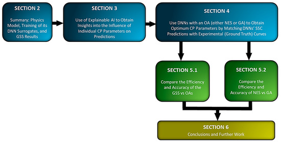
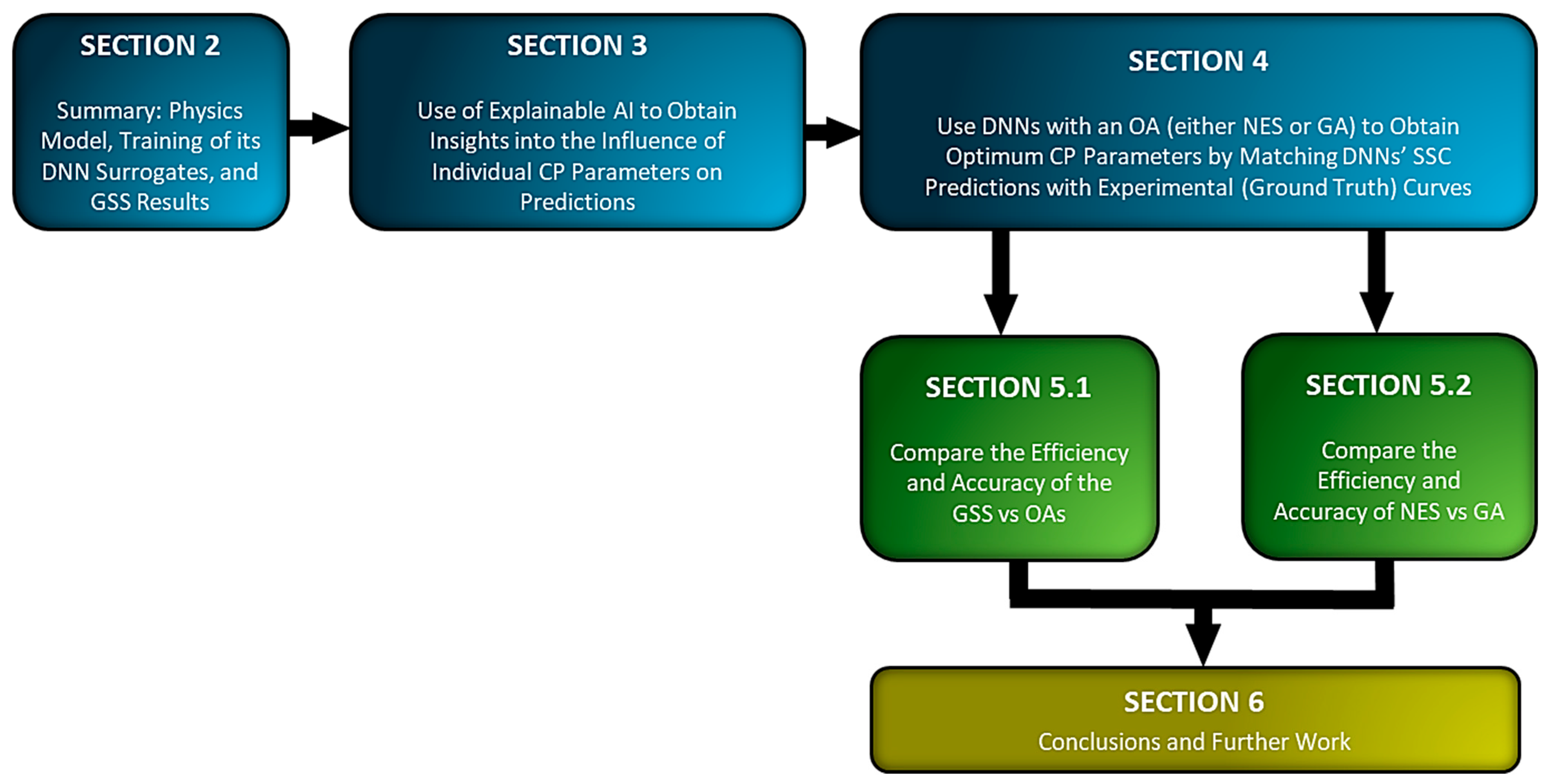
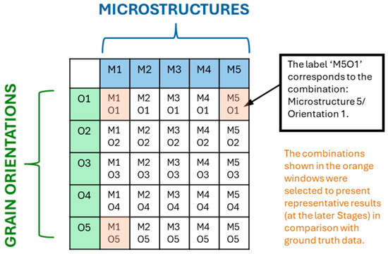
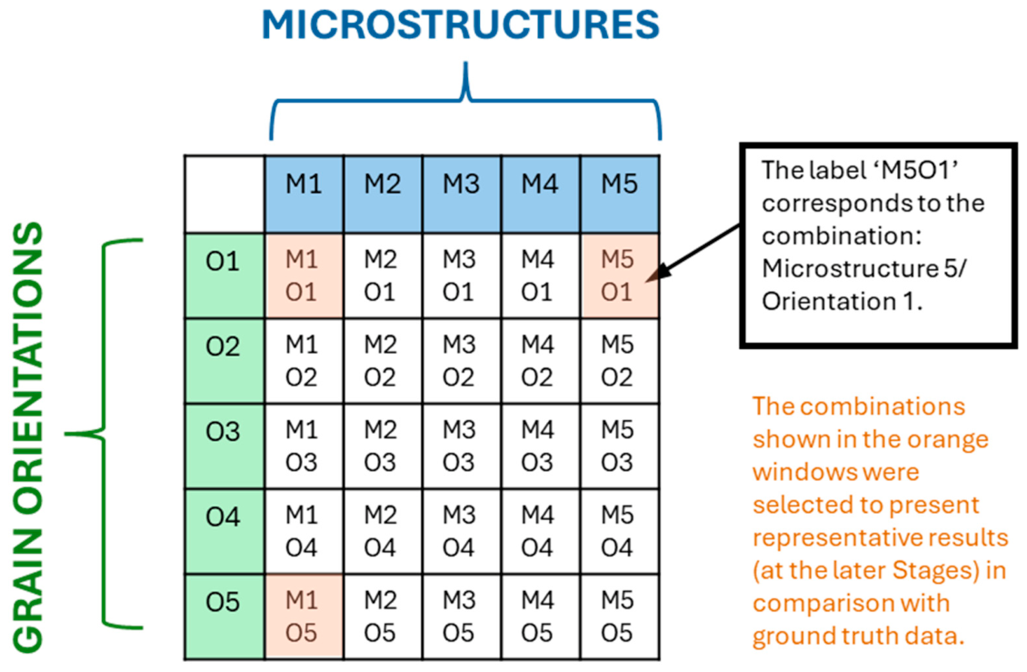
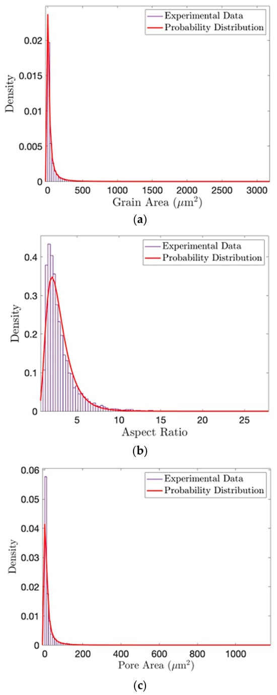
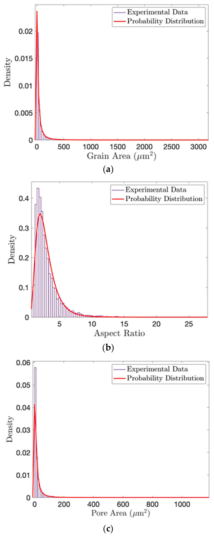
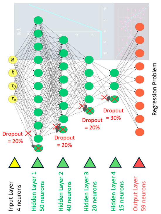
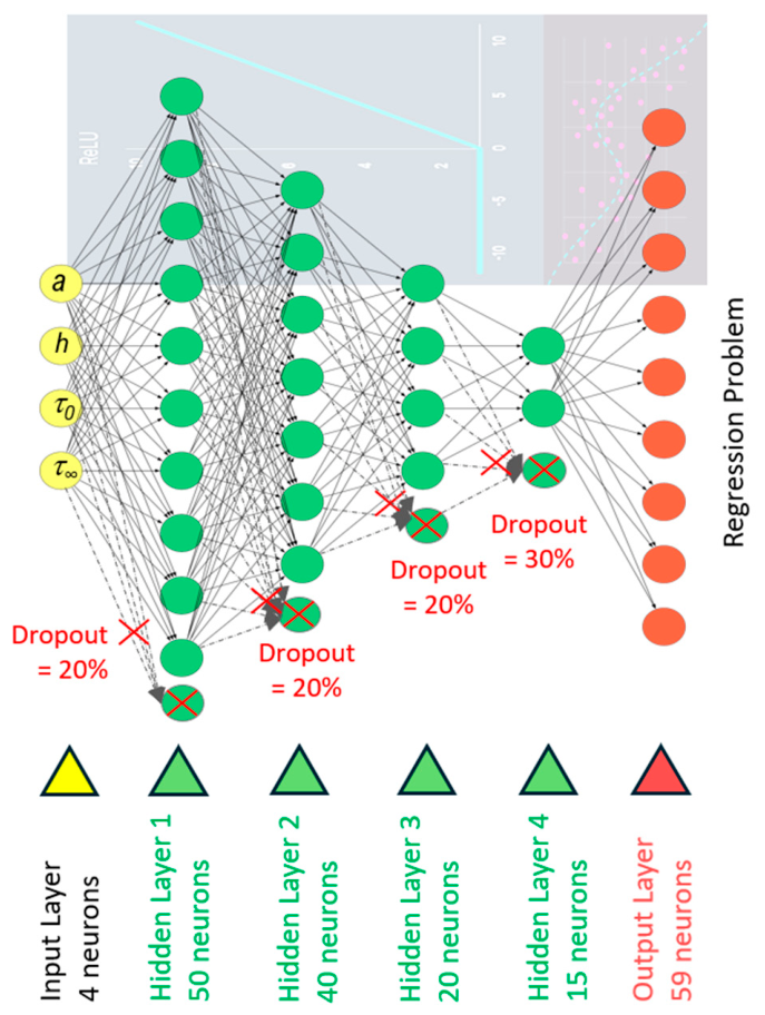
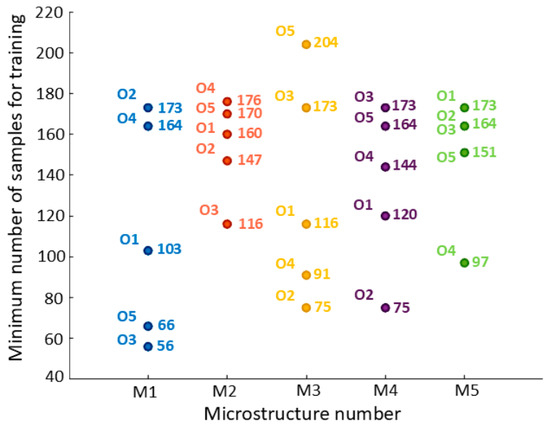
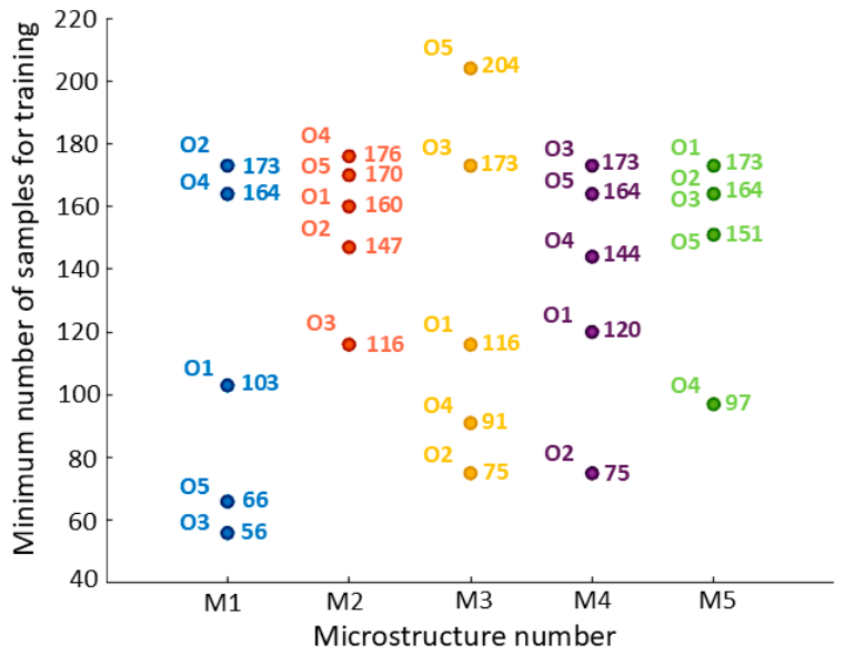
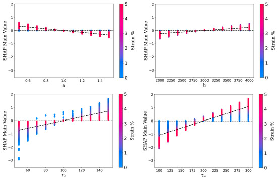
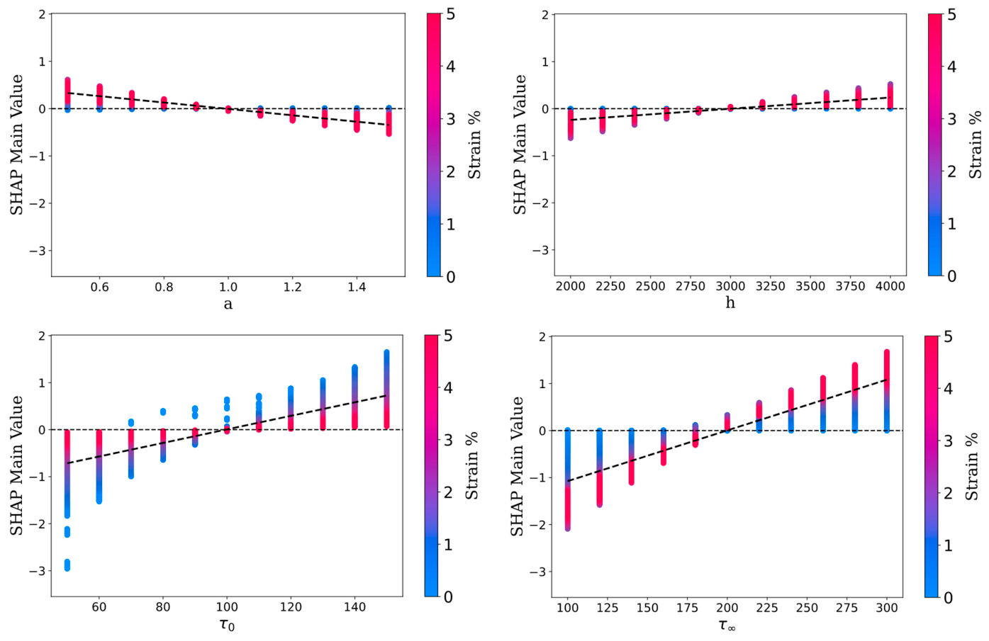
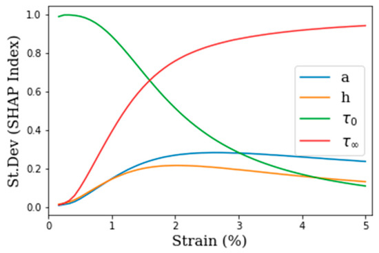
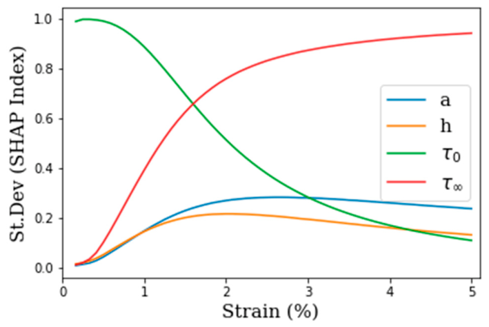
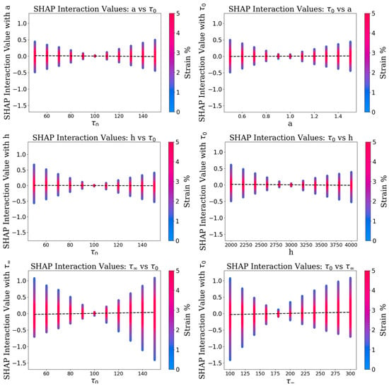
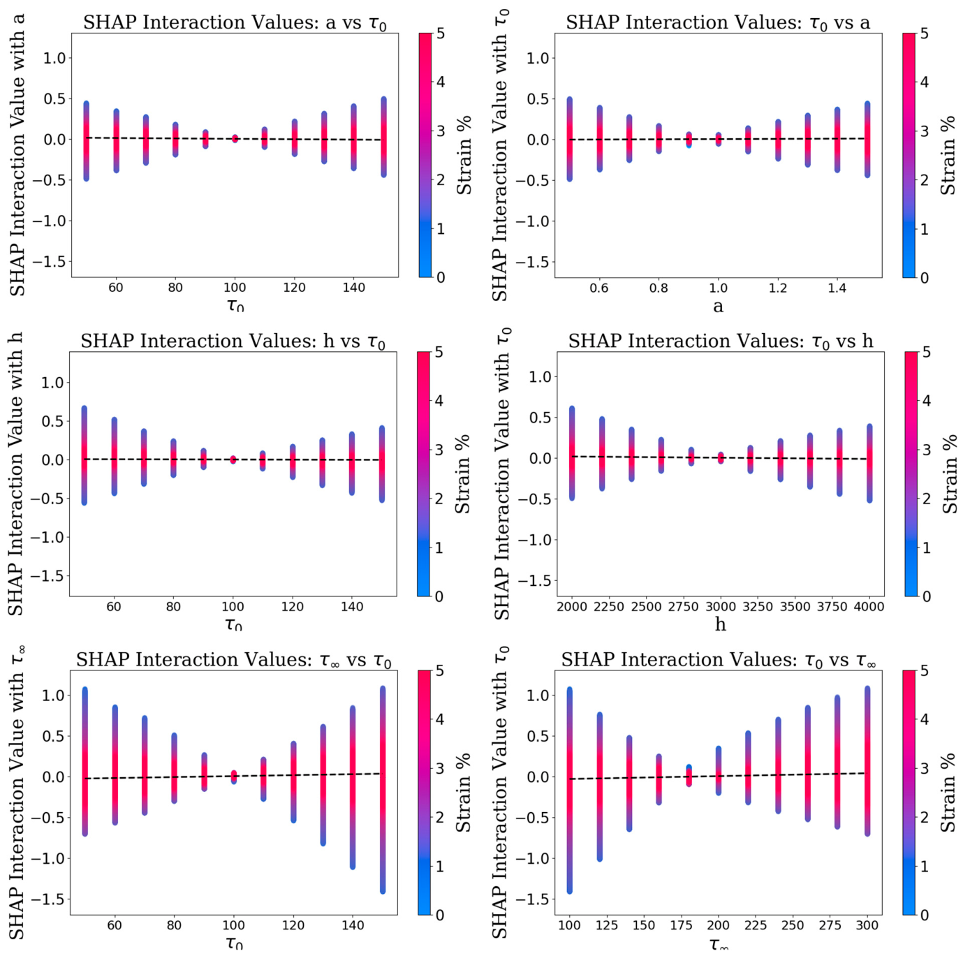
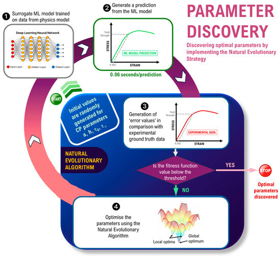
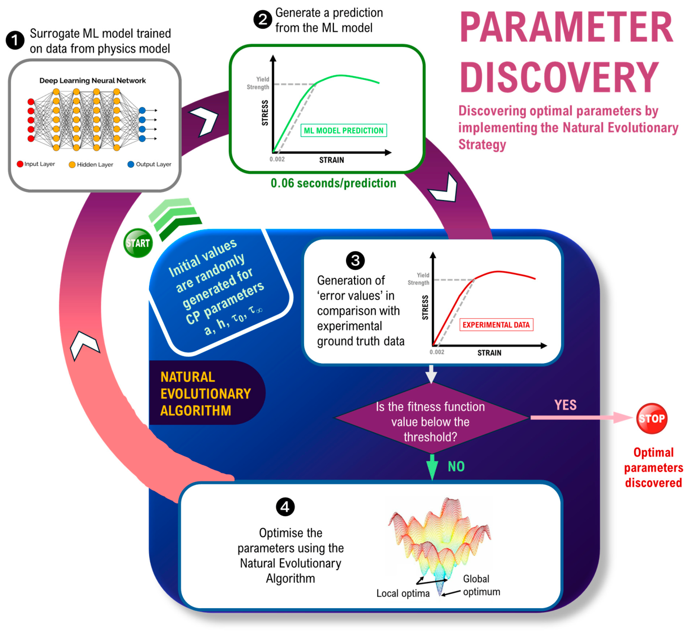
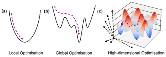
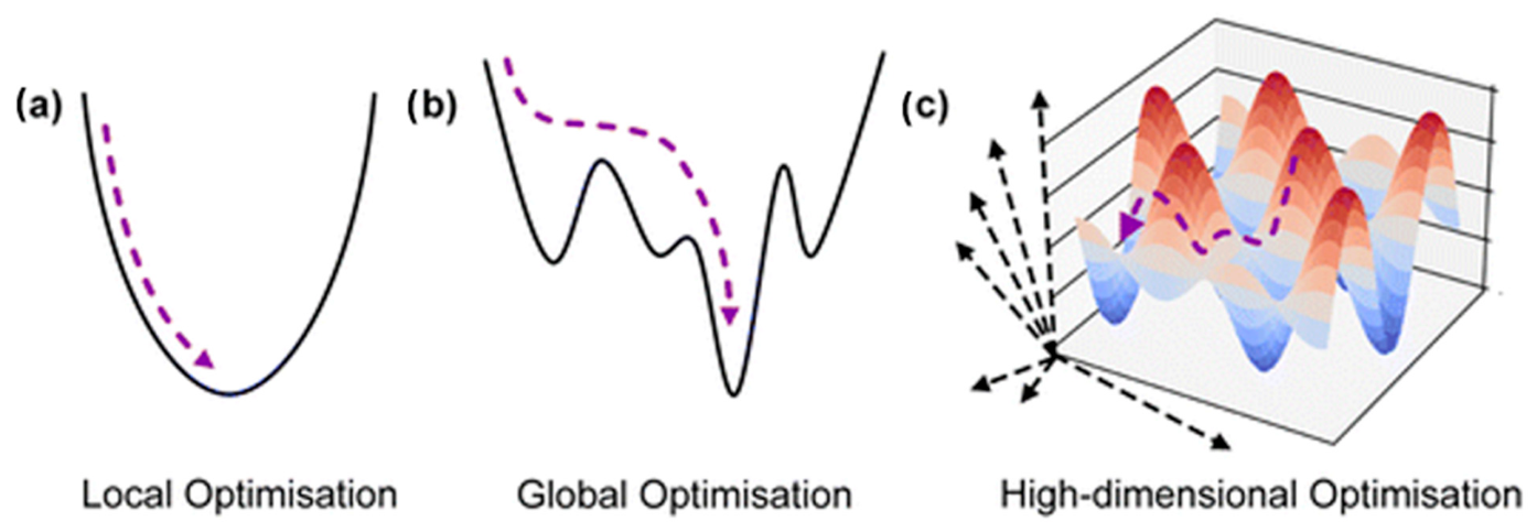
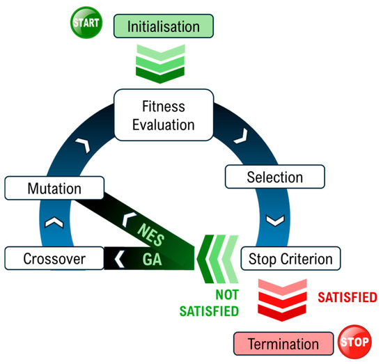
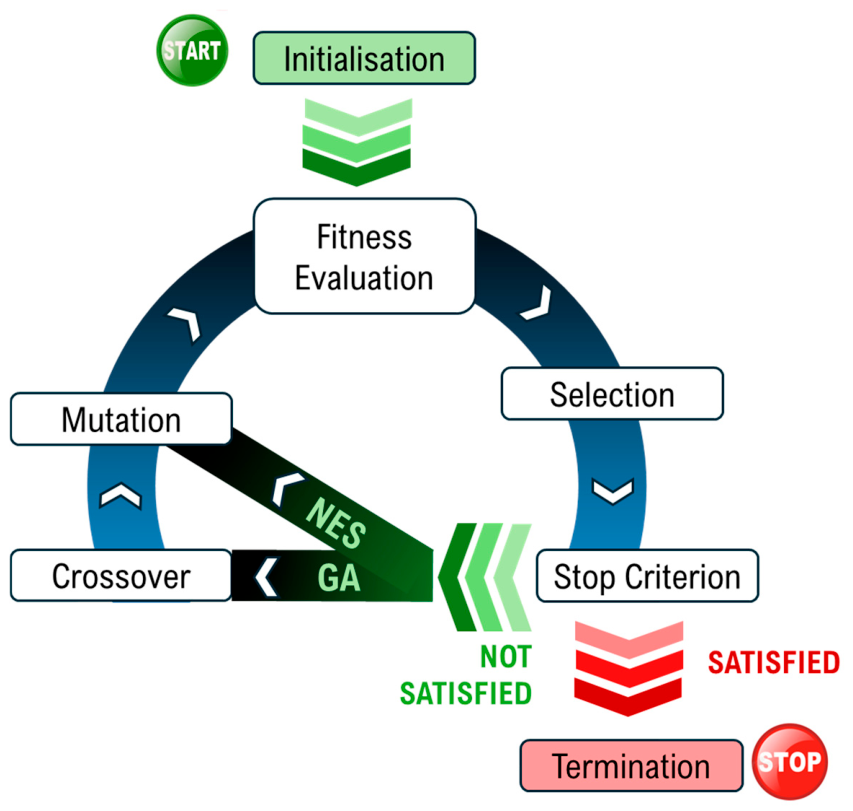
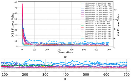
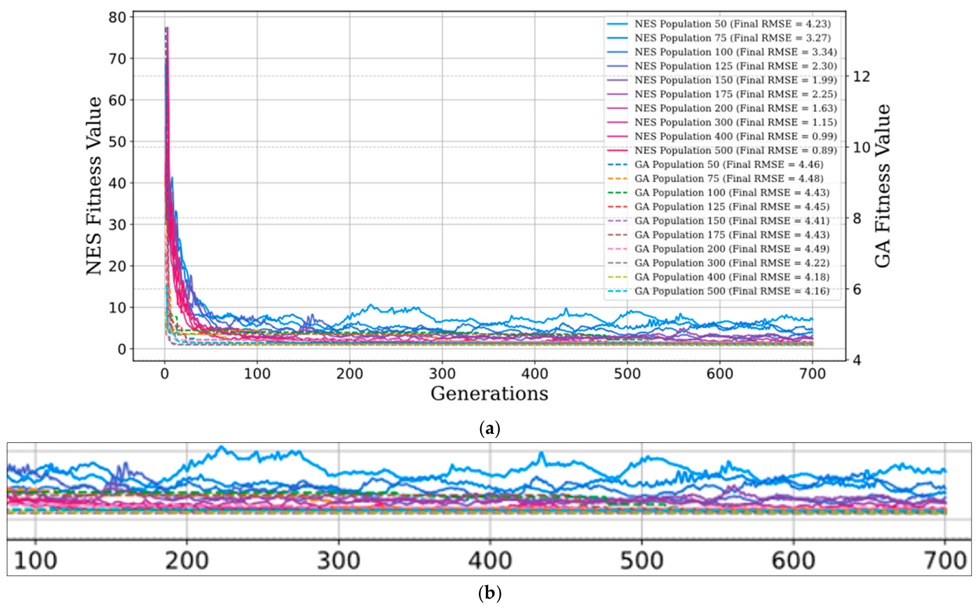
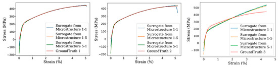
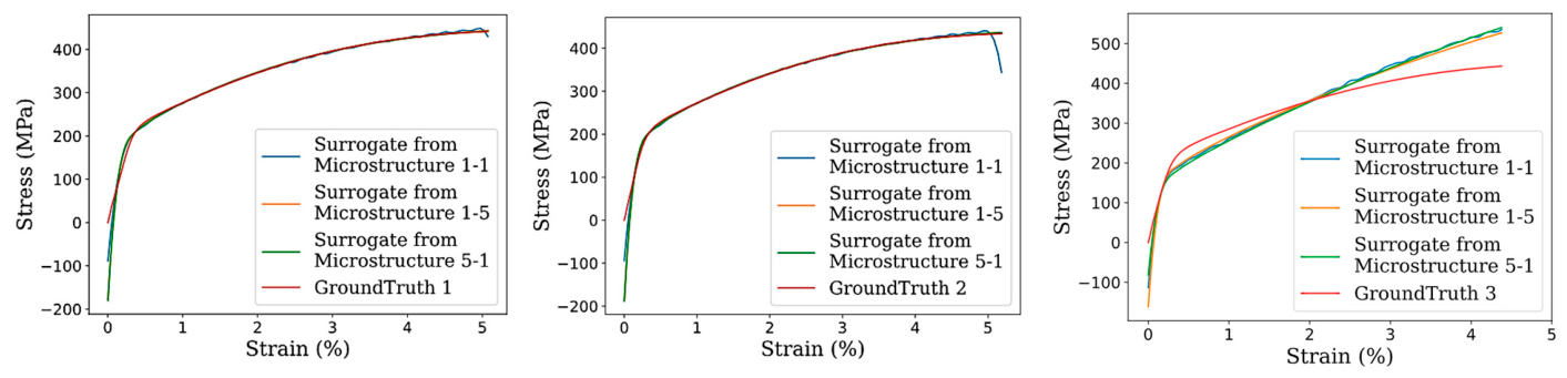
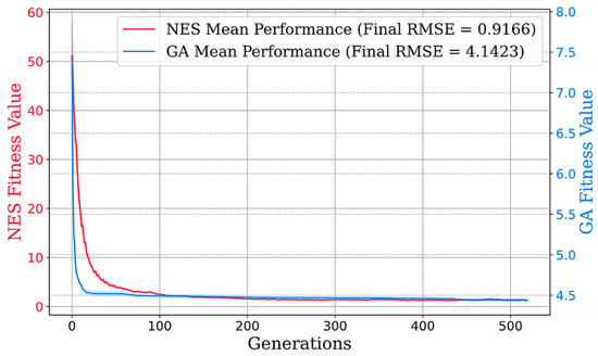
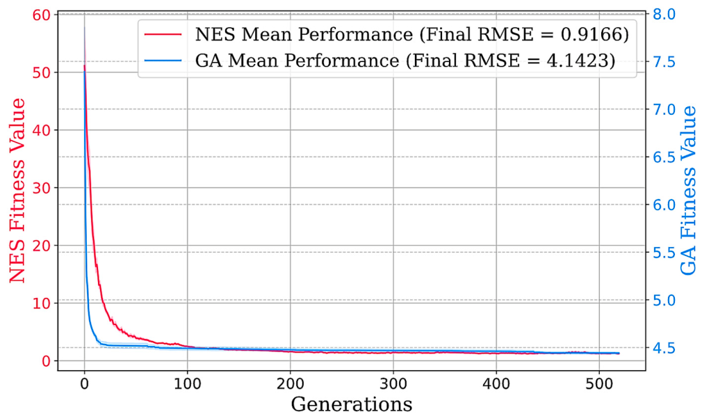
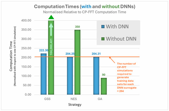
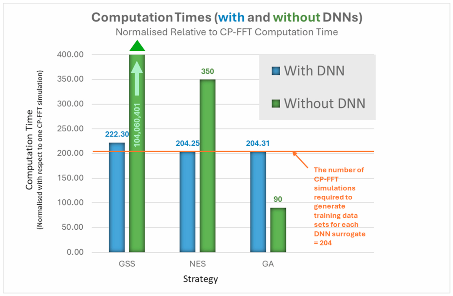

Disclaimer/Publisher’s Note: The statements, opinions and data contained in all publications are solely those of the individual author(s) and contributor(s) and not of MDPI and/or the editor(s). MDPI and/or the editor(s) disclaim responsibility for any injury to people or property resulting from any ideas, methods, instructions or products referred to in the content. |
© 2026 by the authors. Licensee MDPI, Basel, Switzerland. This article is an open access article distributed under the terms and conditions of the Creative Commons Attribution (CC BY) license.