Investigation of Bubble Size and Spatial Distribution in a Continuous Casting Mold Considering Coalescence and Breakup

Abstract

In a steel continuous casting mold, argon bubbles injected through the submerged entry nozzle undergo transport, coalescence, and turbulent breakup, producing a polydisperse bubble swarm that affects flow stability and defect formation. In this study, an Euler–Lagrange model coupled with bubble collision coalescence and turbulence-induced breakup sub-models was established and validated using water model observations. Three daughter-bubble volume distribution models were compared in terms of bubble-cloud morphology, number-fraction distribution, and median-diameter evolution at different gas flow rates. For the median bubble diameter at different gas flow rates, the M-type model gives the lowest mean absolute error of 0.0349 mm. Large bubbles with diameters greater than 2.5 mm accounted for about 4% of the total number and were mainly concentrated near the SEN, whereas small bubbles with diameters of 1.0–1.5 mm accounted for about 60% and were dispersed throughout the upper recirculation region. Mechanism analysis further shows that bubble transport is drag-dominated in the high-velocity jet region, while buoyancy becomes more important in weaker flow regions; turbulent breakup is localized mainly in high-dissipation regions.

1. Introduction

In continuous casting processes, argon gas is typically injected into the inner wall of the submerged entry nozzle (SEN) to suppress excessive inclusion adhesion and air entrainment caused by negative pressure. The injected argon forms bubble clusters in molten steel, whose motion and size evolution significantly influence flow dynamics and defect formation within the mold. Studies [1,2,3,4,5,6,7,8] have demonstrated that bubbles undergo complex size evolution within the mold: small bubbles may collide and coalesce into larger ones, while under intense turbulence and shear forces, these macrobubbles can further fragment into smaller bubbles, resulting in bubble clusters with broad particle size distributions. Additionally, macrobubbles primarily experience buoyancy effects and typically rise near the nozzle to the slag layer for removal. During this process, macrobubbles exert significant traction on the molten steel through interphase forces, driving the surrounding fluid upward and altering the morphology of the upper recirculation zone in the mold. In contrast, small bubbles are predominantly driven by the traction force exerted by the molten steel, move farther away, and may be captured by the solidification front. These unbound bubbles may form porosity defects in the cast slab, and during rolling, uncompacted pores tend to elongate, with the metal layer above some subsurface bubbles thinning or even fracturing, leading to peeling and flaking defects [9,10,11,12]. Therefore, accurately predicting the bubble size distribution (BSD) within the mold, particularly the fragmentation of macrobubbles into smaller ones in the nozzle jet zone due to intense turbulence, is important for evaluating and optimizing continuous casting processes and improving slab cleanliness [13,14].

In the study of bubble breakup behavior, researchers have proposed various distribution models to describe the volume distribution patterns of sub-bubbles after fragmentation. Lehr et al. [15] proposed a model hypothesizing that bubble breakup may generate multiple sub-bubbles of different sizes, resulting in a bimodal M-shaped distribution. Luo and Svendsen [16], based on the theory of turbulent vortex effects, suggested that bubble breakup typically produces two sub-bubbles of unequal volumes, exhibiting a U-shaped distribution. Lee et al. [17] proposed a symmetric distribution model, hypothesizing that bubbles preferentially break uniformly into two sub-bubbles of similar sizes, corresponding to a bell-shaped N-distribution. When two bubbles approach each other, a liquid film forms at their interface, and the drainage process of this film determines the outcome of the collision: if the liquid film thickness remains above a critical value, the bubbles will rebound; if the liquid film is completely drained and ruptured, coalescence occurs. Chesters and Hofman [18] proposed that the Weber number can distinguish these two behaviors, thereby providing a theoretical basis for bubble collision coalescence criteria.

Due to the opacity of molten steel at high temperatures and extreme operating conditions, numerical simulation has become an indispensable tool for investigating this microscopic physical process. Discrete gas–liquid two-phase flow simulations can be categorized into two types based on bubble tracking methods: the Euler–Euler method and the Euler–Lagrange method. The Euler–Euler approach significantly reduces computational costs by analyzing macroscopic statistical properties of bubble clusters rather than tracking individual bubble trajectories. However, its limitation lies in the difficulty of effectively capturing and describing the evolution of bubble clusters with polydisperse size distributions. Additionally, the Euler framework can be combined with the Population Balance Model (PBM) method, which not only handles bubble clustering but also simulates bubble coalescence and breakup processes. Current studies on multi-size bubble flow in mold [2,19,20,21,22] partially adopt this approach. Nevertheless, PBM has notable limitations in practical applications: First, numerical diffusion and discretization errors occur because bubble diameter is a continuous variable, while PBM forces sub-bubbles generated by fragmentation into predefined discrete size bins, leading to loss of precise size information and smoothed distribution curves. Second, historical information is lost as the Euler framework cannot distinguish residence time or origin of bubbles within the same mesh. In contrast, the Euler–Lagrange method independently tracks the motion and evolution of each bubble. Comparative studies show that in predicting bubble behavior in complex metallurgical flow fields, the Euler–Lagrange method typically outperforms the Euler–Euler (PBM) method in matching experimental data regarding bubble dispersion characteristics [23]. In existing Euler–Lagrange-based mold simulations, some studies [24,25] have simplified the process by not modeling bubble coalescence and fragmentation, instead employing artificially defined homogeneous sizes or size distributions. Other studies [26,27], while considering bubble fragmentation, predominantly use equal fragmentation or conventional simplified models. Recent CFD-DBM/VOF, argon-flow, and measurement-based studies have also extended mold-scale descriptions of gas–liquid-slag multiphase behavior and argon transport [28,29,30]. However, few studies have systematically evaluated the sensitivity of predicted bubble size distributions to the choice of daughter size distribution function, and the selection of a breakup model is often made without adequate justification. This gap is particularly consequential in mold simulations, where large and small bubbles influence flow patterns and defect formation through fundamentally different mechanisms.

This study employed the Euler–Lagrange numerical model to simulate bubble flow in a continuous casting mold, incorporating key sub-models such as bubble coalescence and turbulent breakup. Three daughter-size distribution models—the M-type proposed by Lehr et al. [15], the U-type by Luo and Svendsen [16], and the N-type by Lee et al. [17]—were selected for comparative evaluation as they collectively span a representative spectrum of fragmentation outcomes from highly asymmetric breakup to near-equal volume splitting. The results were compared with experimental data from water model tests to conduct an in-depth analysis of critical parameters including bubble distribution, trajectory, and size evolution.

2. Model Description

The Euler–Lagrange framework for gas–liquid two-phase flow is established in this section, with sub-models such as bubble collision and breakup coupled. The main phase flow is solved using the Euler method on a fixed grid, while the Lagrange method is employed to independently track and calculate each bubble. The main assumptions of the present Euler–Lagrange model are summarized as follows: the liquid phase is treated as an incompressible continuous phase and solved in an Eulerian frame; bubbles are tracked as discrete Lagrangian particles represented by an equivalent diameter, with deformation effects included through drag correlations rather than by resolving the gas–liquid interface; bubble-bubble interactions are simplified as binary collision, rebound/coalescence, and swarm-drag correction processes; and bubble breakup is treated as turbulence-induced binary fragmentation, with the daughter-bubble volume distribution prescribed by the selected M-, U-, or N-type model.

2.1. Governing Equations and Turbulence Model of Continuous Phase

The mass and momentum conservation equations for an incompressible fluid in multiphase flow are given as follows:

$${\displaystyle \frac{\partial }{\partial t}}\left({\alpha }_l{\rho }_l\right)+\nabla \cdot \left({\alpha }_l{\rho }_l{\overrightarrow{v}}_l\right)=0$$

(1)

$${\displaystyle \frac{\partial }{\partial t}}\left({\alpha }_l{\rho }_l{\overrightarrow{v}}_l\right)+{\overrightarrow{v}}_l\cdot \nabla \left({\alpha }_l{\rho }_l{\overrightarrow{v}}_l\right)=-\nabla p+\nabla \cdot \left[{\alpha }_l\left({\mu }_l+{\mu }_t\right)\right]\nabla {\overrightarrow{v}}_l+{\overrightarrow{M}}_l$$

(2)

where ${\alpha }_l$ is the volumetric fraction of the liquid phase $p$, ${\rho }_l$ is the density of the liquid phase, ${\overrightarrow{v}}_l$ is the average velocity of the liquid phase, $p$ is the pressure, and ${\overrightarrow{M}}_l$ is the source term of momentum exchange and interacts with the dispersed phase, including resistance, buoyancy, and virtual mass force. ${\mu }_l$ is the viscosity of the liquid phase.

The standard k-ε model was used to describe turbulence. In Equation (2), the turbulent viscosity is represented as ${\mu }_t$, and is calculated as follows:

$${\mu }_t=C_{\mu }{\rho }_l{\displaystyle \frac{k^2}{\epsilon }}$$

(3)

k and ε are solved by the following transport equations.

$${\alpha }_l{\rho }_l\left({\displaystyle \frac{\partial k}{\partial t}}+{\overrightarrow{v}}_l\cdot \nabla k\right)=-\nabla \left({\alpha }_l{\displaystyle \frac{{\mu }_l}{{\sigma }_k}}\nabla k\right)+{\alpha }_l{G}_k-{\alpha }_l{\rho }_l\epsilon$$

(4)

$${\alpha }_l{\rho }_l\left({\displaystyle \frac{\partial \epsilon }{\partial t}}+{\overrightarrow{v}}_l\cdot \nabla \epsilon \right)=-\nabla \left({\alpha }_l{\displaystyle \frac{{\mu }_l}{{\sigma }_{\epsilon }}}\nabla \epsilon \right)+{\alpha }_l{C}_1{\displaystyle \frac{\epsilon }{k}}{G}_k-{\alpha }_l{C}_2{\rho }_l{\displaystyle \frac{{\epsilon }^2}{k}}$$

(5)

$$G_k={\mu }_t\left({\displaystyle \frac{\partial u_{i,j}}{\partial x_j}}+{\displaystyle \frac{\partial u_{i,j}}{\partial x_i}}\right){\displaystyle \frac{\partial u_{i,j}}{\partial x_j}}$$

(6)

The model constants are: $C_{\mu }$ = 0.09, ${\sigma }_k$ = 1.0, ${\sigma }_{\epsilon }$ = 1.3, C₁ = 1.44, C₂ = 1.92.

2.2. Discrete Bubble Model

2.2.1. Bubble Dynamics

Bubbles are considered discrete particles, and their trajectories can be calculated by integrating the following force equation:

$$\begin{array}{l}{\overrightarrow{F}}_{total}=m_b{\displaystyle \frac{d{\overrightarrow{v}}_b}{dt}}=\stackrel{\mathrm{drag}\hspace{0.33em}\mathrm{force}, {\overrightarrow{F}}_D}{\overbrace{C_D{\displaystyle \frac{{\rho }_l\left|{\overrightarrow{v}}_l-{\overrightarrow{v}}_b\right|\left({\overrightarrow{v}}_l-{\overrightarrow{v}}_b\right)}{2}}{\displaystyle \frac{\pi d_b^2}{4}}}}+\stackrel{\mathrm{virtual}\hspace{0.33em}\mathrm{mass}\hspace{0.33em}\mathrm{force}, {\overrightarrow{F}}_{VM}}{\overbrace{{\displaystyle \frac{1}{6}}\pi d_b^3{C}_{VM}{\rho }_l{\displaystyle \frac{d}{dt}}\left({\overrightarrow{v}}_l-{\overrightarrow{v}}_b\right)}}\\ +\stackrel{\mathrm{pressure}\hspace{0.33em}\mathrm{gradient}, {\overrightarrow{F}}_P}{\overbrace{{\displaystyle \frac{1}{6}}\pi d_b^3(-\nabla p+{\rho }_l\overrightarrow{g})}}+\stackrel{\mathrm{gravity}+\mathrm{buoyancy}, {\overrightarrow{F}}_G+{\overrightarrow{F}}_B}{\overbrace{{\displaystyle \frac{1}{6}}\pi d_b^3\left({\rho }_b-{\rho }_l\right)\overrightarrow{g}}}+\stackrel{\mathrm{lift}\hspace{0.33em}\mathrm{force}, {\overrightarrow{F}}_L}{\overbrace{{\displaystyle \frac{1}{6}}\pi d_b^3{C}_L{\rho }_l\left({\overrightarrow{v}}_l-{\overrightarrow{v}}_b\right)\times \left(\nabla \times {\overrightarrow{v}}_l\right)}}\end{array}$$

(7)

where the bubble Reynolds number $R{e}_b={\rho }_l\left|{\overrightarrow{v}}_l-{\overrightarrow{v}}_b\right|d_b/{\mu }_l$, the Eotvos number $Eo=({\rho }_l-{\rho }_g)g{d}_b^2/{\sigma }_{lg}$, the virtual mass force coefficient $C_{VM}=0.5$ and the lift coefficient $C_L=0.5$. The pressure gradient force is calculated by integrating the pressure along the bubble surface area, excluding hydrostatic pressure, which corresponds to buoyancy. Considering the bubble deformation, the applicable drag coefficient model [31,32] is as follows

$$C_D=\max \left[\min \left\{{\displaystyle \frac{16}{Re}}\left(1+0.15R{e}^{0.687}\right),{\displaystyle \frac{48}{Re}}\right\},{\displaystyle \frac{8}{3}}{\displaystyle \frac{Eo}{Eo+4}}\right]$$

(8)

The momentum exchange between the dispersed and continuous phases is treated through two-way coupling. When the liquid phase exerts forces on the bubbles, the corresponding reaction force is applied to the continuous phase as the interphase momentum source.

For bubble swarms, the isolated-bubble drag coefficient was further corrected using the Roghair et al. [33] correlation to account for hindered bubble rise and the increased effective drag at finite gas fractions. Bubble-induced turbulence was considered following the closures reviewed by Zhang et al. [34] and the model of Troshko et al. [35].

2.2.2. Bubble Coalescence and Breakup

When two bubbles move toward each other, the liquid film between them resists their relative motion. If the film thickness exceeds the critical value, the bubbles will rebound upon collision; conversely, if it is below the critical value, the bubbles will coalesce after collision. The study by Chesters and Hofman [18] defined a Weber number to characterize these two behaviors:

$$We={\displaystyle \frac{d_{b,1}{d}_{b,2}{\left[({\overrightarrow{v}}_{b,1}-{\overrightarrow{v}}_{b,2})\cdot {\overrightarrow{I}}_{12}\right]}^2{\rho }_l}{(d_{b,1}+d_{b,2}){\sigma }_{lg}}}$$

(9)

The unit vector represents the direction of the line connecting the centers of bubble 1 and 2, while the velocity indicates the relative motion between particles. Based on Duineveld’s theoretical derivation [36] and experimental studies, this research adopts 0.18 as the critical Weber number, with particles rebounding upon exceeding this threshold and coalescing otherwise. The collision and rebound process between the two bubbles is assumed to be fully elastic. Consequently, the rebounded bubble velocity can be derived from the law of momentum conservation.

When bubbles are in the turbulent region of a macroscopic flow field, the surrounding continuous phase exhibits significant fluctuations and velocity gradients. The resulting shear forces fragment the bubbles into smaller ones. Lehr et al. [15] proposed a model to calculate bubble breakup rates $f\left(d_{b,i}\right)$ and the size distribution of sub-bubbles after fragmentation $\beta \left(f_{bv}\right)$.

$$f\left(d_{b,i}\right)={\displaystyle \frac{d_{b,i}^{5/3}{\epsilon }_l^{19/15}{\rho }_l^{7/5}}{2{\sigma }_{lg}^{7/5}}}\exp \left(-{\displaystyle \frac{\sqrt{2}{\sigma }_{lg}^{9/5}}{d_{b,i}^3{\rho }_l^{9/5}{\epsilon }_l^{6/5}}}\right)$$

(10)

$$\beta \left(f_{bv}\right)={\displaystyle \frac{1}{\sqrt{\pi }{f}_{bv}}}\cdot {\displaystyle \frac{\exp \left\{-\frac{9}{4}{\left[\ln \left(\frac{2^{2/5}{d}_{b,j}{\rho }_l^{3/5}{\epsilon }_l^{2/5}}{{\sigma }_{lg}^{3/5}}\right)\right]}^2\right\}}{\left\{1+\mathrm{erf}\left[\frac{3}{2}\ln \left(\frac{2^{1/15}{d}_{b,i}{\rho }_l^{3/5}{\epsilon }_l^{2/5}}{{\sigma }_{lg}^{3/5}}\right)\right]\right\}}}$$

(11)

where $d_{b,i}$ denotes the diameter of the parent bubble prior to breakup, $d_{b,j}$ denotes the diameter of the smaller daughter bubble after breakup, and $f_{bv}$ is the breakup volume ratio, defined as $d_{b,j}^3/d_{b,i}^3$. Given the computational complexity of solving the inverse function of the cumulative distribution function for this probability distribution, this study employed the Acceptance–Rejection Method to generate random numbers conforming to this probability distribution.

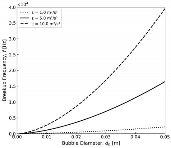
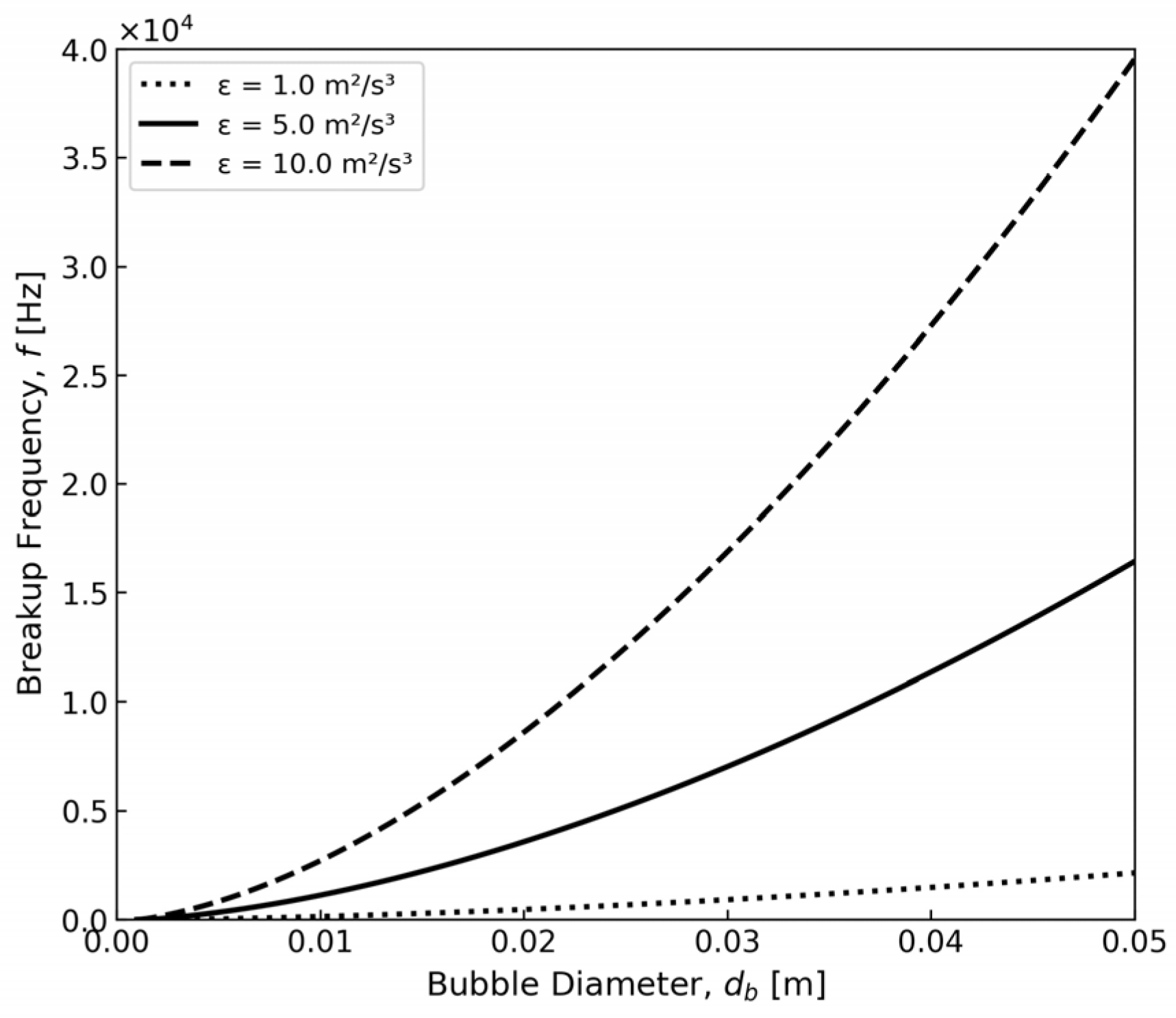
Figure 1 illustrates the variation in bubble breakup frequency with bubble diameter and turbulence dissipation rate, which aligns with the model predictions proposed by Lehr et al. The study reveals that breakup frequency increases significantly with both bubble diameter and turbulence energy dissipation rate (ε). For smaller bubbles (<0.01 m), the breakup frequency remains relatively low, whereas larger bubbles exhibit a steep upward trend, particularly at higher turbulence intensities.

Figure 1. Relationship between bubble breakup rate and turbulent kinetic energy.

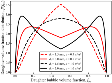
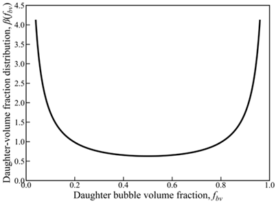
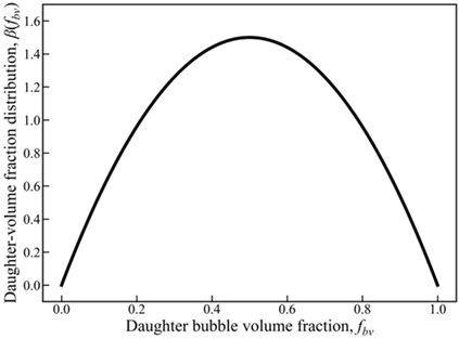
As shown in Table 1, this study compared three commonly used binary bubble volume fraction distribution functions (beta, f_bv) for fragmentation, where f_bv represents the proportion of one of the two daughter bubbles in the parent-bubble volume (0 < f_bv < 1). Lehr et al. [15] observed an “M-shaped” distribution, with higher probabilities at moderately asymmetric splitting (f_bv approximately 0.2–0.3 and 0.7–0.8) and lower probabilities at perfectly symmetric splitting (f_bv = 0.5). Following Luo and Svendsen [16], the U-shaped daughter-volume distribution favors highly asymmetric breakup and was implemented by Sungkorn et al. [37] in an Euler–Lagrange stochastic bubble-parcel model. This formulation is adopted in the present study. Lee et al. [17] documented a unimodal “N-shaped” distribution (approximately normal), with maximum probability near f_bv = 0.5, showing a preference for near-equal-volume splitting.

Table 1. Models of daughter-size distribution after binary bubble fragmentation.

Researcher	Model	Image	Type
Lehr et al. (2002) [15]	$\beta \left(f_{bv}\right)={\displaystyle \frac{1}{\sqrt{\pi }{f}_{bv}}}\cdot {\displaystyle \frac{\exp \left\{-\frac{9}{4}{\left[\ln \left(\frac{2^{2/5}{f}_{bv}^{1/3}{d}_i{\rho }_l^{3/5}{\epsilon }^{2/5}}{{\sigma }^{3/5}}\right)\right]}^2\right.}{\left\{1+\mathrm{erf}\left[\frac{3}{2}\ln \left(\frac{2^{1/15}{d}_i{\rho }_l^{3/5}{\epsilon }^{2/5}}{{\sigma }^{3/5}}\right)\right]\right.}}$		M
Sungkorn et al. (2011) [37], based on Luo and Svendsen (1996) [16]	$f_{bv}={\displaystyle \frac{1}{2}}+{\displaystyle \frac{1}{2}}\tanh (10(x-(1/2))/\mathrm{\pi })$ where x is a uniform random number in [0, 1]		U
Lee et al. (1987) [17]	$\beta \left(f_{bv}\right)={\displaystyle \frac{\mathrm{\Gamma }(4)}{\mathrm{\Gamma }(2)\mathrm{\Gamma }(2)}}{f}_{bv}\left(1-f_{bv}\right)$		N

3. Experimental Setup and Procedure

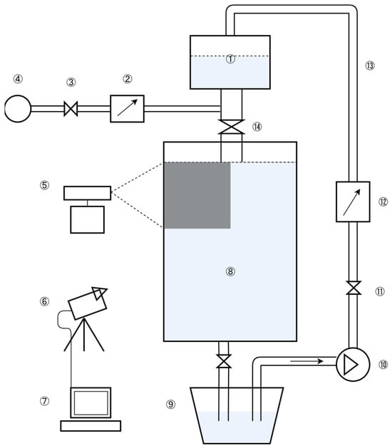
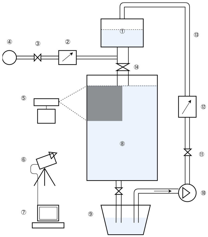
The experimental setup (Figure 2) primarily consisted of a water model fluid-control system and an image-acquisition system. The dimensions of the water model and parameters such as the gas–liquid two-phase flow rates were determined based on geometric and dynamic similarity. High-speed cameras were used to capture images, which were then processed using Image Pro Plus 6.0 image-analysis software. The cameras were positioned directly in front of the wide surface of the mold, with two 1000 W halogen lamps serving as illumination sources. Images were captured at an exposure time of 10 ms and a frame rate of 100 frames per second. After being transmitted to the computer, the images were processed to measure bubble-motion parameters and analyze bubble trajectories.

Figure 2. Schematic diagram of the experimental apparatus. 1. Tundish; 2. Gas flow meter; 3. Valve; 4. Air compressor; 5. Laser light source; 6. High-speed camera; 7. Computer; 8. Mold; 9. Water tank; 10. Water pump; 11. Valve; 12. Liquid flow meter; 13. Water pipe; 14. SEN.

The water model experiment was designed according to geometric and dynamic similarity principles. The geometric scale ratio between the water model and the prototype caster is $\lambda =L_m/L_p=0.6$, where the subscripts m and p denote the water model and the prototype, respectively. The main flow in the mold is governed primarily by the balance between inertial and gravitational forces. Therefore, following common water model practice for continuous-casting molds, the liquid flow rate was determined by matching the Froude number:

$$Fr={\displaystyle \frac{u^2}{gL}}$$

(12)

For geometrically similar systems, Froude similarity gives

$${\displaystyle \frac{Q_m}{Q_p}}={\lambda }^{2.5}\approx 0.2789$$

(13)

The liquid flow rate in the water model was therefore selected according to this target flow-rate ratio. Using the effective SEN outlet areas reported in the water model design data, the corresponding characteristic Froude numbers of the water model and prototype are approximately 0.947 and 0.944, respectively. The estimated Reynolds numbers are of the order of 10⁴ for both systems, indicating that both the model and prototype operate in the fully turbulent regime. Under this condition, the mismatch in the exact Reynolds number has a limited influence on the similarity of the main flow structure.

For the gas phase, the density difference between liquid and gas must be considered. Therefore, the gas flow rate was determined using the modified Froude number:

$${Fr}_m^{\prime }={\displaystyle \frac{{\rho }_g{u}_g^2}{\left({\rho }_l-{\rho }_g\right)gL}}$$

(14)

where $u_g$ is the characteristic gas velocity at the SEN outlet. The thermal expansion of argon gas after entering molten steel was considered using the ideal-gas relation. By imposing the same modified Froude number for the model and prototype, and using $Q_g=A{u}_g$ and $A_m/A_p={\lambda }^2$, where $A_m$ and $A_p$ are the corresponding flow cross-sectional areas used to define the model and prototype gas velocities, respectively, the gas flow-rate ratio can be written as

$${\displaystyle \frac{Q_{g,m}}{Q_{g,p,0}}}={\displaystyle \frac{T_p}{T_0}}{\lambda }^{2.5}{\left[{\displaystyle \frac{{\rho }_{g,p}\left({\rho }_{l,m}-{\rho }_{g,m}\right)}{{\rho }_{g,m}\left({\rho }_{l,p}-{\rho }_{g,p}\right)}}\right]}^{1/2}\approx 0.31$$

(15)

Here, $Q_{g,m}$ and $Q_{g,p,0}$ denote the model gas flow rate and the prototype room-temperature gas flow rate, respectively, and $T_p$ and $T_0$ are the prototype gas temperature and room temperature, respectively. Therefore, the target air flow rate in the water model is approximately 0.31 times the corresponding room-temperature argon flow rate in the prototype system. The gas flow rate in the present water model experiment was set according to this modified-Froude scaling relation.

In addition to the mold-scale Froude similarity discussed above, surface tension is important for bubble deformation, coalescence, and breakup. Since the interfacial tension of molten steel-argon is much higher than that of water-air, direct one-to-one similarity at the bubble scale cannot be fully achieved. However, this difference mainly affects the absolute breakup rate through model inputs such as the Weber-number-related terms, rather than the structural comparison among daughter-size distribution models. The M-, U-, and N-type distributions differ primarily in their assumptions regarding the final breakup configuration of the parent bubble: bimodal breakup controlled by turbulent forcing, highly asymmetric breakup, and nearly equal-volume breakup, respectively. Therefore, the water model remains suitable for providing an observable and dynamically scaled mold-flow environment to compare the relative effects of different daughter-size distribution assumptions on bubble size evolution and spatial distribution, while the steel-argon properties are used as prototype reference values for interpreting the scalability and limitations of the bubble-scale sub-models.

4. Simulation Conditions and Procedure

This study used a three-dimensional Euler–Lagrange method to simulate gas–liquid two-phase flow in a steel continuous casting mold. All parameters listed in Table 2, including those of the water model and prototype, are defined consistently to ensure direct comparison between the experimental and numerical results.

Table 2. Geometric and process parameters of water model and prototype.

Parameter	Water Model	Prototype
Width × Thickness of the mold (mm)	420 × 108	700 × 180
Outlet angle (degree)	12	12
Height and width of the SEN port (mm)	36 × 24	60 × 40
SEN immersion depth (mm)	96	160
Liquid density (kg/m3)	1000	7020
Gas density (kg/m3)	1.138	0.56
Liquid viscosity (N·s/m2)	0.001	0.0056
Liquid flow rate (m3/h−1)	1.48	5.3
Gas volume flow rate (m3/h−1)	0.037, 0.074, 0.112	0.12, 0.24, 0.36
Interfacial tension (N/m)	0.072	1.5

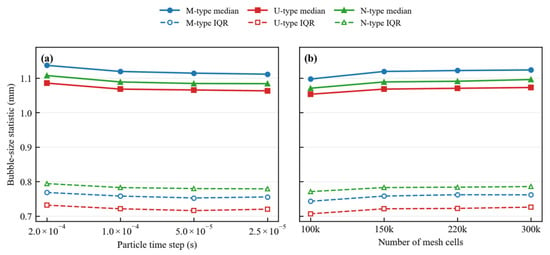
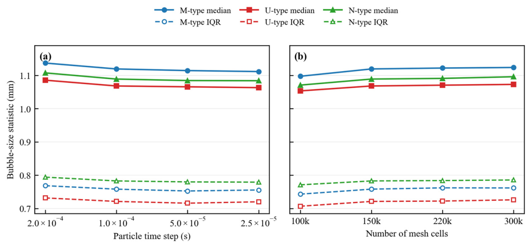
The Eulerian framework for the aqueous phase was solved using the commercial CFD software Ansys Fluent 18.1, while the Lagrangian framework for bubbles was implemented using self-developed code. During each computational time step, interaction information was exchanged through user-defined functions (UDFs). Specifically, when a computational cell containing bubbles was identified, the system retrieved local fluid velocities and other mesh data through UDFs to calculate bubble motion, coalescence, and breakup. The feedback effect of bubbles on the continuous phase was then introduced through user-defined source terms. Fluent used double-precision floating-point operations with a convergence tolerance of 0.0001. The simulation domain was divided into 150,000 mesh cells, and further mesh refinement did not significantly alter the simulation results. After repeated testing and consideration of computational cost and accuracy, the final time steps for the Eulerian and Lagrangian phases were set to 0.0005 s and 0.0001 s, respectively.

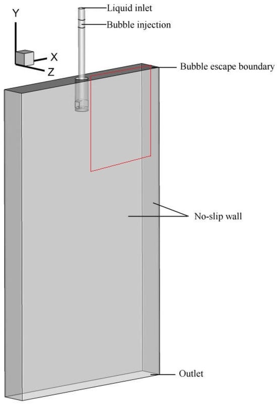
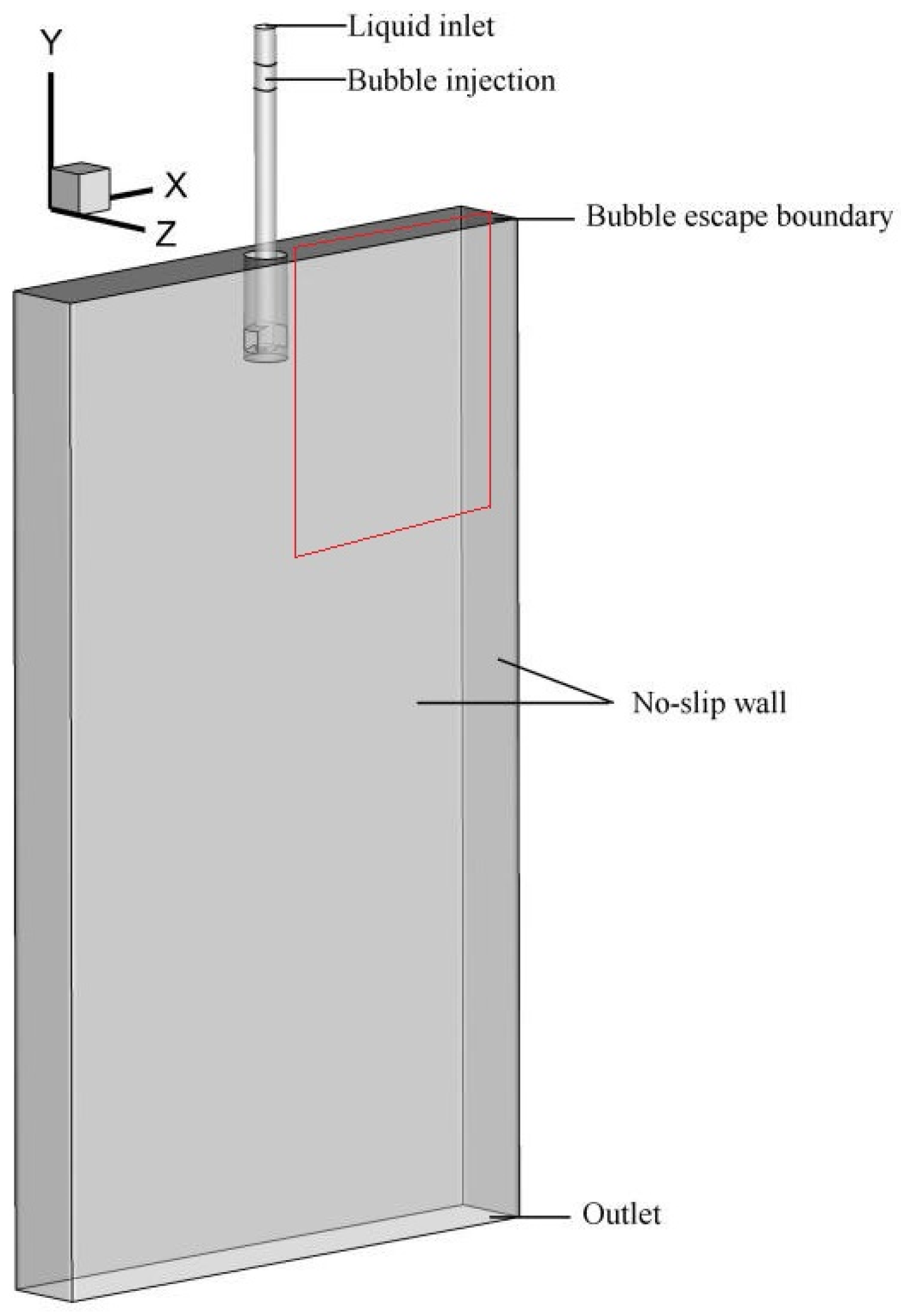
The liquid-phase boundary conditions were configured as follows. As shown in Figure 3, the liquid inlet was set as a mass-flow inlet. Bubbles were introduced from the inner wall of the submerged nozzle. The water model sidewall and nozzle wall were set as a liquid no-slip wall and a bubble bounce wall, respectively. The top surface served as both the gas-phase outlet and the free-slip wall for the liquid. The initial diameter of the injected bubbles was 1.0 mm.

Figure 3. Schematic diagram of the geometric structure and boundary conditions of the simulation domain.

As shown in Figure 4, the current simulation setting is 1.0 × 10⁻⁴ s for the particle time step and 150,000 mesh cells. The results for the M-, U-, and N-type breakup models show only minor changes over the tested ranges, indicating that the selected numerical settings have a limited influence on the present bubble-size statistics.

Figure 4. Sensitivity of bubble-size statistics to numerical settings at a gas volume flow rate of 0.037 m³/h. (a) Effect of particle time step at 150,000 mesh cells. (b) Effect of mesh resolution at a particle time step of 1.0 × 10⁻⁴ s. Solid lines denote the median bubble diameter, whereas dashed lines denote the interquartile range (IQR) of the bubble diameter distribution.

5. Results and Discussion

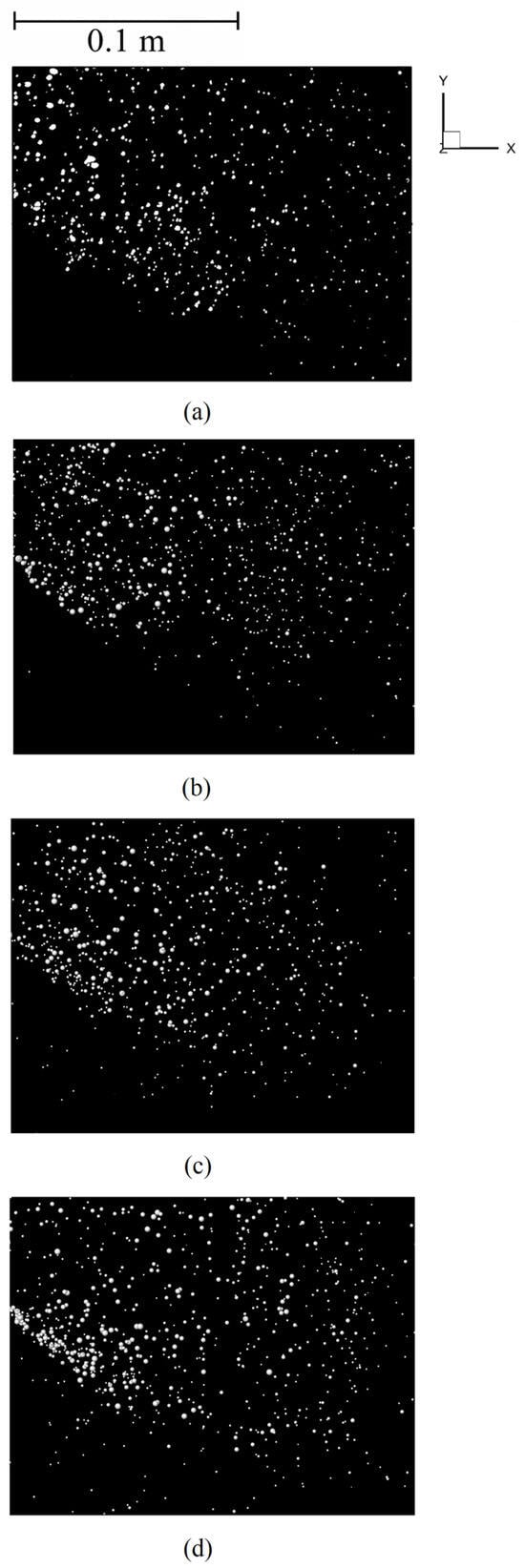
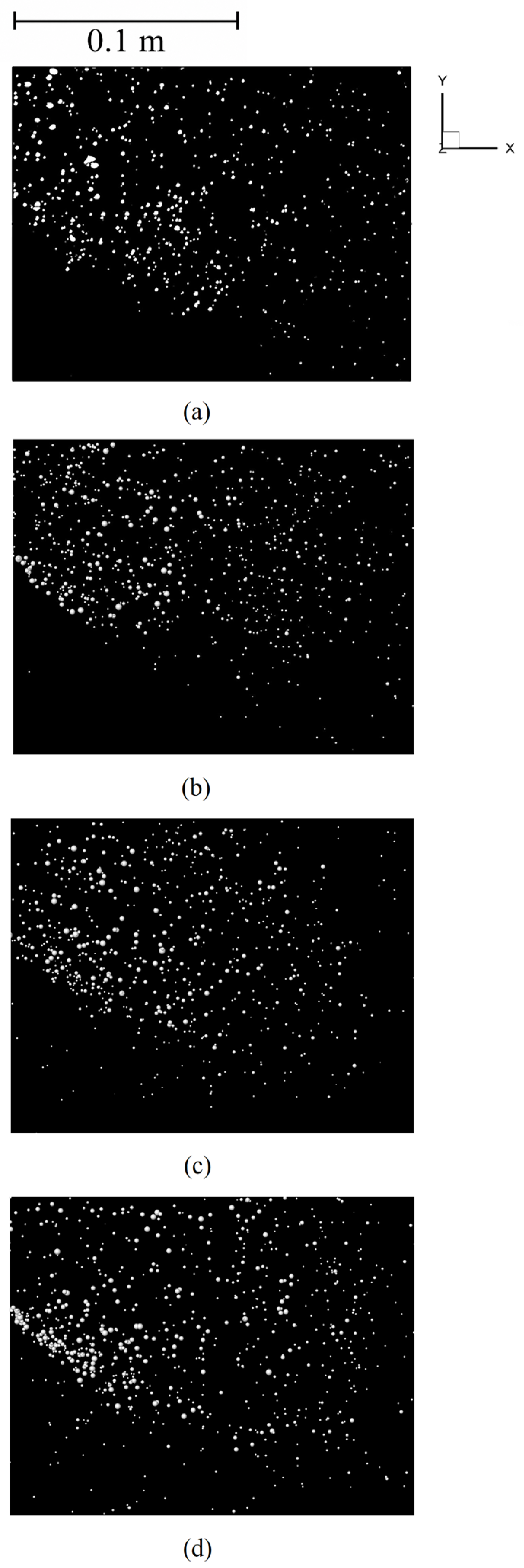
Figure 5 visually compares the experimentally observed bubble distribution with simulations from three fragmentation models. The left panel shows the nozzle exit region, while the right panel depicts the narrow wall area. (a) The water model experiment reveals that bubbles, after exiting the nozzle, diffuse toward the narrow wall (right) with the jet action. Due to fragmentation and coalescence, the flow field contains both large bubbles and numerous fine sub-bubbles, forming a continuous bubble cloud.

Figure 5. Comparison of bubble distributions between the water model experiment and numerical simulations at a gas volume flow rate of 0.037 m³/h. The region shown corresponds to the boxed area in Figure 3, with an additional 20 mm region near the liquid surface cropped out to avoid edge interference caused by free-surface fluctuations. (a) Water model experiment; (b) M-type; (c) U-type; (d) N-type.

Comparison of Figure 5b with the experimental result in Figure 5a shows that the simulated bubble cloud from the M-type model most closely matches the observed morphology, density, and coexistence of bubble sizes in the water model experiment. The U-type fragmentation model assumes that a bubble tends to fragment into a tiny microbubble and a larger bubble similar to the parent bubble. Figure 5c shows that the field of view is filled with extremely fine dot-like bubbles and fewer medium-sized bubbles, resulting in an excessively dense bubble cloud that deviates from the experimentally observed diversity of bubble sizes. The N-type fragmentation model assumes that bubbles tend to split into two nearly equal-sized daughter bubbles. Figure 5d shows fewer fine bubbles than the experimental result, and the overall bubble-size distribution is more uniform, with bubble sizes tending to be larger.

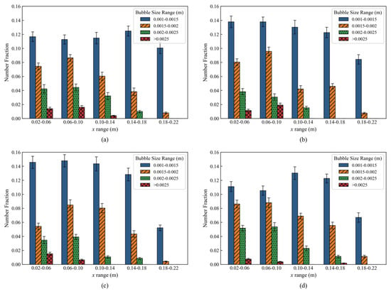
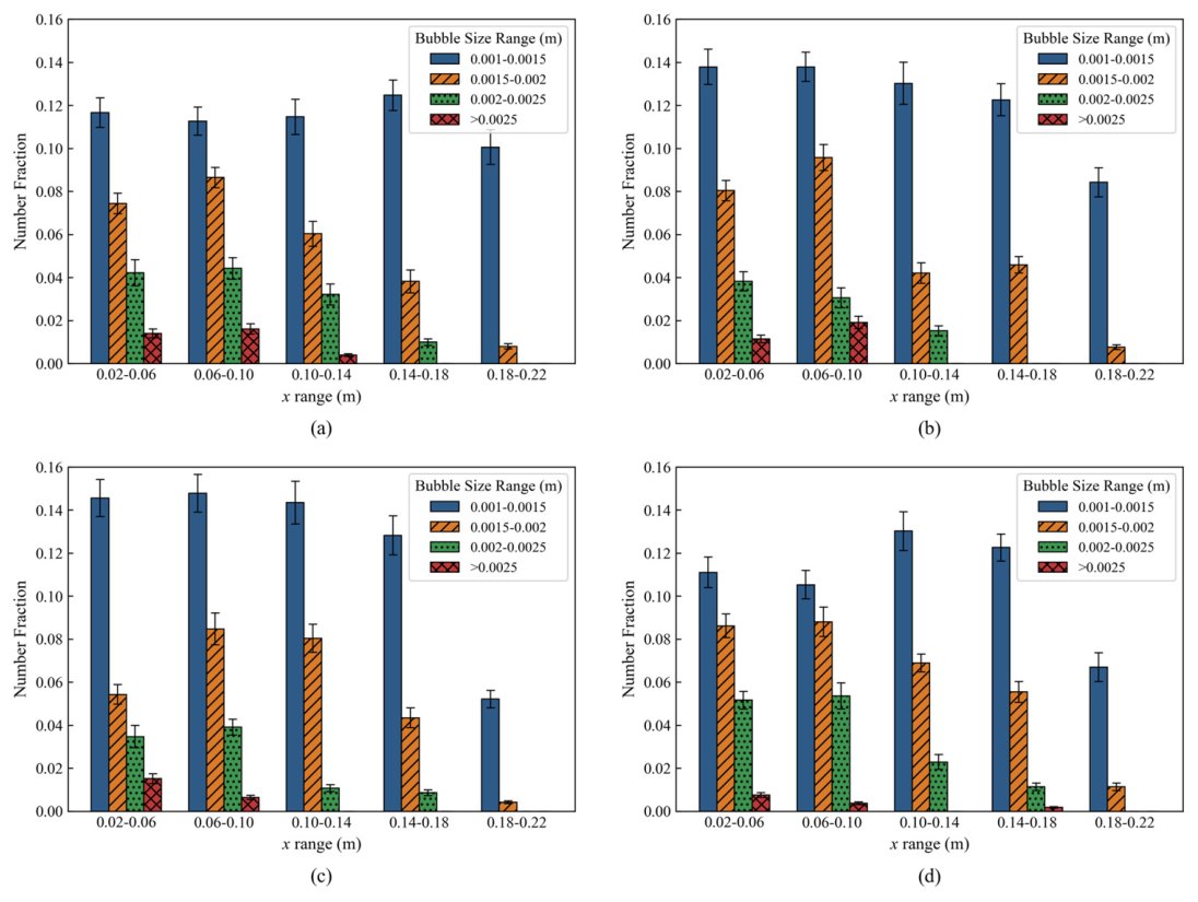
To further support the visual comparison of the breakup models shown in Figure 5, the same experimental and simulated bubble distributions were statistically analyzed in Figure 6. Figure 6 quantifies the bubble number fraction in different horizontal positions (x range, representing the distance from the SEN center) and bubble size classes. The distribution was first normalized within each x-bin and within each size-bin to avoid bias from high-occupancy bins, and the TVD was then calculated for the normalized distributions. The resulting balanced TVD values are 0.0863 for M-type, 0.1136 for U-type, and 0.0953 for N-type, indicating that M-type shows the best quantitative agreement with the experiment. Small bubble distribution (0.001–0.0015 m, blue bars): U-type (Figure 6c): Due to the U-type fragmentation mechanism’s tendency to generate microsatellite bubbles, the simulation results show significantly higher proportions of microbubbles (blue bars) across all regions compared to experimental values (Figure 6a), exhibiting excessively high fraction values (approaching 0.15). N-type (Figure 6d): The N-type model’s preference for isovolumetric fragmentation suppresses microbubble formation. Statistical results demonstrate markedly lower microbubble proportions than experimental values (e.g., in the x = 0.02–0.06 range, experimental value ~0.12 vs. N-type ~0.11), with rapid decline in microbubble proportions as distance increases. M-type (Figure 6b): The M-type model’s predicted microbubble distribution trends align well with experimental data, ensuring sufficient microbubble generation without the excessive generation predicted by the U-type model. Large and medium-sized bubbles (>0.0015 m, orange/green/red bars): Experimental results (a) show that the proportion of large bubbles (red/green bars) decreases gradually with increasing distance from the SEN (x), consistent with the physical process of large-bubble flotation and fragmentation into microbubbles. In the U-type model (c), the proportion of medium-sized bubbles (orange) is “diluted” by excessive microbubbles due to normalization, resulting in lower representation. The N-type model (d) shows reasonable performance in capturing the persistence of large bubbles but fails to accurately reflect the high proportion of small bubbles. In contrast, the M-type model (b) effectively captures this variation pattern: near the SEN region (x = 0.02–0.06), the size distribution of bubbles aligns well with experimental data; in the region farther from the SEN, the decay trend of large and medium-sized bubbles is also accurately predicted.

Figure 6. Statistical analysis of bubble size and spatial distribution in the upper part of the mold. Gas volume flow rate = 0.037 m³/h. Error bars represent the standard deviations calculated from ten snapshots, with each snapshot treated as one independent sample. (a) Experimental results. (b) M-type breakup model. (c) U-type breakup model. (d) N-type breakup model. Here, x denotes the horizontal distance relative to the centerline of the submerged nozzle.

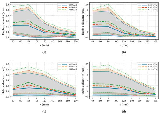
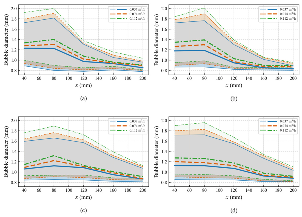
Figure 7 compares the experimental and predicted bubble-size statistics at three gas flow rates. The median bubble diameter and interquartile interval were calculated in five horizontal bins from x = 40 mm to x = 200 mm. To quantify the agreement between simulation and experiment, the mean absolute error (MAE) of the median bubble diameter was calculated over all gas flow rates and horizontal positions. The M-type model gives the lowest MAE of 0.0349 mm, whereas the U-type and N-type models give MAE values of 0.0807 mm and 0.0657 mm, respectively. Therefore, the M-type daughter-size distribution provides the best overall prediction of the central bubble-size trend at variable gas flow rates.

Figure 7. Statistical analysis of bubble size and spatial distribution in the upper part of the mold at different gas volume flow rates. The thick lines represent the median bubble diameter, and the shaded regions indicate the interquartile interval (Q1–Q3). The gray area is an overlapping shaded region of the Q1–Q3 bands. (a) Experimental results. (b) M-type breakup model. (c) U-type breakup model. (d) N-type breakup model (where x denotes the horizontal distance relative to the centerline of the submerged nozzle).

The experimental results show that the median bubble diameter is generally larger near the SEN region and decreases toward the narrow-face side. As the gas flow rate increases from 0.037 to 0.112 m³/h, the median bubble diameter shifts upward, and the interquartile interval becomes wider, especially near the SEN. The M-type model captures this trend more consistently than the U-type and N-type models. Although the U-type and N-type models can approach the experimental median diameter in some downstream positions, they show larger deviations in the near-SEN and intermediate regions, where bubble coalescence and breakup are more intense.

This gas-flow-rate dependence reflects the coupled effects of gas holdup, collision-induced coalescence, turbulent breakup, buoyancy-driven rise, and liquid-phase convection. A higher gas flow rate increases the local bubble number density and collision frequency, which promotes coalescence. Meanwhile, stronger gas–liquid momentum exchange near the SEN enhances local turbulence and promotes breakup. Therefore, the final bubble-size distribution is governed by the local competition between coalescence and breakup, together with buoyancy-driven separation and convective transport. The better performance of the M-type model suggests that a bimodal daughter-size distribution is more suitable for representing this mixed mechanism because it allows both small daughter bubbles generated by turbulent breakup and relatively large residual bubbles to coexist.

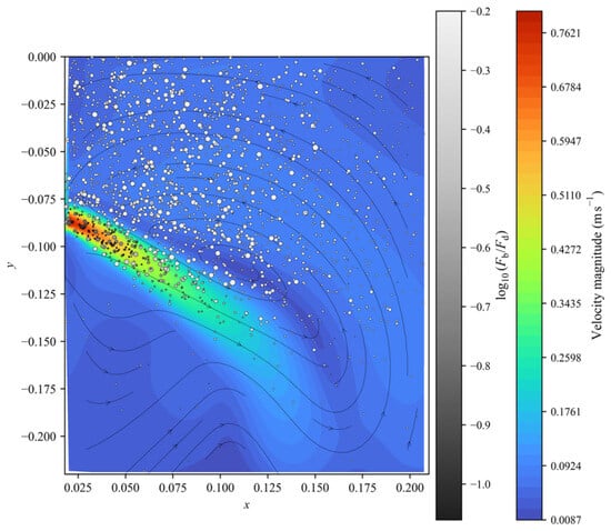
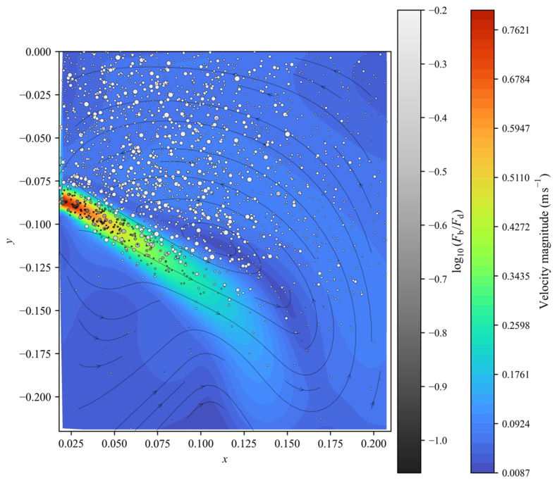
Figure 8 shows that the high-velocity region is concentrated along the jet path and then weakens as the flow enters the upper recirculation region. In the high-speed zone, the bubble cloud follows the liquid-flow direction indicated by the streamlines, showing that drag from the mainstream is the dominant transport mechanism. Away from the jet, the liquid velocity decreases and the relative importance of buoyancy becomes more apparent, as reflected by the spatial variation of log10(F_b/F_d) on the bubble markers. Therefore, large bubbles tend to rise and separate from the main flow more readily, whereas small bubbles remain widely dispersed because their motion is more strongly coupled with the surrounding liquid. The resulting bubble distribution is thus controlled by a local balance between drag-dominated convection and buoyancy-driven upward migration.

Figure 8. Velocity field and force-balance characteristics of bubbles in the upper mold region obtained using the M-type breakup model. The colored background indicates the liquid velocity magnitude, the streamlines show the local liquid-flow direction, and the bubble symbols represent the spatial positions and relative sizes of bubbles. The gray scale denotes log10(F_b/F_d), where F_b and F_d are the buoyancy and drag forces, respectively. Gas volume flow rate = 0.037 m³/h.

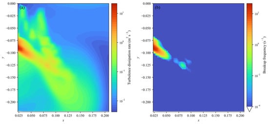
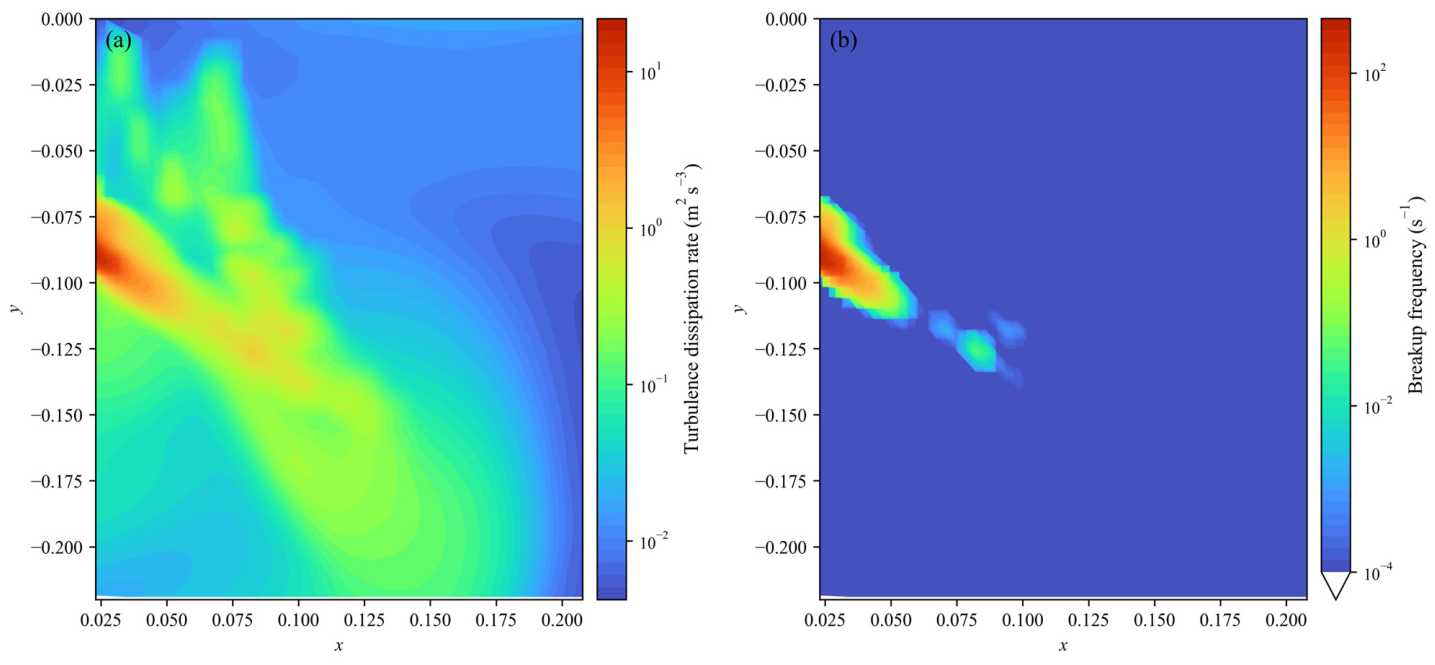
Figure 9 indicates that the turbulence field is highly nonuniform. The turbulence dissipation rate is highest near the SEN jet and along the main jet-transport path, where strong velocity gradients and gas–liquid momentum exchange are present. Based on a representative bubble diameter of 2 mm, the breakup-frequency map exhibits a similar but more localized high-value region, demonstrating that turbulent breakup mainly occurs in the intense dissipation zone rather than throughout the whole upper mold. Downstream from this region, the dissipation rate and breakup frequency rapidly decrease, so further bubble evolution is governed more by transport and by the force balance between drag and buoyancy. This explains why fine bubbles are generated mainly near the jet zone and then dispersed by the recirculating flow, while larger bubbles are more strongly affected by buoyancy during their upward migration.

Figure 9. Spatial distribution of turbulence dissipation rate and bubble breakup frequency in the analyzed mold region obtained using the M-type breakup model. (a) Turbulence dissipation rate. (b) Breakup frequency calculated for a representative bubble diameter of 2 mm. Both panels use logarithmic color scales, with warmer colors corresponding to higher values. Gas volume flow rate = 0.037 m³/h.

6. Conclusions

This study established an Euler–Lagrange model with bubble motion, collision coalescence, and turbulence-induced breakup to analyze bubble-size evolution and spatial distribution in a continuous casting mold. The revised conclusions are summarized as follows:

(1)

The model reproduces the main bubble-cloud morphology and bubble-size statistics observed in the water model experiment. Among the three daughter-size distribution assumptions, the M-type breakup distribution gives the best overall agreement with the experimental number-fraction distribution and median-diameter trend. For the median bubble diameter at different gas flow rates, the M-type model gives the lowest mean absolute error of 0.0349 mm, lower than the values for the U-type and N-type models. In contrast, the U-type model tends to generate too many fine bubbles, and the N-type model does not sufficiently represent the downstream dominance of small bubbles.

(2)

The bubble-size distribution shows a clear spatial dependence. Large bubbles with diameters greater than 2.5 mm account for about 4% of the total bubble number and are mainly concentrated near the SEN, whereas small bubbles with diameters of 1.0–1.5 mm account for about 60% and are widely distributed in the upper recirculation region. The median bubble diameter generally decreases from the SEN toward the narrow face, while increasing gas flow rate shifts the median diameter upward and widens the interquartile interval.

(3)

The mechanism analysis clarifies the relative roles of drag, buoyancy, and turbulence dissipation. In the high-velocity jet region, bubbles are mainly transported by liquid-phase drag and follow the mainstream flow. As the liquid velocity decreases downstream, buoyancy becomes more important, especially for larger bubbles. Turbulent breakup is concentrated near the SEN jet and along the high-dissipation path, so fine bubbles are mainly generated in localized turbulent regions and then dispersed by the recirculating flow.

The present model still has limitations. Although the water model preserves the main mold-scale flow similarity, direct bubble-scale similarity between water-air and steel-argon systems cannot be fully achieved because surface tension affects Weber-number-related collision criteria, bubble deformation, and the absolute turbulent breakup rate. In addition, bubbles are represented by equivalent diameters, while detailed interface deformation, slag-layer interaction, inclusion attachment, and solidification-front capture are not resolved. Future work should further validate the model under real steel casting conditions and examine different submerged entry nozzle configurations, including port angle, port area, port shape, and immersion depth, because nozzle geometry directly changes the jet structure, turbulence dissipation field, and local balance between drag and buoyancy.

References

- Yang, W.; Luo, Z.; Gu, Y.; Liu, Z.; Zou, Z. Simulation of bubbles behavior in steel continuous casting mold using an Euler-Lagrange framework with modified bubble coalescence and breakup models. Powder Technol. 2020, 361, 769–781. [Google Scholar] [CrossRef] [Scilit]
- Wu, Y.; Liu, Z.; Li, B.; Xiao, L.; Gan, Y. Numerical simulation of multi-size bubbly flow in a continuous casting mold using an inhomogeneous multiple size group model. Powder Technol. 2022, 402, 117368. [Google Scholar] [CrossRef] [Scilit]
- Javurek, M.; Wincor, R. Bubbly mold flow in continuous casting: Comparison of numerical flow simulations with water model measurements. Steel Res. Int. 2020, 91, 2000415. [Google Scholar] [CrossRef] [Scilit]
- Tian, Y.; Xu, L.; Qiu, S.; Zhu, R. Simulation of Spatial Distribution of Multi-Size Bubbles in a Slab Continuous-Casting Mold Water Model. Materials 2023, 16, 4666. [Google Scholar] [CrossRef] [Scilit]
- He, Z.; Cheng, Q.; Lu, H.; Zhong, Y.; Cheng, C.; Song, J.; Lei, Z. Numerical Simulation of Flow and Argon Bubble Distribution in a Continuous Casting Slab Mold under Different Argon Injection Modes. Metals 2023, 13, 2010. [Google Scholar] [CrossRef] [Scilit]
- Dinda, S.K.; Li, D.; Guerra, F.; Cathcart, C.; Barati, M. Sampling Strategy of Bubble Characteristics in a 1:2 Scale Curved Continuous Casting Mold: Parametric and Prediction Study. ISIJ Int. 2024, 64, 2031–2041. [Google Scholar] [CrossRef] [Scilit]
- Lai, Q.; Luo, Z.; Zhang, Y.; Zou, Z.; Li, H. Numerical Simulation of Bubble Flow in Continuous Casting Mold with Bubble Swarm Correction of Drag Coefficient. Metals 2025, 15, 952. [Google Scholar] [CrossRef] [Scilit]
- Xia, H.; Li, Q.; Chen, S.; Yang, J.; Fan, Z.; Xie, Y. Modeling of multiphase flow, bubble, and slag entrapment in slab continuous casting. Phys. Fluids 2025, 37, 053325. [Google Scholar] [CrossRef] [Scilit]
- Zhao, S.; Li, Z.; Zhu, Y.; Lyu, J. Mechanism analysis of surface black line and upwarping defects on low carbon hot-rolled plate. China Metall. 2021, 31, 7. [Google Scholar]
- Gass, R.; Knoepke, H.; Moscoe, J. Conversion of Ispat Inland’s No. 1 slab caster to vertical bending. In Proceedings of the ISSTech 2003 Conference Proceedings, Indianapolis, IN, USA, 27–30 April 2003; pp. 3–18. [Google Scholar]
- Rocabois, P.; Pontoire, J.-N.; Delville, V. Different slivers type observed in SOLLAC steel plants and improved practice to reduce surface defects on cold rolled sheet. In Proceedings of the ISSTech 2003 Conference Proceedings, Indianapolis, IN, USA, 27–30 April 2003; pp. 995–1006. [Google Scholar]
- Šolc, M.; Markulik, Š.; Małysa, T. The Influence of the Melting and Casting Parameters on the Surface Quality of Deep-Drawn Steel Coils. Sustainability 2025, 17, 1003. [Google Scholar] [CrossRef] [Scilit]
- Li, Y.; Liu, Z.; Xu, G.; Li, B. Effect of breakup and coalescence kernels on polydispersed bubbly flow in continuous casting mold. Int. J. Multiph. Flow 2024, 177, 104872. [Google Scholar] [CrossRef] [Scilit]
- Xu, T.; Deng, A.; Li, Y.; Wang, E. Numerical Simulation of Ar Bubbles Fragmentation-Polymerization and Trapping Behavior in Continuous Casting Mold. Acta Metall. Sin. 2025, 61, 1895–1910. [Google Scholar] [CrossRef]
- Lehr, F.; Millies, M.; Mewes, D. Bubble-Size distributions and flow fields in bubble columns. AIChE J. 2002, 48, 2426–2443. [Google Scholar] [CrossRef] [Scilit]
- Luo, H.; Svendsen, H.F. Theoretical model for drop and bubble breakup in turbulent dispersions. AIChE J. 1996, 42, 1225–1233. [Google Scholar] [CrossRef] [Scilit]
- Lee, C.H.; Erickson, L.E.; Glasgow, L.A. Dynamics of bubble size distribution in turbulent gas-liquid dispersions. Chem. Eng. Commun. 1987, 61, 181–195. [Google Scholar] [CrossRef] [Scilit]
- Chesters, A.K.; Hofman, G. Bubble coalescence in pure liquids. Appl. Sci. Res. 1982, 38, 353–361. [Google Scholar] [CrossRef] [Scilit]
- Wu, Y.; Liu, Z.; Li, B.; Gan, Y. Numerical simulation of multi-size bubbly flow in a continuous casting mold using population balance model. Powder Technol. 2022, 396, 224–240. [Google Scholar] [CrossRef] [Scilit]
- Liu, Z.Q.; Li, L.M.; Qi, F.S.; Li, B.K.; Jiang, M.F.; Tsukihashi, F. Population balance modeling of polydispersed bubbly flow in continuous-casting using multiple-size-group approach. Metall. Mater. Trans. B 2014, 46, 406–420. [Google Scholar] [CrossRef] [Scilit]
- Li, Y.; Liu, Z.; Yao, Y.; Li, B.; Xu, G. Effect of two-phase turbulent modalities and bubble-induced turbulence on polydispersed bubbly flow in continuous casting mold. Int. J. Multiph. Flow 2025, 184, 105104. [Google Scholar] [CrossRef] [Scilit]
- Liu, Z.; Li, Y.; Yao, Y.; Wang, N.; Li, S.; Li, B. Computational fluid dynamics simulation of polydispersed bubbly flow in continuous casting mold: Investigations on bubble-induced turbulence effect. Phys. Fluids 2025, 37, 085110. [Google Scholar] [CrossRef] [Scilit]
- Liu, Y.; Ersson, M.; Liu, H.; Jonsson, P.; Gan, Y. Comparison of Euler-Euler Approach and Euler-Lagrange Approach to Model Gas Injection in a Ladle. Steel Res. Int. 2019, 90, 1800494. [Google Scholar] [CrossRef] [Scilit]
- Cheng, C.; Lu, H.; Li, Y.; Qing, X.; Jin, Y. Mathematical Modeling of Flow and Heat Transfer Behavior of Liquid Slag in Continuous Casting Mold with Argon Blowing. ISIJ Int. 2019, 59, 1266–1275. [Google Scholar] [CrossRef] [Scilit]
- Jin, K.; Thomas, B.G.; Ruan, X.M. Modeling and measurements of multiphase flow and bubble entrapment in steel continuous casting. Metall. Mater. Trans. B 2015, 47, 548–565. [Google Scholar] [CrossRef] [Scilit]
- Zhang, T.; Luo, Z.G.; Zhou, H.; Ni, B.; Zou, Z.S. Analysis of two-phase flow and bubbles behavior in a continuous casting mold using a mathematical model considering the interaction of bubbles. ISIJ Int. 2016, 56, 116–125. [Google Scholar] [CrossRef] [Scilit]
- Lai, Q.R.; Luo, Z.G.; Hou, Q.F.; Zhang, T.; Wang, X.A.; Zou, Z.S. Numerical Study of Inclusion Removal in Steel Continuous Casting Mold Considering Interactions Between Bubbles and Inclusions. ISIJ Int. 2018, 58, 2062–2070. [Google Scholar] [CrossRef] [Scilit]
- Yang, W.; He, P.; Chang, L.; Li, T.; Bai, X.; Luo, Z.; Zhao, N.; Liu, Q. Numerical Analysis of Slag-Steel-Air Four-Phase Flow in Steel Continuous Casting Model Using CFD-DBM-VOF Model. Metals 2023, 13, 1943. [Google Scholar] [CrossRef] [Scilit]
- Yang, H.; Jin, B.-M.; Kim, H.; Seo, S.; Sim, S. A Practical 1D Approach for Real-Time Prediction of Argon Flow and Pressure in Continuous Casting of Steel. Metals 2025, 15, 978. [Google Scholar] [CrossRef] [Scilit]
- Olia, H.; Palmer, D.; Jebellat, E.; Thomas, B.G. Investigation of Multiphase Flow in Continuous-Casting Water Model with Measurements and Computational Modeling. Fluids 2025, 10, 113. [Google Scholar] [CrossRef] [Scilit]
- Ishii, M.; Zuber, N. Drag coefficient and relative velocity in bubbly, droplet or particulate flows. AIChE J. 1979, 25, 843–855. [Google Scholar] [CrossRef] [Scilit]
- Spelt, P.; Biesheuvel, A. On the motion of gas bubbles in homogeneous isotropic turbulence. J. Fluid Mech. 1997, 336, 221–244. [Google Scholar] [CrossRef] [Scilit]
- Roghair, I.; Van Sint Annaland, M.; Kuipers, H.J.A.M. Drag force and clustering in bubble swarms. AIChE J. 2013, 59, 1791–1800. [Google Scholar] [CrossRef] [Scilit]
- Zhang, D.; Deen, N.G.; Kuipers, J.A.M. Numerical simulation of the dynamic flow behavior in a bubble column: A study of closures for turbulence and interface forces. Chem. Eng. Sci. 2006, 61, 7593–7608. [Google Scholar] [CrossRef] [Scilit]
- Troshko, A.; Hassan, Y. A two-equation turbulence model of turbulent bubbly flows. Int. J. Multiph. Flow 2001, 27, 1965–2000. [Google Scholar] [CrossRef] [Scilit]
- Duineveld, P. Bouncing and coalescence of bubble pairs rising at high Reynolds number in pure water or aqueous surfactant solutions. Appl. Sci. Res. 1998, 58, 409–439. [Google Scholar] [CrossRef] [Scilit]
- Sungkorn, R.; Derksen, J.J.; Khinast, J.G. Euler-Lagrange modeling of a gas-liquid stirred reactor with consideration of bubble breakage and coalescence. AIChE J. 2012, 58, 1356–1370. [Google Scholar] [CrossRef] [Scilit]
Disclaimer/Publisher’s Note: The statements, opinions and data contained in all publications are solely those of the individual author(s) and contributor(s) and not of MDPI and/or the editor(s). MDPI and/or the editor(s) disclaim responsibility for any injury to people or property resulting from any ideas, methods, instructions or products referred to in the content. |
© 2026 by the authors. Licensee MDPI, Basel, Switzerland. This article is an open access article distributed under the terms and conditions of the Creative Commons Attribution (CC BY) license.