


Abstract
Chip-splitting can reduce cutting resistance, but its abrupt transition makes quantitative prediction difficult. This study proposes a catastrophe theory-informed framework for predicting the chip state and specific cutting force in the thread turning of 6061-T6 aluminum alloy. The framework combines a random forest classifier with a fully connected neural network and uses domain-adversarial training to introduce the fold geometry of a cusp catastrophe equilibrium surface as a regularizer. The experimental dataset comprises 1252 densely sampled equilibrium points from seven cutting force curves. Classification used a stratified 1001/251 train/test split, whereas regression held out Experiments 2, 4, and 6 (539 samples) and used the remaining 713 samples for training and validation. The random forest achieved 100.00% accuracy on the stratified test set. Across three initializations, the full regression model achieved MAPE = 1.74% ± 0.36%, R2 = 0.9815 ± 0.0020, maximum absolute percentage error = 4.47%, and normalized RMSE = 0.1315, which outperformed transfer learning, support vector regression, and the unconstrained FCN. The proposed framework shows that combining catastrophe theory geometry with machine learning can improve the prediction of chip-splitting states and specific cutting force in thread turning.
1. Introduction
In non-free cutting involving the simultaneous engagement of multiple cutting edges or a non-straight cutting edge, continuous variation in a cutting control parameter may cause a single chip to abruptly split into two separate chips. In this study, this discontinuous transition is referred to as a chip-splitting catastrophe [1]. The term “catastrophe” emphasizes the abrupt change in chip morphology induced by a continuous variation in the control parameter. Experimental observations reveal that the specific cutting force Kc drops abruptly by up to 64.68% [1] at the moment of bifurcation. This indicates that, under identical process conditions, the system can stably operate in at least two distinct Kc states with significantly different energy consumption levels. This behavior does not contradict determinism or experimental repeatability. Instead, it challenges the assumption that a continuously varied cutting input must produce a smooth, single-valued response: a deterministic process can still exhibit a discontinuous, path-dependent transition. Conversely, it opens a potential pathway for process energy saving. Once the underlying mechanisms are clarified, appropriate process measures could actively steer the system toward the lower Kc state.
Catastrophe theory [2] provides two primary approaches for modeling catastrophic phenomena: theoretical modeling and experimental modeling. These approaches yield mathematical models comprising potential functions, equilibrium surface equations, and bifurcation set equations. Modeling practices for cutting-induced catastrophes—including chip-splitting catastrophes—reveal a fundamental limitation. Models constructed solely on catastrophe theory exhibit relatively low prediction accuracy. This deficiency impedes their practical application in energy-saving strategies. Specific evidence supports this observation. Zhu et al. [3] developed a cusp catastrophe equilibrium surface equation for chip flow angle catastrophes using theoretical modeling. Their model showed a maximum prediction error of 19.47% for the critical depth of cut. Xu et al. [4] established a butterfly catastrophe bifurcation set equation for chip-splitting in the cylindrical turning of 6061-T6 aluminum alloy through experimental modeling. The prediction error for the critical depth of cut reached 34.54%. Similarly, You et al. [1] built a swallowtail catastrophe bifurcation set equation for chip-splitting catastrophes via experimental methods. Their model yielded a maximum prediction error of 50.44% for critical cutting thickness. Xu et al. [5] constructed a cusp catastrophe equilibrium surface equation for chip-splitting catastrophes using experimental data. Although their model achieved 100.0% accuracy in predicting chip-splitting occurrence, the maximum absolute prediction error for specific cutting force (Kc) remained as high as 22.07%. Such inaccuracy renders the model inadequate for guiding energy-saving applications of chip-splitting catastrophes.
The fundamental cause of these limitations lies in the qualitative nature of catastrophe theory itself [6,7,8,9]. Mathematical models derived from this theory are essentially analogy-based and qualitative [10,11]. They inherently lack quantitative predictive capability.
This intrinsic limitation has motivated researchers to explore a complementary fusion of machine learning and catastrophe theory. Machine learning provides strong nonlinear fitting capacity to enhance prediction accuracy. Catastrophe theory contributes geometric priors to constrain physical plausibility. Evidence supports this synergistic approach. Zheng et al. [12] developed a random forest (RF) classifier [13] for chip-splitting state prediction. It achieved 100.0% classification accuracy. This validates the superiority of data-driven methods in state discrimination tasks. Wang et al. [14] integrated transfer learning with catastrophe theory to model chip flow angle catastrophes. Their cusp catastrophe equilibrium surface equation predicted both chip flow angle and the critical depth of cut. Mean squared errors reached only 1.18% and 1.30%, respectively. This demonstrates the effectiveness of theoretical priors in improving model generalization. Collectively, these studies confirm that hybrid modeling—combining machine learning with catastrophe theory—offers significant technical advantages over pure catastrophe theory-based approaches for modeling catastrophic phenomena in machining processes.
Beyond hybrid catastrophe theory and machine learning studies, previous studies have investigated chip behavior and cutting force prediction in machining. Yılmaz et al. [15] reviewed chip-breaking mechanisms and control strategies in turning. Kouadri et al. [16] quantified chip segmentation in aluminum alloy machining and related segmentation intensity to cutting force fluctuations. Rezayi Khoshdarregi and Altintas [17] developed an experimentally validated mechanic model for chip geometry and cutting forces in multi-point thread turning, while Marani et al. [18] used a neuro-fuzzy model to predict cutting force in aluminum alloy turning. For aluminum alloy internal threading, Steininger et al. [19] examined process stability in tapping Al-Si alloys, and Korhonen et al. [20] investigated how diamond-coated tools affect tapping torque in 6082-T6 aluminum alloy. These studies addressed chip control, force or torque, stability, and tool effects, but they did not jointly model a split/unsplit transition and specific cutting force by using cusp catastrophe geometry as a learning constraint.
Machine learning techniques are particularly well suited for nonlinear problems. Decades of development have yielded numerous efficient algorithms. Domain-Adversarial Neural Networks (DANNs) [21] represent a prominent example. Prediction models for nonlinear phenomena—especially those exhibiting catastrophic behavior—built with DANNs typically demonstrate strong and accurate predictive performance. Fang et al. [22] constructed a building energy consumption prediction model based on Long Short-Term Memory–Domain-Adversarial Neural Networks (LSTM-DANN). This hybrid architecture effectively captured temporal dependencies while enhancing generalization across domains. These cases illustrate DANNs’ capability in modeling complex nonlinear systems with high fidelity.
To date, no studies have reported the use of Domain-Adversarial Neural Networks (DANNs) for predicting the magnitude of specific cutting force (Kc) in machining processes. Similarly, no hybrid modeling approaches combining machine learning with catastrophe theory have been developed for chip-splitting catastrophes. Such models would need to simultaneously predict two critical outputs: chip-splitting occurrence (binary state) and Kc magnitude (continuous value). This research gap motivates the present work.
The objective is to determine whether the fold geometry of a cusp catastrophe surface can improve two linked predictions under the present thread turning conditions: the split/unsplit chip state and the corresponding specific cutting force. The methodological contribution is a modular framework in which an RF handles classification, and a compact FCN handles regression, while theoretical geometry acts only as a training time distributional regularizer. This addresses the practical need for a quantitative, pre-machining comparison of candidate parameter combinations.
The framework has two components. First, an RF classifier uses cutting width and undeformed chip thickness to predict the binary chip state. Second, a 2–32–32–1 FCN predicts specific cutting force. During training, a DANN-based regularizer aligns experimental representations with features sampled from the folded cusp surface by combining the maximum mean discrepancy with an adversarial domain classification branch. During inference, the theoretical point cloud and DANN components are removed. This design tests whether a qualitative geometric prior can improve a quantitative predictor without increasing the deployed regressor.
2. Thread Turning Experiment Design and Data Acquisition
2.1. Experiment Design
A set of specially designed thread turning experiments was conducted on 6061-T6 aluminum alloy. The 6061-T6 aluminum alloy was selected because it is widely used in aerospace and mechanical manufacturing applications and exhibits good machinability, making it suitable for investigating nonlinear chip formation behaviors during cutting. The objective was to collect chip-splitting state data under varying cutting control parameters. Specifically, cutting width and cutting thickness were selected as control variables because they directly determine the geometric characteristics of the undeformed chip and strongly influence chip formation and transition behavior. The levels of these variables were determined according to the geometric characteristics of the conical workpiece and preliminary experimental observations, ensuring that the experimental range covered both unsplit and split chip states. Specifically, cutting width (aw) and cutting thickness (ac) were systematically varied. Corresponding equilibrium point coordinates (aw, ac, Kc) were measured experimentally. Both chip state (split/unsplit) and specific cutting force (Kc) were recorded for each parameter combination.
The variables were selected a priori from the controlled experimental design rather than identified by post hoc statistical screening. Workpiece material, tool geometry, cutting speed, and feed were held fixed. Cutting width (aD) varied continuously along the conical workpiece, whereas seven undeformed chip thickness levels (hD) were imposed through the depth-of-cut settings. These two quantities therefore served as independent process controls within the scope of the experiment. Specific cutting force (ks) was selected as the continuous state variable because it was measured synchronously and changed discontinuously when the observed chip morphology switched between unsplit and split states. The binary chip state label was retained separately for RF classification.
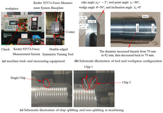
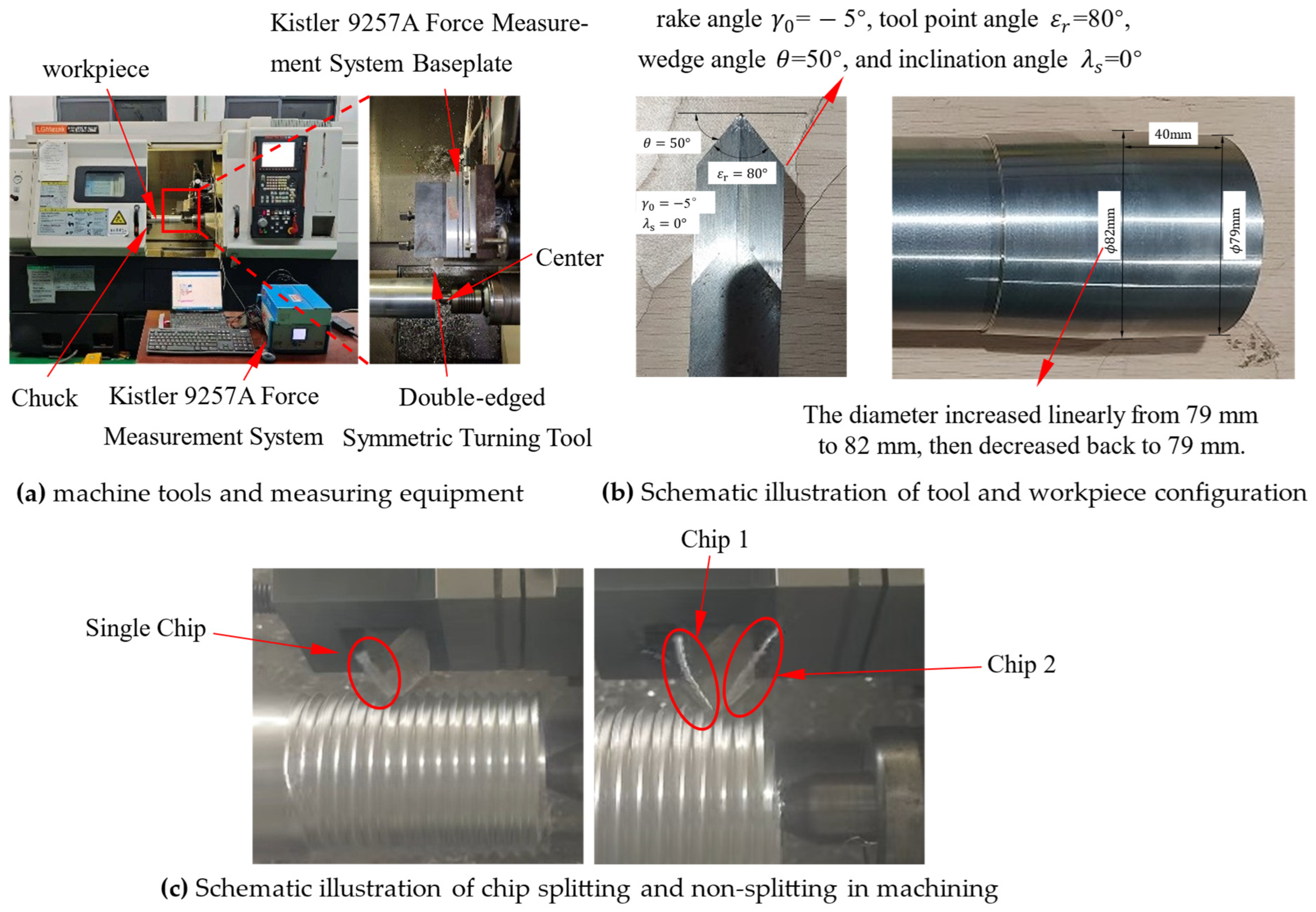
Experiments were conducted on a Mazak QTN200M horizontal turning center. The workpiece was a 6061-T6 aluminum alloy bar (Figure 1a). It was securely mounted between a three-jaw chuck and a live center. One end featured a symmetrical conical section. The diameter increased linearly from 79 mm to 82 mm, then decreased back to 79 mm. The other end was cylindrical with a thread pitch of p = 6 mm. A high-speed steel straight double-edged symmetrical turning tool was employed [23]. Its geometry parameters were: rake angle γ0= −5°, tool point angle εr = 80°, wedge angle θ = 50°, and inclination angle λs = 0° (Figure 1b). The tool holder was mounted horizontally and perpendicular to the workpiece rotational axis. The tool tip was aligned with the spindle centerline. Thread cutting was performed under dry conditions using longitudinal turning. The operation required three passes. The initial cutting speed was v= 5 m/min. The feed per revolution equaled the pitch: f = p = 6 mm/rev. The conical geometry caused the depth of cut (ap) to vary continuously during the first pass. The second and third passes used constant depths of cut. For experimental design, the second-pass depth of cut was set at seven levels: 0.05 mm, 0.10 mm, 0.15 mm, 0.20 mm, 0.25 mm, 0.30 mm, and 0.35 mm.
Figure 1.
The experimental setup, cutting tool, and chip-splitting phenomenon. (a) The experimental setup and measuring instruments configured for cutting force data acquisition. (b) The geometric configuration and relative position of the cutting tool and workpiece. (c) The morphological evolution of chips, illustrating the transition between chip-splitting and non-splitting states during the cutting process.
During the experiments, the dynamic main cutting force signal for the second pass (used here as an example to illustrate the proposed method; the procedure for the third pass is similar) was recorded using a Kistler 9257A three-component dynamometer (Kistler Instrumente AG, Winterthur, Switzerland). Simultaneously, the chip state during the second pass was captured using a slow-motion video recorded with an iPhone.
2.2. Acquisition of Chip States and Actual Equilibrium Point Measurements
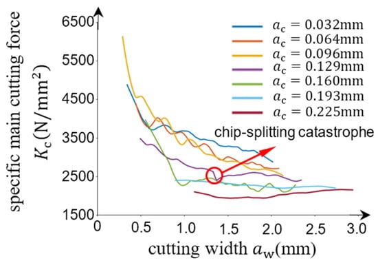
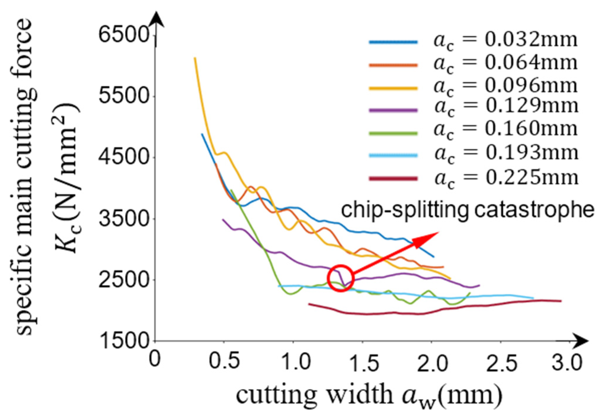
During data processing, the cutting width (aw) for the actual equilibrium point coordinates was determined based on the workpiece’s conical geometry. As the tool tip moved axially, aw varied continuously, first increasing and then decreasing. Its specific value at any given time could be calculated from the cutting time. The cutting thickness (ac) was derived from the geometric relationship among the cutting layer parameters, specifically ac = apcosθ, using the known ap. Since ap had seven levels, the calculated ac also had seven corresponding levels: 0.032 mm, 0.064 mm, 0.096 mm, 0.129 mm, 0.160 mm, 0.193 mm, and 0.225 mm. The specific cutting force (Kc) for the actual equilibrium point coordinates was calculated by processing the measured dynamic main cutting force signal. To minimize random error, the average value of the dynamic main cutting force over the entire tool path was used for this calculation. The resulting variation in the specific cutting force with cutting width is shown in Figure 2.
Figure 2.
Variation in the specific cutting force with cutting width.
Seven thread turning experiments produced seven specific cutting force curves. Equilibrium points were sampled at 0.01 mm intervals in cutting width, yielding 1252 samples in total.
As cutting width varied at a fixed undeformed chip thickness, the chip state could transition from unsplit to split, accompanied by a reduction in specific cutting force near the critical width. The cutting thickness levels, cutting width ranges, and observed chip states of the seven experiments are summarized in Table 1.
Table 1.
Data from turning 6061-T6 aluminum alloy conical bars.
2.3. Generation of Theoretical Equilibrium Point Data
Thread turning involves two varying control parameters. They are cutting width (aw) and cutting thickness (ac). Only one state parameter exists. It is the specific cutting force (Kc). According to catastrophe theory, a chip-splitting catastrophe belongs to the cusp catastrophe type.
The results from Experiment No. 4 in Table 1 reveal two critical control points for chip-splitting catastrophes. Their first coordinates are aw = 1.33 mm and aw = 1.34 mm, respectively. The difference between the two transition points is only 0.01 mm and may fall within experimental uncertainty; therefore, it is not regarded as quantitative evidence of hysteresis. Accordingly, the Maxwell convention [2] is adopted as a modeling assumption in the subsequent theoretical modeling, and the folded cusp catastrophe equilibrium geometry is used as the theoretical prior.
In catastrophe theory, a cusp catastrophe is a fundamental model. Its canonical equilibrium surface equation is expressed as follows:
4x3 + 2ux + v = 0
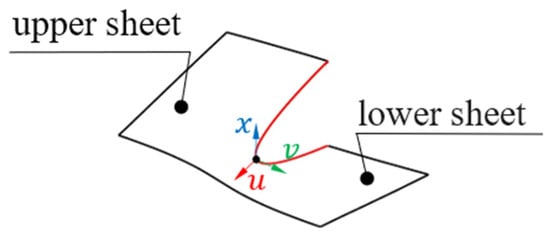
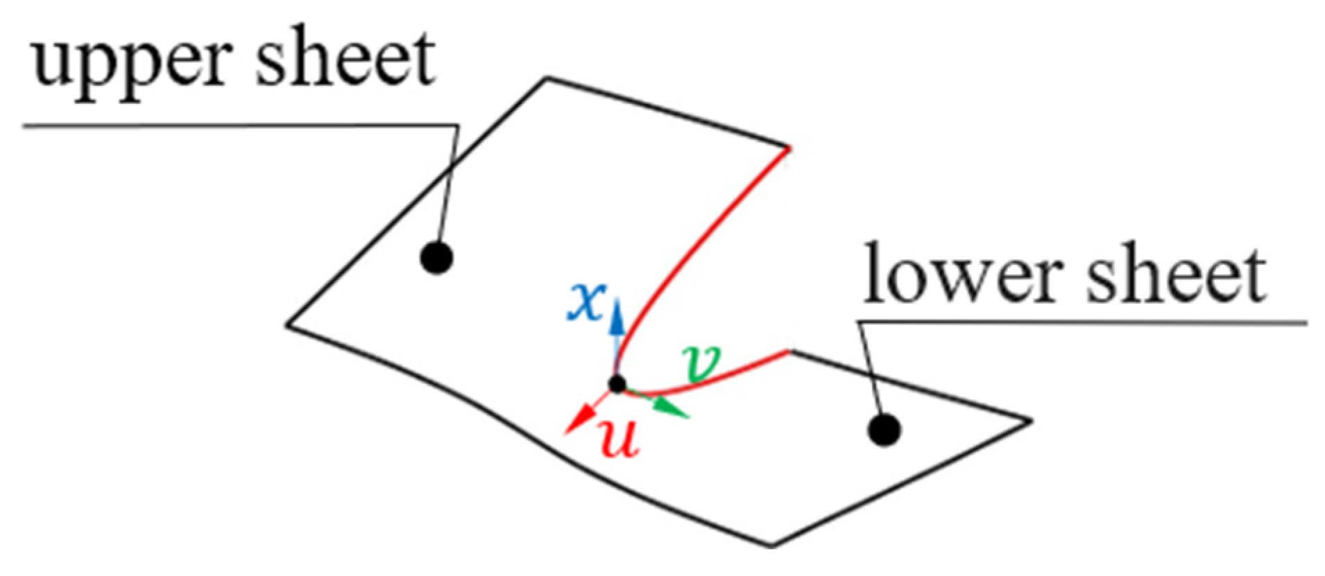
Here, x denotes the state parameter. u and v represent the control parameters.
The geometric shape of the cusp catastrophe regularized equilibrium surface can be plotted. This plot is based on the equilibrium surface equation and the Maxwell convention [2]. The result is shown in Figure 3. The red curve represents the bifurcation set. It delineates the critical boundary in control parameter space. When control parameters cross this boundary, the state parameter undergoes an abrupt discontinuous transition.
Figure 3.
Regularized equilibrium surface of cusp catastrophe.
The control grid contains 1001 values of u and 1001 values of v over [−5, 5] at a step of 0.01, giving 1001 × 1001 = 1,002,001 control parameter pairs. Under the Maxwell convention [2], the 500 pairs with v = 0 and u = −5.00, −4.99, …, −0.01 each contribute a second coexisting stable equilibrium state on the opposite sheet. The cusp point u = v = 0 is counted once. The resulting theoretical dataset therefore contains 1,002,001 + 500 = 1,002,501 equilibrium points. The source point cloud supplies folded geometry for training; it is not an additional experimental dataset.
3. Chip-Splitting State Prediction: RF Model
3.1. RF Model Architecture Design
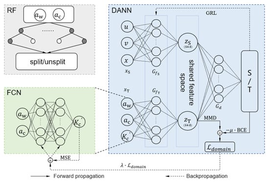
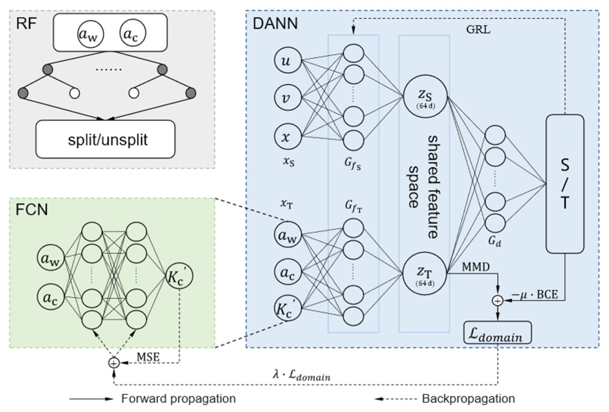
The chip-splitting state—split or unsplit—constitutes a binary classification problem. A random forest (RF) model was constructed for high-accuracy prediction. The input vector is x = (aw,ac), comprising cutting width and cutting thickness. The output is the chip state label, 0 for unsplit and 1 for split, as shown in Figure 4.
Figure 4.
Network architecture diagram. RF (upper left): classifies chip-splitting state using cutting width (aw) and thickness (ac). FCN (lower left): predicts specific cutting force () with 2 → 32 → 32 → 1 architecture trained by MSE. DANN (right): embeds catastrophe theory constraints through domain-adversarial training. Source encoder () and target encoder () map theoretical equilibrium points and experimental predictions into shared feature space (zS, zT). Domain classifier (Gd) distinguishes domains, with loss constrained by MMD and BCE. GRL (dashed arrow): reverses gradients during backpropagation for adversarial optimization.
The model comprises 100 decision trees: . Each tree independently votes to predict the chip state. The prediction of tree t is ht(x) = 0/1. Here, 0 denotes unsplit, and 1 denotes split. The final RF output follows the majority voting principle:
3.2. Dataset Splitting
The RF model for chip-splitting state prediction takes cutting width (aw) and cutting thickness (ac) as inputs. It was trained on the 1252 experimental samples obtained in Section 2.2.
To preserve the original proportion of split and unsplit samples in both training and testing sets, stratified sampling was employed. The dataset was partitioned into a training set (1001 samples) and a testing set (251 samples). The training–testing split ratio was 8:2.
3.3. RF Model Training and Validation
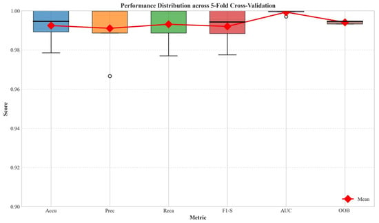
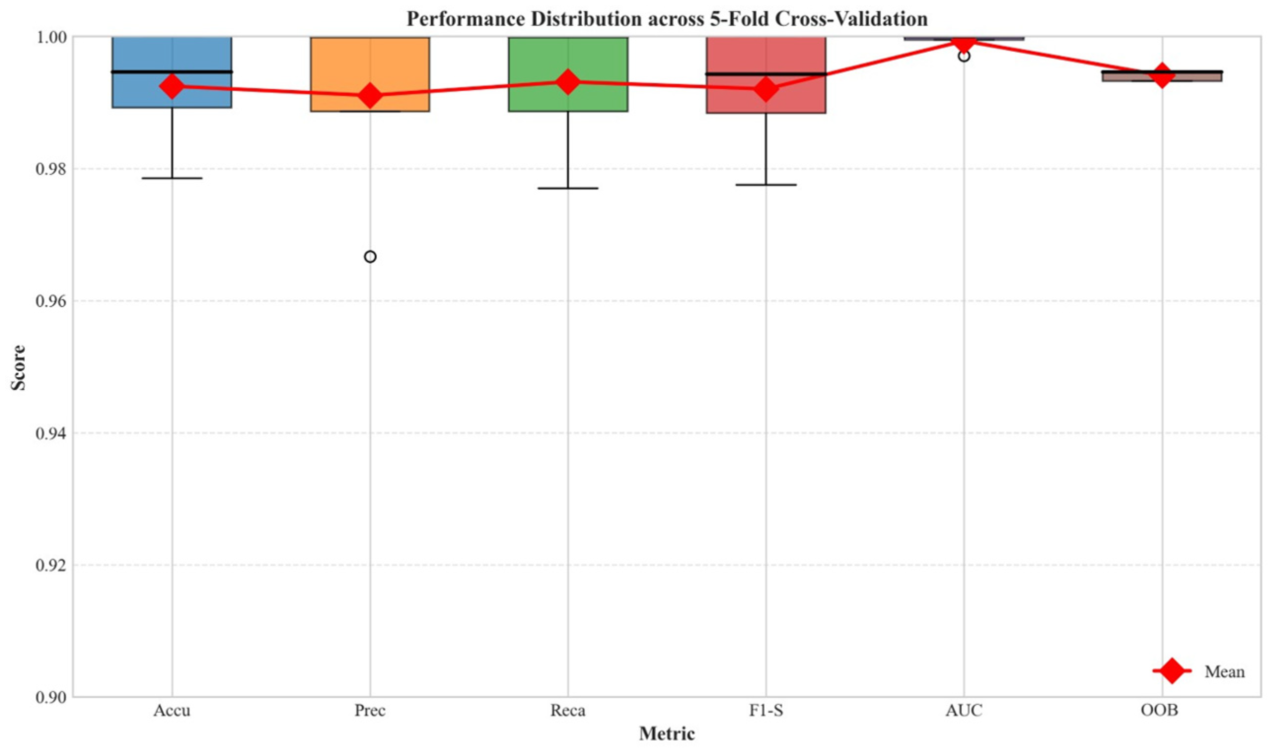
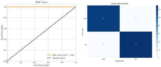
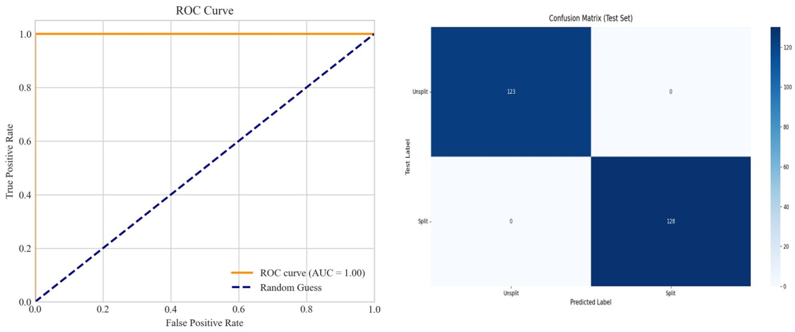
The RF used 100 decision trees and the Gini impurity criterion. Five-fold cross-validation was performed within the 1001-sample training set, with approximately 801 samples used for training and 200 for validation in each fold. Across three independent runs, the mean training, validation, and test accuracies were 99.20% ± 0.84%, 98.80% ± 1.30%, and 100.00% ± 0.00%, respectively. The variations in precision, recall, and F1-score during the 5-fold cross-validation process are shown in Figure 5. The mean values of these metrics were maintained above 0.99 with minimal fluctuations, confirming the model’s high consistency across different data subsets. On the stratified 251-sample test set, the RF produced no classification errors. The precision, recall, and F1-score were therefore 1.000 for each class and for the macro-, micro-, and weighted averages. The normalized confusion matrix contained unit diagonal elements and zero off-diagonal elements. The detailed confusion matrix and ROC curve for the independent test set are presented in Figure 6. The confusion matrix demonstrates perfect discrimination for both “split” and “unsplit” chip samples, with zero false positives and zero false negatives, and the AUC value reaches 1.0000.
Figure 5.
Evolution of accuracy, precision, recall, F1-score, AUC and OOB across 5-fold cross-validation iterations.
Figure 6.
Confusion matrix and ROC curve for independent test set.
4. Specific Cutting Force Prediction: Catastrophe Theory-Informed Regularized Neural Network
4.1. Fully Connected Neural Network Base Architecture Design
The prediction of specific cutting force (Kc) constitutes a continuous-value regression problem. A fully connected neural network (FCN) serves as the prediction backbone. Cutting width (aw) and cutting thickness (ac) are taken as inputs. The network outputs the predicted specific cutting force .
The network adopts a two-hidden-layer architecture. Each hidden layer contains 32 neurons. ReLU activation functions are employed in the hidden layers. The output layer uses linear activation. Network parameters are updated using the Adam optimizer. The loss function is initially defined as the mean squared error (MSE) between the predicted value and the measured value Kc:
4.2. Regularization Mechanism Constrained by Catastrophe Theory
To improve the prediction accuracy of the FCN in the catastrophe critical region, a Domain-Adversarial Neural Network (DANN) component is introduced. Geometric features revealed by cusp catastrophe theory—specifically, the folded structure of the equilibrium surface—are embedded as a regularization constraint during training. It should be emphasized that the DANN here does not serve conventional domain adaptation purposes. It is not employed for data transfer across domains (e.g., different machines under identical operating conditions). Instead, it functions as a theory-informed regularization technique. This approach converts qualitative geometric features from catastrophe theory into quantitative constraints learnable by neural networks.
The DANN component architecture is illustrated in Figure 4. It consists of the following elements:
Source domain input layer xS: Receives theoretical parameters (u,v,x) from the cusp catastrophe regularized equilibrium surface. This layer contains three nodes.
xS = (u,v,x)
Target domain input layer xT: Receives normalized process parameters and predicted values . This layer contains three nodes:
Source domain encoder (hidden layer parameters denoted as ): A single-layer ReLU network with 128 neurons. It maps xS to a 64-dimensional source domain feature representation zS:
Target domain encoder (hidden layer parameters denoted as ): A single-layer ReLU network with 128 neurons. It maps xT to a 64-dimensional target domain feature representation zT:
Domain classifier Gd (hidden layer parameters denoted as θd): A single-layer network with 32 neurons and sigmoid activation. It performs domain classification (source/target) on mini-batch samples z randomly drawn from zS and zT. The domain classification output is denoted as :
Gradient reversal layer (GRL): Reverses the sign of gradients during backpropagation. This mechanism enables adversarial training.
The source domain consists of 1,002,501 discrete equilibrium points (u,v,x) generated from the cusp catastrophe regularized equilibrium surface. These points inherently exhibit the folded structure of the equilibrium surface in feature space. They provide geometric prior knowledge of catastrophe phenomena for the model. The target domain is formed by actual cutting parameters (aw,ac) together with the real-time predicted specific cutting force output by the fully connected neural network. This domain fully characterizes the state evolution trajectory of the physical cutting process within the three-dimensional parameter space.
4.3. Loss Function Design and Implementation of Theoretical Constraints
The domain adversarial loss domain comprises two components. Together, they enforce regularization constraints that embed the geometric features of catastrophe theory.
The first component is the maximum mean discrepancy (MMD) [24]. It quantifies the distributional distance between source domain features zS and target domain features zT in the shared feature space. The objective is to minimize this discrepancy:
Here, ϕ(⋅) denotes the feature mapping in a Reproducing Kernel Hilbert Space (RKHS). The MMD term guides the target domain feature distribution toward the folded geometric structure inherent in the source domain. This alignment enables the network to learn a nonlinear mapping in the space that inherently exhibits folding characteristics prescribed by catastrophe theory.
The second component is binary cross-entropy (BCE). The domain classifier minimizes the standard, non-negative BCE loss to distinguish source domain from target domain features. When the BCE gradient is propagated from the classifier through the gradient reversal layer (GRL) to the encoders, the GRL multiplies that gradient by −μ. The encoders are therefore updated adversarially to reduce domain distinguishability, while the domain classifier itself continues to minimize BCE:
Here, yi denotes the ground-truth domain label (0 for source domain, 1 for target domain).
The classifier and the encoders consequently have opposing objectives. The reversed BCE gradient discourages domain-specific feature separation, whereas the MMD directly reduces the distributional discrepancy. The catastrophe-related geometric information originates from the theoretical source domain samples; BCE alone is not assumed to preserve that geometry.
The domain adversarial loss is defined as follows:
domain = MMD + μBCE
Here, μ is a prescribed GRL reversal coefficient or schedule, rather than a quantity computed by the GRL. It scales the reversed BCE gradient received by the encoders, while the MMD term is minimized directly.
The final total loss function is formulated as follows:
total = MSE + λdomain
Here, λ = 0.1 denotes the weighting coefficient for the domain-adversarial regularization and was selected by grid search. Equation (12) is written as a sum of non-negative scalar losses. In implementation, the domain classifier minimizes BCE normally, whereas the GRL reverses only the BCE gradient passed to the encoders; no additional explicit negative sign is applied to that encoder gradient.
Incorporating into the target domain input realizes the deep integration of theoretical priors with data-driven learning. During training, the network iteratively optimizes the mapping . This optimization progressively aligns the target domain feature distribution with the catastrophe-induced geometric structure embedded in the source domain. This dynamic alignment mechanism enables the model to simultaneously learn from empirical data distributions while actively conforming to the nonlinear mapping laws prescribed by catastrophe theory.
The regularization framework has three operational elements. First, theoretical equilibrium points provide a fixed source domain geometric prior. Second, the current FCN predictions form the target domain state coordinates, so the target representation changes as the regression model is updated. Third, the GRL applies the prescribed coefficient μ to reverse the BCE gradient reaching the encoders. The balance between prediction fitting and domain regularization is governed by λ and μ; the GRL changes gradient direction but does not compute these weights.
This synergistic mechanism—combining source domain prior guidance, target domain dynamic feedback, and GRL-based adaptive regulation—achieves two critical objectives. First, it enables the quantitative embedding of geometric features prescribed by catastrophe theory into the neural network’s learning process. Specifically, the MMD term aligns the target domain feature distribution with the folded source domain geometry, while the BCE term prevents degenerate distribution matching; their complementary roles are quantitatively supported by the ablation results in Section 5. Second, it preserves exceptional prediction stability throughout training and inference. This stability arises because the GRL-regulated constraint adaptively balances theoretical guidance against data-driven fitting, preventing the prior from dominating the learning process. Together, these properties provide a robust technical foundation for the high-accuracy prediction of chip-splitting catastrophe phenomena in thread turning processes.
4.4. Data Preprocessing and Dataset Partitioning
Cutting data were obtained from thread turning experiments on 6061-T6 aluminum alloy, as described in Section 2.2. The dataset comprises 1252 samples of (aw,ac,Kc). Theoretical equilibrium point data were generated by discretizing the cusp catastrophe regularized equilibrium surface, as detailed in Section 2.3. This dataset contains 1,002,501 samples of (u,v,x).
Subsequently, Z-score normalization was applied separately to the actual cutting data (aw,ac,Kc) and the theoretical data (u,v,x):
Here, μx and σx denote the mean and standard deviation of each variable computed independently within its respective dataset. Normalization was performed separately within the source and target domains. This independent processing prevents distributional shift caused by differences in physical units or scale.
To evaluate generalization to cutting thickness levels not used for model fitting, a non-random experiment-wise partition was adopted for the regression task. Experiment Nos. 2, 4, and 6, comprising 539 samples (43% of the total), formed the test set; the remaining 713 samples formed the training and validation pool. Grouping complete experimental curves prevents adjacent samples from the same curve from appearing in both the training and test sets. Within the 713-sample pool, however, five-fold cross-validation was sample-based. The holdout therefore assesses prediction at unseen thickness levels within the investigated parameter range rather than extrapolation beyond that range.
The target domain dataset partitioning for the DANN is identical to that of the FCN. The source domain data—comprising 1,002,501 theoretical equilibrium points—are not partitioned. All source domain samples are fully utilized to impose geometric constraints during training.
4.5. DANN Model Training and Validation
The catastrophe theory-informed regression model was trained using the Adam optimizer for a maximum of 100 epochs, with an early-stopping patience of 20 epochs. The Adam optimizer used a learning rate of 0.01 in all four model configurations. Model performance was evaluated using original-scale MAPE, R2, and normalized-target RMSE. The results are reported as the mean ± standard deviation over three random seeds (42, 123, and 456).
Within the 713-sample training/validation pool, five-fold cross-validation was performed using sample-based partitioning, with approximately 570 training samples and 143 validation samples per fold. The full model achieved training and validation MAPE values of 0.20% ± 0.03% and 0.23% ± 0.03%, respectively.
On the experiment-wise test set comprising 539 samples from Experiment Nos. 2, 4, and 6, the model achieved MAPE = 1.74% ± 0.36%, R2 = 0.9815 ± 0.0020, maximum absolute percentage error = 4.47%, and normalized RMSE = 0.1315. Approximate two-sided 95% Student’s t confidence intervals (n = 3; df = 2) were 0.85–2.63% for MAPE and 0.9765–0.9865 for R2.
5. Ablation Experiments and Mechanism Analysis
5.1. Ablation Experiment Design
Four controlled experiments were designed to systematically evaluate the contribution of each component within the catastrophe theory constraint framework, as summarized in Table 2.
Table 2.
Ablation study design.
All groups used the same network architecture, optimizer, learning rate configuration, maximum epoch count, early-stopping patience, data partitions, and three random seeds. Only the loss composition differed, making Table 3 a controlled comparison of the regularization terms under the present dataset.
Table 3.
Comparison of experimental results.
5.2. Prediction Performance Comparison
The prediction performance of the four models on the test set (539 samples) is presented in Table 3.
The results demonstrate the following:
- (1)
- The full model (Group D) achieved the lowest test MAPE and highest R2. Relative to the baseline FCN (Group A), its MAPE decreased from 5.60% ± 0.51% to 1.74% ± 0.36%, a 68.9% reduction, while R2 increased from 0.6767 ± 0.0487 to 0.9815 ± 0.0020. The smaller between-run standard deviation of R2 indicates lower sensitivity to the three evaluated random initializations.
- (2)
- The MMD-only model (Group B) reduced MAPE from 5.60% to 4.23% (24.5%) and increased R2 to 0.9132, indicating that direct distribution alignment contributes substantially to the improvement but is insufficient to match the combined model.
- (3)
- The BCE-only model (Group C) reduced MAPE from 5.60% to 5.08% (9.3%) and increased mean R2 to 0.7804, but its R2 standard deviation (0.1040) was the largest of the four groups. Thus, the adversarial branch alone provided limited and variable improvement under the evaluated initializations.
- (4)
- Combining the MMD and the adversarial BCE branch produced a larger improvement than either single-constraint variant and the smallest R2 variability. The ablation results support complementary roles for distribution alignment and adversarial feature learning under the present dataset.
5.3. Conclusions of Ablation Experiments
Through systematic ablation experiments and mechanism analysis, this section supports the following conclusions:
The full model reduced mean test MAPE from 5.60% ± 0.51% for the baseline FCN to 1.74% ± 0.36%, a 68.9% reduction. This supports the usefulness of the combined geometric regularizer under the evaluated conditions.
The MMD-only model improved more than the BCE-only model, whereas their combination produced the lowest MAPE and the smallest R2 variability. The result is consistent with complementary effects: the MMD directly reduces distribution discrepancy, and adversarial BCE discourages domain-specific separation. This interpretation remains statistical because the ablation data do not identify a unique physical coordinate transformation.
6. Comprehensive Performance Validation
To evaluate predictive performance, transfer learning (TL) and support vector machine (SVM) comparators were implemented for both tasks. Within each task, the proposed model and the comparators used the same input variables, samples, labels or targets, partition, and evaluation metrics. The classification and regression tasks used different task-specific partitions, as described in Section 3.2 and Section 4.4. Table 4 reports the resulting within-task comparisons.
Table 4.
Modeling accuracy across different models.
For chip state classification, all models used ac and aw as inputs and the 1252 experimental labels (0 = unsplit; 1 = split), with 1001 stratified training samples and 251 stratified test samples. For specific cutting force regression, all models used the same two inputs and ks as the target; Experiment Nos. 2, 4, and 6 (539 samples) were held out, and the remaining 713 samples were used for training and validation. The classification comparison therefore measures discrimination within the sampled parameter space, whereas the regression comparison measures generalization to unseen thickness levels within the investigated range.
For specific cutting force, the proposed, TL, and SVM models achieved training set MAPE values of 0.20% ± 0.03%, 1.76% ± 0.08%, and 3.72% ± 0.21%, with R2 values of 0.9999 ± 0.0000, 0.9918 ± 0.0029, and 0.9165 ± 0.0089. On the experiment-wise test set, their MAPE values were 1.74% ± 0.36%, 3.59% ± 0.56%, and 5.33% ± 0.20%, and their R2 values were 0.9815 ± 0.0020, 0.9186 ± 0.0203, and 0.7239 ± 0.0333. These same-partition results favor the proposed model within the investigated range.
For chip state classification, training accuracies were 99.20% ± 0.84%, 99.20% ± 1.01%, and 98.94% ± 1.00% for RF, TL, and SVM. Their stratified test accuracies were 100.00% ± 0.00%, 97.74% ± 0.46%, and 83.14% ± 4.98%. These values are directly comparable within the classification task because the inputs, labels, and split are shared. Because the split is random and sample-based, the result supports interpolation within the sampled parameter space.
7. Discussion
7.1. Methodological Advantages and Theoretical Contributions
The principal methodological contribution is to use a theoretical fold as a distributional training prior rather than as a stand-alone quantitative force law. The RF and FCN separate the classification and regression tasks, and the DANN components are used only while fitting the regressor. The 68.9% reduction in test MAPE relative to the same-capacity unconstrained FCN indicates that the regularizer is useful on the present held-out curves. This evidence supports the design choice, while independent experiments are still needed to establish broader physical generalization.
The source and target data are normalized independently before feature alignment. This allows the model to compare their dimensionless distributional geometry, but it does not identify a unique physical transformation between theoretical coordinates (u, v, x) and experimental coordinates (cutting width, undeformed chip thickness, and specific cutting force). Catastrophe theory supplies qualitative structural equivalence under the assumed one-state/two-control description; a quantitative global diffeomorphism would require a separately identified inverse-regularization model [25]. Accordingly, the theoretical surface is treated here as a shape prior, not as a unit-by-unit calibration of the machining process.
From an industrial perspective, the framework is intended as an offline tool for process planning. During inference, the theoretical point cloud, source/target encoders, domain classifier, MMD calculation, BCE branch, and GRL are not evaluated; only the 100-tree RF classifier and the 2–32–32–1 FCN regressor are required.
7.2. Analysis of Limitations and Applicability Boundaries
The scope of the reported performance is limited to the present 6061-T6 thread turning campaign. The 1252 samples come from seven correlated curves generated with one material, one tool geometry, one machine setup, and overlapping parameter ranges; the number of independent experimental units is seven. No second campaign, new tool, new material, or non-overlapping operating regime was available for external validation.
Material applicability: The model was evaluated only on 6061-T6 aluminum alloy. Chip formation differs across alloys and material classes, so retraining and independent testing are required before application elsewhere.
Tool and process dependence: The experiments used a fixed high-speed steel double-edged tool and fixed ancillary cutting conditions. A different tool, wear state, speed, lubrication condition, or machine can change chip evacuation and force. These variables were not tested.
Theoretical constraint boundary: A cusp is the lowest-codimension elementary form compatible with two controls and one state. The DANN alignment does not estimate the physical diffeomorphism between the theoretical and experimental spaces, and its success on the present data is not proof that the complete theoretical surface is quantitatively valid. Higher-codimension behavior would require additional controls and a redesigned prior.
8. Conclusions
This study developed a catastrophe theory-informed hybrid framework for split/unsplit classification and specific cutting force regression in the thread turning of 6061-T6 aluminum alloy. The method uses an RF classifier, a compact FCN regressor, and a training time distributional regularizer derived from the fold geometry of a cusp catastrophe surface.
The RF achieved 100.00% accuracy on a 251-sample stratified test set. Across three initializations, the full regression model achieved test MAPE = 1.74% ± 0.36% and R2 = 0.9815 ± 0.0020 on 539 samples from held-out experimental curves. Its mean MAPE was 68.9% lower than that of the unconstrained FCN, and the combined MMD–BCE regularizer outperformed either term alone under the same settings.
The current model is best viewed as an offline, within-range screening tool and as evidence that cusp geometry can be useful as a learning prior. Future work should prioritize independent repeat experiments, group-based validation at every model selection stage, broader tools and materials, quantitative chip shape measurements, and measured inference performance.
Author Contributions
Conceptualization, L.X.; methodology, L.X.; software, P.W.; validation, P.W.; formal analysis, S.Z. and M.X.; investigation, L.X., S.Z. and P.W.; resources, L.X.; data curation, L.X., P.W. and M.X.; writing—original draft preparation, L.X. and P.W.; writing—review and editing, P.W., M.X., S.Z. and B.Z.; visualization, B.Z., P.W. and S.Z.; supervision, L.X.; project administration, L.X.; funding acquisition, L.X. All authors have read and agreed to the published version of the manuscript.
Funding
This research was funded by the National Natural Science Foundation of China, grant number 52375432.
Data Availability Statement
The original contributions presented in this study are included in the article. Further inquiries can be directed to the corresponding author.
Acknowledgments
All experiments were conducted at the State Key Laboratory of Intelligent Manufacturing Equipment and Technology. The authors thank the laboratory staff for their experimental support. During the preparation of this manuscript, the authors used Qwen3.8-Max for language polishing and assistance in improving the wording and sentence structure of author-prepared text. The authors have reviewed and edited the output and take full responsibility for the content of this publication.
Conflicts of Interest
Author Peng Wu was employed by the company Dalian COSCO Shipping Heavy Industry Co., Ltd. The remaining authors declare that the research was conducted in the absence of any commercial or financial relationships that could be construed as a potential conflict of interest.
Abbreviations
The following abbreviations are used in this manuscript:
| BCE | Binary cross-entropy |
| DANN | Domain-adversarial neural network |
| FCN | Fully connected neural network |
| GRL | Gradient reversal layer |
| LSTM | Long short-term memory |
| MAPE | Mean absolute percentage error |
| MMD | Maximum mean discrepancy |
| MSE | Mean squared error |
| ReLU | Rectified linear unit |
| RF | Random forest |
| RKHS | Reproducing kernel Hilbert space |
| R2 | Coefficient of determination |
| SVM | Support vector machine |
| TL | Transfer learning |
References
- You, Q.; Xu, M.; Zhu, B.; Xiong, L.; Yin, K. Experimental Modeling of the Bifurcation Set Equation of the Chip-Splitting Catastrophe in Symmetrical Straight Double-Edged Cutting. Metals 2022, 12, 878. [Google Scholar] [CrossRef] [Scilit]
- Saunders, P.T. An Introduction to Catastrophe Theory; Cambridge University Press: Cambridge, UK, 1980; ISBN 978-0-521-23042-1. [Google Scholar]
- Zhu, B.; Xiao, Y.M.H.; Wan, X.; Xiong, L. Theoretical Modeling and Experimental Verification of Chip Flow Angle Catastrophe in Double-Edged Cutting Considering Non-Linear Effects. Int. J. Mech. Sci. 2020, 172, 105394. [Google Scholar] [CrossRef] [Scilit]
- Xu, M.; Xiong, L.; Cheng, D.; Zhang, S. Experimental Establishment of Butterfly-Type Bifurcation Set Equation for Chip-Splitting Catastrophe in Cylindrical Turning; American Society of Mechanical Engineers Digital Collection, 23 January 2025; American Society of Mechanical Engineers: New York, NY, USA, 2025. [Google Scholar]
- Xu, M.; Xiong, L.; Zhang, S. The Determination of the State Variable for Chip-Splitting Catastrophe and the Experimental Establishment of Cusp-Type Equilibrium Surface Equation. Nonlinear Dyn. 2025, 113, 27171–27195. [Google Scholar] [CrossRef] [Scilit]
- Boutot, A. Catastrophe Theory and Its Critics. Synthese 1993, 96, 167–200. [Google Scholar] [CrossRef] [Scilit]
- Kolata, G.B. Catastrophe Theory: The Emperor Has No Clothes. Science 1977, 196, 287–351. [Google Scholar] [CrossRef] [Scilit] [PubMed]
- Zahler, R.S.; Sussmann, H.J. Claims and Accomplishments of Applied Catastrophe Theory. Nature 1977, 269, 759–763. [Google Scholar] [CrossRef] [Scilit]
- Stewart, I. In Support of Catastrophe Theory. Nature 1977, 270, 382. [Google Scholar] [CrossRef] [Scilit][Green Version]
- Zeeman, E.C.; Hall, C.S.; Harrison, P.J.; Marriage, G.H.; Shapland, P.H. A Model for Institutional Disturbances. Br. J. Math. Stat. Psychol. 1976, 29, 66–80. [Google Scholar] [CrossRef] [Scilit] [PubMed]
- Abrams, J.H.; Barke, R.A.; Cerra, F.B. Quantitative Evaluation of Clinical Course in Surgical ICU Patients: The Data Conform to Catastrophe Theory. J. Trauma 1984, 24, 1028–1037. [Google Scholar] [CrossRef] [Scilit] [PubMed]
- Zheng, L.; Xiong, L.; Xu, M.; Yin, K. Chip Bifurcation Machine Learning Forecasting Model Based on Experimental Data and Random Forest Algorithm. In Proceedings of the 2022 8th International Conference on Mechanical Engineering and Automation Science (ICMEAS), Virtual, 15 October 2022; pp. 207–213. [Google Scholar]
- Breiman, L. Random Forests. Mach. Learn. 2001, 45, 5–32. [Google Scholar] [CrossRef] [Scilit]
- Wang, Y.; Xiong, L.; Zhang, S.; Zhu, B. Experimental Modeling of Equilibrium Surface for Chip Flow Angle Catastrophe Based on Transfer Learning and Catastrophe Theory. CIRP J. Manuf. Sci. Technol. 2025, 59, 76–82. [Google Scholar] [CrossRef] [Scilit]
- Yılmaz, B.; Karabulut, Ş.; Güllü, A. A Review of the Chip Breaking Methods for Continuous Chips in Turning. J. Manuf. Process. 2020, 49, 50–69. [Google Scholar] [CrossRef] [Scilit]
- Kouadri, S.; Necib, K.; Atlati, S.; Haddag, B.; Nouari, M. Quantification of the Chip Segmentation in Metal Machining: Application to Machining the Aeronautical Aluminium Alloy AA2024-T351 with Cemented Carbide Tools WC-Co. Int. J. Mach. Tools Manuf. 2013, 64, 102–113. [Google Scholar] [CrossRef] [Scilit]
- Rezayi Khoshdarregi, M.; Altintas, Y. Generalized Modeling of Chip Geometry and Cutting Forces in Multi-Point Thread Turning. Int. J. Mach. Tools Manuf. 2015, 98, 21–32. [Google Scholar] [CrossRef] [Scilit]
- Marani, M.; Zeinali, M.; Farahany, S.; Mechefske, C.K. Neuro-Fuzzy Based Predictive Model for Cutting Force in CNC Turning Process of Al–Si–Cu Cast Alloy Using Modifier Elements. SN Appl. Sci. 2021, 3, 72. [Google Scholar] [CrossRef] [Scilit]
- Steininger, A.; Siller, A.; Bleicher, F. Investigations Regarding Process Stability Aspects in Thread Tapping Al-Si Alloys. Procedia Eng. 2015, 100, 1124–1132. [Google Scholar] [CrossRef] [Scilit]
- Korhonen, H.; Koistinen, A.; Lappalainen, R. Improvements in the Thread Cutting Torque for a 6082-T6 Aluminum-Based Alloy with Tapping Tools Utilizing Diamond Coating. Mach. Sci. Technol. 2018, 22, 696–728. [Google Scholar] [CrossRef] [Scilit]
- Ganin, Y.; Ustinova, E.; Ajakan, H.; Germain, P.; Larochelle, H.; Laviolette, F.; Marchand, M.; Lempitsky, V. Domain-Adversarial Training of Neural Networks. J. Mach. Learn. Res. 2016, 17, 1–35. [Google Scholar]
- Fang, X.; Gong, G.; Chun, L.; Li, W.; Peng, P. A Transfer Learning Method for Building Energy Prediction Using Long Short Term Memory and Domain Adversarial Neural Network. In Proceedings of the Applied Energy Symposium 2020: Low Carbon Cities and Urban Energy Systems (CUE2020), Virtual, 10–17 October 2020. [Google Scholar]
- Wang, Y.; Qian, C.; Kong, L.; Zhou, Q.; Gong, J. Design Optimization for the Thin-Walled Joint Thread of a Coring Tool Used for Deep Boreholes. Appl. Sci. 2020, 10, 2669. [Google Scholar] [CrossRef] [Scilit]
- Gretton, A.; Borgwardt, K.M.; Rasch, M.; Schölkopf, B.; Smola, A.J. A Kernel Method for the Two-Sample-Problem. In Advances in Neural Information Processing Systems 19; Schölkopf, B., Platt, J., Hofmann, T., Eds.; The MIT Press: Cambridge, MA, USA, 2007; pp. 513–520. ISBN 978-0-262-25691-9. [Google Scholar]
- Zhang, S.; Xiong, L.; Xu, M. Precise Regularization Method of Cusp-Type Catastrophe Mathematical Model Based on Global Diffeomorphism. J. Comput. Appl. Math. 2026, 476, 117084. [Google Scholar] [CrossRef] [Scilit]

Disclaimer/Publisher’s Note: The statements, opinions and data contained in all publications are solely those of the individual author(s) and contributor(s) and not of MDPI and/or the editor(s). MDPI and/or the editor(s) disclaim responsibility for any injury to people or property resulting from any ideas, methods, instructions or products referred to in the content. |
© 2026 by the authors. Licensee MDPI, Basel, Switzerland. This article is an open access article distributed under the terms and conditions of the Creative Commons Attribution (CC BY) license.