Fatigue Behavior and 3D Defect Analysis of 10CrNi3MoV Steel Multi-Pass Welded Joints

Abstract

Multi-pass welded joints of 10CrNi3MoV high-strength low-alloy (HSLA) steel were systematically investigated for high-cycle fatigue (HCF) behavior using microstructural characterization, mechanical behavior, and inherent defect analysis. Gas metal arc welding (GMAW; G1 and G2) and submerged arc welding (SAW; S1 and S2) were performed under two welding conditions each. The welded joints exhibit distinct microstructure and hardness across the fusion zone, coarse-grained heat-affected zone, fine-grained heat-affected zone, and base metal, while maintaining similar tensile strength (684.97 MPa–698.6 MPa). HCF behavior was evaluated at a stress ratio and stress frequency of 0.1 and 120 Hz, respectively. S–N curve was plotted with coefficients of determination values from 0.929 to 0.983. X-ray computed tomography revealed varied internal porosity and inclusions. Paired-case analysis at a maximum stress (σ_max) of 168 MPa and 300 MPa demonstrated a strong relationship between defect volume fraction and HCF life. Particularly, the 428-fold increase in porosity volume fraction reduced fatigue life from run-out (>10⁷ cycles) to failure after 773,100 cycles in S1. These findings demonstrate a critical influence of internal weld defects on the HCF life of 10CrNi3MoV welded joints, contributing to improved fatigue-life assessment and providing a basis for future research on fatigue-life assessment.

1. Introduction

High-strength low-alloy (HSLA) steel has become one of the most prominent classes of steel, as it provides better mechanical properties than conventional carbon steel. Currently, HSLA steels are widely joined through typical welding technologies to fabricate large vessel structures, bridges, and engineering components [1]. However, welded joints generally exhibit weak mechanical strength due to the metallurgical changes that occur during the welding process [2,3]. In particular, weld toes are stress concentration zones, which adversely affect component durability, making them particularly susceptible to fatigue-crack initiation after prolonged cyclic loads [4]. Accordingly, the fatigue performance of welded joints depends on the welding process, resultant microstructural gradients and the magnitude of internal defects [5].

Among different classes of HSLA steel, 10CrNi3MoV HSLA steel is a popular structural material in the shipbuilding industry, due to its high strength, good toughness, and excellent weldability [6]. Previous studies on 10CrNi3MoV HSLA steel have reported several aspects of 10CrNi3MoV HSLA steel fatigue behavior and its welded joints. The strain-controlled low-cycle fatigue (LCF) response of 10CrNi3MoV and undermatched welds was investigated. As a result, distinct cyclic deformation and crack initiation characteristics were observed in undermatched weld metal compared to the 10CrNi3MoV base alloy [7]. Strain-controlled fatigue tests were conducted over a strain amplitude range of 0.2–1.2%, and the cyclic softening behavior was mainly observed during the initial 5–15% of fatigue life. Further, HCF behavior of load-carrying cruciform welded joints was investigated considering strength mismatch and joint geometry [8]. Studying fatigue fracture mechanics on 10CrNi3MoV welded joints further reaffirmed the effects of the strength mismatch and initial crack geometry on fatigue crack growth [1,9,10]. More recently, the fatigue-crack propagation behavior of 10CrNi3MoV welded joints has also been examined under low-temperature conditions [11]. Collectively, the studies discussed above provide a basis for a detailed understanding of fatigue and crack propagation behavior of 10CrNi3MoV welded joints.

However, the studies on the evaluation of the mechanical behavior of 10CrNi3MoV welded joints were largely concentrated on cyclic deformation, crack-growth resistance, strength mismatch, geometric stress concentration, and fracture-mechanics parameters. They do not provide a systematic three-dimensional quantification of the inherent weld defect population and its connection with experimentally measured HCF life. This distinction is important because microscale defects in welded structures, such as porosity, inclusions, and undercuts, develop stress concentration zones that promote premature crack initiation, thereby accelerating crack growth and causing premature structural failure [12,13]. Evidence from other welded alloy systems supports this defect-controlled mechanism. For example, defect-induced fatigue crack initiation has been associated with localized deformation and microstructural heterogeneity in IN617B superalloy [12]. While studies on EBW TC17 titanium alloy welded joints indicate that pore size and location have a significant influence on crack initiation and fatigue life [14,15]. These studies establish the association between welded joint defects and alloy fatigue behavior. However, this scientific conclusion cannot be directly extrapolated to 10CrNi3MoV because of differences in alloy chemistry, microstructure, and welded joint metallurgy.

Nevertheless, experimental evidence from marine structural steels provides a more relevant basis for evaluating the role of weld defects in fatigue behavior. X-ray computed tomography (XCT) enables high-resolution three-dimensional characterization of defect size, morphology, spatial location, and distribution. It has been employed to characterize defects in defective AH36 welded joints used in ship structures, to quantify cumulative defect volume and maximum defect size. The reported fatigue strength was 64.7 MPa for defective joints compared with 94.7 MPa for joints without significant defects, while the predicted fatigue strength of imperfect joints ranged from 80 to 131 MPa compared with 107–137 MPa for perfect joints [16]. The results indicated that fatigue strength was reduced with an increase in defect severity, suggesting a strong correlation between three-dimensional defect characteristics and fatigue behavior. Similarly, very-high-cycle fatigue investigations of EH36 welded joints have shown that internal defects in the fusion region can act as fatigue-crack initiation sites and are linked to fatigue life. Fatigue fracture in EH36 welded joints was observed even in the range of 10⁸–10¹⁰ cycles, with fatigue cracks mainly initiating from internal defects in the fusion region [17]. The above studies demonstrate the significance of defect characterization for marine welded steels, but AH36 and EH36 differ substantially from 10CrNi3MoV in chemical composition, phase constituents and mechanical response. Therefore, it is important to determine the influence of three-dimensional defect populations on HCF performance in 10CrNi3MoV welded joints. However, there exists limited understanding of the effects of three-dimensional defect populations obtained by XCT on HCF, crack initiation, and fatigue life of 10CrNi3MoV HSLA steel welded joints.

In the present study, four 10CrNi3MoV multipass welded joints produced under different processing conditions are systematically investigated through microstructural characterization, tensile testing and HCF S–N testing, followed by three-dimensional XCT characterization of internal defects. Particular emphasis is placed on examining the association between XCT-resolved pore characteristics and HCF life through paired-case analysis. This integrated approach linking processing, microstructure, defects, and fatigue complements previous 10CrNi3MoV studies based on cyclic deformation, crack growth, and fracture mechanics, while providing a quantitative assessment of defect-dominated HCF behavior in this marine HSLA steel.

2. Experimental Procedures

2.1. Material and Welding Processes

The 10CrNi3MoV steel plates, 10 mm in thickness, were purchased from Anshan Iron and Steel Group Co., Ltd. (Anshan, China) in the quenched-and-tempered condition in accordance with the GJB 1663A-2018 standard [18]. The nominal and standard chemical compositions of the steel are presented in Table 1. The standard mechanical properties 10CrNi3MoV steel are given in Table 2 for reference. The plates were subsequently butt-welded using gas metal arc welding (GMAW) and submerged arc welding (SAW) techniques. Each of these welding processes is carried out at two different inter-pass temperatures and heat input conditions, resulting in a total of four weld specimens, designated as G1, G2, S1, S2. Specimens G1 and G2 are GMAW with linear energy 11.4 and 12.7 kJ·cm⁻¹, whereas S1 and S2 are SAW with linear energy of 19.1 and 34.6 kJ·cm^−1, respectively. The inter-pass temperatures of G1 and G2 are 120~140 °C and 50~70 °C, whereas the inter-pass temperatures of S1 and S2 are 90~110 °C.

Table 1. Nominal and standard chemical composition of 10CrNi3MoV high-strength low-alloy (HSLA) steel (wt %).

Element	C	S	P	Si	Mn	Ni	Cr	Mo	V	O	N	Fe
(wt.%)	0.072	<0.0010	0.0097	0.262	0.428	2.79	1.04	0.225	0.054	0.0013	0.0021	balance
GJB 1663A-2018 [18]	0.06–0.11	<0.01	<0.015	0.17–0.37	0.30–0.60	2.60–3.00	0.90–1.20	0.20–0.27	0.04–0.10	-	-	balance

Table 2. Standard 10CrNi3MoV HSLA steel yield strength, ultimate tensile strength, and elongation according to GJB 1663A-2018 [18].

Yield Strength (MPa)	Tensile Strength (MPa)	Elongation (%)
590–730	>655	>16

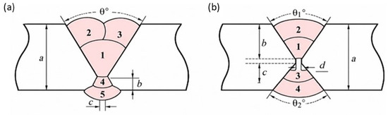
The GMAW joints (G1 and G2) were produced using an X-groove configuration with a four-layer welding sequence. A 1.2 mm diameter filler wire classified as G 69A 5 N1M3 N according to GB/T 39281-2020 [19] was used. The shielding gas consisted of 80% Ar and 20% CO₂ and was supplied at a flow rate of 15–20 L min⁻¹. The SAW joints (S1 and S2) were produced using a V-shaped groove configuration with a five-layer welding sequence. The SAW consumable combination was classified as S 69A 5 FB SU34 H5 according to GB/T 36034-2018 [20] with wire diameters of 3.0 mm for S1 and 4.0 mm for S2. Direct current reverse polarity was employed for all welding conditions. The detailed welding parameters are summarized in Table 3, and the groove geometries and welding-layer sequences are illustrated in Figure 1.

Table 3. Welding process parameters for the four joint configurations.

Specimen	Welding Method	Current (A)	Voltage (V)	Welding Speed (cm·min−1)	Linear Energy (kJ·cm−1)	Inter-Pass Temperature (°C)
G1	Gas-shielded welding	210 to 230	24 to 28	25 to 35	11.4	120 to 140
G2	Gas-shielded welding	220 to 240	28 to 32	30 to 35	12.7	50 to 70
S1	Submerged arc welding	350 to 400	28 to 32	38 to 42	19.1	90 to 110
S2	Submerged arc welding	600 to 650	28 to 32	30 to 35	34.6	90 to 110

Figure 1. Schematic illustration of the groove geometries and welding-layer sequences: (a) V-shaped groove and five-layer sequence for SAW joints; (b) X-shaped groove and four-layer sequence for GMAW joints. For the Y-type groove, a represents the plate thickness, b denotes the root dimension, and θ is the groove angle. For the X-type groove, a represents the plate thickness, b denotes the root dimension, c is the root opening at the central joint region, and d represents the corresponding dimension on the opposite side of the central joint region. The angles θ1 and θ2 represent the upper and lower groove angles, respectively. The numbers shown within the weld region indicate the weld layer (pass) sequence.

For the V-shaped groove, the plate thickness was 10 mm, the root dimension was 4 mm, and the groove angle was 60°. For the X-shaped groove, the plate thickness was 10 mm, with the corresponding groove angles of 60° and 90°.

2.2. Microstructural Characterization

2.2.1. Metallography Sample Preparation

As-received, mechanically deformed welded joints of G1, G2, S1, and S2 were cut in cross-section, ground using P2000 SiC paper (Shaoxing Ziyuan Polishing Co., Ltd., Shaoxing, China), polished with diamond suspension (1 μm), and finally etched with 4% nital solution.

2.2.2. Elemental and Microstructural Analyses

The elemental composition of as-received tempered 10CrNi3MoV HSLA steel was analyzed using a Hydrogen–Oxygen Gas Analyzer (LECO, ONH836, LECO Corporation, St. Joseph, MI, USA), Inductively Coupled Plasma Optical Emission Spectrometer (Agilent 5110SVDV) (Agilent Technologies, Mulgrave, Australia), and Carbon–Sulfur Analyzer (ELTRA GmbH) (Haan, Germany).

Optical microscopy (OM; ZEISS AXIO Vert.A1) (Jena, Germany) was used to examine the morphology of as-received G1, G2, S1, and S2 welded specimens. The fracture surfaces of the tensile- and fatigue-tested specimens were characterized using a S-4800 scanning electron microscope (SEM) (Hitachi High-Tech Corporation, Tokyo, Japan) coupled with energy-dispersive X-ray spectroscopy (EDS; OXFORD ULTIM MAX 40) (Oxford Instruments, Abingdon, UK).

2.3. Mechanical Testing

2.3.1. Vickers Microhardness Testing

Vickers microhardness measurements were performed using an HVST-1000C micro-Vickers hardness testing system (Shanghai Zhongyan Instrument Manufacturing Co., Ltd., Shanghai, China) in accordance with GB/T 4340.1-2024 [21]. A test load of 0.5 kgf (HV0.5, approximately 4.90 N) was applied with a dwell time of 15 s. Measurements were conducted along a transverse path across the welded joint, covering the fusion zone, heat-affected zone (HAZ), and base metal. The indentation spacing was 1.0 mm in the fusion zone and base metal, whereas a spacing of 0.3 mm was used in the HAZ to resolve local hardness variations across the microstructural gradient. Three valid indentations within each corresponding region were included in the calculation of the mean hardness and standard deviation.

2.3.2. Tensile Testing

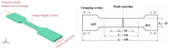
Specimens from all four welded joints G1, G2, S1 and S2 were prepared for room-temperature tensile testing in accordance with GB/T 228.1-2021 [22] (equivalent to ISO 6892-1 [23]). Accordingly, specimens 10 mm thick, 25 mm wide, and 240 mm in length with the weld seam located at the center of the parallel section, as shown in Figure 2, were machined. Three specimens from each weld condition were stretched vertically on a universal testing machine model INSTRON5985 (Instron, Norwood, MA, USA) at a crosshead speed of 2 mm·min⁻¹. Subsequent engineering stress–strain curves were recorded; 0.2% offset yield strength, ultimate tensile strength (UTS), elastic modulus, and strain to fracture were determined.

Figure 2. Tensile specimen model and schematic with dimensions in millimeters (mm).

2.3.3. High-Cycle Fatigue Testing

Fatigue tests were conducted on specimens with widths around 15.8–16.0 mm and thicknesses of 9.9–10.2 mm from the G1, G2, S1, and S2 welded joints in accordance with GB/T 3075-2021 [24]. The specimens were subjected to axial tension–tension fatigue loading using GPS-200 (Sinotest Equipment Co., Ltd., Changchun, China) and QBG-100 (Changchun Qianbang Testing Equipment Co., Ltd., Changchun, China) high-frequency fatigue testing machines. A sinusoidal waveform was applied at a frequency of 120 Hz and a stress ratio ($R={\sigma }_{min}/{\sigma }_{max})=0.1$. The maximum applied stress, ${\sigma }_{\mathrm{m}\mathrm{a}\mathrm{x}}$ ranged from 59 to 490 MPa. Specimens that survived ${10}^7$ cycles without fracture were classified as run-outs. In this study, specimens surviving the termination criterion of ${10}^7$ cycles without failure were classified as run-outs. Since these observations are right-censored, they were not treated as failures at exactly ${10}^7$ cycles and were therefore excluded from the ordinary Basquin regression. The Basquin S–N relationships were established using only the fatigue failure data. Run-out observations were retained for reference and were plotted at ${10}^7$ cycles with right-pointing arrows to indicate $N\ge {10}^7$. The mean Log10(N) and standard deviation (SD) was calculated only for failed specimens. For run-out conditions, the fatigue life is reported as Log10(N) ≥ 7.00, and SD is not reported.

2.4. X-Ray Computed Tomography (XCT) Characterization

Internal defects near welds and fracture surfaces in fatigue specimens were examined using the Nikon XT H 225 XCT system (Tokyo, Japan) operated at a tube voltage of 225 kV and a tube current of 166 μA. A full 360° scan was acquired in variable angular sampling technique mode at a distance of 30 mm from the weld center using 1600 projections and an integration time of 4000 ms per projection. The tomographic volume was reconstructed using the Feldkamp algorithm, yielding a voxel resolution of about 27 μm. 3D visualization was performed using VGSTUDIO MAX 3.0 software to identify cracks, pores, and inclusions, recording defect volume, volume fraction and their spatial distribution.

The void phase was segmented using a manually defined global threshold applied consistently to the analyzed datasets. To suppress voxel-scale noise and avoid quantifying isolated voxels as physical defects, only connected defects containing at least eight voxels were retained. For a voxel size of approximately 27 μm, this corresponds to a minimum retained defect volume of approximately $1.57\times {10}^{-4}$ mm³ and an equivalent spherical diameter of approximately 67 μm. No upper size cutoff was applied to the retained defect population. The reported porosity volume fractions therefore represent XCT-resolved porosity within the spatially analyzed volume and above the applied segmentation criterion rather than the total physical porosity of the specimen. Cracks were characterized as loading-induced damage features in the post-fatigue specimens, whereas pores and inclusions were treated as pre-existing manufacturing-related discontinuities. Accordingly, the crack geometry reflects the damage state after fatigue loading, whereas XCT results for pores and inclusions serve as the internal defect population.

3. Results and Discussion

3.1. Weld Microstructure

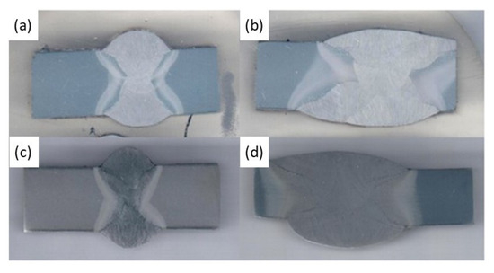
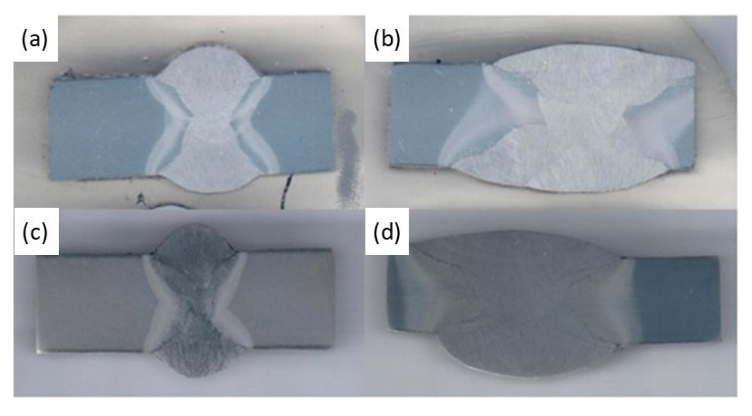
The weld contours of G1, S1, G2 and S2 are presented in Figure 3a–d. The SAW welded joints (S1 and S2) exhibit a larger weld width than GMAW (G1 and G2). The larger current value and heat input in SAW produce a relatively large melt pool, as demonstrated by the difference in weld width.

Figure 3. Low-magnification microstructure of welded joints (a) G1; (b) S1; (c) G2; (d) S2.

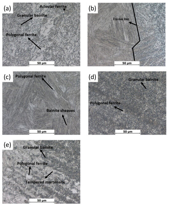
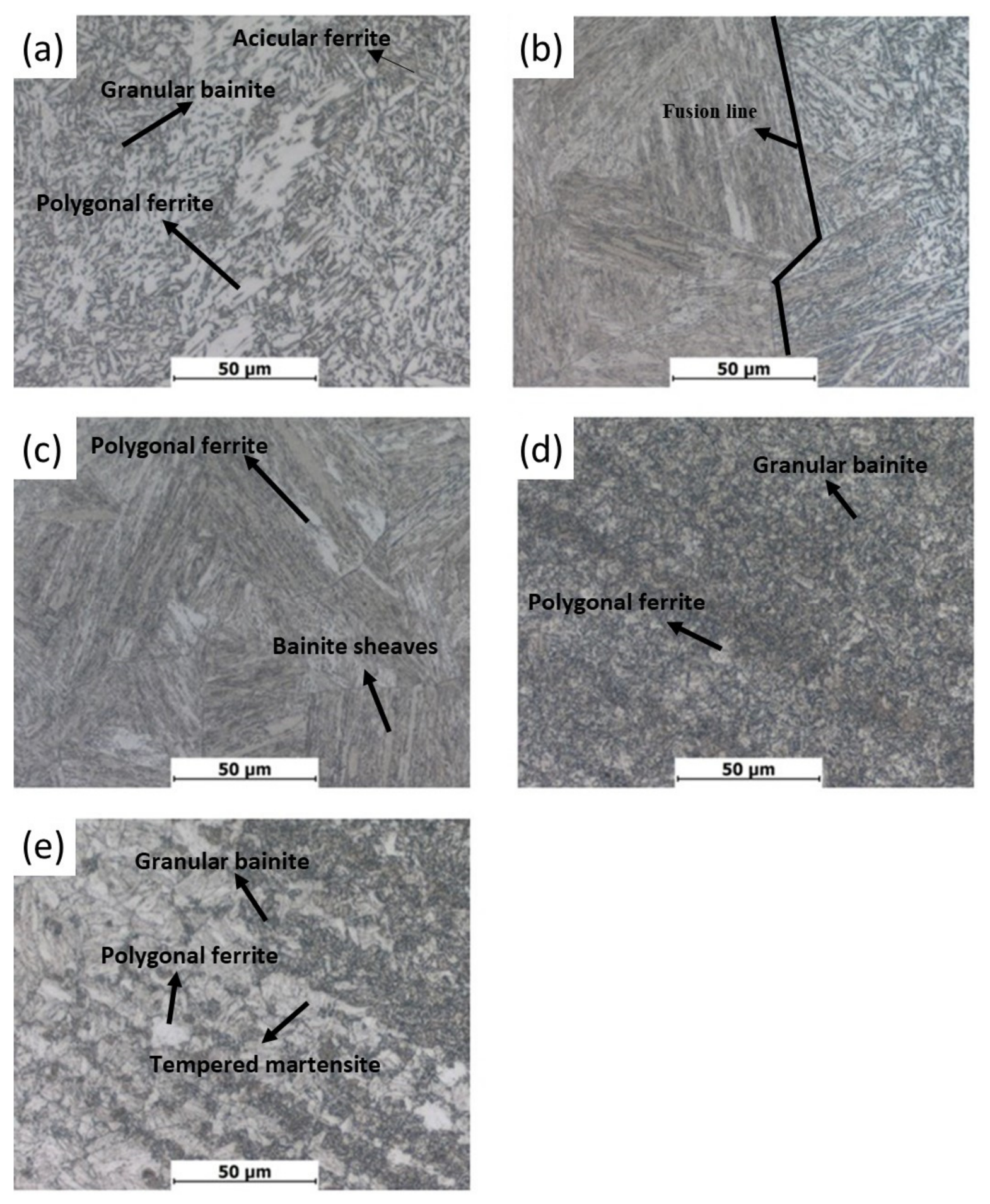
Figure 4 presents OM images of different regions of welded joints of the G1 specimen. The OM images of G2, S1 and S2 are in Figures S1–S3 in the Supplementary Information. Overall, all welded joints exhibit a distinct microstructural gradient from the weld to the base material. Despite the differences in processing conditions, the microstructural gradient remains consistent across all four conditions. For instance, in Figure 4a, the fusion zone primarily consists of acicular ferrite, granular bainite, and polygonal ferrite [25], which are typical characteristics of as-cast HSLA steel [26]. The fusion line clearly distinguishes the fusion zone (right side) and heat-affected zone (HAZ) (left side) by microstructure, as shown in Figure 4b. The fusion zone resembles as-cast weld metal, as discussed in Figure 4a, and the HAZ is characterized by coarse bainitic laths, consistent with the literature [27]. The coarse grain heat-affected zone (CGHAZ) and fine grain heat-affected zone (FGHAZ) (see Figure 4c,d exhibits microstructure resemble coarse bainitic laths arranged in sheaves and granular bainite, respectively. In addition, the FGHAZ also contains dispersed polygonal ferrite. The difference in peak temperature between CGHAZ and FGHAZ results in two distinct microstructures. CGHAZ has experienced a higher peak temperature than Ac_3r resulting in complete austenite transformation, followed by the formation of coarse bainitic laths upon cooling. Whereas, the FGHAZ experiences peak temperatures well below those of CGHAZ, leading to the formation of a fine bainitic microstructure and retained polygonal ferrite. Figure 4e shows the morphology of the intercritical heat-affected zone (ICHAZ). The heterogenous microstructure suggests partial austenite phase transformation during the welding process. As a result, the microstructure consists of untransformed polygonal ferrite embedded in granular bainite and tempered martensite constituents during cooling [28]. The microstructural evolution of weldments is consistent in G2, S1 and S2 (see Figures S1–S3) with minor variation in grain size caused from difference in processing conditions.

Figure 4. Optical microscopy (OM) images of G1 welded joints. (a) Weld seam; (b) fusion line; (c) coarse grain heat-affected zone (CGHAZ); (d) fine grain heat-affected zone (FGHAZ); (e) inter-critical heat-affected zone (ICHAZ).

3.2. Mechanical Behavior

3.2.1. Vickers Microhardness

Table 4 summarizes the average Vickers microhardness of all four specimens G1, G2, S1, and S2 measured across the four distinct weld zones, i.e., fusion zone, CGHAZ, FGHAZ and base alloy. The fusion zone and base alloy exhibit comparable hardness of 241–256 HV0.5 and 225–252 HV0.5, respectively. The hardness has increased in FGHAZ, reaching up to ~274 HV in G1. Further, CGHAZ exhibited the highest hardness among the weld zones, with the most pronounced hardening effect observed in G1 (339 HV) and S1 (306 HV). In contrast, G2 exhibited comparable average hardness in the fusion zone (256 HV), CGHAZ (257 HV), and FGHAZ (260 HV). These results indicate that distinct microstructural regions do not necessarily produce a monotonic hardness gradient, because it reflects the combined effects of phase constitution, microstructural scale, and local welding thermal history [29]. Therefore, the hardness may be varying from tempered base metal, depending on the relative phase fractions, substructure, and local welding thermal history.

Table 4. Average Vickers microhardness (HV) across weld zones of four welded joints.

Zone/Specimen	G1	S1	G2	S2
Fusion zone	250 ± 6	252 ± 6	256 ± 6	241 ± 8
Coarse grain heat-affected zone (CGHAZ)	339 ± 41	306 ± 15	257 ± 19	284 ± 14
Fine grain heat-affected zone (FGHAZ)	274 ± 7	271 ± 16	260 ± 14	251 ± 21
Base alloy	252 ± 8	235 ± 7	225 ± 15	250 ± 9

3.2.2. Tensile Properties

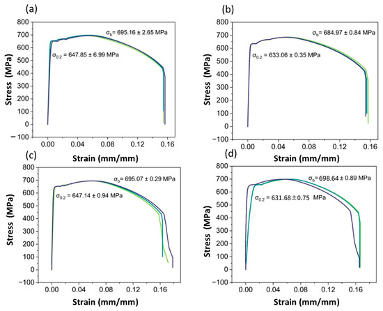
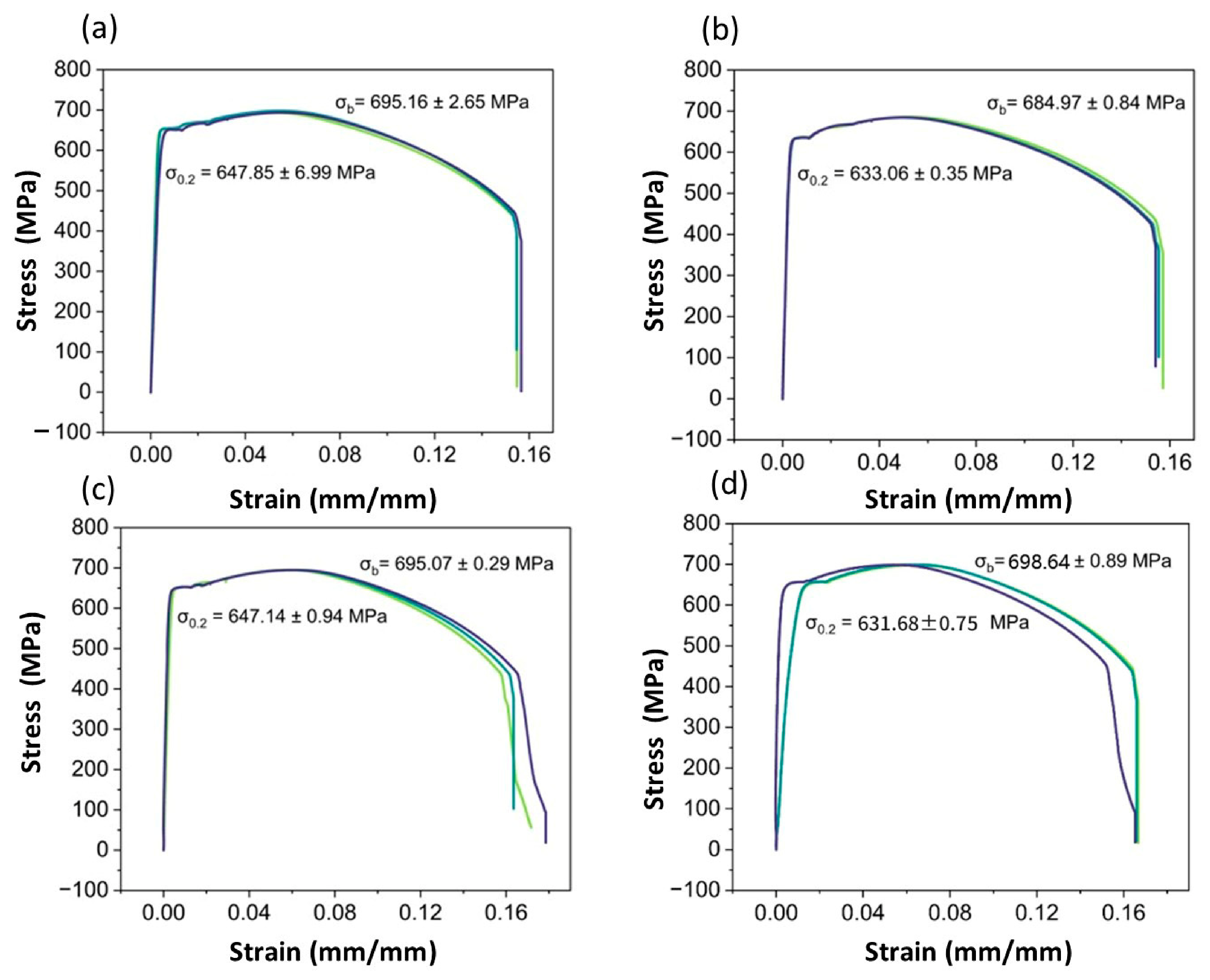
Figure 5a–d shows the engineering stress–strain curves of 10CrNi3MoV steel welded joints under four welding conditions. Specimens G1, G2, S1 and S2 exhibit comparable tensile response, with yield strengths of 631.68–647.85 MPa, ultimate tensile strengths (UTS) of 684.97–698.64 MPa, and tensile strains of 15.38–16.76%. These results indicate that the four welded-joint conditions maintained similar global tensile properties within the tested parameter range. However, because the welding process, heat input, and interpass temperature varied simultaneously among the four conditions, the present data do not isolate the independent effect of welding method on joint tensile performance. All tensile specimens fractured in the base metal rather than in the weld metal or HAZ. Table 5 exhibits the room-temperature tensile properties of the four welded joints.

Figure 5. Engineering stress–strain curves of welded joints: (a) G1; (b) S1; (c) G2; (d) S2. Dark green, light green and purple indicates parallel specimen test results of each welded joint.

Table 5. Tensile properties of 10CrNi3MoV welded joints.

Condition	Yield Strength (MPa)	Ultimate Tensile Strength (MPa)	Elongation (%)
G1	647.85 ± 6.99	695.16 ± 2.65	15.38 ± 0.10
G2	647.14 ± 0.94	695.16 ± 0.29	16.76 ± 0.88
S1	633.06 ± 0.35	684.97 ± 0.84	15.43 ± 0.15
S2	631.68 ± 0.75	698.64 ± 0.89	16.35 ± 0.02

3.3. High-Cycle Fatigue S–N Behavior

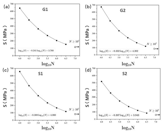
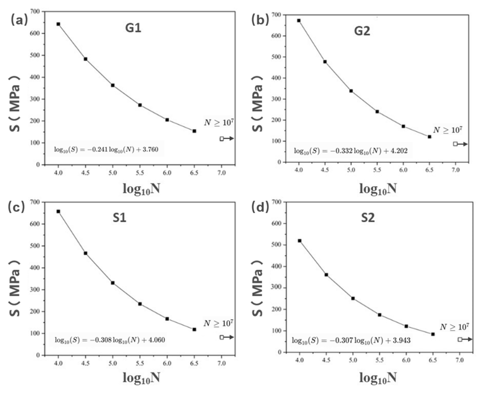
Figure 6 represents the S-N plot at the mean value of life cycles from data given in Table 6. The best-fitted curve was plotted using the Basquin relationship given in Equation (1).

$$\mathrm{l}\mathrm{o}\mathrm{g}S=A+b \mathrm{l}\mathrm{o}\mathrm{g}\left(N\right)$$

(1)

where $S \mathrm{i}\mathrm{s} \mathrm{n}\mathrm{o}\mathrm{m}\mathrm{i}\mathrm{n}\mathrm{a}\mathrm{l} \mathrm{s}\mathrm{t}\mathrm{r}\mathrm{e}\mathrm{s}\mathrm{s} \mathrm{a}\mathrm{n}\mathrm{d} N \mathrm{i}\mathrm{s} \mathrm{l}\mathrm{i}\mathrm{f}\mathrm{e} \mathrm{c}\mathrm{y}\mathrm{c}\mathrm{l}\mathrm{e}$.

Figure 6. S-N engineering curves of (a) G1, (b) G2, (c) S1, and (d) S2. Solid symbols represent fatigue failure data and were used for the Basquin regression. Open symbols with right-pointing arrows indicate run-out specimens that survived ${10}^7$ cycles without failure $\left(N\ge {10}^7\right)$; these run-out observations were excluded from the regression.

Table 6. Data representing mean experimental fatigue life at each stress level (n = 4–6) at stress ratio (R) of 0.1. N = number of fatigue cycles; σ_max = peak stress; σ_A = stress amplitude; σ_M = mean stress. * Indicates run-out specimens at fatigue life ≥ 10⁷ cycles and do not represent average mean life.

Specimen	Log10 (N)	σmax (MPa)	σmin (MPa)	σA (MPa)	σm (MPa)	Result (Fail/Runout)	n	Standard Deviation [log10N]
G1-1	4.42	490	49	220.5	269.5	Fail	5	0.17
G1-2	5.02	360	36	162	198	Fail	4	0.24
G1-3	5.62	270	27	121.5	148.5	Fail	6	0.10
G1-4	5.74	225	22.5	101.25	123.75	Fail	5	0.16
G1-5 *	≥7.00	116	11.6	52.12	63.73	Runout	4	—
S1-1	4.72	400	40	180	220	Fail	6	0.16
S1-2	5.2	300	30	135	165	Fail	5	0.12
S1-3	5.42	240	24	108	132	Fail	6	0.17
S1-4 *	≥7.00	84	8.4	37.8	46.2	Runout	4	—
G2-1	4.82	400	40	180	220	Fail	6	0.12
G2-2	4.98	350	35	157.5	192.5	Fail	4	0.18
G2-3	5.22	300	30	135	165	Fail	5	0.14
G2-4	5.42	250	25	112.5	137.5	Fail	5	0.13
G2-5 *	≥7.00	86	8.6	38.7	47.3	Runout	4	—
S2-1	4.86	300	30	135	165	Fail	5	0.18
S2-2	5.2	200	20	90	110	Fail	4	0.25
S2-3	5.8	150	15	67.5	82.5	Fail	4	0.22
S2-4 *	≥7.00	59	5.9	26.4	32.2	Runout	4	—

The welded joints have shown different fatigue resistance when processed under four different conditions. However, specimen G1 has shown better fatigue resistance than G2 and S1, while S2 exhibits the lowest resistance in the high-cycle region. G2 and S1 show similar behavior. Overall, the fatigue life cycle has shown a constant decrease with the increase in nominal stress, and no distinct endurance limit was established within the investigated fatigue-life range and the adopted 10⁷ -cycle run-out criterion. The nominal stress decreases with the increase in fatigue loading cycles, demonstrating an inverse fatigue strength and fatigue life relationship. The slope parameter $b$ in the Basquin equation provides an indication of the fatigue sensitivity to stress amplitude, with more negative values corresponding to a steeper decrease in allowable stress amplitude with increasing fatigue life. So G1 exhibited a notably less negative slope (b = −0.241) compared to G2 (−0.332), S1 (−0.308), and S2 (−0.307), indicating superior fatigue resistance at longer lives.

Table 7 shows calculated coefficients of determination (R²) for S-N fitting parameters. The S–N curve exhibited an excellent fit, with R² values ranging from 0.929 (S1 and S2) to 0.983 (G2). G2, with the highest R² of 0.983, showed the most consistent fatigue behavior among the four configurations.

Table 7. S–N fitting parameters and adjusted coefficient of determination (R²) for the four welded joint groups.

Condition	R2
G1	0.980
S1	0.995
G2	0.981
S2	0.936

3.4. Three-Dimensional Internal Defect Characterization

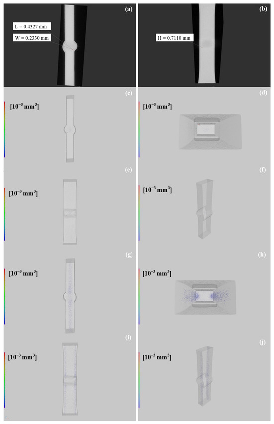
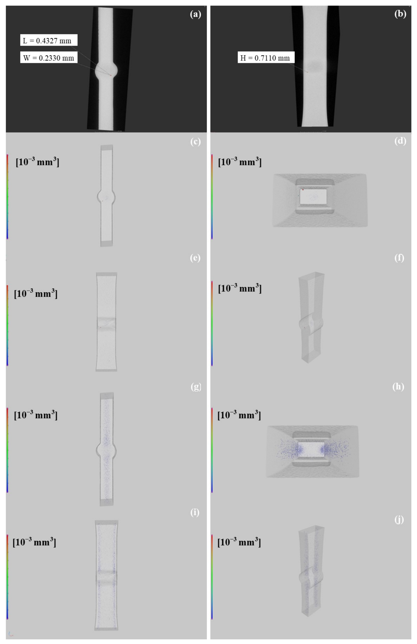
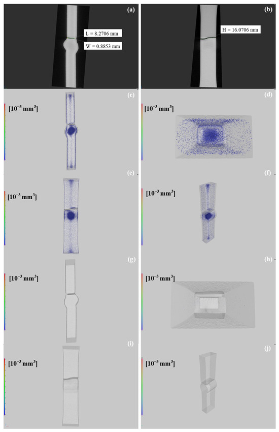
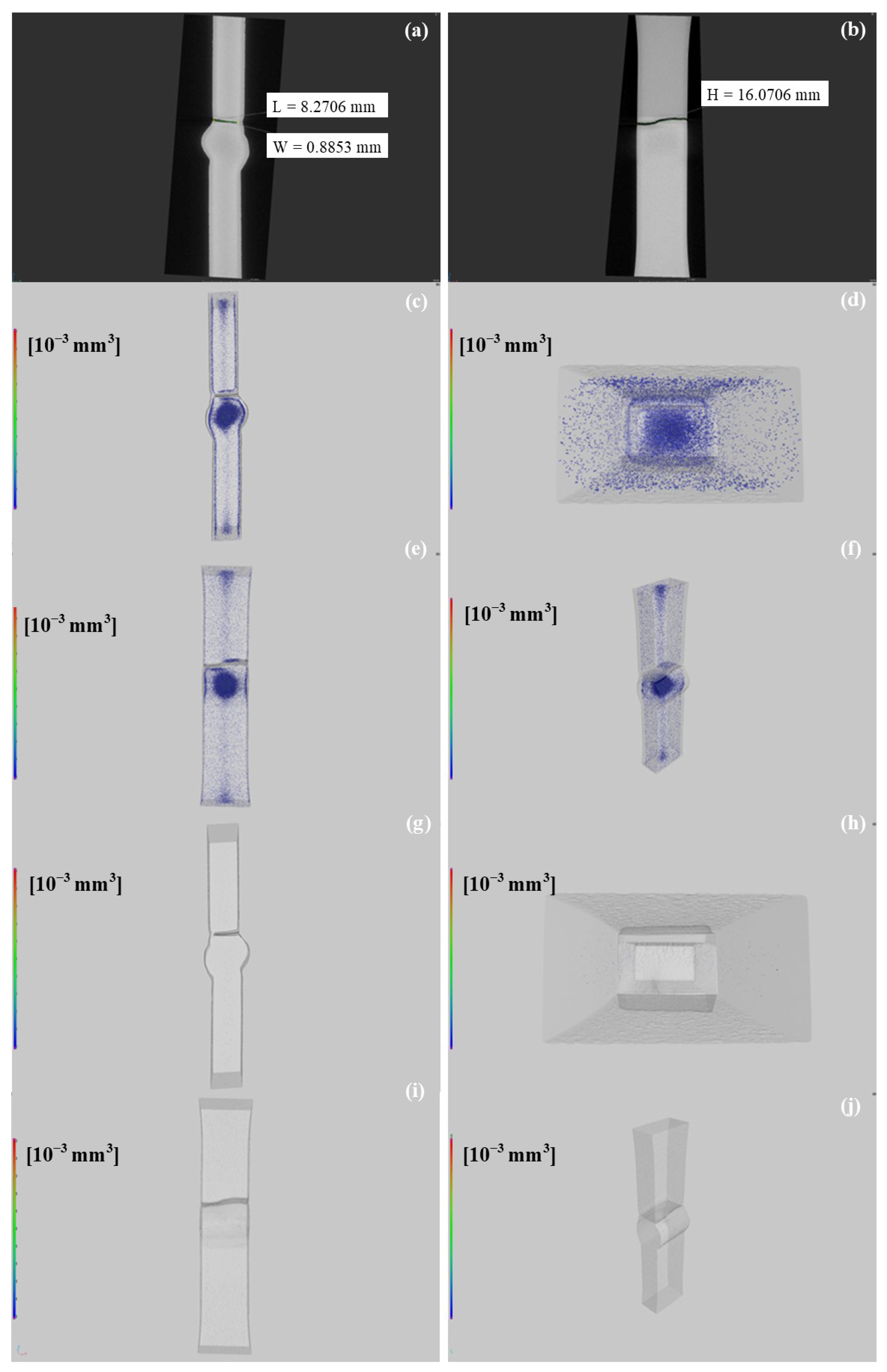
XCT analysis was performed on eight fatigue-tested specimens to characterize the three-dimensional internal defect populations, as summarized in Table 8. The XCT images are shown in Figure 7 and Figure 8, and S1–S9. The detected defects consisted predominantly of pores with spherical or irregular morphologies together with irregularly shaped inclusions concentrated near the fusion boundary. The internal pores are distributed and relatively small in size. No obvious large-size pore clusters or defects were identified. The XCT-resolved porosity volume fraction varied from 0.00044% to 0.18907% across the specimens, whereas inclusion volume fraction showed less variation. The results indicate that specimens G2-34 and S2-17 with pore volume fractions of 0.18907% and 0.07813% exhibit shorter cycle lives. Specimens S1-4 and S2-17 exhibited distinct fatigue lives of 211,000 and 29,200 cycles, under a peak stress of 300 MPa. This difference coincided with their different XCT-resolved porosity volume fractions, rather than by itself establishing a direct causal relation.

Table 8. X-ray computed tomography (XCT)-derived defect characteristics and fatigue lives of the investigated specimens.

Specimen	σmax (MPa)	Fatigue Life (Cycles)	Inclusion Volume Fraction (%)	Porosity Volume Fraction (%)	Outcome
G2-11	350	54,900	0.00122	0.00470	Failure
G2-13	300	260,300	0.00065	0.00667	Failure
G2-14	300	111,900	0.00264	0.02356	Failure
G2-28	400	51,909	0.00312	0.05226	Failure
G2-33	168	10,000,000	0.00942	0.00044	Run-out
G2-34	168	773,100	0.00062	0.18907	Failure
S2-17	300	29,200	0.01443	0.07813	Failure
S1-4	300	21,1000	0.01731	0.00254	Failure

Figure 7. G2-33 XCT images characterizing defects. Crack: (a) front and (b) side view. Porosity: (c) left view, (d) top view, (e) front view, (f) perspective. Inclusion: (g) left, (h) top, (i) front, and (j) perspective. Color indicates the intensity per unit volume and the progressive transition from blue (bottom) to red (top) color indicates the increase in defect volume.

Figure 8. G2-34 XCT images characterizing defects. Crack: (a) front and (b) side view. Porosity: (c) left view, (d) top view, (e) front view, (f) perspective. Inclusion: (g) left, (h) top, (i) front, and (j) perspective. Color indicates the intensity per unit volume and the progressive transition from blue (bottom) to red (top) color indicates the increase in defect volume.

To examine the association between defect population and fatigue life, paired-case comparisons were conducted under identical nominal stress. Accordingly, specimens from G2 (G2-33 and G2-34) were exposed to identical loading parameters (σ_max = 168 MPa, R = 0.1, f = 120 Hz). Specimen G2-33 survived the 10⁷-cycle run-out criterion, whereas specimen G2-34 failed after 773,100 cycles. Their porosity volume fractions were 0.00044% and 0.18907%, respectively, corresponding to an approximately 430-fold difference. Similarly, for G2-13 and G2-14 tested at ${\sigma }_{\mathrm{m}\mathrm{a}\mathrm{x}}=300 \mathrm{MPa}$, G2-14 exhibited a porosity volume fraction approximately 3.53 times that of G2-13 (0.02356% vs. 0.00667%) and a shorter fatigue life (111,900 vs. 260,300 cycles). These paired observations suggest that a greater internal pore population is associated with reduced fatigue life under identical loading conditions [30]. A greater pore population may increase the likelihood of a critically sized or critically located defect and can reduce the effective load-bearing area, thereby increasing local stress concentration. Nevertheless, the paired comparisons do not by themselves identify the specific defect that initiated cracking.

Pores can act as fatigue-crack initiation sites by producing local stress concentrations [31,32]. From a fracture mechanics perspective, the stress intensity factor ΔK at a near-surface is proportional to the square root of the defect size [33], as given below in Equation (2).

$$∆K=Y∆\sigma \sqrt{\pi a}$$

(2)

where $∆K$ stress intensity range, dimensionless constant, $∆\sigma$ difference in maximum and minimum load, and a is the defect radius.

To further evaluate mechanically relevant defect size, the largest pore diameter, projected defect size, and distance from the crack origin were determined for G2-13, G2-14, G2-33, and G2-34 (Table 9). Because fatigue loading was applied along the $z$-axis, the defect area was projected onto the plane perpendicular to the loading direction (the XY plane) and approximated as an ellipse for calculation of $\sqrt{area}$, as given in Equation (3) [34]:

$$A_{xy}={\displaystyle \frac{\pi d_x{d}_y}{4}},\sqrt{\mathrm{a}\mathrm{r}\mathrm{e}\mathrm{a}}=\sqrt{A_{xy}}.$$

(3)

Table 9. Specimens’ largest pore diameter, $\sqrt{\mathrm{a}\mathrm{r}\mathrm{e}\mathrm{a}}$ and distance from the nearest crack.

Specimen	Largest Pore Diameter (mm)	Estimated $\sqrt{\mathbf{a}\mathbf{r}\mathbf{e}\mathbf{a}}$	Spatial Relation of Largest Pore
G2-13	0.924	0.509	11.10 mm from crack origin
G2-14	0.628	0.447	9.24 mm from crack origin
G2-33	0.727	0.540	8.00 mm from nearest free surface
G2-34	1.400	0.630	12.48 mm from crack origin

The maximum estimated $\sqrt{area}$ values were approximately 0.540 and 0.630 mm for G2-33 and G2-34, indicating specimen with the shorter fatigue life contained both a much greater pore population and a larger projected defect. On the contrary, G2-13/G2-14 paired-case analysis suggests that the maximum projected defects of sizes 0.509 mm and 0.447 mm, respectively, do not vary monotonically with fatigue life. The corresponding defect dimensions were extracted directly from the XCT defect datasets.

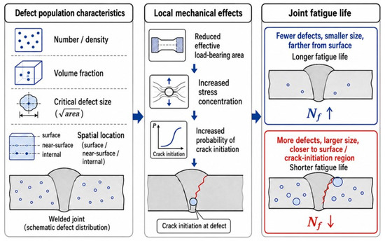
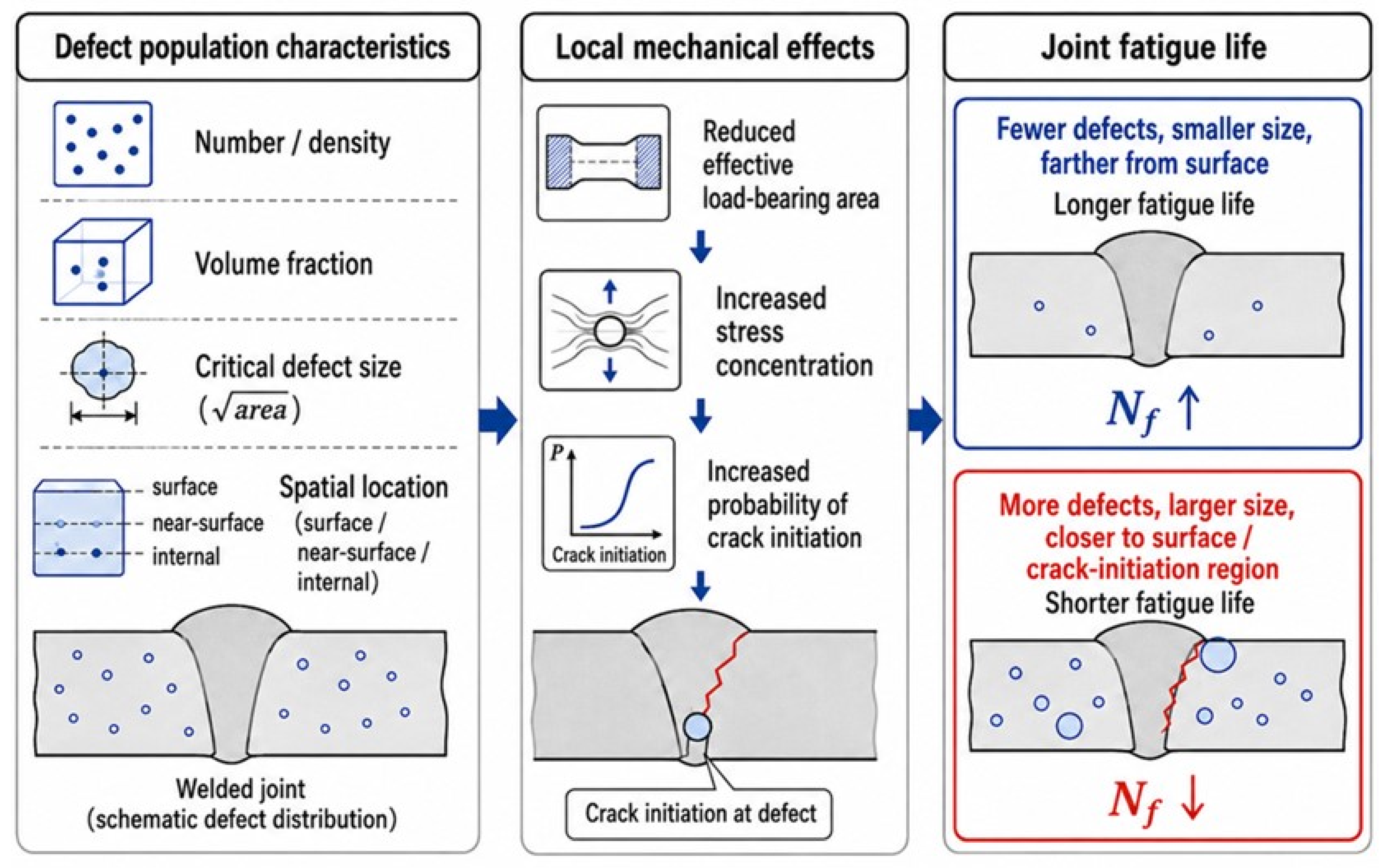
These results indicate that neither porosity volume fraction nor the largest defect size alone is sufficient to determine HCF life. Instead, the present paired comparisons should therefore be regarded as evidence of an association between XCT-resolved defects and fatigue response. Characterization of defect chemistry and morphology at the crack-initiation scale, together with XCT-based defect statistical analysis, may provide a robust method to develop defect-tolerant fatigue life predictive models. The schematic diagram highlights the defect characteristics; their influence on mechanical integrity and, consequently, fatigue life is given in Figure 9.

Figure 9. Schematic diagram explaining defect population characteristics, their mechanical effects and influence on fatigue life of welded joints. (download arrows in local mechanical effects indicate the process flow; whares upward and downward arrows in Joint fatigue life indicate increase and decrease in N_f).

3.5. Deformation Behavior

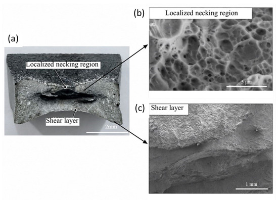
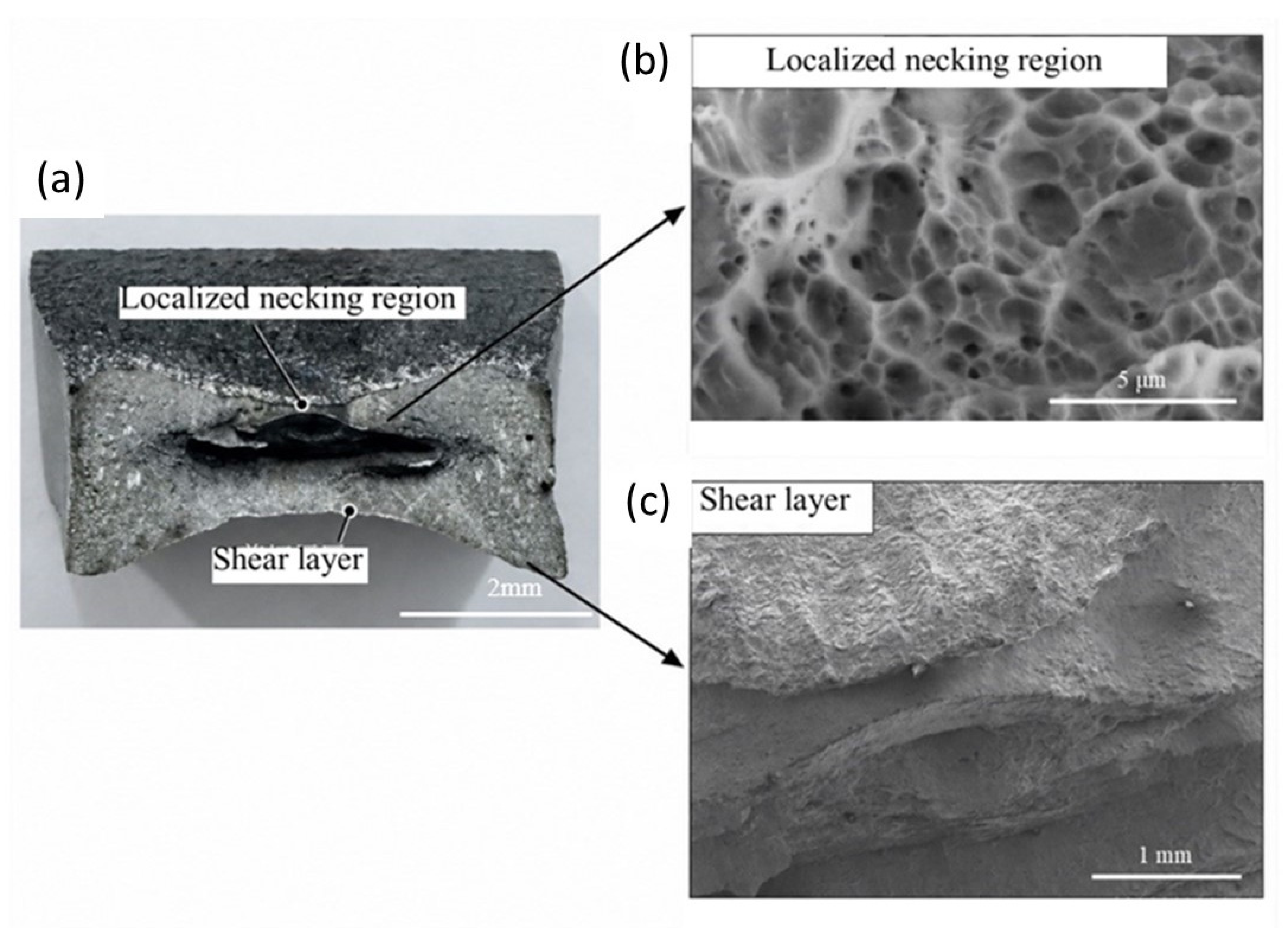
To reveal the fracture mechanism of welded joints, both tensile and fatigue fractures were characterized using SEM. Figure 10 shows the macroscopic surface morphology of the specimen after a tensile fracture, which clearly resembles the characteristics of local necking and shear lip. In Figure 10b, the magnified image shows numerous interconnected pits and micropores of varying sizes in a necked region. These features indicate that fracture primarily proceeds through the nucleation, growth, and coalescence of micropores. Further, the tear edges are observed in the shear lip region with significant plastic flow along the shear direction [35]. Overall, the specimen exhibits characteristics of both local necking and shear lip, demonstrating tensile and strong directional shear deformation, respectively.

Figure 10. SEM acquired tensile fracture images of the weld joint. (a) Macroscopic image; (b) localized necking region; (c) shear lip area.

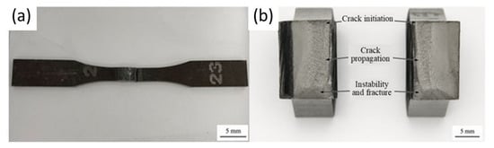
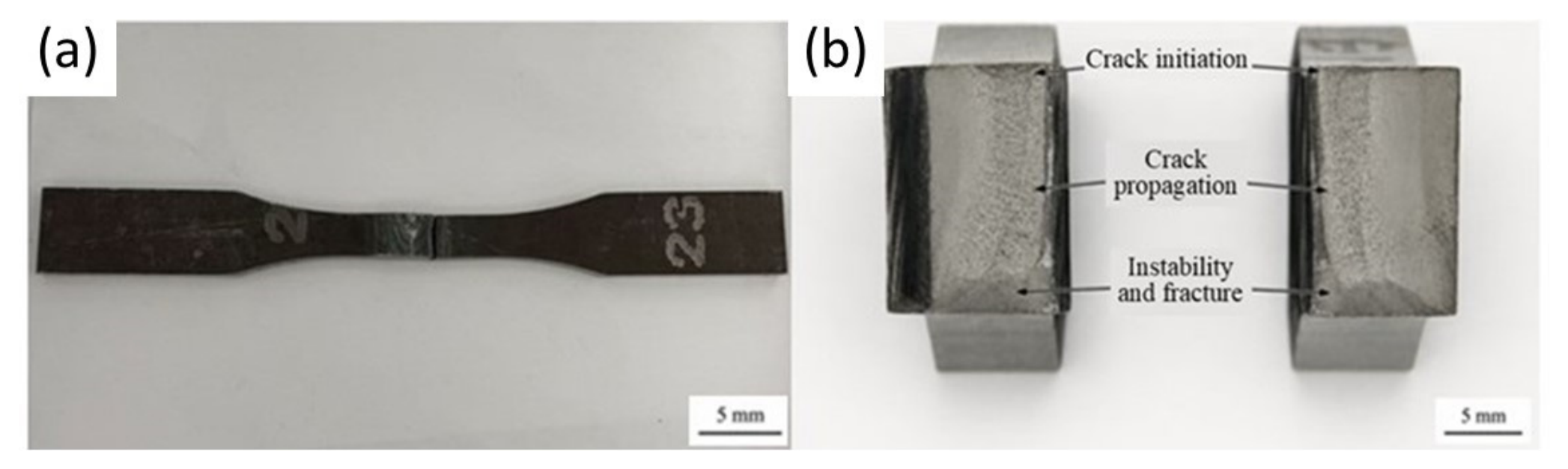
Unlike tensile fracture, fatigue-loaded fracture has failure points closer to the weld seam, as shown in Figure 11a. No obvious necking or plastic deformation appeared on the surface of the fracture specimen, which is consistent with the macroscopic characteristics of fatigue fracture [36]. From Figure 11b, the fracture can be divided into a fatigue crack source, crack propagation, and final fracture surface. Cracks first appear at geometrically stress-concentrated surfaces or subsurface, then gradually propagate into the cross-section under cyclic loading; When the remaining effective bearing area decreases to a critical level, the sample undergoes rapid instability leading to fracture [37]. Figure 11 macroscopically corresponds to the evolution of fatigue cracks from initiation to progressive propagation and final overload fracture.

Figure 11. Macroscopic morphology of fatigue specimen fracture and division of fracture zones: (a) overall morphology of fracture specimens; (b) macroscopic zoning of fatigue fractures.

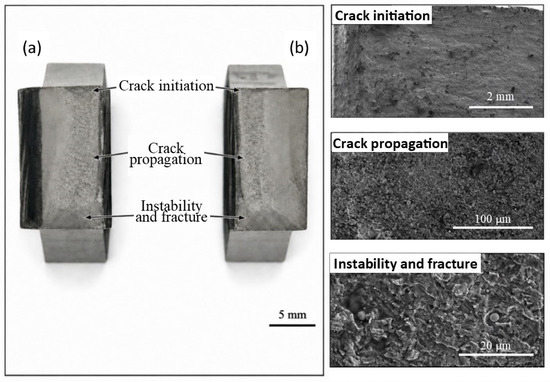
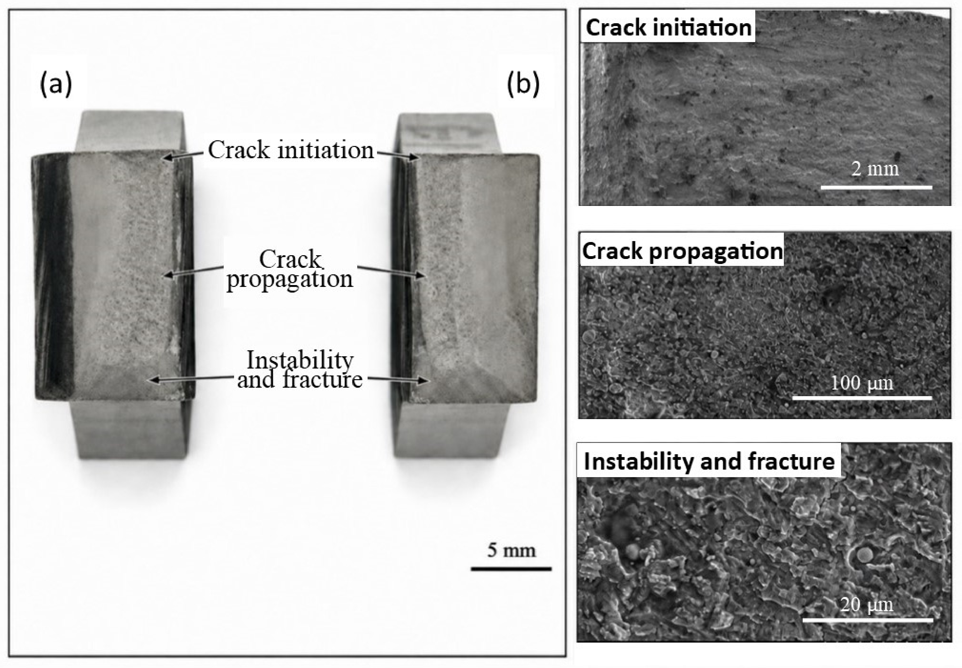
Figure 12 shows the magnified images indicating different fracture surfaces, as discussed. Figure 12a is an enlarged image of Figure 11b to reveal further details in macroscopic fracture features. The fracture surface appears relatively flat, with fine steps and undulating features along the crack propagation direction, suggesting fatigue cracks may have initiated at locally stress-concentrated sites on the surface and subsequently propagated inward into the cross-section [38]. The fracture surface contains fine steps, together with undulating traces in the crack-propagation direction. Such progression features are consistent with crack propagation during fatigue loading. No significant plastic deformation was observed, indicating stable crack propagation for a prolonged period. Additionally, the final fracture zone, located at the end of crack propagation, has significantly higher surface roughness, indicating severe plastic deformation due to structural instability. As the crack reaches a certain size, the effective load- bearing area becomes sufficiently small to bear external loads, causing a certain degree of local plastic deformation.

Figure 12. Macroscopic morphology of fatigue fracture at welded joints and SEM morphology in different regions. (a) macro surface image; (b) SEM magnified images characterizing different fracture regions.

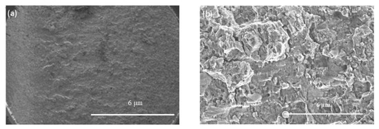
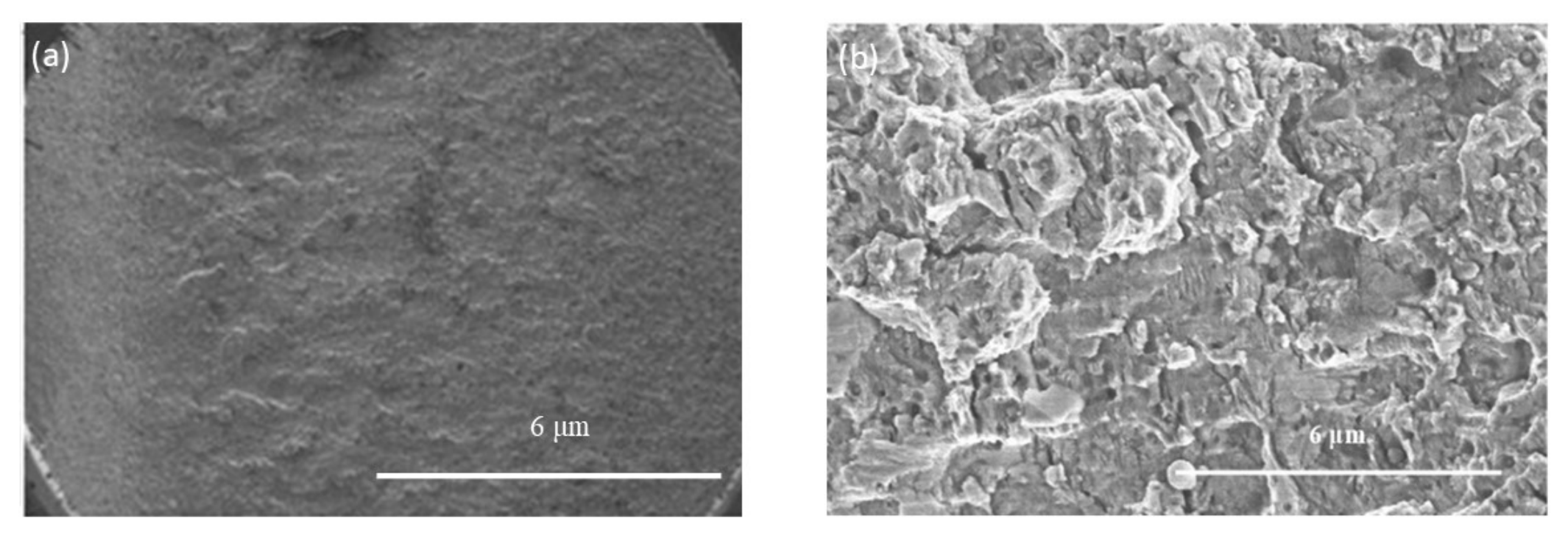
Figure 13 shows the SEM images of the fatigue fracture specimen. The fracture occurred in the weld-centered region, close to the fusion zone/fusion boundary. The smoother surface corresponds to stable fatigue-crack propagation, whereas the rougher morphology with tearing ridges and irregular facets represents the later-stage or final overload fracture.

Figure 13. SEM morphology in typical fatigue fracture regions. (a) fatigue crack propagation region; (b) crack propagation instability leading to complete fracture.

Comparison of the fractographic observations with the XCT defect locations showed that the largest XCT-detected pore did not coincide with the crack origin in the examined failed specimens. The largest pores in G2-13, G2-14, and G2-34 were located 11.10, 9.24, and 12.48 mm from the crack origin, respectively (Table 9). Thus, the present data do not demonstrate that the largest detected pore was the crack-initiating defect. Fatigue initiation may instead be governed by a smaller but more critically located defect, a surface or subsurface stress concentrator, or a feature below the XCT detection/segmentation capability. Accordingly, the porosity–fatigue relationship is interpreted here at the defect-population level rather than as a direct one-to-one correspondence between the largest XCT-detected defect and the fracture origin.

4. Conclusions

(1) The multi-pass 10CrNi3MoV high-strength low-alloy (HSLA) steel welded joints, fabricated by gas metal arc welding (GMAW; G1 and G2) and submerged arc welding (SAW; S1 and S2), exhibited characteristic fusion zone (FZ), coarse-grained heat-affected zone (CGHAZ), fine-grained heat-affected zone (FGHAZ), and base metal (BM). Among these regions, the CGHAZ exhibited the highest microhardness, reaching 339 HV in G1, which was associated with variations in the welding thermal cycle, cooling rate and resulting phase constituents. The other regions showed relative hardness values ranging from 225 to 274 HV. The overall microstructure characteristics were comparable among G1, G2, S1, and S2.

(2) The tensile properties were comparable among all investigated welded joints, with yield strengths of 631.68–647.85 MPa, ultimate tensile strengths of 684.97–698.64 MPa, and elongations of 15.38–16.76%. All tensile specimens fractured in the base metal rather than in the weld metal or heat-affected zone. Because the welding process, heat input, and interpass temperature varied simultaneously, the independent effect of welding method cannot be isolated from the present dataset.

(3) The high cycle fatigue (HCF) behavior was evaluated at a stress ratio (R) of 0.1 and a frequency of 120 Hz. The experimental S–N data were successfully described using the Basquin relationship. The fitted curves demonstrate that G1 exhibited the highest fatigue strength over the investigated fatigue-life range, followed by G2 and S1, while S2 exhibited the lowest fatigue strength. At 10⁶ cycles, the estimated fatigue strengths from the fitted Basquin relationships were approximately 205, 169, 166, and 120 MPa for G1, G2, S1, and S2, respectively.

(4) X-ray computed tomography (XCT) revealed an association between the internal defect population and HCF life. In a paired-case comparison, an approximately 428-fold increase in porosity volume fraction was accompanied by a reduction in fatigue life from run-out condition (>10⁷) to 773,100 cycles at a maximum stress (σ_max) of 168 MPa. This observation indicates that differences in volumetric internal defects may substantially influence HCF performance, even when the welded joints exhibit comparable tensile properties.

(5) Among the investigated welding conditions, G1 exhibited the highest HCF strength. The corresponding processing conditions consisted of a current of 210–230 A, voltage of 24–28 V, welding speed of 25–35 cm·min⁻¹, linear energy of approximately 11.4 kJ·cm⁻¹, and an inter-pass temperature of 120–140 °C. This G1 condition may therefore serve as a baseline welding procedure for fatigue-critical 10CrNi3MoV components within the scope of investigated parameters in this study. The results also suggest that the conditions associated with higher linear energy, particularly S2 (34.6 kJ·cm⁻¹), exhibited lower HCF strength; however, the individual effects of linear energy, welding method, and inter-pass temperature cannot be separated from the present experimental design. Accordingly, optimization of fatigue performance should emphasize control of welding conditions and minimization of internal volumetric defects.

(6) The combined XCT characterization and HCF testing provide experimental evidence to support the development of a quantitative relationship between three-dimensional weld-defect characteristics and fatigue life in 10CrNi3MoV welded joints. Future studies should systematically investigate the effects of weld methods and parameters on defect population characteristics to provide the basis for introducing machine-learning-assisted models for welding-parameter optimization and HCF-life prediction.

References

- Song, W.; Liu, X.; Xu, J.; Fan, Y.; Shi, D.; He, M.; Wang, X.; Berto, F. Fatigue fracture assessment of 10CrNi3MoV welded load-carrying cruciform joints considering mismatch effect. Fatigue Fract. Eng. Mater. Struct. 2021, 44, 1739–1759. [Google Scholar] [CrossRef] [Scilit]
- Corigliano, P.; Crupi, V. Review of Fatigue Assessment Approaches for Welded Marine Joints and Structures. Metals 2022, 12, 1010. [Google Scholar] [CrossRef] [Scilit]
- van Lieshout, P.S.; den Besten, J.H.; Kaminski, M.L. Multiaxial fatigue assessment of welded joints in marine structures:Literature overview of progress in academia and engineering practice. Int. Shipbuild. Prog. 2018, 65, 29–71. [Google Scholar] [CrossRef] [Scilit]
- Hobbacher, A. The new IIW recommendations for fatigue assessment of welded joints and components—A comprehensive code recently updated. Int. J. Fatigue 2009, 31, 50–58. [Google Scholar] [CrossRef] [Scilit]
- DNVGL-CG-0129; Fatigue Assessment of Ship Structures. DNV GL AS: Høvik, Norway, 2015.
- Hu, L.H.; Huang, J.; Li, Z.G.; Wu, Y.X. Effects of preheating temperature on cold cracks, microstructures and properties of high power laser hybrid welded 10Ni3CrMoV steel. Mater. Des. 2011, 32, 1931–1939. [Google Scholar] [CrossRef] [Scilit]
- Song, W.; Liu, X.; Berto, F.; Razavi, S.M.J. Low-Cycle Fatigue Behavior of 10CrNi3MoV High Strength Steel and Its Undermatched Welds. Materials 2018, 11, 661. [Google Scholar] [CrossRef] [Scilit]
- Song, W.; Liu, X.; Zhou, G.; Wei, S.; Shi, D.; He, M.; Berto, F. Notch energy-based low and high cycle fatigue assessment of load-carrying cruciform welded joints considering the strength mismatch. Int. J. Fatigue 2021, 151, 106410. [Google Scholar] [CrossRef] [Scilit]
- Song, W.; Wang, P.; Wan, D.; Qian, G.; Correia, J.; Berto, F. Fatigue crack growth behavior of Ni-Cr-Mo-V steel welded joints considering strength mismatch effect. Int. J. Fatigue 2021, 151, 106389. [Google Scholar] [CrossRef] [Scilit]
- Wei, S.; Jingjing, L.; Xuesong, L.; Ping, W.; Di, W.; Filippo, B. Fatigue crack growth rates of 10CrNi3MoV steel welded joints considering the stress ratio. In Proceedings of the IGF26—26th International Conference on Fracture and Structural Integrity, Turin, Italy, 26–28 May 2021; pp. 802–808. [Google Scholar]
- Song, W.; Huang, T.; Zhou, G.; Xie, H.; Wang, X.; He, M.; Shi, D. Fatigue cracking propagation behavior of 10CrNi3MoV steel mismatched welded joints at sub-temperature. Eng. Fract. Mech. 2025, 313, 110669. [Google Scholar] [CrossRef] [Scilit]
- Li, S.; Liu, Q.; Rui, S.-S.; Li, X.; Hu, M.; Li, K.; Sun, Q.; Cai, Z.; Pan, J. Fatigue crack initiation behaviors around defects induced by welding thermal cycle in superalloy IN617B. Int. J. Fatigue 2022, 158, 106745. [Google Scholar] [CrossRef] [Scilit]
- Kang, G.; Luo, H. Review on fatigue life prediction models of welded joint. Acta Mech. Sin. 2020, 36, 701–726. [Google Scholar] [CrossRef] [Scilit]
- Liu, F.; Chen, Y.; He, C.; Li, L.; Wang, C.; Wang, Q.; Liu, Y. Microstructure and pore sensitivities in very high cycle fatigue behaviors of titanium alloy welded joints under stress ratios. Eng. Fract. Mech. 2024, 295, 109801. [Google Scholar] [CrossRef] [Scilit]
- Liu, F.; Chen, Y.; Li, L.; Wang, C.; Wang, Q.; Liu, Y. Influence of welded pores on fatigue behavior of TC17 titanium alloy welded joints subjected to gigacycle regime at room and high temperatures. J. Mater. Sci. Technol. 2024, 178, 1–21. [Google Scholar] [CrossRef] [Scilit]
- Crupi, V.; Epasto, G.; Guglielmino, E.; Marinò, A. Influence of Weld-Porosity Defects on Fatigue Strength of AH36 Butt Joints Used in Ship Structures. Metals 2021, 11, 444. [Google Scholar] [CrossRef] [Scilit]
- Zhao, X.; Dongpo, W.; Deng, C.; Liu, Y.; Zongxian, S. The fatigue behaviors of butt welds ground flush in the super-long life regime. Int. J. Fatigue 2012, 36, 1–8. [Google Scholar] [CrossRef] [Scilit]
- GJB 1663A-2018; Specification for 10CrNi3MoV, 10CrNi3MoCu and 10CrNi2MoCu Steel Plates for Military Ship. Equipment Development Department of the Central Military Commission: Beijing, China, 2018.
- GB/T 39281-2020; Wire Electrodes, Wires, Rods and Deposits for Gas Shielded Arc Welding of High Strength Steels. Standardization Administration of China: Beijing, China, 2020.
- GB/T 36034-2018; Solid Wire Electrodes, Tubular Cored Electrodes and Electrode/Flux Combinations for Submerged Arc Welding of High Strength Steels. Standardization Administration of China: Beijing, China, 2018.
- GB/T 4340.1-2024; Metallic Materials—Vickers Hardness Test—Part 1: Test Method. State Administration for Market Regulation: Beijing, China, 2024.
- GB/T 228.1-2021; Metallic Materials—Tensile Testing—Part 1: Method of Test at Room Temperature. State Administration for Market Regulation: Beijing, China, 2021.
- ISO 6892-1; Metallic Materials—Tensile Testing—Part 1: Method of Test at Room Temperature. International Organization for Standardization: Geneva, Switzerland, 2019.
- GB/T 3075-2021; Metallic Materials—Fatigue Testing—Axial Force-Controlled Method. Standardization Administration of China: Beijing, China, 2021.
- Shao, Y.; Liu, C.; Yan, Z.; Li, H.; Liu, Y. Formation mechanism and control methods of acicular ferrite in HSLA steels: A review. J. Mater. Sci. Technol. 2018, 34, 737–744. [Google Scholar] [CrossRef] [Scilit]
- Oliveira, B.F.d.; Oliveira, M.P.; Terrones, L.A.H.; Azevedo, M.G.d.; Godefroid, L.B. Microstructure and mechanical properties of as-cast and annealed high strength low alloy steel. J. Mater. Sci. Res. 2019, 8, 1. [Google Scholar] [CrossRef] [Scilit]
- Zhang, S.; Wang, Y.; Zhu, M.; Zhang, Z.; Nie, P.; Li, Z. Relationships among Charpy impact toughness, microstructure and fracture behavior in 10CrNi3MoV steel weld joint. Mater. Lett. 2020, 281, 128328. [Google Scholar] [CrossRef] [Scilit]
- Olson, D.L.; Siewert, T.A.; Liu, S.; Edwards, G.R. (Eds.) Welding, Brazing, and Soldering; ASM International: Materials Park, OH, USA, 1993; Volume 6. [Google Scholar]
- Nadimi, N.; Pouranvari, M.; Ansari, R.; Pouranvari, M. Understanding fusion zone hardness in resistance spot welds for advanced high strength steels: Strengthening mechanisms and data-driven modeling. J. Mater. Res. Technol. 2023, 26, 5549–5565. [Google Scholar] [CrossRef] [Scilit]
- Ahlqvist, M.; Norman, V.; Leidermark, D. Effect of fatigue-initiating defect area measurement on defect size distributions and fatigue assessment of ductile cast iron. Int. J. Fatigue 2026, 207, 109499. [Google Scholar] [CrossRef] [Scilit]
- Schönbauer, B.M.; Ghosh, S.; Kömi, J.; Frondelius, T.; Mayer, H. Influence of small defects and nonmetallic inclusions on the high and very high cycle fatigue strength of an ultrahigh-strength steel. Fatigue Fract. Eng. Mater. Struct. 2021, 44, 2990–3007. [Google Scholar] [CrossRef] [Scilit]
- Cheng, Y.; Wang, T.; Xue, G.; Wang, R. The Statistical analysis on the Paris’s Fatigue Model Parameters and Prediction on Fatigue Crack Growth Life of 10Ni5CrMoV Steel and Its Joint. Dev. Appl. Mater. 2019, 34, 1–6. [Google Scholar] [CrossRef]
- Moore, P.; Booth, G. 12—Weld fatigue assessment. In The Welding Engineer’s Guide to Fracture and Fatigue; Woodhead Publishing: Oxford, UK, 2015; pp. 175–184. [Google Scholar]
- Otero, S.; Álvarez, G.; Sicre, J.; Soto, C.; Rodríguez, C. From √A to Elliptical Defects: Refining Murakami’s Model for Fatigue Prediction in Sintered Steels. Metals 2026, 16, 100. [Google Scholar] [CrossRef] [Scilit]
- Klenam, D.E.P.; Oghenevweta, J.E.; Soboyejo, W.O. Fatigue of Single/Multiple Semi-Elliptical Cracks. In Comprehensive Structural Integrity, 2nd ed.; Aliabadi, M.H.F., Soboyejo, W.O., Eds.; Elsevier: Oxford, UK, 2023; pp. 53–72. [Google Scholar]
- England, A.; Gorash, Y.; Toumpis, A. Assessing the Very High Cycle Fatigue Behavior and Frequency Effect of Structural Steel Welds. Fatigue Fract. Eng. Mater. Struct. 2025, 48, 1529–1541. [Google Scholar] [CrossRef] [Scilit]
- Becker, W.T.; Shipley, R.J. (Eds.) Fatigue Failures. In Failure Analysis and Prevention; ASM International: Materials Park, OH, USA, 2002; Volume 11. [Google Scholar]
- Lynch, S.P. Progression markings, striations, and crack-arrest markings on fracture surfaces. Mater. Sci. Eng. A 2007, 468–470, 74–80. [Google Scholar] [CrossRef] [Scilit]
Disclaimer/Publisher’s Note: The statements, opinions and data contained in all publications are solely those of the individual author(s) and contributor(s) and not of MDPI and/or the editor(s). MDPI and/or the editor(s) disclaim responsibility for any injury to people or property resulting from any ideas, methods, instructions or products referred to in the content. |
© 2026 by the authors. Licensee MDPI, Basel, Switzerland. This article is an open access article distributed under the terms and conditions of the Creative Commons Attribution (CC BY) license.