


Abstract
Wear occurs in sliding bearings as they often operate under mixed friction conditions in heavy-duty applications. Over the years, this has led to the development of wear simulations to predict wear evolution in sliding bearings. As part of wear evolution, bearing surface topography changes, and the bearing clearance varies due to temperature rise. For realistic wear predictions, both the surface topography changes and thermal effects must be considered. However, existing wear simulations do not accurately account for thermal effects during mixed friction. Effects such as local and transient temperature rise and thermal expansion alter bearing contact conditions (clearance) and thus influence wear evolution. Since these effects are not accurately modelled, realistic wear prediction in sliding bearings remains challenging with current approaches. Therefore, this paper introduces the extension of wear simulations by local and transient modelling of bearing temperature and clearance changes. The novelty lies in enabling the simultaneous consideration of transient thermal changes and surface topography changes during wear evolution. This enables a more realistic prediction of wear development in sliding bearings which can be applied to evaluate wear safety in bearing designs. The thermal wear simulation is validated using experimental measurement of friction torque, bearing temperature, and wear volume obtained from a radial sliding bearing test bench.
1. Introduction
Sliding bearings are widely used in heavy-duty applications because they provide a compact design and high load-carrying capacity. Typical examples of heavy-duty applications include engine bearings in heavy-duty trucks [1,2], planetary gear bearings in wind turbine gearboxes [3,4] and stern tube bearings in marine propulsion systems [3,5,6]. Such applications include operating scenarios with frequent start-stop events [7], and mechanical overloading [6]. Under such operating conditions the bearing may operate under high loads at low rotational speeds. Normally, sliding bearings operate under hydrodynamic lubrication, where the sliding surfaces are separated by a fluid film. However, high loads combined with low speeds hinder the formation of a stable fluid film and prevent complete separation of sliding surfaces. As a result, contact between roughness asperities on the sliding surfaces occurs, a lubrication regime known as mixed friction. Mixed friction leads to heat generation and material removal, also known as abrasive wear. Under severe mixed friction, excessive heat generation can also cause overheating and adhesive wear on the bearing. Both adhesive and abrasive wear are the most frequent damage mechanisms in sliding bearings and thus pose a major challenge for bearing operating life [8,9]. A fundamental understanding of wear evolution over time is required to determine the operating condition-dependent severity of wear. This understanding can further be used to evaluate the wear safety of sliding bearing designs. For this purpose, iterative wear simulations are developed to predict wear generation in sliding bearings.
Each iteration in a wear simulation consists of an elasto-hydrodynamic (EHD) simulation, a contact model to consider mixed friction and a wear model [10,11,12,13]. The EHD simulation and contact model are used to calculate local asperity pressure on the bearing running surface. Based on occurring asperity contact pressure, a local wear rate is determined using a wear model. After each iteration, the bearing contour is modified according to the calculated wear depth and updated in the EHD simulation for the next iteration. In this way, iterative wear simulations can model wear evolution over time [5,11]. Wear evolution in sliding bearings starts with an initial running-in phase [14], where the initial wear rate decreases non-linearly with time. Overtime, the bearing surface is smoothened due to wear, resulting in linear wear progression. To model run-in behaviour in sliding bearings, it is important to consider wear at both the macroscopic (contour) scale and microscopic (surface roughness) level [10,13,15,16]. König [12] developed a numerical method to model the reduction in surface roughness during wear processes and integrated this roughness variation into wear simulations. Therefore, the surface topography changes during run-in wear can be realistically modelled using wear simulations that incorporate a wear-and-roughness model [12,15,17,18]. The evolution of bearing contact conditions is a key aspect of the run-in process. In wear simulations, this evolution is represented by a decrease in bearing asperity contact pressure over time [12,17]. Among the available contact models for calculating asperity contact pressure (), the Greenwood–Tripp model [19] is the most commonly used in practical applications. This model combines surface parameters—such as the standard deviation of asperity heights, asperity summit radius and asperity peak density—into an elastic factor () to calculate [20]. Although no standardized method exists to determine the exact value of , studies have identified a range of values based on different surface parameters [21]. The relationship between the -factor and is directly proportional [19]. During run-in, surface roughness decreases over time, and the value of , which depends on surface parameters, must also change. However, in existing wear simulations, the -factor is typically kept constant [10,12,13,15,18]. For a realistic modelling of run-in behaviour in sliding bearings, the -factor should vary over time in proportion to the evolving surface roughness.
In addition to surface topography changes, thermal effects during run-in wear further influence the bearing contact conditions. Mixed friction is associated with increased friction and, consequently, increased heat generation within the bearing [22]. Heat generation increases the temperature in the sliding surfaces and the lubricant. As temperature rises, the lubricant viscosity decreases, which reduces its load-carrying capacity. The sliding surfaces also undergo thermal expansion. Together, reduced lubricant viscosity and thermal expansion significantly influence the bearing clearance and contact conditions [23,24]. Changes in clearance and contact conditions, in turn, affect the wear intensity and its evolution over time. For realistic prediction of wear in sliding bearings, transient evolution of bearing clearance and contact conditions is influential. Modelling this evolution requires incorporating transient changes in temperature and thermal expansion, and temperature-dependent lubricant viscosity into wear simulations. Previous studies have considered thermal effects in wear simulations to a certain extent. Ding [25] integrated thermo-elastohydrodynamic (TEHD) simulations into wear simulations to account for heat transfer between the contact partners and lubricant. However, the temperature distribution within the bearing and the surrounding structures cannot be accurately modelled using the heat transfer model in TEHD simulations [26]. In this heat transfer model, the bearing structure is represented by layered discs rather than the actual system geometry [23,26]. Therefore, TEHD simulations are suitable for modelling heat transfer between the bearing, lubricant and shaft, but are limited in predicting realistic structural temperature distributions. Moreover, the approach proposed by Ding considered only a steady state energy equation and neglected thermal expansion. Therefore, the transient evolution of bearing temperature and clearance cannot be accurately modelled. This in turn leads to inaccurate prediction of asperity contact pressure, and subsequently, the wear over time. Consequently, the wear simulation was not validated, as no comparisons with experimentally measured wear depth or wear volume were performed. Prölß [20,24] introduced transient temperature calculations into wear simulations using an analytical heat balance equation. The transient bearing temperature evolution was predicted with good accuracy. However, thermal expansion was also neglected by them. As a result, the wear simulation showed a large error in wear volume of 20–30% for most operating points [24]. Thermal expansion of the sliding surfaces alters the bearing contact zone and therefore strongly influences wear volume generation. The geometry, mechanical and thermal constraints of the bearing housing significantly affect temperature distribution, local bearing thermal expansion and resulting contact conditions. Similar to heat transfer models in TEHD simulations, analytical heat balance equations can only represent simplified structures and boundary conditions. Therefore, such equations are limited in modelling the temperature distributions in complex bearing structures [27]. Finite element (FE) models can instead be used to compute transient temperature distribution and local thermal expansion while accounting for realistic bearing surroundings [28]. In summary, existing sliding bearing wear simulations can accurately model surface topography changes, but do not adequately capture the influence of thermal effects on bearing contact conditions. In particular, local and transient changes in temperature and thermal expansion, while considering complex surrounding structure, are not modelled. Furthermore, the influence of surface roughness evolution on the -factor in contact modelling is not considered. The use of a constant -factor for asperity contact calculations in wear simulations limits the accurate representation of contact evolution over time. As a result, realistic prediction of wear volume evolution over time remains limited due to insufficient accuracy in thermal modelling and contact calculations.
To address this gap in the literature, this paper focuses on extending an existing isothermal wear simulation tool by incorporating transient and local calculations of temperature and thermal expansion of sliding surfaces. These thermal effects are modelled using FE simulations. In addition, TEHD modelling is applied instead of the previously used EHD model to account for local temperature-dependent changes in lubricant viscosity. In addition, the contact modelling is improved by allowing a time-dependent local variation in the elastic -factor to simulate run-in behaviour. The existing iterative wear simulation tool already accounts for surface topography changes at both macroscopic and microscopic levels [12,17,18]. The novelty of this work lies in coupling the wear simulation with transient thermal FE models, and improving contact modelling by local variations in the -factor. This enables a more accurate representation of the temporal evolution of bearing contact conditions and hence, improves the prediction of wear volume generation. The proposed approach also enables simulation of transient run-in characteristics through the temporal and local evolution of -factor in the contact model. The proposed thermal wear simulation is validated by comparison with experimental measurements of wear volume, bearing temperature, and friction torque obtained from a radial sliding bearing test bench. These experiments were previously conducted by Decker et al. [18]. A detailed description of the modelling extensions in the proposed approach and the validations results are presented in the following sections.
2. Materials and Methods
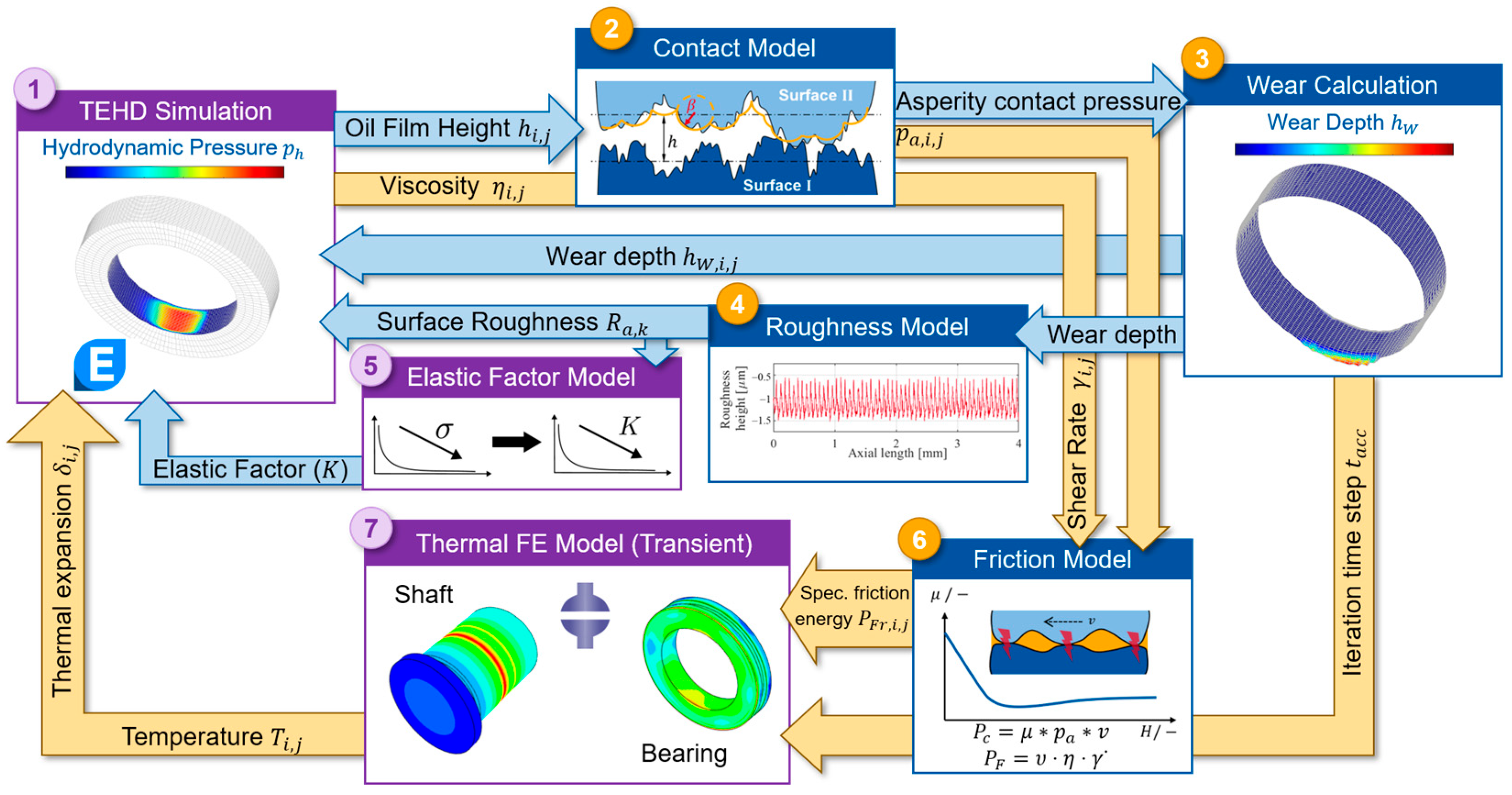
The approach presented in this paper extends an isothermal wear simulation tool developed in previous studies by König [12], Lehmann [10,17] and Decker [18,29]. The isothermal wear simulation is extended by introducing a TEHD model, transient thermal FE models, and an elastic factor model to locally vary the -factor. The iterative process of the extended thermal wear simulation tool is illustrated in Figure 1. In each iteration a TEHD model (1), a contact model (2), a wear calculation tool (3), a surface roughness model (4), an elastic factor model (5), a friction model (6), and a transient thermal FE model (7) are coupled within the simulation framework.
Figure 1.
Workflow of the thermal wear simulation tool with extensions highlighted (violet).
Each iteration of a thermal wear simulation starts with a TEHD simulation (1) performed in commercial software, AVL Excite Power Unit 2022 R1. During the TEHD simulation, the transient Reynolds equation [30] is solved to calculate the pressure distribution between the sliding surfaces at each hydrodynamic (HD) mesh node (). For modelling lubricant flow near the sliding surfaces, the average flow model according to Patir and Cheng [31] is used. In AVL Excite Power Unit, the Greenwood–Tripp contact model [19] is implemented to calculate the asperity contact pressure at each hydrodynamic (HD) mesh node (). Based on the calculated a Matlab R2022b-based wear calculation tool and roughness model determine wear on the macroscopic and microscopic levels, respectively. The theoretical framework of wear calculation tool is described in detail in previous publications by Decker [18] and Lehmann [10]. The roughness model used to update the surface roughness during wear was introduced by König, and its theoretical background is presented in their work [12]. As the surface roughness decreases, the characteristic -factor of the used contact model is proportionally updated using the elastic factor model (5). In the wear calculation tool, a wear model is used to calculate locally occurring wear rate. In a previous study using an isothermal wear simulation, Lehmann [17] parametrized different wear models based on experimental data. A comparison showed that the wear law proposed by Lijesh [32] represents sliding bearing run-in behaviour most accurately. This is because the wear model proposed by Lijesh consists of a time-dependent wear degradation coefficient ) which is calculated using Equation (1) below.
The degradation coefficient is calculated using the initial wear rate (), the stationary wear rate after run-in (), the time constant () which characterizes the duration of run-in, and the effective bearing temperature (). Lehmann [17] showed how to parametrize the degradation coefficient based on experimental data. Lijesh describes wear as a thermodynamic degradation process. The basic principle is that frictional sliding is an irreversible dissipative process in which mechanical energy is converted into heat and material degradation. Therefore, wear is related to the entropy generated by frictional dissipation rather than load and sliding distance only. The governing relation of the model links the wear rate () to the entropy generation rate () through a factor in the form of degradation coefficient (). Under frictional sliding, the is expressed as a ratio of the frictional power () and effective bearing temperature (). The local wear rate () is therefore calculated using Equation (2) below.
The calculation of the friction power () is described in detail in Section 2.3. The time step size after each iteration () is derived from calculated maximum wear rate and a predefined iteration step size (). With this approach, maximum wear depth () in each iteration occurs at the node with maximum asperity contact pressure. To account for heat generation, the local total friction power () is calculated using asperity contact pressure (), coefficient of friction (), lubricant shear rate () and dynamic viscosity (). The procedure for calculating the total friction power is described in Section 2.2. Using as the thermal load and as the time step, transient thermal FE simulations are performed to calculate local temperature and local thermal expansion. The resulting local temperature and thermal expansion profiles of the sliding surfaces, along with the updated bearing contour surface roughness and local -factor, are updated in the next iteration and are thus subsequently incorporated in the TEHD simulation. Heat transfer between the sliding surfaces and lubricant is considered in the TEHD simulation through a non-stationary heat balance. This heat balance considers friction losses and heat transfer between sliding surface and lubricant based on material properties and a non-stationary heat transfer coefficient. The temperature- and pressure-dependent change in lubricant viscosity is described by the Vogel–Barus equation shown below.
A more detailed illustration of the theoretical framework of the thermal wear calculation tool is provided in Figure A1 in Appendix A. Subsequent subsections describe the lubricant properties, the sliding bearing test bench, thermal FE model and the elastic factor model.
2.1. Lubricant Properties
The lubricant used is Castrol Optigear CT 320 which is a commercially used synthetic gear oil of ISO VG class 320. The lubricant contains typical gear-oil additives, including antioxidants and anti-wear additives. To model the temperature- and pressure-dependent viscosity change, constants A, B, C required in Equation (3) were derived from experimental measurements on a falling body viscometer. Detailed information on the experimental setup and measurement procedure is provided in previous studies [33]. The resulting values of these constants, together with the temperature- and pressure-dependent parameter α, are summarized in Table 1 below for the lubricant used in this study.
Table 1.
Constants for the Vogel–Barus Equation.
2.2. Sliding Bearing Test Bench
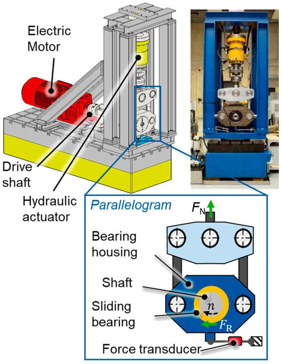
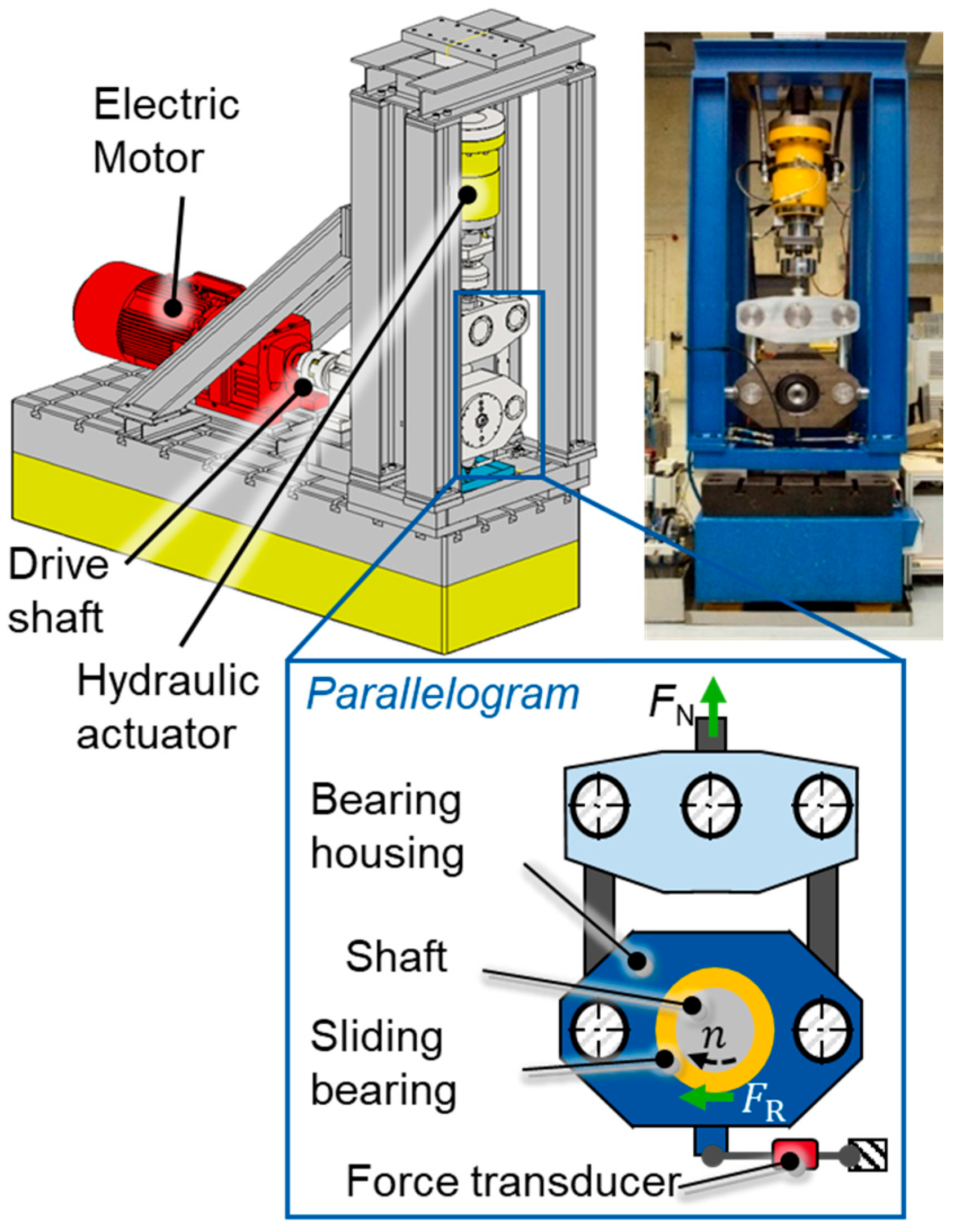
The component-level radial sliding bearing test bench is shown in Figure 2. The shaft is driven by an electric motor and rotates within the inner circumference of the sliding bearing. The bearing is mounted in a housing, which is fixed in a parallelogram to allow radial and small tilting movement which enables the measurement of friction torque. A radial force is applied by the hydraulic actuator which pulls the bearing housing against the rotating shaft. The parallelogram functions as a friction balance, where the friction torque is measured using a force transducer connected through a lever mechanism. The drive shaft is supported by two rolling bearings. Specific pressure loads of up to and sliding speeds between can be achieved on the test bench. The TEHD model shown in Figure 3 includes the shaft, the bearing, and the housing. The EHD joint representing the bearing running surface is discretized into 137 circumferential nodes and 25 axial nodes. Further specifications of the test bench and test pieces are summarized in Table 2 below.
Figure 2.
Radial sliding bearing test bench.
Figure 3.
Components of TEHD model.
Table 2.
Specifications of test bench.
In total, three experiments conducted on the test bench are used to validate the thermal wear simulation. The operating conditions of the validation experiments are summarized in Table 3. At first, a short Experiment 1 was conducted to validate the temperature prediction of the transient thermal model under high friction energy inputs. To validate wear prediction, Experiments 2 and 3 are used which were conducted in a previous study by Decker [18]. All tests were carried out under stationary operating conditions with high loads and low sliding speeds. These operating conditions are particularly relevant for wear in sliding bearings.
Table 3.
Overview of the performed wear validation experiments [18].
During all tests the oil and housing temperatures were controlled using heating cartridges. During Experiments 2 and 3, the bearing temperature was measured with a PT100 thermocouple from OTOM GmbH placed at the centre of the bearing load zone, 3 mm below the running surface. For a comprehensive validation of the transient thermal models, temperature measurement for Experiment 1 was performed using 24 high-precision digital temperature sensors as applied and explained by Baszenski [34]. The 24 measurement positions are oriented in loaded bearing half between , with an angular spacing of . The tests were started once the bearing temperature reached the oil and housing temperatures. The test specimens were subjected to tactile measurements before and after the test. The bearing contour and roughness profiles were recorded at several angular positions. The initial roughness profiles served as input for the TEHD model at the start of the wear simulation. The bearing contour measurements before and after the test were used to determine the wear volume generated. The procedure for evaluating wear volume from experimental data is described in detail in previous studies [17,18]. The experimental results from these conducted tests are discussed in Section 3.
2.3. Thermal FE Modelling
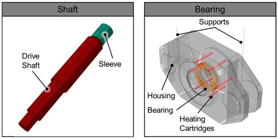
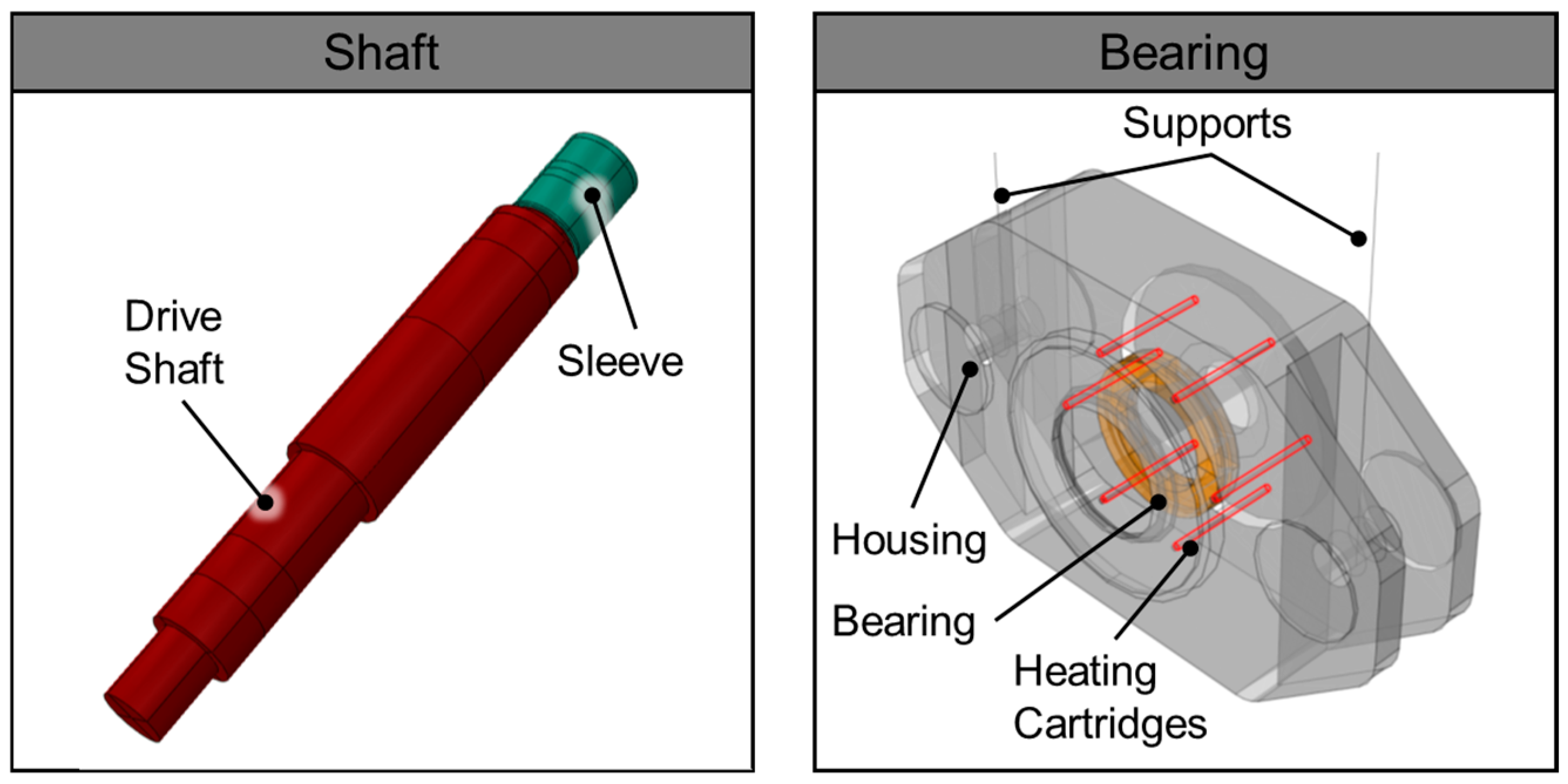
The thermal FE models used in this study were developed in commercial FE software, Abaqus CAE 2019. Separate models were created for the shaft and bearing-housing assembly. Figure 4 illustrates the components included in the thermal FE models.
Figure 4.
Components of the thermal FE models for shaft (left) and housing (right).
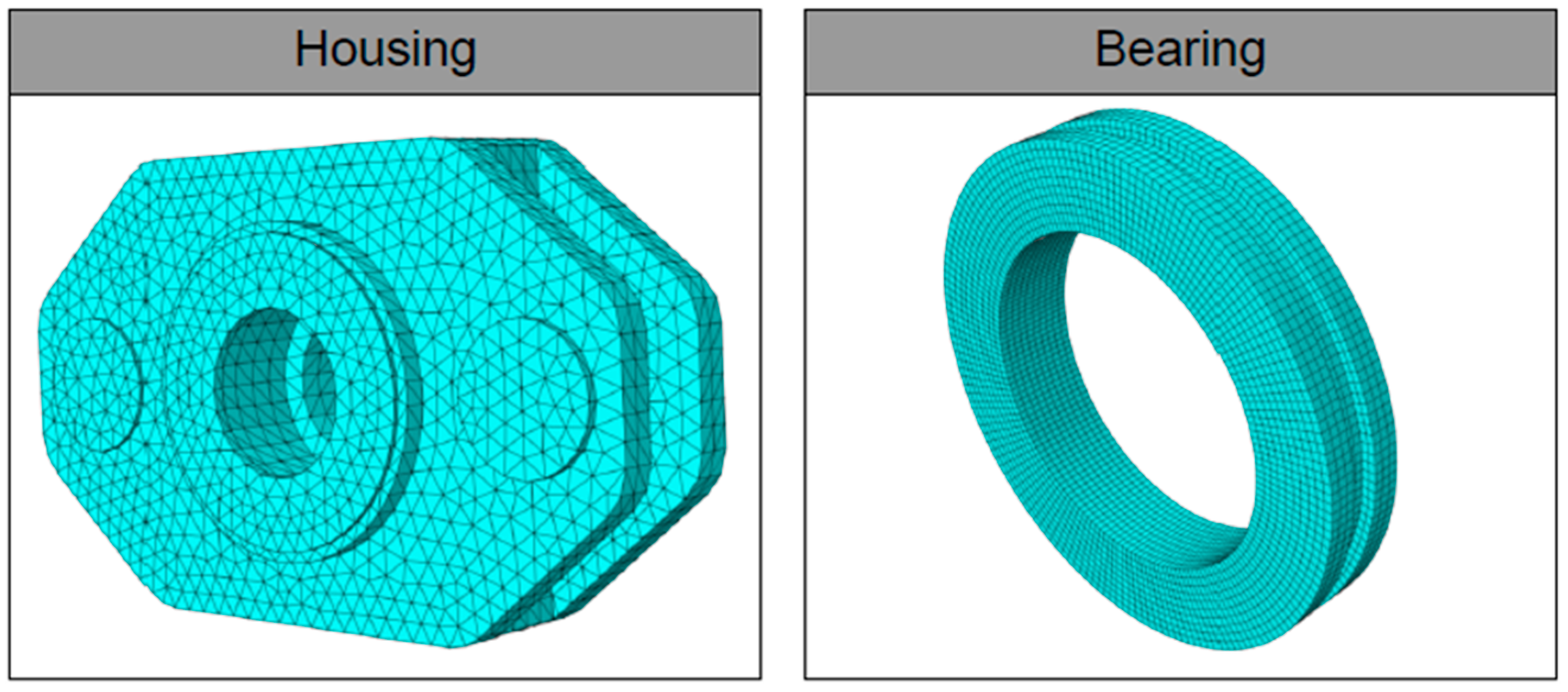
The housing model includes the bearing housing, sliding bearing, heating cartridges, and housing supports. The heating cartridges are used to reproduce the thermal boundary conditions of the test bench and are therefore modelled as heat sources in the thermal FE simulations. The bearing is assembled in the housing with its outer circumference tied to the inner cylindrical surface of the housing. The shaft model contains the complete test-bench shaft and a sleeve mounted on the shaft without allowing relative motion (tie constraint). Thermal calculations are performed using simulations to account for interaction between temperature and thermal expansion (coupled temperature–displacement simulations). The free surfaces of the housing are subject to natural convection by air with heat transfer coefficients between [23]. The thermal boundary conditions for heating (cartridges) and cooling (convection) were validated in a previous study by the authors [23]. The validation was performed by measuring housing surface temperatures with a thermal camera and comparing them with transient thermal simulations [23]. The FE meshes of the bearing and housing are shown in Figure 5.
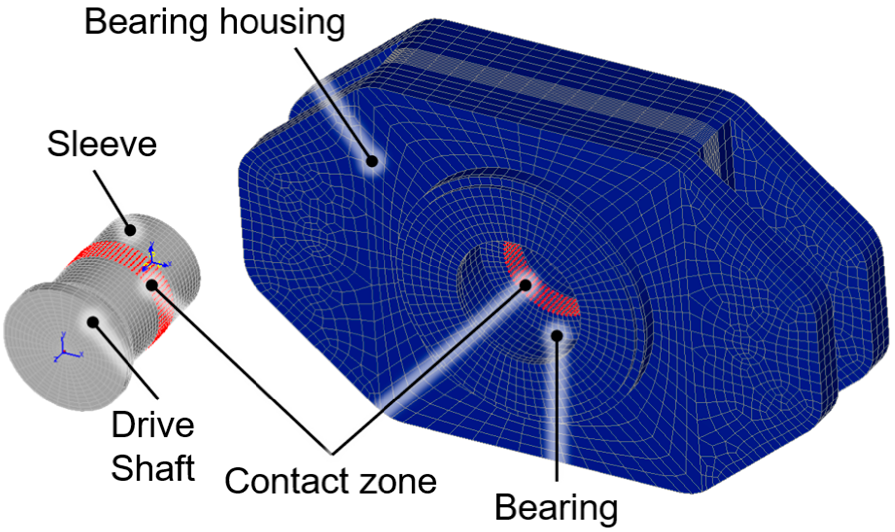
Figure 5.
FE meshes of housing (left) and sliding bearing (right).
Linear hexahedral element types are used to model the bearing, heating cartridge, shaft and sleeve, whereas the housing is modelled using linear tetrahedral elements. The housing supports are modelled using one-dimensional elements to improve computational efficiency while still representing the mechanical constraints. Before the first iteration, the heating phase of the test bench is simulated using an FE model. This ensures that the initial TEHD simulation starts with the temperature and thermal expansion profiles in preheated operating state. Once the wear simulation starts, each TEHD simulation is followed by a thermal FE simulation to account for local frictional heating in the bearing. Each FE simulation begins with the temperature and thermal expansion fields obtained at the end of the previous wear iteration. This enables simulation of the transient thermal behaviour during wear progression. The total friction power () results from heat generated by mixed friction ) and fluid friction (). Equation (4) below shows the calculation of .
The first term represents mixed friction power, while the second term represents fluid friction power. All variables except the sliding speed () are calculated locally, enabling spatially resolved frictional heating. The coefficient of friction () is determined using the approach proposed by Offner and Knaus [35]. The Coulomb’s boundary friction coefficient () required for calculating , is set to which is typical for bronze-steel material pairs [36,37,38]. Only a fraction of the mixed friction power is applied as thermal load to the bearing. Experimental investigations by Shakhvorostov [39] showed at least 70% of the friction power is converted into heat during mixed friction. The remaining part contributes to generation of wear and material change [39]. The local dynamic viscosity () and shear rate () are obtained from the TEHD simulation. The resulting friction power is distributed between the shaft and the bearing according to their thermal conductivities [24]. Due to the rotational motion of the shaft, the generated heat is averaged over the shaft circumference [23,24]. The thermal model was validated for bearing temperature calculation in both temporal and spatial resolution by the author in a previous study [23]. In this paper, the validated thermal model is used to improve prediction of wear volume and run-in behaviour in sliding bearings. The next subsection introduces the improved modelling of contact evolution using the elastic factor model.
2.4. Elastic Factor Model
The elastic factor model is used to locally vary the -factor in asperity contact calculation with the Greenwood–Tripp model [19] during a wear simulation. The introduction of the elastic factor model helps improve the prediction of contact condition evolution during wear progression. The Greenwood–Tripp contact model is characterized by the elastic -factor, which combines three surface roughness parameters as shown in Equation (5).
The composite summit roughness () can be reliably obtained from 2D tactile measurements. In contrast, determining the summit radius () and asperity peak density () from practical relevant 2D tactile measurements is very difficult [40]. Previous studies have also shown that deriving these values reliably from 3D measurements is challenging. This is due to their high sensitivity to measurement resolution and evaluations methods [41,42]. Therefore, commercial software such as AVL Excite Power Unit commonly uses a constant -factor to parametrize the contact model. However, accurate modelling of sliding bearing run-in requires the -factor to vary with the evolving surface roughness.
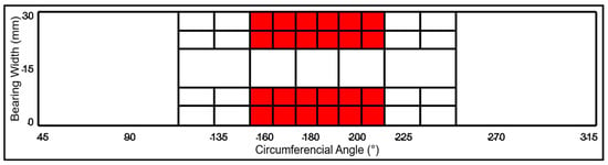
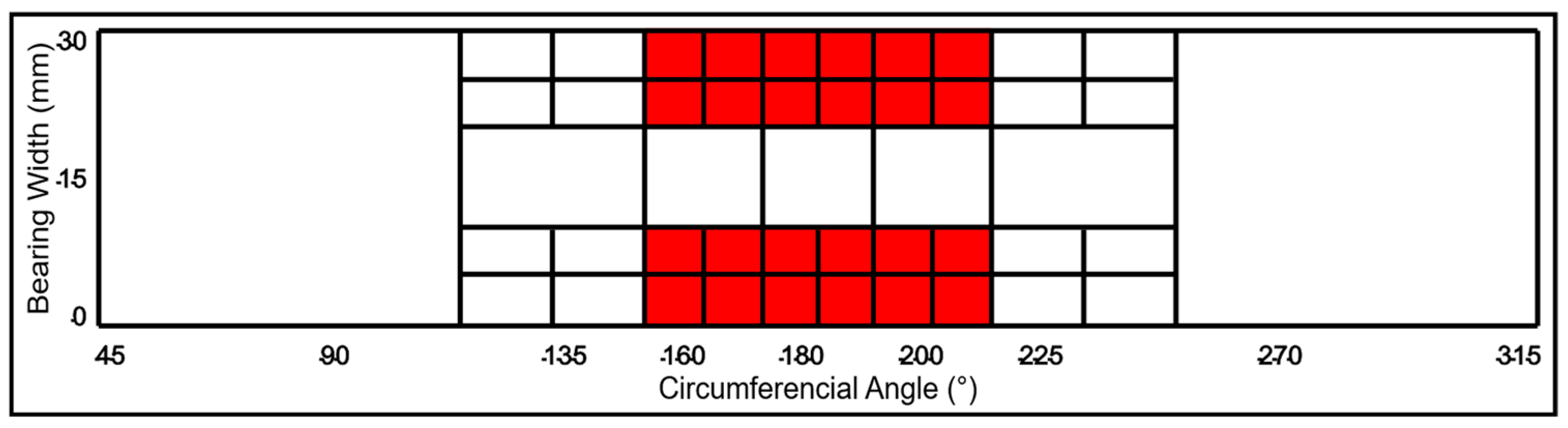
In this study, the initial value of -factor at the start of the wear simulation is defined using a TEHD simulation together with the measured friction torque from the test bench. The surface roughness measured before the test is used as input for the TEHD simulation. These measured roughness values are assigned locally to the bearing surface through contact patches in the simulation. Figure 6 illustrates the discretization of the bearing surface into contact patches defined in the TEHD model. During the wear simulation, the roughness values are updated locally at the patches where wear occurs.
Figure 6.
Bearing surface contact patches in the TEHD model in AVL Excite Power Unit.
The area highlighted in red represents the expected contact zone of the radial sliding bearing. Therefore, the patches in this region are discretized more finely to improve spatial resolution of roughness parameters. For each validation experiment and corresponding bearing roughness, an appropriate initial -factor must be defined. To determine this value, a trial-and-error approach using TEHD simulations was performed. The value at which the simulated friction torque matches the experimental measurement is defined as the reference elastic factor (). This value is assigned to the patch with the highest composite summit roughness (), since is proportional to (Equation (5)). In this approach it is assumed and remain unchanged and hence do not influence . Experimental investigations by König [12] showed that remains nearly constant during run-in, while changes only slightly. Based on this observation, the -factor values for the remaining patches () are calculated from the corresponding composite summit roughness (), using a proportionality exponent d as shown in Equation (6) below.
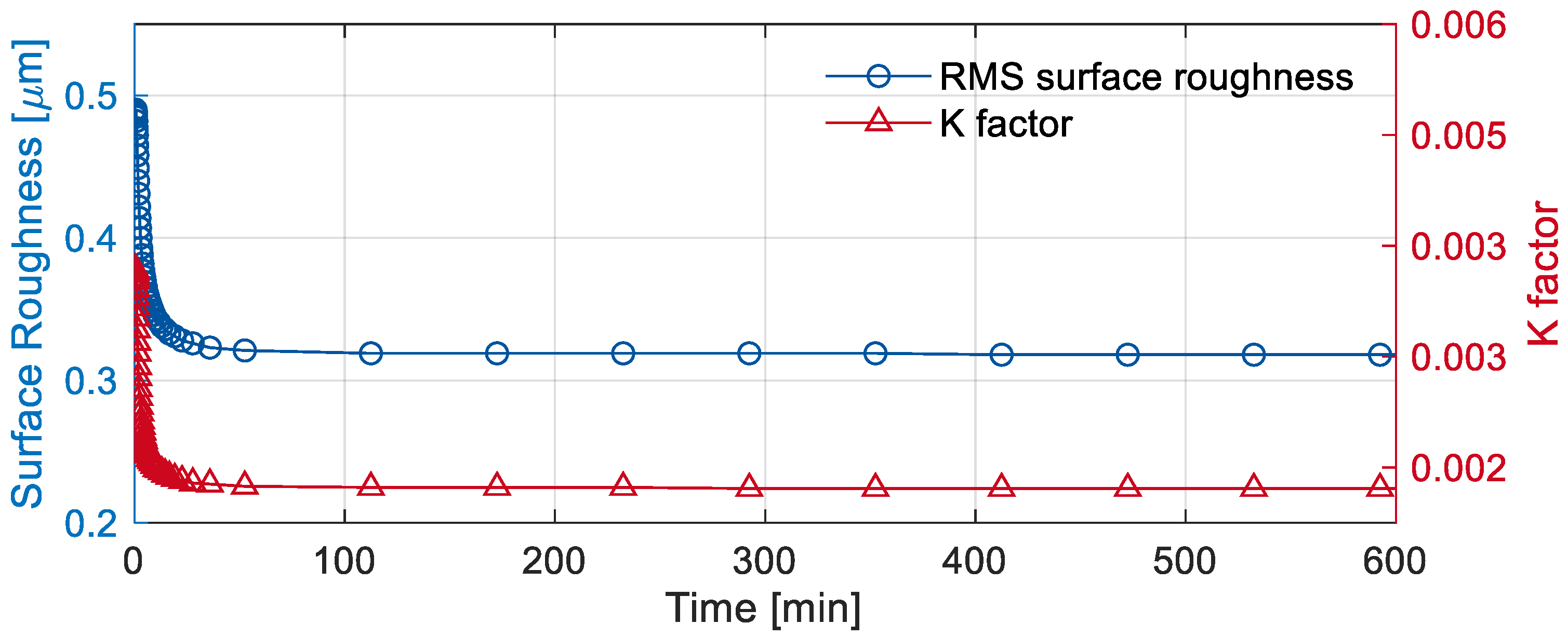
Here, which represents the proportionality between and is derived from Equation (5). With this approach the contact model is parametrized to match the peak friction torque measured at the start of the experiment. The resulting evolution of friction torque over time is then compared with experimental measurements for validation. During the wear simulations, the local -factors () are updated in proportion to reduction in corresponding surface roughness (). Figure 7 illustrates the evolution of surface roughness and the -factor during a wear simulation for Experiment 2. As an example, the evolution is shown for one surface patch located in the contact zone.
Figure 7.
Evolution of surface roughness and elastic -factor for a surface patch during a wear simulation.
This approach is intended to improve the representation of bearing contact evolution during run-in wear. The prediction accuracy of run-in behaviour is evaluated by comparing the friction torque evolution and bearing contour measurements from simulations with experiments in the next section.
3. Results and Discussion
In this section, the validation results of the proposed simulation approach are presented. The focus lies on prediction of run-in wear characteristics, thermal behaviour and wear generation. For this purpose, thermal wear simulation results are compared with experimental data obtained under operating conditions listed in Table 3. Wear is calculated using the Lijesh wear model [32]. The required parameters such as initial wear rate and stationary wear rate were previously parametrized by Lehmann [17] for identical operating conditions on the same test bench. For the simulations performed in this study, the corresponding parametrization from Lehmann [17] is adopted.
3.1. Validation of Temperature Prediction
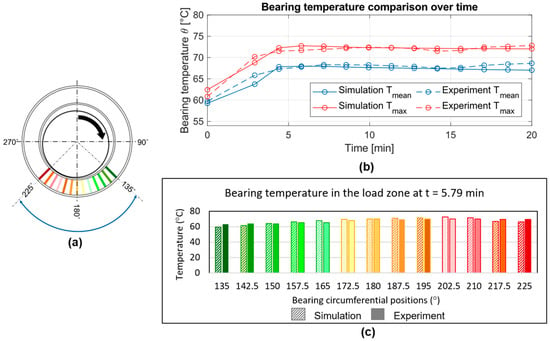
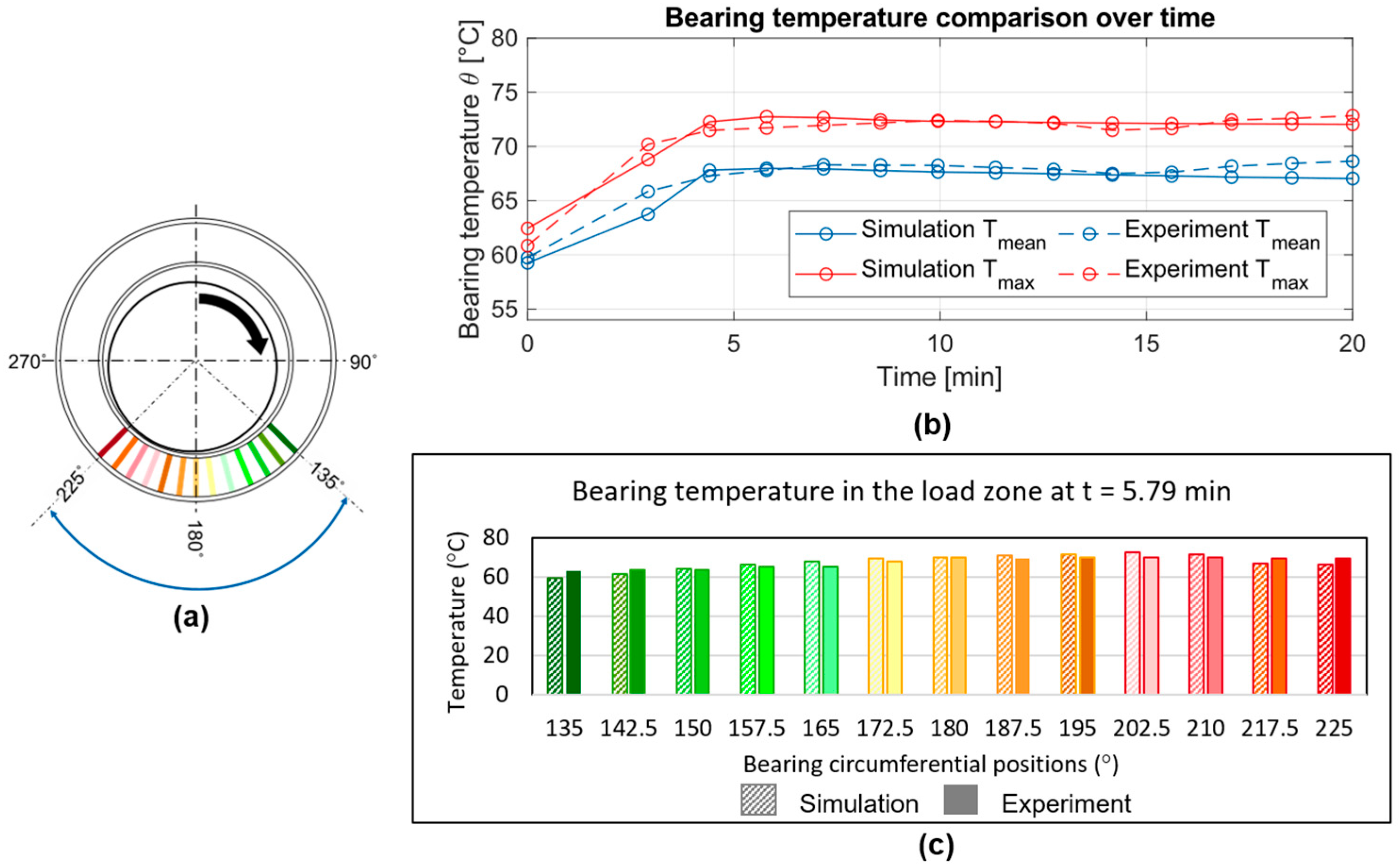
To validate the transient thermal FE model, the predictions of bearing temperature over time and along the bearing circumference are evaluated. For this purpose, temperature measurements from Experiment 1 are compared with the corresponding simulation results, as shown in Figure 8.
Figure 8.
(a) Temperature sensor orientation in Experiment 1 and comparison between experiment and simulations for (b) mean and maximum local bearing temperatures over time, and (c) temperature distribution over bearing circumference at
Figure 8a shows the positions of the temperature sensors in the bearing load zone (–). The temporal evolution of the mean bearing temperature in the load zone and maximum local temperature () is presented in Figure 8b. The comparison results in a maximum absolute error of , indicating high accuracy in predicting the transient bearing temperature. To evaluate the spatial prediction, the circumferential temperature distribution from experiments and simulations is compared at min, as shown in Figure 8c. The maximum deviation is , demonstrating the ability of the thermal model to capture local temperature variations. Based on these comparisons, the introduced thermal FE model accurately predicts both the temporal and spatial evolution of bearing temperature.
3.2. Transient Wear Characteristics
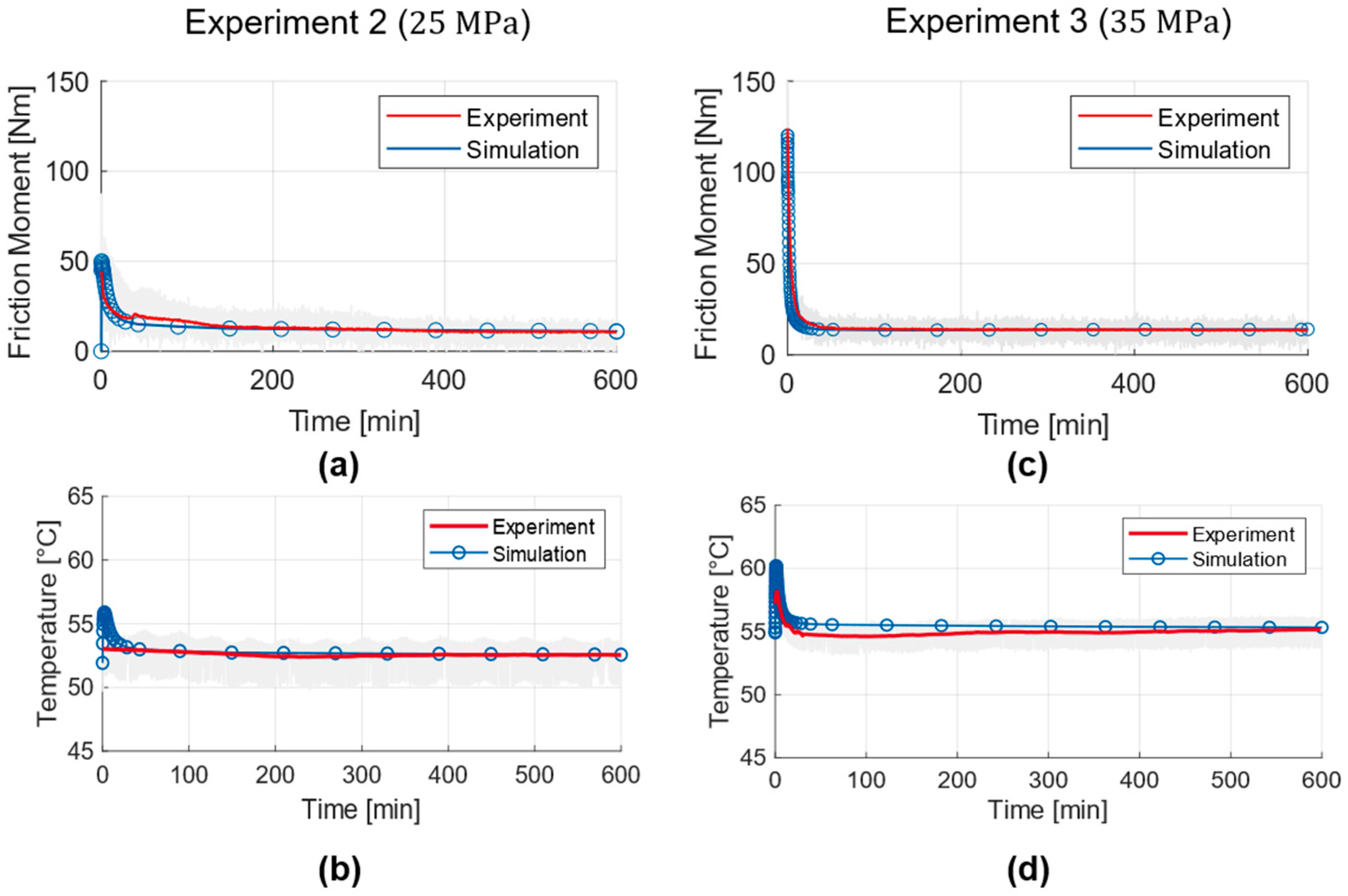
Sliding bearing run-in is characterized by a reduction in surface roughness and wear intensity over time. On the test bench, run-in behaviour is evaluated using the measured friction torque and bearing temperature. An initially high wear rate results from increased friction, which heads to higher friction torque and temperature. As surface roughness decreases, the wear intensity declines, and both friction torque and temperature are reduced. Once a steady wear rate is reached, these values remain nearly constant. The thermal wear simulation helps capture this run-in behaviour through the evolution of friction torque and bearing temperature. Figure 8 compares simulated and experimental results for friction torque and bearing temperature for Experiments 2 and 3 (see Table 3).
During the wear simulations, the friction torque and bearing temperature reach maximum peaks in the initial iterations. Their subsequent evolution is similar to the reduction in surface roughness shown in Figure 7. The linear wear phase, which is after run-in, is indicated by a quasi-stationary friction torque. This is achieved after approximately 100 min in Experiment 2 and 50 min in Experiment 3. The difference in the initial friction torque peak magnitude between the two experiments is primarily attributed to the higher specific pressure in Experiment 3 compared with Experiment 2. In addition, the bearing used in Experiment 3 has a slightly higher surface roughness () than the bearing in Experiment 2 (). The combination of higher specific pressure and greater surface roughness increases asperity interactions in Experiment 3, resulting in a more pronounced friction-torque peak. The thermal wear simulation captures the friction torque evolution during run-in accurately. The maximum error is 6 Nm for Experiment 2 and 4 Nm for Experiment 3. In simulations, the development of mean bearing temperature correlates with the friction torque evolution. However, the measured temperature rise in Experiment 2 is negligible compared to Experiment 3. This indicates that the generated frictional heat in Experiment 2 is low and is effectively dissipated through heat distribution in the bearing and convection to lubricant. It should also be noted that the temperature measurements contain some noise, indicating signal discrepancies in the range of . Due to the negligible temperature rise in Experiment 2, the prediction error is higher () compared to Experiment 3 (). Overall, the results in Figure 9 show good agreement between simulations and experiments. The high-fidelity thermal and contact modelling enables accurate prediction of run-in wear characteristics in sliding bearings. The next subsection evaluates the accuracy of wear prediction using the thermal wear simulation.
Figure 9.
Evolution of friction torque and bearing temperature over time for Experiment 2 (a,b) and Experiment 3 (c,d).
3.3. Validation of Wear Prediction
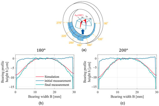
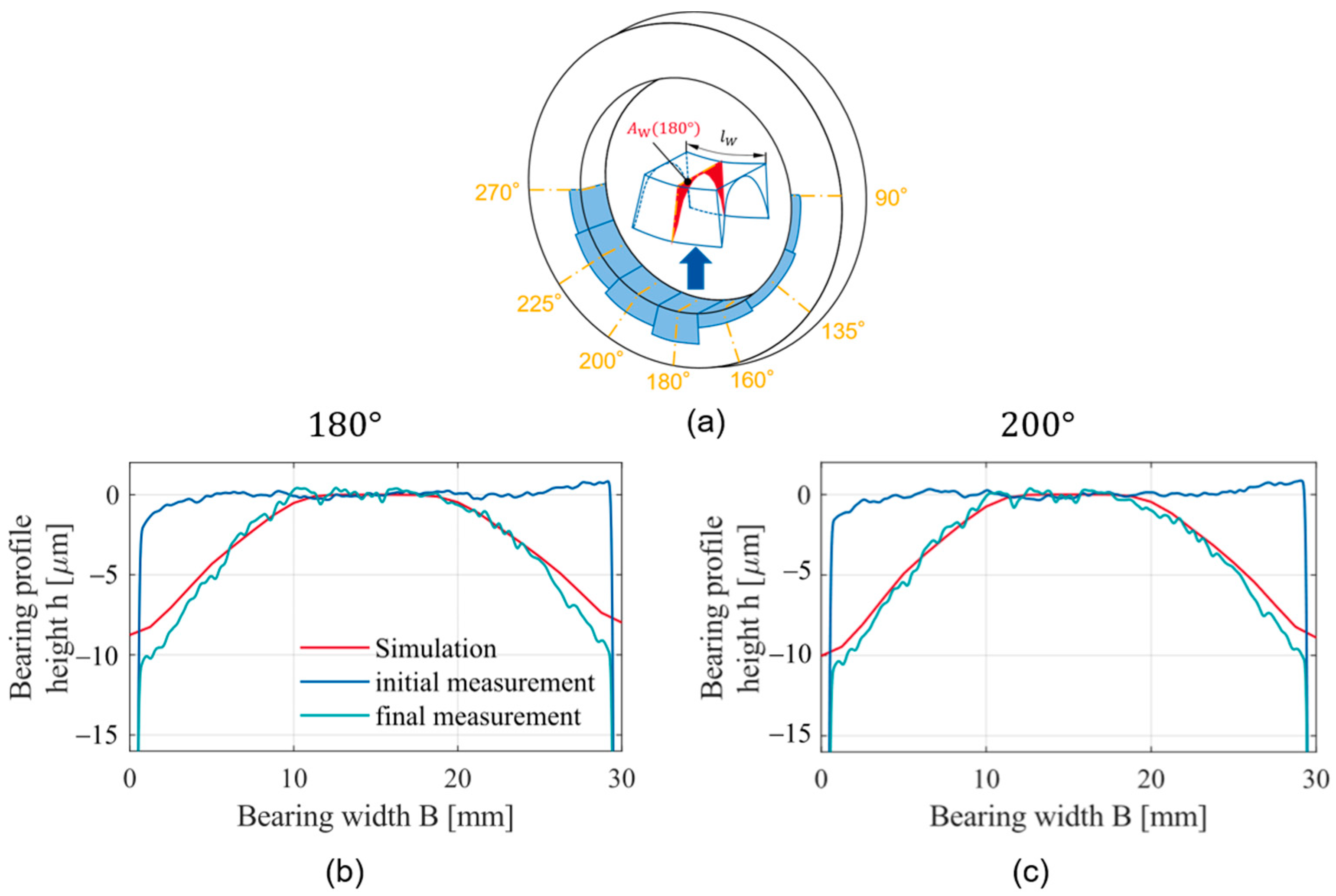
Previous attempts to validate the wear simulation for predicting wear generation were reported by Decker [18]. In that study, only a comparison of bearing contour profiles between simulations and experiments was made. However, the validation showed an error in maximum wear depth of around 35% and no validation of wear volume was presented. One possible reason for this deviation may be the neglection of thermal effects in the simulations. In the present study, the thermal wear simulation is validated by comparing predicted bearing contours and wear volume with experimental evaluations. Figure 10 below illustrates the bearing circumferential positions for tactile measurements and shows a comparison between experimentally measured bearing contour and simulated bearing contour after wear for Experiment 3.
Figure 10.
(a) Bearing circumferential positions for tactile measurements, and comparison of bearing contour between Experiment 3 and corresponding wear simulation at 180° (b) and 200° (c).
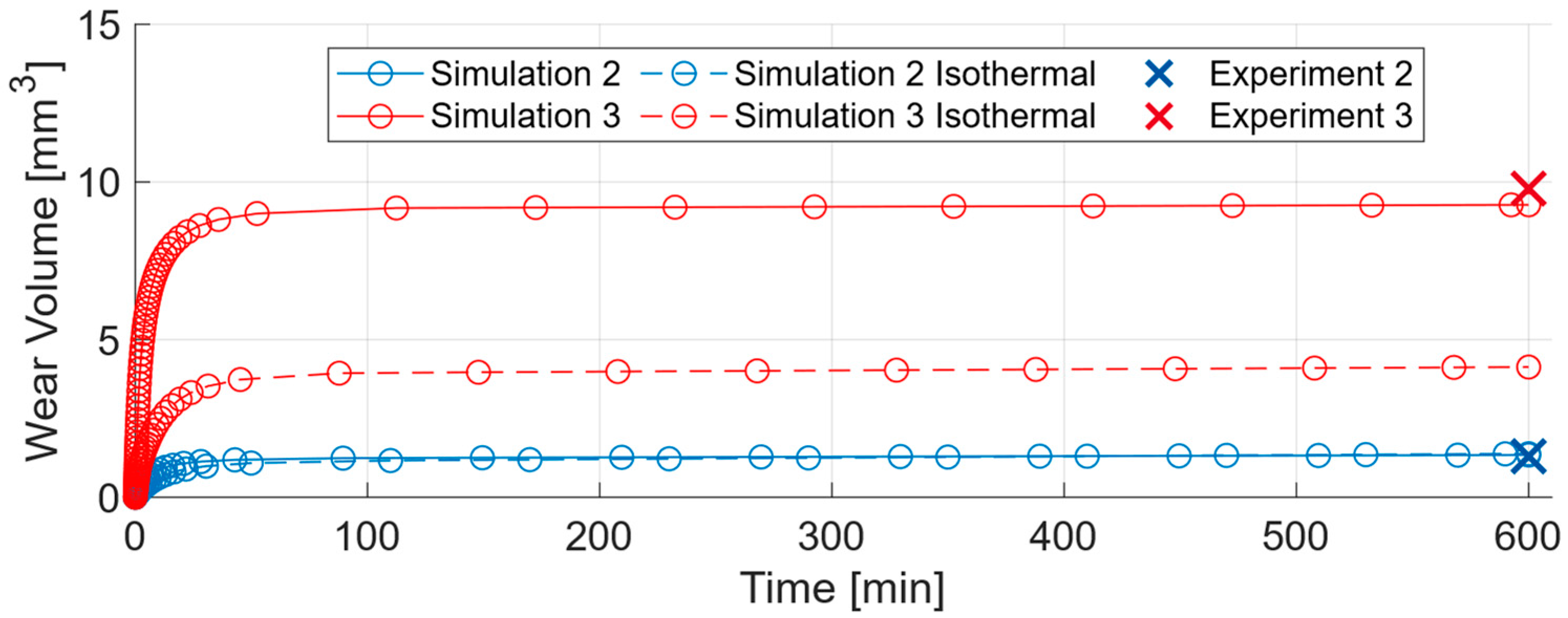
The overlap of the initial and final tactile measurements clearly illustrates the axial wear distribution along the bearing width. The wear depth is highest at the edge and decreases towards the bearing centre which is typical for radian sliding bearings [10,17]. The final measured contour is compared with the simulated worn profile for validation. The axial wear distribution is reproduced well by the thermal wear simulations. The maximum relative error is 13%, corresponding to an absolute deviation of 1.32 µm between the simulated maximum wear depth (8.76 µm) and experimental measurement (10.08 µm). The bearing wear volume is obtained by integrating the 2D wear contours over the bearing surface area [17,18]. Therefore, accurate contour prediction at each angular position leads to reliable wear volume estimation. Figure 11 compares the wear volumes obtained from thermal and isothermal wear simulations and experiments.
Figure 11.
Comparison of wear volume generated between thermal wear simulation, isothermal wear simulation and experiments.
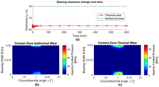
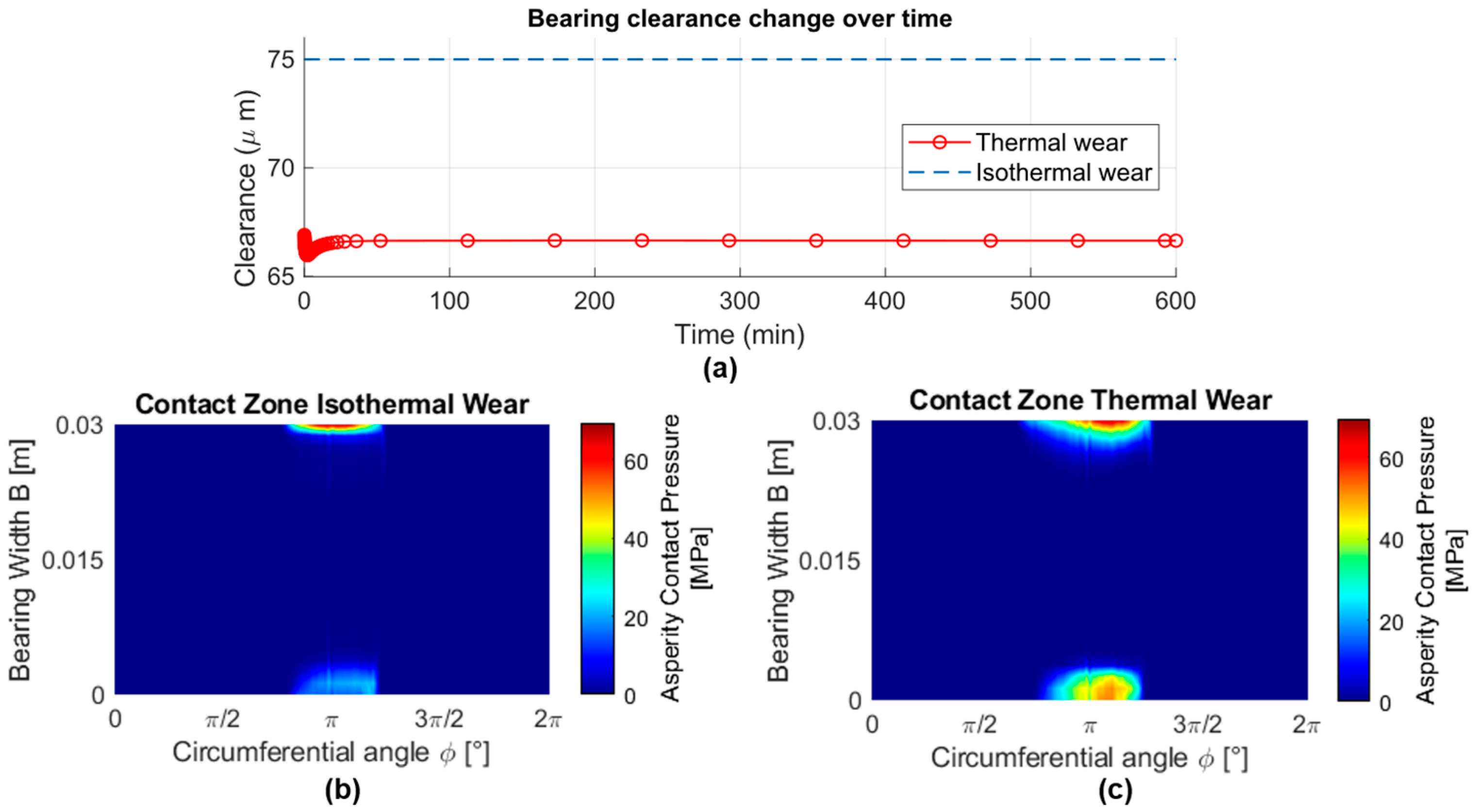
The transient development of wear volume in the simulations reflects the duration of the run-in phase of the sliding bearing as seen in Figure 9. A high initial wear rate causes a rapid increase in wear volume. After run-in is completed, the wear volume remains relatively unchanged. The difference in predicted wear volume between the isothermal and thermal wear simulations is significantly larger for Simulation 3 than for Simulation 2. This significant difference arises because isothermal simulations neglect bearing clearance change caused by thermal effects. To illustrate this, Figure 12 below compares the temporal evolution of bearing radial clearance in the isothermal and thermal wear simulations, together with the resulting contact zones at .
Figure 12.
(a) Comparison of temporal evolution of bearing clearance between the isothermal and thermal wear simulations for Experiment 3; asperity contact pressure distribution at for (b) isothermal wear simulation and (c) thermal wear simulation.
Due to the neglection of temperature rise in the isothermal simulation, thermal expansion does not occur and the bearing clearance remains unchanged (Figure 12a). In contrast, the thermal simulation predicts a consistently lower clearance, as local temperature rise and the resulting thermal expansion are considered over time (Figure 12a). Local thermal expansion of the sliding surfaces widens the bearing contact zone in both the circumferential and axial directions, as shown in Figure 12c. As a result, the worn surface area increases, leading to a larger generated wear volume in the thermal wear simulation compared with the isothermal simulation. For Experiment 2, the difference between both simulation approaches is small, since the bearing temperature changes only slightly (Figure 9). Since tactile measurements were only made at the start and end of the tests, comparisons between simulations and experiments are possible only at . The prediction errors in wear volume are 3.08% for Thermal Simulation 2 and 6.73% for Thermal Simulation 3. One source of error is the neglect of the measured bearing contour in TEHD simulations. In the present approach, the wear simulations start from a perfectly cylindrical bearing contour. This simplification affects the local wear-depth prediction as the predicted location of wear may deviate from reality. Incorporating the measured bearing contour in TEHD simulations would require resolving and meshing local asperity features on the bearing surface to ensure simulation convergence [43,44]. This would significantly increase the mesh density and computational effort. For practical applications, such computationally intensive simulations would be unsuitable. Despite this limitation, the prediction accuracy of wear volume improves significantly with the introduction of transient thermal FE modelling. This improvement is particularly good for Experiment 3, where the prediction accuracy increases by 37% when thermal effects are included in wear simulation.
4. Conclusions
In heavy-duty applications, sliding bearings can experience high loads at low speeds, leading to mixed friction and consequently wear. To understand this wear behaviour, iterative wear simulations are used to model wear-induced changes in sliding bearings. During wear progression, sliding bearings undergo surface topography changes and thermal changes due to temperature rise. Although existing wear simulations capture surface topography changes, they fail to capture the effect of these changes on the parameters of contact models, particularly the Greenwood–Tripp model. Next to that, transient thermal effects are neglected. These limitations reduce the accuracy of predicting the wear evolution over time. To address this research gap, an isothermal wear simulation tool is extended for thermal wear calculation in this paper. The novelty lies in extending the existing wear simulation by incorporating transient thermal effects and improved contact modelling. Transient thermal effects are considered by integrating thermal FE modelling in the wear simulation. The FE models help capture local and transient changes in temperature and thermal expansion on the sliding surfaces. Asperity contact calculation using the Greenwood–Tripp model is improved by locally varying the elastic factor () over time. This local and temporal variation in -factor helps represent the effect of surface topography changes in asperity contact calculation. The extension of the wear simulation helps capture changes in bearing contact conditions due to thermal effects and due to changing surface topography.
The proposed extensions enable a more accurate prediction of transient run-in characteristics and wear volume in sliding bearings. These characteristics are evaluated using simulation outputs such as friction torque, bearing temperature, worn bearing contour, and wear volume. The average prediction error across these parameters remains below 5%, indicating good agreement between simulations and experiments. Overall, the thermal wear simulation improves wear volume prediction by around 37% in comparison to isothermal wear simulations.
The present study focuses on modelling abrasive wear in sliding bearings. In these processes limited thermal energy is generated as seen by the limited temperature increase over time. Therefore, the proposed methodology should be further validated with higher thermal inputs most likely leading to adhesive wear and more diverging temperatures. Adhesive wear can lead to bearing overheating and therefore damage. Future works should therefore apply the thermal wear simulation to investigate overheating and adhesive failure mechanisms in sliding bearings.
Author Contributions
Conceptualization, A.K.; methodology, A.K., A.D. and M.B.; software, A.K.; validation, A.K. and A.D.; formal analysis, A.K.; investigation, A.K.; resources, A.K., T.B. and M.B.; data curation, A.K., T.B. and M.B.; writing—original draft preparation, A.K. and M.B.; writing—review and editing, M.L. and B.L.; visualization, A.K. and A.D.; supervision, G.J., B.L. and M.L.; project administration, G.J.; funding acquisition, G.J. All authors have read and agreed to the published version of the manuscript.
Funding
This research was funded by German Federal Ministry of Economic Affairs and Energy (grant number 03EE3054A), and by the Deutsche Forschungsgemeinschaft (DFG, German Research Foundation; grant numbers 466775494 and 441853410).
Data Availability Statement
The data presented in this study are available on request from the corresponding author.
Conflicts of Interest
The authors declare no conflicts of interest.
Abbreviations
The following abbreviations are used in this manuscript:
| HD | Hydrodynamic |
| EHD | Elasto-hydrodynamic |
| TEHD | Thermo-elastohydrodynamics |
| FE | Finite element |
| ISO | International Standards Organization |
| VG | Viscosity grade |
| 2D | Two-dimensional |
| 3D | Three-dimensional |
Appendix A
The theoretical flow process of the proposed thermal wear calculation tool is presented in the Figure A1 below. The new integrated elements under focus in this study are highlighted in violet. The definition of symbols used in Figure A1 can be referred to in Table A1 below.
Figure A1.
Detailed theoretical flow process of the thermal wear calculation tool.
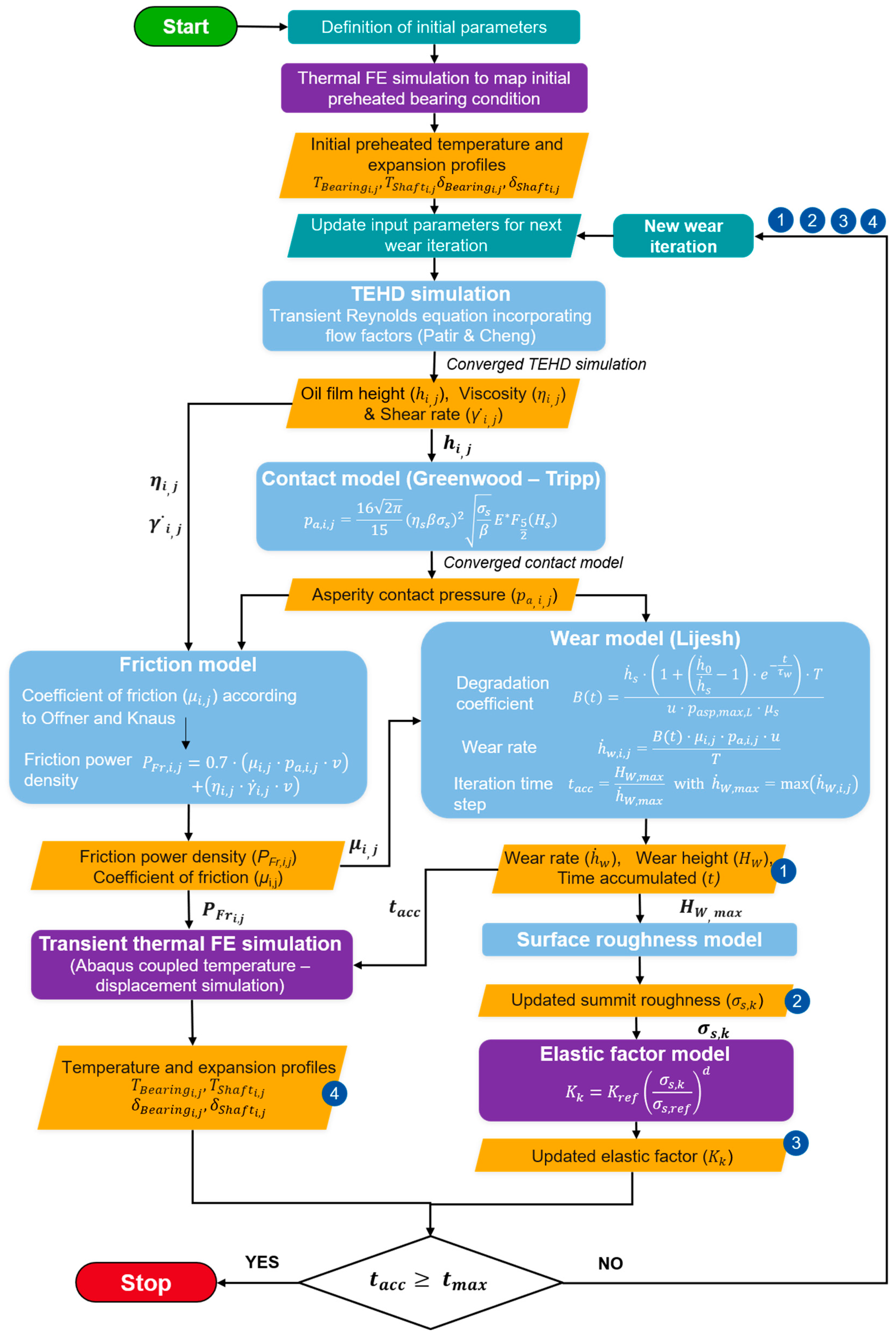
Table A1.
List of symbols from Figure A1.
References
- Sander, D.E.; Allmaier, H.; Priebsch, H.H.; Reich, F.M.; Witt, M.; Füllenbach, T.; Skiadas, A.; Brouwer, L.; Schwarze, H. Impact of high pressure and shear thinning on journal bearing friction. Tribol. Int. 2015, 81, 29–37. [Google Scholar] [CrossRef] [Scilit]
- Knauder, C.; Allmaier, H.; Sander, D.; Salhofer, S.; Reich, F.; Sams, T. Analysis of the Journal Bearing Friction Losses in a Heavy-Duty Diesel Engine. Lubricants 2015, 3, 142–154. [Google Scholar] [CrossRef] [Scilit]
- Lucassen, M.; Jacobs, G.; Lehmann, B. Efficient dynamic simulations of planetary journal bearings in wind turbine gearboxes. Forsch. Ingenieurwesen 2025, 89, 20. [Google Scholar] [CrossRef] [Scilit]
- Hagemann, T.; Ding, H.; Radtke, E.; Schwarze, H. Operating Behavior of Sliding Planet Gear Bearings for Wind Turbine Gearbox Applications—Part I: Basic Relations. Lubricants 2021, 9, 97. [Google Scholar] [CrossRef] [Scilit]
- Gilges, M.; Saleh, A.; Bekker, A.; Jain, M.; Lehmann, B.; Jacobs, G. Influence of Propeller–Ice Loads on the Wear Development in Stern Tube Bearings of Marine Propulsion Systems and Identification of Critical Operating Conditions. J. Offshore Mech. Arct. Eng. 2024, 146, 061602. [Google Scholar] [CrossRef] [Scilit]
- Vartdal, B.J.; Gjestland, T.; Arvidsen, T.I. Lateral Propeller Forces and their Effects on Shaft Bearings. In Conference Proceedings of First International Symposium on Marine Propulsors; Koushan, K., Steen, S., Eds.; MARINTEK (Norwegian Marine Technology Research Institute): Trondheim, Norway, 2009. [Google Scholar]
- Santos, N.D.S.A.; Roso, V.R.; Faria, M.T.C. Review of engine journal bearing tribology in start-stop applications. Eng. Fail. Anal. 2020, 108, 104344. [Google Scholar] [CrossRef] [Scilit]
- Vencl, A.; Rac, A. Diesel engine crankshaft journal bearings failures: Case study. Eng. Fail. Anal. 2014, 44, 217–228. [Google Scholar] [CrossRef] [Scilit]
- Eyre, T.S. Wear characteristics of metals. Tribol. Int. 1976, 9, 203–212. [Google Scholar] [CrossRef] [Scilit]
- Lehmann, B.; Trompetter, P.; Guzmán, F.G.; Jacobs, G. Evaluation of Wear Models for the Wear Calculation of Journal Bearings for Planetary Gears in Wind Turbines. Lubricants 2023, 11, 364. [Google Scholar] [CrossRef] [Scilit]
- Bartel, D.; Bobach, L.; Illner, T.; Deters, L. Simulating transient wear characteristics of journal bearings subjected to mixed friction. Proc. Inst. Mech. Eng. Part J J. Eng. Tribol. 2012, 226, 1095–1108. [Google Scholar] [CrossRef] [Scilit]
- König, F. Prognose des Verschleißverhaltens Ölgeschmierter Gleitlager im Mischreibungsbetrieb. Ph.D Thesis, Rheinisch-Westfälischen Technischen Hochschule (RWTH) Aachen, Aachen, Germany, 2020. [Google Scholar]
- Sander, D.E.; Allmaier, H.; Priebsch, H.H.; Witt, M.; Skiadas, A. Simulation of journal bearing friction in severe mixed lubrication—Validation and effect of surface smoothing due to running-in. Tribol. Int. 2016, 96, 173–183. [Google Scholar] [CrossRef] [Scilit]
- Khonsari, M.M.; Ghatrehsamani, S.; Akbarzadeh, S. On the running-in nature of metallic tribo-components: A review. Wear 2021, 474–475, 203871. [Google Scholar] [CrossRef] [Scilit]
- Saleh, A.; Gilges, M.; Lehmann, B.; Jacobs, G. (Eds.) Assessing the Influence of the Running-in Phase in Ship’s Stern Tube Bearings on Wear Development During Ice Collision Loads; Department of Marine Technology, Norwegian University of Science and Technology: Trondheim, Norway, 2024. [Google Scholar]
- König, F.; Ouald Chaib, A.; Jacobs, G.; Sous, C. A multiscale-approach for wear prediction in journal bearing systems—From wearing-in towards steady-state wear. Wear 2019, 426–427, 1203–1211. [Google Scholar] [CrossRef] [Scilit]
- Lehmann, B.; Jacobs, G.; Lucassen, M.; Decker, T.; Khare, A.; Bosse, D.; Wang, S. Tool chain for wear prediction of journal bearings in planetary gears in wind turbines. In Bearing World Journal; Poll, G., Pinnekamp, B., Kunze, C., Eds.; Forschungsvereinigung Antriebstechnik e.V (FVA): Frankfurt am Main, Germany, 2024; pp. 63–76. [Google Scholar]
- Decker, T.; Jacobs, G.; Graeske, C.; Röder, J.; Lucassen, M.; Lehmann, B. Multiscale-simulation method for the wear behaviour of planetary journal bearings in wind turbine gearboxes. J. Phys. Conf. Ser. 2024, 2767, 52012. [Google Scholar] [CrossRef] [Scilit]
- Greenwood, J.A.; Tripp, J.H. The Contact of Two Nominally Flat Rough Surfaces. Proc. Inst. Mech. Eng. 1970, 185, 625–633. [Google Scholar] [CrossRef] [Scilit]
- Prölß, M.; Schwarze, H.; Hagemann, T.; Zemella, P.; Winking, P. Theoretical and Experimental Investigations on Transient Run-Up Procedures of Journal Bearings Including Mixed Friction Conditions. Lubricants 2018, 6, 105. [Google Scholar] [CrossRef] [Scilit]
- Beheshti, A.; Khonsari, M.M. An engineering approach for the prediction of wear in mixed lubricated contacts. Wear 2013, 308, 121–131. [Google Scholar] [CrossRef] [Scilit]
- Czichos, H.; Habig, K.-H. (Eds.) Tribologie-Handbuch: Tribometrie, Tribomaterialien, Tribotechnik, 5th ed.; Springer Vieweg: Wiesbaden, Germany; Heidelberg, Germany, 2020; ISBN 9783658294830. [Google Scholar]
- Khare, A.; Baszenski, T.; Jacobs, G.; Lucassen, M.; Lehmann, B. Modelling Transient Thermal Behaviour in Journal Bearings Using a Non-Isothermal Wear Calculation Approach: Contribution in Conference Proceedings—Conference for Wind Power Drives 2025. Available online: https://cwd-dsec.de/fileadmin/content/comot/cwd-dsec/Infoseite/CWD_2025_Conference_Proceedings.pdf (accessed on 1 June 2025).
- Prölß, M. Berechnung langsam laufender und hoch belasteter Gleitlager in Planetengetrieben unter Mischreibung, Verschleiß und Deformationen. Ph.D Thesis, Technischen Universität Clausthal, Clausthal, Germany, 2020. [Google Scholar]
- Ding, N.; Yan, S.; Ma, G.; Li, H.; Jiang, D. Mixed thermo-elasto-hydrodynamic lubrication and wear coupling simulation analysis for dynamical load journal bearings. Proc. Inst. Mech. Eng. Part C J. Mech. Eng. Sci. 2023, 237, 6020–6041. [Google Scholar] [CrossRef] [Scilit]
- Baszenski, T.; Kauth, K.; Kratz, K.-H.; Gutiérrez Guzmán, F.; Jacobs, G.; Gemmeke, T. Sensor integrating plain bearings: Design of an energy-autonomous, temperature-based condition monitoring system. Forsch. Ingenieurwesen 2023, 87, 441–452. [Google Scholar] [CrossRef] [Scilit]
- Bergman, T.L.; Lavine, A.S.; Incropera, F.P.; DeWitt, D.P. Fundamentals of Heat and Mass Transfer, 8th ed.; Wiley: Hoboken, NJ, USA, 2018; ISBN 978-1-119-35388-1. [Google Scholar]
- Zienkiewicz, O.C.; Taylor, R.L.; Zhu, J.Z. The Finite Element Method: Its Basis and Fundamentals: Chapter 1—The Standard Discrete System and Origins of the Finite Element Method, 7th ed.; Butterworth-Heinemann: Oxford, UK, 2013; ISBN 9781856176330. [Google Scholar]
- Decker, T.; Jacobs, G.; Graeske, C.; Bußkamp, P.; Röder, J.; Schröder, T. Model uncertainty of a multiscale, elasto-hydrodynamic simulation method for the prediction of abrasive wear in journal bearings. Tribol. Und Schmier. 2025, 71, 29–37. [Google Scholar] [CrossRef] [Scilit]
- Dowson, D.; Higginson, G.R. Elasto-Hydrodynamic Lubrication; Elsevier: Amsterdam, The Netherlands, 1977; ISBN 9780080213026. [Google Scholar]
- Patir, N.; Cheng, H.S. An Average Flow Model for Determining Effects of Three-Dimensional Roughness on Partial Hydrodynamic Lubrication. J. Lubr. Technol. 1978, 100, 12–17. [Google Scholar] [CrossRef] [Scilit]
- Lijesh, K.P.; Khonsari, M.M.; Kailas, S.V. On the integrated degradation coefficient for adhesive wear: A thermodynamic approach. Wear 2018, 408–409, 138–150. [Google Scholar] [CrossRef] [Scilit]
- Gold, P.W.; Schmidt, A.; Dicke, H.; Loos, J.; Assmann, C. Viscosity–pressure–temperature behaviour of mineral and synthetic oils. J. Synth. Lubr. 2001, 18, 51–79. [Google Scholar] [CrossRef] [Scilit]
- Baszenski, T.; Groß, J.; Kratz, K.-H.; Paeßens, J.; Jacobs, G.; Gemmeke, T.; Lehmann, B.; Lucassen, M. Experimental and simulative investigation of an energy-autarkic, temperature field-based Sensor-integrating Plain Bearing focusing transient operating conditions. Forsch. Ingenieurwesen 2025, 89, 140. [Google Scholar] [CrossRef] [Scilit]
- Offner, G.; Knaus, O. A Generic Friction Model for Radial Slider Bearing Simulation Considering Elastic and Plastic Deformation. Lubricants 2015, 3, 522–538. [Google Scholar] [CrossRef] [Scilit]
- Künne, B. Köhler/Rögnitz Maschinenteile 2, 10th ed.; Vieweg + Teubner: Wiesbaden, Germany, 2008; ISBN 9783835192355. [Google Scholar]
- Bouyer, J.; Fillon, M. Experimental measurement of the friction torque on hydrodynamic plain journal bearings during start-up. Tribol. Int. 2011, 44, 772–781. [Google Scholar] [CrossRef] [Scilit]
- Lu, X.; Khonsari, M.M.; Gelinck, E.R.M. The Stribeck Curve: Experimental Results and Theoretical Prediction. J. Tribol. 2006, 128, 789–794. [Google Scholar] [CrossRef] [Scilit]
- Shakhvorostov, D.; Pöhlmann, K.; Scherge, M. An energetic approach to friction, wear and temperature. Wear 2004, 257, 124–130. [Google Scholar] [CrossRef] [Scilit]
- Pogačnik, A.; Kalin, M. How to determine the number of asperity peaks, their radii and their heights for engineering surfaces: A critical appraisal. Wear 2013, 300, 143–154. [Google Scholar] [CrossRef] [Scilit]
- Ferretti, A.; Giacopini, M.; Dini, D.; Fantoni, S. Experimental Measurement of Roughness Data and Evaluation of Greenwood/Tripp Parameters for the Elastohydrodynamic Analysis of a Conrod Small-End/Piston Pin Coupling. SAE Int. J. Adv. Curr. Pract. Mobil. 2020, 2, 586–597. [Google Scholar] [CrossRef] [Scilit]
- García-Rodiño, D.; Blanco-Rodríguez, J.; Cortada-García, M.; Fernández, S.; Porteiro, J. A numerical procedure for calculating roughness parameters for the Greenwood-Tripp model of asperity contact based on 3D measurements. Tribol. Int. 2024, 200, 110156. [Google Scholar] [CrossRef] [Scilit]
- Montgomery, J.; Wilson, M.C.T.; Bryant, M.; de Boer, G. Modelling of mixed lubrication using the heterogenous multiscale methods. Proc. Inst. Mech. Eng. Part J J. Eng. Tribol. 2026, 240, 1359–1376. [Google Scholar] [CrossRef] [Scilit]
- Sahlin, F.; Larsson, R.; Marklund, P.; Almqvist, A.; Lugt, P.M. A mixed lubrication model incorporating measured surface topography. Part 2: Roughness treatment, model validation, and simulation. Proc. Inst. Mech. Eng. Part J J. Eng. Tribol. 2010, 224, 353–365. [Google Scholar] [CrossRef] [Scilit]

Disclaimer/Publisher’s Note: The statements, opinions and data contained in all publications are solely those of the individual author(s) and contributor(s) and not of MDPI and/or the editor(s). MDPI and/or the editor(s) disclaim responsibility for any injury to people or property resulting from any ideas, methods, instructions or products referred to in the content. |
© 2026 by the authors. Licensee MDPI, Basel, Switzerland. This article is an open access article distributed under the terms and conditions of the Creative Commons Attribution (CC BY) license.