


Abstract
Early fault diagnosis of ball bearings is essential for maintaining the reliability of rotating machinery and preventing unexpected downtime. This study proposes a fault diagnosis framework that combines non-contact ultrasonic visualization with a lightweight convolutional neural network (Light CNN). Seven bearing conditions, including ferrous-particle contamination and grease starvation, were investigated using ultrasonic, vibration, and acoustic emission (AE) sensors under identical experimental conditions. Saliency-map extraction and two-dimensional histogram analysis were applied to ultrasonic RGB images to generate compact feature representations, which were compressed into 20 × 20 feature maps and used as inputs to a three-layer Light CNN. The proposed method achieved an average classification accuracy of 99.98% and an F1-score of 99.98%. In addition, an average inference throughput of 11.47 IPS was obtained, representing approximately ten times higher computational efficiency than vibration- and AE-based approach-es. Stable diagnostic performance was also maintained under a low-speed operating condition of 500 rpm. These results demonstrate the effectiveness of combining ultrasonic visualization and a lightweight CNN for accurate and computationally efficient bearing fault diagnosis.
1. Introduction
Rolling element bearings are widely utilized in various rotating machinery systems, including motors and generators. These bearings play a crucial role in ensuring the stable operation and overall reliability of machinery systems [1,2,3]. Among rolling element bearings, ball bearings are extensively employed, and failures in these components often result in machinery breakdowns [4]. Local defects in ball bearings typically manifest as pits, cracks, and spalls on the rolling surfaces. Furthermore, fatigue-induced degradation leads to the formation of spalls, pits, and fractures in bearing components. Spalling, the most prevalent failure mode, occurs in the inner and outer races or within the rolling elements due to fatigue. Additionally, various bearing fault types frequently reported in the literature include dents, scratches, fretting, improper fitting, and holes in the raceways [5,6,7,8,9,10].
Premature bearing failures can be caused by numerous factors, including fatigue, plastic deformation, wear, brinelling, insufficient lubrication, incorrect installation, corrosion, and design flaws. These defects are typically categorized into two types: distributed defects and localized defects. The distributed defects include surface roughness, waviness, off-size rolling elements, and misaligned races. Variations in the contact force between the raceways and rolling elements due to these flaws lead to vibrations. This category of defects includes spalls, pits, and cracks that can spread across the rolling surfaces. Among these, spalling is the most common failure mode. Typically, a fatigue crack begins below the surface and advances towards it until the material fails, leading to localized defects [11]. It is essential to have technology that can detect ball bearing defects early to prevent major failures or breakdowns. Therefore, condition monitoring technology for ball bearings is crucial and necessary for the reliability of rotating machinery systems. Various condition monitoring techniques are available to prevent bearing failures, such as vibration or noise monitoring [12,13,14], acoustic emission monitoring [15,16,17,18], wear debris analysis [19,20,21,22], thermography monitoring [23,24,25], ultrasonic monitoring [26,27,28].
Among these methods, vibration analysis is one of the most commonly used methods for detecting bearing faults [29,30,31,32]. The vibration signal generated by a faulty bearing can be examined in the time domain, frequency domain, or a combination of both time and frequency domains [11]. Time domain techniques depend on the statistical properties of the signal waveform over time. Researchers have employed parameters such as Root Mean Square (RMS) value [7,33], Kurtosis [9], Peak to peak value [33] to analyze these signals. Vibration signals in the time domain are transformed into discrete frequency components using a Fast Fourier Transform (FFT) [34,35]. Additionally, spectrum analysis [34,36] and envelope analysis [36] are commonly used. Time-frequency techniques are effective in representing machinery fault patterns in both time and frequency domains, particularly for non-stationary signals. Various researchers have utilized methods such as Wavelet Transform [31,37,38,39], Short-Time Fourier Transform (STFT) [40], and Hilbert Transform [41] for diagnosing bearing faults [11].
Mechanical fault diagnosis methods are generally classified into signal processing (SP)-, machine learning (ML)-, and deep learning (DL)-based approaches [42]. SP-based methods rely heavily on expert knowledge and often suffer from limited scalability, while ML-based methods such as SVM, RF, and KNN still require manual feature extraction and engineering [43,44,45].
Recently, deep learning (DL) approaches, particularly convolutional neural networks (CNNs), have achieved remarkable success in machinery fault diagnosis through automatic feature learning and have been widely applied to wind turbines, gearboxes, and rolling bearings [46,47,48,49,50,51,52,53]. However, their high computational complexity limits deployment in edge devices and real-time monitoring systems [54,55]. To address this issue, lightweight architectures such as MobileNet [56], ShuffleNet [57], and EfficientNet-eLite [58] have been developed and increasingly adopted for bearing fault diagnosis. Huang et al. [59] proposed MobiKanViT for real-time diagnosis in edge-computing environments, while Guo et al. [60] developed a lightweight 1D-CNN Transformer framework for data-limited conditions. Nevertheless, studies applying lightweight CNN models to ultrasonic visualization data for bearing fault diagnosis remain scarce.
Sensor selection significantly affects both diagnostic performance and industrial applicability. Conventional vibration and acoustic emission (AE) sensors are contact-based and require careful sensor installation and maintenance during long-term operation [61,62,63]. Although AE techniques are highly sensitive to lubrication-related abnormalities, their performance may be influenced by sensor coupling conditions.
In contrast, ultrasonic sensing enables non-contact measurements and provides high sensitivity to incipient defects such as cracks and surface damage [64,65]. Shaju et al. [66] demonstrated the feasibility of air-coupled ultrasonic sensing for railway wheel crack detection. Despite its sensitivity to external impacts [67], ultrasonic sensing has demonstrated excellent performance in detecting microscopic defects and is being increasingly utilized in a wide range of industrial applications [28].
Although lightweight deep-learning-based approaches for bearing fault diagnosis have recently received considerable attention, studies applying lightweight CNNs to ultrasonic visualization data remain limited. In addition, few studies have simultaneously compared vibration, acoustic emission (AE), and ultrasonic sensing under identical experimental conditions while considering degradation modes such as ferrous-particle contamination and grease starvation [68,69].
To address this gap, this study proposes a bearing fault diagnosis framework that combines ultrasonic visualization with a lightweight convolutional neural network (Light CNN). The proposed framework aims to improve the reliability and practicality of ball-bearing condition diagnosis by enabling accurate and computationally efficient fault detection under both 1500 rpm and 500 rpm operating conditions.
Saliency maps and two-dimensional histogram features are extracted from RGB ultrasonic images and used as inputs to a three-layer Light CNN for fault classification. The diagnostic performance of the proposed framework is compared with vibration- and AE-based approaches using accuracy, F1-score, inference throughput (IPS), and preprocessing latency.
The main contributions of this study are as follows: (1) A comparative evaluation of vibration, AE, and ultrasonic sensors under identical experimental conditions. (2) Inclusion of practical bearing degradation modes, including ferrous-particle contamination and grease starvation. (3) Development of a non-contact fault diagnosis framework that com-bines ultrasonic visualization and a lightweight CNN to achieve both high diagnostic accuracy and computational efficiency.
2. Experiment and Method for Ball Bearing Condition Monitoring
2.1. Experimental Rig
This study aims to evaluate the effectiveness of Ultra-based condition monitoring in comparison with conventional Vib and AE methods for ball bearing fault diagnosis. To ensure a fair and objective comparison, all three sensor types were employed simultaneously under identical experimental conditions, thereby enabling direct performance assessment within a controlled environment.
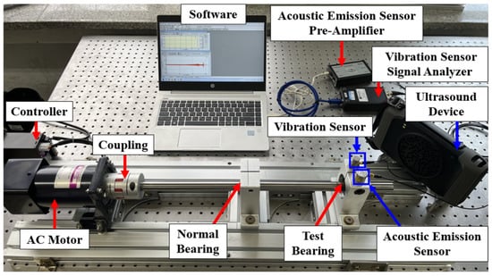
The experimental test rig was constructed on an anti-vibration table to minimize the influence of external disturbances, as illustrated in Figure 1. The table, supported by pneumatic isolation equipment, measures 1500 mm in length, 1000 mm in width, and 200 mm in height. Major components installed on the table include a controller, an AC motor, a coupling, a shaft, a bearing housing, and two ball bearings. The shaft used in the experiment has a diameter of 20 mm and a length of 55 mm. The first bearing is mounted 275 mm from the motor, and the distance between the two bearings is 160 mm. Specifications of the ball bearings are provided in Table 1; each bearing has a pitch diameter of 36 mm and contains seven rolling elements, each with a diameter of 9.52 mm.
Figure 1.
Experimental rig for ball bearing condition monitoring.
Table 1.
Specification of ball bearing.
Before testing, all bearings were thoroughly cleaned and uniformly re-lubricated with 4 g of NLGI Grade 2 grease to ensure consistency. The shaft was driven by a 180 W AC motor capable of operating at rotational speeds ranging from 90 to 1700 rpm. For the experiments reported in this study, the motor speed was fixed at 1500 rpm. A claw-type coupling (SJC-55C-RD, SUNG-IL Machinery Co., Ltd., Incheon, Republic of Korea) was used to connect the motor and shaft, allowing for slight angular and eccentric misalignments without compromising system stability.
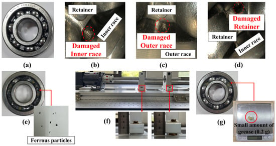
To comprehensively evaluate the diagnostic performance of the Ultra-based method, seven distinct bearing conditions were examined, as illustrated in Figure 2. These conditions include one normal state (N) and six fault conditions: inner race defect (I), outer race defect (O), retainer defect (R), contamination by ferrous particles (F), grease deficiency (G), and misalignment (M). Defects in the inner race, outer race, and retainer were artificially introduced using electric discharge machining (EDM) to ensure consistency in geometry and location. Misalignment was simulated by inserting washers beneath the bearing housing, creating a controlled vertical offset of 1 mm. Contamination by ferrous particles was replicated by incorporating a small quantity of ferrous debris into the lubricant, while grease deficiency was emulated by reducing the standard lubricant volume from 4 g to 0.2 g. Ferrous-particle contamination and grease starvation are common lubrication-related degradation modes in industrial applications and were therefore included to provide a more realistic assessment of diagnostic performance.
Figure 2.
Normal and defective conditions of ball bearings used in the experiment: (a) normal, (b) inner race defect, (c) outer race defect, (d) retainer defect, (e) contamination by ferrous particles, (f) misalignment, (g) grease deficiency.
For comparative performance evaluation across different condition monitoring approaches, three distinct sensors were employed simultaneously: a Vib (HS 13A231), an AE (PK3I), and an Ultra (BATCAM2, SM Instruments, Daejeon, Republic of Korea [28,65]). Ultrasonic measurement techniques generally fall into two categories: direct sensor attachment and remote sensing. In this study, the remote sensing approach was adopted to enable non-contact defect diagnosis, thereby mitigating issues related to sensor mounting, maintenance complexity, and long-term operational stability.
The sampling frequencies and corresponding frequency ranges for each sensor type are summarized in Table 2. The Vib operated at a sampling frequency of 12,000 Hz, capturing signals in the range of 0.5–10 kHz. The acoustic emission sensor collected data at 7168 Hz, covering a higher frequency range of 15–40 kHz. In contrast, the Ultra signals were captured at a frame rate of 30 frames per second (fps), effectively encompassing signal content within the 2–48 kHz frequency range.
Table 2.
Sampling frequency and frequency range of measurement sensors and equipment.
2.2. Data Acquisition
The sampling frequencies and measurement frequency ranges of the sensors are summarized in Table 2. The vibration (Vib) sensor acquired signals in the frequency range of 0.5–10,000 Hz at a sampling frequency of 12,000 Hz. The acoustic emission (AE) sensor collected high-frequency signals in the range of 15,000–40,000 Hz at a sampling frequency of 7168 Hz with a resonant frequency of 28,000 Hz. The ultrasonic visualization (Ultra) system operated at a frame rate of 30 fps and covered a frequency range of 2000–48,000 Hz.
To ensure a fair comparison, data from all sensors were acquired under identical operating conditions. As illustrated in Figure 3, the test rig was operated for an initial 20 min run-in period to minimize the influence of transient responses during system stabilization. Subsequently, data acquisition was performed five times at 10 min intervals. For each acquisition cycle, Vib and AE signals were recorded for 30 s, while the corresponding Ultra data were collected under the same operating conditions. This procedure yielded five measurement sets over a total monitoring period of 50 min.
Figure 3.
Data measurement methods using three types of sensors and devices (number of measurements and time).
To ensure consistency among sensing modalities, the Ultra data were synchronized with the corresponding Vib and AE measurements. The detailed measurement procedure is shown in Figure 3.
2.3. Proposed Method
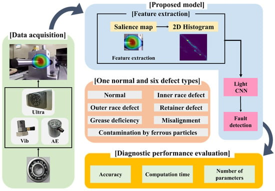
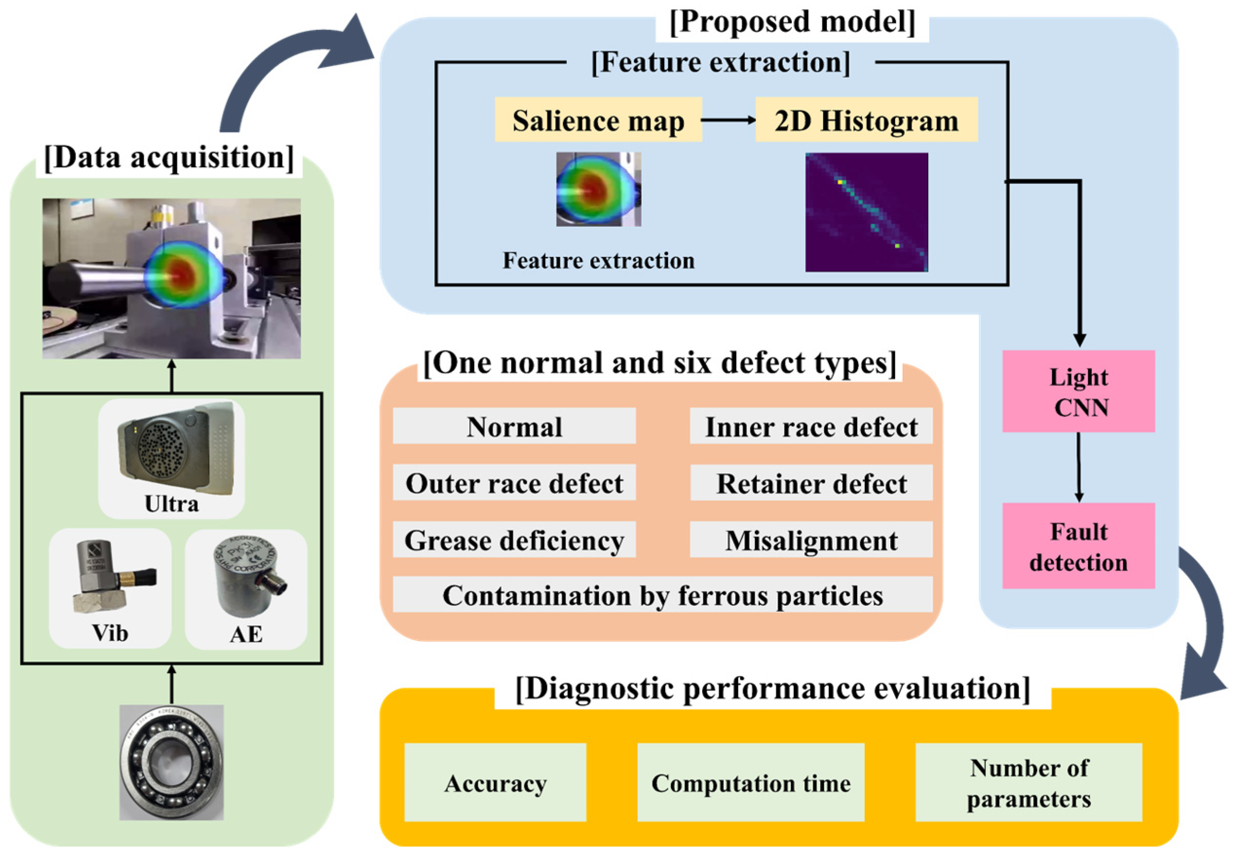
The entire workflow of the proposed ultra-based Light CNN model for diagnosing ball bearing conditions is depicted in Figure 4.
Figure 4.
A comprehensive methodology for diagnosing the condition of ball bearings.
The methodology begins with simultaneous data acquisition from three sensor types: vibration sensors (Vib), acoustic emission sensors (AE), and ultrasonic visualization equipment (Ultra). Measurements were conducted for one normal condition and six distinct defective conditions of ball bearings. Following data acquisition, preprocessing is performed to enhance data quality and reduce computational complexity, employing dimensionality reduction and feature extraction techniques, specifically saliency map generation and histogram-based transformations. Finally, fault diagnosis is performed by applying the preprocessed data to the proposed Light CNN model, with performance evaluated based on diagnostic accuracy, computational efficiency. Detailed explanations of the data preprocessing techniques and the structure of the proposed Light CNN are provided in Section 2.5 and Section 2.6, respectively.
2.4. Ultrasound Visualization Based on Beamforming
The beamforming refers to an array signal processing method that forms a beam from the phase information of waves propagating in space, using a distributed array of multiple sensors in space [70]. The beams are used to determine the location of a target of interest. For example, radar emits beams of electromagnetic waves to locate an aircraft. Since ultrasonic waves propagating through the air share similar properties with electromagnetic waves, it is possible to locate and track the source emitting ultrasonic waves by using an appropriate array of sensors capable of measuring them. Beamforming methods that visualize the location of a source by utilizing phase differences caused by spatial distribution differences in signals measured by each sensor are a kind of matched field processing technique. This approach involves modeling a basis function tailored to the characteristics of the source of interest, resulting in the highest beamforming power at the location where the signal most closely matches that basis function. Delay And Sum (DAS) is the oldest and the simplest array signal processing algorithm to form and steer beams.
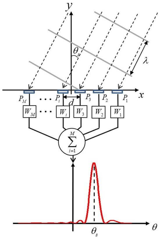
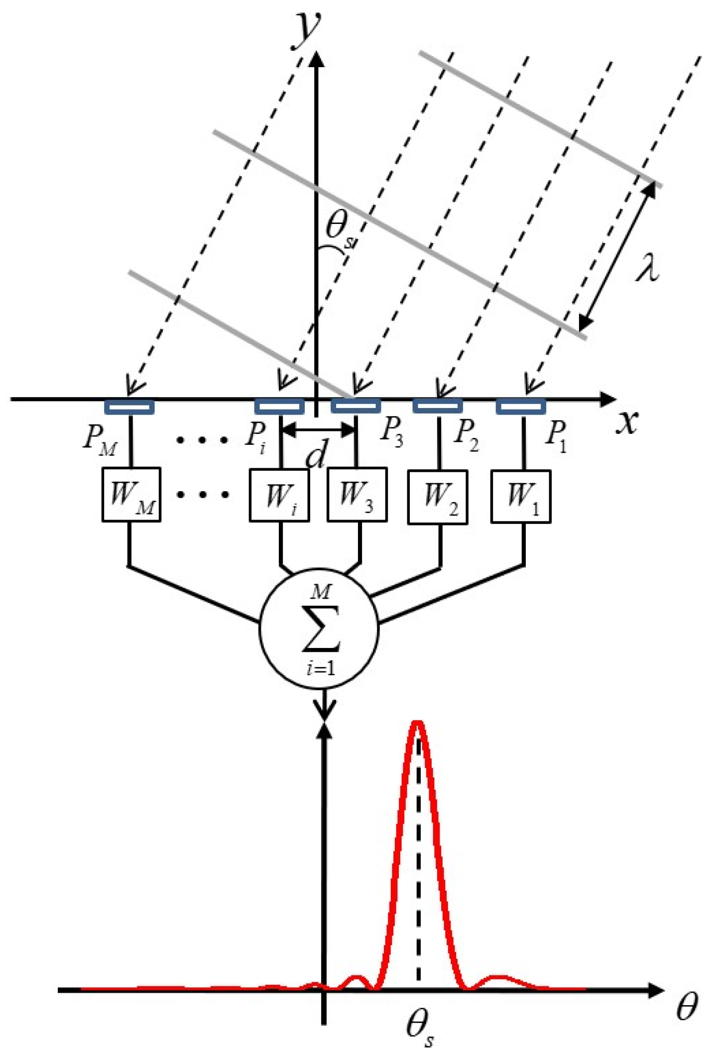
Figure 5 conceptually describes the DAS beamforming algorithm to estimate Direction of Arrival (DOA) with a 1-D linear array.
Figure 5.
A conceptual image of DAS beamforming.
For simplicity, a plane wave with a wavelength (λ) is incident into the array that has M sensors with an angle of θs. The incident waves are measured at each sensor element (Pi, i = 1, 2, 3, …, M). The signals contain time delays with respect to the position of the elements, and the signals are put into a series of scan vectors (Wi, i = 1, 2, 3, …, M) that have information on time delays corresponding to whole angle of interest. Then, the signals are calculated with the scan vectors by time shift in time domain or multiplication in frequency domain. (See Ref. [71] in detail).
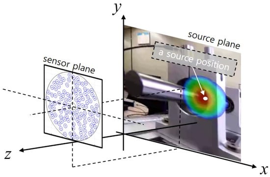
Based on the fundamentals above, the location of ultrasound source within the area of interest can be represented as a beam power distribution on a two-dimensional plane using the time delay information from each sensor element. By overlaying this image with an optical camera image, the location of the sound source can be intuitively visualized as shown in Figure 6. In this study, BATCAM2 from SMi Co., Ltd. (Daejeon, Republic of Korea), which has 112 sensor elements and the maximum frequency of 48 kHz, was used to acquire ultrasound fields. The array was designed as a sparse random array to measure shorter wavelength ultrasound than the size of sensor element, and the array configuration was optimized by genetic algorithm [72].
Figure 6.
Ultrasound visualization axes set-up and an example of ultrasound camera image (The size of the image is exaggerated compared to the ultrasound array).
2.5. Dimensionality Reduction Based on Key Information Features
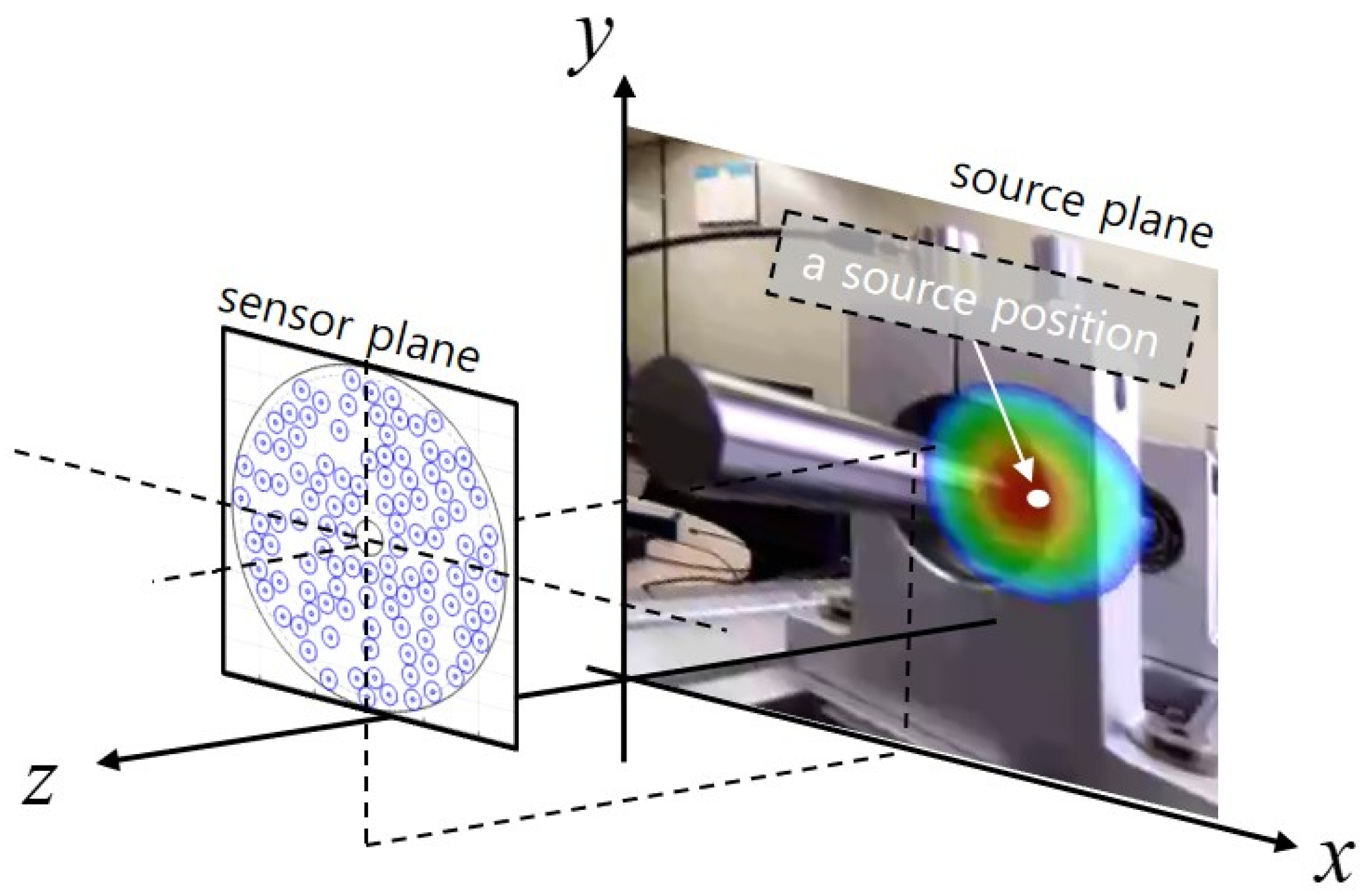
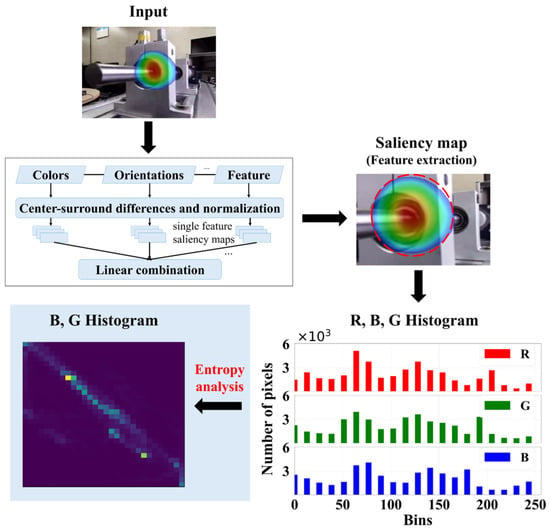
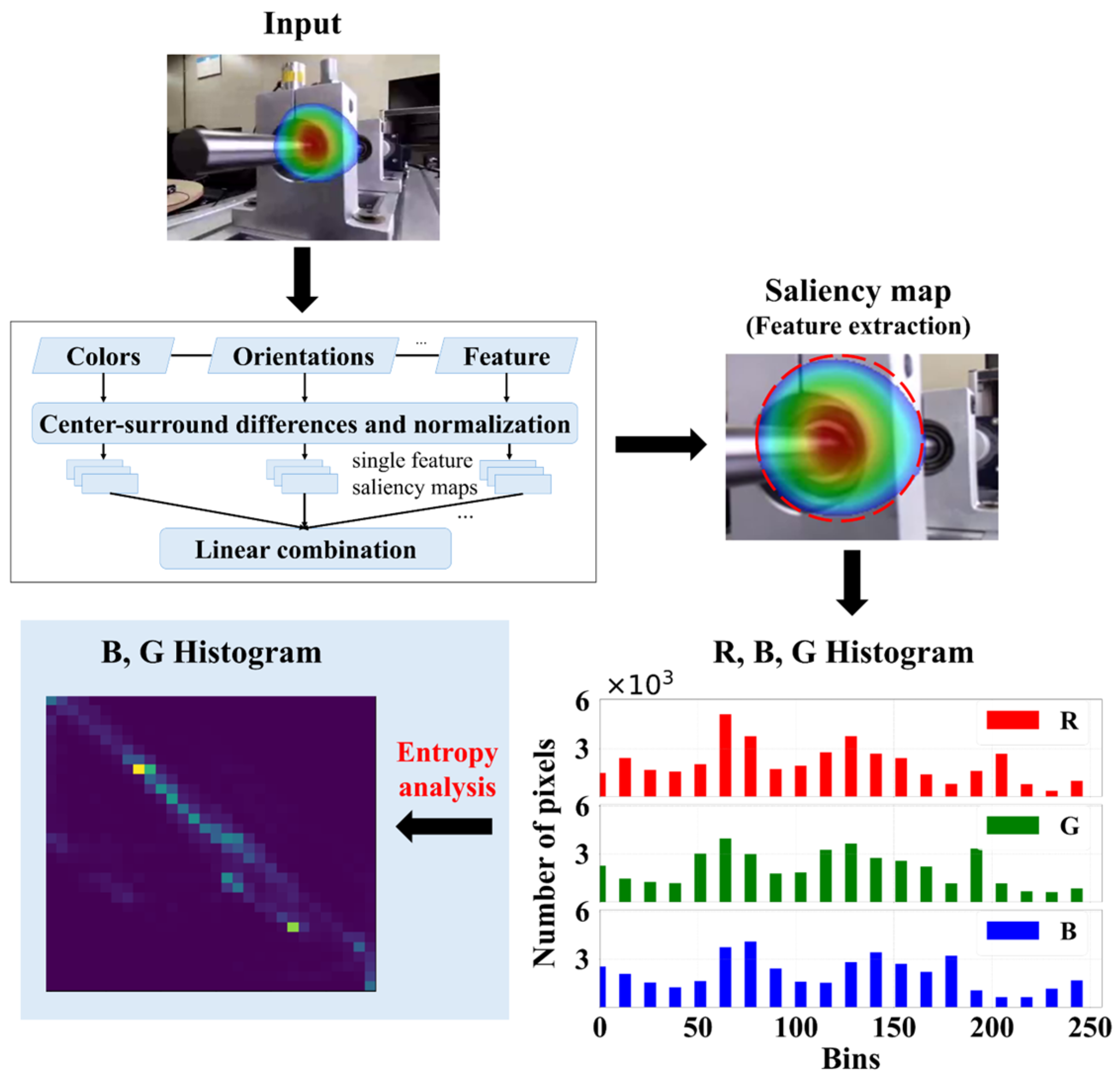
To enhance computational efficiency and facilitate effective feature extraction, the proposed Light CNN architecture is designed without pooling layers, which are conventionally used to reduce input dimensionality. Ultra signals, encoded as RGB images, contain critical defect-related information; however, they also include background elements that may obscure relevant fault features. To address this issue, saliency maps are used to isolate defect-specific regions from irrelevant background areas within the Ultra signals. The overall procedure for saliency map generation and the subsequent extraction of essential features is depicted in Figure 7.
Figure 7.
Process of generating saliency maps and extracting 2D histograms from RGB signals corresponding to defect regions.
As illustrated in Figure 7, the saliency map was generated through a three-step process. First, color, orientation, and feature information were extracted from the input image. Next, the center-surround difference method was applied to enhance the contrast between defect-related regions and the background, generating individual saliency maps for each feature. Finally, the individual saliency maps were combined using weighted linear fusion to produce the final saliency map, which was subsequently used to extract the defect-related region of interest (ROI).
To quantitatively assess the informational richness and relevance of the extracted color channels (R, G, and B), entropy analysis was conducted on the defect regions identified by the saliency map. Entropy serves as a statistical measure of randomness or uncertainty within the color data, indicating the potential informativeness of each channel. The average entropy values for the R, G, and B channels under various fault conditions are presented in Table 3, revealing that the B and G channels consistently exhibit higher entropy levels than the R channel. Based on this observation, the subsequent histogram-based feature extraction procedures primarily focused on the B and G channels to exploit their superior informational content.
Table 3.
Average entropy of RGB channels from Ultra signals under different bearing fault conditions.
Additionally, to effectively convert the extracted color information into compact numerical features, a two-dimensional histogram analysis was performed, with the optimal number of bins determined according to Sturges’ formula [73]. The pixel intensity range of the histogram was set to [0, 256], corresponding to the full range of an 8-bit image. The number of bins for the two-dimensional histogram was determined with reference to Sturges’ formula (). Considering the balance between computational efficiency and feature preservation, a histogram size of 20 × 20 was adopted. The resulting two-dimensional histogram combined the pixel intensity distributions of the G and B channels and consisted of a total of 400 features.
As a result, the extracted features were compressed into a compact 20 × 20 histogram representation, significantly reducing the computational burden and providing an efficient input structure for the subsequent Light CNN model.
2.6. Proposed Light Convolutional Neural Network Model
Convolutional Neural Networks (CNNs), inspired by biological visual perception mechanisms, exhibit strong generalization and learning capabilities. However, their computational complexity limits deployment in real-time and edge-computing environments. To address this issue, a lightweight CNN architecture (Light CNN) was developed using the essential fault-related features extracted from Ultra signals.
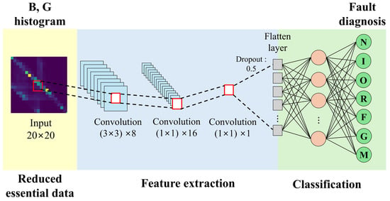
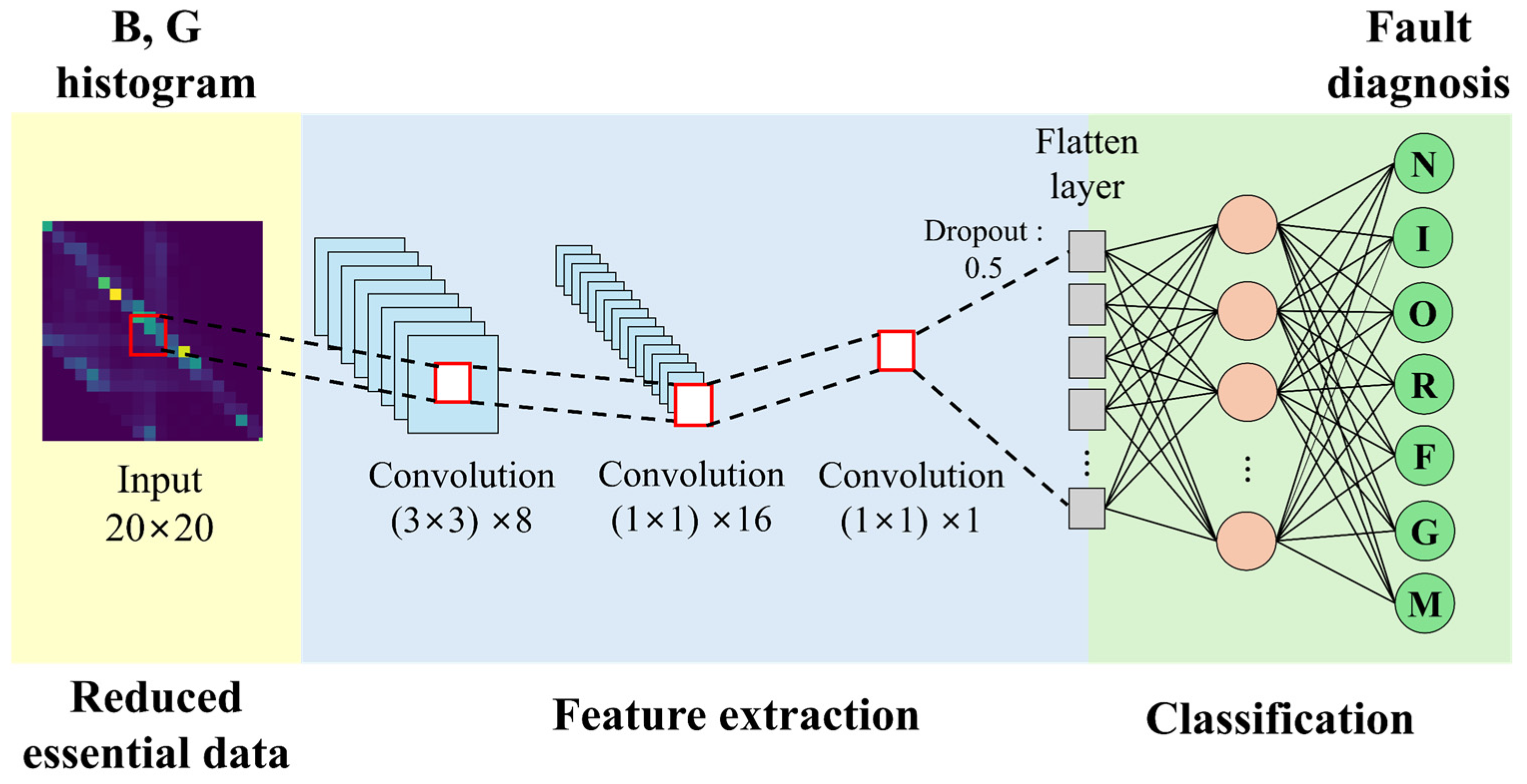
The proposed Light CNN uses a compact 20 × 20 BG histogram as input, preserving the essential fault-related information extracted during preprocessing. The network consists of an initial convolutional layer with eight 3 × 3 kernels, followed by two 1 × 1 convolutional layers with 16 and 1 kernels, respectively. Pooling layers were omitted because the input dimensionality had already been reduced during preprocessing.
Figure 8 illustrates the architecture of the proposed Light CNN. The first convolutional layer extracts local spatial features from the BG histogram, while the subsequent 1 × 1 convolutional layers reduce computational complexity while preserving discriminative fault-related information. A dropout rate of 0.5 is applied before the fully connected layer to improve generalization performance and reduce overfitting. Finally, a Softmax classifier is used to categorize the input into seven bearing conditions.
Figure 8.
Architecture of the proposed Light CNN model for bearing fault diagnosis.
The effectiveness of the proposed framework was evaluated through bearing fault classification experiments under various operating conditions. Diagnostic accuracy, computational efficiency, and robustness to speed variations were investigated to assess the practical applicability of the proposed method.
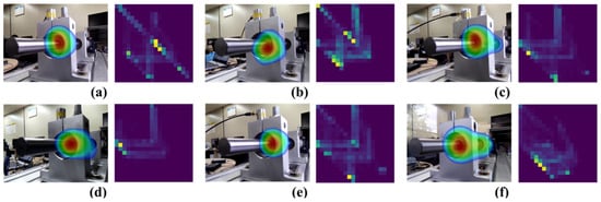
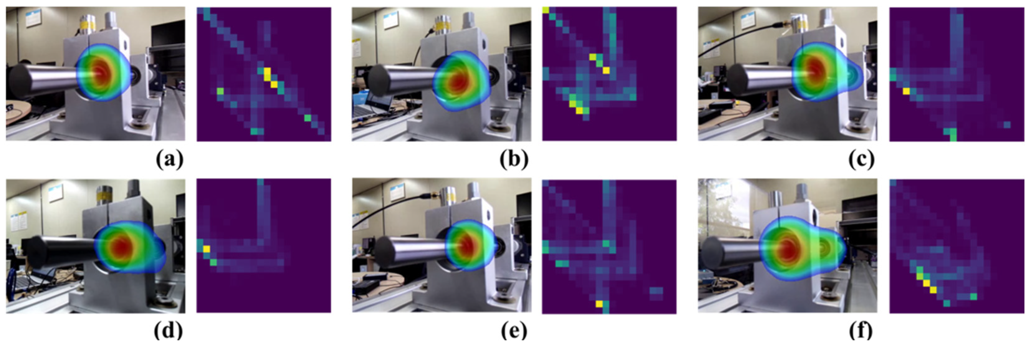
Figure 9 presents representative ultrasonic images and the corresponding BG color histograms for six bearing fault conditions, illustrating the distinct distribution patterns used as inputs to the proposed Light CNN.
Figure 9.
Color histogram analysis of Ultra signals for different ball bearing faults: (a) inner race defect, (b) outer race defect, (c) retainer defect, (d) contamination by ferrous particles, (e) misalignment, (f) grease deficiency.
3. Experimental Results and Discussion
3.1. Data Analysis
The collected dataset consisted of seven classes, including one healthy condition and six fault conditions, and comprised ultrasonic images, vibration signals, and acoustic emission (AE) signals. A total of 4200 samples were collected, with 600 samples for each class. To minimize the influence of class imbalance, an equal number of samples was as-signed to all classes, including ferrous-particle contamination and grease-starvation faults. For each experimental run, the dataset was randomly divided into 300 training samples, 100 validation samples, and 200 test samples per class. The entire procedure, including data splitting, preprocessing, model training, and evaluation, was independently repeated ten times. The final results were reported as the average performance across the ten runs.
All experiments were conducted on a workstation equipped with an Intel Core i9-10900F CPU, 128 GB RAM, and an NVIDIA GeForce RTX 4090 GPU with 24 GB memory.
To analyze the characteristics of the acquired signals and evaluate the separability of different fault conditions, spectrogram and principal component analyses were performed for the three sensing modalities.
The parameters used for spectrogram generation are summarized in Table 4. Vib and AE signals were transformed into time–frequency representations using the Short-Time Fourier Transform (STFT), and the resulting spectrograms were used for subsequent analysis.
Table 4.
Parameters and time intervals for generating spectrograms for two sensors Vib and AE.
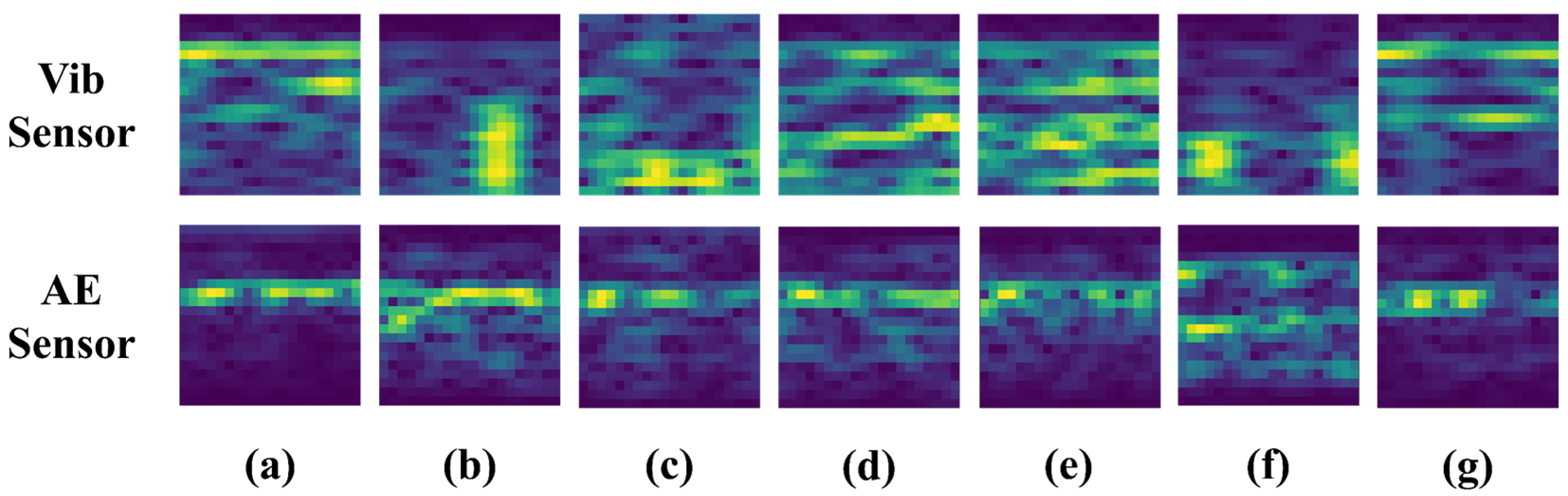
Representative spectrograms of different bearing conditions are presented in Figure 10. The Vib and AE signals exhibited distinct time–frequency characteristics under different fault conditions. However, several fault classes showed similar spectral patterns, making visual discrimination difficult in some cases.
Figure 10.
Spectrogram examples of ball bearing conditions based on Vib and AE signals: (a) normal, (b) inner race defect, (c) outer race defect, (d) retainer defect, (e) contamination by ferrous particles, (f) misalignment, (g) grease deficiency.
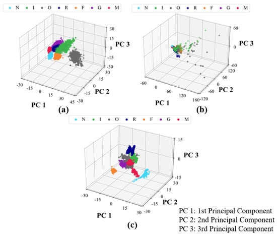
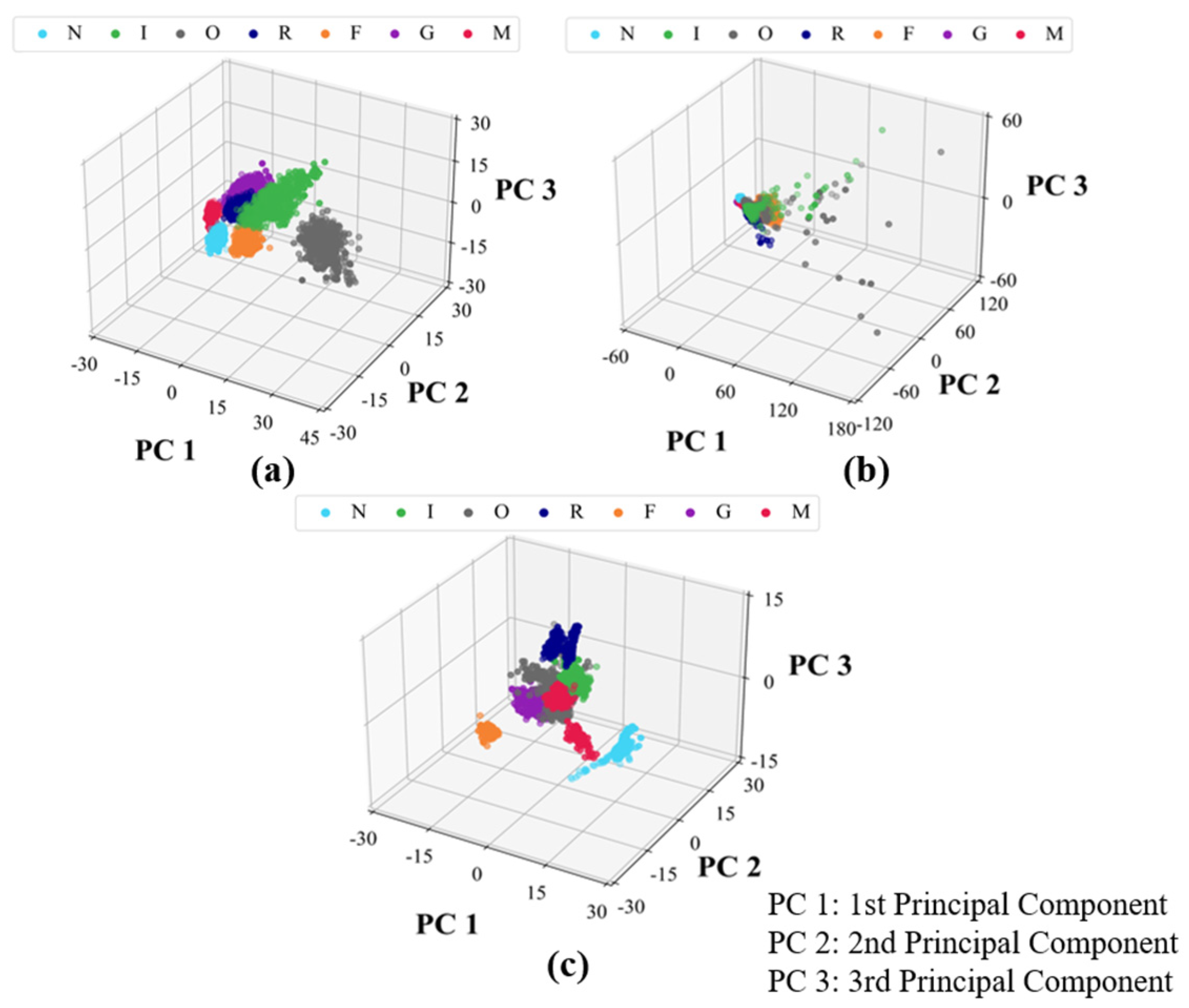
To further evaluate class separability, Principal Component Analysis (PCA) was applied to the Ultra, Vib, and AE datasets. The PCA results are shown in Figure 11. Compared with the Vib and AE datasets, the Ultra data formed more compact and clearly separated clusters for individual fault classes. In contrast, partial overlap between fault classes was observed in the Vib and AE datasets. These results indicate that the ultrasonic visualization data provide better class separability than Vib and AE signals, which is consistent with the superior classification performance achieved by the proposed framework.
Figure 11.
PCA of three-sensor bearing fault signals: (a) Vib signals, (b) AE signals, (c) Ultra signals.
3.2. Performance Comparison of Fault Diagnosis Using Signals from Three Different Sensors
To compare the diagnostic performance of different sensing modalities, the proposed Light CNN was applied to the Ultra, AE, and Vib datasets. For a fair comparison, all experiments were conducted using the same network architecture and training settings, including the Adam optimizer, a batch size of 32, and 100 epochs. Classification performance was evaluated using Accuracy, F1-score, Precision, and Recall. The minimum, maximum, mean, and standard deviation values from ten independent runs are summarized in Table 5.
Table 5.
Classification performance of Ultra, AE, and Vib sensors under the 1500 rpm operating condition.
As shown in Table 5, the Ultra sensor achieved the highest average accuracy of 99.98%, outperforming the AE (98.64%) and Vib (99.46%) sensors. It also exhibited the lowest standard deviation (0.00026), indicating superior stability across repeated experiments. Similar trends were observed for F1-score, Precision, and Recall, with the Ultra sensor consistently achieving the best performance among the three sensing modalities.
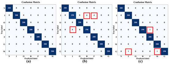
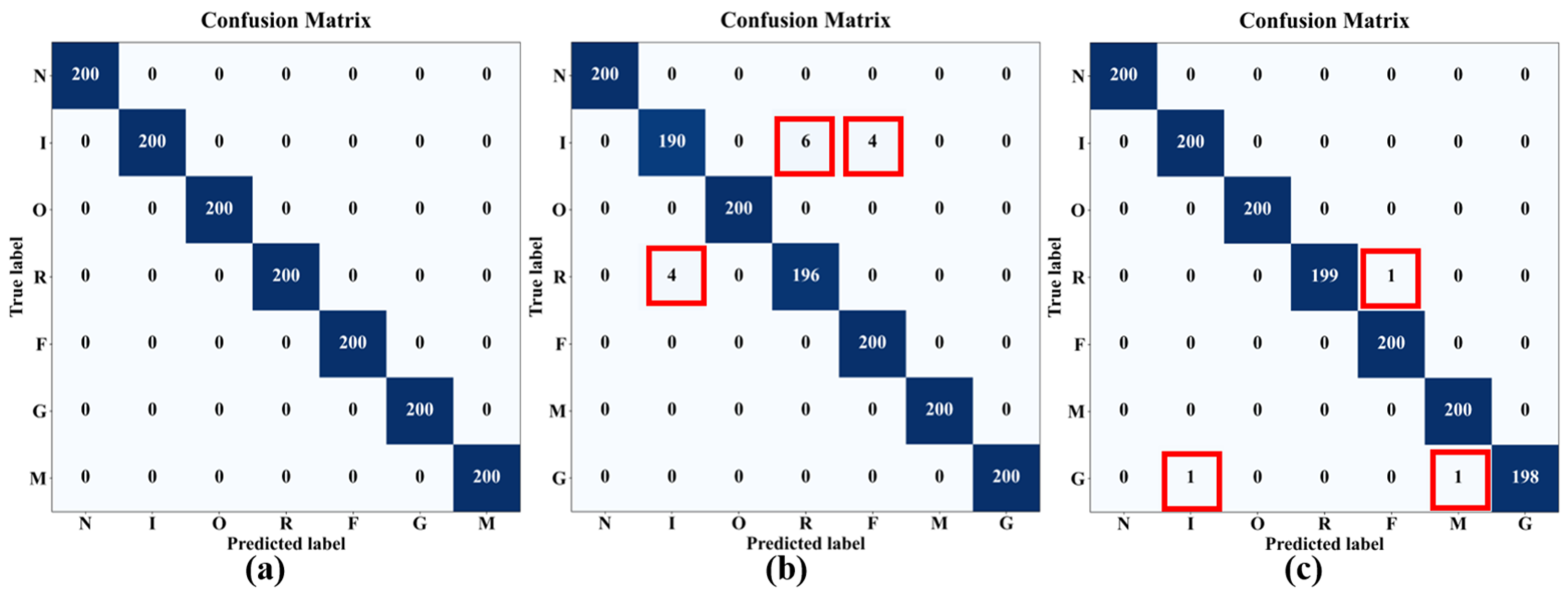
Representative confusion matrices for the three sensing modalities are shown in Figure 12. The Ultra sensor achieved perfect classification across all seven classes, with no misclassified samples observed. In contrast, the AE sensor exhibited misclassifications among the inner-race defect (I), retainer defect (R), ferrous-particle contamination (F), and normal (N) classes. The Vib sensor showed only three misclassified samples involving the retainer defect (R), grease-starvation (G), and misalignment (M) classes. Consistent with the results in Table 5, the Ultra sensor demonstrated the highest classification accuracy, followed by the Vib and AE sensors.
Figure 12.
Comparison of confusion matrices for fault diagnosis using (a) Ultra, (b) AE, and (c) Vib sensors at 1500 rpm.
To evaluate computational efficiency, the preprocessing time and inference through-put (IPS) were compared, as summarized in Table 6. The Ultra sensor achieved an average preprocessing time of 0.00099 s and an average throughput of 11.47 IPS, whereas the AE and Vib sensors achieved 1.11 IPS and 1.22 IPS, respectively. Although the preprocessing times were similar across all sensing modalities, the Ultra-based framework provided approximately nine times higher inference through-put than the AE- and Vib-based approaches. These results indicate that the proposed framework achieves both superior diagnostic performance and high computational efficiency, demonstrating its potential for real-time bearing fault diagnosis applications.
Table 6.
Performance comparison of Ultra, AE and Vib signals using time.
The results in Table 6 demonstrate that the proposed Ultra-based framework achieves both high classification performance and computational efficiency. The high inference throughput further indicates its suitability for real-time condition monitoring and edge deployment.
3.3. Comparison of the Proposed Light CNN with Existing Lightweight Models
To evaluate the diagnostic performance and computational efficiency of the proposed model, comparative experiments were conducted using three representative lightweight CNN architectures: MobileNet [56], ShuffleNet [57], and EfficientNet-eLite [58]. Since these models were originally designed for 224 × 224 RGB image inputs, minor architectural modifications were made to accommodate the 20 × 20 histogram inputs used in this study. Specifically, stride = 2 operations were removed to prevent excessive feature-map reduction, and the 7 × 7 average pooling layer was replaced with a 5 × 5 layer. In addition, EfficientNet-eLite and ShuffleNet were scaled using d4 = 0.5 and 0.25× (g = 2), respectively. All models were trained using the same dataset and Adam optimizer settings to ensure a fair comparison. Model size was calculated assuming FP32 storage (4 bytes per parameter). The comparison was performed using the Ultra dataset collected at 1500 rpm, and the results are summarized in Table 7.
Table 7.
Performance comparison of the proposed model with MobileNet, ShuffleNet, and EfficientNet-eLite.
As shown in Table 7, the proposed model achieved the highest classification accuracy of 99.99%, exceeding EfficientNet-eLite (98.99%), MobileNet (99.79%), and ShuffleNet (99.78%). The proposed model also exhibited the shortest inference time (0.134 s), com-pared with 0.718 s, 0.229 s, and 1.507 s for EfficientNet-eLite, MobileNet, and ShuffleNet, respectively. These results demonstrate that the proposed architecture provides an effective balance between diagnostic accuracy and computational efficiency for compact histogram-based feature representations.
To further evaluate the classification performance, the Area Under the Receiver Operating Characteristic Curve (AUC) was calculated. AUC quantifies the overall ability of a classifier to distinguish between classes, with values closer to 1 indicating better discriminative performance. In addition, p-values were computed to assess whether the performance differences between the proposed model and the benchmark models were statistically significant. A p-value below 0.05 was considered indicative of a statistically significant difference. The corresponding results are summarized in Table 8.
Table 8.
Comparison of AUC performance and statistical significance between the proposed model and lightweight architectures.
As shown in Table 8, the proposed model achieved a Micro-AUC of 100% and a Macro-AUC of 99.49%, indicating excellent discriminative capability across all fault classes. Furthermore, all p-values were below 0.05, confirming that the performance differences between the proposed model and the benchmark models were statistically significant.
The AUC and p-value results were consistent with the accuracy-based evaluation. The proposed model achieved competitive discriminative performance while maintaining statistical significance against the benchmark models. Combined with its low computational cost, these results demonstrate the effectiveness of the proposed architecture for lightweight fault diagnosis applications.
3.4. Performance Evaluation Under Different Operating Speeds (500 rpm)
To evaluate the robustness of the proposed framework under different operating conditions, additional experiments were conducted at 500 rpm using the same procedure and evaluation protocol as those used under the rated-speed condition (1500 rpm). Since operating speed affects the characteristics of vibration, acoustic emission, and ultrasonic signals generated by bearing defects, performance evaluation under low-speed conditions is important for assessing the practical applicability of a fault diagnosis system.
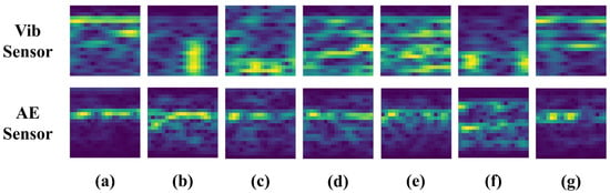
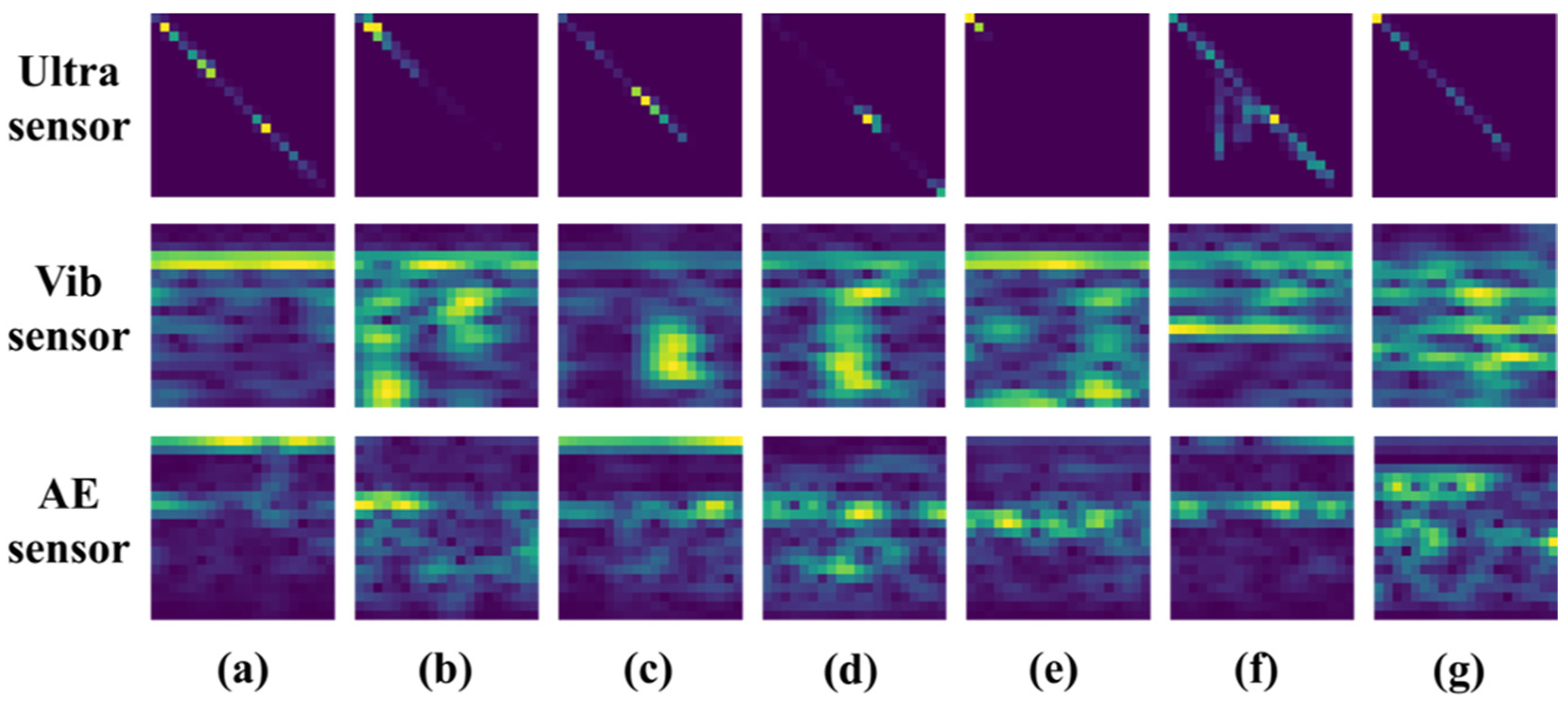
Figure 13 presents representative feature representations obtained from the Ultra, Vib, and AE signals under the 500 rpm condition. Distinct feature patterns corresponding to different fault conditions can be observed in all three sensing modalities. However, the Ultra data exhibited clearer pattern variations among fault classes, whereas several fault conditions showed relatively similar feature distributions in the Vib and AE data. These observations suggest that fault-related information remained visually distinguishable in the Ultra data even under low-speed operation.
Figure 13.
Spectrogram examples of ball bearing conditions at 500 rpm, obtained using Ultra, Vib, and AE signals: (a) normal, (b) inner race defect, (c) outer race defect, (d) retainer defect, (e) contamination by ferrous particles, (f) misalignment, (g) grease deficiency.
The quantitative classification results are summarized in Table 9. The Ultra sensor achieved an average accuracy of 99.96%, representing only a 0.02 percentage-point decrease compared with the 1500 rpm condition (99.98%). The AE sensor achieved an average accuracy of 99.74%, which was higher than that obtained under the rated-speed condition (98.64%). In contrast, the Vib sensor achieved an average accuracy of 97.01%, corresponding to a decrease of 2.45 percentage points from the 1500 rpm condition (99.46%). The minimum accuracy of the Vib sensor also decreased to 96.64%, whereas the Ultra and AE sensors maintained minimum accuracies above 99%.
Table 9.
Classification performance of Ultra, AE, and Vib sensors at 500 rpm.
Overall, the Ultra sensor achieved the highest classification performance under both rated-speed and low-speed operating conditions, demonstrating stable diagnostic capability across different operating speeds.
3.5. Discussion
The experimental results demonstrated that the proposed Ultra-based Light CNN framework outperformed vibration- and acoustic-emission-based approaches. This performance difference can be attributed to the fundamental sensing principles of the three modalities.
Vibration-based methods rely on indirect measurements, where defect-induced signals propagate through the shaft, bearing housing, and surrounding mechanical structures before reaching the sensor. Consequently, the measured signals may be affected by attenuation, structural resonances, and environmental noise, making fault characteristics less distinguishable under varying operating conditions. Consistent with this observation, the Vib sensor exhibited reduced classification performance under the 500 rpm condition.
AE techniques detect high-frequency elastic waves generated by friction, crack propagation, and localized impacts, making them highly sensitive to incipient defects. However, measurement quality can be influenced by sensor mounting and coupling conditions, and defect-location information is not directly available.
In contrast, the ultrasonic visualization approach employs a beamforming-based technique that spatially localizes ultrasonic energy radiated from defect regions. As a result, the influence of structural transmission paths is reduced, allowing defect characteristics to be captured more directly. These properties likely contributed to the consistently high classification performance achieved under both 1500 rpm and 500 rpm operating conditions.
The proposed Saliency Map-based ROI extraction and BG histogram representation reduced the input size to 20 × 20 pixels while preserving discriminative information, enabling both high diagnostic accuracy and computational efficiency.
Compared with previous lightweight deep-learning studies [54,55,56,57,58,59,60], the proposed framework differs in several aspects. Most existing lightweight CNN approaches have focused on vibration or AE signals, whereas this study utilizes ultrasonic visualization data. Furthermore, compact feature maps are generated through Saliency Map-based ROI extraction and BG histogram representation before classification, enabling the use of a simple three-layer Light CNN. In addition, vibration, AE, and ultrasonic sensing modalities were directly compared under identical experimental conditions, including ferrous-particle contamination and grease-starvation faults. These characteristics distinguish the proposed framework from previous lightweight CNN-based bearing fault diagnosis studies.
The average inference throughput of 11.47 IPS further demonstrates the feasibility of combining ultrasonic visualization with lightweight deep learning for real-time condition monitoring and edge-computing applications.
Several limitations should be acknowledged. The experiments were conducted on a laboratory-scale test rig under controlled operating conditions, and only single-fault scenarios were considered. Therefore, additional validation under compound-fault, varying-load, and noisy operating conditions is required.
Despite these limitations, the proposed approach shows potential for industrial condition-monitoring applications. Its non-contact sensing capability reduces issues associated with sensor mounting and coupling, while the lightweight architecture provides computational efficiency suitable for real-time implementation. Future work will focus on validating the framework using data acquired from industrial equipment operating under diverse environmental and operational conditions.
4. Conclusions
This study proposed a non-contact ball bearing fault diagnosis framework that combines RGB data acquired from an ultrasonic visualization system with a lightweight convolutional neural network (Light CNN). The proposed method employed Saliency Map- and BG Histogram-based feature extraction to generate compact input representations, which were subsequently classified using a lightweight CNN architecture. Diagnostic performance was evaluated for seven bearing conditions, including a healthy state, inner-race defect, outer-race defect, retainer defect, ferrous-particle contamination, grease starvation, and misalignment. In addition, vibration, acoustic emission (AE), and ultra-sonic sensing modalities were compared under identical experimental conditions.
Experimental results showed that the proposed method achieved an average classification accuracy and F1-score of 99.98%, outperforming both vibration- and AE-based approaches. The proposed framework also demonstrated high computational efficiency, achieving an average inference throughput of 11.47 IPS while maintaining stable diagnostic performance under the low-speed operating condition of 500 rpm. Furthermore, high classification performance was achieved for ferrous-particle contamination and grease-starvation faults, which have received relatively limited attention in previous studies.
These results demonstrate the effectiveness of ultrasonic visualization for non-contact bearing fault diagnosis and indicate that the combination of compact feature reprsentations and a lightweight CNN can provide both high diagnostic accuracy and computational efficiency. Future work will focus on validating the proposed framework using industrial machinery operating under diverse environmental and loading conditions to further assess its generalization capability and practical applicability.
Author Contributions
Conceptualization, S.-H.H. and C.-S.P.; methodology, H.J.; software, H.J.; validation, H.J., M.K. and M.D.; formal analysis, H.J.; investigation, H.J.; resources, H.J.; data curation, M.K. and M.D.; writing—original draft preparation, H.J. and S.-H.H.; writing—review and editing, S.-H.H. and S.-W.B.; visualization, H.J.; supervision, S.-W.B.; project administration, S.-H.H.; funding acquisition, S.-W.B. and S.-H.H. All authors have read and agreed to the published version of the manuscript.
Funding
This research received no external funding.
Data Availability Statement
All relevant data are provided within the manuscript.
Acknowledgments
This work was supported by the 2026 Yeungnam University Research Grant.
Conflicts of Interest
The authors declare no conflicts of interest.
Abbreviations
| CNN | Convolutional Neural Networks |
| RMS | Root Mean Square |
| FFT | Fast Fourier Transform |
| STFT | Short-Time Fourier Transform |
| SP | Signal Processing |
| ML | Machine Learning |
| DL | Deep Learning |
| SVM | Support Vector Machines |
| RF | Random Forests |
| KNN | K-Nearest Neighbors |
| EDM | Electric Discharge Machining |
| Vib | Vibration |
| AE | Acoustic Emission |
| Ultra | Ultrasonic |
| DAS | Delay And Sum |
| DOA | Direction of Arrival |
| IPS | Inferences Per Second |
| PCA | Principal Component Analysis |
| SCADA | Supervisory Control and Data Acquisition |
References
- Karnavas, Y.L.; Plakias, S.; Chasiotis, I.D. Extracting spatially global and local attentive features for rolling bearing fault diagnosis in electrical machines using attention stream networks. IET Electr. Power Appl. 2021, 15, 903–915. [Google Scholar] [CrossRef] [Scilit]
- Qin, Y.; Jin, L.; Zhang, A.; He, B. Rolling bearing fault diagnosis with adaptive harmonic kurtosis and improved bat algorithm. IEEE Trans. Instrum. Meas. 2021, 70, 3508112. [Google Scholar] [CrossRef] [Scilit]
- Randall, R.B.; Antoni, J. Rolling element bearing diagnostics—A tutorial. Mech. Syst. Signal Process. 2011, 25, 485–520. [Google Scholar] [CrossRef] [Scilit]
- Wang, D.; Zhao, Y.; Yi, C.; Tsui, K.L.; Lin, J. Sparsity guided empirical wavelet transform for fault diagnosis of rolling element bearings. Mech. Syst. Signal Process. 2018, 101, 292–308. [Google Scholar] [CrossRef] [Scilit]
- Tomovic, R.; Miltenovic, V.; Banic, M.; Miltenovic, A. Vibration response of rigid in unloaded rolling element bearing. Int. J. Mech. Sci. 2010, 52, 1176–1185. [Google Scholar] [CrossRef] [Scilit]
- Mohd, Y.N.F.; Ripin, Z.M. Analysis of surface parameters and vibration of rolling bearing. Tribol. Trans. 2014, 57, 715–729. [Google Scholar] [CrossRef] [Scilit]
- Hoeprich, M.R. Rolling element bearing fatigue damage propagation. J. Tribol. 1992, 114, 328–333. [Google Scholar] [CrossRef] [Scilit]
- Brie, D. Modelling of the spalled rolling element bearing vibration signal: An overview and some new results. Mech. Syst. Signal Process. 2000, 14, 353–369. [Google Scholar] [CrossRef] [Scilit]
- Singh, S.; Kumar, N. Detection of bearing faults in mechanical system using stator current monitoring. IEEE Trans. Ind. Inform. 2017, 13, 1341–1349. [Google Scholar] [CrossRef] [Scilit]
- Patel, V.N.; Tandon, N.; Pandey, R.K. Vibrations generated by rolling element bearings having multiple local defects on races. Procedia Technol. 2014, 14, 312–319. [Google Scholar] [CrossRef] [Scilit]
- Mogal, S.P.; Bhandare, R.V.; Phalle, V.M.; Kushare, P.B. Fault diagnosis and prediction of remaining useful life (RUL) of rolling element bearing: A review state of art. Tribologia 2024, 41, 28–42. [Google Scholar] [CrossRef] [Scilit]
- Gao, S.; Han, Q.; Pennacchi, P.; Chatterton, S.; Chu, F. Dynamic, thermal, and vibrational analysis of ball bearings with over-skidding behavior. Friction 2023, 11, 580–601. [Google Scholar] [CrossRef] [Scilit]
- Yu, X.; Liang, Z.; Wang, Y.; Yin, H.; Liu, X.; Yu, W.; Huang, Y. A wavelet packet transform-based deep feature transfer learning method for bearing fault diagnosis under different working conditions. Measurement 2022, 201, 111597. [Google Scholar] [CrossRef] [Scilit]
- Xu, M.; Miao, D.; Gao, Y.; Yang, R.; Gu, F.; Shao, Y. A bearing dynamic model based on novel Gaussian-filter waviness characterizing method for vibration response analysis. Tribol. Int. 2024, 194, 109433. [Google Scholar] [CrossRef] [Scilit]
- Ma, Z.; Zhao, M.; Luo, M.; Gou, C.; Xu, G. An integrated monitoring scheme for wind turbine main bearing using acoustic emission. Signal Process. 2023, 205, 108867. [Google Scholar] [CrossRef] [Scilit]
- Huang, S.; Li, J.; Wu, L.; Zhang, W. Research on acoustic fault diagnosis of bearings based on spatial filtering and time-frequency domain filtering. Measurement 2023, 221, 113533. [Google Scholar] [CrossRef] [Scilit]
- Liu, Z.; Li, H.; Jiao, J.; Shen, T.; Zhang, B.; Liu, H. A novel acoustic emission signal segmentation network for bearing fault fingerprint feature extraction under varying speed conditions. Eng. Appl. Artif. Intell. 2023, 126, 106819. [Google Scholar] [CrossRef] [Scilit]
- Kim, S.J.; Kim, K.; Hwang, T.; Park, J.; Jeong, H.; Kim, T.; Youn, B.D. Motor-current-based electromagnetic interference de-noising method for rolling element bearing diagnosis using acoustic emission sensors. Measurement 2022, 193, 110912. [Google Scholar] [CrossRef] [Scilit]
- He, F.; Xie, G.; Luo, J. Electrical bearing failures in electric vehicles. Friction 2020, 8, 4–28. [Google Scholar] [CrossRef] [Scilit]
- Martine, G.; Becker, F.M.; Kirchner, E. A novel method for diagnosing rolling bearing surface damage by electric impedance analysis. Tribol. Int. 2022, 170, 107503. [Google Scholar] [CrossRef] [Scilit]
- Feng, S.; Zhang, J.; Fan, B.; Su, Z.; Lu, S. A panoramic ferrograph for on-site detection of oil wear debris. Tribol. Int. 2023, 190, 109025. [Google Scholar] [CrossRef] [Scilit]
- Lin, C.L.; Meehan, P.A. Morphological and elemental analysis of wear debris naturally formed in grease lubricated railway axle bearings. Wear 2021, 484–485, 203994. [Google Scholar] [CrossRef] [Scilit]
- Atif, M.; Azmat, S.; Khan, F.; Albogamy, F.R.; Khan, A. AI-driven thermography-based fault diagnosis in single-phase induction motor. Results Eng. 2024, 24, 103493. [Google Scholar] [CrossRef] [Scilit]
- Roldan, S.; Sanchez-Londono, D.; Barbieri, G. Thermographic indicator for the state assessment of rolling bearings. IFAC-PapersOnLine 2021, 54, 1218–1223. [Google Scholar] [CrossRef] [Scilit]
- Choudhary, A.; Mian, T.; Fatima, S. Convolutional neural network based bearing fault diagnosis of rotating machine using thermal images. Measurement 2021, 176, 109196. [Google Scholar] [CrossRef] [Scilit]
- Niu, S.; Srivastava, V. Simulation trained CNN for accurate embedded crack length, location, and orientation prediction from ultrasound measurements. Int. J. Solids Struct. 2022, 242, 111521. [Google Scholar] [CrossRef] [Scilit]
- Verellen, T.; Verbelen, F.; Stockman, K.; Steckel, J. Beamforming applied to ultrasound analysis in detection of bearing defects. Sensors 2021, 21, 6803. [Google Scholar] [CrossRef] [Scilit] [PubMed]
- Lee, J.H.; Kim, Y.S.; Rehman, A.; Kim, I.K.; Lee, J.J.; Yun, H.S. Development of an AI-based image/ultrasonic convergence camera system for accurate gas leak detection in petrochemical plants. Heliyon 2024, 10, e28905. [Google Scholar] [CrossRef] [Scilit] [PubMed]
- Koene, I.; Haikonen, S.; Tiainen, T.; Keski-Rahkonen, J.; Manngård, M.; Viitala, R. On-shaft wireless vibration measurement unit and signal processing method for torsional and lateral vibration. IEEE/ASME Trans. Mechatron. 2022, 27, 5857–5868. [Google Scholar] [CrossRef] [Scilit]
- Petersen, D.; Howard, C.; Sawalhi, N.; Ahmadi, A.M.; Singh, S. Analysis of bearing stiffness variations, contact forces and vibrations in radially loaded double row rolling element bearings with raceway defects. Mech. Syst. Signal Process. 2015, 50, 139–160. [Google Scholar] [CrossRef] [Scilit]
- Sghir, K.A.; Bolaers, F.; Cousinard, O.; Dron, J.P. Vibratory monitoring of a spalling bearing defect in variable speed regime. Mech. Ind. 2013, 14, 129–136. [Google Scholar] [CrossRef] [Scilit]
- Nikolaou, N.G.; Antoniadis, I.A. Rolling element bearing fault diagnosis using wavelet packets. NDT E Int. 2002, 35, 197–205. [Google Scholar] [CrossRef] [Scilit]
- Ho, D.; Randall, R.B. Optimisation of bearing diagnostic techniques using simulated and actual bearing fault signal. Mech. Syst. Signal Process. 2000, 14, 763–788. [Google Scholar] [CrossRef] [Scilit]
- Mbo’o, C.P.; Hameyer, K. Fault diagnosis of bearing damage by means of the linear discriminant analysis of stator current features from the frequency selection. IEEE Trans. Ind. Appl. 2016, 52, 3861–3868. [Google Scholar] [CrossRef] [Scilit]
- Abu-Zeid, M.A.; Abdel-Rahman, S.M. Bearing problems’ effects on dynamic performance of pumping stations. Alex. Eng. J. 2013, 52, 241–248. [Google Scholar] [CrossRef] [Scilit]
- Tabasi, M.; Ojaghi, M.; Mostafavi, M. Vibration analysis as useful domain for detection of bearing fault signals in induction motors. Int. J. Eng. Trans. B Appl. 2021, 34, 2010–2020. [Google Scholar] [CrossRef] [Scilit]
- Qiu, H.; Lee, J.; Lin, J.; Yu, G. Wavelet filter-based weak signature detection method and its application on rolling element bearing prognostics. J. Sound Vib. 2006, 289, 1066–1090. [Google Scholar] [CrossRef] [Scilit]
- Wang, C.; Gao, R.X. Wavelet transform with spectral post-processing for enhanced feature extraction. IEEE Trans. Instrum. Meas. 2003, 52, 1296–1301. [Google Scholar] [CrossRef]
- Cheng, J.; Yu, D.; Yu, Y. Application of an impulse response wavelet to fault diagnosis of rolling bearings. Mech. Syst. Signal Process. 2007, 21, 920–929. [Google Scholar] [CrossRef] [Scilit]
- Muhashi, A.; Feng, X.; Onishi, Y.; Ota, R.; Liu, H. Enhancing Coincidence Time Resolution of PET detectors using short-time Fourier transform and residual neural network. Nucl. Instrum. Methods Phys. Res. Sect. A 2024, 1065, 169540. [Google Scholar] [CrossRef] [Scilit]
- Patel, R.K.; Giri, V.K. Condition monitoring of induction motor bearing based on bearing damage index. Arch. Electr. Eng. 2017, 66, 105–119. [Google Scholar] [CrossRef] [Scilit]
- Xie, Z.; Chen, J.; Shi, Z.; Liu, S.; He, S. Lightweight pyramid attention residual network for intelligent fault diagnosis of machine under sharp speed variation. Mech. Syst. Signal Process. 2025, 223, 111824. [Google Scholar] [CrossRef] [Scilit]
- Hakim, M.; Omran, A.A.B.; Ahmed, A.N.; Al-Waily, M.; Abdellatif, A. A systematic review of rolling bearing fault diagnoses based on deep learning and transfer learning: Taxonomy, overview, application, open challenges, weaknesses and recommendations. Ain Shams Eng. J. 2023, 14, 101945. [Google Scholar] [CrossRef] [Scilit]
- Wang, X.; Shen, C.; Xia, M.; Wang, D.; Zhu, J.; Zhu, Z. Multi-scale deep intra-class transfer learning for bearing fault diagnosis. Reliab. Eng. Syst. Saf. 2020, 202, 107050. [Google Scholar] [CrossRef] [Scilit]
- Hu, Q.; Si, X.S.; Zhang, Q.H.; Qin, A.S. A rotating machinery fault diagnosis method based on multi-scale dimensionless indicators and random forests. Mech. Syst. Signal Process. 2020, 139, 106609. [Google Scholar] [CrossRef] [Scilit]
- Zhang, W.; Li, X.; Ding, Q. Deep residual learning-based fault diagnosis method for rotating machinery. ISA Trans. 2019, 95, 295–305. [Google Scholar] [CrossRef] [Scilit] [PubMed]
- Zhao, B.; Zhang, X.; Li, H.; Yang, Z. Intelligent fault diagnosis of rolling bearings based on normalized CNN considering data imbalance and variable working conditions. Knowl.-Based Syst. 2020, 199, 105971. [Google Scholar] [CrossRef] [Scilit]
- Zhang, W.; Peng, G.; Li, C.; Chen, Y.; Zhang, Z. A new deep learning model for fault diagnosis with good anti-noise and domain adaptation ability on raw vibration signals. Sensors 2017, 17, 425. [Google Scholar] [CrossRef] [Scilit] [PubMed]
- Chang, Y.; Chen, J.; Qu, C.; Pan, T. Intelligent fault diagnosis of wind turbines via a deep learning network using parallel convolution layers with multi-scale kernels. Renew. Energy 2020, 153, 205–213. [Google Scholar] [CrossRef] [Scilit]
- Huang, W.; Cheng, J.; Yang, Y.; Gao, G. An improved deep convolutional neural network with multi-scale information for bearing fault diagnosis. Neurocomputing 2019, 359, 77–92. [Google Scholar] [CrossRef] [Scilit]
- Guan, Y.; Meng, Z.; Sun, D.; Liu, J.; Fan, F. 2MNet: Multi-sensor and multi-scale model toward accurate fault diagnosis of rolling bearing. Reliab. Eng. Syst. Saf. 2021, 216, 108017. [Google Scholar] [CrossRef] [Scilit]
- Peng, D.; Wang, H.; Liu, Z.; Zhang, W.; Zuo, M.J.; Chen, J. Multibranch and multiscale CNN for fault diagnosis of wheelset bearings under strong noise and variable load condition. IEEE Trans. Ind. Inform. 2020, 16, 4949–4960. [Google Scholar] [CrossRef] [Scilit]
- Xu, Y.; Yan, X.; Sun, B.; Zhai, J.; Liu, Z. Multireceptive field denoising residual convolutional networks for fault diagnosis. IEEE Trans. Ind. Electron. 2022, 69, 11686–11696. [Google Scholar] [CrossRef] [Scilit]
- Yang, W.; Wu, Z.; Ma, L.; Guo, L.; Chang, Y. EffiMultiOrthoBearNet: An Efficient Lightweight Architecture for Bearing Fault Diagnosis. Electronics 2024, 13, 3081. [Google Scholar] [CrossRef] [Scilit]
- Yao, D.; Liu, H.; Yang, J.; Li, X. A lightweight neural network with strong robustness for bearing fault diagnosis. Measurement 2020, 159, 107756. [Google Scholar] [CrossRef] [Scilit]
- Howard, A.G.; Zhu, M.; Chen, B.; Kalenichenko, D.; Wang, W.; Weyand, T.; Andreetto, M.; Adam, H. MobileNets: Efficient Convolutional Neural Networks for Mobile Vision Applications. arXiv 2017, arXiv:1704.04861. [Google Scholar] [CrossRef] [Scilit]
- Zhang, X.; Zhou, X.; Lin, M.; Sun, J. ShuffleNet: An Extremely Efficient Convolutional Neural Network for Mobile Devices. arXiv 2017, arXiv:1707.01083. [Google Scholar] [CrossRef] [Scilit]
- Wang, C.-C.; Chiu, C.-T.; Chang, J.-Y. EfficientNet-eLite: Extremely Lightweight and Efficient CNN Models for Edge Devices by Network Candidate Search. arXiv 2020, arXiv:2009.07409. [Google Scholar] [CrossRef] [Scilit]
- Huang, W.; Kuang, Z.; Bi, Y.; Liu, A. MobiKanViT: Feature-Enhanced Lightweight CNN in Mobile Edge Computing for Real-Time Bearing Fault Diagnosis. IEEE Internet Things J. 2026, 13, 4112–4125. [Google Scholar] [CrossRef] [Scilit]
- Guo, Y.; Zhi, Y.; Qi, R.; Cai, M. A Lightweight 1D-CNN-Transformer for Bearing Fault Diagnosis Under Limited Data and AWGN Interference. Sensors 2026, 26, 2574. [Google Scholar] [CrossRef] [Scilit] [PubMed]
- Sun, B.; Sheng, Z.; Song, P.; Sun, H.; Wang, F.; Sun, X.; Liu, J. State-of-the-Art Detection and Diagnosis Methods for Rolling Bearing Defects: A Comprehensive Review. Appl. Sci. 2025, 15, 1001. [Google Scholar] [CrossRef] [Scilit]
- Mendioroz, A.; Celorrio, R.; Salazar, A. Ultrasound excited thermography: An efficient tool for the characterization of vertical cracks. Meas. Sci. Technol. 2017, 28, 112001. [Google Scholar] [CrossRef] [Scilit]
- Lopez, A.; Bacelar, R.; Pires, I.; Santos, T.G.; Sousa, J.P.; Quintino, L. Non-destructive testing application of radiography and ultrasound for wire and arc additive manufacturing. Addit. Manuf. 2018, 21, 298–306. [Google Scholar] [CrossRef] [Scilit]
- Koskinen, T.; Kuuti, J.; Virkkunen, I.; Rinta-aho, J. Online nonlinear ultrasound imaging of crack closure during thermal fatigue loading. NDT E Int. 2021, 123, 102510. [Google Scholar] [CrossRef] [Scilit]
- Lee, J.H.; Kim, Y.; Kim, I.; Hong, S.B.; Yun, H.S. Comparative analysis of ultrasonic and traditional detection systems in the process industries: A Monte Carlo approach. Processes 2024, 12, 67. [Google Scholar] [CrossRef] [Scilit]
- Shaju, A.; Kumar, N.; Mantovani, G.; Southward, S.; Ahmadian, M. Practical Application of Passive Air-Coupled Ultrasonic Acoustic Sensors for Wheel Crack Detection. Sensors 2025, 25, 6126. [Google Scholar] [CrossRef] [Scilit] [PubMed]
- Dou, P.; Yang, P.; Zheng, P.; Jia, Y.; Wu, T.; Wang, S.; Yu, M. Ultrasound enabled simultaneous measurement of coating wear depth and lubricant film thickness in a sliding bearing. Measurement 2025, 240, 115602. [Google Scholar] [CrossRef] [Scilit]
- Miettinen, J.; Andersson, P. Acoustic Emission of Rolling Bearings Lubricated with Contaminated Grease. Tribol. Int. 2000, 33, 777–787. [Google Scholar] [CrossRef] [Scilit]
- Heinlein, R.; Grebe, M.; Herrmann, C. Detection of Lubrication Condition in Hydrodynamic Journal Bearings Based on Dynamic Experimentation Using Acoustic Emission and Machine Learning. Lubricants 2026, 14, 229. [Google Scholar] [CrossRef] [Scilit]
- Johnson, D.H.; Dudgeon, D.E. Array Signal Processing—Concepts and Techniques; PTR Prentice Hall: New York, NY, USA, 1993; Chapter 4. [Google Scholar]
- Park, C.S.; Jeon, J.H.; Kim, Y.H. Display problem on acoustic source identification using beamforming method. In Proceedings of the Inter-Noise 2009, Ottawa, ON, Canada, 23–26 August 2009. [Google Scholar]
- Kim, Y.H.; Kim, Y.; Park, C.S. 2-D sparse random ultrasonic array design by genetic algorithm and C-scan imaging in the air. J. Korean Soc. Non-Destr. Test. 2021, 41, 194–200. (In Korean) [Google Scholar] [CrossRef] [Scilit]
- Sturges, H.A. The choice of a class interval. J. Am. Stat. Assoc. 1926, 21, 65–66. [Google Scholar] [CrossRef] [Scilit]



Disclaimer/Publisher’s Note: The statements, opinions and data contained in all publications are solely those of the individual author(s) and contributor(s) and not of MDPI and/or the editor(s). MDPI and/or the editor(s) disclaim responsibility for any injury to people or property resulting from any ideas, methods, instructions or products referred to in the content. |
© 2026 by the authors. Licensee MDPI, Basel, Switzerland. This article is an open access article distributed under the terms and conditions of the Creative Commons Attribution (CC BY) license.