


Abstract
Two-dimensional profiles extracted from three-dimensional pavement surface textures acquired by close-range photogrammetry are employed as geometrical input for modeling complex interfaces in finite element contact simulations of viscoelastic materials. The methodology allows to establish a robust computational framework for the systematic investigation of possible correlations between the simulated viscoelastic friction coefficients of profiles, the profile roughness descriptors, and the measured surface frictional performance assessed through the static skid resistance tester (SRT) parameter. The study shows that the proposed methodology successfully recovers consistent values of the friction coefficient in the range of velocities typical of the equivalent experimental tests. The methodology is suitable for large-scale statistical analyses and uncertainty quantification, which emerge as key aspects for future research.
1. Introduction
Pavement surface friction is one of the key functional properties that guarantees safe driving conditions. It affects the contact interface between vehicle tire and asphalt pavement, providing vehicle stability while steering and grip during the braking maneuver [1], and its measurement and modeling have been the subject of extensive review [2,3]. The performance is usually quantified by the coefficient of friction, a dimensionless number indicating the ratio between the tangential and the normal force for the onset of sliding; experimentally, it is commonly captured by pendulum-based devices such as the skid resistance tester [4,5]. An important feature is the limited portion of the interface where contact actually takes place, a quantity highly affected by surface roughness [6,7,8]. This poses an important research question: is it possible to infer on the frictional response directly from surface roughness? In this regard, asphalt pavement surface manifests roughness over multiple scales of observation, each characterized by different amplitude and wavelength, which in turn are connected to functional pavement properties [1,9]. The macro scale of pavement surface texture, or macro-texture, is usually defined within an amplitude ranging from to and a wavelength ranging from to . This texture scale is relevant for tire-asphalt interaction and is considered as the key component for functional properties like friction for a speed above , aquaplaning, noise, and splash or spray effects. Micro-texture scale, which is considered as the smallest scale technically relevant for pavements [1], has an amplitude within the range to and wavelengths below . Micro-texture results from the shape of the aggregates and its morphology is responsible for low speed friction and vehicle tire wear [1,10]. The growing availability of high-resolution 3D surface data has further stimulated the search for texture descriptors predictive of friction, from power-spectrum analyses to areal indicators derived from 3D laser scanning and photogrammetry [10,11,12]. An important consideration when dealing with pavement friction is related to the deformation of the bodies in contact. For the inelastic materials employed in tires production, rubber friction theory recognizes that the overall frictional force results from the combination of two distinct phenomena, adhesion and hysteresis [13,14]. Adhesion results from inter-molecular interaction between different materials through van der Waals forces [15,16], and is highly dependent on the true contact area size. Hysteresis is an inelastic effect that takes place in rubber materials during deformation and recovery. The resultant energy loss is responsible for a lag between the applied force and the rubber’s response that causes a significant change in the interface contact forces, eventually leading to tangential forces opposing the sliding motion [14,17]. Important factors affecting hysteretic friction are the sliding speed and the rubber temperature [1,18]. The non-conforming rough contact between a rigid pavement surface and a tire rubber makes the true contact area a-priori unknown, and its value varies during the sliding motion, which renders the problem of rubber sliding over a rough profile as highly non-linear [19,20]. Given the problem complexity, no closed form expressions can be derived to predict the rubber coefficient of friction. To tackle the problem, numerical methods are usually exploited to model rough contact problems including friction. In the research community, two wide-spread and well-established methods are usually exploited: the finite element method (FEM) [21] and the boundary element method (BEM) [22]. FEM requires discretization of the whole domain, while BEM only requires discretization of its boundaries, thus reducing the dimensionality of the problem. As a consequence, BEM is convenient for problems with infinite or semi-infinite domains where Green functions are available. On the other hand, BEM is mostly restricted to simple material laws and geometries, mostly in a small displacements setting. FEM is better suited for complex, non-linear, or multi-material problems because it can easily handle a variety of diverse material properties and complex geometries, though computationally more demanding. Given its characteristics, FEM is often chosen as the preferred framework for the numerical solution of frictional contact problems involving the pavement-tire interaction [23,24,25,26]. The definition of the specific viscoelastic material model and rheology, anisotropic effects due to the different stiffness of tire constituent materials, i.e., tire rubber and inner embedded steel belt, and specification of loading scenarios are important factors. Moreover, pavement structure modeling requires the discretization of both surface and bulk, which is another source of complexity if surface roughness is accounted in its actual form and not simplified. Over recent years, FEM analysis of the tire–pavement interaction in terms of frictional behavior has been investigated from different research angles. The FEM framework was exploited for the prediction of friction performance deriving the so-called National University of Singapore (NUS) skid-resistance model [27]. The NUS model is a theoretical model for pavement skid resistance which uses solid mechanics and hydrodynamic theories, that solved the coupled tire–fluid–pavement interaction problem by assuming a Coulomb friction law to model the frictional behavior of the system and the Navier–Stokes equations equipped with a standard turbulent model to describe the fluid dynamics. Similar coupled tire–fluid–pavement formulations have since been pursued in several directions, including particle-based fluid–solid coupling [28,29] and the explicit effect of rainfall intensity on skid resistance [30]. However, the work does not consider the influence of pavement surface morphology on the resultant forces, but rather only the influence of the water film thickness and applied sliding speed. Concurrently, the influence of different pavement surface morphological properties on the frictional response of the system has been investigated in [31], performing several FEM simulations with different loading pressures and sliding velocities on three different types of pavements. Excerpts of vehicle tires were simulated as a rectangular viscoelastic rubber block, while the pavement structure was modeled as both rigid or deformable, with a fully discretized texture in either case. Contact was enforced using a surface-to-surface contact algorithm and finite displacements were considered. The sliding response was analyzed through the calculation of a friction coefficient as the ratio between the resultant applied tangential and normal loads. Research in [23] focused on the influence of different elastic properties (recoverable resilient deformation) of various pavement structures on the braking performance by setting up a 3D tire–pavement interaction model. They investigated the influence of different system variables such as tread deformation at the contacting interface, the real contact area and the braking force applied within the dynamic friction contact analysis, concluding that pavement elasticity and deformation strongly influence the real contact area. However, they did not study the effect of surface texture on the frictional response of the system. A multi-scale FEM analysis was proposed in [32] to calculate low-speed sliding friction on rough rigid pavement surfaces, emphasizing the utmost importance of the two rubber friction components, i.e., adhesion and hysteresis. The simulations were performed in 2D to reduce the computational complexity caused by including real rough surfaces in the model. A scale-separation hypothesis was applied to account for the effects of micro and macro textures on the frictional response. The hysteretic friction component was computed by using a viscoelastic material model and a robust surface-to-surface contact algorithm, while the adhesive contribution was added at the macroscopic level only, tailored for different surface contact conditions based on a tuning coefficient , whose value ranged from zero to one depending on the surface conditions (zero for surface covered in a soap–water mixture and one for dry surface); multi-scale FEM formulations for hysteresis friction on rough surfaces have been further developed in [33]. In [34], tire–pavement interaction was investigated within a 3D FEM framework by emphasizing the effect of high temperatures on the frictional response. Pavement structure was scanned by X-ray tomography and processed to distinguish mixture phases, i.e., aggregates, bitumen, and air voids, and then modeled using micro-structure FEM meshes where aggregates were described as elastic while binder was supposed to be viscoelastic. The authors then solved the contact problem using, again, a surface-to-surface contact algorithm and calculated the frictional response from the hysteresis-induced energy dissipation. The numerical results were compared to the field measurements of skid resistance showing promising and comparable results. Research in [24] focused on FEM simulations of frictional response using 3D pavement surface model reconstructed from high-resolution pavement texture data in order to explore the influence of texture characteristics on interface friction parameters. They assumed that the pavement was non-deformable, and the rubber characterized as a hyperelastic and viscoelastic block. They assumed an exponential-decay friction model proposed in [35] taking place at the interface, and calculated the friction coefficient from the resultant tangential force over the normal applied load. In the study, they explored the water effect on frictional response by lowering the exponential-decay friction to mimic the presence of a thin lubricant layer at the interface. The friction model parameters were determined with a binary search back-calculation algorithm, which adjusted the parameters of the FEM simulation such that the simulated and measured skid-resistance values resulted as comparable. In [36], an integrated tire–vehicle model for the prediction of the frictional performance of wet pavements was proposed. They exploited rubber friction theory [37] for the calculation of the kinetic friction coefficient, based only on the pavement surface power spectra and the rubber rheology specifications. Furthermore, they performed a FEM analysis of the hydroplaning effect to calculate the hydrodynamic forces acting, and determined the effect of the presence of water on different tire movements, in line with power-spectrum-based studies of hydroplaning [38,39]. This approach considered the influence of pavement texture on the frictional performance, but also linked the frictional response to different vehicle movements while emphasizing the importance of a high friction coefficient during braking or steering maneuvers. In this work, a FEM approach is proposed to simulate the frictional response of tire–pavement interaction considering real pavement texture roughness features in input. To account for the actual geometry of the pavement surface involved, the computationally efficient MPJR (eMbedded Profile for Joint Roughness) approach is employed, extending previous studies in [19,40,41] to address the specific technical problem of investigating the hysteretic frictional response during viscoelastic polymer–pavement interaction, benefiting from input data acquired with close-range photogrammetry [42].
2. Rough Profiles Acquisition and Description
2.1. Close-Range Photogrammetry
Close-range photogrammetry is a technique for object reconstruction from captured digital images [43]. In paleontology, close-range photogrammetry has been successfully applied to the examination of wear in ground stone tools [44]. To obtain surface profiles of pavement texture data, the Close-Range Orthogonal Photogrammetry (CROP) method proposed in [42] is considered, with the following specifics:
- 1.
- Images were captured with a single Nikon D500 DSLR 20.1 Mpix digital camera (Nikon Corporation, Tokyo, Japan), with AF Nikkor f1.8 D single lens (Nikon Corporation, Tokyo, Japan). The camera was mounted on a tripod at a fixed height of and the camera lens positioned parallel to the pavement surface.
- 2.
- The surface of interest was large, marked by a custom made reference frame for precise digital surface reconstruction and calibration. The frame was created for the method’s verification procedure to determine the deviations of dimensions in digital surface model created by CROP method and true object’s dimensions.
- 3.
- Each surface was photographed twenty-five times, with consecutive images overlap equal to side and forward overlap. The camera was moved in parallel rows with respect to the markings on the reference frame, where, in each row, five images were captured.
- 4.
- Images were captured in RAW format to preserve image information in the original form without compression and stored in TIFF format after brightness and contrast optimization, with pixel size .
- 5.
- Acquired surface images were used for reconstructing a digital surface model in the specialized photogrammetry software Agisoft Metashape v1.5 Pro. Surface reconstruction procedure was done automatically, where captured images and reconstruction parameters were user-defined inputs. The workflow consisted of image alignment based on seek-and-match procedure of common points in captured images, resulting in a sparse point cloud (SPC) entity. The SPC object served as a basis for 3D object reconstruction, subjected to filtering procedure by selected error reduction features: reprojection error, reconstruction uncertainty and projection accuracy. The purpose of error reduction features is to remove the outlier points in captured images based on camera geometry of the images. In this way, the initial SPC entity is filtered and the best-fit tie points are extracted for further reconstruction procedure. The threshold values of error reduction features are specified in [42]. The best-fit points filtered from SPC were further used in dense point cloud (DPC) object creation, consisting of a finite number of points with coordinates, describing the object’s geometry and surface morphology. The DPC can be the final object in the reconstruction procedure or it can be used for the reconstruction of 3D mesh object.
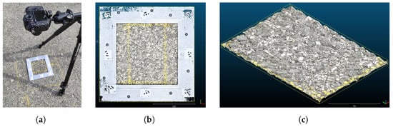
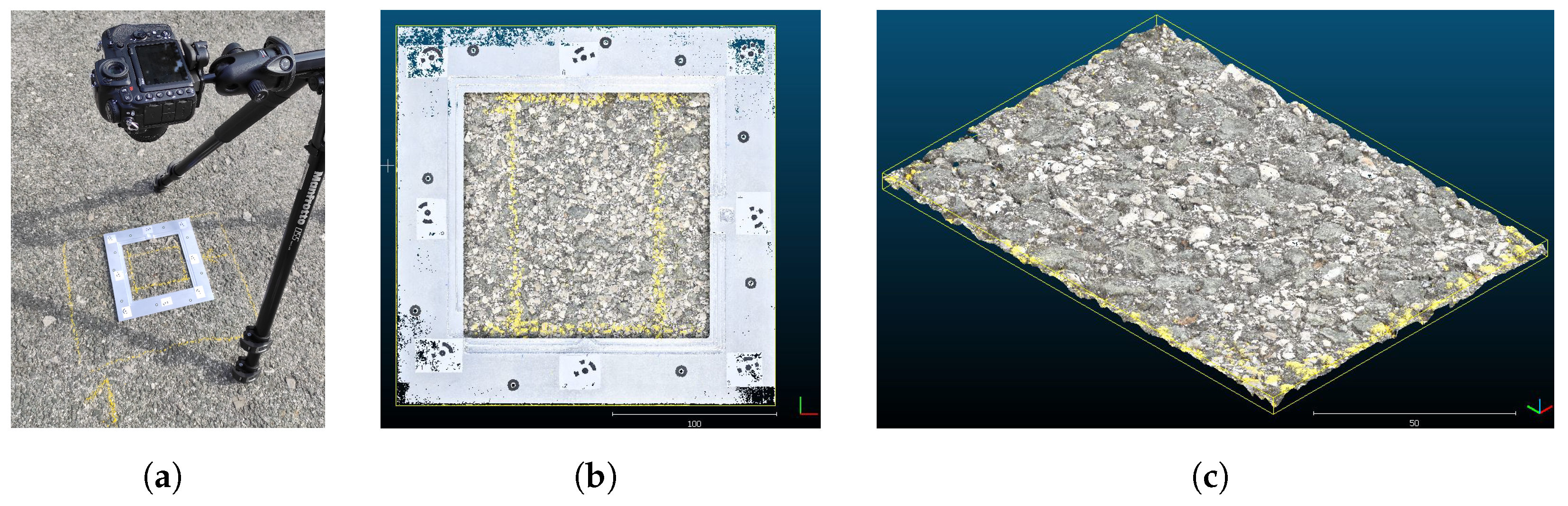
An example of data acquisition is shown in Figure 1. While the camera arrangement is shown in Figure 1a, the created pavement digital surface models (DSMs) can be observed in Figure 1b,c. Once the DSMs are generated, they were subjected to further processing in the open-source software for dense point cloud analysis Cloud Compare, v2.11.3. The DSMs of investigated surfaces were subjected to initial adjustments: leveling, so the 3D models were parallel to the horizontal plane; scaling, to correspond to millimeters unit; and filtering, so the DPC points falling outside the area of interest or relevant texture scale were removed. The final DPC model of each surface was subjected to profile segmentation to investigate the roughness properties of analyzed surfaces.
Figure 1.
(a) Pavement surface data acquisition by CROP method, with orthogonally positioned digital camera and target surface marked with reference frame; (b) digital surface model of pavement surface obtained by CROP method application; (c) an example of digital pavement surface model processed in the Cloud Compare software.
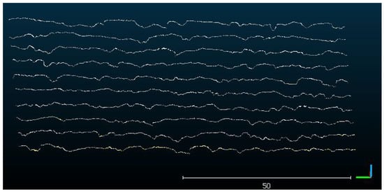
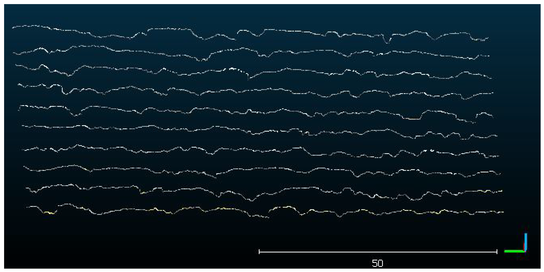
To determine the roughness properties of pavement surfaces that could be compared to the friction performance evaluated by the proposed numerical method, an analysis of profile roughness features was conducted. The profiles were segmented from the DSMs of investigated surfaces in Cloud Compare software. To segment the profiles, it has been necessary to define a segmentation area, a segment orientation, a segment length (i.e., profile length), and a lateral distance and thickness of the segmented DPC sections. The segmentation area was equal to the pavement surface area inside the reference frame and the segments were oriented to be parallel to a horizontal x-axis. The length of the segment in the x-direction was set to be , corresponding to the profile’s length for the calculation of the traditional pavement texture indicator mean profile depth (MPD) following the EN ISO 13473-1 [45] standard norm. The segments’ lateral distance was set to , so that each investigated surface was described by ten profiles, as depicted in Figure 2.
Figure 2.
A screenshot from the acquisition software provides a visualization of the profiles sampled and extracted from the digital surface model, cf. Figure 1, with defined segmentation properties: profile length is , while lateral distance between two consecutive samples is .
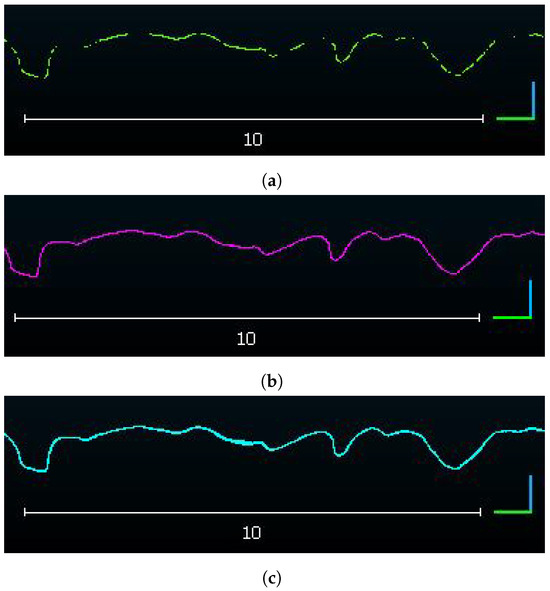
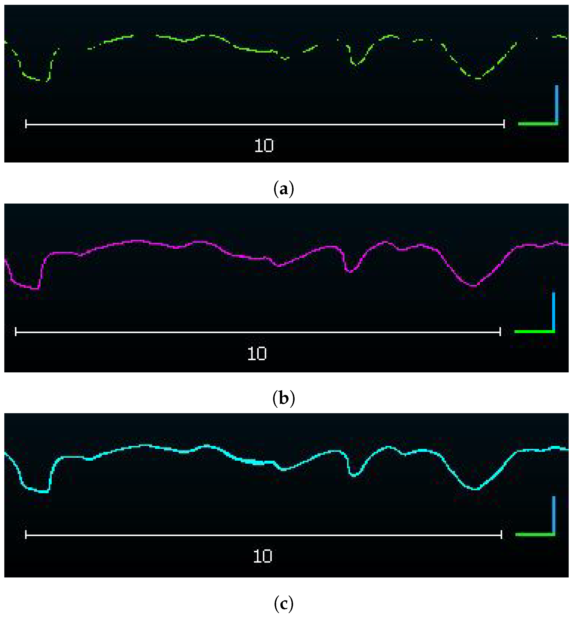
The depth in the direction orthogonal to the average surface mean plane of the segmented section was set to be , selected after the comparison of profile’s number of points for different section depth values settings. This value determines the width of the DPC segment from which the profile is created. If the selected depth values were too wide, the profile would consist of points having a single x coordinate and multiple z coordinates corresponding to the same x value. This would require dataset interpolation to obtain a 2D profile and such approximation could influence the true geometry of the surface. On the other hand, for a too narrow section depth, the number of points in a profile would not be sufficient to properly describe all roughness features as such profiles would have gaps, requiring, again, extrapolation and true roughness features approximation. An example of a profile segmented with three different section depths is given in Figure 3, obtained from the Cloud Compare software as result of the DPC data analysis.
Figure 3.
(a) Profile with section thickness equal to ; (b) profile with section thickness equal to ; (c) profile with section thickness equal to .
For a selected section depth of , the obtained profiles were shown to have an average point-to-point distance in the horizontal direction below . This value implies that extracted profiles have sub-millimeter resolution in the horizontal direction, which enables the roughness features analysis on both micro- and macro- texture scales relevant for the analysis of pavement friction phenomenon. The profiles extracted with the previously described settings in the segmentation procedure had roughly points on average. The exact number of points in each profile differs due to the morphology varieties of inspected surfaces in the positions where the profiles were segmented. For the purpose of roughness features comparison of extracted profiles, all profile points coordinates were converted from a relative to an absolute reference coordinate system so that each profile starts with a point having x coordinate equal to zero, while height coordinates were adjusted so that the minimum height value was set to zero. After the profiles’ coordinates were corrected, the adjusted profiles were imported to Mountains Map, v9.0 Lab Premium software, for analysis of the roughness features. The software enables automatic calculation of profile’s texture roughness features based on the EN ISO 21920-2 [46] standard. Roughness features can be calculated on profiles with or without scale separation, a feature that enables the exclusion of specific texture scales, if desired. In this research, no scale separation was applied and the texture parameters were determined on primary profiles containing both the relevant texture scales. To remove any remaining profile vertical slope, the profiles were automatically leveled to a horizontal plane. A Gaussian S-filter was also applied to the leveled profiles to remove the elements in the lateral direction which were not below a threshold of . In this way, the profile dataset was de-noised, while the relevant profile points within the defined horizontal resolution of were preserved.
Profile related roughness parameters were selected from the group of amplitude- or height-related parameters and feature parameters group, defined in the EN ISO 21920-2 standard. They are the most common non-standard roughness parameter groups explored in pavement texture analysis in relation to frictional performance [47,48,49,50]. The amplitude parameters are a sub-group of field parameters, related to the full length profiles and calculated from the profile heights . Feature parameters are calculated for a given section of a full length profile, describing amplitude or wavelength features of profiles’ sections within specific section lengths. Additionally, the traditional pavement texture profile-related parameter MPD was calculated for the analyzed profiles to compare its values to the values of the obtained non-standard parameters. Table 1 provides an overview of the roughness parameters calculated for the analyzed profiles, with a description of their physical meaning.
Table 1.
Profile roughness parameters determined by following EN ISO 21920-2 standard.
2.2. Profile Selection for Numerical Simulations
The aim of the research is to assess if texture roughness features calculated from the pavement surface profiles can be directly correlated to their friction response. For this purpose, three profiles were selected arbitrarily from the database, characterized by different values of calculated texture parameters, extracted from three pavement surface models obtained by the CROP method. The surfaces were previously chosen for their friction performance after a standard pavement friction measurement campaign performed with the aid of a static skid-resistance tester (SRT), test EN ISO 13036-4 [51]. This device is used for the measurement of the low-speed friction performance of pavements based on the pendulum principle [1]. The obtained friction values are expressed as SRT, a dimensionless number ranging from 0 to 150, where higher values indicate better friction performance of the inspected surface.
Hence, three surfaces selected from the database showed different measured values of SRT: surface P06 exhibited SRT of , surface P12 SRT was and, for surface P20, the evaluated SRT was . To be able to compare the roughness properties of the surfaces evaluated by the SRT device, the CROP method was later applied on the exact same surface area. The size of the inspected surface was , corresponding to the sliding distance of the pendulum’s skid and the skid’s width. The analyzed profiles were selected from the central part of the surface model, where the CROP method verification procedure achieves its best accuracy. All profiles were extracted from the DSMs by following the same procedure as described in the previous section, with the following resulting profile properties: profile length and profile resolution , obtained with a low-pass filter of .
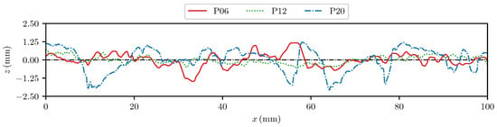
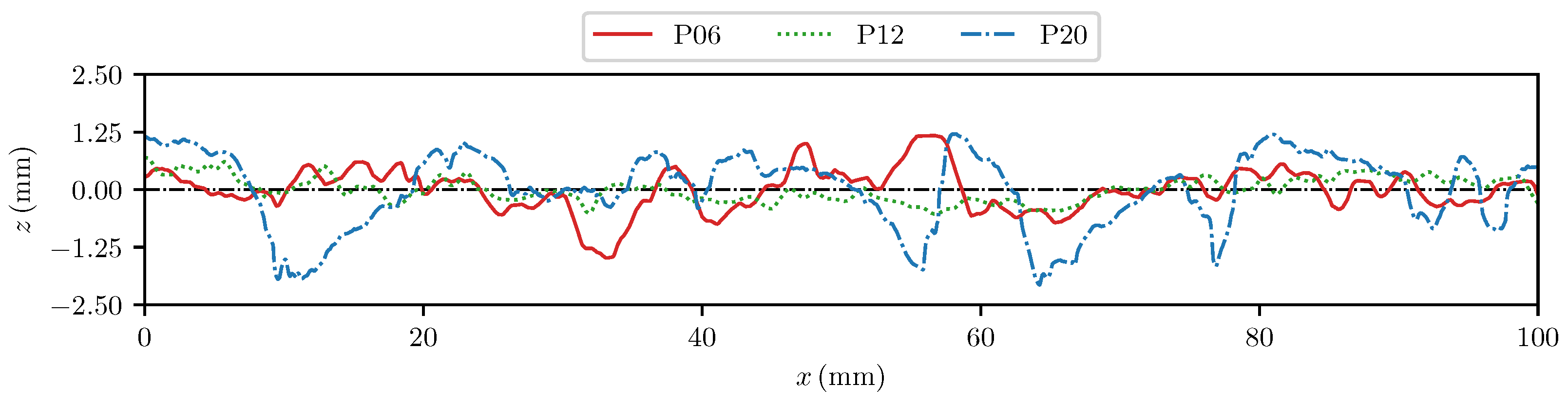
The geometry of the selected profiles is shown in Figure 4 and the values of the roughness parameters are collected in Table 2. The profile P12 has the lowest values of roughness parameter in most of the amplitude and feature parameter groups. The exception are values for and , which are related to the profile’s morphology in the horizontal direction. The traditional texture parameter for the P12 profile is the lowest, while it is the highest for the P20 profile.
Figure 4.
Elevation fields of selected profiles. The black dash–dotted line marks the zero mean elevation.
Table 2.
Measured friction values expressed in SRT and calculated profile roughness parameter values for three analyzed profiles; all roughness parameter values are expressed in .
Profile P20 obtained the highest values for all calculated parameters, in coincidence with the highest value determined for the surface from which this profile was segmented. However, the measured friction values are surface-related and therefore cannot be a reliable representation of a profile’s roughness characteristics analyzed in this work. Amplitude parameters and , calculated as mean height values for the full profile length, showed less variation in values among profiles in comparison to feature parameters describing the peak profile features, such as or . The highest variation of parameter values was obtained for the profile element parameter, characterizing the maximum profile element height.
Considering the obtained values of roughness parameters calculated for the three segmented profiles, it can be concluded that the profiles have significantly different morphologies.
3. Finite Element Computational Framework
3.1. Interface Model
The computational framework to predict the frictional response given the roughness geometries and the viscoelastic material properties is based on the MPJR interface finite elements pioneeringly proposed in [40]. A first extension to viscoelastic contact between sinusoidal profiles is proposed in [41].
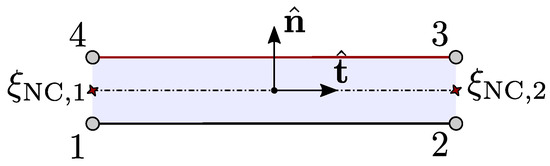
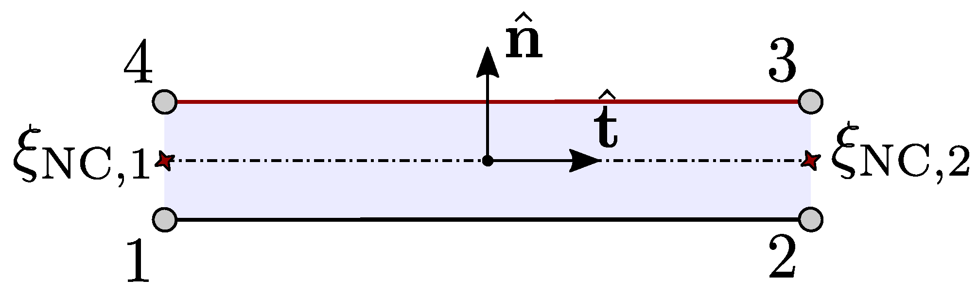
The kinematics of the element is shown in Figure 5. A vector of unknown horizontal and vertical nodal displacements, , is introduced for the evaluation of the gap function across the interface that reads:
where is a linear operator that computes the relative nodal displacements across the interface in horizontal and vertical directions, is a matrix that collects standard first-order shape functions and is a rotation matrix that maps the gap function from a local reference system, aligned with the element, to a global reference frame, where and are the unit tangential and normal vectors aligned with the element centerline and still evaluated in .
Figure 5.
Kinematics of the 2D quadrilateral MPJR element.
A correction in the nodal vector is performed by hard coding the position of the two upper nodes and to match the actual position of the rigid rough surface considered. The result of this operation is a corrected gap function whose normal component describes the kinematics of the real geometrically complex problem, now reading as
Finally, the contact tractions can be evaluated, e.g., with a standard penalty approach governed by a penalty parameter ,
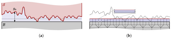
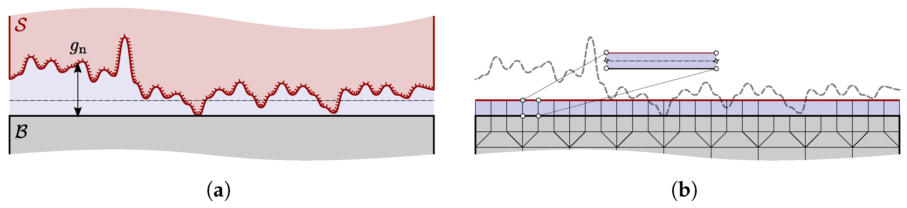
A sketch of the whole process is qualitatively shown in Figure 6 below.
Figure 6.
(a) Original problem setting; (b) discretized framework.
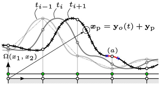
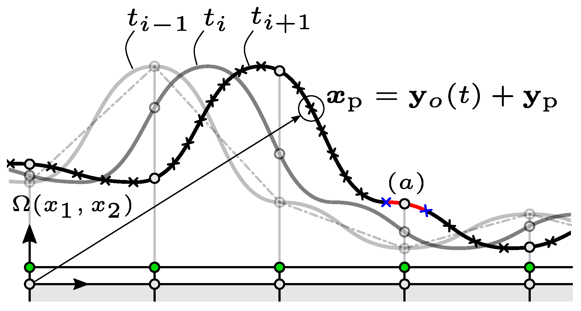
In the current study, the introduced MPJR approach is extended with an additional feature that allows one to consider a relative finite sliding involving a rough profile expressed as a set of discrete elevations over a viscoelastic body.
It is possible to express, considering the rough profile as rigid and subject to a prescribed relative motion on top to the viscoelastic substrate, the relative position of the viscoelastic body and the sliding profile for each time step.
The sliding viscoelastic body, hereinafter labeled as skid, is modeled as a rectangular domain in the reference frame , set in correspondence of the skid’s top-left corner and with the axis aligned to its top side. The analysis is developed over a time window and is divided in two main phases: a Phase I involving vertical loading, in which the rough profile is pressed against the skid, and a Phase II, where a horizontal velocity is imposed, which determines the sliding motion.
Sliding is supposed to take place between the rough profile and the top side of the skid, with the rough profile moving in accordance with a predefined rigid translating act of motion characterized by a given horizontal and vertical velocity. As stated in Section 2.2, every profile geometry is stored as a set of discrete points , whose first coordinate is set so that, considering that a local reference frame fixes with the rough profile, the first point of the ensemble is characterized by . At , the rough profile makes contact with the skid at its minimum point only, without exerting any contact pressure. In the skid’s global reference frame, the position of each point of the rough profile can be then expressed as .
To reproduce the contact conditions, an array of MPJR finite elements is defined over the skid’s top side, where, in accordance with the MPJR paradigm, the lower pair of nodes is tied to the FEM discretization of the skid’s boundary, while the normal gap is corrected to account for the variation of the position of the rough profile, Figure 7.
Figure 7.
Nodal elevation update procedure under finite sliding.
The nodal coordinate mapping of the rigid indenter during finite sliding is shown in Figure 7 for a generic node labeled , which undergoes the imposed kinematics. At each time step, the elevations at each MPJR interface node are updated accordingly. Since the height field is a discrete set of data points, a cubic spline interpolation is performed before running the simulation to determine the interpolation coefficients for all the intervals between and and, for every point i, are stored beside the initial profile’s horizontal position and elevation. The correct elevation value is then inferred identifying the closest trailing and leading correspondent points from the profile’s set. Once they have been identified, the correct elevation value is retrieved evaluating the interpolation in correspondence of the horizontal position of the interface finite element’s node.
To allow considering any horizontal velocity, the identification of the neighboring points is performed at each time step. To make the procedure computationally fast, the elevations are stored as an ordered list and a convenient binary search algorithm can be enforced to solve the problem. For each node, this operation must be carried out only once to identify the trailing point, while the leading point is the following one. Once the elevation of the rough profile in correspondence of the interface node under examination has been carried out, its value is used into the expression of the corrected normal gap, cfr. Equation (2), Equation in [41], and the resulting corrected gap can be employed to restore the true contact condition of the original problem.
3.2. Rheological Model for Rubber
For engineering applications, typically at least three terms in the Prony series are required to yield meaningful stress analysis predictions. In our case, the classic expression for the Young’s relaxation modulus has been employed:
The rheological properties of the material can be investigated in the frequency domain performing a Fourier transform of the relaxation modulus defined in Equation (4). The complex modulus in the frequency domain reads as
Starting from the complex modulus, the storage modulus can be defined as the real part of Equation (5), and it describes the ability of the material to store elastic energy. The loss modulus is defined as the imaginary part of and describes the part of energy which is dissipated as heat as the material is subjected to deformation.
To consider a realistic response to identify, the material model employed in [17,52], which corresponds to Styrene Butadiene Rubber (SBR) acquired during an experimental campaign performed at the German Institute for Rubber Technology, has been fitted using Equation (4).
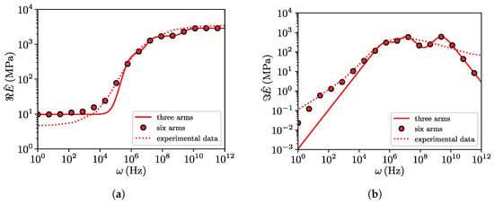
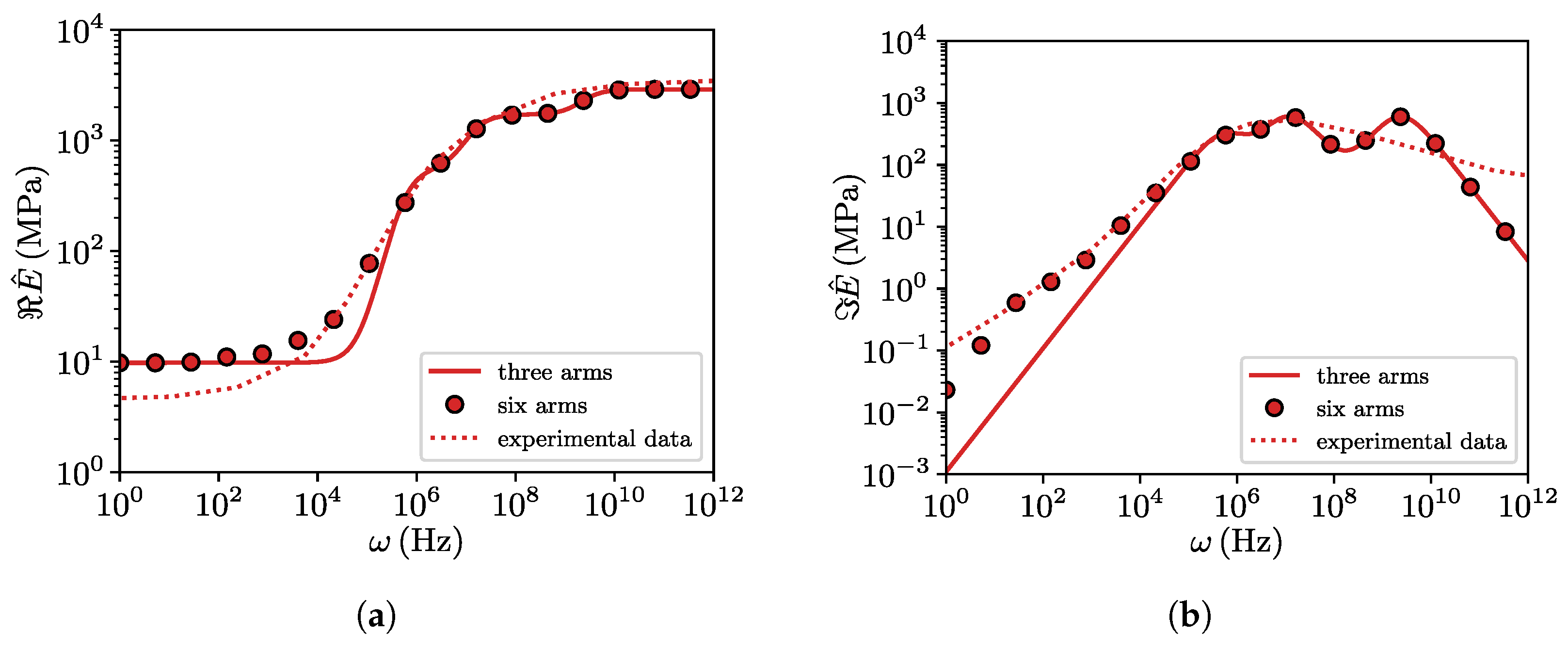
A comparison between our model and the model employed in the two aforementioned studies is depicted in Figure 8. Considering terms in the Prony series, the experimental response is reasonably well captured with a reduced complexity as compared to the reference model used in previous work with six arms.
Figure 8.
Storage (a) and loss (b) moduli for the three arms model used in this study as compared to the six arms model and experimental data from [17].
Viscoelastic model parameters are collected in Table 3.
Table 3.
Mechanical parameters for the three arms Maxwell Model.
3.3. Computation of Friction Due to Hysteresis
Assuming a linear viscoelastic body pressed against a rough profile and sliding over it under the action of a tangential load, and neglecting adhesive and Coulomb frictional effects, the contact tractions will always be orthogonal to the deformed surface. In the framework of a linear theory, a global time-varying horizontal contact force can then be determined via a geometric relation, as the integral of the projection of the normal contact tractions over the surface gradient . If is the overall time-varying vertical reaction force, a global averaged coefficient of friction can then be defined as
An analytical expression can be derived for Equation (6) for the very simple case of a viscoelastic layer characterized by a single relaxation time . If it makes full contact with a sinusoidal profile of wavelength and amplitude a, under the action of an imposed vertical far-field displacement , and slides over it with constant velocity v, the average coefficient of friction is
where is the excitation frequency and and are the long-term and the instantaneous elastic modulus of the material, respectively. From this preliminary simple model, an important property of the viscoelastic coefficient of friction can be deduced, i.e., its marked dependency on the sliding velocity v. The maximum value of is reached when the system is excited with a frequency . In a more general scenario, characterized by additional viscoelastic terms or partial contact, no closed form expression can be derived and the mean value of the hysteretic friction coefficient must be evaluated numerically according to Equation (6).
4. Benchmark Test: Sinusoidal Indenter
In this section, a first set of numerical experiments is performed to analyze the sliding of a linear viscoelastic block of dimensions and over a rigid sinusoidal shape. The profile is characterized by a wavelength and amplitude . The results in terms of and are then compared with Equation (7) and benchmarked against the results presented in [52].
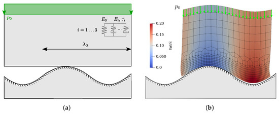
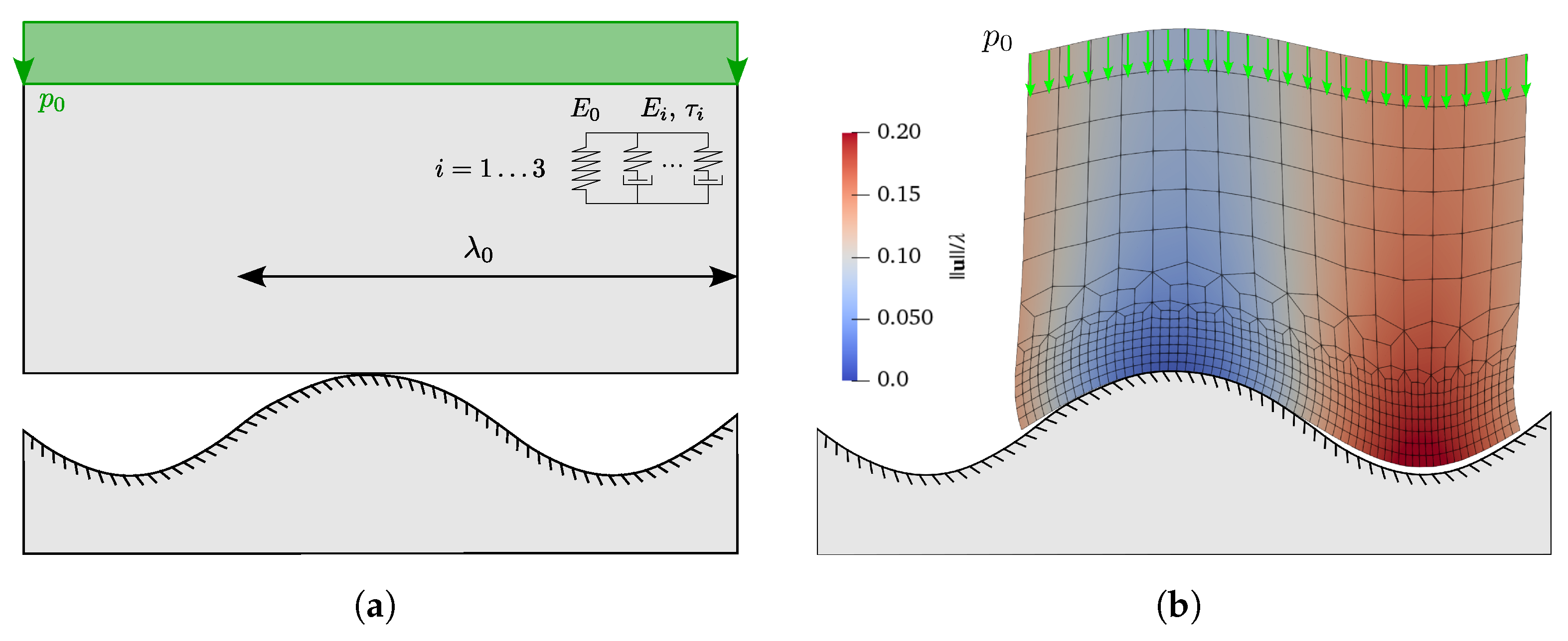
The domain is discretized by standard linear quadrilateral elements, while an array of MPJR interface finite elements is placed in correspondence of the contact interface and stores the shape of the moving sinusoidal profile. The FE mesh is refined at the contact side by means of an increasing number of elements with increasingly smaller size. The sketch of the problem under examination is depicted in Figure 9a, together with the typical mesh arrangement employed shown in a snapshot of a simulation run, Figure 9b.
Figure 9.
(a) Sketch of the problem under examination, where a rectangular viscoelastic block is, in a first moment, pushed against a rigid sinusoidal profile of period by a uniform pressure , and then forced to slide under the action of a prescribed velocity; (b) excerpt from numerical simulation at a selected representative time step. Solution is displayed in terms the contour plot of normalized displacement magnitude.
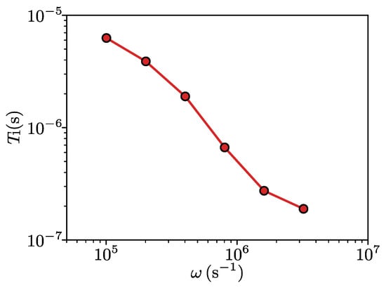
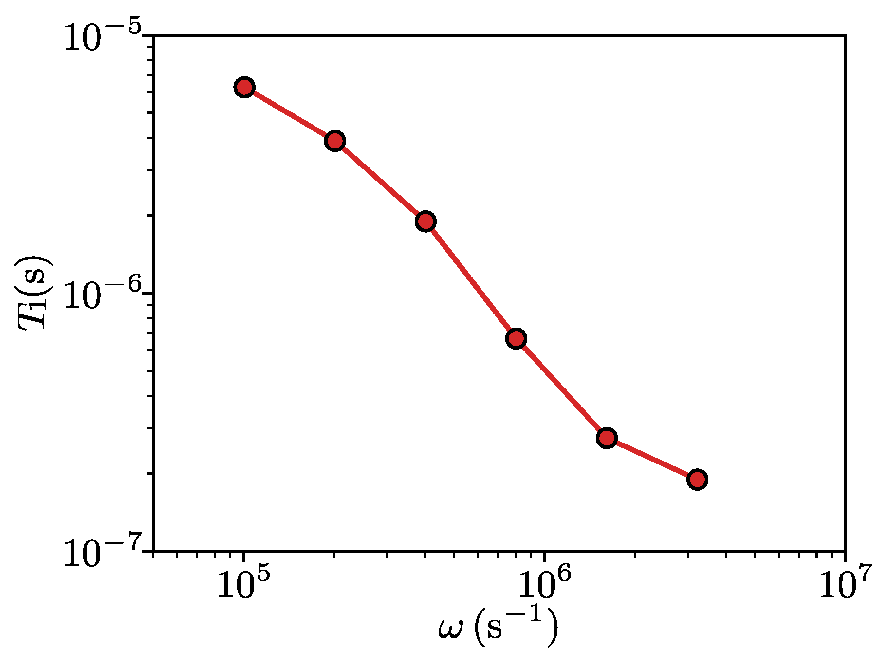
During Phase I, a uniform vertical pressure has been applied in an overall time , estimated according to the criterion discussed in [52] and necessary to limit the propagation of spurious undesired viscous effects from Phase I to Phase II. The optimal value has been estimated for different values of , see Figure 10.
Figure 10.
Optimal values for the duration of the vertical loading phase for different values of excitation pulsation .
During Phase II, a constant value of sliding velocity is considered, where the duration of the simulation has been determined by the overall sliding length necessary to correctly evaluate , a condition which is fulfilled by the full development of steady-state sliding conditions. For each time step, the variation of the profile geometry is correctly captured by the method, and the number of time steps employed in the sliding phase is such that an advancement of the block on the profile of takes place for each time increment, where coincides with the number of interface finite element used to discretize the interface and is the distance between two consecutive points at which the height is sampled. If the total sliding distance is then expressed as a multiple of the profile wavelength, the number of time steps necessary to cover the required distance results then in .
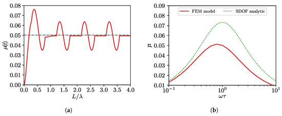
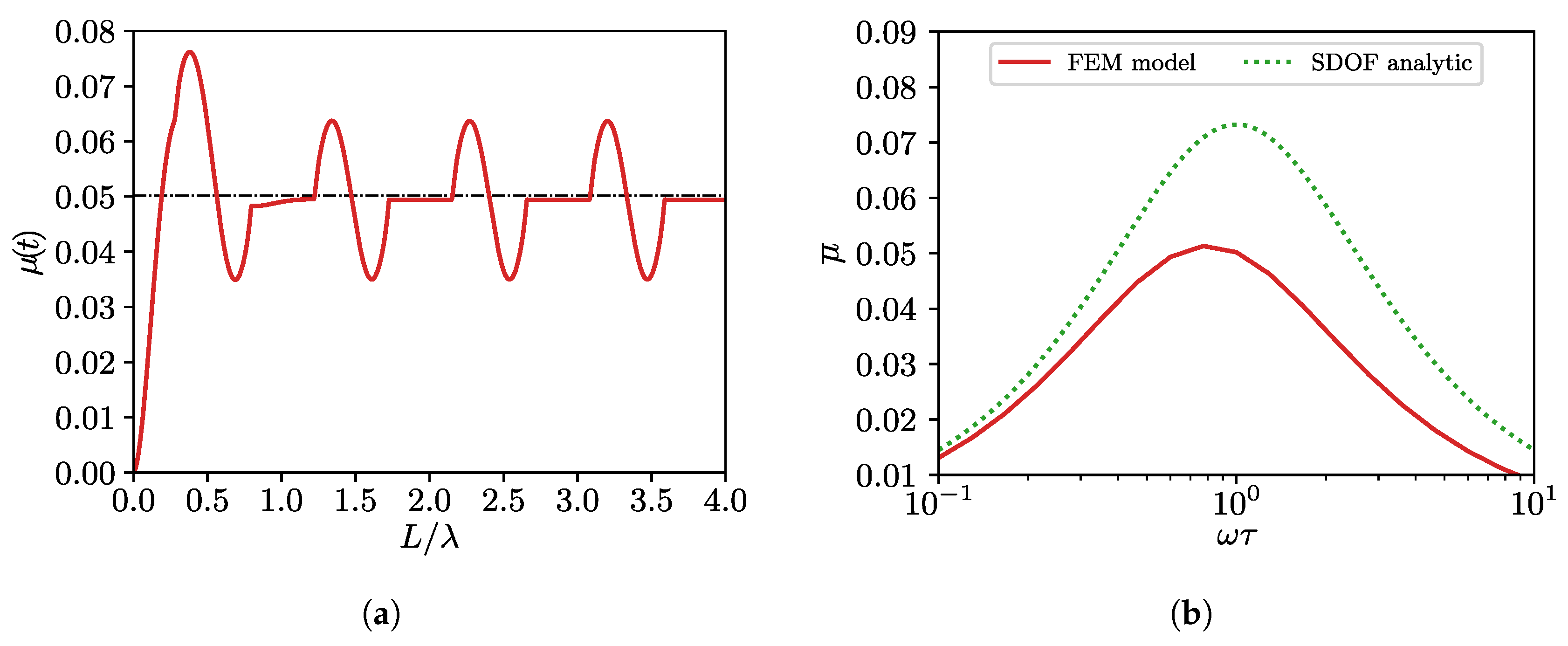
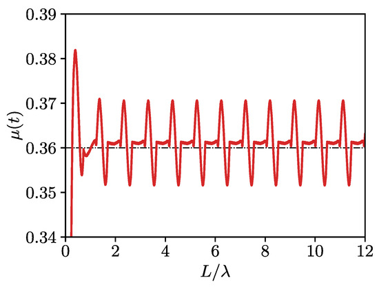
Periodic boundary conditions are enforced in correspondence of the two vertical sides of the block. The linear viscoelastic material employed for the test is characterized by a single relaxation time, with the following mechanical properties: , , , and . Different values of the applied velocity have been tested, logarithmically centered around the critical value identified by , i.e., . On the other hand, has been imposed to be correspondent to the most demanding condition, i.e., to the highest sliding velocity of . Results are plotted in Figure 11a in terms of , for the case . The results of the averaged value are plotted in Figure 11b for each velocity, together with the values provided by Equation (7). From the comparison, we clearly observe that the single degree of freedom (SDOF) analytic solution underestimates the friction coefficient as compared to the FEM prediction which accounts for the appropriate deformability of the system. The sliding velocity corresponding to the maximum friction coefficient is also shifted towards lower values in the FEM prediction.
Figure 11.
Benchmark test: friction coefficient for different sliding velocities over a sliding distance . (a) Instant value of the friction coefficient at the critical sliding speed, the black dash–dotted line represents the average value of the friction coefficient during the sliding phase; (b) averaged values of the friction coefficient for different applied velocities.
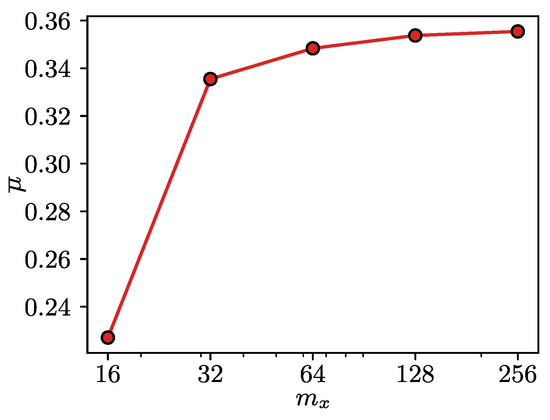
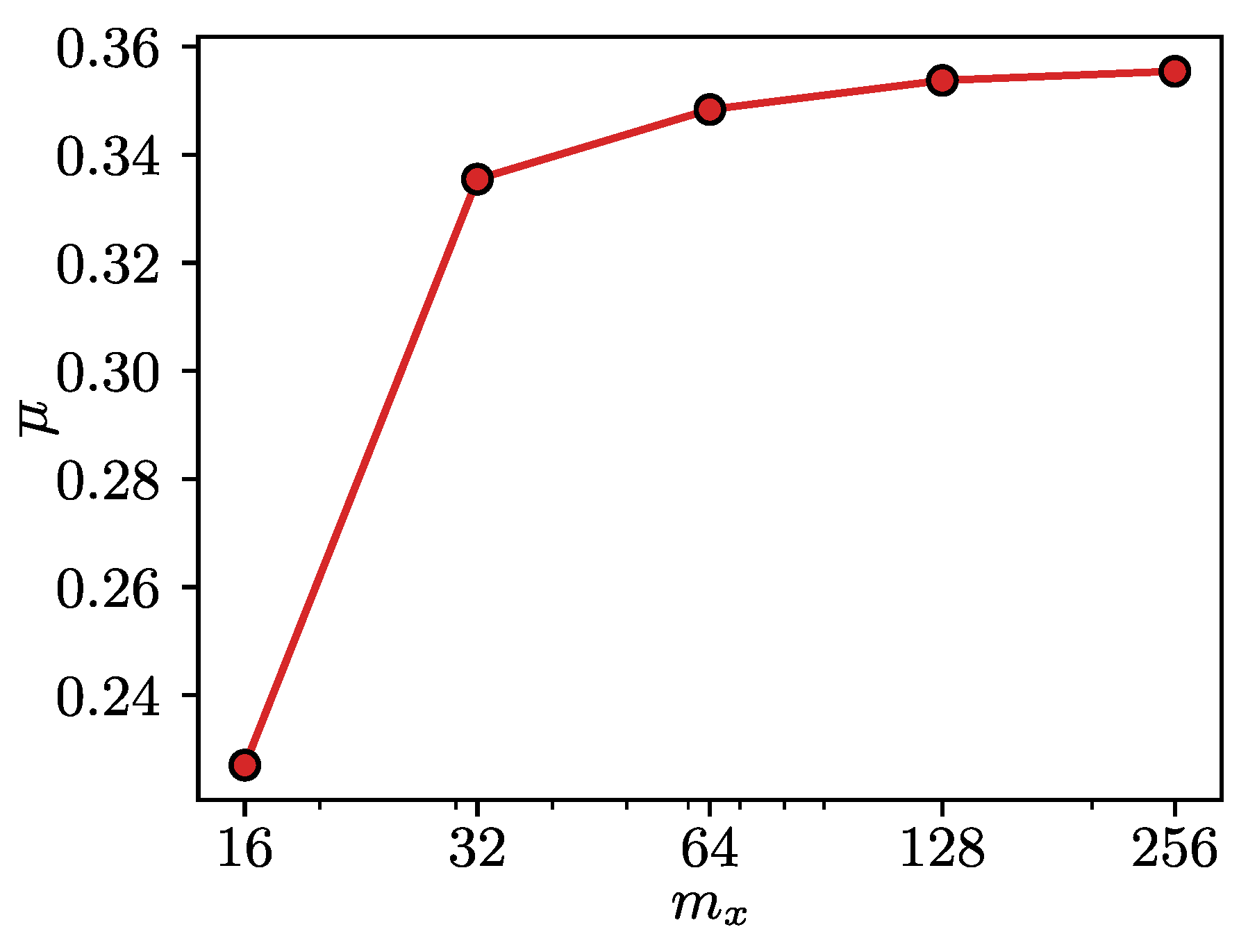
A mesh convergence analysis has been performed by increasing the number of interface finite elements that discretize the sinusoidal profile. Concurrently, different values of the penalty parameter have been tested. The results of the convergence study are shown in Figure 12 for , 32, 64, 128 and 256 interface finite elements. The contact penalty parameter has been increased until the resulting traction field was not affected anymore by further increases, resulting in a value of , with h being the domain’s height. In all the subsequent simulations, a value of interface elements per wavelength has been employed, since further refinements did not result in any appreciable accuracy gain in terms of . Numerical experiments have shown that the zone with refined mesh in the depth direction must be at least twice the size of the coarsest element in the mesh.
Figure 12.
Convergence of the average friction coefficient for different interface discretization and .
In a second test, the same simulation setting has been considered, but with a viscoelastic model featuring three terms. The material parameters are those identified in Section 3.2 and listed in Table 3. Considering the same applied normal pressure and a velocity equal to , close to the critical value, the plot of is shown in Figure 13. A direct comparison with the average value found in Ref. [52], Section 6.1, Fig. 12 for the case is superimposed with a black dashed–dotted line in the same figure.
Figure 13.
Sliding test for the imposed velocity causing a high dissipative effect, for an applied pressure of . The corresponding average value from [52] is superposed as a black dash–dotted line.
5. Advanced Simulations: Rough Profiles
5.1. Problem Set-Up
In this section, the hysteretic frictional properties of asphalt pavement surfaces are investigated using the real profiles acquired with close-range photogrammetry. Given the high resolution of the sampled profiles, using the same interface FE resolution leads to a very high computational cost. The effect of introducing a down-sampling of the profile is therefore checked in a first preliminary test. For every profile, sub-profiles have been extracted by collecting one point every nodes, with , 2, 5, and 10, respectively. The case of corresponds to including all the experimental elevations. The different values of correspond to , 256, 128, and 64 interface finite elements, respectively.
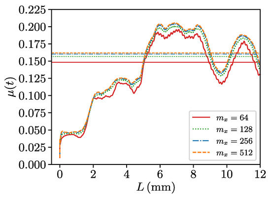
Results in terms of the simulated for the four different down-sampled resolutions are shown in Figure 14, for a sliding test up to a length of and an applied velocity of . A value of () interface finite elements instead of 512 gives very close to that of the finest resolution, both in terms of time variation and average value of the time window (shown with straight lines), and it is therefore adopted as the preferred resolution for the subsequent simulations.
Figure 14.
Simulated for different down-sampled profiles.
Since the duration of Phase I is an important parameter to guarantee a rapid extinction of the transient period during the horizontal sliding, special care must be taken for its evaluation. For a generic rough profile, a closed form expression is not available and it is not possible to follow the same strategy as for the sinusoidal profile. Nonetheless, a limiting value for the excitation frequency can still be identified if we consider the hypothetical profile with the shortest wavelength that can be taken into account given the discretization of the block’s interface. If we consider this harmonic profile as a sampled time signal, then the shortest wavelength that can be sampled corresponds to its Nyquist frequency, i.e., two times the sampling interval, which in turn is equal to , where is the distance between two sampled points. If we now consider these values for a specific sliding velocity, the corresponding maximum durations of the normal loading phase that minimize the transient regime during the sliding process can be estimated. For the chosen discretization level of and the highest velocity tested, is computed and employed in all the simulations.
A range of different sliding velocities is applied during Phase II to all the selected profiles. For each of them, twenty different values have been sampled on a logarithmic scale centered around , and within the range and . The value of has been chosen to approximately resemble the standard sliding velocity usually employed in the experimental British Pendulum friction tests (BPT) [53], while the bounding values of the range have been designed to be far enough from the critical speed, in order to clearly assess the maximum value of and its sensitivity to the changes in skid’s velocity. A sliding length coincident with the complete development of the available profiles has been used in every case analyzed, leading to an overall value , resulting, in turn, in a ratio with the skid length of .
A value of for the vertical applied pressure has been employed for all the three profiles herein analyzed.
5.2. Results and Discussion
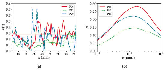
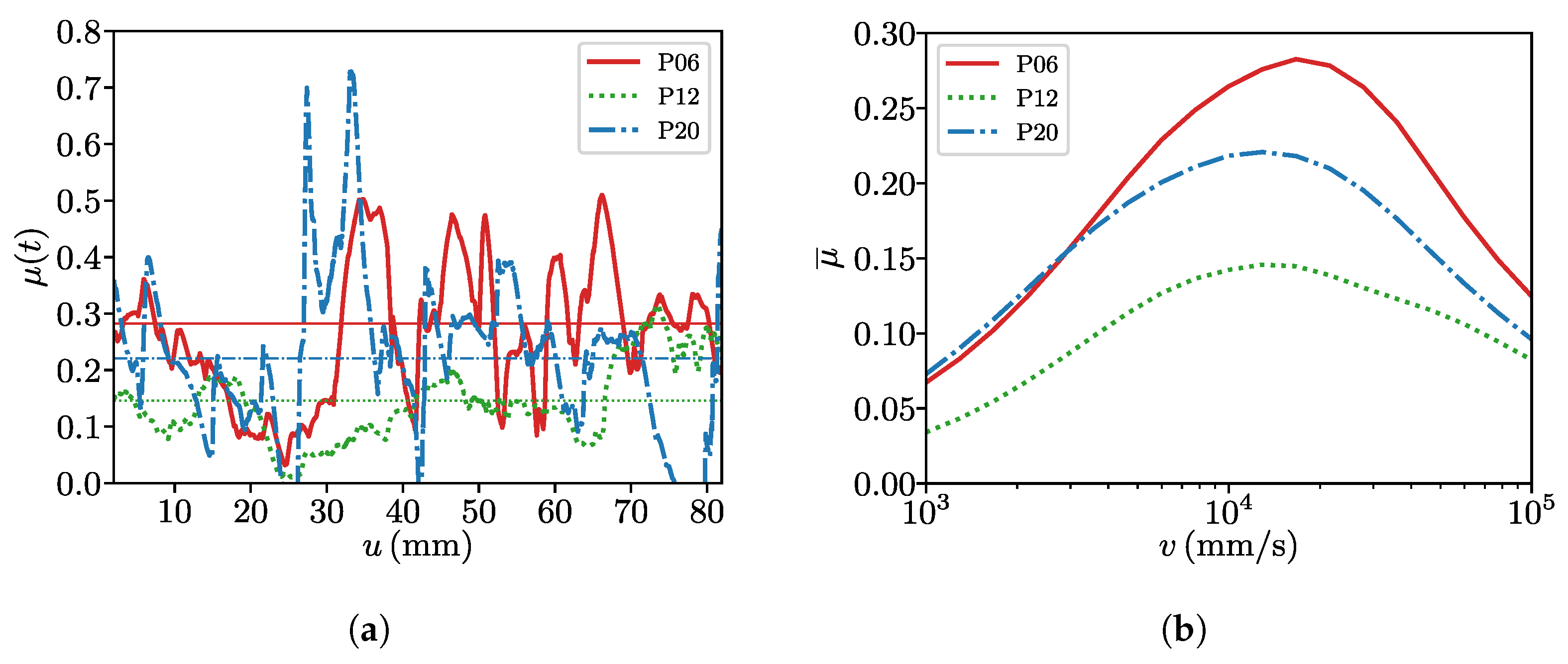
Simulation results are shown in Figure 15. Figure 15a shows the instant values of the viscoelastic friction coefficient for the three profiles in correspondence of the velocity which gives the highest . It can be noticed how the average magnitudes of the values are in line with the mean values reported in [24]. Figure 15b shows the average values of the viscoelastic coefficient of friction for all the simulated sliding velocities, again for each profile. The critical value for the velocity can be identified from the maximum friction coefficient, which starts around for P12 and then increases for P20 and P06.
Figure 15.
Simulated viscoelastic coefficient of friction for real rough profiles. (a) Instant value of the viscoelastic coefficient of friction for the critical value of the sliding velocity, the respective average values are superposed as horizontal lines; (b) average value of the viscoelastic coefficient of friction vs. sliding velocity.
The maximum instantaneous values of for the three profiles employed correctly reproduce the qualitative link between surface geometry and viscoelastic friction generation. Specifically, the maximum instantaneous coefficient of friction for each profile P20, P12 and P06 scales consistently with the geometrical roughness descriptors , , , , , , and from Table 2, which are all related to the profiles’ vertical dimensions. This is physically sound, since peak friction events are governed by local contact conditions as steep asperity slopes and large peak-to-valley distances. The model correctly captures the local, high-frequency viscoelastic response of the rubber to the sharpest topographic features.
On the other hand, the average coefficient of friction , shown in Figure 15b for the three profiles and all the sliding velocities analyzed, does not reproduce the same trend as the experimental SRT values, cf. Expression (8). Instead of the same monotonic correspondence obtained from the experimental tests, the simulated average gives , thus not matching the SRT ordering.
These results suggest that a local and instantaneous friction response might be closer to the SRT number than a spatially or temporally averaged one, since they are both localized and short term responses, while integrates over the entire profile length, including valleys and long-wavelength regions that are not sampled by the pendulum. In this sense, is more sensitive to the full distribution of local sliding velocities and strain rates encountered along the whole profile, which excites a broader range of the rubber’s viscoelastic relaxation times. The maximum values, being dominated by few extreme asperities, samples a narrower frequency band, making it more directly comparable to the SRT measurement.
These considerations still do not explain the mismatch between the numerical ranking and the SRT ranking related to the profiles P06 and P12. This points to an additional physical effect that the simulation is probably not resolving. The SRT test reflects the real physical continuous surface, including wavelengths at scales finer than the numerical digitized profile, which might carry a contribution that the viscoelastic model can not capture. To back this claim, it can be observed that profile P12 presents the highest values of and , which both describe profile element spacing in the horizontal direction. If this information is combined with the smallest descriptors for vertical amplitude, we can conclude that the numerical profile P12 is characterized by asperities that are both smaller and less frequent, and this might result in a penalization of both and .
Further analyses should be devoted to strengthen the aforementioned interpretation of the results, which offer an underlying physical trend which is correct, but that is missing a deeper statistical insight. Closing this gap relevant for uncertainty quantification requires more profiles to be taken into consideration to give this comparison the proper statistical weight.
6. Conclusions
We extended the MPJR approach to address the complexities of tire–pavement interaction by simulating the hysteretic frictional response of real pavement texture roughness features. By embedding detailed pavement profile models acquired with close-range photogrammetry into the finite element method, the procedure allows advanced contact mechanics simulations.
The findings of the study suggest that the MPJR approach is accurate and practical for evaluating the hysteretic coefficient of friction, delivering values which are in line with those reported in the literature. A correlation with specific roughness parameters derived from the analysis of the profiles has been identified concerning the roughness descriptors related to the vertical dimension of the profiles. On the other hand, an exact correlation with the SRT descriptor could not be identified, possibly implying that some features captured by the experimental set-up are missing from the numerical model.
Important aspects that were left out are related to the approximation of the 3D surface with 2D profiles and the use of a small dataset. After this preliminary study, future work will build on these results by incorporating large-scale 3D analyses, featuring richer datasets that will guarantee the statistical soundness of the results.
In conclusion, the good agreement on maximum friction vs. geometric parameters confirms that the model correctly resolves local asperity-driven dissipation; while the less good agreement on average friction vs. SRT parameter reflects a mismatch in what is being measured rather than an error in the simulation itself. Closing this gap will allow practitioners to estimate the viscoelastic frictional performance of rubber pavement contacts from numerical simulations, reducing the reliance on time-consuming and costly experimental campaigns.
Author Contributions
Conceptualization, I.B., J.B. and M.P.; methodology, I.B., J.B. and M.P.; software, J.B. and M.P.; validation, I.B. and J.B.; formal analysis, J.B. and I.B.; investigation, J.B. and I.B.; resources, J.B., I.B. and M.P.; data curation, I.B.; writing—original draft preparation, J.B.; writing—review and editing, J.B. and I.B.; visualization, J.B.; supervision, M.P.; project administration, M.P.; funding acquisition, M.P. All authors have read and agreed to the published version of the manuscript.
Funding
This research received no external funding.
Data Availability Statement
The data that support the findings of this study are available from the corresponding author upon reasonable request.
Conflicts of Interest
The authors declare no conflicts of interest.
References
- National Academies of Sciences Engineering and Medicine. Guide for Pavement Friction; National Academies of Sciences Engineering and Medicine: Washington, DC, USA, 2009. [Google Scholar] [CrossRef] [Scilit]
- Kogbara, R.B.; Masad, E.A.; Kassem, E.; Scarpas, A.; Anupam, K. A state-of-the-art review of parameters influencing measurement and modeling of skid resistance of asphalt pavements. Constr. Build. Mater. 2016, 114, 602–617. [Google Scholar] [CrossRef] [Scilit]
- Guo, F.; Pei, J.; Zhang, J.; Li, R.; Zhou, B.; Chen, Z. Study on the skid resistance of asphalt pavement: A state-of-the-art review and future prospective. Constr. Build. Mater. 2021, 303, 124411. [Google Scholar] [CrossRef] [Scilit]
- Chu, L.; Cui, X.; Zhang, K.; Fwa, T.F.; Han, S. Directional Skid Resistance Characteristics of Road Pavement: Implications for Friction Measurements by British Pendulum Tester and Dynamic Friction Tester. Transp. Res. Rec. 2019, 2673, 793–803. [Google Scholar] [CrossRef] [Scilit]
- Alhasan, A.; Smadi, O.; Bou-Saab, G.; Hernandez, N.; Cochran, E. Pavement Friction Modeling using Texture Measurements and Pendulum Skid Tester. Transp. Res. Rec. 2018, 2672, 440–451. [Google Scholar] [CrossRef] [Scilit]
- Bowden, F.P.; Tabor, D. The Area of Contact between Stationary and Moving Surfaces. Proc. R. Soc. Lon. Ser. A. Math. Phys. Sci. 1939, 169, 391–413. [Google Scholar] [CrossRef] [Scilit]
- Persson, B.N.J. Theory of rubber friction and contact mechanics. J. Chem. Phys. 2001, 115, 3840–3861. [Google Scholar] [CrossRef] [Scilit]
- Popov, V.L. Contact Mechanics and Friction: Physical Principles and Applications; Springer: Heidelberg, Germany, 2010. [Google Scholar] [CrossRef] [Scilit]
- Chen, S.; Liu, X.; Luo, H.; Yu, J.; Chen, F.; Zhang, Y.; Ma, T.; Huang, X. A state-of-the-art review of asphalt pavement surface texture and its measurement techniques. J. Road Eng. 2022, 2, 156–180. [Google Scholar] [CrossRef] [Scilit]
- Li, Q.; Yang, G.; Wang, K.C.P.; Zhan, Y.; Wang, C. Novel Macro- and Microtexture Indicators for Pavement Friction by Using High-Resolution Three-Dimensional Surface Data. Transp. Res. Rec. 2017, 2641, 164–176. [Google Scholar] [CrossRef] [Scilit]
- Deng, Q.; Zhan, Y.; Liu, C.; Qiu, Y.; Zhang, A. Multiscale power spectrum analysis of 3D surface texture for prediction of asphalt pavement friction. Constr. Build. Mater. 2021, 293, 123506. [Google Scholar] [CrossRef] [Scilit]
- Edmondson, V.; Woodward, J.; Lim, M.; Kane, M.; Martin, J.; Shyha, I. Improved non-contact 3D field and processing techniques to achieve macrotexture characterisation of pavements. Constr. Build. Mater. 2019, 227, 116693. [Google Scholar] [CrossRef] [Scilit]
- Klüppel, M.; Heinrich, G. Rubber friction on self-affine road tracks. Rubber Chem. Technol. 2000, 73, 578–606. [Google Scholar] [CrossRef] [Scilit]
- Heinrich, G.; Klüppel, M. Rubber friction, tread deformation and tire traction. Wear 2008, 265, 1052–1060. [Google Scholar] [CrossRef] [Scilit]
- Yu, N.; Polycarpou, A.A. Adhesive contact based on the Lennard–Jones potential: A correction to the value of the equilibrium distance as used in the potential. J. Colloid Interface Sci. 2004, 278, 428–435. [Google Scholar] [CrossRef] [Scilit]
- Sauer, R.A.; Wriggers, P. Formulation and analysis of a three-dimensional finite element implementation for adhesive contact at the nanoscale. Comput. Methods Appl. Mech. Eng. 2009, 198, 3871–3883. [Google Scholar] [CrossRef] [Scilit]
- Wriggers, P.; Reinelt, J. Multi-scale approach for frictional contact of elastomers on rough rigid surfaces. Comput. Methods Appl. Mech. Eng. 2009, 198, 1996–2008. [Google Scholar] [CrossRef] [Scilit]
- Lang, A.; Klüppel, M. Influences of temperature and load on the dry friction behaviour of tire tread compounds in contact with rough granite. Wear 2017, 380–381, 15–25. [Google Scholar] [CrossRef] [Scilit]
- Paggi, M.; Hills, D. Modeling and Simulation of Tribological Problems in Technology; Springer: Cham, Switzerland, 2020. [Google Scholar] [CrossRef] [Scilit]
- Ziefle, M.; Nackenhorst, U. Numerical techniques for rolling rubber wheels: Treatment of inelastic material properties and frictional contact. Comput. Mech. 2008, 42, 337–356. [Google Scholar] [CrossRef] [Scilit]
- Zienkiewicz, O.C.; Taylor, R.L. The Finite Element Method—Volume 1: The Basis, 5th ed.; Butterworth-Heinemann: Oxford, UK, 2002; Volume 1. [Google Scholar]
- Brebbia, C.A. The birth of the boundary element method from conception to application. Eng. Anal. Bound. Elem. 2017, 77, iii–x. [Google Scholar] [CrossRef] [Scilit]
- Yu, M.; Wu, G.; Kong, L.; Tang, Y. Tire-Pavement Friction Characteristics with Elastic Properties of Asphalt Pavements. Appl. Sci. 2017, 7, 1123. [Google Scholar] [CrossRef] [Scilit]
- Peng, Y.; Li, J.Q.; You, Z.; Wang, K.C.P.; Yang, G. Finite Element Method-Based Skid Resistance Simulation Using In-Situ 3D Pavement Surface Texture and Friction Data. Materials 2019, 12, 3821. [Google Scholar] [CrossRef] [Scilit]
- Yu, M.; You, Z.; Wu, G.; Kong, L.; Liu, C.; Gao, J. Measurement and modeling of skid resistance of asphalt pavement: A review. Constr. Build. Mater. 2020, 260, 119878. [Google Scholar] [CrossRef] [Scilit]
- Lo, J.W.K.; Fwa, T.F.; Oey, L.M. A finite element study of the friction between tires and rough pavement surfaces. Transp. Res. Rec. 2007, 2008, 99–107. [Google Scholar] [CrossRef] [Scilit]
- Fwa, T.F. Skid resistance determination for pavement management and wet-weather road safety. Int. J. Transp. Sci. Technol. 2017, 6, 217–227. [Google Scholar] [CrossRef] [Scilit]
- Hermange, C.; Oder, G.; Le Chenadec, Y.; Le Touzé, D. A 3D SPH–FE coupling for FSI problems and its application to tire hydroplaning simulations on rough ground. Comput. Methods Appl. Mech. Eng. 2019, 355, 558–590. [Google Scholar] [CrossRef] [Scilit]
- Srirangam, S.K.; Anupam, K.; Scarpas, A.; Kasbergen, C.; Kane, M. Safety Aspects of Wet Asphalt Pavement Surfaces hrough Field and Numerical Modeling Investigations. Transp. Res. Rec. J. Transp. Res. Board 2014, 2446, 37–51. [Google Scholar] [CrossRef] [Scilit]
- Tang, T.; Anupam, K.; Kasbergen, C.; Scarpas, A.; Erkens, S. A finite element study of rain intensity on skid resistance for permeable asphalt concrete mixes. Constr. Build. Mater. 2019, 220, 464–475. [Google Scholar] [CrossRef] [Scilit]
- Srirangam, S.K.; Anupam, K.; Kasbergen, C.; Scarpas, A. Analysis of asphalt mix surface-tread rubber interaction by using finite element method. J. Traffic Transp. Eng. (Engl. Ed.) 2017, 4, 395–402. [Google Scholar] [CrossRef] [Scilit]
- Wagner, P.; Wriggers, P.; Veltmaat, L.; Clasen, H.; Prange, C.; Wies, B. Numerical multiscale modelling and experimental validation of low speed rubber friction on rough road surfaces including hysteretic and adhesive effects. Tribol. Int. 2017, 111, 243–253. [Google Scholar] [CrossRef] [Scilit]
- Wagner, P.; Wriggers, P.; Klapproth, C.; Prange, C.; Wies, B. Multiscale FEM approach for hysteresis friction of rubber on rough surfaces. Comput. Methods Appl. Mech. Eng. 2015, 296, 150–168. [Google Scholar] [CrossRef] [Scilit]
- Tang, T.; Anupam, K.; Kasbergen, C.; Kogbara, R.; Scarpas, A.; Masad, E. Finite Element Studies of Skid Resistance under Hot Weather Condition. Transp. Res. Rec. 2018, 2672, 382–394. [Google Scholar] [CrossRef] [Scilit]
- Oden, J.T.; Martins, J.A. Models and computational methods for dynamic friction phenomena. Comput. Methods Appl. Mech. Eng. 1985, 52, 527–634. [Google Scholar] [CrossRef] [Scilit]
- Liu, X.; Cao, Q.; Wang, H.; Chen, J.; Huang, X. Valuation of Vehicle Braking Performance on Wet Pavement Surface using an Integrated Tire-Vehicle Modeling Approach. Transp. Res. Rec. 2019, 2673, 295–307. [Google Scholar] [CrossRef] [Scilit]
- Gert, H. Hysteresis Friction of Sliding Rubbers on Rough and Fractal Surfaces. Rubber Chem. Technol. 1997, 70, 1–14. [Google Scholar] [CrossRef] [Scilit]
- Zhu, S.; Liu, X.; Cao, Q.; Huang, X. Numerical Study of Tire Hydroplaning Based on Power Spectrum of Asphalt Pavement and Kinetic Friction Coefficient. Adv. Mater. Sci. Eng. 2017, 2017, 5843061. [Google Scholar] [CrossRef] [Scilit]
- Cho, J.R.; Lee, H.W.; Sohn, J.S.; Kim, G.J.; Woo, J.S. Numerical investigation of hydroplaning characteristics of three-dimensional patterned tire. Eur. J. Mech. Solids 2006, 25, 914–926. [Google Scholar] [CrossRef] [Scilit]
- Paggi, M.; Reinoso, J. A variational approach with embedded roughness for adhesive contact problems. Mech. Adv. Mater. Struct. 2020, 27, 1731–1747. [Google Scholar] [CrossRef] [Scilit]
- Bonari, J.; Paggi, M. Viscoelastic Effects during Tangential Contact Analyzed by a Novel Finite Element Approach with Embedded Interface Profiles. Lubricants 2020, 8, 107. [Google Scholar] [CrossRef] [Scilit]
- Ban, I. A Model for Skid Resistance Prediction Based on Non-Standard Pavement Surface Texture Parameters. Ph.D. Thesis, University of Rijeka, Faculty of Civil Engineering, Rijeka, Croatia, 2023. [Google Scholar]
- Luhmann, T.; Robson, S.; Kyle, S.; Harley, I. Close Range Photogrammetry: Principles, Techniques and Applications; Whittles: Lancashire, UK, 2006. [Google Scholar]
- Marulli, M.R.; Sorrentino, G.; Paggi, M. Multi-scale contact mechanics framework for upper palaeolithic ground stone tools. J. Archaeol. Sci. Rep. 2025, 61, 104939. [Google Scholar] [CrossRef] [Scilit]
- EN ISO 13473-1:2019; Characterization of Pavement Texture by Use of Surface Profiles—Part 1: Determination of Mean Profile Depth. European Committee for Standardization: Brussels, Belgium, 2019.
- EN ISO 21920-2:2021; Geometrical Product Specifications (GPS)—Surface Texture: Profile—Part 2: Terms, Definitions and Surface Texture Parameters. International Organization for Standardization: Geneva, Switzerland, 2021.
- Bitelli, G.; Simone, A.; Girardi, F.; Lantieri, C. Laser Scanning on Road Pavements: A New Approach for Characterizing Surface Texture. Sensors 2012, 12, 9110–9128. [Google Scholar] [CrossRef] [Scilit]
- Copetti Callai, S.; De Rose, M.; Tataranni, P.; Makoundou, C.; Sangiorgi, C.; Vaiana, R. Microsurfacing Pavement Solutions with Alternative Aggregates and Binders: A Full Surface Texture Characterization. Coatings 2022, 12, 1905. [Google Scholar] [CrossRef] [Scilit]
- Zuniga-Garcia, N.; Prozzi, J.A. High-Definition Field Texture Measurements for Predicting Pavement Friction. Transp. Res. Rec. 2019, 2673, 246–260. [Google Scholar] [CrossRef] [Scilit]
- Kogbara, R.B.; Masad, E.A.; Woodward, D.; Millar, P. Relating surface texture parameters from close range photogrammetry to Grip-Tester pavement friction measurements. Constr. Build. Mater. 2018, 166, 227–240. [Google Scholar] [CrossRef] [Scilit]
- EN 13036-4:2011; Road and Airfield Surface Characteristics—Test Methods—Part 4: Method for Measurement of Slip/Skid Resistance of a Surface: The Pendulum Test. European Committee for Standardization: Brussels, Belgium, 2011.
- De Lorenzis, L.; Wriggers, P. Computational homogenization of rubber friction on rough rigid surfaces. Comput. Mater. Sci. 2013, 77, 264–280. [Google Scholar] [CrossRef] [Scilit]
- Liu, Y.; Fwa, T.F.; Choo, Y.S. Finite-Element Modeling of Skid Resistance Test. J. Transp. Eng. 2003, 129, 316–321. [Google Scholar] [CrossRef] [Scilit]

Disclaimer/Publisher’s Note: The statements, opinions and data contained in all publications are solely those of the individual author(s) and contributor(s) and not of MDPI and/or the editor(s). MDPI and/or the editor(s) disclaim responsibility for any injury to people or property resulting from any ideas, methods, instructions or products referred to in the content. |
© 2026 by the authors. Licensee MDPI, Basel, Switzerland. This article is an open access article distributed under the terms and conditions of the Creative Commons Attribution (CC BY) license.