


Abstract
Brain tumour classifiers are often reported as near-perfect and explainable without checking patient structure or annotations. We reproduced a recent attention framework (SSPANet) on the Figshare dataset (3064 T1-weighted contrast-enhanced slices, 233 patients). Its image-level split is fully patient-leaky; every configuration exceeds 98% accuracy, which drops by 5–9 points on the patient-wise split. Under a fixed training recipe, seven attention modules stayed within ±0.63 points of the plain backbone, whereas the recipe changed accuracy by up to 4.7 points. As a case study, TG-SSPANet uses expert masks to supervise attention, train a segmentation decoder and gate evidence pooling. With ResNet50, it reached 96.8% slice-level and, averaging slice probabilities, 98.3% patient-level accuracy (84.5% if every slice had to be correct; 15% of patients had discordant slices), within the confidence intervals of simpler mask-using pipelines; its attention module added no measurable benefit. Its Grad-CAM++ maps hit the tumour in 81% of held-out slices, but this follows from its decoder by construction, not the classifier’s reasoning. After tumour inpainting, whole-slice models kept 80–86% accuracy, and shuffling the remaining tissue left 60–74%, so location, perilesional cues and tissue statistics cannot be separated. Patient-wise evaluation, same-recipe controls and mask-based faithfulness tests should precede explainability claims.
1. Introduction
Primary brain and central nervous system tumours are biologically heterogeneous neoplasms whose histological type largely determines prognosis and management [1]. Gliomas arise from glial cells and infiltrate the brain parenchyma. Meningiomas are usually extra-axial, dural-based lesions that compress rather than invade the brain. Pituitary adenomas originate in the sellar region and can disturb endocrine function and vision. Contrast-enhanced T1-weighted (T1-CE) MRI is the routine modality for detecting and characterizing these tumours. Their radiological distinction rests on features of the lesion and its immediate surroundings: location relative to the dura and sella, enhancement pattern, margins and mass effect. A clinically trustworthy computer-aided classifier should therefore base its decision on the lesion and its perilesional context, not on patient-specific anatomy elsewhere in the slice. This requirement is the biological premise of the present work.
The public Figshare dataset of Cheng et al. [2,3] has become the standard benchmark for three-class classification of glioma, meningioma and pituitary tumour. ImageNet-pre-trained convolutional neural networks (CNNs) [4,5] now routinely report accuracies above 95% on it [2,6,7,8,9,10]. Attention modules that reweight feature maps along the channel and/or spatial dimensions [11,12,13,14,15,16,17] are a popular way to push this further. They are also frequently presented as a route to interpretability, because class-activation maps (CAMs) such as Grad-CAM [18], Grad-CAM++ [19] and Eigen-CAM [20] are expected to highlight the lesion.
Hasan et al. [21] followed this path with the Strip-Style Pooling Attention Network (SSPANet), which combines Z-pool channel attention with strip pooling [16] and style pooling [17]. They reported 93% and 97% accuracy with VGG16 [5] and ResNet50 [4], and judged explanations by visual inspection. We reproduced this work end to end and identified six methodological gaps. First, the tumour masks distributed with every slice [2,3] were not used for training or for evaluating explanations, which were judged only visually (G1). Second, the image-level split leaks patients between training and test sets, which is known to inflate accuracy in 2D MRI classification [22,23] (G2). Third, a single attention module is applied at a single stage, without ablation (G3). Fourth, class imbalance is not handled (G4). Fifth, SE [11] and CBAM [12] are discussed but not evaluated (G5). Sixth, computational cost and run-to-run variance are not measured (G6).
These gaps matter because a classifier can achieve high accuracy by relying on shortcuts, such as patient identity or anatomy unrelated to the lesion, rather than on the lesion itself [24,25]. Saliency maps not validated against annotations can provide false reassurance [26,27,28].
This article is a reproducibility and evaluation study. We draw all conclusions about generalization from the leakage-free patient-wise protocol; we use the original image-level protocol only to reproduce the published study and treat it as non-held-out. Our contributions are fivefold. First, we quantify leakage: a multi-seed reproduction of the SSPANet study with two backbones and seven attention modules shows that the image-level split is fully patient-leaky and that accuracy on it is saturated. Second, we separate recipe from architecture: under a leakage-free patient-wise protocol with same-recipe controls, the training recipe changes accuracy far more than any of the seven attention modules. Third, we compare explanations with decisions: a quantitative evaluation against the expert masks, with reference maps, perturbation-based faithfulness tests [29], and location-only and inpainting controls, shows that tumour-centred explanations can coexist with decisions that still draw on information outside the lesion.
Fourth, we present a mask-guided case study. TG-SSPANet uses expert masks to supervise multi-stage strip–style attention (TGSA), train a light segmentation decoder, and gate where the classifier pools its evidence (tumour-focused pooling, TFP). We compare it with simpler mask-using pipelines: a two-stage ROI-crop classifier, an oracle ground-truth gate, and a Y-Net-style joint model [30]. It illustrates what mask supervision does and does not achieve, and a patient-wise ablation separates the contributions of the attention module, the decoder and the pooling gate. Fifth, for statistics and reproducibility, we report patient-clustered confidence intervals, patient-level accuracy, descriptive corrected resampled tests and calibration, and we release all code, splits and per-image predictions. Figure 1 summarizes the study design.
Figure 1.
Overview of the study. (1) Data: the Figshare dataset with one example per class (green: expert tumour mask), the class distribution, pre-processing steps and four joint image–mask augmentations of one training slice. (2) Evaluation protocols (schematic): in the image-level split of [21] (P1), slices of the same patient (same colour) fall in both training and test sets; in our split, all 160 test patients also contribute training slices. The official patient-wise five-fold split (P2), used for all generalization claims, assigns every patient to exactly one fold. (3) Reproduced baselines and the proposed TG-SSPANet with their training recipes. (4) Evaluation: classification metrics (the confusion matrix shows the pooled out-of-fold P2 predictions of TG-SSPANet over the five folds), explanations scored against the tumour masks (example: held-out slice of P2 fold 1, Grad-CAM++ of ResNet50 + SSPANet trained with the same recipe and of TG-SSPANet), faithfulness controls, ablation and cost. Red labels mark the research gaps G1–G6 addressed in each stage.
2. Materials and Methods
2.1. Dataset
We used the Figshare brain-tumour dataset of Cheng et al. [2,3]. It contains 3064 T1-CE slices from 233 patients: 708 meningioma slices (82 patients), 1426 glioma slices (89 patients) and 930 pituitary-tumour slices (62 patients), in axial, coronal and sagittal planes. Each patient contributes slices of a single tumour type. The images were acquired after Gd-DTPA injection at Nanfang Hospital (Guangzhou, China) and General Hospital, Tianjin Medical University (China), between 2005 and 2010 by Cheng et al. [2,3]. Most slices are stored at 512 × 512 pixels (0.49 × 0.49 mm2), with 6 mm slice thickness and a 1 mm gap. Fifteen slices are stored at 256 × 256 pixels.
Each MATLAB (v7.3/HDF5) file stores the image, its label, the patient identifier (PID), the manually delineated tumour border and the binary tumour mask. The dataset also provides a file of official five-fold cross-validation indices (cvind.mat), defined by Cheng et al. [2,3]. Its folds are patient-disjoint and contain 542, 679, 572, 628 and 643 slices, which we verified from the PIDs.
Every slice contains a tumour. The dataset therefore has no normal class, and all conclusions concern differentiation between the three tumour types, not tumour detection.
2.2. Pre-Processing and Augmentation
Each slice was min–max normalized to [0, 255] and resized to 256 × 256 pixels with area interpolation. The 15 native 256 × 256 slices were left unchanged. Masks were resized with nearest-neighbour interpolation.
At training time, we jointly transformed each image and its mask on the GPU. One random affine warp resampled the full 256 × 256 field of view to a 224 × 224 output; no cropping was involved, and at identity parameters the warp equals the test-time resize. The warp combined:
- a horizontal flip (p = 0.5);
- a rotation in [−15°, 15°];
- an isotropic scaling in [0.9, 1.1];
- a translation of up to ±6%.
We then applied contrast (±15%) and brightness (±0.08) jitter to the image only. At test time, we resized slices to 224 × 224 with anti-aliased bilinear interpolation. We replicated the greyscale slice to three channels and normalized it with ImageNet statistics. Baselines trained with the original recipe (Section 2.4) used no augmentation, as in [21].
2.3. Evaluation Protocols
P1: original protocol (image level, non-held-out). Following Table 1 of [21], we drew a stratified random split (seed 42) of 80/10/10%, giving 2450 training, 307 validation and 307 test slices. This matches the per-class counts reported in [21]. The 307 test slices come from 160 patients, all of whom also contribute training slices, so P1 is fully patient-leaky. We also used P1 to develop our classification head (Section 2.10). We therefore use it only to reproduce [21] and report P1 results as non-held-out; we make no generalization claim based on P1.
Table 1.
P1 (image-level, patient-leaky, non-held-out; 307 test slices): accuracy reported in [21] versus our reproduction under the original recipe (mean ± s.d., 3 seeds), with measured cost. TG-SSPANet uses the proposed recipe and is shown for reference only. Params: parameters (millions); GMAC: giga multiply–accumulates per 224 × 224 image; ms: latency per image (batch 32, FP16, RTX 3060).
P2: leakage-free protocol (patient level). For each official fold k ∈ {1, …, 5}, fold k is the test set. From the remaining patients, we hold out 10% of each tumour type for validation, and use the rest for training. Each remaining patient is assigned to the tumour type of their slices; within each type, the patients are shuffled with a fixed random seed (42 + k), and the first 10% (rounded, and at least one patient) form the validation set. Patient sets are disjoint across the training, validation, and test sets, as asserted in the code. Across folds, the training, validation, and test sets contain 2137–2284, 211–251, and 542–679 slices from 167–169, 18–19, and 45–48 patients, respectively. Every validation set contains 6–7 meningioma, 7 glioma and 5 pituitary-tumour patients. The composition of each fold is listed in Supplementary Table S5, and the patient identifiers of every split are part of Supplementary File S1. All generalization claims in this paper are based on P2.
2.4. Reproduced Baselines and Training Recipes
We re-implemented the configurations of [21]: an ImageNet-pre-trained [31] backbone (VGG16 [5] or ResNet50 [4]), an attention module on the last feature map, followed by global average pooling (GAP), dropout (p = 0.3), and a fully connected layer. Besides a no-attention baseline, we evaluated Coordinate attention [13], GCNet [14], the strip-pooling module of SPNet [16], SRM [17], and SSPANet, re-implemented from Equations (17)–(23) of [21]. We also added SE [11] and CBAM [12] to close gap G5.
Original recipe [21]. Adam [32] with learning rate 10−4 and batch size 32, at most 30 epochs, cross-entropy loss and no augmentation. Early stopping on validation loss (patience 7) kept the checkpoint with the lowest validation loss.
Proposed recipe. AdamW [33] with weight decay 10−4. The learning rate was 2 × 10⁻⁴ for the backbone and 10−3 for the new layers, with 2 warm-up epochs followed by cosine decay over 40 epochs, and a batch size of 32. The recipe also used the augmentation of Section 2.2, label smoothing (ε = 0.1) [34], and inverse-frequency class weights to address gap G4. Training used mixed precision and gradient-norm clipping at 5. An exponential moving average (EMA) of the weights (decay 0.995) [35] was used for validation and testing. We selected the epoch with the highest validation accuracy, breaking ties by the lower validation loss (the negative log-likelihood of the EMA model’s validation predictions, computed without label smoothing or class weights) and, if both were equal, keeping the earlier epoch. We applied flip test-time augmentation (TTA) for class predictions.
Because the recipe alone changes accuracy substantially (Section 3.2), every comparison of TG-SSPANet with a baseline in this paper used to support a claim is made under the same recipe (same-recipe controls).
2.5. TG-SSPANet: Overview
TG-SSPANet (Figure 2) keeps the pre-trained backbone and adds four components:
- TGSA modules after backbone stages 2, 3 and 4 (Section 2.6);
- a mask-guided feature-pyramid decoder (Section 2.7);
- a tumour-focused pooling gate before the classifier (Section 2.8);
- a multi-task objective (Section 2.9).
Figure 2.
Overall architecture of TG-SSPANet, shown with a held-out glioma slice of the first patient-wise fold (P2 fold 1). Feature maps are drawn as blocks (channels × height × width). TGSA modules (Figure 3) follow backbone stages 2–4; the learned residual gates γ of the fold-1 ResNet50 model are printed in each block. The mask-guided FPN decoder (Figure 4) predicts the tumour mask (bottom left: prediction in red, ground truth in green). Its probability map is max-pooled to the 7 × 7 grid p, which gates the stage-4 features before global pooling (tumour-focused pooling). The bar chart shows the model’s class probabilities for this slice. Red dashed arrows and red boxes mark training-only supervision.
Figure 3.
Tumour-Guided Strip-Style Attention (TGSA). (a) Module schematic with tensor shapes. The channel branch (orange) stacks the mean, maximum and standard deviation of each channel and applies an ECA-style 1-D convolution, whose kernel size ψ(C) adapts to the channel count. The spatial branch (blue) combines row and column strips, pools them with average and maximum, and processes them with grouped 1-D convolutions along the strip, with channel-wise style statistics. Its logits As are supervised by the tumour mask during training (Lalign). A zero-initialized gate γ controls the residual update. (b) Spatial attention Ms = σ(As) of the ResNet50 TG-SSPANet trained on P2 fold 1, at stages 2, 3 and 4 (native resolutions 282, 142 and 72, shown without interpolation), on one held-out test slice per class. The learned gates γ are model parameters and are therefore the same in every row.
Figure 4.
Mask-guided decoder and tumour-focused pooling (TFP). (a) The FPN-style decoder merges the encoder features top-down with lateral 1 × 1 projections and predicts mask logits L at 56 × 56. The TFP head max-pools σ(L) in non-overlapping 8 × 8 windows to the 7 × 7 grid p, gates the stage-4 features with g = 0.1 + 0.9 p and applies global average pooling and a linear classifier; Grad-CAM on F″ equals the class-activation map up to ReLU and min–max normalization. (b) Walk-through with the ResNet50 TG-SSPANet of P2 fold 1 on a held-out glioma and pituitary slice: decoder probability, pooled tumour grid p, gate g, and Grad-CAM++ of TG-SSPANet on F″ compared with Grad-CAM++ of ResNet50 + SSPANet trained with the same recipe on the same fold (GAP head). Row labels give each model’s probability for the true class.
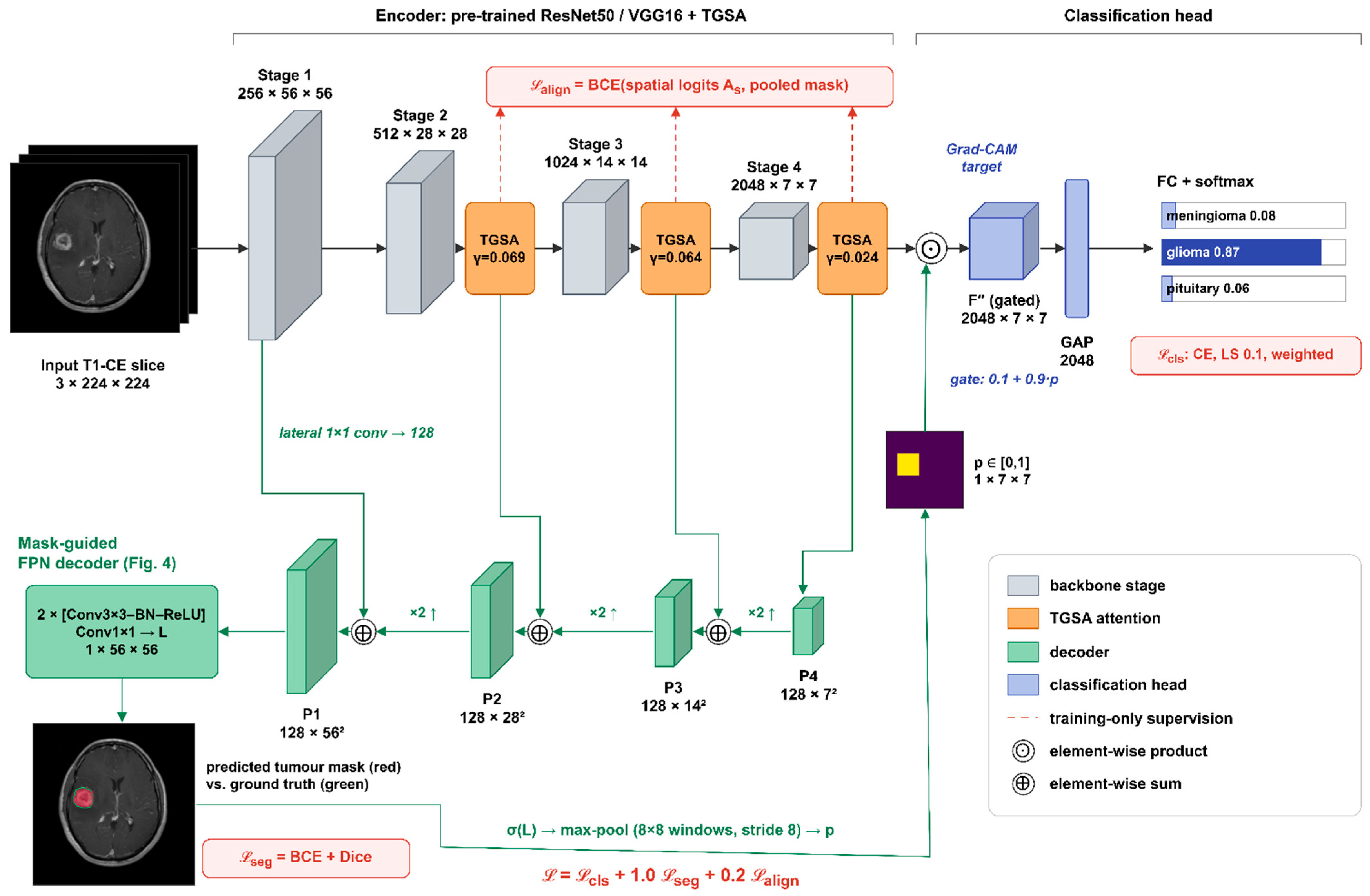
For ResNet50, the stage outputs are F1 ∈ R256×56×56, F2 ∈ R512×28×28, F3 ∈ R1024×14×14 and F4 ∈ R2048×7×7. For VGG16, these are the outputs of pooling layers 2–5, with 128, 256, 512, and 512 channels at the same resolutions.
2.6. Tumour-Guided Strip-Style Attention (TGSA)
Channel branch. The channel branch stacks three per-channel statistics, adding the standard deviation to the average and maximum of the Z-pool used by SSPANet:
Z = [ AvgH,W(X); MaxH,W(X); StdH,W(X) ] ∈ R3×C
Here odd(·) rounds up to the next odd integer, following the ECA-Net rule [15], and X′ = Mc ⊙ X.
Strip branch. X′ is reduced to m = max(16, C/16) channels by a 1 × 1 convolution with batch normalization and ReLU, giving U. Each row and each column of U is summarised by its average and maximum:
Sh = [AvgW(U); MaxW(U)] ∈ R2m×H, Sv = [AvgH(U); MaxH(U)] ∈ R2m×W
Grouped 1-D convolutions (kernel 7, m groups, followed by BN) model dependencies along each strip, and the results are broadcast back to H × W:
Astrip = expand(BN(GConv1D7(Sh))) + expand(BN(GConv1D7(Sv)))
Style branch. At each spatial position, the mean, standard deviation and maximum over channels, T = [μC(X′); σC(X′); maxC(X′)] ∈ R3×H×W, are mapped to m channels. The mapping uses a dilated 3 × 3 convolution (dilation 2) with BN and ReLU, followed by a 3 × 3 convolution with BN, and gives Astyle.
Fusion. The spatial logits and the module output are
where Ms ∈ [0, 1]1×H×W is the spatial attention map and γ is a learnable scalar initialized to zero. The zero initialization makes TGSA an identity mapping at the start of training, so it can be inserted at several stages of a pre-trained backbone. The logits As are supervised with the tumour mask (Section 2.9).
As = Conv1×1(ReLU(Astrip + Astyle)) ∈ R1×H×W
Ms = σ(As), TGSA(X) = X + γ ⋅ Ms ⊙ (Mc ⊙ X)
The learned gates remain small (γ = 0.008–0.131 across stages and P2 folds; 0.069, 0.064 and 0.024 for stages 2–4 of the fold-1 ResNet50 model shown in Figure 2 and Figure 3), so TGSA acts as a mild refinement of the pre-trained features. Figure 3b shows the learned spatial attention on held-out test slices of P2 fold 1.
2.7. Mask-Guided Feature-Pyramid Decoder
We use a light top-down decoder in the style of FPN [36] (Figure 4a), lighter than a full U-Net decoder [37]. It projects F1, , and (primes denote TGSA outputs) to 128 channels with 1 × 1 convolutions. Coarser maps are upsampled bilinearly and added to finer ones. The result passes through two 3 × 3 convolution–BN–ReLU blocks and a 1 × 1 convolution, which gives mask logits L at stride 4 (56 × 56). We then upsample these to 224 × 224 for the segmentation loss. The decoder adds 0.78 M parameters and uses tumour masks not used in [21] (gap G1).
2.8. Tumour-Focused Pooling (TFP) Gate
With a GAP head, evidence from anywhere in the slice, including skull, background or patient-specific anatomy, can drive the decision. The TFP gate converts the decoder output into a tumour probability for each cell of the 7 × 7 feature grid:
where Ωij is the (i,j)-th non-overlapping 8 × 8 window of the 56 × 56 map (kernel 8, stride 8). The gate then weights the final features before pooling:
with floor ϕ = 0.1. Two details matter. First, probabilities are pooled, not logits: averaging logits lets the strongly negative background logits of a cell only partly covered by tumour dominate, so small tumours were suppressed in an early design. Second, the head is linear in F″. Grad-CAM computed on F″ is therefore, up to ReLU and min–max normalization, the network’s class-activation map . This exactness does not extend to Grad-CAM++ or EigenGrad-CAM.
Stage-4 features have a receptive field that covers most of the slice. A gated cell can therefore still encode context from outside the tumour. For the same reason, a tumour-centred CAM on F″ is partly guaranteed by construction and does not by itself show that the decision relies on the lesion. We therefore test faithfulness directly with perturbations (Section 2.11). Figure 4b illustrates the mechanism on two test slices.
2.9. Training Objective
The total loss is
where M is the tumour mask, S is the set of TGSA stages, Lcls is the label-smoothed, class-weighted cross-entropy, and LDice is the soft Dice loss [38]. The attention-alignment term uses the area-averaged mask at each TGSA resolution as a soft target.
2.10. Hyper-Parameter Selection and Development History
The loss weights (λseg = 1.0, λatt = 0.2), the strip kernel size (7), the reduction width m, the decoder width (128) and all optimizer settings were fixed a priori to common default values and were not tuned.
We iterated on the classification head design in P1. We tried:
- a head that concatenated a tumour-pooled descriptor with a GAP descriptor;
- a multiplicative gate built from average-pooled logits;
- the final probability-pooled gate with floor ϕ = 0.1.
We evaluated these iterations on the seed-0 P1 test split, which is leaky and was also seen during development. For this reason, we report P1 results as non-held-out.
To remove this design leakage from the generalization claims:
- all P2 experiments were run after the design was frozen;
- the floor ϕ was additionally re-selected on P2 using validation data only. Within each fold, the ϕ ∈ {0.1, 0.3, 0.5} with the highest validation accuracy was chosen, and its test accuracy reported (Section 3.2).
2.11. Explanations, Localization Metrics and Faithfulness Tests
CAMs. For each model, we computed Grad-CAM [18], Grad-CAM++ [19], and EigenGrad-CAM [20] for the predicted class on the unflipped test image only. The target layer was the attention-refined last feature map for baselines and F″ for TG-SSPANet. We bilinearly upsampled maps to 224 × 224 and min–max normalized them.
Localization metrics. Against the expert mask M, we computed three metrics. The pointing game [39] is the fraction of slices whose map maximum lies inside the mask, dilated by 7 pixels. At the 224-pixel working resolution, this corresponds to about 16 pixels (7.7 mm) of the original 512-pixel image, close to the 15-pixel tolerance of [39]; we also report the pointing game without tolerance. Energy-in-mask [40] is Σ(CAM·M)/ΣCAM. CAM-IoU is the intersection-over-union of {CAM ≥ 0.5} with the mask. Results are given per fold of P2 (mean ± s.d.), per class and per tumour-size tercile.
Three reference explanations calibrate these numbers. The first is a centre prior (an isotropic Gaussian centred on the slice, σ = 0.25 of the image width), because pituitary tumours are central. The second is a uniform random map. The third, for decoder models, is the predicted tumour mask itself used as the explanation, which quantifies how much of a model’s localization is inherited from its segmentation branch.
Faithfulness. Two perturbation tests measure whether the classifier’s decision depends on the lesion.
Occlusion with controls. All occlusions are applied at the 256-pixel working scale (1 px ≈ 0.98 mm), using Euclidean distance to the expert mask (examples in Supplementary Figure S1). We report accuracy and the mean true-class probability without TTA under four conditions. In the tumour-removed condition, the tumour and a 6-px margin are inpainted using the fast-marching method of Telea [41]. In the sham removed condition, a region of identical shape and size is inpainted elsewhere in the head. It is the left–right mirror image of the tumour region or, if that overlaps the tumour, a translated copy that must lie at least 80% inside the head. This condition tests whether the inpainting perturbation by itself degrades or biases predictions. In the tumour + decoys removed condition, the tumour region and two additional similarly shaped regions elsewhere in the head are inpainted, so the inpainted footprint no longer uniquely marks the tumour’s location. In the graded context condition, the tumour plus all tissue within 0 (tumour only), 6, 15, 30, or 60 px is kept, and the rest is set to zero. We regard the 15-px ring as the perilesional condition; at 60 px much of the hemisphere is included. All conditions are evaluated on the same matched subset of slices for which both a valid sham region and two valid decoy regions exist (2740 of 3064 slices, 89%), so that the tumour-removed, sham and decoy accuracies are directly comparable. For TG-SSPANet, we also recorded what the decoder predicts on the occluded slices: whether any cell of the 7 × 7 gate input p reaches 0.5 (otherwise the gate is close to uniform and the model pools the whole slice) and where the predicted mask lies.
Positive controls. The two-stage ROI-crop classifier, trained only on tumour-centred crops, and the oracle ground-truth-gated model are evaluated under the same conditions. For the ROI-crop classifier, we apply the occlusion to the full slice and then crop the result. The crop box comes either from the mask the TG-SSPANet decoder predicts on the original, unoccluded slice (as in the two-stage pipeline) or from the ground-truth mask. In both variants, the crop is independent of the occlusion.
Location-only controls. To measure how much class information is carried by the tumour’s position, size, and shape alone, we trained two classifiers on the same P2 folds. The first is a ResNet50 trained with the proposed recipe on the binary expert mask as its only input. The second is a gradient-boosting classifier on nine mask-geometry features (centroid, distance from the midline, area, bounding-box height and width, extent, eccentricity and orientation).
Tile-shuffle control. To remove location and anatomical layout while keeping local tissue statistics, we cut the head region into 16 × 16-pixel tiles (about 16 mm) and randomly permuted all tiles that lie entirely inside the head. Three versions were evaluated on the matched subset. In context shuffled, the tumour with its 6-px margin stays in place and only the tiles that do not touch it are permuted. In removed + shuffled, the tumour is first inpainted as above and all head tiles, including the inpainted ones, are then permuted, so that neither the tumour, nor its footprint, nor the surrounding anatomy stays where it was. In all shuffled, the tiles of the original slice are permuted, which scatters pieces of the tumour as well. Shuffling preserves the intensity and texture statistics of the tissue and the outline of the head, whose partially covered border tiles are not moved. The tile edges are themselves unusual, so the context-shuffled condition, which keeps the lesion intact, indicates the cost of this artefact.
Deletion and insertion [29]. Pixels are ranked by the model’s Grad-CAM++ map and progressively replaced by a heavily blurred copy of the slice (Gaussian, σ = 10 px), in 11 steps from 0% to 100% of pixels. This gives a deletion curve of the true-class probability. The reverse process, inserting original pixels into the blurred slice, gives an insertion curve. We report the area under each curve (AUC), together with the same quantities for a random pixel order. Lower deletion AUC and higher insertion AUC indicate a more faithful ordering. Under a random order, deleting a fraction f of the pixels produces the same kind of image as inserting a fraction 1 − f, so the random-order deletion and insertion curves are mirror images and have identical AUCs.
2.12. Mask-Using Baselines and Ablations on P2
Because the annotations are central to our argument, we compared TG-SSPANet on P2 against the simplest ways to exploit them. All of these baselines use the proposed recipe:
- Two-stage ROI-crop classifier. A tumour box with a 25% margin (at least 64 pixels at the 256-pixel scale) is cropped, resized and classified by a ResNet50. Training uses crops from the ground-truth masks. At test time, the crop comes from the mask that the TG-SSPANet decoder of the same fold predicts, giving a realistic segment-then-classify pipeline. We also report the oracle variant, which crops with the ground-truth mask at test time.
- Oracle ground-truth gate. TG-SSPANet with p computed from the ground-truth mask in training and testing. This is an upper bound for TFP.
- Y-Net-style joint learning [30]. TG-SSPANet without the TFP gate: the segmentation decoder and attention supervision are trained jointly with the classifier, but the classifier pools the whole slice. This model also serves as the explanation-supervision baseline; we did not evaluate an input-gradient penalty [42].
The P2 ablation compares the same-recipe ResNet50, the Y-Net-style model (no TFP), and TG-SSPANet with ϕ ∈ {0.1,0.3,0.5}. On P2, we trained all seven attention modules (Coordinate, GCNet, SPNet, SRMNet, SE, CBAM, and SSPANet) with ResNet50 under the proposed recipe, and we trained the VGG16 backbone with and without SSPANet under both recipes. To separate the individual components, we also trained, on the same folds and with the same recipe, TGSA alone with and without the alignment loss, the decoder alone (joint segmentation without TGSA or TFP), the decoder with TFP but without TGSA, and the full model without the alignment loss. The ablation of the individual TGSA branches (channel, strip and style) was run only on P1 with a single seed (Supplementary Figure S2).
2.13. Statistics, Calibration and Cost
Reported metrics. We report accuracy, weighted precision, recall and F1 (the weighted averages reproduce the equal values reported in [21]), macro-F1, Cohen’s κ, the Matthews correlation coefficient (MCC) and the macro one-vs-rest AUC.
P1 statistics. We trained each configuration with three seeds. Paired t-tests across seeds and exact McNemar tests [43] on the seed-0 predictions are reported descriptively, with Holm correction [44] within each backbone. On a fixed test set these tests reflect optimization noise rather than generalization.
P2 statistics.
- Slice-level accuracy is reported as the mean ± s.d. over folds. We obtain a 95% confidence interval from a patient-clustered bootstrap (2000 resamples of the 233 patients) over the pooled out-of-fold predictions, because slices from the same patient are not independent.
- We compute patient-level accuracy, the clinically relevant unit, by averaging the class probabilities across all slices of a patient, with a bootstrap CI over patients. Because this number depends on the aggregation rule, we also report a majority vote over the slice predictions (ties broken by the mean probability), the prediction of the single most confident slice, and a strict rule under which a patient counts as correct only if every slice is correct, together with the number of patients whose slices are assigned to different classes.
- Comparisons with TG-SSPANet use the corrected resampled t-test of Nadeau and Bengio [45], which accounts for the overlap of training sets across folds. None of these comparisons was specified before the results were known, so all p-values in this paper are descriptive: they express the size of a difference relative to the fold-to-fold variation and do not test pre-stated hypotheses. Table 2 lists each p-value after Holm correction [44] over the comparisons with the two reference models of each backbone (the plain backbone and the backbone with SSPANet, i.e., the backbone and the method under reproduction) and over all comparisons of that backbone.
Table 2.
P2 (patient-wise five-fold cross-validation): slice-level accuracy (mean ± s.d. over folds; 95% CI from a patient-clustered bootstrap of the pooled out-of-fold predictions), patient-level accuracy with 95% bootstrap CI, Cohen’s κ and comparison with TG-SSPANet of the same backbone (Nadeau–Bengio corrected resampled t-test). All p-values are descriptive, because no comparison was specified in advance. p (ref.): Holm-adjusted over the comparisons with the two reference models of each backbone (plain backbone and backbone + SSPANet); p (all): Holm-adjusted over all comparisons of that backbone. Orig.: original recipe of [21]; all other models use the proposed recipe.
Calibration. We summarise calibration by the expected calibration error (ECE, 15 bins) [46] and the Brier score, and illustrate it with reliability diagrams. We summarise selective-prediction performance by the area under the risk–coverage curve (AURC) and accuracy at 90% coverage [47]. We also applied temperature scaling [48]: we fitted a single temperature per fold by minimizing the negative log-likelihood on that fold’s validation patients, then applied it to the test predictions. The temperature acts on the flip-averaged probabilities that constitute the model’s prediction (the logarithm of the averaged probabilities is divided by T and renormalized with a softmax), so slice-level predictions are unchanged. We recomputed the ECE, AURC, accuracy at 90% coverage, and patient-level accuracy (which averages probabilities over a patient’s slices and can therefore change) on the pooled test folds.
Cost and hardware. We report the number of parameters and GMACs (multiply–accumulates for one 224 × 224 image). We measured latency after 3 warm-up iterations as the mean of 10 forward passes on a batch of 32 images, in FP16 autocast with CUDA synchronization, on a single NVIDIA GeForce RTX 3060 (12 GB) with PyTorch 2.5.1 [49], CUDA 12.1, and Python 3.12.
Simulated acquisition shifts. We had no independent annotated test set (Section 4.5), so we could not test other hospitals or scanners directly. As a partial check, we evaluated the P2 models on their test folds after simulated acquisition changes, without retraining and without TTA: additive Gaussian noise with a standard deviation of 2% and 5% of the intensity range, a smooth multiplicative bias field of ±20% and ±40%, gamma contrast changes (γ = 0.7 and 1.5), halved in-plane resolution, and a combination of a ±20% bias field, γ = 1.2, halved resolution and 2% noise. For the two-stage ROI-crop pipeline, the crop came from the decoder’s prediction on the perturbed slice. These perturbations mimic some differences between scanners, but not changes in sequence, field strength or patient population, and they do not replace external validation.
Determinism. Training of TG-SSPANet is not bit-wise deterministic, because the GPU backward passes of bilinear upsampling (in the decoder) and of max pooling (in the gate) accumulate gradients with atomic additions, whose order varies between runs. To quantify the effect, we trained TG-SSPANet four times and the plain ResNet50 three times on P1 with an identical seed and configuration, using the proposed recipe (Section 3.1).
3. Results
3.1. Reproduction of the Original Study (P1, Non-Held-Out)
Table 1 and Figure 5 compare the values reported in [21] with our reproduction under the original recipe (mean ± s.d. over three seeds).
Figure 5.
P1 reproduction (image-level, patient-leaky, non-held-out). Open diamonds: accuracy reported in [21]; filled circles: our reproduction under the original recipe (mean ± s.d. over three seeds); red: TG-SSPANet with the proposed recipe, for reference. Every reproduced configuration exceeds 98%.
Reproduced baselines exceed the reported values. The differences range from 1.5 points (ResNet50 + SSPANet: 98.48% versus 97%) to 43.9 points (VGG16 + GCNet: 98.91% versus 55%; the reported κ = 0.00 is consistent with a degenerate run). Every configuration exceeds 98% on P1.
Possible sources of the gap. Several details that affect performance are not reported in [21]: input size, ImageNet pre-training, the classification head, where the attention module is inserted, and the exact split. The dataset is also widely redistributed as JPEG conversions, for example in Kaggle mirrors [50], which differ in intensity scaling and resolution and are sometimes merged with other sources. We therefore cannot identify the cause of the gap. We note only that standard fine-tuning of pre-trained backbones saturates P1.
No P1 superiority claim. TG-SSPANet trained with the proposed recipe reached 99.67 ± 0.33% (ResNet50) and 99.24 ± 0.50% (VGG16). It misclassified one, zero and two of 307 slices at seeds 0, 1 and 2, respectively. However, P1 is patient-leaky and was used during development (Section 2.10), and a plain ResNet50 trained with the proposed recipe also reached 100% at seed 0. We therefore make no superiority claim on P1: differences between the strongest configurations amount to one or two test images, and no comparison remained significant after Holm correction (smallest adjusted p = 0.46; Supplementary Table S1). P1 confusion matrices, ROC curves and the quantitative localization of all P1 models are given in Supplementary Figures S3–S5.
Determinism. The full TG-SSPANet run of the P1 ablation (Supplementary Figure S2; 100% accuracy, Grad-CAM++ pointing game 0.844) and the main seed-0 model (one error, pointing game 0.827) were separate training runs with the same configuration. They differ because GPU training is not bit-wise deterministic (Section 2.13). Across the four repeated TG-SSPANet runs, the number of errors on the 307 test slices was 0–4 (98.7–100% accuracy), and any two runs disagreed on 1–4 predictions. The three plain ResNet50 runs, which contain neither layer, were bit-identical. On P1, the run-to-run variation of TG-SSPANet is therefore as large as the differences between the strongest configurations.
Figure 6 and Figure 7 show the training curves of six P1 configurations. TG-SSPANet converges more slowly in the first epochs because of its zero-initialized gates and learning-rate warm-up. The original-recipe baselines stop early on validation loss after 13–21 epochs on average.
Figure 6.
Training and validation accuracy and loss with the ResNet50 backbone (P1, seed 0) for the baseline, Coordinate attention, GCNet, SPNet, SRMNet and TG-SSPANet. Baselines use the original recipe of [21] and stop early on validation loss. The training loss of TG-SSPANet includes label smoothing and the segmentation and alignment terms and is not comparable in absolute value.
Figure 7.
Training and validation accuracy and loss with the VGG16 backbone (P1, seed 0) for the same six models as Figure 6.
3.2. Leakage-Free Classification Performance (P2)
Figure 8.
P2 slice-level accuracy of every model. Dots: individual folds; shaded bar: 95% CI from a patient-clustered bootstrap of the pooled out-of-fold predictions; black tick: pooled accuracy. The text on the right gives the fold mean ± s.d. and the patient-level accuracy. Grey: original recipe of [21]; blue: proposed recipe; green: mask-using models and ablations; red: TG-SSPANet.
Effect of removing leakage. Accuracy falls substantially for every model. Under the original recipe, the drop is 5.4 points for ResNet50 (98.59% → 93.21%), 6.5 for ResNet50 + SSPANet (98.48% → 91.97%), 8.7 for VGG16 (98.70% → 90.03%) and 7.1 for VGG16 + SSPANet (99.24% → 92.10%). For TG-SSPANet, the drop is 2.9 points (ResNet50) and 2.6 points (VGG16).
Effect of the training recipe. The proposed recipe alone raises P2 accuracy by 2.4–4.7 points across the four original-recipe configurations (e.g., ResNet50: 93.21% → 95.61%; VGG16: 90.03% → 94.73%). This is more than any attention module adds under a fixed recipe: under the proposed recipe, all seven attention modules with ResNet50 (Coordinate, GCNet, SPNet, SRMNet, SE, CBAM and SSPANet) reach 95.06–96.24%, between −0.55 and +0.63 points from the plain backbone (95.61%), and the differences were small. For six of the seven modules there was no detectable difference: the 95% confidence intervals of the paired fold differences included zero (Supplementary Table S7). SPNet was 0.36 points higher in all five folds (95% CI 0.03 to 0.68), but this did not hold after correction for the seven comparisons (Holm-adjusted p = 0.27), and a gain of this size is of no practical importance.
TG-SSPANet versus same-recipe controls. With ResNet50, TG-SSPANet obtained 96.82 ± 0.95% slice-level accuracy (pooled 95% CI 95.1–98.2%, patient-clustered bootstrap), 98.28% patient-level accuracy (95% CI 96.6–99.6%) and κ = 0.950. This is numerically the highest slice-level accuracy of all ResNet50 models. However, its confidence interval overlaps those of the same-recipe controls (plain ResNet50 93.4–97.3%; ResNet50 + SSPANet 94.0–97.3%), and the descriptive corrected resampled t-tests gave a Holm-adjusted p = 0.725 against both reference models. The paired differences were +1.20 points (95% CI −2.05 to +4.46) and +0.99 points (95% CI −2.15 to +4.14), respectively. The strongest same-recipe attention model, ResNet50 + SRMNet (96.24%), (CI 94.4–97.7%) is 0.58 points below TG-SSPANet (better on 4 of 5 folds; unadjusted p = 0.573, Holm-adjusted p = 1.00; paired difference +0.57 points, 95% CI −2.02 to +3.16). Several mask-using variants perform equally well: the Y-Net-style model without TFP (96.36%), the ground-truth-gated oracle (96.80%), and the two-stage ROI-crop classifier with predicted masks (95.86%). The ROI-crop classifier reaches the highest patient-level accuracy (98.71%, CI 97.0–100%).
With VGG16, TG-SSPANet (96.64 ± 1.52%, patient level 97.85%) outperformed both same-recipe controls on all five folds (VGG16: 94.73%; VGG16 + SSPANet: 95.48%). The descriptive p-values against the two reference models were 0.199 and 0.064, and only the original-recipe VGG16 had an adjusted p below 0.05 (0.017).
Location-only control. The ResNet50 trained on the binary tumour mask alone, without any image content, reached 70.80 ± 2.66% slice-level and 79.0% patient-level accuracy, far above the 46.5% of always predicting the majority class (glioma). A gradient-boosting classifier on nine mask-geometry features reached 69.2 ± 1.4%. Tumour position, size and shape therefore carry substantial class information on this dataset (Section 3.5).
Validation-only choice of φ. When the gate floor φ ∈ {0.1, 0.3, 0.5} was chosen on validation data only within each fold, the selected value varied between folds and the test accuracy was 96.66 ± 1.45%. This is indistinguishable from the fixed φ = 0.1.
3.3. Explanations: Qualitative Comparison
Figure 9 follows the layout of Figure 8 and Figure 9 in [21] for six ResNet50 models trained with the same recipe: the no-attention baseline, four attention modules evaluated in [21] (Coordinate, GCNet, SPNet, and SRMNet), and TG-SSPANet. We use held-out patients from the first patient-wise fold, so the qualitative and quantitative explanation results follow the same protocol; the corresponding P1 grids from the original study layout, including VGG16, are shown in Supplementary Figures S6 and S7.
Figure 9.
Qualitative explanation comparison on held-out patients (P2 fold 1) for six ResNet50 models trained with the same recipe: the baseline, Coordinate attention, GCNet, SPNet, SRMNet and TG-SSPANet (red frame). Columns: tumour type × CAM method. Green: ground-truth tumour contour.
For the superficial meningioma, all models place the maximum of their maps on the tumour. For the glioma and the pituitary tumour, the baseline maps are broad and centred on the midline, the ventricles or the posterior fossa. In contrast, TG-SSPANet produces compact maps centred on the tumour. Quantitative results over all held-out slices follow.
3.4. Localization of Explanations Against the Expert Masks (P2)
Table 3.
P2 localization of Grad-CAM++ explanations against the expert tumour masks (mean over the five test folds; pointing game ± s.d. over folds). PG: pointing game with 7-pixel tolerance; PG0: without tolerance; EiM: energy in mask; IoU: CAM-IoU at 0.5; per-class and per-size-tercile (small, medium, large) values are pointing games. Reference rows use no model. Orig.: original recipe.
Figure 10.
P2 localization of Grad-CAM++ explanations (mean ± s.d. over folds): pointing game (left) and energy in mask (right). Dashed line: centre prior; dotted line: random map; dash-dotted line: the TG-SSPANet decoder mask used directly as the explanation. Colours as in Figure 8.
Baselines are near the centre prior. For every ResNet50 baseline, including the same-recipe controls, the pointing game was 0.16–0.30. This is close to or below the centre prior (0.27) and well above a random map (0.04). For pituitary tumours, which lie near the image centre, the centre prior scores 0.39, above every baseline (≤0.17) and far below TG-SSPANet (0.754). The original-recipe models scored 0.22.
TG-SSPANet localizes far better. It reached 0.811 ± 0.025, and the ground-truth-gated oracle reached 0.823. The improvement held:
- without the 7-pixel tolerance (0.554 versus 0.09–0.18 for the baselines);
- for Grad-CAM (0.807) and EigenGrad-CAM (0.794);
- for all tumour types, including the centrally located pituitary tumours (0.754 versus ≤0.17);
- for all tumour sizes, including the smallest tercile (0.618 versus ≤0.12).
With VGG16 the pattern was the same: 0.729 for TG-SSPANet versus 0.27–0.31 for the baselines.
Energy inside the tumour. Energy-in-mask rose from 0.06–0.09 to 0.225. Even for TG-SSPANet, about 78% of the CAM energy therefore lies outside the tumour mask, reflecting the coarse 7 × 7 resolution of the explained feature map.
The gate is the decisive component. Without the TFP gate (Y-Net-style model), localization fell to 0.259, the baseline level, even though that model’s decoder segments the tumour just as well. Raising the gate floor lowered localization monotonically (φ = 0.3: 0.682; φ = 0.5: 0.559).
Much of the localization is inherited from the decoder. Used directly as an explanation, the decoder’s own mask hits the tumour in 0.948 of slices, with energy-in-mask 0.799, more than TG-SSPANet’s Grad-CAM++ achieves. The localization of TG-SSPANet’s CAM is thus largely a consequence of its segmentation branch, as the construction of Equation (8) implies. Whether the classifier’s decision relies on the lesion is a separate question, examined next.
3.5. Faithfulness: Does the Decision Depend on the Lesion? (P2)
Table 4 and Figure 11 report the occlusion tests with controls on the matched subset, Supplementary Table S2 gives every condition and context ring for every model, and Figure 12 shows the deletion and insertion curves.
Table 4.
P2 occlusion with controls on the matched subset (2740 slices with a valid sham and two valid decoy regions; accuracy, mean over the five test folds; single forward pass without TTA) and deletion/insertion AUCs for Grad-CAM++ pixel ordering (random ordering in brackets). Orig.: original slice; Sham: a same-shaped region elsewhere in the head is inpainted; Rem.: tumour removed (inpainted); Decoy: tumour and two same-shaped decoy regions inpainted; Only: tumour only; +15/+60: tumour plus 15 or 60 px of surrounding tissue (1 px ≈ 0.98 mm). All rings and standard deviations are given in Supplementary Table S2.
Figure 11.
P2 occlusion with controls on the matched subset. (a) Accuracy on the original slices, with a same-shaped region inpainted elsewhere (sham), with the tumour inpainted, with the tumour and two same-shaped decoys inpainted, and with only the tumour kept (mean ± s.d. over folds; dotted line: chance). (b) Accuracy as a function of the tissue kept around the tumour (0–60 px, then the full slice); the x-axis positions are categorical and not to scale, and all tissue outside the ring is set to zero, which makes these images out of distribution. The ROI-crop classifier (purple) and the oracle ground-truth gate (orange) are positive controls.
Figure 12.
P2 deletion (a) and insertion (b) curves of the true-class probability for Grad-CAM++ pixel ordering (mean over folds); dotted red: TG-SSPANet with random ordering.
Tumour removed. When the tumour and a 6-px margin were inpainted, the whole-slice models still classified 80–86% of the slices correctly, far above chance (33%) and the majority-class rate (46.5%). TG-SSPANet lost slightly more accuracy (96.6% → 81.3%) than the same-recipe controls (94.4–96.2% → 82.0–84.0%), within the fold-to-fold s.d. (3–6 points).
Three controls constrain the interpretation.
- The inpainting perturbation does not by itself degrade or bias predictions: inpainting a same-shaped region elsewhere in the head (sham) changed accuracy by at most 0.4 points for every model.
- The uniqueness of the inpainted footprint explains only a few points. When two decoy regions of the same shape and size were inpainted in addition to the tumour, every inpainted region still showed the tumour’s shape and size, but the footprint no longer singled out the tumour’s location. Accuracy fell by a further 1.2–3.6 points for the whole-slice models (TG-SSPANet 81.3% → 77.7%; ResNet50 83.3% → 80.8%) and remained far above chance.
- Tumour position and shape carry substantial information (location-only classifier: 70.8%; Section 3.2). The decoys remove only the uniqueness of the location: shape and size remain visible in each inpainted region, and location can still be inferred from the surrounding anatomy. The remaining 78–84% can therefore come from tissue outside the lesion, which encodes location (for example, sellar anatomy or proximity to the dura) and mass effect, and from lesion geometry that remains visible after inpainting; our controls cannot apportion it between these sources.
The graded-context results must be read with caution, because setting all tissue outside the ring to zero produces images unlike any training slice. With the tumour plus 15 px (≈15 mm) of surrounding tissue, the whole-slice models trained with the proposed recipe reached only 31–41% (original-recipe ResNet50 models 46–54%), whereas the lesion-centred ROI-crop positive control reached 67.5% under the same condition. The low whole-slice accuracies with narrow rings therefore reflect this distribution shift at least as much as missing information, and they do not show that perilesional tissue is uninformative. With 60 px, which includes much of the hemisphere, the whole-slice models reached 86–94% (original-recipe models 61–71%). Our tests therefore cannot separate information the models read from the lesion’s location and shape from information in the surrounding tissue, nor can they localize it within the slice. They show that the retained information is not an inpainting artefact.
Tile-shuffle control. Table 5 separates spatial layout from tissue statistics. When only the surroundings of an intact tumour were shuffled, the whole-slice models kept 84–93% accuracy and the lesion-only ROI-crop control 94.6%. Among the whole-slice models, the two gated models lost the least (TG-SSPANet 96.6% → 90.1%; oracle gate 96.5% → 93.2%; same-recipe GAP models 95.2–96.2% → 83.8–87.4%), so pooling over the predicted tumour makes the decision somewhat more dependent on the lesion itself, although the differences are within the fold-to-fold variation. When the tumour was removed and all head tiles were shuffled, so that neither the tumour, its footprint nor the anatomical layout stayed in place, accuracy fell from 80–85% (tumour removed only) to 60–74%. Location and anatomical layout therefore account for between 8 and 24 points of the accuracy that survives tumour removal. These are upper bounds, because shuffling already cost 1–12 points when the tumour was left intact, and part of that cost is due to the tile edges rather than to lost information. The remainder, still well above chance and the majority-class rate, must come from what shuffling preserves: the intensity and texture statistics of the tissue and the unshuffled outline of the head, which reveals the imaging plane and the level of the slice. Shuffling the original slice, which also scatters the tumour, gave similar values (59–76%), so the texture of the lesion without its spatial integrity adds little.
Table 5.
Tile-shuffle control on the matched subset (2740 slices; accuracy, mean ± s.d. over the five P2 test folds; single forward pass without TTA). Head tissue was cut into 16 × 16-pixel tiles that were randomly permuted. Context shuffled: tumour and 6-px margin kept in place, all other head tiles permuted; Removed + shuffled: tumour inpainted, then all head tiles permuted; All shuffled: all head tiles of the original slice permuted. Tumour removed is repeated from Table 4 for comparison. Orig.: original recipe.
Decoder output after tumour removal. Because the gate depends on the decoder, a decoder that finds no tumour after inpainting would turn TG-SSPANet into a whole-slice classifier. This happened only in a minority of slices (Supplementary Table S6). On the original slices, the decoder of the ResNet50 TG-SSPANet opened at least one gated cell in 99.7% of slices. After the tumour was inpainted, it still did so in 88.6%, and 56% of its predicted mask lay inside the inpainted region, which the decoder evidently still recognised as abnormal. In the remaining 11.4% of slices the gate was close to uniform, and accuracy there (82.1%) was similar to that with an open gate (81.1%). With decoys, the gate opened in 91.4% of slices, and the predicted mask fell partly in the former tumour region (43%) and partly in the decoys (17%). The VGG16 model behaved similarly but fell back to a uniform gate more often (28.2% after tumour removal). The accuracy that TG-SSPANet retains after inpainting is therefore not explained by a fallback to whole-slice pooling; in most slices, the model still pooled evidence around the former tumour site.
Positive controls. The two-stage ROI-crop classifier, trained only on tumour-centred crops, is a model known to rely on the lesion. It lost the most accuracy when the tumour was removed (95.6% → 64.8%) and reached 67.5% with 15 px of context and 93.5% with 30 px. The result was the same whether the crop box came from the predicted mask on the unoccluded slice or from the ground-truth mask (64.8% versus 64.2%), so a failed crop does not cause the drop. The oracle ground-truth gate behaved like TG-SSPANet.
Tumour only. Tumour-only accuracy was low for all models, including the positive control (25–46%). Several models scored below chance. Supplementary Table S3 shows why: on zero-background images, the same-recipe models and the TG-SSPANet variants predicted meningioma for most slices, and the original-recipe ResNet50 favoured glioma. Because meningioma makes up only about a quarter of the matched slices, this systematic bias yields accuracies below 33%. The tumour-only condition is therefore strongly out of distribution and should be read as a lower bound on what the lesion alone supports, not as evidence that the models ignore it.
Deletion and insertion. Ranking pixels by TG-SSPANet’s Grad-CAM++ removed the evidence faster than random ordering (deletion AUC 0.504 versus 0.584). The map therefore identifies pixels that the classifier uses. The deletion AUC was similar to that of the best same-recipe controls (0.508–0.531), and insertion AUCs were indistinguishable across the ResNet50 models (0.81–0.84). The same held for VGG16. As explained in Section 2.11, random-order deletion and insertion AUCs are identical by symmetry.
3.6. Mask-Using Baselines and Ablation (P2)
Figure 13 summarises the P2 ablation.
Figure 13.
P2 ablation and mask-using baselines: (a) slice-level accuracy and (b) Grad-CAM++ pointing game (mean ± s.d. over folds). The ROI-crop classifiers are not shown in (b) because their CAMs refer to the crop rather than the slice.
Accuracy. All mask-using variants reach 95.9–96.8% accuracy (paired differences from TG-SSPANet with 95% confidence intervals in Supplementary Table S7), and none differs from TG-SSPANet by more than the fold-to-fold variation. These include:
- the segmentation decoder and attention supervision without the gate (Y-Net-style);
- TG-SSPANet with φ ∈ {0.1, 0.3, 0.5};
- the ground-truth-gated oracle;
- the two-stage ROI-crop classifier.
Localization. In contrast, localization separates the variants sharply (Section 3.4): only the gate places the classifier’s evidence on the tumour, and its effect decreases monotonically as φ increases. The oracle gate improves localization only slightly over the predicted gate (0.823 versus 0.811). This is consistent with the decoder’s high tumour detection rate on held-out patients (Dice 0.80; pointing game mask score 0.948).
Where TFP stands relative to the simplest pipeline. TFP is therefore not more accurate than “segment the tumour, then classify the crop”. Its contribution is to make the attribution of a single end-to-end classifier coincide with the lesion, at a cost of 1.34 M parameters and 1.2 GMACs (Table 1).
Component ablation. Table 6 separates the four components on the P2 folds. Accuracy varied little: all eight variants lay between 95.2% and 96.8%, within the fold-to-fold standard deviations (0.7–1.9 points), and no single component raised accuracy consistently. Adding TGSA to the plain backbone changed accuracy by +0.3 points without the alignment loss and by −0.4 points with it; adding the decoder alone changed it by +0.3 points; and adding TGSA to a model that already had the decoder and TFP changed it by +0.4 points. Localisation, by contrast, depended on a single component. Every variant with TFP reached a Grad-CAM++ pointing game of 0.80–0.81, and every variant without it stayed at the baseline level (0.25–0.33), whether or not TGSA, the alignment loss or the decoder was present. The decoder segmented the tumour equally well with or without TGSA (Dice 0.79–0.80). The benefit of TG-SSPANet’s explanations therefore comes from the combination of decoder and TFP, and TGSA can be removed without a measurable loss in accuracy or localisation.
Table 6.
P2 component ablation of TG-SSPANet (ResNet50, proposed recipe, five patient-wise folds; ✔: component present). TGSA: attention modules after stages 2–4; Align. loss: supervision of the TGSA logits with the mask; Decoder: mask-guided FPN decoder with segmentation loss; TFP: tumour-focused pooling gate (φ = 0.1). Slice acc.: mean ± s.d. over folds; Patient acc.: class probabilities averaged over each patient’s slices; PG: Grad-CAM++ pointing game with 7-pixel tolerance (mean ± s.d. over folds); Dice: predicted versus expert mask. The first row is the same-recipe ResNet50, the fifth the Y-Net-style model and the last the full TG-SSPANet of Table 2.
3.7. Calibration and Selective Prediction (P2)
Table 7.
P2 calibration and selective prediction (pooled out-of-fold predictions). ECE: expected calibration error (15 bins), before and after temperature scaling fitted on each fold’s validation patients; AURC: area under the risk–coverage curve (lower is better); Acc@90%: accuracy on the 90% most confident slices. We did not apply temperature scaling to the ROI-crop classifier or the original-recipe SSPANet.
Figure 14.
P2 calibration of the ResNet50 models (pooled out-of-fold predictions, before temperature scaling): (a) reliability diagram (10 equal-width confidence bins; bins with fewer than 5 slices are omitted; the legend gives the 15-bin ECE of Table 7); (b) risk–coverage curves for selective prediction; (c) number of slices per confidence bin (log scale; numbers for TG-SSPANet). Most slices fall in the two highest bins, so low-confidence points rest on few slices.
Confidence. Label smoothing reduces overconfidence and can leave models under-confident [51], and the proposed-recipe models are under-confident. TG-SSPANet has a mean confidence of 0.896 at an accuracy of 0.968 and an ECE of 0.074, versus 0.062–0.067 for the same-recipe controls and 0.031 for the original-recipe ResNet50. At the same time, TG-SSPANet has the lowest Brier score of all ResNet50 models (0.064).
Selective prediction. Its selective-prediction performance is good. At 90% coverage, rejecting the 10% least confident slices, accuracy rises to 98.4%. Among all models, the two-stage ROI-crop classifier has the lowest area under the risk–coverage curve (AURC 0.0095, compared with 0.0158 for TG-SSPANet; Table 7). These selective-prediction results are computed from the unscaled, flip-averaged probabilities. Confidence could therefore help to identify uncertain cases for referral, although no referral threshold was fixed in this study (Section 4.4).
Temperature scaling. A single temperature fitted per fold on validation patients (T = 0.20–0.98 for TG-SSPANet, mean 0.66) sharpened underconfident probabilities. It reduced TG-SSPANet’s ECE from 0.074 to 0.019 and its Brier score from 0.064 to 0.058, while leaving slice-level predictions unchanged. The same-recipe controls improved similarly (ECE 0.019–0.025), and VGG16 TG-SSPANet improved from 0.110 to 0.022. Scaling, however, changes the ordering of confidences across slices and the patient-level averages (Supplementary Table S4). For TG-SSPANet, the AURC rose from 0.0158 to 0.0193, accuracy at 90% coverage changed from 98.4% to 98.2%, and patient-level accuracy changed from 98.3% to 98.7%. For the same-recipe controls, AURC also rose slightly (ResNet50: 0.028 → 0.036). Well-calibrated probabilities therefore come at a small cost in confidence ranking.
3.8. Predictions and Error Analysis (P2)
Figure 15 shows test predictions of TG-SSPANet on the first patient-wise fold. Figure 16 shows all 17 errors (of 542 slices) of that fold, with the Dice of the predicted mask and the patient identifier.
Figure 15.
Test predictions of TG-SSPANet on patient-wise fold 1 (held-out patients). Green: ground-truth tumour; red/yellow: predicted tumour mask; title: true class, predicted class and confidence.
Figure 16.
All misclassified slices of TG-SSPANet on patient-wise fold 1 (17 of 542), with the Dice of the predicted mask and the patient identifier. Errors cluster within patients, and the lesion is usually localized correctly.
Error types. Across all five folds, TG-SSPANet made 98 slice-level errors in 36 patients. The dominant confusions were:
- glioma predicted as meningioma (35 errors);
- meningioma predicted as pituitary tumour (30 errors);
- meningioma predicted as glioma (20 errors);
- pituitary tumour predicted as meningioma (9 errors).
Errors cluster within patients. Twenty of the 36 affected patients account for more than one error. Patient-level accuracy (98.3%) exceeds slice-level accuracy because averaging the probabilities across a patient’s slices lets the correctly classified majority outvote the minority of erroneous ones; clustering alone would not produce this gain.
Patient-level aggregation. The patient-level figure depends on how slices are combined (Table 8). For TG-SSPANet, a majority vote gave 98.7% (3 of 233 patients wrong) and averaging the probabilities 98.3% (4 wrong), so the result does not depend on probability averaging in particular. Taking only the most confident slice gave 96.1%. Under the strict rule that every slice must be correct, accuracy fell to 84.5%, within the range of the same-recipe whole-slice models (82.0–86.3%) and above the ROI-crop pipeline (79.8%). For a referral decision, averaging hides the disagreement between slices: 35 patients (15.0%) had slices assigned to more than one class, and they included three of the four patients misclassified by probability averaging. A practical rule would report the averaged prediction but refer every patient whose slices disagree; here, this would send 15% of patients for review and leave one misclassified patient unflagged. We keep probability averaging as the main patient-level result because it uses every slice and gives patient-level probabilities, but the strict and discordance figures show how much slice-level disagreement it conceals.
Table 8.
Patient-level accuracy of the P2 models under different aggregation rules (233 patients, pooled out-of-fold predictions; number of misclassified patients in brackets). Mean probability: class probabilities averaged over a patient’s slices (the rule used in Table 2); Majority vote: most frequent slice prediction, ties broken by the mean probability; Most confident slice: prediction of the slice with the highest confidence; All slices correct: a patient counts as correct only if every slice is correct; Discordant patients: patients whose slices are assigned to more than one class. Orig.: original recipe.
Lesion localization in the errors. On the misclassified slices, the predicted mask overlapped the annotated tumour in 93.9% of cases and reached Dice ≥ 0.5 in 85 of 98 (87%; median Dice 0.88, interquartile range 0.69–0.94). Most errors are therefore misinterpretations of a correctly localized lesion: parasellar meningiomas confused with pituitary tumours, and well-circumscribed gliomas confused with meningiomas. These distinctions are genuinely difficult on a single T1-CE slice. The median confidence in incorrect predictions was 0.82.
3.9. Robustness to Simulated Acquisition Shifts (P2)
Table 9 reports test accuracy on the P2 folds after simulated acquisition changes (Section 2.13; examples in Supplementary Figure S8). A smooth bias field of up to ±40% had almost no effect, and gamma changes of 0.7 and 1.5 changed the accuracy of the proposed-recipe whole-slice models by at most 1.9 points (the original-recipe ResNet50 lost 7.8 points at γ = 1.5). Halving the in-plane resolution cost TG-SSPANet 1.5 points and the same-recipe GAP models 2.5–3.7 points. Additive noise was the main weakness of every model. At 2% noise, the ResNet50 models trained with mask supervision kept 82.8–90.0% (TG-SSPANet 86.0%), whereas those without it fell to 72.2–75.9%; at 5% noise, all models fell to 41–77%. The combined perturbation gave 85.2% for TG-SSPANet and 74.6–77.1% for the same-recipe models without mask supervision. Training with masks therefore made the models more robust to noise, but no model was trained with noise augmentation, and differences in scanner noise would have to be handled before any deployment. These perturbations do not reproduce the variation between hospitals, and they do not show that the results generalise to other centres.
Table 9.
Accuracy on the P2 test folds under simulated acquisition shifts (mean over the five folds; single forward pass without TTA; no retraining). Noise: additive Gaussian noise with a standard deviation of 2% or 5% of the intensity range; Bias: smooth multiplicative bias field of ±20% or ±40%; γ: gamma contrast change; Half res.: in-plane resolution halved; Comb.: ±20% bias field, γ = 1.2, halved resolution and 2% noise. For the two-stage ROI-crop pipeline, the crop was taken from the decoder’s prediction on the perturbed slice. Orig.: original recipe.
4. Discussion
4.1. What the Accuracy Numbers Do and Do Not Show
Three observations frame the accuracy results.
First, the image-level protocol used in [21] is fully patient-leaky: all 160 test patients also contribute training slices. On it, every configuration we trained exceeded 98%. The large gaps between attention modules reported in [21] did not reappear, and module rankings changed between seeds. Accuracy on this protocol is saturated and should not be used to rank models.
Second, removing leakage lowered accuracy by 5.4–8.7 points for the original configurations and by 2.6–2.9 points for TG-SSPANet. This is consistent with the leakage effects reported for other brain-MRI tasks [22,23].
Third, the training recipe (augmentation, class weighting, label smoothing, weight averaging and a cosine schedule) raised patient-wise accuracy by 2.4–4.7 points. Under a fixed recipe, the seven attention modules changed accuracy by −0.55 to +0.63 points with ResNet50 and by +0.75 points with VGG16 (SSPANet), none of it beyond the fold-to-fold variation. In paired comparisons, six of the seven modules showed no detectable difference (Supplementary Table S7).
Against this background, TG-SSPANet had the numerically highest patient-wise slice-level accuracy with both backbones (96.8% with ResNet50 and 98.3% at the patient level, where the two-stage ROI-crop classifier reached 98.7%). The margins over the same-recipe controls are small, 0.6–1.2 points with ResNet50 and 1.2–1.9 points with VGG16, and the confidence intervals overlap substantially (for example, 95.1–98.2% for TG-SSPANet versus 94.4–97.7% for ResNet50 + SRMNet). With five folds and one training run per fold, differences of this size cannot be resolved, and we do not interpret them as an advantage. Simpler ways of using the masks, a Y-Net-style joint model and a two-stage ROI-crop classifier, reach the same accuracy.
The location-only control reveals a property of the benchmark itself. A classifier that sees only the binary tumour mask reaches 70.8% slice-level and 79.0% patient-level accuracy, because the three classes differ strongly in where they occur and what shape they have: pituitary adenomas are sellar by definition, meningiomas are extra-axial and dural-based, and gliomas are intra-axial. A large part of this three-class task is therefore solved by location and shape, and the benchmark is easier than raw accuracy suggests.
We therefore do not claim that TG-SSPANet is more accurate than the best alternatives. Its patient-wise accuracy is similar to the 97% that [21] reported on the easier leaky protocol, and in the range of patient-level results of earlier transfer-learning studies on this dataset [6,7].
4.2. Mask Supervision Changes Where the Evidence Is Pooled, Not What It Encodes
None of the attention modules produced explanations that pointed at the tumour substantially more often than a centre prior (Grad-CAM++ pointing game 0.16–0.31 versus 0.27). This remained true under the same training recipe and on held-out patients, and supervising the internal attention maps with the mask did not change it. The reason is structural. A GAP head pools evidence from the whole slice, and on this dataset information outside the lesion, including the lesion’s position and its surroundings, is predictive.
Tumour-focused pooling changes this by construction. The classifier can only aggregate evidence where the decoder predicts tumour, plus a small floor φ. Its Grad-CAM maps therefore coincide with the lesion in 81% of held-out slices (Grad-CAM++ pointing game), and 55% even without tolerance. The localization is largely inherited from the decoder: the predicted mask alone scores 95%. It is therefore a property of the architecture that must not be over-interpreted: the contrast between 81% and at most 31% describes how the explanation is produced, not how the classifier reasons.
The perturbation tests make this explicit. With the tumour inpainted, TG-SSPANet, like every other model, still classified at least 80% of slices correctly. Its decisions are at most modestly more lesion-dependent than those of the controls, and the differences are within fold-to-fold variation.
The controls constrain what this retained information is. The inpainting perturbation does not by itself degrade or bias predictions, because a sham inpainting elsewhere in the head had no effect. The uniqueness of the inpainted footprint explains only a few points, because inpainting two additional same-shaped decoys lowered accuracy by at most 3.6 points. The retained information can be carried by the tissue outside the lesion, which encodes the lesion’s location (sellar anatomy, proximity to the dura) and mass effect, largely clinically legitimate cues that radiologists use, and by the lesion geometry that remains visible after inpainting. The graded-context rings cannot resolve how much of it comes from nearby versus distant tissue, because zeroing the background is itself a strong distribution shift: with 15 px of context, the lesion-centred ROI-crop control reached 67.5%, but the whole-slice models only 31–41%. Shuffling the tissue tiles narrows this down, but only partly: removing location and layout cost up to 8–24 points, and 60–74% accuracy remained even then, carried by tissue statistics and the outline of the head. Our experiments therefore show only that the models still classify most slices correctly after the lesion is inpainted. The residual accuracy is compatible with legitimate perilesional and mass-effect cues, with location shortcuts, with global tissue statistics, or with a mixture of these, and our controls cannot apportion it precisely.
Architecturally, the receptive field explains why TFP cannot remove this dependence. Stage-4 features in a gated cell summarise most of the slice, so information from the surroundings reaches the classifier through the tumour cells. TFP constrains where evidence is pooled; it does not constrain what the pooled features encode. The two-stage ROI-crop classifier, whose input contains only the lesion and a margin, is the one model that lost substantially more accuracy when the tumour was removed (to 64.8%, versus 80–86% for the whole-slice models).
These results also bear on whether the predictions rely on tumour-specific features. The lesion is sufficient for high accuracy: the ROI-crop classifier, which sees only the tumour and a margin, reached 95.9%, and the whole-slice models kept 84–93% when everything except the tumour was shuffled. The whole-slice models are not, however, restricted to the lesion: they kept 80–86% after the tumour was removed. They therefore combine tumour features with information from the rest of the slice. TFP shifts this balance only slightly towards the lesion (Table 5), because it changes where the evidence is pooled, not which features the backbone extracts.
A tumour-centred CAM is thus useful for communication and quality control: it shows which region drove the decision and flags failures of the segmentation branch. It is not evidence that the model reasons like a radiologist. Stronger guarantees would require:
- limiting the receptive field of the pooled features, for example by classifying tumour-centred crops, as the two-stage baseline does;
- penalizing reliance on context during training, for example with explanation penalties [42,52] or occlusion-consistency objectives;
- attention gates [53] learned with such penalties.
4.3. On the Contribution of the Attention Module Itself
TGSA was designed to address SSPANet’s weaknesses: second-order channel statistics, directional context along strips, supervised spatial logits, and safe multi-stage insertion. Neither the single-seed P1 branch ablation (Supplementary Figure S2) nor the P2 experiments support a benefit of these specific pooling statistics.
In the single-seed P1 ablation, removing any single TGSA branch changed neither accuracy nor localization meaningfully; this branch ablation was not repeated on P2. On P2, all seven attention modules (Coordinate, GCNet, SPNet, SRMNet, SE, CBAM and SSPANet), trained with ResNet50 under the same recipe, were within −0.55 to +0.63 points of the plain backbone, with no detectable difference for six of them and a gain of 0.36 points for SPNet that did not survive correction for multiple comparisons (Supplementary Table S7). The learned residual gates of TGSA remained small (γ = 0.008–0.131 across stages and P2 folds).
We report this as a negative result. What mattered in our experiments were the annotation-driven components (the segmentation branch and the pooling gate) and the training recipe. The patient-wise component ablation (Table 6) confirms this: removing TGSA from the full model lowered accuracy by only 0.35 points and the pointing game from 0.811 to 0.797, whereas removing TFP returned localisation to the baseline level. We keep TGSA in the model because it is cheap (0.56 M parameters) and its supervised logits provide an additional, inspectable attention signal. A variant without TGSA is a legitimate and simpler alternative.
4.4. Clinical and Biological Relevance
The three tumour types differ in origin and growth pattern: infiltrative glial tumours, extra-axial meningeal tumours and sellar adenomas. Radiological distinction relies on the lesion’s location relative to the dura and sella, its margins, and its enhancement.
The errors that remain on held-out patients follow exactly these boundaries: parasellar meningiomas confused with pituitary adenomas, and well-circumscribed gliomas confused with meningiomas. In 87% of them, the predicted mask still localized the lesion (Dice ≥ 0.5). These are the cases in which a radiologist would consult additional sequences, clinical information or multiplanar views. The predicted mask and the tumor-centered explanation might help a reader to review such cases, but we have not tested this with radiologists.
Confidence-based referral may be possible: at 90% coverage, accuracy rose to 98.4%. This figure was obtained by ranking the test slices by the confidence of the unscaled, flip-averaged probabilities and setting aside the 10% least confident slices; we did not calibrate a fixed referral threshold. The raw probabilities are under-confident because of label smoothing, but temperature scaling fitted on validation patients reduced the ECE to 0.019 without changing slice-level predictions. Calibrated probabilities therefore come at no cost in slice-level accuracy, but at a slightly worse ranking of confidences (AURC 0.0158 → 0.0193; accuracy at 90% coverage 98.4% → 98.2%), which matters if the probabilities are used for referral. Calibration and ranking therefore pull in different directions: the unscaled probabilities rank cases slightly better for referral, whereas the scaled probabilities are more reliable as estimates of the chance of being correct. In practice, choose a referral threshold on validation data and confirm it prospectively, using unscaled confidence for ranking and scaled probabilities when reporting a calibrated risk to the clinician.
Because every slice in the dataset contains a tumor, none of these results address tumor detection. Because all data come from two hospitals, a single sequence and 2D slices, none addresses generalization to other scanners or protocols. The simulated acquisition shifts in Section 3.9 show which image changes the models tolerate, but they cannot replace data from other hospitals.
4.5. Limitations
This study has several limitations.
Data scope. All experiments use a single public dataset from two centres, with a single MRI contrast (T1-CE) and 2D slices, and without a normal class. External, multi-centre validation on 3D multi-parametric data is required before any clinical claim. We did not perform it in this study. The recently released BRISC dataset [54] contains 6000 T1-CE slices with expert masks for glioma, meningioma and pituitary tumours, and would at first sight be a suitable external test set. However, BRISC was curated from the Kaggle collection [50], which merges the Figshare images used here with images from two other public sources, and it provides no patient identifiers. Part of BRISC is therefore likely to repeat slices, and possibly patients, that our models saw during training, so the dataset as a whole cannot serve as an independent test. It could be used once these slices are removed, for example by matching every BRISC image against the Figshare slices and keeping only the tumour images that come from the other sources. Because TG-SSPANet needs masks only for training, such a test would be informative even for classification alone, although images of unknown scanner and centre would still not replace a prospective multi-centre validation. The released code and checkpoints are intended to make this test straightforward.
Statistical power. Five patient-wise folds with one training run per fold give limited power. No comparison was pre-specified, so all p-values are descriptive, and the differences between TG-SSPANet and the strongest controls lie within overlapping confidence intervals; repeated cross-validation would narrow the confidence intervals and increase power.
Design on P1. We chose the head design and φ = 0.1 during development on the leaky P1 split. We mitigated this by basing all claims on P2 and by selecting φ on validation data only, which gave the same result (96.7%). P1 results remain non-held-out.
Faithfulness tests. Our occlusion tests replace the tumour by inpainting or remove context by zeroing. Both create images outside the training distribution: the zeroed background lowered accuracy even for the lesion-centred positive control. The location-only control uses the expert mask and nine geometry features; it excludes the imaging plane, which is not recorded in the dataset. The tile-shuffle control keeps the head outline and introduces tile edges that do not occur in real images. The deletion and insertion curves use blurring. Other perturbations and tests that retrain models without the lesion could give different magnitudes, and none of our tests can separate legitimate location and mass-effect cues from correlated shortcuts.
Explanation methods. Grad-CAM variants explain a 7 × 7 feature map. Our localization metrics measure spatial agreement with the mask, not causal faithfulness.
Mask requirement. TG-SSPANet requires tumour masks for training. Weak or partial supervision was not studied.
Reproduction. We could not match the numbers of [21] exactly, because several implementation details are unspecified. Our re-implementations follow the published equations and training recipe.
5. Conclusions
The main findings of this study concern how attention-based brain tumour classifiers are evaluated rather than how they are built. We reproduced a recent attention-based, explainable framework for brain tumour classification and showed that its image-level evaluation is fully patient-leaky and saturated. Under a leakage-free patient-wise protocol with same-recipe controls, patient-level statistics and corrected tests, attention modules, including SSPANet and our own TGSA module, gave no measurable gain in accuracy over a well-trained backbone, and the training recipe mattered more than the architecture.
In the mask-guided case study, which uses the expert masks that accompany the dataset, TG-SSPANet (ResNet50) reached 96.8% slice-level accuracy and 98.3% patient-level accuracy with probability averaging (84.5% under the strict rule that every slice must be correct, with discordant slices in 15% of patients), with confidence intervals overlapping those of simpler mask-using pipelines. Its explanations coincided with the tumour far more often (Grad-CAM++ pointing game 0.81 versus at most 0.31 for any baseline), but this follows from the decoder by construction rather than from the classifier’s reasoning.
Perturbation tests show that all models, including ours, still classify most slices correctly after the lesion is inpainted, and sham and decoy controls show that this is not an inpainting artefact. Shuffling the remaining tissue lowers the residual accuracy but does not remove it, and tumour position and shape alone support 71% accuracy on this benchmark. Whether the residual accuracy reflects legitimate perilesional and mass-effect cues, location shortcuts or global tissue statistics cannot be settled with these data.
For this and similar benchmarks, we recommend patient-wise evaluation with patient-level statistics, same-recipe controls, mask-based quantitative localization against reference maps, and perturbation-based faithfulness tests before explanations are presented as clinically meaningful.
Supplementary Materials
The following supporting information can be downloaded at: https://www.mdpi.com/article/10.3390/life16111864/s1.
Author Contributions
Conceptualization, R.I.S. and S.A.; methodology, R.I.S. and S.A.; software, M.M., R.I.A. and R.I.S.; validation, R.I.S. and S.A.; formal analysis, R.I.S.; investigation, R.I.S.; resources, S.A., M.M., R.I.A. and R.I.S.; data curation, S.A.; writing—original draft preparation, M.M., R.I.A. and R.I.S.; writing—review and editing, R.I.S., M.M., R.I.A. and S.A.; visualization, S.A.; project administration, R.I.S. and R.I.A.; data quartino, validation, resources, H.-C.K. and A.Q.M. All authors have read and agreed to the published version of the manuscript.
Funding
This work is supported by Princess Nourah bint Abdulrahman University Researchers Supporting Project Number (PNURSP2026R323), funded by Princess Nourah bint Abdulrahman University, Riyadh, Saudi Arabia.
Institutional Review Board Statement
Not applicable. This study used only a publicly available, fully anonymized dataset [2,3]; no new data were collected from human participants.
Informed Consent Statement
Not applicable (secondary analysis of a public, anonymized dataset).
Data Availability Statement
The Figshare brain tumour dataset is publicly available at https://doi.org/10.6084/m9.figshare.1512427, access on 28 October 2026 [3]. We provide the complete reproducibility package, including all code; the exact P1 and P2 splits with patient identifiers; per-image predictions and predicted masks for every model and fold; and the metrics and training logs for every run, as Supplementary File S1. The package and the trained checkpoints of all models are deposited on Zenodo at https://zenodo.org/records/23732120, access on 28 October 2026, and will be publicly accessible upon acceptance of this article.
Acknowledgments
The authors extend their appreciation to Princess Nourah bint Abdulrahman University Researchers Supporting Project Number (PNURSP2026R323), funded by Princess Nourah bint Abdulrahman University, Riyadh, Saudi Arabia.
Conflicts of Interest
The authors declare no conflicts of interest.
Abbreviations
The following abbreviations are used in this manuscript:
| AUC | Area under the curve |
| AURC | Area under the risk–coverage curve |
| CAM | Class-activation map |
| CI | Confidence interval |
| ECE | Expected calibration error |
| EMA | Exponential moving average |
| FPN | Feature pyramid network |
| GAP | Global average pooling |
| MCC | Matthews correlation coefficient |
| P1 | Image-level protocol |
| P2 | Patient-wise protocol |
| ROI | Region of interest |
| T1-CE | Contrast-enhanced T1-weighted |
| TFP | Tumour-focused pooling |
| TGSA | Tumour-guided strip–style attention |
| TTA | Test-time augmentation |
References
- Louis, D.N.; Perry, A.; Wesseling, P.; Brat, D.J.; Cree, I.A.; Figarella-Branger, D.; Hawkins, C.; Ng, H.K.; Pfister, S.M.; Reifenberger, G.; et al. The 2021 WHO Classification of Tumors of the Central Nervous System: A Summary. Neuro-Oncology 2021, 23, 1231–1251. [Google Scholar] [CrossRef] [Scilit] [PubMed]
- Cheng, J.; Huang, W.; Cao, S.; Yang, R.; Yang, W.; Yun, Z.; Wang, Z.; Feng, Q. Enhanced Performance of Brain Tumor Classification via Tumor Region Augmentation and Partition. PLoS ONE 2015, 10, e0140381. [Google Scholar] [CrossRef] [Scilit] [PubMed]
- Cheng, J. Brain Tumor Dataset. Figshare, 2017 (Current Version 2024). Available online: https://figshare.com/articles/dataset/brain_tumor_dataset/1512427/8 (accessed on 1 January 2020).
- He, K.; Zhang, X.; Ren, S.; Sun, J. Deep Residual Learning for Image Recognition. In Proceedings of the IEEE Conference on Computer Vision and Pattern Recognition (CVPR), Las Vegas, NV, USA, 27–30 June 2016; pp. 770–778. [Google Scholar] [CrossRef] [Scilit]
- Simonyan, K.; Zisserman, A. Very Deep Convolutional Networks for Large-Scale Image Recognition. In Proceedings of the International Conference on Learning Representations (ICLR), San Diego, CA, USA, 7–9 May 2015. [Google Scholar]
- Deepak, S.; Ameer, P.M. Brain Tumor Classification Using Deep CNN Features via Transfer Learning. Comput. Biol. Med. 2019, 111, 103345. [Google Scholar] [CrossRef] [Scilit] [PubMed]
- Swati, Z.N.K.; Zhao, Q.; Kabir, M.; Ali, F.; Ali, Z.; Ahmed, S.; Lu, J. Brain Tumor Classification for MR Images Using Transfer Learning and Fine-Tuning. Comput. Med. Imaging Graph. 2019, 75, 34–46. [Google Scholar] [CrossRef] [Scilit] [PubMed]
- Dutta, T.K.; Nayak, D.R.; Zhang, Y.-D. ARM-Net: Attention-Guided Residual Multiscale CNN for Multiclass Brain Tumor Classification Using MR Images. Biomed. Signal Process. Control 2024, 87, 105421. [Google Scholar] [CrossRef] [Scilit]
- Rastogi, D.; Johri, P.; Tiwari, V.; Elngar, A.A. Multi-Class Classification of Brain Tumour Magnetic Resonance Images Using Multi-Branch Network with Inception Block and Five-Fold Cross Validation Deep Learning Framework. Biomed. Signal Process. Control 2024, 88, 105602. [Google Scholar] [CrossRef] [Scilit]
- Haque, R.; Hassan, M.M.; Bairagi, A.K.; Shariful Islam, S.M. NeuroNet19: An Explainable Deep Neural Network Model for the Classification of Brain Tumors Using Magnetic Resonance Imaging Data. Sci. Rep. 2024, 14, 1524. [Google Scholar] [CrossRef] [Scilit] [PubMed]
- Hu, J.; Shen, L.; Sun, G. Squeeze-and-Excitation Networks. In Proceedings of the IEEE/CVF Conference on Computer Vision and Pattern Recognition (CVPR), Salt Lake City, UT, USA, 18–23 June 2018; pp. 7132–7141. [Google Scholar] [CrossRef] [Scilit]
- Woo, S.; Park, J.; Lee, J.-Y.; Kweon, I.S. CBAM: Convolutional Block Attention Module. In Proceedings of the European Conference on Computer Vision (ECCV), Munich, Germany, 8–14 September 2018; pp. 3–19. [Google Scholar] [CrossRef] [Scilit]
- Hou, Q.; Zhou, D.; Feng, J. Coordinate Attention for Efficient Mobile Network Design. In Proceedings of the IEEE/CVF Conference on Computer Vision and Pattern Recognition (CVPR), Nashville, TN, USA, 20–25 June 2021; pp. 13713–13722. [Google Scholar] [CrossRef] [Scilit]
- Cao, Y.; Xu, J.; Lin, S.; Wei, F.; Hu, H. GCNet: Non-Local Networks Meet Squeeze-Excitation Networks and Beyond. In Proceedings of the IEEE/CVF International Conference on Computer Vision Workshops (ICCVW), Seoul, Republic of Korea, 27–28 October 2019. [Google Scholar] [CrossRef] [Scilit]
- Wang, Q.; Wu, B.; Zhu, P.; Li, P.; Zuo, W.; Hu, Q. ECA-Net: Efficient Channel Attention for Deep Convolutional Neural Networks. In Proceedings of the IEEE/CVF Conference on Computer Vision and Pattern Recognition (CVPR), Seattle, WA, USA, 13–19 June 2020; pp. 11534–11542. [Google Scholar] [CrossRef] [Scilit]
- Hou, Q.; Zhang, L.; Cheng, M.-M.; Feng, J. Strip Pooling: Rethinking Spatial Pooling for Scene Parsing. In Proceedings of the IEEE/CVF Conference on Computer Vision and Pattern Recognition (CVPR), Seattle, WA, USA, 13–19 June 2020; pp. 4003–4011. [Google Scholar] [CrossRef] [Scilit]
- Lee, H.; Kim, H.-E.; Nam, H. SRM: A Style-Based Recalibration Module for Convolutional Neural Networks. In Proceedings of the IEEE/CVF International Conference on Computer Vision (ICCV), Seoul, Republic of Korea, 27 October–2 November 2019; pp. 1854–1862. [Google Scholar] [CrossRef] [Scilit]
- Selvaraju, R.R.; Cogswell, M.; Das, A.; Vedantam, R.; Parikh, D.; Batra, D. Grad-CAM: Visual Explanations from Deep Networks via Gradient-Based Localization. In Proceedings of the IEEE International Conference on Computer Vision (ICCV), Venice, Italy, 22–29 October 2017; pp. 618–626. [Google Scholar] [CrossRef] [Scilit]
- Chattopadhay, A.; Sarkar, A.; Howlader, P.; Balasubramanian, V.N. Grad-CAM++: Generalized Gradient-Based Visual Explanations for Deep Convolutional Networks. In Proceedings of the IEEE Winter Conference on Applications of Computer Vision (WACV), Lake Tahoe, NV, USA, 12–15 March 2018; pp. 839–847. [Google Scholar] [CrossRef] [Scilit]
- Muhammad, M.B.; Yeasin, M. Eigen-CAM: Class Activation Map Using Principal Components. In Proceedings of the International Joint Conference on Neural Networks (IJCNN), Glasgow, UK, 19–24 July 2020; pp. 1–7. [Google Scholar] [CrossRef] [Scilit]
- Hasan, M.J.; Hasan, M.; Akter, S.; Mahi, A.B.S.; Uddin, M.P. Enhancing Brain Tumor Classification with a Novel Attention Based Explainable Deep Learning Framework. Biomed. Signal Process. Control 2026, 112, 108636. [Google Scholar] [CrossRef] [Scilit]
- Sumon, R.I.; Mozumdar, M.A.I.; Akter, S.; Uddin, S.M.I.; Al-Onaizan, M.H.A.; Alkanhel, R.I.; Muthanna, M.S.A. Comparative Study of Cell Nuclei Segmentation Based on Computational and Handcrafted Features Using Machine Learning Algorithms. Diagnostics 2025, 15, 1271. [Google Scholar] [CrossRef] [Scilit] [PubMed]
- Yagis, E.; Atnafu, S.W.; García Seco de Herrera, A.; Marzi, C.; Scheda, R.; Giannelli, M.; Tessa, C.; Citi, L.; Diciotti, S. Effect of Data Leakage in Brain MRI Classification Using 2D Convolutional Neural Networks. Sci. Rep. 2021, 11, 22544. [Google Scholar] [CrossRef] [Scilit] [PubMed]
- Geirhos, R.; Jacobsen, J.-H.; Michaelis, C.; Zemel, R.; Brendel, W.; Bethge, M.; Wichmann, F.A. Shortcut Learning in Deep Neural Networks. Nat. Mach. Intell. 2020, 2, 665–673. [Google Scholar] [CrossRef] [Scilit]
- DeGrave, A.J.; Janizek, J.D.; Lee, S.-I. AI for Radiographic COVID-19 Detection Selects Shortcuts over Signal. Nat. Mach. Intell. 2021, 3, 610–619. [Google Scholar] [CrossRef] [Scilit]
- Adebayo, J.; Gilmer, J.; Muelly, M.; Goodfellow, I.; Hardt, M.; Kim, B. Sanity Checks for Saliency Maps. In Proceedings of the Advances in Neural Information Processing Systems 31 (NeurIPS), Montréal, QC, Canada, 3–8 December 2018. [Google Scholar] [CrossRef] [Scilit]
- Ghassemi, M.; Oakden-Rayner, L.; Beam, A.L. The False Hope of Current Approaches to Explainable Artificial Intelligence in Health Care. Lancet Digit. Health 2021, 3, e745–e750. [Google Scholar] [CrossRef] [Scilit] [PubMed]
- Saporta, A.; Gui, X.; Agrawal, A.; Pareek, A.; Truong, S.Q.H.; Nguyen, C.D.T.; Ngo, V.-D.; Seekins, J.; Blankenberg, F.G.; Ng, A.Y.; et al. Benchmarking Saliency Methods for Chest X-ray Interpretation. Nat. Mach. Intell. 2022, 4, 867–878. [Google Scholar] [CrossRef] [Scilit]
- Petsiuk, V.; Das, A.; Saenko, K. RISE: Randomized Input Sampling for Explanation of Black-Box Models. In Proceedings of the British Machine Vision Conference (BMVC), Newcastle, UK, 3–6 September 2018. [Google Scholar] [CrossRef] [Scilit]
- Mehta, S.; Mercan, E.; Bartlett, J.; Weaver, D.; Elmore, J.G.; Shapiro, L. Y-Net: Joint Segmentation and Classification for Diagnosis of Breast Biopsy Images. In Proceedings of the Medical Image Computing and Computer Assisted Intervention (MICCAI), Granada, Spain, 16–20 September 2018; pp. 893–901. [Google Scholar] [CrossRef] [Scilit]
- Deng, J.; Dong, W.; Socher, R.; Li, L.-J.; Li, K.; Fei-Fei, L. ImageNet: A Large-Scale Hierarchical Image Database. In Proceedings of the IEEE Conference on Computer Vision and Pattern Recognition (CVPR), Miami, FL, USA, 20–25 June 2009; pp. 248–255. [Google Scholar] [CrossRef] [Scilit]
- Kingma, D.P.; Ba, J. Adam: A Method for Stochastic Optimization. In Proceedings of the International Conference on Learning Representations (ICLR), San Diego, CA, USA, 7–9 May 2015. [Google Scholar] [CrossRef] [Scilit]
- Loshchilov, I.; Hutter, F. Decoupled Weight Decay Regularization. In Proceedings of the International Conference on Learning Representations (ICLR), New Orleans, LA, USA, 6–9 May 2019. [Google Scholar] [CrossRef] [Scilit]
- Szegedy, C.; Vanhoucke, V.; Ioffe, S.; Shlens, J.; Wojna, Z. Rethinking the Inception Architecture for Computer Vision. In Proceedings of the IEEE Conference on Computer Vision and Pattern Recognition (CVPR), Las Vegas, NV, USA, 27–30 June 2016; pp. 2818–2826. [Google Scholar] [CrossRef] [Scilit]
- Polyak, B.T.; Juditsky, A.B. Acceleration of Stochastic Approximation by Averaging. SIAM J. Control Optim. 1992, 30, 838–855. [Google Scholar] [CrossRef] [Scilit]
- Lin, T.-Y.; Dollár, P.; Girshick, R.; He, K.; Hariharan, B.; Belongie, S. Feature Pyramid Networks for Object Detection. In Proceedings of the IEEE Conference on Computer Vision and Pattern Recognition (CVPR), Honolulu, HI, USA, 21–26 July 2017; pp. 2117–2125. [Google Scholar] [CrossRef] [Scilit]
- Ronneberger, O.; Fischer, P.; Brox, T. U-Net: Convolutional Networks for Biomedical Image Segmentation. In Proceedings of the Medical Image Computing and Computer-Assisted Intervention (MICCAI), Munich, Germany, 5–9 October 2015; pp. 234–241. [Google Scholar] [CrossRef] [Scilit]
- Milletari, F.; Navab, N.; Ahmadi, S.-A. V-Net: Fully Convolutional Neural Networks for Volumetric Medical Image Segmentation. In Proceedings of the Fourth International Conference on 3D Vision (3DV), Stanford, CA, USA, 25–28 October 2016; pp. 565–571. [Google Scholar] [CrossRef] [Scilit]
- Saky, S.M.A.I.; Arefin, M.S.; Islam, M.R.; Islam, M.S.; Sumon, R.I.; Masud, M.M.R.; Lapina, M.; Babenko, M.; Muthanna, M. Explainable Multi-Modal Deep Learning for Recording-Level Classification of Respiratory Audio Signals Under Internal and Domain-Shift Evaluation. Life 2026, 16, 1108. [Google Scholar] [CrossRef] [Scilit] [PubMed]
- Wang, H.; Wang, Z.; Du, M.; Yang, F.; Zhang, Z.; Ding, S.; Mardziel, P.; Hu, X. Score-CAM: Score-Weighted Visual Explanations for Convolutional Neural Networks. In Proceedings of the IEEE/CVF Conference on Computer Vision and Pattern Recognition Workshops (CVPRW), Seattle, WA, USA, 14–19 June 2020; pp. 111–119. [Google Scholar] [CrossRef] [Scilit]
- Telea, A. An Image Inpainting Technique Based on the Fast Marching Method. J. Graph. Tools 2004, 9, 23–34. [Google Scholar] [CrossRef] [Scilit]
- Ross, A.S.; Hughes, M.C.; Doshi-Velez, F. Right for the Right Reasons: Training Differentiable Models by Constraining Their Explanations. In Proceedings of the International Joint Conference on Artificial Intelligence (IJCAI), Melbourne, Australia, 19–25 August 2017; pp. 2662–2670. [Google Scholar] [CrossRef] [Scilit] [PubMed]
- Sumon, R.I.; Mazumdar, M.A.I.; Uddin, S.M.I.; Joo, M.-I.; Kim, H.-C. Enhanced nuclei segmentation in histopathology image leveraging RGB channels through triple-encoder and single-decoder architectures. In Proceedings of the 2023 IEEE 14th Annual Ubiquitous Computing, Electronics & Mobile Communication Conference (UEMCON), New York, NY, USA, 12–14 October 2023; IEEE: New York, NY, USA, 2023. [Google Scholar]
- Sumon, R.I.; Mazumder, M.A.I.; Akter, S.; Uddin, S.M.I.; Kim, H.-C. Innovative deep learning strategies for early detection of brain tumours in MRI scans with a modified ResNet50V2 approach. In Proceedings of the 2025 27th International Conference on Advanced Communications Technology (ICACT), Pyeong Chang, Republic of Korea, 16–19 February 2025; IEEE: New York, NY, USA, 2025. [Google Scholar]
- Nadeau, C.; Bengio, Y. Inference for the Generalization Error. Mach. Learn. 2003, 52, 239–281. [Google Scholar] [CrossRef] [Scilit]
- Naeini, M.P.; Cooper, G.; Hauskrecht, M. Obtaining Well Calibrated Probabilities Using Bayesian Binning. In Proceedings of the AAAI Conference on Artificial Intelligence, Austin, TX, USA, 25–30 January 2015; pp. 2901–2907. [Google Scholar] [CrossRef] [Scilit]
- Geifman, Y.; El-Yaniv, R. Selective Classification for Deep Neural Networks. In Proceedings of the Advances in Neural Information Processing Systems 30 (NIPS), Long Beach, CA, USA, 4–9 December 2017. [Google Scholar] [CrossRef] [Scilit]
- Guo, C.; Pleiss, G.; Sun, Y.; Weinberger, K.Q. On Calibration of Modern Neural Networks. In Proceedings of the International Conference on Machine Learning (ICML), Sydney, Australia, 6–11 August 2017. [Google Scholar] [CrossRef] [Scilit]
- Paszke, A.; Gross, S.; Massa, F.; Lerer, A.; Bradbury, J.; Chanan, G.; Killeen, T.; Lin, Z.; Gimelshein, N.; Antiga, L.; et al. PyTorch: An Imperative Style, High-Performance Deep Learning Library. In Proceedings of the Advances in Neural Information Processing Systems 32 (NeurIPS), Vancouver, BC, Canada, 8–14 December 2019. [Google Scholar] [CrossRef] [Scilit]
- Nickparvar, M. Brain Tumor MRI Dataset. Kaggle. 2021. Available online: https://www.kaggle.com/datasets/masoudnickparvar/brain-tumor-mri-dataset (accessed on 28 September 2026).
- Müller, R.; Kornblith, S.; Hinton, G. When Does Label Smoothing Help? In Proceedings of the Advances in Neural Information Processing Systems 32 (NeurIPS), Vancouver, BC, Canada, 8–14 December 2019. [Google Scholar] [CrossRef] [Scilit]
- Rieger, L.; Singh, C.; Murdoch, W.J.; Yu, B. Interpretations Are Useful: Penalizing Explanations to Align Neural Networks with Prior Knowledge. In Proceedings of the International Conference on Machine Learning (ICML), Virtual, 13–18 July 2020. [Google Scholar] [CrossRef] [Scilit]
- Schlemper, J.; Oktay, O.; Schaap, M.; Heinrich, M.; Kainz, B.; Glocker, B.; Rueckert, D. Attention Gated Networks: Learning to Leverage Salient Regions in Medical Images. Med. Image Anal. 2019, 53, 197–207. [Google Scholar] [CrossRef] [Scilit] [PubMed]
- Fateh, A.; Rezvani, Y.; Moayedi, S.; Rezvani, S.; Fateh, F.; Fateh, M.; Abolghasemi, V. BRISC: Annotated Dataset for Brain Tumor Segmentation and Classification. Sci. Data 2026, 13, 361. [Google Scholar] [CrossRef] [Scilit] [PubMed]
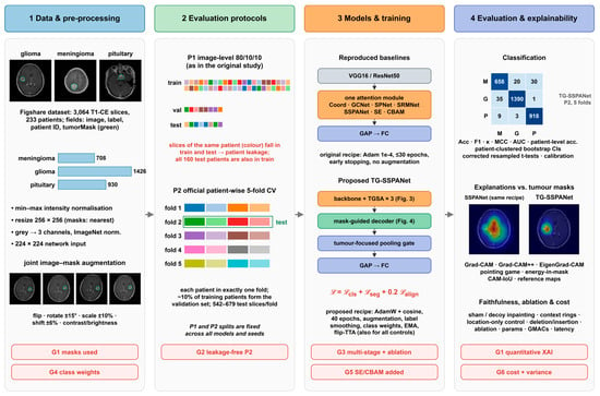
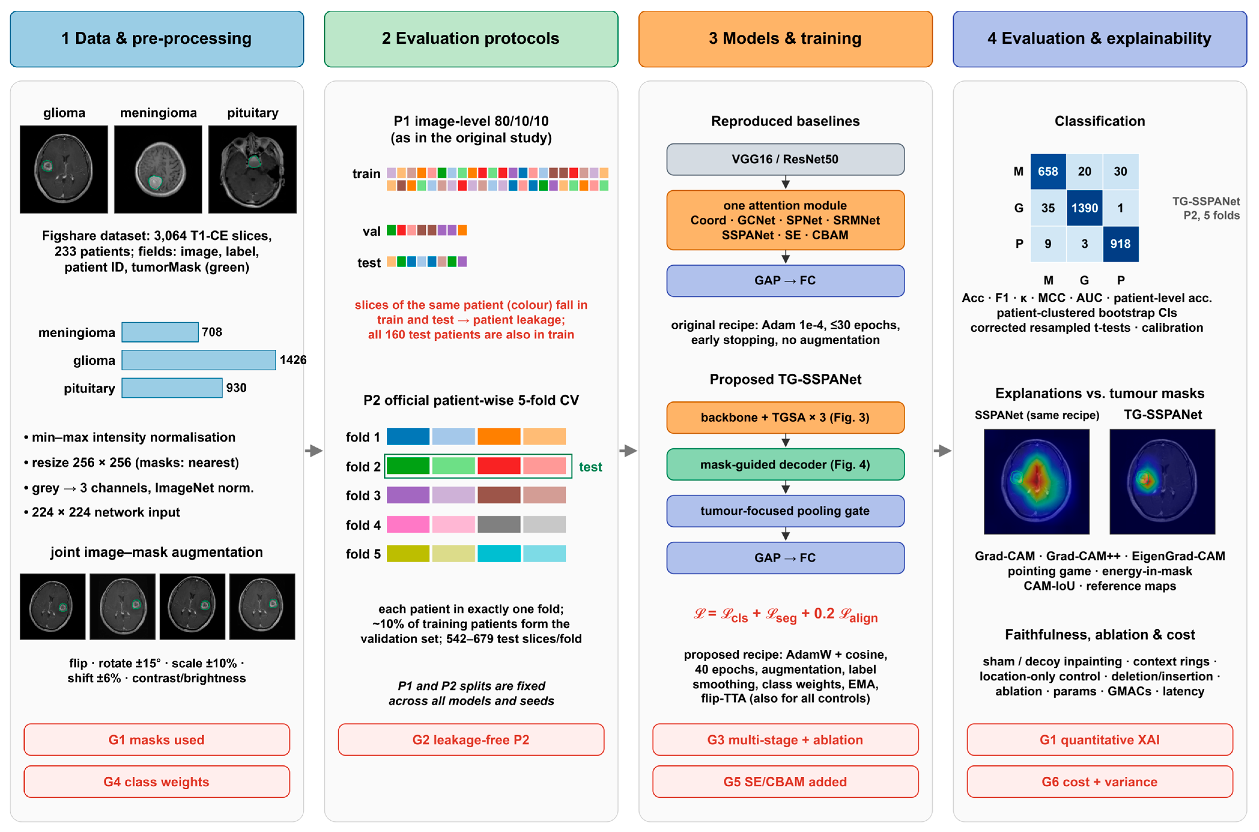
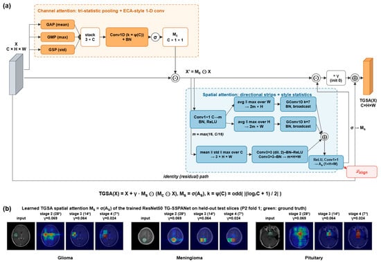
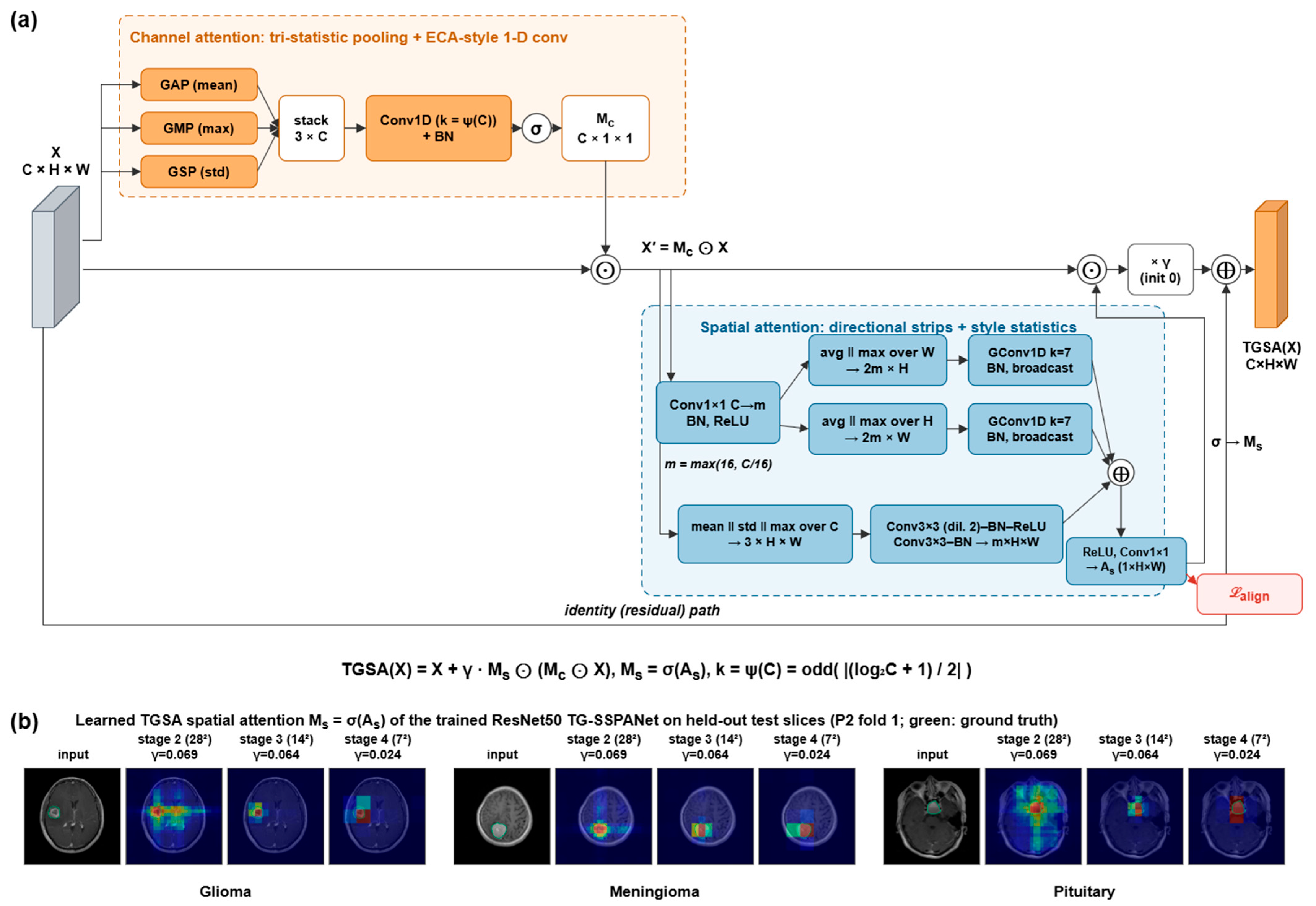
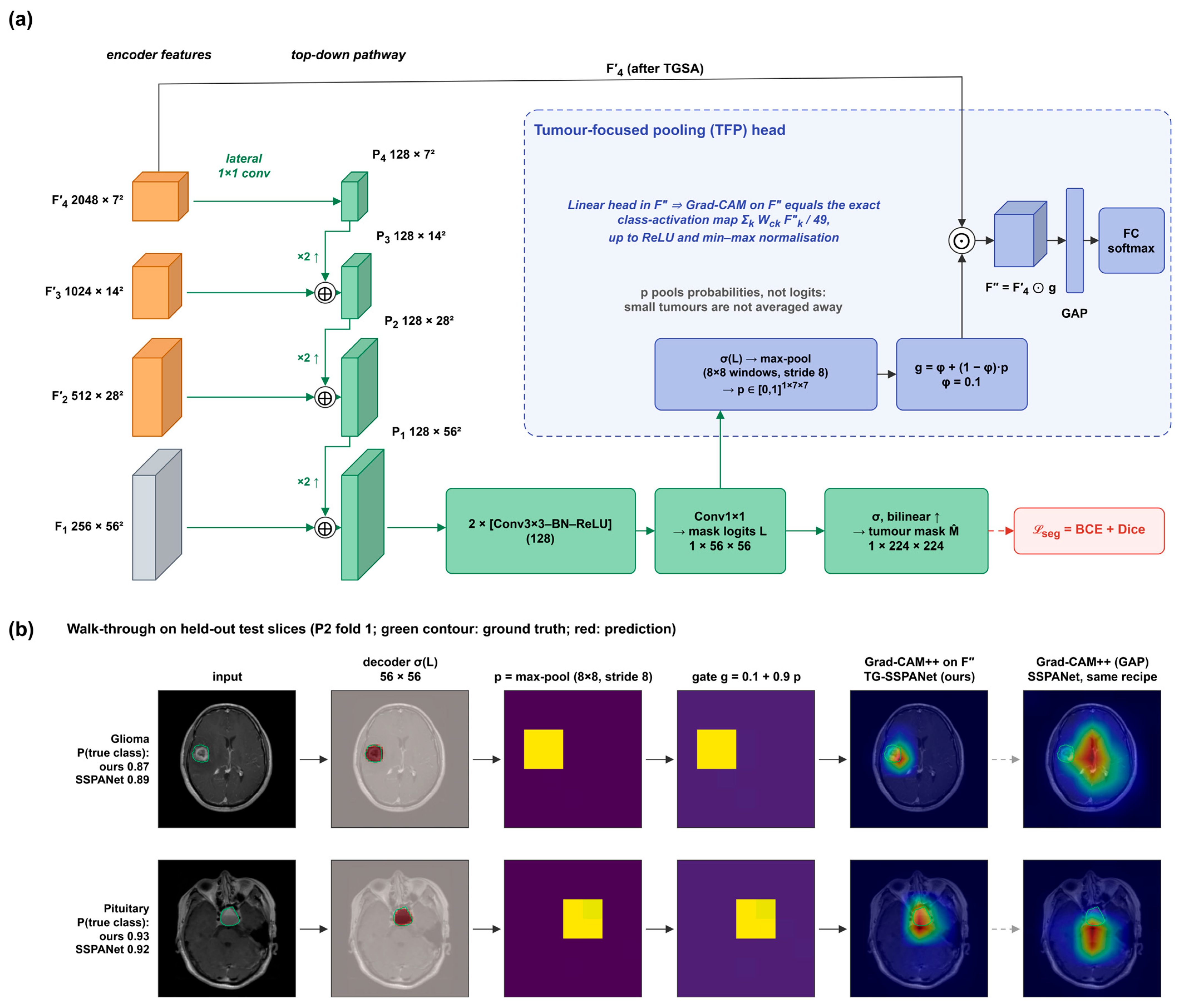
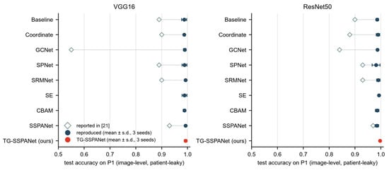
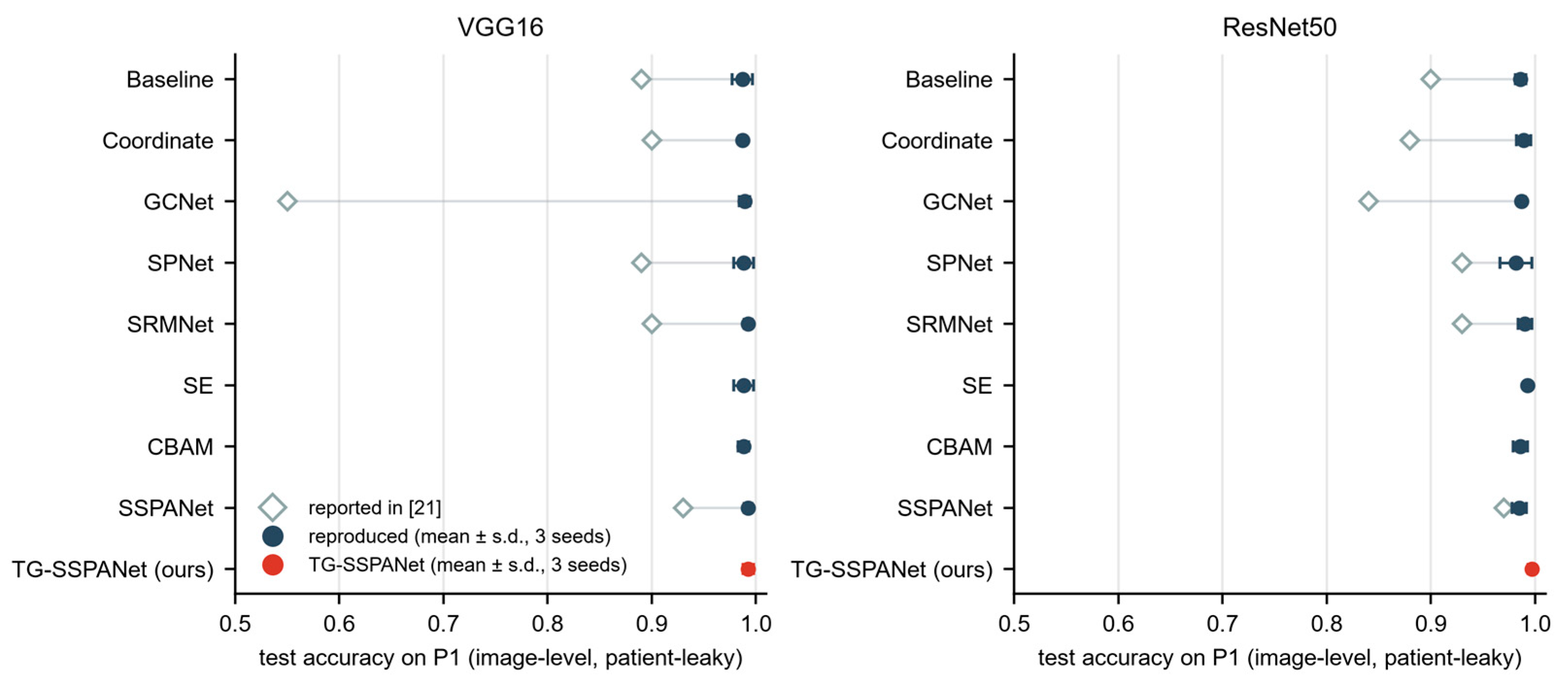
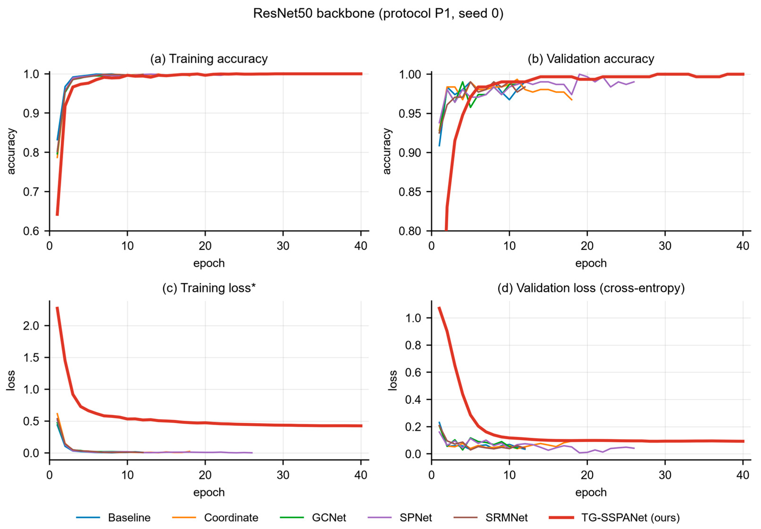
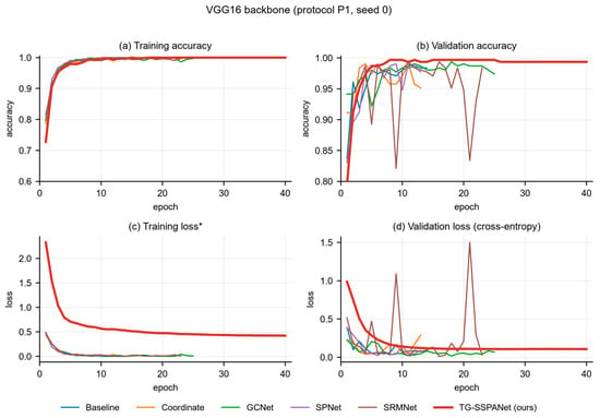
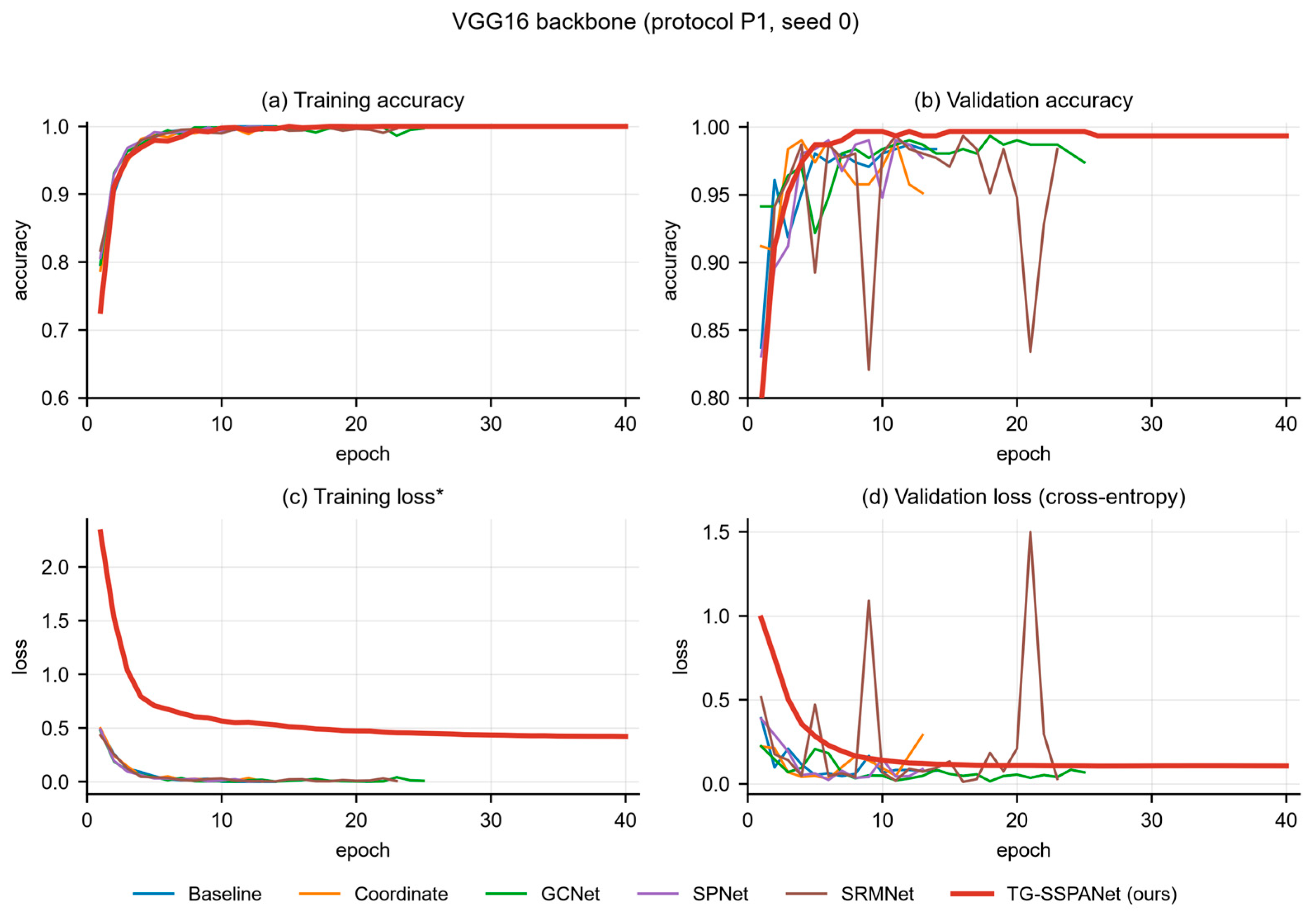
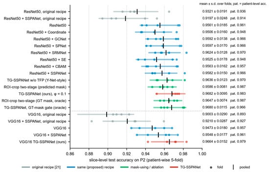
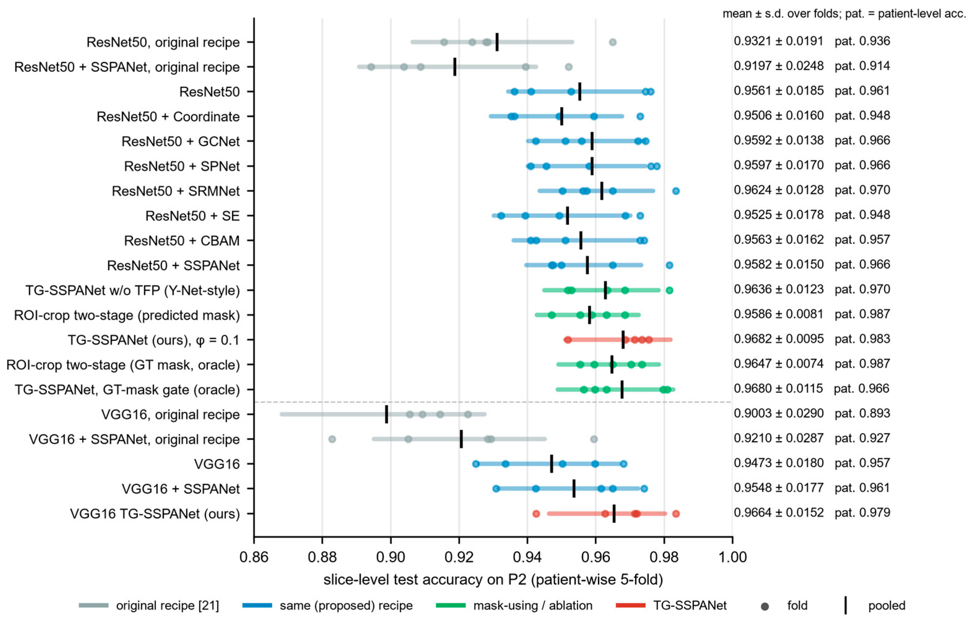
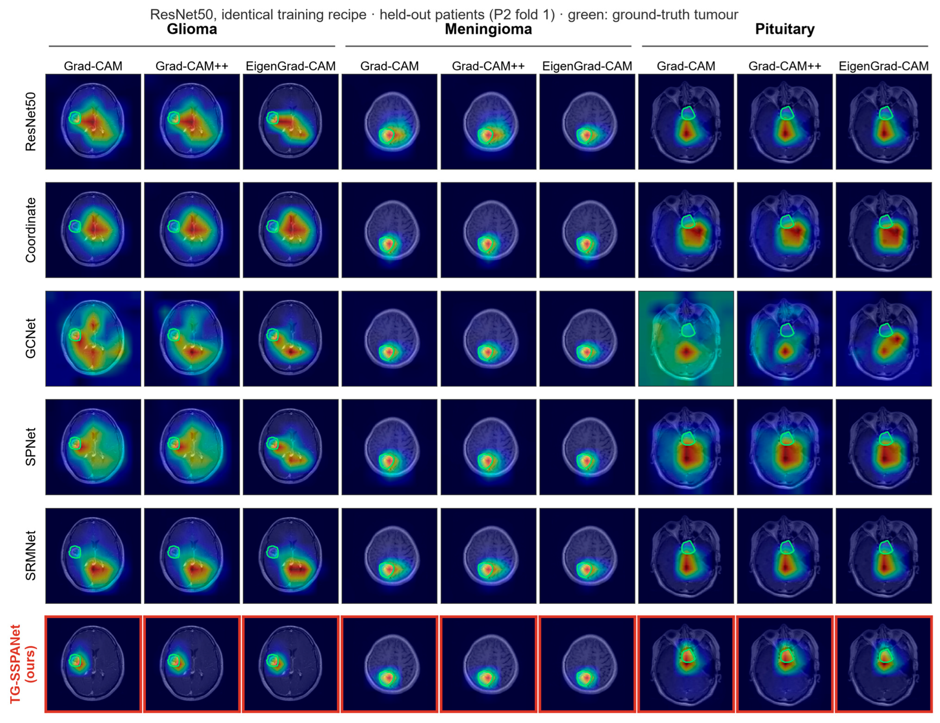
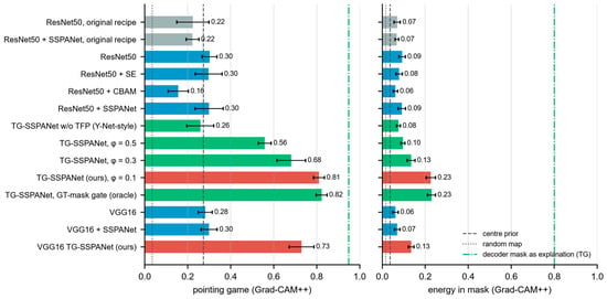
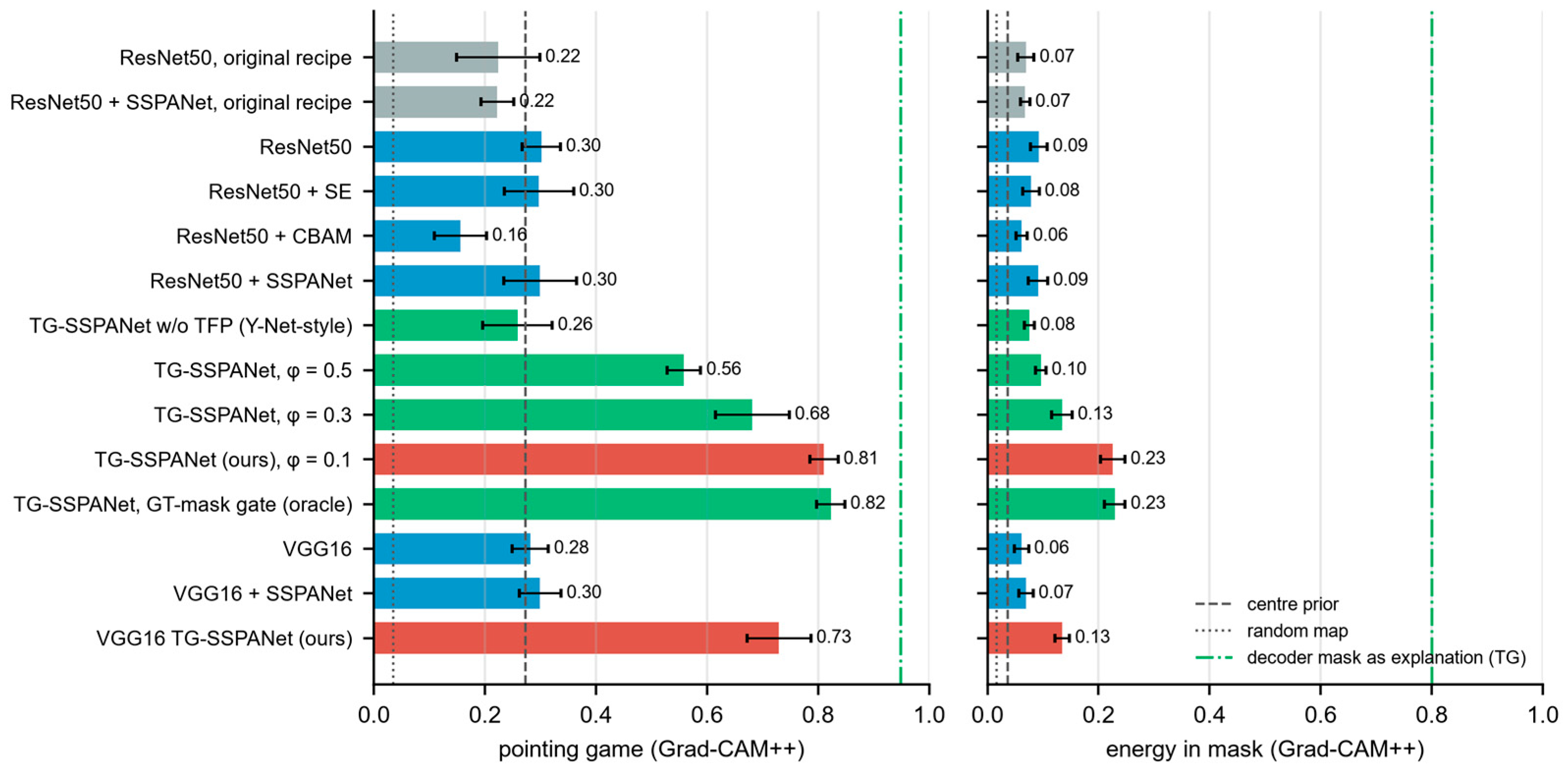
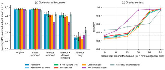
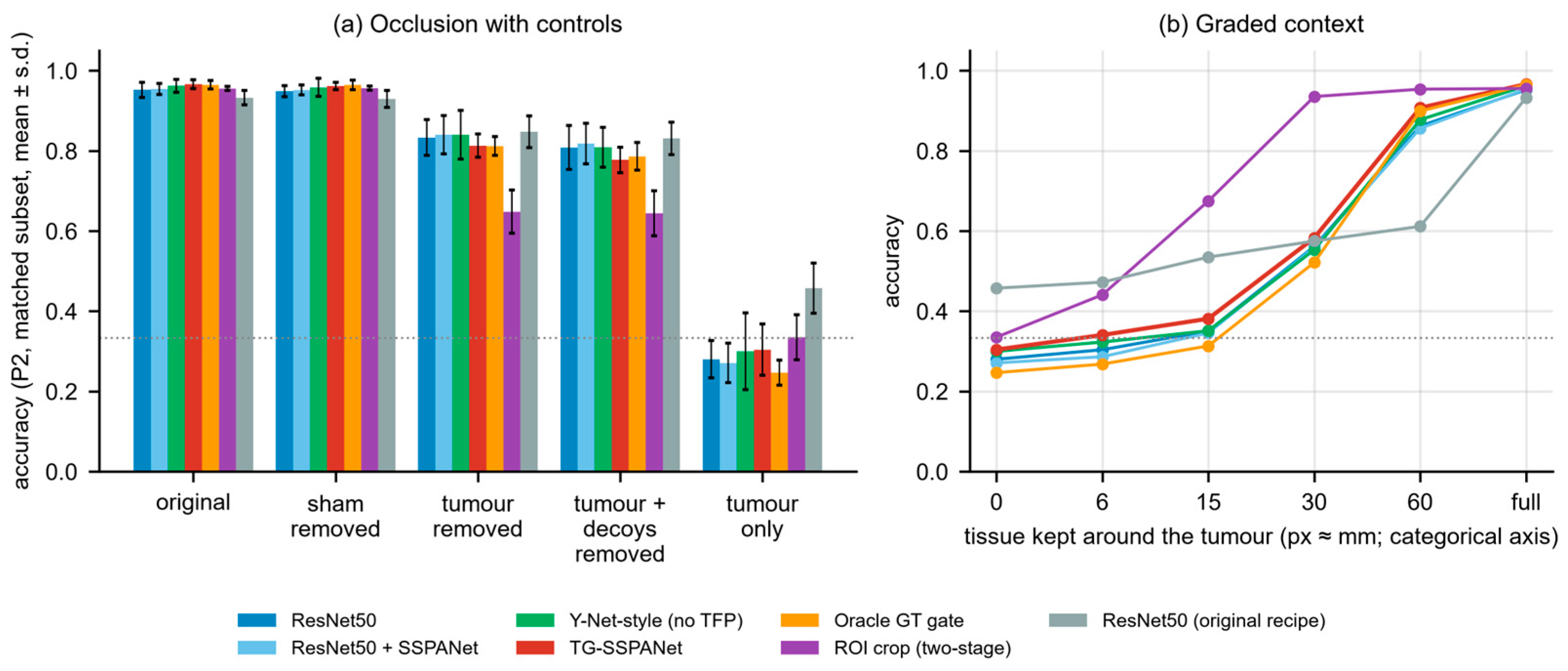
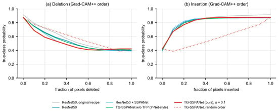
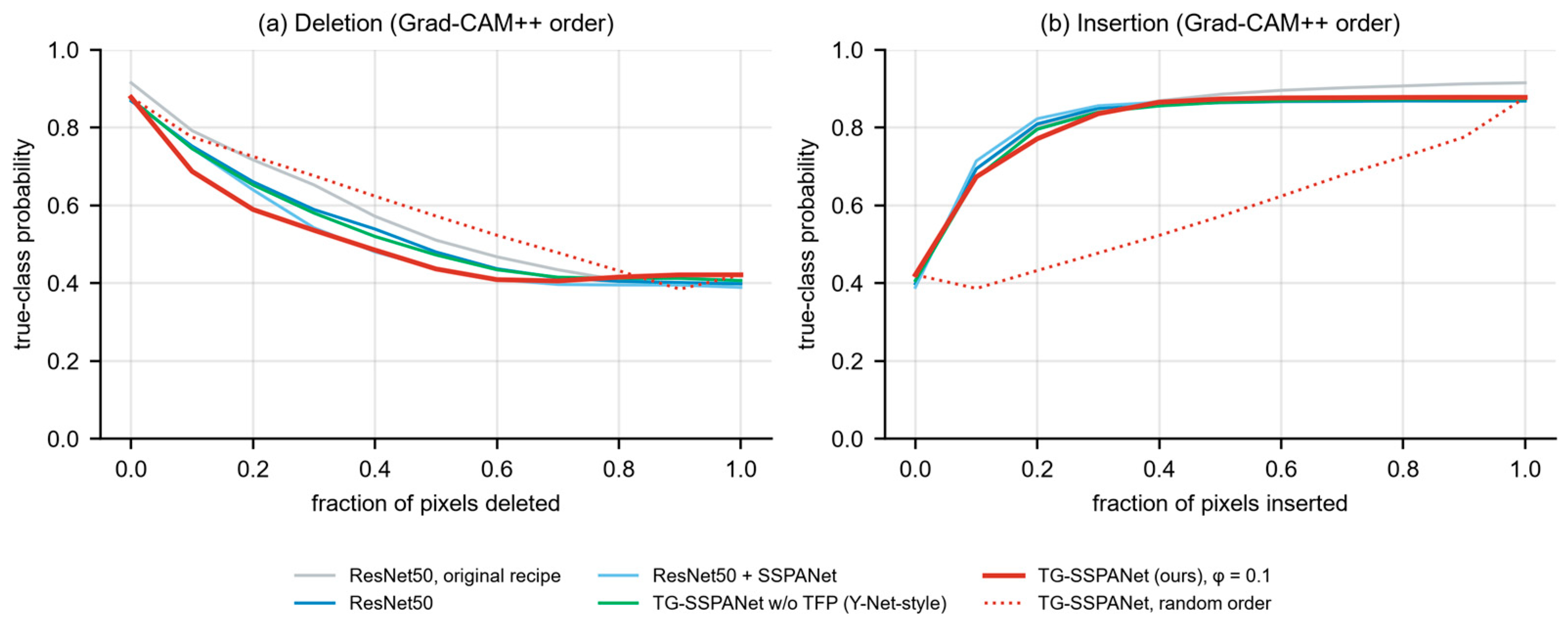
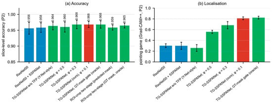
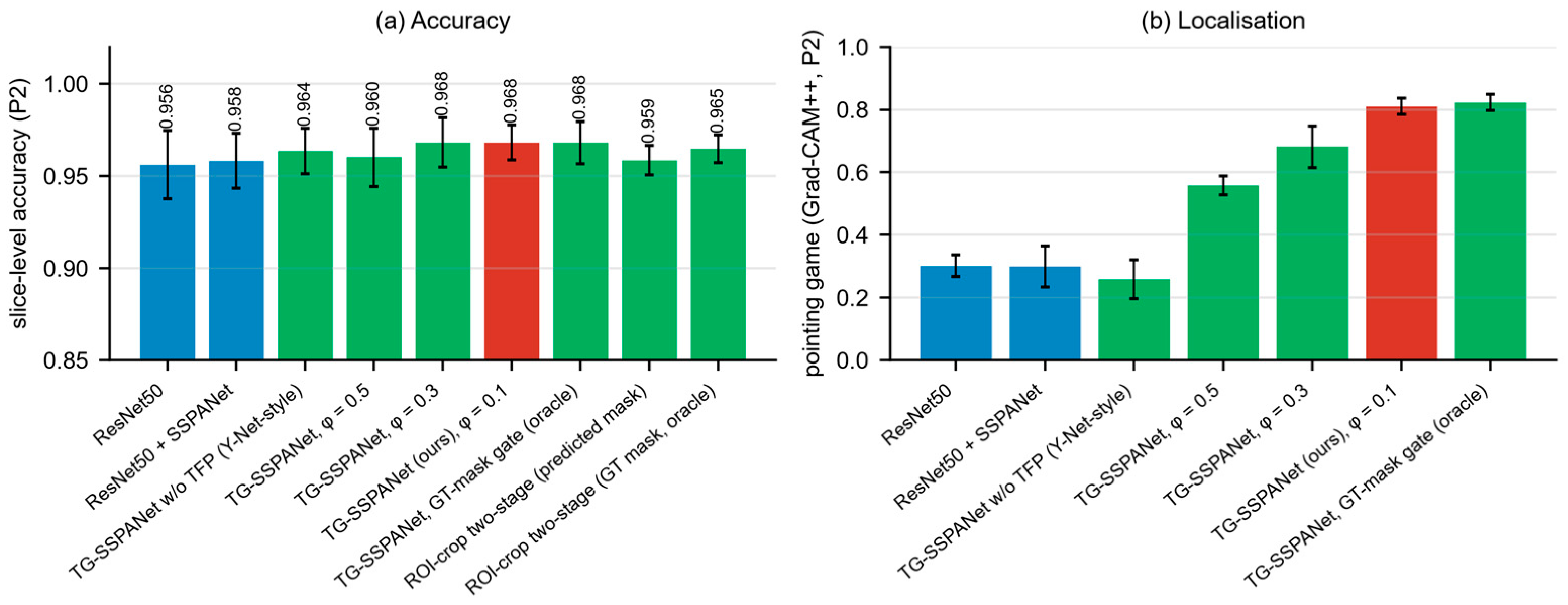
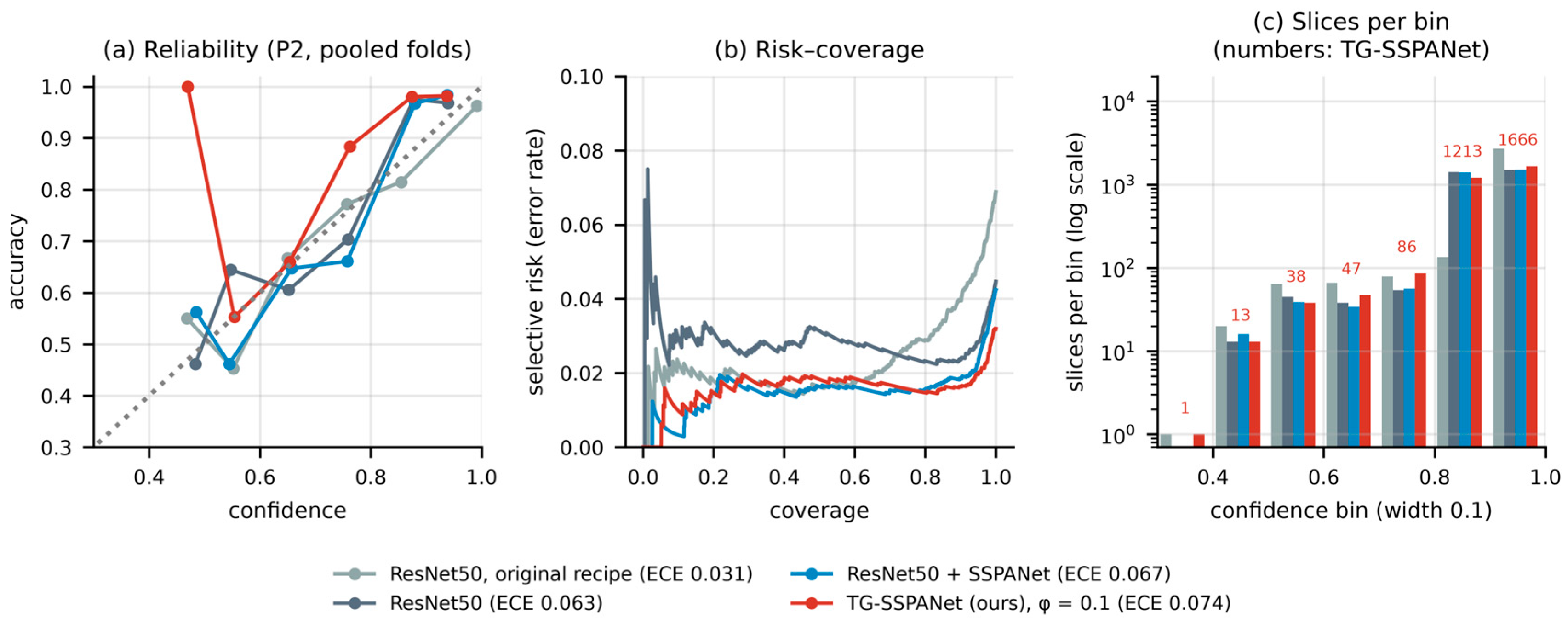
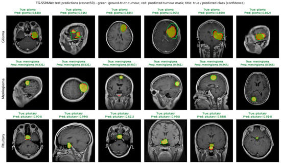
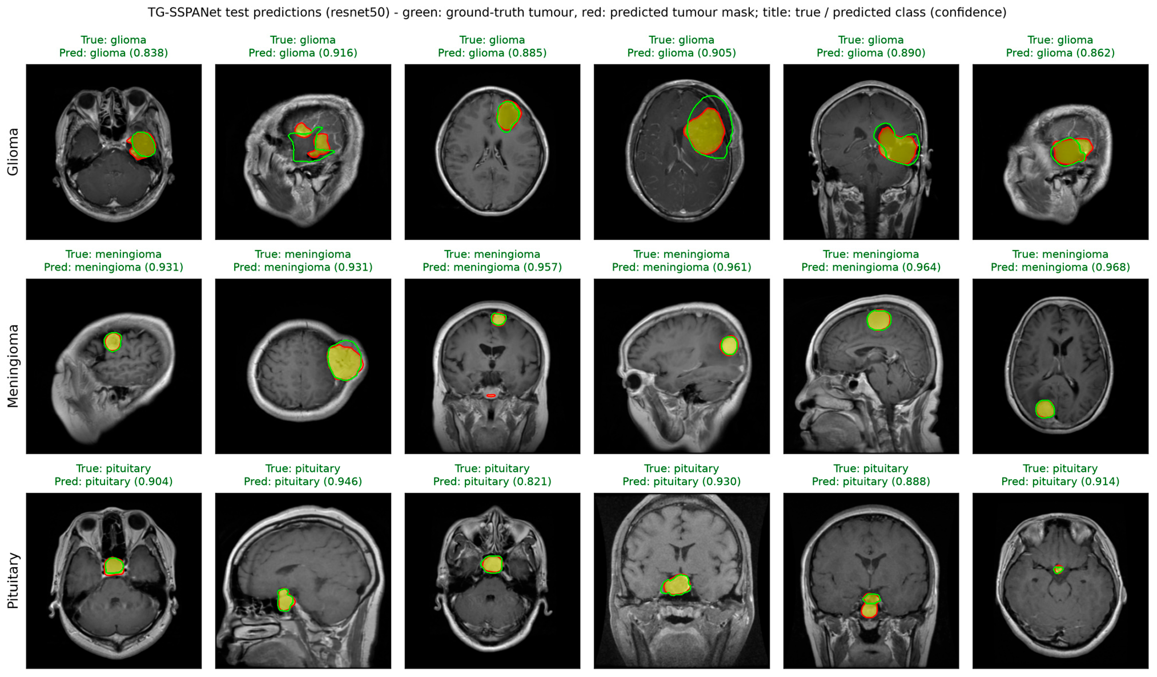
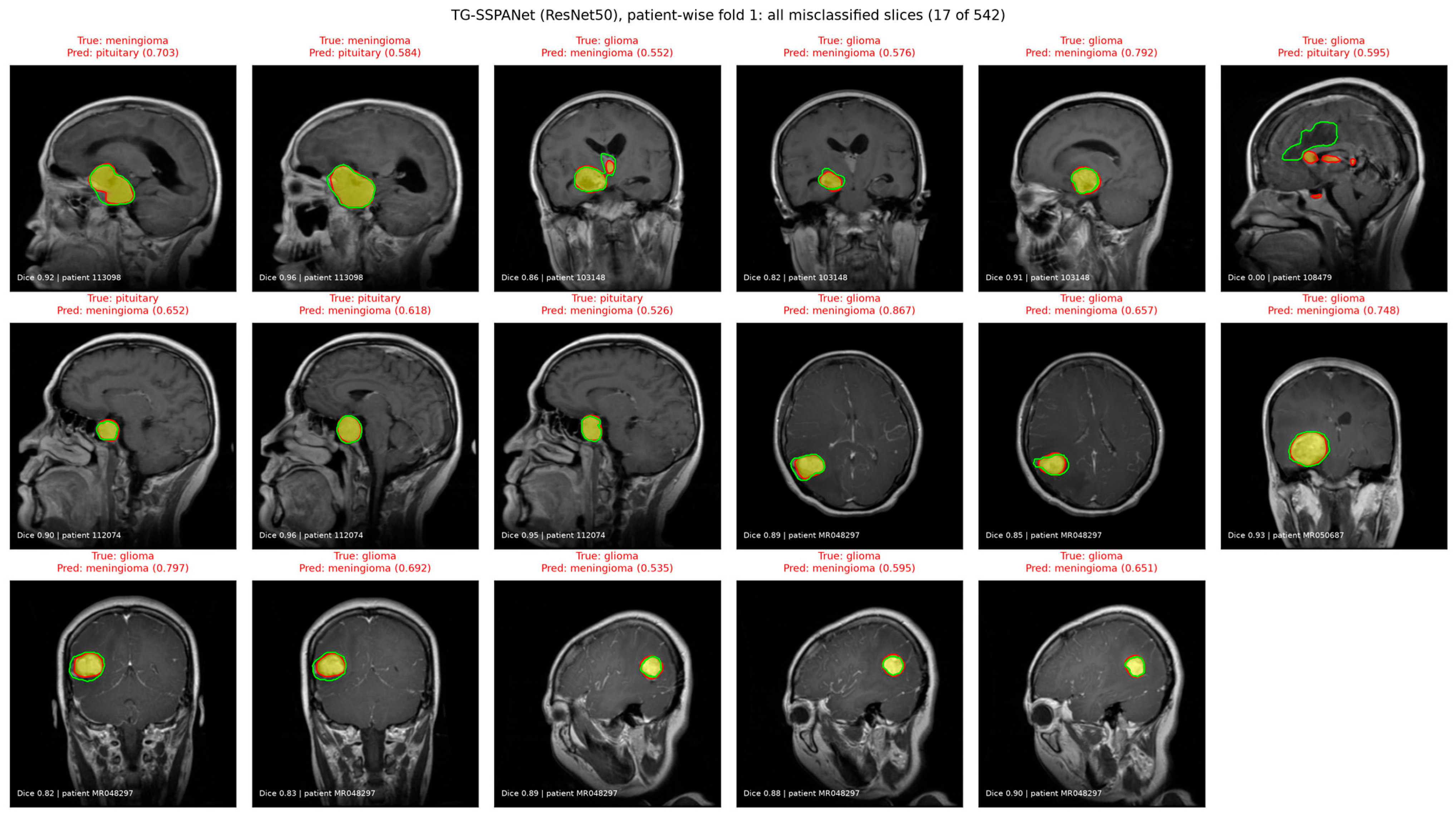

Disclaimer/Publisher’s Note: The statements, opinions and data contained in all publications are solely those of the individual author(s) and contributor(s) and not of MDPI and/or the editor(s). MDPI and/or the editor(s) disclaim responsibility for any injury to people or property resulting from any ideas, methods, instructions or products referred to in the content. |
© 2026 by the authors. Licensee MDPI, Basel, Switzerland. This article is an open access article distributed under the terms and conditions of the Creative Commons Attribution (CC BY) license.