Actor–Critic Predefined-Time Adaptive Tracking Control for Partially Unknown Euler–Lagrange Systems

Abstract

This paper studies predefined-time trajectory tracking for Euler–Lagrange systems with composite uncertainties encompassing partially known dynamics, parametric variations, and bounded disturbances. A two-step backstepping architecture is developed. In Step 1, a predefined-time virtual control law is constructed for the position subsystem. In Step 2, an energy-based torque controller is designed for the velocity subsystem using nominal model compensation, adaptive parameter estimation, actor neural network approximation of residual dynamics, a critic network for performance-oriented learning, and a continuous robust term. A rigorous Lyapunov analysis shows that all closed-loop signals are uniformly ultimately bounded and that the tracking errors converge to a computable residual set within a predefined time for all initial conditions contained in the selected compact set. Comparative simulations on a 2-DOF planar manipulator demonstrate that the proposed method provides faster convergence and improved steady-state tracking accuracy than both a PID baseline and a classical Slotine–Li adaptive baseline, while respecting the predefined-time bound.

1. Introduction

Predefined-time control aims to drive a system state to a target set within a user-assigned time bound that is independent of the initial condition [1]. For mechanical systems described by Euler–Lagrange (EL) dynamics, this property is attractive because trajectory tracking, path following, and cooperative manipulation frequently impose explicit transient requirements [2]. Practical implementation is nevertheless complicated by inaccurate inertial parameters, model-form effects such as friction and elasticity, bounded external disturbances, trajectory constraints, and actuator limitations [3,4,5]. These factors make it difficult to obtain a predefined-time guarantee without either requiring an exact dynamic model or introducing excessively conservative compensation.

Finite-time stability was systematically characterized by Bhat and Bernstein [6], with a settling time that generally depends on the initial state. Fixed-time stability subsequently removed this dependence and provided a uniform upper bound determined by controller parameters [7]. Predefined-time stability further allows the designer to assign the convergence-time parameter explicitly [8,9]. Related designs have been developed for general nonlinear systems [10], mechanical systems [11,12], distributed EL systems [2], robotic manipulators with neural approximation [13,14], flexible-joint robots with event-triggered implementation [15], and predefined-time EL systems with model uncertainties and actuator faults [3]. Although these studies substantially advance convergence speed analysis and robustness, many methods either employ exact or highly structured model cancellation, represent all uncertain dynamics by one lumped term, or do not separate the available nominal EL model from the residual model mismatch.

Adaptive control provides an effective mechanism for structured uncertainty. The classical Slotine–Li controller exploits the linear-in-parameters property of rigid-body dynamics to obtain asymptotic tracking [16]. Subsequent developments include leakage- and projection-based robust adaptive laws, composite learning methods, and neural approximators for unmodeled nonlinearities. Composite learning has been used to improve parameter convergence and tracking performance [17,18], while finite-time adaptive designs have addressed output constraints and uncertain robotic dynamics [19,20]. Adaptive predefined-time tracking has also been investigated for nonlinear systems with unmodeled dynamics [21]. Directly assigning the entire model error to one adaptive or neural approximator, however, does not exploit the common situation in which a reliable nominal rigid-body model is available together with structured parametric mismatch and a smaller nonparametric residual.

Reinforcement learning (RL) offers a complementary performance-oriented mechanism, and actor–critic architectures are widely used for continuous-state systems [22]. The actor generates a control or compensation signal, whereas the critic approximates a value function and supplies a long-term performance signal. Actor–critic methods have been developed through approximate dynamic programming and policy iteration formulations [23]. In robotic control, model-based actor–critic learning has been studied for optimal tracking under input saturation [24], for online PID tuning [25], and for energy-efficient manipulator control [26]. Most such approaches establish asymptotic, optimality-oriented, or uniformly ultimately bounded results rather than a user-assigned predefined-time tracking bound. Moreover, a Lyapunov-compatible critic must be specified through an explicit regressor, temporal-difference (TD) residual, update law, and bounded actor-coupling mechanism; its boundedness should not be imposed as an a priori assumption.

Recent reliability-oriented uncertainty studies have emphasized physics-guided learning, hierarchical decomposition, and dependency-aware surrogate modeling under limited data. Although these directions mainly address offline reliability assessment rather than closed-loop tracking, they motivate the separation of physically interpretable structures from learned residual components. Following the same modeling principle in an online control setting, the present work retains the nominal EL matrices in the implemented torque, identifies a structured parameter mismatch, approximates the remaining model-form residual by an actor network, and treats the final bounded remainder and exogenous disturbance with a continuous robust term. Thus, parametric, model-form, and disturbance uncertainties are not merged into one black-box channel.

The approaches that are closest to the present work differ in either their objective or their uncertainty treatment. The predefined-time mechanical system design in [12] establishes an initial condition-independent convergence bound but does not incorporate the structured-adaptive and actor–critic architecture considered here. The predefined-time EL controller in [3] addresses model uncertainty and actuator faults, whereas the present framework separates nominal compensation, structured parameter adaptation, neural residual approximation, and performance-oriented critic learning. The adaptive predefined-time design in [21] treats unmodeled nonlinearities in a general nonlinear system setting, while the controller developed here explicitly exploits the EL energy structure and uses only the nominal inertia matrix in its online predefined-time damping. Conversely, the robot actor–critic methods in [24,26] pursue optimal or energy-efficient tracking without deriving the practical predefined-time Lyapunov inequality used here.

To address these gaps, this paper proposes an actor–critic predefined-time adaptive tracking controller for partially unknown EL systems. The main contributions are summarized as follows:

(i)

An implementable two-step backstepping architecture is developed using only the known nominal matrices $H_0\left(q\right)$, $C_0(q,\dot{q})$, and $g_0\left(q\right)$. The true–nominal mismatch is decomposed into a structured parametric term, an actor-approximated residual term, and a bounded remainder handled by a continuous hyperbolic-tangent robust term. The unknown true inertia matrix is used only in the Lyapunov analysis and not in the online controller.

(ii)

An explicit continuous-time actor–critic mechanism is integrated with the adaptive controller. The critic regressor $\Lambda \left(Z_c\right)$ and TD residual are specified directly, and a bounded squared TD residual gate modulates the stabilizing tracking-driven actor update without reversing its direction or depending on an arbitrary offset of the approximate value function. Critic boundedness is established through the TD term, leakage, and dual-power regularization rather than being imposed as an a priori boundedness assumption.

(iii)

A composite Lyapunov analysis includes predefined-time dual-power dissipation for the position, velocity, structured-parameter, actor, and critic error components. The aggregation is therefore applied to the complete Lyapunov function. The analysis establishes semi-global uniform ultimate boundedness and gives an explicit analytical residual-bound expression in terms of the derived constants, which can be numerically evaluated once the proof constants are instantiated.

The remainder of this paper is organized as follows. Section 2 introduces the EL system and formulates the tracking problem. Section 3 presents the assumptions and preliminary lemmas. Section 4 develops the controller and adaptive actor–critic laws. Section 5 states and proves the main result. Section 6 presents the numerical study, and Section 7 concludes the paper.

2. System Description and Problem Formulation

2.1. Euler–Lagrange Dynamics

Consider the n-DOF Euler–Lagrange system

$$H\left(q\right)\ddot{q}+C(q,\dot{q})\dot{q}+g\left(q\right)=\tau +d\left(t\right),$$

(1)

where $q,\dot{q},\ddot{q}\in {\mathbb{R}}^n$ are the generalized position, velocity, and acceleration vectors, respectively; $H\left(q\right)\in {\mathbb{R}}^{n\times n}$ is the inertia matrix; $C(q,\dot{q})\in {\mathbb{R}}^{n\times n}$ is the Coriolis/centripetal matrix; $g\left(q\right)\in {\mathbb{R}}^n$ is the gravity vector; $\tau \in {\mathbb{R}}^n$ is the control torque; and $d\left(t\right)\in {\mathbb{R}}^n$ is a bounded disturbance.

We assume that the rigid-body structure of the system is available, so that nominal matrices $H_0\left(q\right)$, $C_0(q,\dot{q})$, and $g_0\left(q\right)$ can be constructed. The true system may differ from the nominal model because of structured parameter mismatch, residual model-form uncertainty, and bounded disturbances.

2.2. Tracking Objective

Let $q_d\left(t\right)\in {\mathbb{R}}^n$ be a sufficiently smooth desired trajectory. Define the position tracking error

$$z_1\triangleq q-q_d.$$

(2)

The control objective is to design a continuous torque input $\tau \left(t\right)$ and adaptive laws such that

(i)

all closed-loop signals remain bounded for all $t\ge 0$;

(ii)

the tracking errors converge to a small residual set in predefined time;

(iii)

the adaptive estimates remain bounded and compensate for structured and residual uncertainty online.

3. Assumptions and Preliminary Lemmas

3.1. Assumptions

Assumption 1.

For all $q\in {\mathbb{R}}^n$, the inertia matrix $H\left(q\right)$ is symmetric positive definite, and there exist known constants $0<c_0\le c_1$ such that

$$c_0{I}_n\le H\left(q\right)\le c_1{I}_n.$$

(3)

Moreover, the skew-symmetry property holds:

$${\xi }^{\top }\left(\dot{H}\left(q\right)-2C(q,\dot{q})\right)\xi =0,\forall \xi \in {\mathbb{R}}^n.$$

(4)

Assumption 2.

The nominal matrices $H_0\left(q\right)$, $C_0(q,\dot{q})$, and $g_0\left(q\right)$ are known and continuous. There exists a known constant ${\underline{h}}_0>0$ such that

$$z^{\top }{H}_0\left(q\right)z\ge {\underline{h}}_0{\parallel z\parallel }^2,\forall z\in {\mathbb{R}}^n,\forall q.$$

(5)

Assumption 3.

The desired trajectory $q_d\left(t\right)$ is twice continuously differentiable, and there exist known constants ${\overline{v}}_d,{\overline{a}}_d>0$ such that

$$\underset{t\ge 0}{sup}\parallel {\dot{q}}_d\left(t\right)\parallel \le {\overline{v}}_d,\underset{t\ge 0}{sup}\parallel {\ddot{q}}_d\left(t\right)\parallel \le {\overline{a}}_d.$$

(6)

Assumption 4.

The disturbance satisfies

$$\parallel d\left(t\right)\parallel \le \overline{d},\forall t\ge 0,$$

(7)

for a known constant $\overline{d}>0$.

Assumption 5.

Let

$${\delta }_f\triangleq {\dot{\alpha }}_1-v_{1f},$$

(8)

where $v_{1f}$ is the command-filter output approximating ${\dot{\alpha }}_1$. Define

$$Z\triangleq col\left(q,\dot{q},q_d,{\dot{q}}_d,{\ddot{q}}_d,{\alpha }_1,{\alpha }_{1f},v_{1f}\right)$$

(9)

and the lumped model mismatch

$$\begin{array}{cc}\hfill \Delta \left(Z\right)\triangleq & H\left(q\right){\delta }_f+\left(H\left(q\right)-H_0\left(q\right)\right)v_{1f}\hfill \\ \hfill & +\left(C(q,\dot{q})-C_0(q,\dot{q})\right){\alpha }_1+\left(g\left(q\right)-g_0\left(q\right)\right).\hfill \end{array}$$

(10)

For any prescribed compact approximation domain ${\Omega }_a$ of Z, there exist a known continuous regressor $Y\left(Z\right)\in {\mathbb{R}}^{n\times p}$, an unknown constant parameter vector ${\theta }^{*}\in {\mathbb{R}}^p$, an unknown constant ideal actor weight matrix $W_a^{*}\in {\mathbb{R}}^{{\ell }_a\times n}$, a continuously differentiable RBF basis vector $S_a\left(Z\right)\in {\mathbb{R}}^{{\ell }_a}$, and an approximation residual ${\epsilon }_a\left(Z\right)\in {\mathbb{R}}^n$ such that

$$\Delta \left(Z\right)=Y\left(Z\right){\theta }^{*}+{\left(W_a^{*}\right)}^{\top }{S}_a\left(Z\right)+{\epsilon }_a\left(Z\right),Z\in {\Omega }_a.$$

(11)

Furthermore, there exist known constants $\overline{\theta },{\overline{W}}_a,\overline{Y},{\overline{S}}_a,{\overline{\epsilon }}_a>0$ satisfying

$$\parallel {\theta }^{*}\parallel \le \overline{\theta },{\parallel W_a^{*}\parallel }_F\le {\overline{W}}_a,$$

(12)

and

$$\parallel Y\left(Z\right)\parallel \le \overline{Y},\parallel S_a\left(Z\right)\parallel \le {\overline{S}}_a,\parallel {\epsilon }_a\left(Z\right)\parallel \le {\overline{\epsilon }}_a.$$

(13)

Assumption 6.

Let

$$Z_c\triangleq col(z_1,z_2)$$

(14)

be the critic input. For any prescribed compact approximation domain ${\Omega }_c$ of $(Z_c,{\dot{Z}}_c)$, there exist a constant ideal critic weight vector $W_c^{*}$ and a continuously differentiable basis vector $S_c\left(Z_c\right)$ such that the approximate Hamilton–Jacobi–Bellman relation

$$\varphi \left(t\right)+{\left(W_c^{*}\right)}^{\top }\Lambda \left(Z_c\right)={\epsilon }_B\left(Z_c\right)$$

(15)

holds, where

$$\Lambda \left(Z_c\right)\triangleq {\displaystyle \frac{\partial S_c\left(Z_c\right)}{\partial Z_c}}{\dot{Z}}_c.$$

(16)

There exist known constants ${\overline{W}}_c,{\overline{S}}_c,\overline{\Lambda },{\overline{\epsilon }}_B>0$ such that

$$\parallel W_c^{*}\parallel \le {\overline{W}}_c,\parallel S_c\left(Z_c\right)\parallel \le {\overline{S}}_c,$$

(17)

and

$$\parallel \Lambda \left(Z_c\right)\parallel \le \overline{\Lambda },|{\epsilon }_B\left(Z_c\right)|\le {\overline{\epsilon }}_B,(Z_c,{\dot{Z}}_c)\in {\Omega }_c.$$

(18)

Remark 1.

Assumptions 5 and 6 impose approximation properties on designer-selected compact domains; they do not assume a priori that all closed-loop signals are bounded. For any prescribed compact set of initial conditions, the domains ${\Omega }_a$ and ${\Omega }_c$ are selected to contain the corresponding Lyapunov sublevel set. The continuation argument in the proof shows that the trajectory cannot leave this sublevel set. The resulting stability statement is therefore semi-global and practical.

3.2. Preliminary Lemmas

Lemma 1

([8]). Let $V\left(t\right)\ge 0$ be continuously differentiable. If there exist constants $T_c>0$, $0<\beta <1$, and $\sigma \ge 0$ such that

$$\dot{V}\le -{\displaystyle \frac{\pi }{\beta T_c}}\left(V^{1-\beta /2}+V^{1+\beta /2}\right)+\sigma ,$$

(19)

then $V\left(t\right)$ converges to a residual set in a time

$$T_P<\sqrt{2}{T}_c$$

(20)

for all initial conditions contained in the selected compact set.

Lemma 2.

For any $x\in \mathbb{R}$ and $\rho >0$,

$$0\le |x|-xtanh(x/\rho )\le 0.2785\rho .$$

(21)

Consequently, for any $z\in {\mathbb{R}}^n$,

$$0\le {\parallel z\parallel }_1-z^{\top }tanh(z/\rho )\le 0.2785n\rho ,$$

(22)

where $tanh(z/\rho )$ is applied componentwise.

Lemma 3.

Let $V_i\ge 0$ for $i=1,\dots ,m$, and let $V={\sum }_{i=1}^m{V}_i$. Then, for any $0<\beta <1$,

$${\displaystyle \sum _{i=1}^m}\left(V_i^{1-\beta /2}+V_i^{1+\beta /2}\right)\ge {\kappa }_m\left(V^{1-\beta /2}+V^{1+\beta /2}\right),$$

(23)

where

$${\kappa }_m=m^{-\beta /2}.$$

(24)

Lemma 4.

For a scalar, vector, or matrix estimate $\widehat{p}$, define the componentwise dual-power mapping

$${\mathcal{R}}_{\beta }\left(\widehat{p}\right)\triangleq |\widehat{p}{|}^{-\beta }\odot \widehat{p}+{|\widehat{p}|}^{\beta }\odot \widehat{p},0<\beta <1,$$

(25)

where ${|0|}^{-\beta }0$ is defined as zero. Let $\tilde{p}=p^{*}-\widehat{p}$, where $p^{*}$ is constant, and define

$$V_p={\displaystyle \frac{1}{2r_p}}{\parallel \tilde{p}\parallel }^2$$

(26)

for vectors or the analogous Frobenius norm expression for matrices. Then, there exist constants ${\underline{c}}_p>0$ and ${\overline{C}}_p\ge 0$ such that

$${\displaystyle \frac{c_p}{r_p}}⟨\tilde{p},{\mathcal{R}}_{\beta }\left(\widehat{p}\right)⟩\le -{\underline{c}}_p\left(V_p^{1-\beta /2}+V_p^{1+\beta /2}\right)+{\overline{C}}_p.$$

(27)

Here, $⟨·,·⟩$ denotes the Euclidean inner product for vectors and the Frobenius inner product for matrices.

Remark 2.

The two components of ${\mathcal{R}}_{\beta }(·)$ have distinct roles: $|\widehat{p}{|}^{-\beta }\odot \widehat{p}$ generates the subquadratic Lyapunov power, whereas $|\widehat{p}{|}^{\beta }\odot \widehat{p}$ generates the superquadratic Lyapunov power. Both components are therefore retained in the structured-parameter, actor, and critic update laws used below.

4. Actor–Critic Predefined-Time Controller Design

Define the position tracking error

$$z_1=q-q_d.$$

(28)

For each component $z_{1,i}$, define the predefined-time kernel

$${\widehat{\alpha }}_{1,i}\left(z_{1,i}\right)\triangleq {\displaystyle \frac{\pi {\kappa }_1}{\beta T_c}}\left[2^{\beta /2}|z_{1,i}{|}^{1+\beta }sign\left(z_{1,i}\right)+2^{-\beta /2}{|z_{1,i}|}^{1-\beta }sign\left(z_{1,i}\right)\right],$$

(29)

where $T_c>0$ is the user-specified time parameter, $0<\beta <1$, and ${\kappa }_1>0$ is a design gain. The smooth virtual control is

$${\alpha }_1=-{\displaystyle \frac{z_1\odot {\widehat{\alpha }}_1^2}{\sqrt{z_1^2\odot {\widehat{\alpha }}_1^2+{\epsilon }_1^2{\mathbf{1}}_n}}}+{\dot{q}}_d,$$

(30)

where ${\widehat{\alpha }}_1={[{\widehat{\alpha }}_{1,1},\dots ,{\widehat{\alpha }}_{1,n}]}^{\top }$ and ${\epsilon }_1>0$ is a smoothing constant. All vector powers, products, divisions, and square roots in (30) are applied componentwise.

To avoid the direct differentiation of ${\alpha }_1$, introduce the second-order command filter

$${\dot{\alpha }}_{1f}=v_{1f},{\dot{v}}_{1f}=-2{\omega }_f{v}_{1f}-{\omega }_f^2({\alpha }_{1f}-{\alpha }_1),$$

(31)

where ${\omega }_f>0$, with ${\alpha }_{1f}\left(0\right)={\alpha }_1\left(0\right)$ and $v_{1f}\left(0\right)=0$. The derivative approximation error is

$${\delta }_f={\dot{\alpha }}_1-v_{1f}.$$

(32)

Define the velocity error

$$z_2=\dot{q}-{\alpha }_1.$$

(33)

For Lyapunov analysis, introduce the true mechanical energy

$$V_2={\displaystyle \frac{1}{2}}{z}_2^{\top }H\left(q\right)z_2.$$

(34)

The quantity in (34) is used only in the proof. For online implementation, define the nominal energy

$$V_{20}={\displaystyle \frac{1}{2}}{z}_2^{\top }{H}_0\left(q\right)z_2$$

(35)

and the implementable predefined-time scaling

$${\Pi }_0\left(V_{20}\right)\triangleq {\displaystyle \frac{\pi {\kappa }_2}{\beta T_c}}\left(V_{20}^{-\beta /2}+V_{20}^{\beta /2}\right),V_{20}>0.$$

(36)

At $z_2=0$, the product ${\Pi }_0\left(V_{20}\right)H_0\left(q\right)z_2$ is defined by its continuous extension as zero.

The commanded torque is

$$\begin{array}{cc}\hfill \tau =& H_0\left(q\right)v_{1f}+C_0(q,\dot{q}){\alpha }_1+g_0\left(q\right)-z_1\hfill \\ \hfill & -K_2{H}_0\left(q\right)z_2-K_{pt}{\Pi }_0\left(V_{20}\right)H_0\left(q\right)z_2+Y\left(Z\right)\widehat{\theta }\hfill \\ \hfill & +{\widehat{W}}_a^{\top }{S}_a\left(Z\right)-k_{r}tanh(z_2/\rho ),\hfill \end{array}$$

(37)

where $K_2,K_{pt},k_r,\rho >0$, and $tanh(·)$ is applied componentwise.

Remark 3.

The unknown true matrix $H\left(q\right)$ is not required online. It appears only in (34). The implemented predefined-time damping uses the measurable nominal energy $V_{20}$ and the known matrix $H_0\left(q\right)$. The relation between $V_{20}$ and $V_2$ is invoked only in the stability analysis.

Define the structured parameter estimation error

$$\tilde{\theta }={\theta }^{*}-\widehat{\theta }.$$

(38)

The structured adaptive law is

$$\dot{\widehat{\theta }}=-r_{\theta }Y{\left(Z\right)}^{\top }{z}_2-{\sigma }_{\theta }\widehat{\theta }-c_{\theta }{\mathcal{R}}_{\beta }\left(\widehat{\theta }\right),$$

(39)

where $r_{\theta },{\sigma }_{\theta },c_{\theta }>0$.

For the residual nonlinear mismatch, define

$${\tilde{W}}_a=W_a^{*}-{\widehat{W}}_a.$$

(40)

The instantaneous cost is

$$\varphi \left(t\right)=Q_1\parallel z_1{\parallel }^2+Q_2\parallel z_2{\parallel }^2+R{\parallel \tau \parallel }^2,$$

(41)

where $Q_1,Q_2,R>0$. The critic provides an auxiliary long-term performance evaluation signal as

$$J\left(Z_c\right)\approx {\widehat{W}}_c^{\top }{S}_c\left(Z_c\right).$$

(42)

For $Z_c=col(z_1,z_2)$,

$${\dot{Z}}_c=col\left(z_2+{\alpha }_1-{\dot{q}}_d,\ddot{q}-{\dot{\alpha }}_1\right).$$

(43)

The temporal-difference residual is

$${\delta }_{\mathrm{TD}}=\varphi \left(t\right)+{\widehat{W}}_c^{\top }\Lambda \left(Z_c\right),$$

(44)

where $\Lambda \left(Z_c\right)$ is defined in (16). By Assumption 6 and ${\tilde{W}}_c=W_c^{*}-{\widehat{W}}_c$,

$${\delta }_{\mathrm{TD}}=-{\tilde{W}}_c^{\top }\Lambda \left(Z_c\right)+{\epsilon }_B\left(Z_c\right).$$

(45)

To provide a bounded critic-to-actor channel, define

$$g_c\left({\delta }_{\mathrm{TD}}\right)\triangleq {\displaystyle \frac{{\delta }_{\mathrm{TD}}^2}{{\delta }_{\mathrm{TD}}^2+{\delta }_0^2}},{\delta }_0>0,$$

(46)

so that $0\le g_c<1$, and define the effective actor learning rate

$$r_a^{\mathrm{eff}}\triangleq r_a\left[1+K_I{g}_c\left({\delta }_{\mathrm{TD}}\right)\right],K_I\ge 0.$$

(47)

The actor update law is

$${\dot{\widehat{W}}}_a=-r_a^{\mathrm{eff}}{S}_a\left(Z\right)z_2^{\top }-{\sigma }_a{\widehat{W}}_a-c_a{\mathcal{R}}_{\beta }\left({\widehat{W}}_a\right),$$

(48)

where $r_a,{\sigma }_a,c_a>0$.

Remark 4.

The gate in (46) is nonnegative, bounded, and invariant to an additive offset of the approximate value function. It increases the magnitude of the stabilizing tracking-driven actor update when the TD residual is large, but it cannot reverse the direction of this update. For $K_I=0$, or when the critic is removed, (48) reduces to the corresponding actor-only law.

The critic update law is

$${\dot{\widehat{W}}}_c=-r_c\Lambda \left(Z_c\right){\delta }_{\mathrm{TD}}-{\sigma }_c{\widehat{W}}_c-c_c{\mathcal{R}}_{\beta }\left({\widehat{W}}_c\right),$$

(49)

where $r_c,{\sigma }_c,c_c>0$.

Remark 5.

For the continuous-time analysis, $\Lambda =(\partial S_c/\partial Z_c){\dot{Z}}_c$. In the numerical implementation, a stable first-order filter ${\dot{\widehat{\dot{Z}}}}_c={\omega }_{\Lambda }({\dot{Z}}_c-{\widehat{\dot{Z}}}_c)$ is used and $\Lambda =(\partial S_c/\partial Z_c){\widehat{\dot{Z}}}_c$. The resulting filter error is included in the bounded Bellman residual ${\epsilon }_B$. The same filtered differentiation construction can be used in an experimental implementation.

5. Main Result

Theorem 1.

Consider the Euler–Lagrange system (1) under Assumptions 1–6. Apply the virtual control (30), command filter (31), torque law (37), and update laws (39), (48), and (49). For any prescribed compact set of initial conditions contained in the selected approximation domains, choose the gains such that

$$k_r\ge \overline{d}+{\overline{\epsilon }}_a$$

(50)

and select some ${\mu }_g>0$ satisfying

$${\lambda }_2\triangleq K_2{\underline{h}}_0-{\displaystyle \frac{{\mu }_g}{2}}>0,{\lambda }_a\triangleq {\sigma }_a-{\displaystyle \frac{K_I^2{\overline{S}}_a^2{r}_a}{{\mu }_g}}>0.$$

(51)

Furthermore, let

$$c_V\triangleq a_0{\kappa }_5,{\kappa }_5=5^{-\beta /2},$$

(52)

where $a_0$ is defined in (99), and choose the gains so that

$$c_V\ge {\displaystyle \frac{\pi }{\beta T_c}}.$$

(53)

Then, all closed-loop signals are uniformly ultimately bounded. Moreover, the composite Lyapunov function

$$V=V_1+V_2+V_{\theta }+V_a+V_c,$$

(54)

where

$$V_1={\displaystyle \frac{1}{2}}{\parallel z_1\parallel }^2,V_2={\displaystyle \frac{1}{2}}{z}_2^{\top }H\left(q\right)z_2,$$

(55)

and

$$V_{\theta }={\displaystyle \frac{1}{2r_{\theta }}}\parallel \tilde{\theta }{\parallel }^2,V_a={\displaystyle \frac{1}{2r_a}}\parallel {\tilde{W}}_a{\parallel }_F^2,V_c={\displaystyle \frac{1}{2r_c}}{\parallel {\tilde{W}}_c\parallel }^2,$$

(56)

satisfies

$$\dot{V}\le -c_V\left(V^{1-\beta /2}+V^{1+\beta /2}\right)+\overline{\sigma },$$

(57)

where $\overline{\sigma }\ge 0$ is given in (98). Consequently, (57) implies

$$\dot{V}\le -{\displaystyle \frac{\pi }{\beta T_c}}\left(V^{1-\beta /2}+V^{1+\beta /2}\right)+\overline{\sigma },$$

(58)

and the complete error state enters the associated residual set within $T_P<\sqrt{2}{T}_c$, for all initial conditions contained in the selected compact set.

Proof. 

The proof proceeds by analyzing the derivative of each component of (54).

• Step 1: Derivative of $V_1$

From (28) and (33),

$${\dot{z}}_1=z_2+{\alpha }_1-{\dot{q}}_d.$$

(59)

Hence,

$${\dot{V}}_1=z_1^{\top }\left({\alpha }_1-{\dot{q}}_d\right)+z_1^{\top }{z}_2.$$

(60)

For any scalar x and $\epsilon >0$,

$${\displaystyle \frac{x^2}{\sqrt{x^2+{\epsilon }^2}}}\ge |x|-\epsilon .$$

(61)

Applying (61) componentwise to (30) gives

$$\begin{array}{cc}\hfill z_1^{\top }\left({\alpha }_1-{\dot{q}}_d\right)\le & -{\displaystyle \frac{\pi {\kappa }_1}{\beta T_c}}{\displaystyle \sum _{i=1}^n}\left[2^{\beta /2}|z_{1,i}{|}^{2+\beta }+2^{-\beta /2}{|z_{1,i}|}^{2-\beta }\right]+n{\epsilon }_1.\hfill \end{array}$$

(62)

Using

$${\displaystyle \sum _{i=1}^n}|z_{1,i}{|}^{2-\beta }\ge {\parallel z_1\parallel }^{2-\beta }$$

(63)

and

$${\displaystyle \sum _{i=1}^n}|z_{1,i}{|}^{2+\beta }\ge n^{-\beta /2}{\parallel z_1\parallel }^{2+\beta },$$

(64)

one obtains

$${\dot{V}}_1\le -a_1\left(V_1^{1-\beta /2}+V_1^{1+\beta /2}\right)+z_1^{\top }{z}_2+{\sigma }_1,$$

(65)

where

$$a_1\triangleq {\displaystyle \frac{\pi {\kappa }_1}{\beta T_c}}min\left\{2^{1-\beta },2^{1+\beta }{n}^{-\beta /2}\right\},{\sigma }_1\triangleq n{\epsilon }_1.$$

(66)

Step 2: Derivative of $V_2$

Since $z_2=\dot{q}-{\alpha }_1$,

$${\dot{z}}_2=\ddot{q}-{\dot{\alpha }}_1.$$

(67)

Using (1), $\dot{q}=z_2+{\alpha }_1$, and the skew-symmetry property (4), one obtains

$${\dot{V}}_2=z_2^{\top }\left[\tau -H\left(q\right){\dot{\alpha }}_1-C(q,\dot{q}){\alpha }_1-g\left(q\right)\right]+z_2^{\top }d\left(t\right).$$

(68)

Substituting ${\dot{\alpha }}_1=v_{1f}+{\delta }_f$, (11), and (37) into (68) yields

$$\begin{array}{cc}\hfill {\dot{V}}_2=& -z_2^{\top }{z}_1-K_2{z}_2^{\top }{H}_0\left(q\right)z_2-K_{pt}{\Pi }_0\left(V_{20}\right)z_2^{\top }{H}_0\left(q\right)z_2\hfill \\ \hfill & -z_2^{\top }Y\left(Z\right)\tilde{\theta }-z_2^{\top }{\tilde{W}}_a^{\top }{S}_a\left(Z\right)-z_2^{\top }{\epsilon }_a\left(Z\right)\hfill \\ \hfill & +z_2^{\top }d\left(t\right)-k_r{z}_2^{\top }tanh(z_2/\rho ).\hfill \end{array}$$

(69)

From (3) and (5),

$$V_{20}\ge {\displaystyle \frac{{\underline{h}}_0}{c_1}}{V}_2.$$

(70)

Define

$${\chi }_2\triangleq min\left\{{\left({\displaystyle \frac{{\underline{h}}_0}{c_1}}\right)}^{1-\beta /2},{\left({\displaystyle \frac{{\underline{h}}_0}{c_1}}\right)}^{1+\beta /2}\right\}.$$

(71)

Since $z_2^{\top }{H}_0\left(q\right)z_2=2V_{20}$,

$$\begin{array}{cc}\hfill K_{pt}{\Pi }_0\left(V_{20}\right)z_2^{\top }{H}_0\left(q\right)z_2& ={\displaystyle \frac{2\pi K_{pt}{\kappa }_2}{\beta T_c}}\left(V_{20}^{1-\beta /2}+V_{20}^{1+\beta /2}\right)\hfill \\ \hfill & \ge a_2\left(V_2^{1-\beta /2}+V_2^{1+\beta /2}\right),\hfill \end{array}$$

(72)

where

$$a_2\triangleq {\displaystyle \frac{2\pi K_{pt}{\kappa }_2{\chi }_2}{\beta T_c}}.$$

(73)

Let

$$w\left(t\right)\triangleq d\left(t\right)-{\epsilon }_a\left(Z\right).$$

(74)

Under (50),

$$\begin{array}{cc}\hfill z_2^{\top }w-k_r{z}_2^{\top }tanh(z_2/\rho )& \le k_r\left(\parallel z_2{\parallel }_1-z_2^{\top }tanh(z_2/\rho )\right)\hfill \\ \hfill & \le 0.2785n{k}_r\rho \triangleq {\sigma }_2,\hfill \end{array}$$

(75)

where Lemma 2 has been used. Therefore,

$$\begin{array}{cc}\hfill {\dot{V}}_2\le & -a_2\left(V_2^{1-\beta /2}+V_2^{1+\beta /2}\right)-{\lambda }_{2,0}{\parallel z_2\parallel }^2\hfill \\ \hfill & -z_1^{\top }{z}_2-z_2^{\top }Y\tilde{\theta }-z_2^{\top }{\tilde{W}}_a^{\top }{S}_a+{\sigma }_2,\hfill \end{array}$$

(76)

where

$${\lambda }_{2,0}\triangleq K_2{\underline{h}}_0>0.$$

(77)

Step 3: Derivative of $V_{\theta }$

Since $\dot{\tilde{\theta }}=-\dot{\widehat{\theta }}$, using (39) gives

$$\begin{array}{cc}\hfill {\dot{V}}_{\theta }=& -{\displaystyle \frac{1}{r_{\theta }}}{\tilde{\theta }}^{\top }\dot{\widehat{\theta }}\hfill \\ \hfill =& z_2^{\top }Y\tilde{\theta }+{\displaystyle \frac{{\sigma }_{\theta }}{r_{\theta }}}{\tilde{\theta }}^{\top }\widehat{\theta }+{\displaystyle \frac{c_{\theta }}{r_{\theta }}}{\tilde{\theta }}^{\top }{\mathcal{R}}_{\beta }\left(\widehat{\theta }\right).\hfill \end{array}$$

(78)

Since $\widehat{\theta }={\theta }^{*}-\tilde{\theta }$, Young’s inequality gives

$${\displaystyle \frac{{\sigma }_{\theta }}{r_{\theta }}}{\tilde{\theta }}^{\top }\widehat{\theta }\le -{\sigma }_{\theta }{V}_{\theta }+{\displaystyle \frac{{\sigma }_{\theta }}{2r_{\theta }}}{\overline{\theta }}^2.$$

(79)

By Lemma 4, there exist ${\underline{c}}_{\theta }>0$ and ${\overline{C}}_{\theta }\ge 0$ such that

$${\displaystyle \frac{c_{\theta }}{r_{\theta }}}{\tilde{\theta }}^{\top }{\mathcal{R}}_{\beta }\left(\widehat{\theta }\right)\le -{\underline{c}}_{\theta }\left(V_{\theta }^{1-\beta /2}+V_{\theta }^{1+\beta /2}\right)+{\overline{C}}_{\theta }.$$

(80)

Consequently,

$$\begin{array}{cc}\hfill {\dot{V}}_{\theta }\le & z_2^{\top }Y\tilde{\theta }-{\sigma }_{\theta }{V}_{\theta }-{\underline{c}}_{\theta }\left(V_{\theta }^{1-\beta /2}+V_{\theta }^{1+\beta /2}\right)+{\sigma }_{\theta }^0,\hfill \end{array}$$

(81)

where

$${\sigma }_{\theta }^0\triangleq {\displaystyle \frac{{\sigma }_{\theta }}{2r_{\theta }}}{\overline{\theta }}^2+{\overline{C}}_{\theta }.$$

(82)

Step 4: Derivative of $V_a$

Since ${\dot{\tilde{W}}}_a=-{\dot{\widehat{W}}}_a$, using (48) gives

$$\begin{array}{cc}\hfill {\dot{V}}_a=& \left[1+K_I{g}_c\left({\delta }_{\mathrm{TD}}\right)\right]z_2^{\top }{\tilde{W}}_a^{\top }{S}_a+{\displaystyle \frac{{\sigma }_a}{r_a}}tr\left({\tilde{W}}_a^{\top }{\widehat{W}}_a\right)+{\displaystyle \frac{c_a}{r_a}}⟨{\tilde{W}}_a,{\mathcal{R}}_{\beta }\left({\widehat{W}}_a\right)⟩.\hfill \end{array}$$

(83)

Using ${\widehat{W}}_a=W_a^{*}-{\tilde{W}}_a$,

$${\displaystyle \frac{{\sigma }_a}{r_a}}tr\left({\tilde{W}}_a^{\top }{\widehat{W}}_a\right)\le -{\sigma }_a{V}_a+{\displaystyle \frac{{\sigma }_a}{2r_a}}{\overline{W}}_a^2.$$

(84)

By Lemma 4, there exist ${\underline{c}}_a>0$ and ${\overline{C}}_a\ge 0$ such that

$${\displaystyle \frac{c_a}{r_a}}⟨{\tilde{W}}_a,{\mathcal{R}}_{\beta }\left({\widehat{W}}_a\right)⟩\le -{\underline{c}}_a\left(V_a^{1-\beta /2}+V_a^{1+\beta /2}\right)+{\overline{C}}_a.$$

(85)

The unit part of the tracking-driven actor term cancels out the corresponding term in ${\dot{V}}_2$. The remaining TD-gated contribution is

$${\mathcal{T}}_g\triangleq K_I{g}_c\left({\delta }_{\mathrm{TD}}\right)z_2^{\top }{\tilde{W}}_a^{\top }{S}_a.$$

(86)

Because $0\le g_c<1$ and $\parallel S_a\parallel \le {\overline{S}}_a$ on the selected approximation domain,

$$\begin{array}{cc}\hfill |{\mathcal{T}}_g|& \le K_I{\overline{S}}_a\parallel z_2\parallel \parallel {\tilde{W}}_a{\parallel }_F\hfill \\ \hfill & \le {\displaystyle \frac{{\mu }_g}{2}}{\parallel z_2\parallel }^2+{\displaystyle \frac{K_I^2{\overline{S}}_a^2{r}_a}{{\mu }_g}}{V}_a,\forall {\mu }_g>0.\hfill \end{array}$$

(87)

Therefore, under (51),

$$\begin{array}{cc}\hfill {\dot{V}}_a\le & z_2^{\top }{\tilde{W}}_a^{\top }{S}_a+{\displaystyle \frac{{\mu }_g}{2}}{\parallel z_2\parallel }^2-{\lambda }_a{V}_a-{\underline{c}}_a\left(V_a^{1-\beta /2}+V_a^{1+\beta /2}\right)+{\sigma }_a^0,\hfill \end{array}$$

(88)

where

$${\sigma }_a^0\triangleq {\displaystyle \frac{{\sigma }_a}{2r_a}}{\overline{W}}_a^2+{\overline{C}}_a.$$

(89)

Step 5: Derivative of $V_c$

Since $W_c^{*}$ is constant, ${\dot{\tilde{W}}}_c=-{\dot{\widehat{W}}}_c$; hence,

$${\dot{V}}_c=-{\displaystyle \frac{1}{r_c}}{\tilde{W}}_c^{\top }{\dot{\widehat{W}}}_c.$$

(90)

Substituting (49) gives

$$\begin{array}{cc}\hfill {\dot{V}}_c=& {\tilde{W}}_c^{\top }\Lambda {\delta }_{\mathrm{TD}}+{\displaystyle \frac{{\sigma }_c}{r_c}}{\tilde{W}}_c^{\top }{\widehat{W}}_c+{\displaystyle \frac{c_c}{r_c}}{\tilde{W}}_c^{\top }{\mathcal{R}}_{\beta }\left({\widehat{W}}_c\right).\hfill \end{array}$$

(91)

Using (45),

$$\begin{array}{cc}\hfill {\tilde{W}}_c^{\top }\Lambda {\delta }_{\mathrm{TD}}& =-{\left({\tilde{W}}_c^{\top }\Lambda \right)}^2+{\epsilon }_B{\tilde{W}}_c^{\top }\Lambda \le -{\displaystyle \frac{1}{2}}{\left({\tilde{W}}_c^{\top }\Lambda \right)}^2+{\displaystyle \frac{1}{2}}{\overline{\epsilon }}_B^2.\hfill \end{array}$$

(92)

Furthermore, because ${\widehat{W}}_c=W_c^{*}-{\tilde{W}}_c$,

$${\displaystyle \frac{{\sigma }_c}{r_c}}{\tilde{W}}_c^{\top }{\widehat{W}}_c\le -{\sigma }_c{V}_c+{\displaystyle \frac{{\sigma }_c}{2r_c}}{\overline{W}}_c^2.$$

(93)

By Lemma 4, there exist ${\underline{c}}_c>0$ and ${\overline{C}}_c\ge 0$ such that

$${\displaystyle \frac{c_c}{r_c}}{\tilde{W}}_c^{\top }{\mathcal{R}}_{\beta }\left({\widehat{W}}_c\right)\le -{\underline{c}}_c\left(V_c^{1-\beta /2}+V_c^{1+\beta /2}\right)+{\overline{C}}_c.$$

(94)

Consequently,

$$\begin{array}{cc}\hfill {\dot{V}}_c\le & -{\displaystyle \frac{1}{2}}{\left({\tilde{W}}_c^{\top }\Lambda \right)}^2-{\sigma }_c{V}_c-{\underline{c}}_c\left(V_c^{1-\beta /2}+V_c^{1+\beta /2}\right)+{\overline{\sigma }}_c,\hfill \end{array}$$

(95)

where

$${\overline{\sigma }}_c\triangleq {\displaystyle \frac{1}{2}}{\overline{\epsilon }}_B^2+{\displaystyle \frac{{\sigma }_c}{2r_c}}{\overline{W}}_c^2+{\overline{C}}_c.$$

(96)

Remark 6.

The boundedness of ${\widehat{W}}_c$ is not imposed in Assumption 6. Inequality (95) derives the boundedness of ${\tilde{W}}_c$ directly from the critic update law. Since $W_c^{*}$ is constant, ${\widehat{W}}_c=W_c^{*}-{\tilde{W}}_c$ is consequently bounded. Thus, the critic analysis does not use a circular boundedness argument.

• Step 6: Composite Lyapunov Analysis

Adding (65), (76), (81), (88), and (95), the pairs $z_1^{\top }{z}_2$, $z_2^{\top }Y\tilde{\theta }$, and $z_2^{\top }{\tilde{W}}_a^{\top }{S}_a$ cancel out. Using (51) gives

$$\begin{array}{cc}\hfill \dot{V}\le & -a_1\left(V_1^{1-\beta /2}+V_1^{1+\beta /2}\right)-a_2\left(V_2^{1-\beta /2}+V_2^{1+\beta /2}\right)-{\underline{c}}_{\theta }\left(V_{\theta }^{1-\beta /2}+V_{\theta }^{1+\beta /2}\right)\hfill \\ \hfill & -{\underline{c}}_a\left(V_a^{1-\beta /2}+V_a^{1+\beta /2}\right)-{\underline{c}}_c\left(V_c^{1-\beta /2}+V_c^{1+\beta /2}\right)-{\lambda }_2{\parallel z_2\parallel }^2-{\sigma }_{\theta }{V}_{\theta }-{\lambda }_a{V}_a\hfill \\ \hfill & -{\sigma }_c{V}_c-{\displaystyle \frac{1}{2}}{({\tilde{W}}_c^{\top }\Lambda )}^2+\overline{\sigma },\hfill \end{array}$$

(97)

where

$$\overline{\sigma }\triangleq {\sigma }_1+{\sigma }_2+{\sigma }_{\theta }^0+{\sigma }_a^0+{\overline{\sigma }}_c.$$

(98)

Define

$$a_0\triangleq min\{a_1,a_2,{\underline{c}}_{\theta },{\underline{c}}_a,{\underline{c}}_c\}.$$

(99)

By Lemma 3 with $m=5$,

$$\sum _{i\in \{1,2,\theta ,a,c\}}\left(V_i^{1-\beta /2}+V_i^{1+\beta /2}\right)\ge {\kappa }_5\left(V^{1-\beta /2}+V^{1+\beta /2}\right),$$

(100)

where ${\kappa }_5=5^{-\beta /2}$.

Dropping the remaining nonpositive terms in (97) and using (100) yields

$$\dot{V}\le -c_V\left(V^{1-\beta /2}+V^{1+\beta /2}\right)+\overline{\sigma },c_V=a_0{\kappa }_5.$$

(101)

To verify the predefined-time coefficient condition explicitly, define

$${\xi }_1\triangleq min\left\{2^{1-\beta },2^{1+\beta }{n}^{-\beta /2}\right\},{\gamma }_T\triangleq {\displaystyle \frac{\pi }{\beta T_c{\kappa }_5}}.$$

(102)

From (66) and (73), one has

$$a_1={\displaystyle \frac{\pi {\kappa }_1{\xi }_1}{\beta T_c}},a_2={\displaystyle \frac{2\pi K_{pt}{\kappa }_2{\chi }_2}{\beta T_c}}.$$

(103)

A sufficient set of gain conditions for (53) is

$${\kappa }_1{\xi }_1\ge {\displaystyle \frac{1}{{\kappa }_5}},2K_{pt}{\kappa }_2{\chi }_2\ge {\displaystyle \frac{1}{{\kappa }_5}},$$

(104)

together with

$${\underline{c}}_{\theta }\ge {\gamma }_T,{\underline{c}}_a\ge {\gamma }_T,{\underline{c}}_c\ge {\gamma }_T.$$

(105)

Indeed, the first inequality in (104) gives

$$\begin{array}{cc}\hfill a_1& ={\displaystyle \frac{\pi {\kappa }_1{\xi }_1}{\beta T_c}}\ge {\displaystyle \frac{\pi }{\beta T_c{\kappa }_5}}={\gamma }_T.\hfill \end{array}$$

(106)

Similarly, the second inequality gives

$$\begin{array}{cc}\hfill a_2& ={\displaystyle \frac{2\pi K_{pt}{\kappa }_2{\chi }_2}{\beta T_c}}\ge {\displaystyle \frac{\pi }{\beta T_c{\kappa }_5}}={\gamma }_T.\hfill \end{array}$$

(107)

Combining (106), (107), and (105) yields

$$\begin{array}{cc}\hfill a_0& =min\left\{a_1,a_2,{\underline{c}}_{\theta },{\underline{c}}_a,{\underline{c}}_c\right\}\ge {\gamma }_T={\displaystyle \frac{\pi }{\beta T_c{\kappa }_5}}.\hfill \end{array}$$

(108)

Multiplying both sides of (108) by ${\kappa }_5>0$ gives

$$c_V=a_0{\kappa }_5\ge {\displaystyle \frac{\pi }{\beta T_c}}.$$

(109)

Therefore, since

$$V^{1-\beta /2}+V^{1+\beta /2}\ge 0,$$

(110)

inequality (101) implies

$$\begin{array}{cc}\hfill \dot{V}& \le -c_V\left(V^{1-\beta /2}+V^{1+\beta /2}\right)+\overline{\sigma }\hfill \\ \hfill & \le -{\displaystyle \frac{\pi }{\beta T_c}}\left(V^{1-\beta /2}+V^{1+\beta /2}\right)+\overline{\sigma }.\hfill \end{array}$$

(111)

Inequality (111) is exactly the condition of Lemma 1, with $\sigma =\overline{\sigma }$. Hence,

$$T_P<\sqrt{2}{T}_c,$$

(112)

for all initial conditions contained in the selected compact set.

All components of V are nonnegative, so $z_1$, $z_2$, $\tilde{\theta }$, ${\tilde{W}}_a$, and ${\tilde{W}}_c$ are uniformly ultimately bounded. The desired trajectory assumptions and stable command filters then imply the boundedness of the remaining closed-loop signals. For a prescribed compact initial set, the approximation domains are selected to contain the corresponding Lyapunov sublevel set. The above inequality prevents escape from this set, completing the semi-global continuation argument and the proof. □

Remark 7.

Theorem 1 concerns the unsaturated commanded torque (37). Under hard actuator saturation, the mismatch between the commanded and applied torque is an additional closed-loop input and is not covered by the same theorem.

Corollary 1.

Under the conditions of Theorem 1, define

$$\eta \triangleq 1-{\displaystyle \frac{1}{\sqrt{2}}},d_V\triangleq {\displaystyle \frac{\overline{\sigma }}{\eta c_V}}={\displaystyle \frac{(2+\sqrt{2})\overline{\sigma }}{c_V}}.$$

(113)

Let

$$\overline{V}\triangleq max\left\{d_V^{{\displaystyle \frac{2}{2-\beta }}},d_V^{{\displaystyle \frac{2}{2+\beta }}}\right\}.$$

(114)

If $\overline{\sigma }=0$, set $\overline{V}=0$. Then,

$$c_V\left({\overline{V}}^{1-\beta /2}+{\overline{V}}^{1+\beta /2}\right)\ge {\displaystyle \frac{\overline{\sigma }}{\eta }}.$$

(115)

Consequently, for every $V\ge \overline{V}$,

$$\begin{array}{cc}\hfill \dot{V}& \le -c_V\left(V^{1-\beta /2}+V^{1+\beta /2}\right)+\overline{\sigma }\hfill \\ \hfill & \le -{\displaystyle \frac{c_V}{\sqrt{2}}}\left(V^{1-\beta /2}+V^{1+\beta /2}\right).\hfill \end{array}$$

(116)

Hence, the conservative residual set

$${\Omega }_{\overline{V}}=\left\{V:0\le V\le \overline{V}\right\}$$

(117)

is positively invariant and is reached within

$$T_P<\sqrt{2}{T}_c.$$

(118)

For all $t\ge T_P$,

$$\parallel z_1\left(t\right)\parallel \le \sqrt{2\overline{V}},\parallel z_2\left(t\right)\parallel \le \sqrt{{\displaystyle \frac{2\overline{V}}{c_0}}},$$

(119)

and

$$\parallel \tilde{\theta }\left(t\right)\parallel \le \sqrt{2r_{\theta }\overline{V}},\parallel {\tilde{W}}_a{\left(t\right)\parallel }_F\le \sqrt{2r_a\overline{V}},\parallel {\tilde{W}}_c\left(t\right)\parallel \le \sqrt{2r_c\overline{V}}.$$

(120)

6. Simulation Studies

A comprehensive numerical study is conducted on a 2-DOF planar manipulator. Unless otherwise stated, the theorem validation simulations use the unsaturated commanded torque. The proposed controller is denoted PT-AC. Three internal comparators are considered: PT-A, which retains nominal compensation, structured adaptation, and predefined-time feedback but removes both neural networks; Slotine–Li with matched nominal parameter initialization; and a model-free PID controller. In addition, an external predefined-time baseline from [3], denoted as Wang-PT, is implemented for comparison with a recently published predefined-time controller.

6.1. Plant, Reference, and Implementation

The true parameters are

$$\begin{array}{cccc}\hfill m_1& =1.20\mathrm{kg},\hfill & \hfill m_2& =0.90\mathrm{kg},\hfill \\ \hfill {\ell }_1& =0.50\mathrm{m},\hfill & \hfill {\ell }_2& =0.40\mathrm{m},\hfill \\ \hfill {\ell }_{c1}& =0.25\mathrm{m},\hfill & \hfill {\ell }_{c2}& =0.20\mathrm{m},\hfill \\ \hfill I_1& =0.08\mathrm{kg}{\mathrm{m}}^2,\hfill & \hfill I_2& =0.05\mathrm{kg}{\mathrm{m}}^2.\hfill \end{array}$$

(121)

The nominal model uses $m_1^0=0.95$, $m_2^0=0.70$, $I_1^0=0.05$, and $I_2^0=0.03$. Smooth Coulomb-plus-viscous friction is described by

$$f_r\left(\dot{q}\right)=f_c\odot tanh\left(8\dot{q}\right)+f_v\odot \dot{q},$$

(122)

with

$$f_c={[0.25,0.20]}^{\top }\mathrm{N}\mathrm{m},f_v={[0.35,0.28]}^{\top }\mathrm{N}\mathrm{m}\mathrm{s}/\mathrm{rad}.$$

The bounded disturbance is

$$d\left(t\right)=\left[\begin{array}{c}0.30sin\left(2t\right)+0.15cos\left(5t\right)+0.08sin\left(7t\right)\\ 0.25cos\left(3t\right)+0.12sin\left(4t\right)+0.06cos\left(6t\right)\end{array}\right].$$

(123)

The desired trajectory is

$$q_d\left(t\right)=\left[\begin{array}{c}0.5sin\left(0.5t\right)\\ 0.4cos\left(0.4t\right)-0.2\end{array}\right]\mathrm{rad}.$$

(124)

The nominal initial condition is $q\left(0\right)={[0.3,-0.3]}^{\top }$ rad and $\dot{q}\left(0\right)=0$. A fourth-order Runge–Kutta scheme is used with a nominal step of $5\times {10}^{-4}$ s. The integration step is reduced when required to maintain numerical accuracy for different prescribed-time settings.

For PT-AC, $T_c=2$ s, $\beta =0.5$, ${\kappa }_1={\kappa }_2=0.75$, $K_{pt}=1.3$, $K_2=30$, $k_r=1.2$, $\rho =0.15$, ${\omega }_f=70$ rad/s, and ${\epsilon }_1={10}^{-3}$.

The structured update uses $r_{\theta }=12$, ${\sigma }_{\theta }=0.003$, and $c_{\theta }=0.03$. The actor uses 20 Gaussian RBFs with $r_a=3.0$, ${\sigma }_a=0.015$, and $c_a=0.03$, whereas the critic uses 15 Gaussian RBFs with $r_c=0.15$, ${\sigma }_c=0.04$, and $c_c=0.02$.

The derivative-filter bandwidth is ${\omega }_{\Lambda }=25$ rad/s, ${\delta }_0=0.5$, and the critic-to-actor gain is $K_I=2.0$. The cost weights are $Q_1=1$, $Q_2=0.5$, and $R=0.005$.

The Slotine–Li parameter estimate is initialized with the same nominal rigid-body parameter vector used by the proposed method. Thus, the nominal comparison is initialization-matched. The settling time $T_s\left(0.05\right)$ is defined as the permanent entry time into $\parallel z_1\parallel \le 0.05$ rad rather than the first threshold crossing. The 0.05 rad threshold is only used as an empirical reporting metric and is not identified with the analytical residual set in Corollary 1.

6.2. Nominal Tracking Comparison

PT-AC and PT-A exhibit the same principal predefined-time transient behavior in the nominal case because both retain the predefined-time feedback term. The critic-gated actor improves the post-transient performance by reducing the RMSE and ITAE compared with PT-A. Therefore, the learning subsystem is interpreted as a refinement mechanism for residual performance improvement rather than the source of the principal predefined-time transient.

6.3. External Predefined-Time Baseline Comparison

To further evaluate the predefined-time tracking capability against a recent external approach, the controller proposed in [3] is implemented as an additional baseline. The comparison is conducted on the same 2-DOF manipulator with identical initial conditions, desired trajectories, disturbance profiles, integration steps, and simulation horizons.

The external baseline is denoted as Wang-PT. Unlike PT-AC, which combines structured adaptation, actor approximation, and critic modulation, Wang-PT employs a predefined-time sliding-mode framework with adaptive uncertainty compensation. The purpose of this experiment is to provide a numerical benchmark against a recent predefined-time controller, rather than a theoretical equivalence comparison.

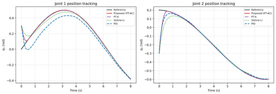
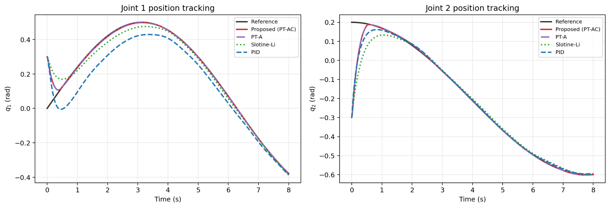
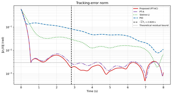
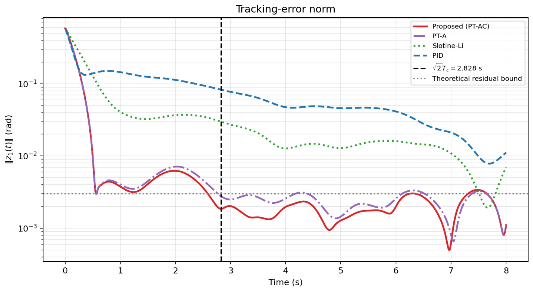
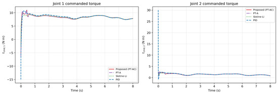
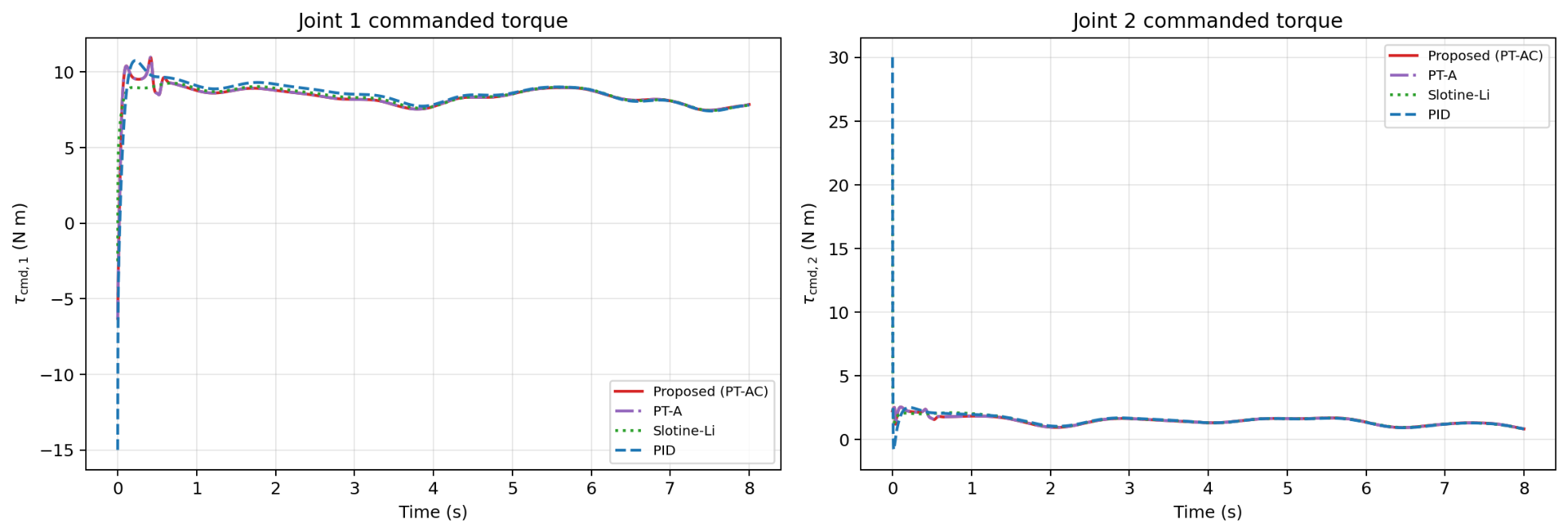
As shown in Figure 1, PT-AC and PT-A exhibit faster position-tracking convergence than Slotine–Li and PID in the nominal case. The corresponding tracking error norms are presented in Figure 2, where both predefined-time controllers achieve rapid error reduction and remain below the practical residual reference level after the transient stage. The vertical line indicates $t=\sqrt{2}{T}_c=2.83$ s, while the horizontal line is included only as a practical reference for numerical visualization rather than as the exact analytical residual bound. As illustrated in Figure 3, PT-AC and PT-A achieve this tracking performance with lower peak commanded torques than Slotine–Li and PID under the nominal simulation conditions.

Figure 1. Nominal Position Tracking.

Figure 2. Nominal Tracking Error Norm.

Figure 3. Unsaturated Commanded Torques.

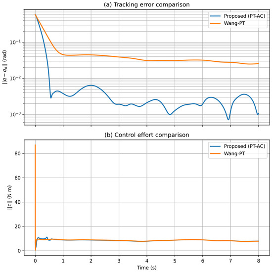
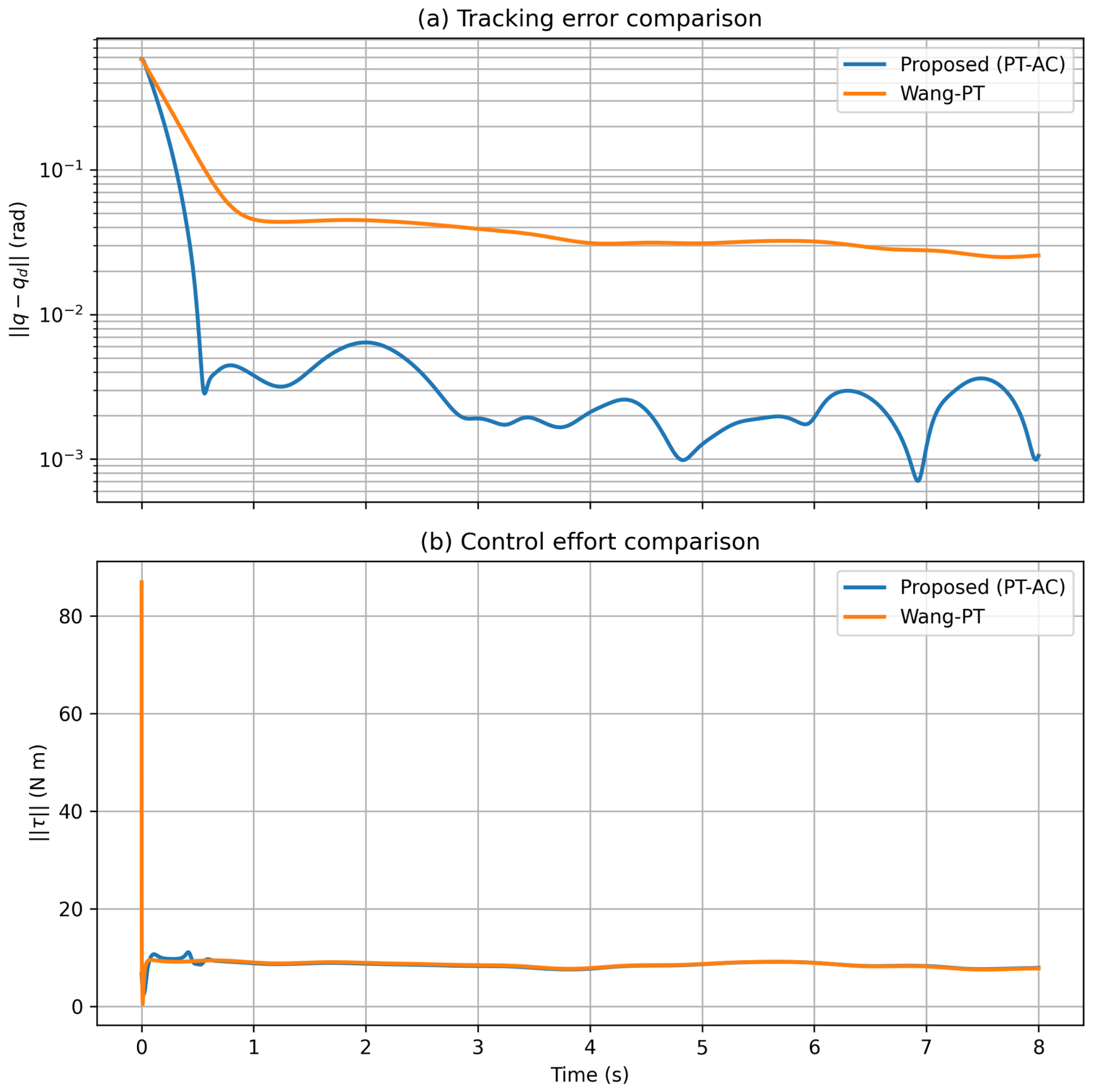
As shown in Figure 4, both predefined-time controllers achieve rapid error reduction. PT-AC obtains smaller post-transient tracking errors while maintaining a comparable control demand. This improvement is attributed to the additional adaptive approximation and critic-modulated learning mechanism, which enhances the compensation of residual modeling uncertainties after the predefined-time transient stage.

Figure 4. External predefined-time baseline comparison between PT-AC and the controller in [3]. (a) Tracking error norm. (b) Commanded control effort.

The quantitative tracking performance is further summarized in Table 1, where the post-transient RMSE is evaluated after $t=\sqrt{2}{T}_c$.

Table 1. Nominal Tracking Performance Comparison.

Controller	${\mathit{T}}_{\mathit{s}}\left(0.05\right)$	RMSEpost	ITAE	${\mathit{\tau }}_{max}$	${\mathit{E}}_{\mathit{\tau }}$
	(s)	(Rad)		(N m)	(N2m2s)
PT-AC	0.3860	0.002015	0.08535	10.97	586.94
PT-A	0.3860	0.002435	0.09801	10.97	587.01
Slotine–Li	0.8565	0.01535	0.53298	23.96	588.58
PID	3.8775	0.04510	1.45958	30.00	611.34

6.4. Adaptive and Learning Signals

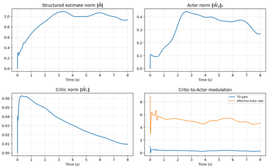
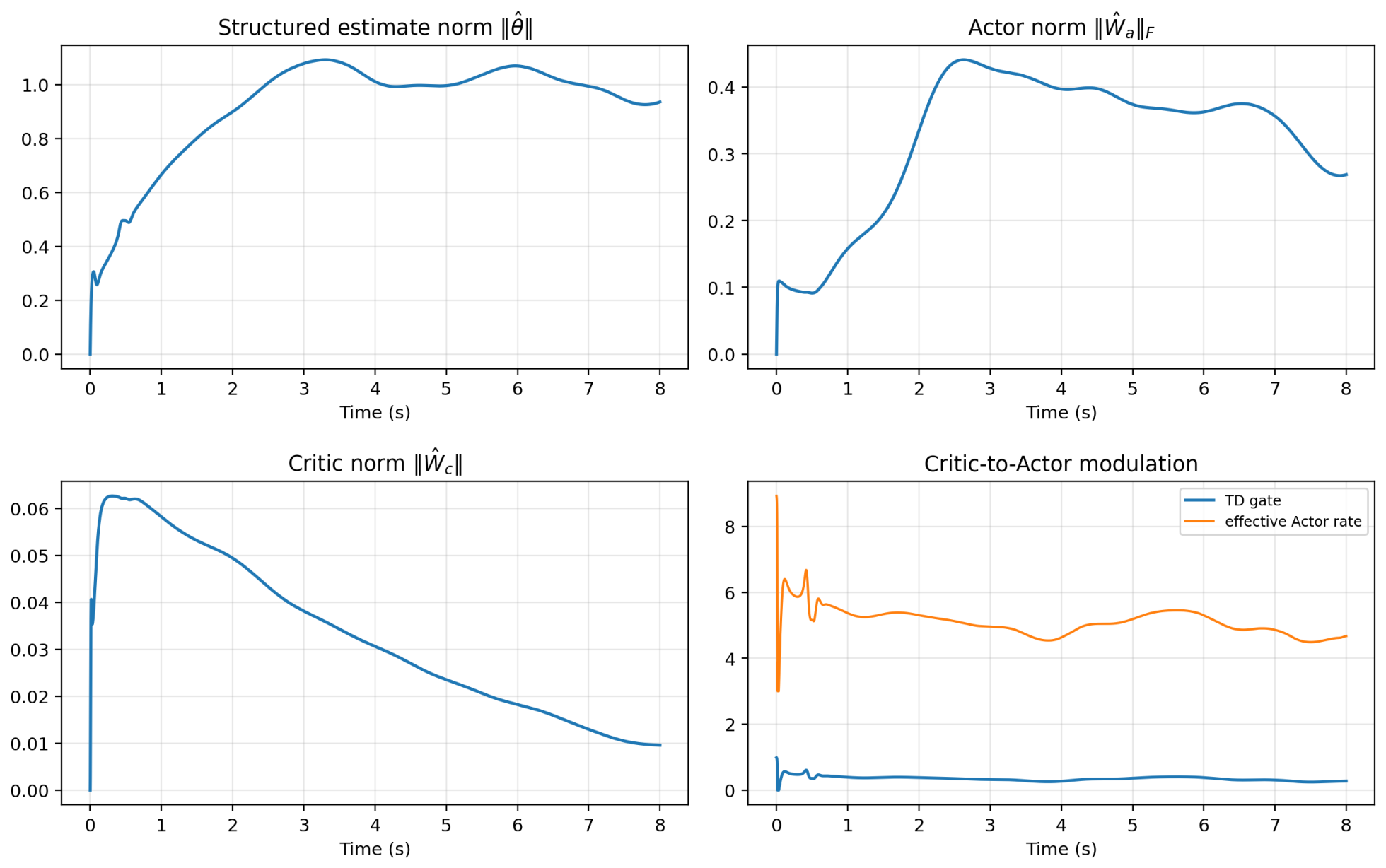
The adaptive trajectories remain bounded throughout the nominal simulation. This numerical observation is consistent with the boundedness properties established in the theoretical analysis. As shown in Figure 5, the structured estimate norm, the actor norm, and the critic norm remain bounded during the nominal simulation, while the bounded TD residual gate and the effective actor learning rate also evolve within bounded ranges. In particular, the bounded critic trajectory observed in Figure 5 is not used as a replacement for the analytical derivation of the critic boundedness condition.

Figure 5. Adaptive and Learning Signals.

6.5. Initial Condition and $T_c$ Studies

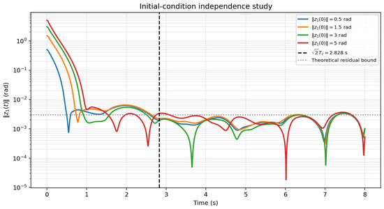
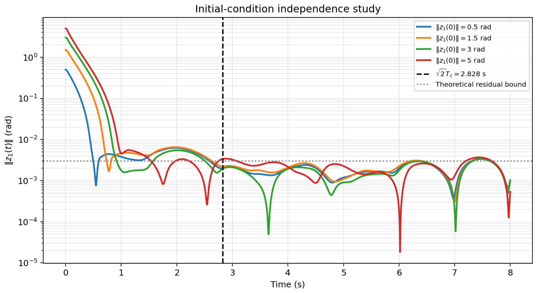
The multi-initial-condition experiment changes only the magnitude of the initial tracking error, while maintaining the same error direction. The results demonstrate that PT-AC preserves a consistent convergence trend over a wide range of initial conditions. A practical residual reference level is included only for visualization and should not be interpreted as the exact analytical residual set.

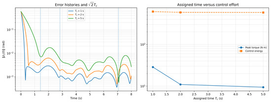
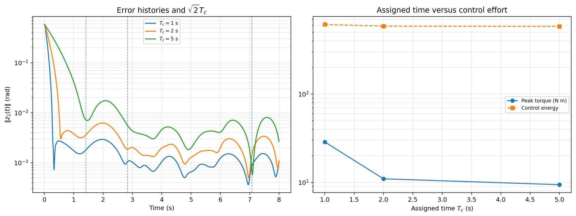
For all tested prescribed-time parameters, $T_c=1$, 2, and 5 s, the empirical permanent entry time remains below $\sqrt{2}{T}_c$. A smaller $T_c$ accelerates the transient response but requires larger control effort, whereas a larger $T_c$ reduces the required command magnitude. The results illustrate the expected convergence–effort trade-off of the predefined-time design.

The multi-initial-condition experiment changes only the magnitude of the initial tracking error, while maintaining the same error direction. As shown in Figure 6, PT-AC preserves a consistent convergence trend over the tested initial conditions, and all trajectories exhibit rapid error reduction relative to the predefined-time reference $t=\sqrt{2}{T}_c$.

Figure 6. Initial-Condition Tracking Performance.

For the prescribed-time parameter study, Table 2 summarizes the empirical settling time, peak commanded torque, and control energy for $T_c=1$, 2, and 5 s. The corresponding trends are illustrated in Figure 7. A smaller $T_c$ accelerates the transient response but requires a larger peak control effort, whereas increasing $T_c$ reduces the required command magnitude and slightly lowers the control energy, illustrating the expected convergence–effort trade-off.

Table 2. $T_c$ sensitivity with all other gains fixed.

${\mathit{T}}_{\mathit{c}}$ (s)	$\sqrt{2}{\mathit{T}}_{\mathit{c}}$ (s)	${\mathit{T}}_{\mathit{s}}\left(0.05\right)$ (s)	${\mathit{\tau }}_{max}$ (N m)	${\mathit{E}}_{\mathit{\tau }}$
1.0	1.414	0.2026	28.67	613.92
2.0	2.828	0.3860	10.97	586.94
5.0	7.071	0.9490	9.42	582.19

Figure 7. Convergence–Effort Trade-Off for Different $T_c$ Values.

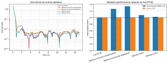
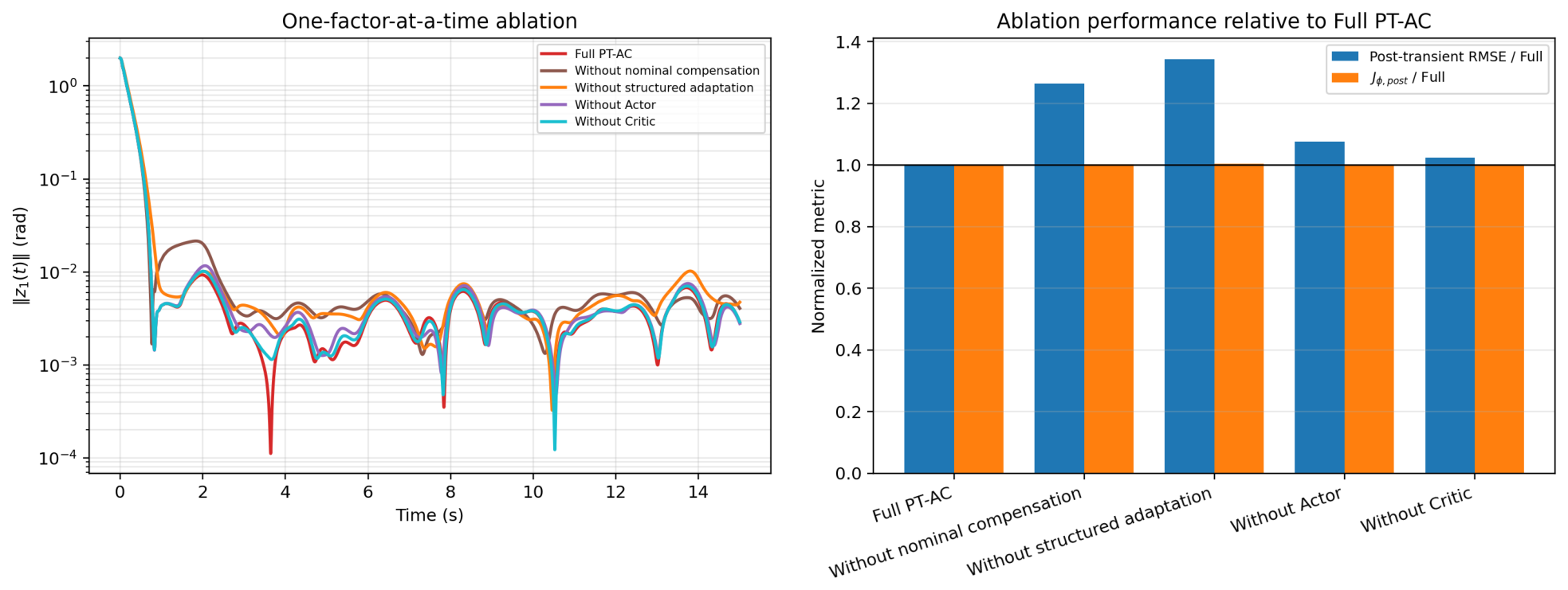
The contribution of the main controller components is further examined in Figure 8. The ablation results indicate that nominal compensation and structured adaptation make the principal contributions to tracking performance, while the actor approximation and critic modulation provide additional refinement of the residual performance.

Figure 8. Component Ablation Study.

6.6. Scope of Numerical Evidence

The numerical studies provide evidence for several aspects of the proposed controller, including predefined-time tracking behavior, residual accuracy, and adaptive boundedness.

The horizontal reference level shown in Figure 2 is introduced as a practical residual reference level for numerical interpretation. It should not be confused with the exact analytical residual set derived in Corollary 1, because the latter depends on explicit Lyapunov constants such as $\overline{\sigma }$ and $c_V$.

The reported simulations therefore distinguish between

• The theoretically established predefined-time and boundedness properties proved in the analysis;
• The practical residual performance observed in numerical experiments.

This separation avoids attributing empirical simulation quantities to unverified analytical constants.

The numerical comparisons demonstrate that PT-AC provides lower post-transient tracking errors than the considered baselines in the tested scenarios while preserving bounded adaptive trajectories and acceptable control effort.

6.7. Discussion

The simulations illustrate the practical tracking performance of PT-AC and are consistent with the theoretical predefined-time and boundedness results. The residual reference level shown in the figures is used only for numerical visualization and should not be interpreted as the analytical residual set, whose value depends on the Lyapunov constants $\overline{\sigma }$ and $c_V$.

Under the considered simulation conditions, PT-AC achieves faster convergence and smaller post-transient tracking errors than Slotine–Li and PID. The ablation results indicate that nominal compensation and structured adaptation make the main contributions to tracking performance, while the actor and critic provide additional residual performance refinement. The comparison with Wang-PT offers an external numerical benchmark but does not establish universal superiority over other predefined-time controllers. The $T_c$ sensitivity study confirms the expected convergence–effort trade-off. The current validation is limited to a 2-DOF manipulator and fixed neural basis functions; experimental validation, higher-dimensional systems, and efficient real-time implementation remain for future investigation.

7. Conclusions

This paper developed an actor–critic predefined-time adaptive tracking controller for partially unknown Euler–Lagrange systems. The implemented torque retains the available nominal rigid-body model and combines structured parameter adaptation, actor-based residual approximation, and continuous robust compensation. The critic modulates the tracking-driven actor update through a bounded squared TD residual gate. The composite Lyapunov analysis establishes the semi-global uniform ultimate boundedness of the closed-loop signals and guarantees that the composite error enters an explicit residual set within $T_P<\sqrt{2}{T}_c$ for initial conditions in the selected compact set.

The retained simulations demonstrate fast nominal tracking, consistent convergence for the tested initial conditions, improved post-transient performance relative to the considered baselines, and the expected convergence–effort trade-off for different prescribed-time parameters. The external predefined-time comparison and component ablation study further support the effectiveness of the proposed architecture under the reported simulation conditions. The current theorem concerns unsaturated state feedback control and does not establish exact policy optimality. Future work will address actuator and state constraints, output feedback learning, experimental validation, and real-time implementation.

References

- Chen, X.; Wang, Y.; Song, Y. Unifying Fixed Time and Prescribed Time Control for Strict-Feedback Nonlinear Systems. IEEE/CAA J. Autom. Sin. 2025, 12, 347–355. [Google Scholar] [CrossRef] [Scilit]
- Yao, Q.; Li, Q.; Jahanshahi, H. Distributed predefined-time neural adaptive control design for consensus of networked Euler-Lagrange systems. Int. J. Syst. Sci. 2024, 56, 1130–1142. [Google Scholar] [CrossRef] [Scilit]
- Wang, W.; Hou, M.; Feng, D.; Liu, B. Predefined-time control for Euler–Lagrange systems with model uncertainties and actuator faults. Asian J. Control 2023, 25, 1591–1605. [Google Scholar] [CrossRef] [Scilit]
- Huang, J.; Zhang, M.; Sun, Y.; Wu, H. Output prediction-based event-triggered interval estimation for continuous-time switched systems. IEEE Trans. Cybern. 2026, early-access. [Google Scholar] [CrossRef] [Scilit] [PubMed]
- Yang, C.; Huang, D.; He, W.; Cheng, L. Neural Control of Robot Manipulators with Trajectory Tracking Constraints and Input Saturation. IEEE Trans. Neural Netw. Learn. Syst. 2021, 32, 4231–4242. [Google Scholar] [CrossRef] [Scilit] [PubMed]
- Bhat, S.P.; Bernstein, D.S. Finite-Time Stability of Continuous Autonomous Systems. SIAM J. Control Optim. 2000, 38, 751–766. [Google Scholar] [CrossRef] [Scilit]
- Polyakov, A. Nonlinear Feedback Design for Fixed-Time Stabilization of Linear Control Systems. IEEE Trans. Autom. Control 2012, 57, 2106–2110. [Google Scholar] [CrossRef] [Scilit]
- Jiménez-Rodríguez, E.; Muñoz-Vázquez, A.J.; Sánchez-Torres, J.D.; Defoort, M.; Loukianov, A.G. A Lyapunov-Like Characterization of Predefined-Time Stability. IEEE Trans. Autom. Control 2020, 65, 4922–4927. [Google Scholar] [CrossRef] [Scilit]
- Pal, A.K.; Kamal, S.; Nagar, S.K.; Bandyopadhyay, B.; Fridman, L. Design of controllers with arbitrary convergence time. Automatica 2020, 112, 108710. [Google Scholar] [CrossRef] [Scilit]
- Sánchez-Torres, J.D.; Gómez-Gutiérrez, D.; López, E.; Loukianov, A.G. A class of predefined-time stable dynamical systems. IMA J. Math. Control Inf. 2018, 35, i1–i29. [Google Scholar] [CrossRef] [Scilit]
- Sánchez Torres, J.D.; Muñoz-Vázquez, A.; Defoort, M.; Aldana-López, R.; Gomez-Gutierrez, D. Predefined-time integral sliding mode control of second-order systems. Int. J. Syst. Sci. 2020, 51, 3425–3435. [Google Scholar] [CrossRef] [Scilit]
- Jiménez-Rodríguez, E.; Sánchez-Torres, J.D.; Gómez-Gutiérrez, D.; Loukianov, A.G. Predefined-time tracking of a class of mechanical systems. In Proceedings of the 2016 13th International Conference on Electrical Engineering, Computing Science and Automatic Control (CCE), Mexico City, Mexico, 26–30 September 2016; pp. 1–5. [Google Scholar] [CrossRef] [Scilit]
- Gao, M.; Ding, L.; Jin, X. ELM-Based Adaptive Faster Fixed-Time Control of Robotic Manipulator Systems. IEEE Trans. Neural Netw. Learn. Syst. 2023, 34, 4646–4658. [Google Scholar] [CrossRef] [Scilit] [PubMed]
- Liu, C.; Li, J.; He, Y.; Jing, A.; Li, L. Neuroadaptive-based fixed-time control for robotic manipulators with uniform prescribed performance under unknown disturbance. Int. J. Robust Nonlinear Control 2024, 34, 10683–10703. [Google Scholar] [CrossRef] [Scilit]
- Xie, Y.; Ma, Q.; Gu, J.; Zhou, G. Event-Triggered Fixed-Time Practical Tracking Control for Flexible-Joint Robot. IEEE Trans. Fuzzy Syst. 2023, 31, 67–76. [Google Scholar] [CrossRef] [Scilit]
- Slotine, J.J.E.; Li, W. On the Adaptive Control of Robot Manipulators. Int. J. Robot. Res. 1987, 6, 49–59. [Google Scholar] [CrossRef] [Scilit]
- Huang, D.; Yang, C.; Pan, Y.; Cheng, L. Composite Learning Enhanced Neural Control for Robot Manipulator with Output Error Constraints. IEEE Trans. Ind. Inform. 2021, 17, 209–218. [Google Scholar] [CrossRef] [Scilit]
- Sun, Y.; Yan, B.; Shi, P.; Lim, C.C. Consensus for Multiagent Systems Under Output Constraints and Unknown Control Directions. IEEE Syst. J. 2023, 17, 1035–1044. [Google Scholar] [CrossRef] [Scilit]
- Zhang, Y.; Hua, C. Composite Learning Finite-Time Control of Robotic Systems with Output Constraints. IEEE Trans. Ind. Electron. 2023, 70, 1687–1695. [Google Scholar] [CrossRef] [Scilit]
- Sun, Y.; Shi, P.; Lim, C.C. Adaptive consensus control for output-constrained nonlinear multi-agent systems with actuator faults. J. Frankl. Inst. 2022, 359, 4216–4232. [Google Scholar] [CrossRef] [Scilit]
- Ai, Z.; Wang, H. Adaptive predefined-time tracking control of nonlinear systems with unmodeled dynamics. Int. J. Control 2025, 98, 2709–2718. [Google Scholar] [CrossRef] [Scilit]
- Doya, K. Reinforcement Learning in Continuous Time and Space. Neural Comput. 2000, 12, 219–245. [Google Scholar] [CrossRef] [Scilit] [PubMed]
- Al-Tamimi, A.; Lewis, F.L.; Abu-Khalaf, M. Model-free Q-learning designs for discrete-time zero-sum games with application to H-infinity control. In Proceedings of the 2007 European Control Conference (ECC), Kos, Greece, 2–5 July 2007; pp. 1668–1675. [Google Scholar] [CrossRef] [Scilit]
- Zhao, X.; Tao, B.; Qian, L.; Ding, H. Model-Based Actor-Critic Learning for Optimal Tracking Control of Robots with Input Saturation. IEEE Trans. Ind. Electron. 2021, 68, 5046–5056. [Google Scholar] [CrossRef] [Scilit]
- Rahimi Nohooji, H.; Zaraki, A.; Voos, H. Actor–critic learning based PID control for robotic manipulators. Appl. Soft Comput. 2024, 151, 111153. [Google Scholar] [CrossRef] [Scilit]
- Tam, L.T.M.; Ngu, N.V.; Pham, D.H.; Mai, V.T. Disturbance Observer-Based Actor–Critic Reinforcement Learning with Adaptive Reward for Energy-Efficient Control of Robotic Manipulators. Actuators 2026, 15, 167. [Google Scholar] [CrossRef] [Scilit]
Disclaimer/Publisher’s Note: The statements, opinions and data contained in all publications are solely those of the individual author(s) and contributor(s) and not of MDPI and/or the editor(s). MDPI and/or the editor(s) disclaim responsibility for any injury to people or property resulting from any ideas, methods, instructions or products referred to in the content. |
© 2026 by the authors. Licensee MDPI, Basel, Switzerland. This article is an open access article distributed under the terms and conditions of the Creative Commons Attribution (CC BY) license.