Friction Compensation Method Based on a Dual-Segment Simplified Static–Dynamic Friction Model

Abstract

Nonlinear friction in the mechanical transmission system of machine tools induces transient stagnation of the feed axis as its velocity crosses zero, thereby giving rise to contouring errors in multi-axis machining and significantly degrading machining accuracy. To address this issue, a feedforward compensation strategy is proposed based on a simplified static friction model (SSFM) with dual-segment and dual-parameter characteristics. The nonlinear friction is represented by a combination of a linear segment and an exponential segment, while the model incorporates two essential parameters that characterize the maximum friction force and the negative damping effect. Experimental results from two-axis circular trajectory tests show that the proposed SSFM reduces contour errors by approximately 73.4% and 79.2% at 600 mm/min and 2100 mm/min, respectively. To improve compensation under high-speed conditions, an acceleration-dependent dynamic correction is further introduced to establish the SDFM. The results show that the maximum contour error is further reduced to 1.44 μm and 1.49 μm at 3600 mm/min and 5000 mm/min, respectively. Compared with many existing reduced-order or hybrid friction models that rely on more parameters or more complex identification procedures, the proposed method provides a more compact and compensation-oriented modeling strategy for the velocity-reversal region of CNC feed systems.

1. Introduction

During the operation of the servo feed system in machine tools, especially when the motion direction changes, nonlinear friction can cause transient stick–slip stagnation of the feed system. This leads to phenomena such as velocity zero-crossing, position flat-topping, and quadrant sharp-corner distortions in circular interpolation. These adverse effects induced by nonlinear friction degrade the machining accuracy of CNC machine tools. To reduce the negative impact of nonlinear friction on the control performance of servo systems during multi-axis coordinated machining, numerous scholars have carried out extensive research on friction compensation methods. At present, compensation methods for nonlinear friction can be broadly categorized into two groups: non-model-based approaches [1,2,3,4,5,6,7,8] and model-based approaches [9].

Non-model-based compensation methods regard friction as an external disturbance to the system and enhance the system’s robustness against such disturbances by optimizing the control structure, adjusting control parameters, or applying additional external signals. This category of compensation methods includes PID control, robust control, pulse control, and various advanced control strategies [10,11,12]. Such approaches avoid the modeling and parameter identification processes of friction models, and are therefore relatively simple to implement. However, these methods exhibit certain limitations. For instance, when employing PID control, it is difficult to eliminate the creeping phenomenon caused by nonlinear friction during motion reversals. In pulse compensation, determining parameters such as pulse width, amplitude, and insertion timing is highly challenging. Non-model-based compensation methods based on advanced control strategies also face obstacles in practical engineering applications. For example, neural network-based approaches often suffer from long training times and poor stability; fuzzy control requires difficult-to-obtain rule sets and involves excessive computation when the number of inputs increases; and sliding mode control tends to generate high-frequency chattering, which deteriorates machining accuracy. Taken together, these limitations indicate that non-model-based compensation methods are constrained by multiple factors, and their compensation performance often falls short of expectations.

Model-based compensation methods require the establishment of a mathematical model of the friction component and the identification of its parameters. The resulting friction model is then incorporated into the feedforward compensation framework of the control system to mitigate the adverse effects induced by nonlinear friction. In general, the effectiveness of model-based compensation strongly depends on the construction of an accurate nonlinear friction model. In previous studies, various mathematical formulations of friction have been proposed, which can generally be classified into static models and dynamic models [13]. With the continuous refinement of nonlinear friction modeling and the introduction of improved modeling techniques, the compensation capability of model-based methods has been significantly enhanced, making them one of the mainstream directions in friction compensation research. Existing studies have shown that model-based methods can improve compensation performance from different perspectives. For example, Liu et al. [14] introduced an inertia term of the joint driving force into the traditional Stribeck model as a thrust component, thereby accounting for inertia variations in the compensation process. Feng et al. [15] employed an improved LuGre friction model to capture friction characteristics associated with position, velocity, and motion direction. Wan et al. [16] used a continuously differentiable dual-arctangent curve to construct a dynamic friction model that effectively described the asymmetric nonlinear friction characteristics of machine tools in positive and negative velocity regions. Wang et al. [17] proposed a fuzzy low-pass-filter-based compensation approach derived from the Stribeck model to enhance robustness over a wide velocity range. Dai et al. [18] developed an improved LuGre friction model for electro-hydrostatic force servo systems to represent friction asymmetry in opposite velocity intervals and to reduce force impact during compensation. Han et al. [19] introduced a time-delay neural network to model the nonlinear friction of hydraulic actuators, while Huang et al. [20] proposed a hybrid LuGre-Net model combining the LuGre model with neural networks to improve friction prediction accuracy. Jiang et al. [21] developed an adaptive compensation scheme based on the LuGre model to enhance system stability.

Although these studies demonstrate that model-based methods are capable of improving friction compensation accuracy, they also reveal several limitations. First, many of the existing approaches achieve better compensation performance by introducing additional nonlinear terms, internal state variables, adaptive mechanisms, or data-driven structures, which improves descriptive capability but also increases model complexity. Second, the associated parameter identification process is often nontrivial, especially for models with multiple coupled parameters, and may require extensive experiments, optimization procedures, or training data support. Third, some advanced models are developed for broader dynamic friction reconstruction, but their complexity may exceed the practical requirements of real-time compensation in CNC feed systems, where implementation simplicity and computational efficiency are also important considerations. Therefore, the main difficulty of model-based friction compensation lies not only in improving modeling accuracy, but also in achieving a reasonable balance among model fidelity, parameter identification effort, and engineering implementability. In practice, many friction models with good compensation performance still involve a relatively large number of parameters, and the identification process is often complex and time-consuming. These factors limit the practical applicability of model-based friction compensation methods in actual CNC systems. From this perspective, a simplified friction model that preserves the dominant friction characteristics in the velocity-reversal region while reducing parameter complexity remains of clear practical significance.

Currently, research on friction model-based compensation methods primarily focuses on two aspects: the construction of friction models and the accurate identification of model parameters. However, relatively comprehensive friction models, such as the LuGre model, usually involve multiple parameters to be identified (e.g., seven parameters), and the identification process is often complex and difficult to implement in engineering practice, which limits the application of such methods in actual CNC systems. To address these issues, this paper simplifies the nonlinear friction effect curve in a control-oriented manner and develops a Simplified Static Friction Model (SSFM) and a Simplified Dynamic Friction Model (SDFM). Although a number of simplified friction models have been reported in the literature, the contribution of this study is not limited to parameter reduction. Instead, the proposed method establishes a reduced-order friction compensation framework for the velocity-reversal region of CNC feed systems, where contour errors are most sensitive to friction nonlinearity. In the proposed SSFM, the dominant friction behavior in this region is described by a linear segment and an exponential segment, corresponding to the presliding deformation stage and the Stribeck transition stage, respectively. Based on this structure, the SDFM further introduces an acceleration-dependent correction to improve compensation performance under high-speed reversal conditions.

Compared with the LuGre model, the proposed models contain only two to three parameters, which can be determined by an engineering trial-and-error procedure, thereby reducing the complexity of parameter tuning and improving practical implementability. Experimental results show that, compared with the SSFM, the proposed SDFM not only maintains satisfactory friction compensation performance under low-speed conditions but also achieves better compensation performance under high-speed conditions, thereby alleviating the degradation of static friction compensation during high-speed operation. Therefore, the main contribution of this work lies in providing a control-oriented simplified modeling approach that achieves a practical balance among model compactness, compensation effectiveness, and real-time implementability.

It should be noted that the present study mainly focuses on model structure simplification and improvement of parameter determination efficiency. The proposed models remain simplified forms without introducing internal state variables and therefore have certain limitations in describing complex dynamic friction behaviors, such as stick–slip effects at very low speeds. Future work will further extend the model to improve its capability in characterizing more complex dynamic friction phenomena. The remainder of this paper is organized as follows. Section 2 presents the design and experimental validation of the SSFM. Section 3 introduces the design and experimental validation of the SDFM. Section 4 concludes the paper.

2. Design and Experimental Validation of the SSFM

2.1. Design of the SSFM

Friction models can generally be divided into two categories. The first is static friction models, such as the Coulomb model, viscous friction model, Stribeck model, and Karnopp model. The second is dynamic friction models, such as the Dahl model and the LuGre model. Among them, the LuGre model distinguishes between two states of friction, namely presliding and sliding, and achieves a smooth transition between these states through a nonlinear differential equation. As a result, the LuGre model is capable of accurately characterizing nonlinear friction phenomena. The mathematical formulation of the LuGre model is expressed as shown in Equation (1):

$$F(v)=\left\{\begin{array}{l}g\left(v\right)=F_C+\left(F_S-F_C\right)e^{-{\left({\displaystyle \frac{v}{v_s}}\right)}^2}\\ \dot{z}=v-{\displaystyle \frac{{\sigma }_0}{g\left(v\right)}}\cdot \left|v\right|\\ F={\sigma }_{0}z+{\sigma }_1\dot{z}+{\sigma }_{2}v\end{array}\right.$$

(1)

In Equation (1), F_S denotes the maximum static friction force, F_C is the Coulomb friction force, v_s is the Stribeck velocity, σ₀ is the bristle stiffness coefficient, σ₁ is the bristle damping coefficient, σ₂ is the viscous friction coefficient, and z is the bristle elastic deformation. As can be seen from the mathematical formulation of the LuGre model, friction compensation based on this model requires the identification of seven parameters, making the identification process complex and challenging. To reduce the difficulty of parameter identification while maintaining effective friction compensation, this study simplifies the nonlinear stage of friction and develops an SSFM.

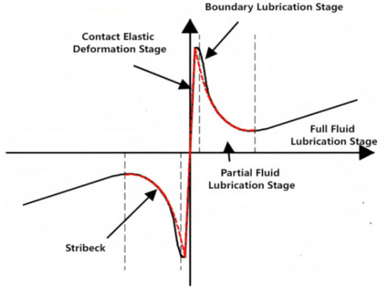
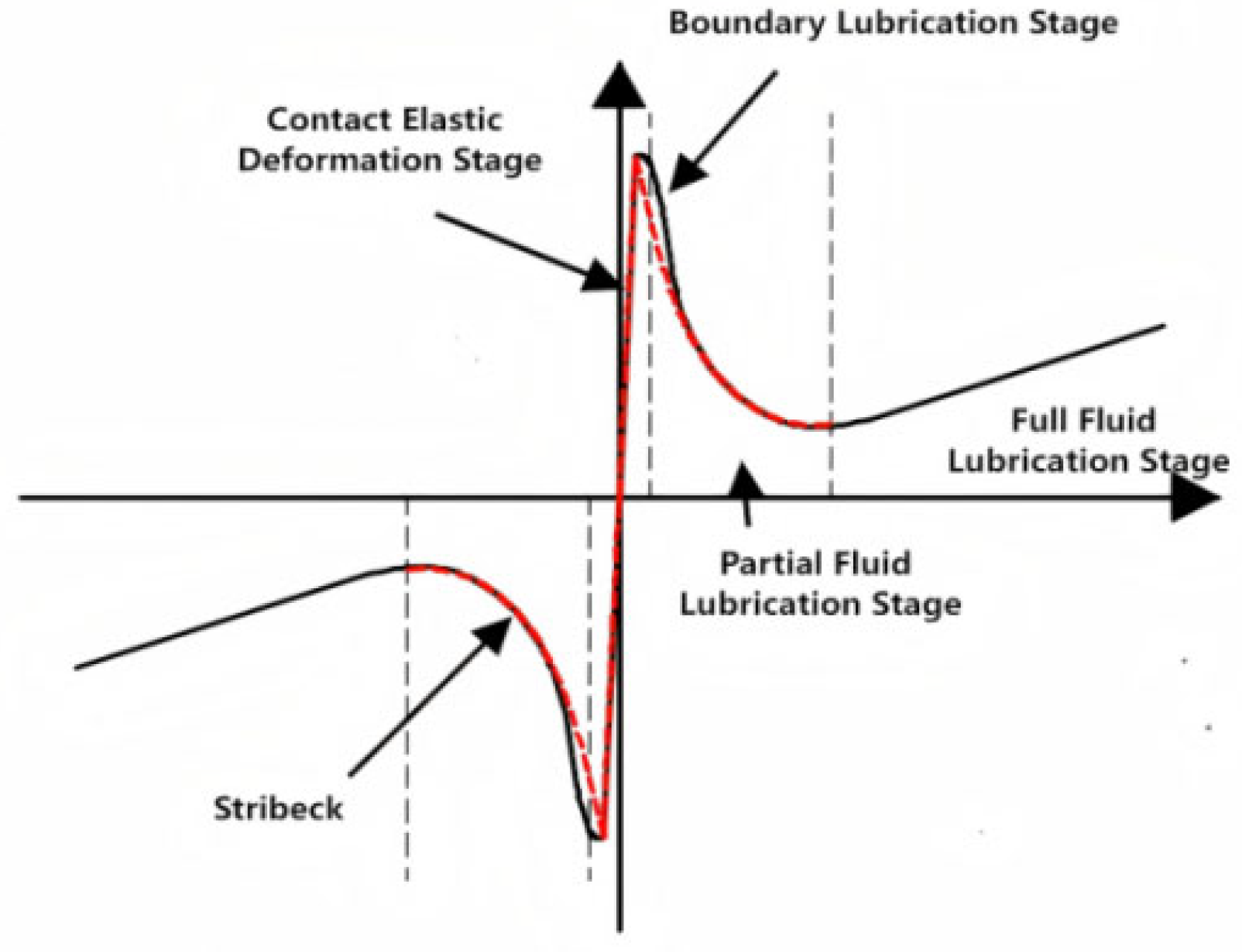
As shown in Figure 1, the black solid line represents the nonlinear friction effect curve. Through an analysis of the frictional effects at different stages, it is observed that the nonlinear behavior of friction mainly occurs during the contact elastic deformation stage, the boundary lubrication stage, and a portion of the fluid lubrication stage. To meet the accuracy requirements of friction compensation, these three stages are simplified into two segments: a linear function stage and an exponential function stage. The red dashed line in Figure 1 illustrates the friction effect curve after simplification, which serves as the basis for designing the SSFM.

Figure 1. Nonlinear Friction Effect Curve.

The linear function stage is defined as follows: during the contact elastic deformation stage, the friction force is primarily caused by the elastic deformation between the contact surfaces. In this case, the friction force exhibits an approximately linear relationship with the displacement in the presliding stage:

$$F_{f1}=k\cdot x_1\begin{array}{cc}& x_1\end{array}\le \alpha ,F_{f1}\le F_f$$

(2)

In Equation (2), F_f1 denotes the equivalent linear-stage friction force (with F_f representing the maximum friction force in the equivalent linear stage), k is the stiffness coefficient of the equivalent linear stage, and x₁ denotes the displacement in the equivalent linear presliding stage (with α representing the maximum displacement in the presliding stage, which is typically taken as an empirical constant of 4 µm).

Within the short duration of machine tool reversal, the system response can be approximated as a uniformly accelerated process, and x₁ can thus be expressed as:

$$x_1={\displaystyle \frac{1}{2}}a{t}^2={\displaystyle \frac{1}{2}}vt\begin{array}{cc}& v\end{array}\le v_1$$

(3)

In Equation (3), t represents the motion time, a the actual acceleration, and v the actual velocity. Here, v₁ denotes the critical velocity at which the system transitions from the boundary lubrication stage and the contact elastic deformation stage to the partial fluid lubrication stage, and v = v₁ corresponds to the time instant at which the maximum presliding displacement α is reached.

By combining Equations (2) and (3), the equivalent linear friction model for the boundary lubrication stage and the contact elastic deformation stage can be obtained, as expressed in Equation (4):

$$F_{f1}={\displaystyle \frac{vt}{2\alpha }}\cdot F_f\begin{array}{cc}& v\end{array}\le v_1$$

(4)

The exponential function stage is defined as follows: in the fluid lubrication stage, the nonlinear friction force is primarily characterized by the “Stribeck effect,” which can be described by the Stribeck mathematical model as shown in Equation (5):

$$F(v)=\left[F_C+\left(F_S-F_C\right)e^{-{\left({\displaystyle \frac{v}{v_s}}\right)}^{\delta }}\right]\mathrm{sgn}\left(v\right)+{\sigma }_{2}v$$

(5)

In Equation (5), F_S represents the maximum static friction force, F_C the Coulomb friction force, v_s the Stribeck velocity, σ₂ the viscous friction coefficient, and δ an empirical constant. As shown by Equation (5) and Figure 1, in the “Stribeck effect” stage, the relationship between friction force and velocity exhibits an approximately exponential trend. Therefore, to more effectively describe the friction–velocity relationship in the fluid lubrication stage, this process is equivalently approximated by an exponential function.

$$F_{f2}=F_f\cdot {\left({\displaystyle \frac{v}{v_2}}\right)}^{-\varphi }{\begin{array}{cc}& v\end{array}}_2\le v<v_s$$

(6)

where Φ is the friction compensation coefficient in the exponential-stage function.

By combining Equations (4) and (6), the simplified friction model for the nonlinear stage of the servo feed system during velocity reversal can be obtained, and its mathematical expression is given as:

$$\left\{\begin{array}{l}{F}_{f1}={\displaystyle \frac{vt}{2\alpha }}\cdot \Delta e\begin{array}{cc}\begin{array}{cc}& \end{array}& v\le v_1\end{array}\hfill \\ F_{f2}=\Delta e\cdot {\left({\displaystyle \frac{v}{v_2}}\right)}^{-\varphi }{\begin{array}{cc}& v\end{array}}_2\le v<v_s\hfill \end{array}\right.$$

(7)

where Δe is the friction compensation amount. Based on Equation (7), when the velocities are equal (v₁ = v₂), the contact elastic deformation stage begins to transition into the partial fluid lubrication stage. In the simplified friction model, this corresponds to the transition from the linear function segment to the exponential function segment. At this critical velocity, x₁ reaches the maximum presliding displacement, i.e.,

$${\displaystyle \frac{vt}{2}}=a$$

(8)

At this point, the outputs of the linear and exponential segments can be expressed as follows:

$$\left\{\begin{array}{l}{F}_{f1}=\Delta e\hfill \\ F_{f2}=\Delta e\hfill \end{array}\right.$$

(9)

According to Equation (9), the outputs of the linear and exponential segments are equal at the critical velocity, which indicates that the model is continuous at the switching point. This continuity makes the transition relatively smooth and ensures stable and continuous variation in the friction force.

To verify the validity of the SSFM, an approximation error analysis is carried out. Let F_L(v) denote the friction force described by the original LuGre-type nonlinear model in the velocity reversal region, and let F_SS(v) denote the friction force generated by the proposed SSFM. The modeling error is defined as

$$e(v)=F_L(v)-F_{\mathit{SS}}(v)$$

(10)

In the presliding region, where the relative velocity is sufficiently small, the friction law can be locally expanded by Taylor series around v = 0. Since the friction–displacement relation is smooth in a sufficiently small neighborhood of zero velocity, the LuGre friction law can be approximated by its first-order term:

$$F_L(v)=F_L(0)+{\displaystyle \frac{dFL}{dv}}{|}_{v=0}+o(v^2)$$

(11)

The linear segment of the SSFM corresponds to retaining the dominant first-order term. Therefore, the local approximation error in this region satisfies

$$e(v)=o(v^2),v\to 0$$

(12)

This indicates that the proposed linear segment is theoretically reasonable in the neighborhood of velocity reversal, where the friction-induced contour error is most critical.

In the Stribeck transition region, the nonlinear friction curve is dominated by an exponentially decaying trend. The exponential segment adopted in the SSFM preserves the principal shape of the original friction law. Let F_E(v) denote the exponential approximation in this interval. If the characteristic velocity and peak friction are matched at the transition point, then the residual approximation error mainly depends on higher-order curvature mismatch, that is,

$$e(v)=F_L(v)-F_E(v)=o({\left(v-v_c\right)}^2)$$

(13)

in a local neighborhood of the switching velocity v_c. Hence, the dual-segment SSFM provides a second-order local approximation accuracy near the matching point.

From the control viewpoint, the resulting tracking improvement depends not only on the absolute modeling error, but also on whether the compensation model captures the dominant friction variation near reversal. Since the largest contour error is produced by friction nonlinearity in the low-velocity interval, the proposed SSFM remains effective even though it is a reduced-order approximation. This explains why the model can achieve significant error reduction with only two key tunable parameters.

2.2. Description of the Experimental Platform

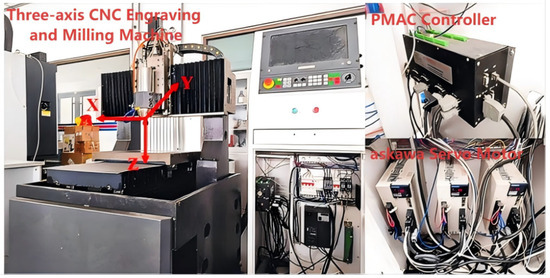
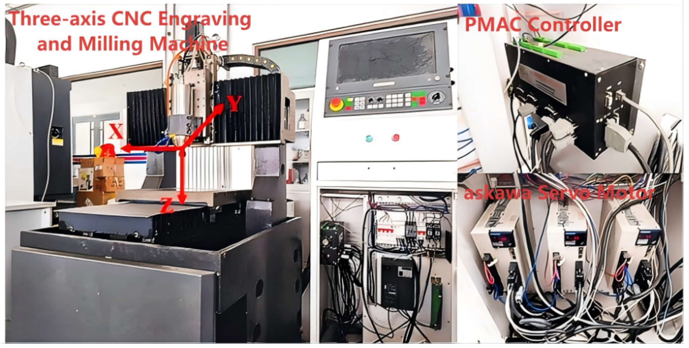
This study was carried out on a three-axis engraving and milling machine experimental platform, as shown in Figure 2. The controller executes the servo control algorithm digitally, while the driver operates in torque control mode. The feedback signal of the motion controller is provided by the encoder of the servo motor, and the sampling time is 0.00408 s, thereby forming a semi-closed-loop control system. This configuration enables the machine to maintain stable motion and positioning accuracy even under varying load conditions. The controller used in this study is a PAMC motion controller manufactured by Delta Tau Data Systems, Chatsworth, CA, USA. This controller is a widely applied programmable multi-axis motion control card that supports numerous functions. It is capable of handling various tasks required for mechanical control, including executing motion programs, running PLC programs, updating servo loops, performing commutation updates, and communicating with the host computer.

Figure 2. Three-Axis Engraving and Milling Machine Experimental Platform.

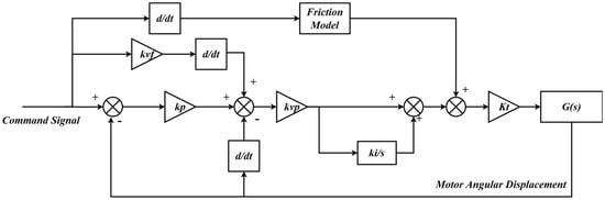
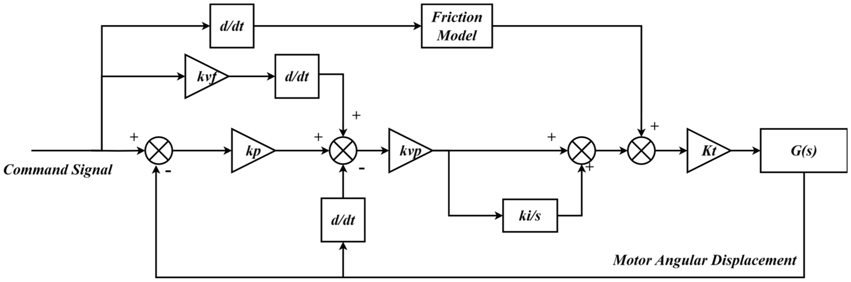
The servo system of the experimental platform adopts a PID triple closed-loop control structure, as shown in Figure 3. The current loop is embedded within the servo driver and is only related to the internal parameter settings of the driver; therefore, only the position loop and the velocity loop are illustrated in the control structure diagram. In the figure, kp and kvp represent the gain coefficients of the position loop and the velocity loop, respectively; ki denotes the integral gain coefficient; Kt is the torque coefficient; kvf represents the velocity feedforward coefficient. G(s) is the transfer function of the mechanical component of the test bench, and the friction model represents the designed simplified friction model.

Figure 3. Servo System Control Framework.

2.3. Experimental Validation of the SSFM

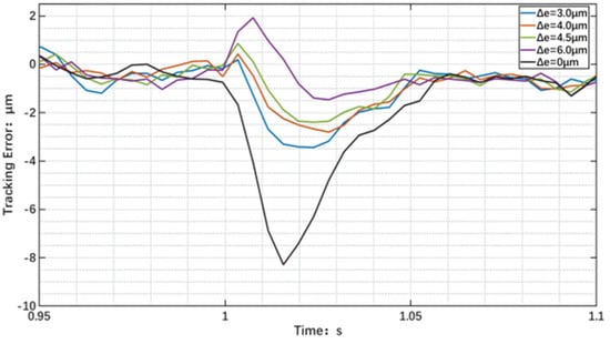
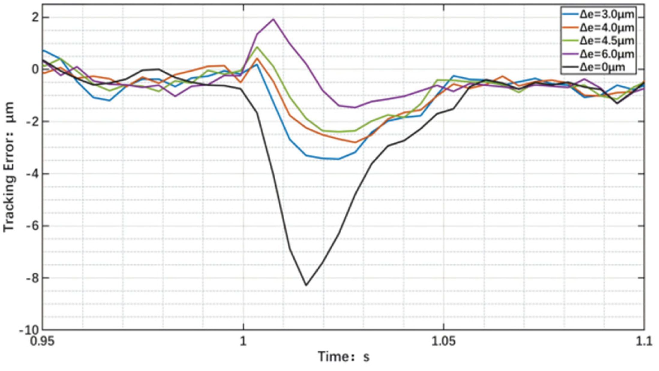
To verify the effectiveness of the proposed friction compensation method based on the SSFM, the compensation algorithm was implemented in the servo control system, and an X-axis friction feedforward compensation experiment was carried out. The simplified friction model includes two tunable parameters: the compensation term Δe and the compensation coefficient Φ. In the experiment, the displacement of the X-axis cosine input signal was set to 50 mm with a motion time of 2 s, and the compensation coefficient Φ was fixed at 1. By gradually adjusting the value of the compensation term Δe, variation in tracking error under different compensation values Δe was observed, and the optimal compensation value was thereby determined, as shown in Figure 4.

Figure 4. The Effect of Compensation Term Δe Variation on Friction Compensation.

The compensation term Δe plays a key role in determining the magnitude of friction feedforward compensation in the reversal region. Physically, it can be interpreted as an equivalent compensation quantity used to offset the displacement loss and tracking lag caused by nonlinear friction near zero velocity. When Δe is selected too small, the actual friction effect cannot be sufficiently compensated, and the feed axis still exhibits an evident tracking error after reversal. As Δe gradually increases, the compensation action becomes stronger, and the friction-induced reversal error is correspondingly reduced.

However, the improvement is not monotonic without limitation. If Δe is excessively large, the applied compensation exceeds the actual friction demand at the initial stage of reversal, so that the feed axis may respond too early or too strongly, leading to overcompensation. This is reflected in the experimental results as a transient error in the opposite direction near the reversal point. Therefore, the compensation term Δe should be selected within a suitable range so as to balance insufficient compensation and excessive compensation. Based on the experimental comparison, Δe = 4.5 μm was found to provide the best overall compensation effect in this study.

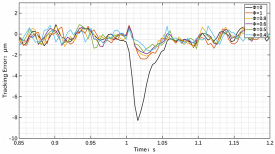
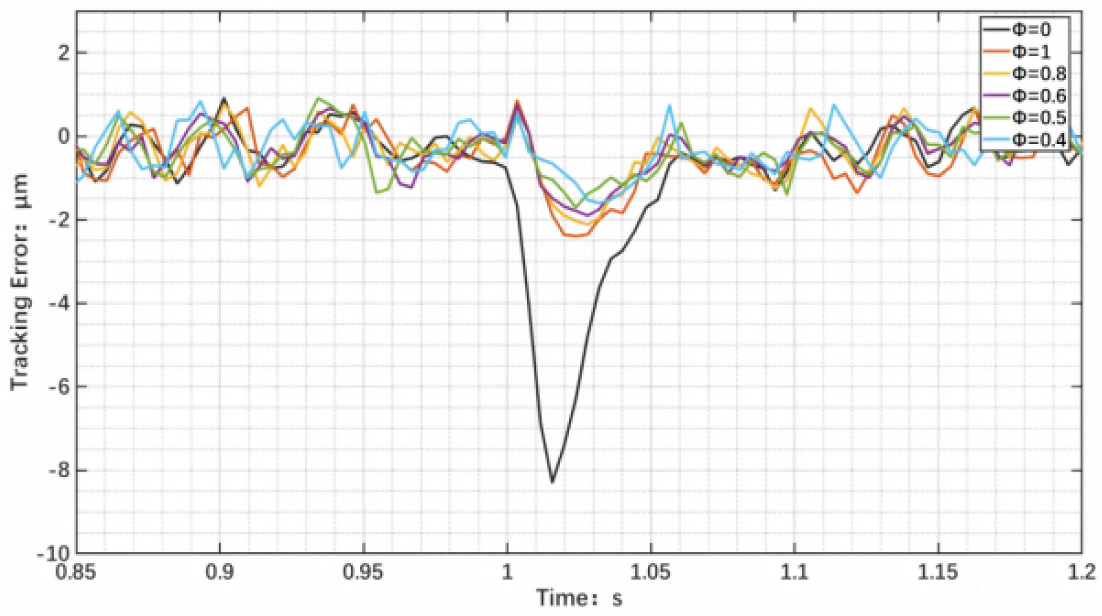
According to the experimental results shown in Figure 5, as the compensation coefficient Φ decreases, both the initial overcompensation at the reversal stage and the tracking error during reversal tend to diminish. However, when Φ is set too small, an overcompensation phenomenon appears at the end of the trajectory, which adversely affects the overall friction compensation performance. Taking into account both the compensation effectiveness and the occurrence of overcompensation, the optimal parameters were determined as a compensation value Δe = 4.5 μm and a compensation coefficient Φ = 0.6.

Figure 5. The Effect of Compensation Coefficient Φ Variation on Friction Compensation.

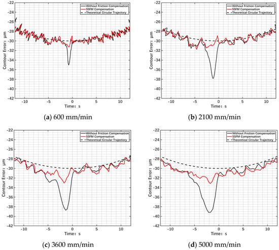
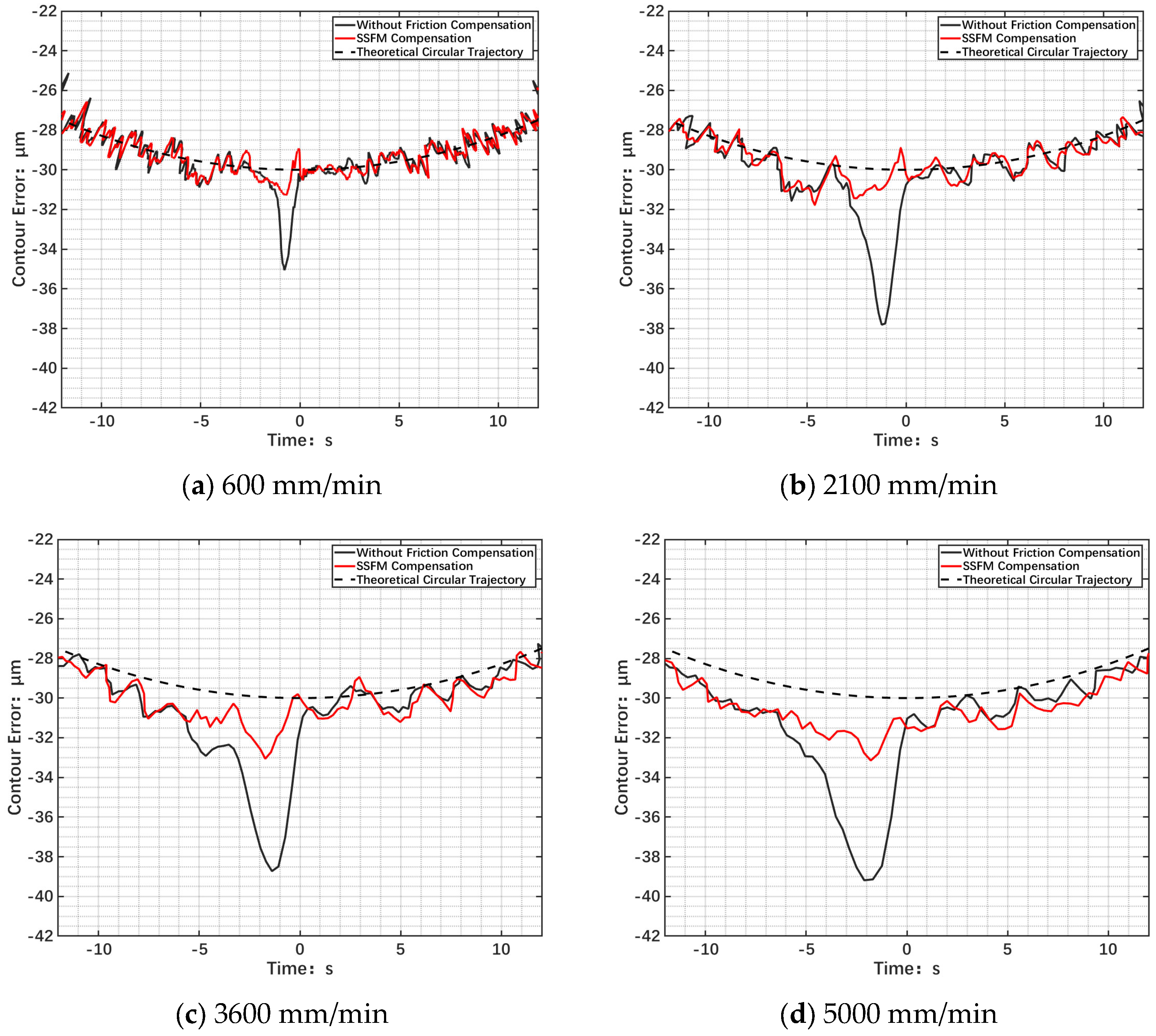
After determining the values of the compensation term Δe and the compensation coefficient Φ, the performance of the simplified static model under different velocity conditions was evaluated. The feed rates were set to 600 mm/min, 2100 mm/min, 3600 mm/min, and 5000 mm/min, respectively, and a two-axis circular interpolation trajectory tracking experiment was conducted with a radius of R = 30 mm. To make the trajectory error more clearly visible in the figure, the trajectory radius was set to (R−29.970) mm, and the experimental contour error diagram was obtained. The experimental results are presented in Figure 6.

Figure 6. Contour Error Compensation Using the SSFM.

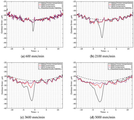
Figure 6 illustrates the contour error results of the friction compensation experiments based on the SSFM under different velocity conditions. The data indicate that, after compensation with the SSFM, the motion control performance of the system is significantly improved. Under the velocity condition of 600 mm/min, after compensation with the static friction model, the maximum contour error of the feed axis was reduced from 5.07 μm to 1.35 μm, a reduction of approximately 73.4%. When the velocity reached 2100 mm/min, the maximum contour error of the feed axis decreased from 7.75 μm to 1.61 μm, corresponding to a reduction of about 79.2%. However, when the machine operating speed was further increased to 3600 mm/min and 5000 mm/min, significant contour errors still occurred in the feed axis during reversal. After compensation, the maximum contour errors of the feed axis were 3.05 μm and 3.21 μm, respectively, indicating that the compensation effect of the static friction model was unsatisfactory under high-speed conditions.

In summary, the proposed simplified friction model demonstrates good compensation performance under low-speed conditions, but significant contour errors remain at high speeds, and the compensation effect deteriorates. This is because nonlinear friction exhibits complex dynamic characteristics, with its behavior varying under different motion states. The SSFM, however, cannot account for these dynamic characteristics, which leads to poor compensation performance during reversals at high operating speeds. Since the acceleration of the feed system differs across velocity reversal processes, it is necessary to investigate the variation in friction under different acceleration conditions. Accordingly, the SSFM should be extended to a dynamic model in order to enhance the compensation capability.

3. Design and Experimental Validation of the SDFM

3.1. Design of the SDFM

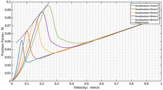
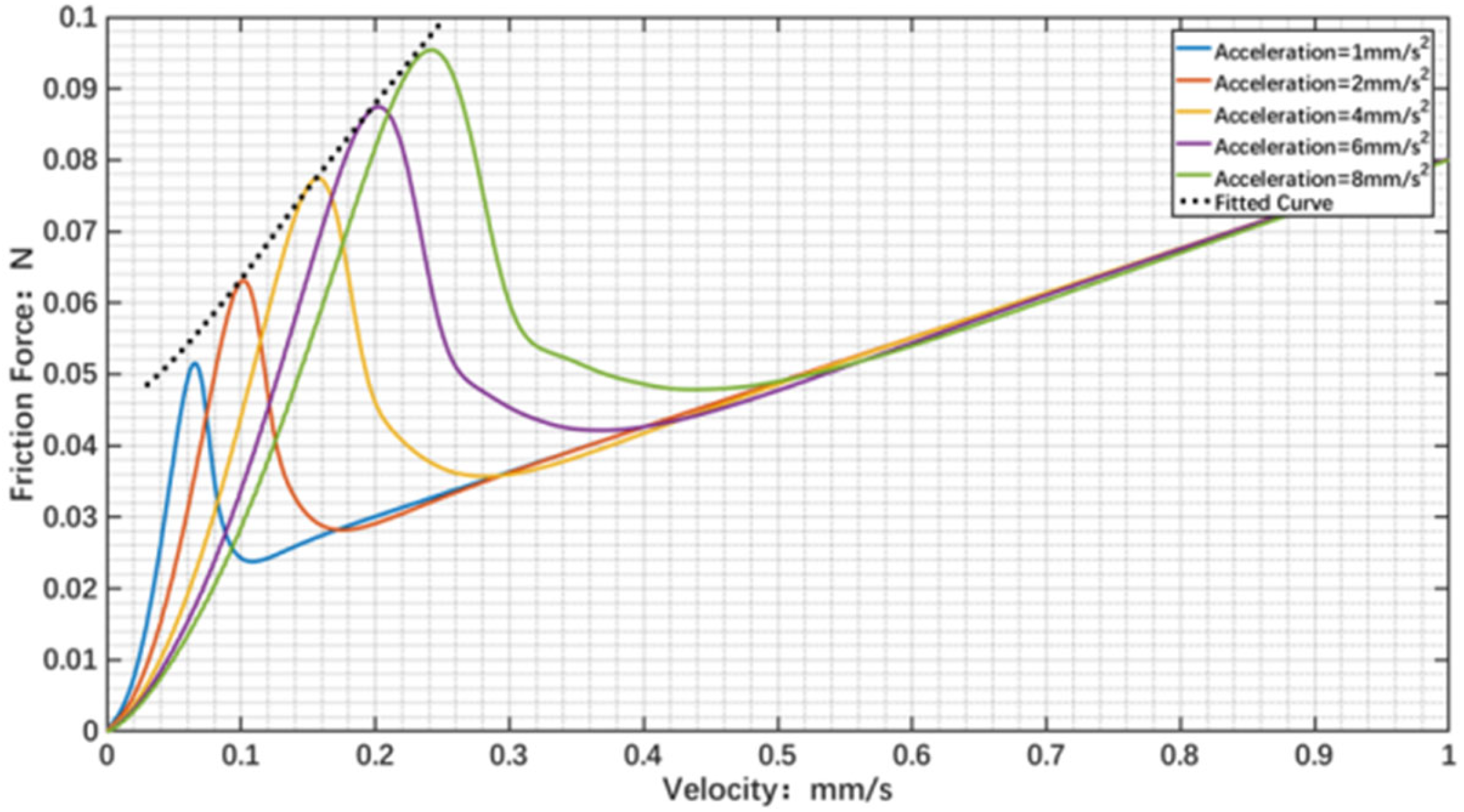
To investigate the variation in nonlinear friction under different acceleration operating conditions of the machine tool feed system, the LuGre model was adopted to represent the system friction force. By applying velocity signals with different accelerations to the control system for simulation, the LuGre friction responses under varying accelerations were analyzed. The simulation results are shown in Figure 7. The simulation results show that, in the nonlinear stage of friction, the friction values at the same velocity differ under different acceleration conditions of the feed system. As the acceleration increases, the maximum static friction value rises, and the Stribeck velocity correspondingly increases. To investigate the variation law of friction at different velocities, the maximum friction force curves under different acceleration conditions were fitted, as indicated by the dashed lines in the figure. The results show that the maximum friction force in the linear function stage exhibits an approximately exponential trend with increasing acceleration. This observed relationship provides a basis for optimizing and improving the previously designed simplified friction model.

Figure 7. Friction Force Variation Trend of the LuGre Model Under Different Accelerations.

Based on the above simulation analysis of friction, acceleration can be introduced as a dynamic coefficient into the proposed SSFM. Its mathematical formulation is given in Equation (8), where β denotes the dynamic friction coefficient and a represents the acceleration. This modification enables the maximum friction force in the linear function stage to exhibit an exponential trend with varying acceleration: the faster the feed system moves, the greater the acceleration during reversal, and consequently, the larger the compensation value. In this model, the fixed compensation term Δe dynamically varies with velocity, thereby transforming the originally designed SSFM into an SDFM with broader adaptability.

$$\left\{\begin{array}{l}{F}_{f1}={\displaystyle \frac{vt}{2\alpha }}\cdot \Delta e\cdot e^{\left|a\right|\cdot \beta }\begin{array}{cc}\begin{array}{cc}& \end{array}& v\le v_1\end{array}\hfill \\ F_{f2}=\Delta e\cdot {\left({\displaystyle \frac{v}{v_2}}\right)}^{-\varphi }\cdot e^{\left|a\right|\cdot \beta }{\begin{array}{cc}& v\end{array}}_2\le v<v_s\hfill \end{array}\right.$$

(14)

Let F_D(v,a) denote the friction force described by the proposed SDFM, where a is the feed-axis acceleration. The corresponding modeling error with respect to the original nonlinear friction law is

$$e_D(v,a)=F_L(v,a)-F_D(v,a)$$

(15)

Compared with the static model error

$$e_S(v)=F_L(v,a)-F_{\mathit{SS}}(v)$$

(16)

The dynamic model introduces one additional degree of freedom to compensate for the friction variation caused by acceleration. Therefore, in operating conditions where friction is strongly acceleration-dependent, the dynamic model can reduce the mismatch between the actual and modeled friction force.

More specifically, if the actual peak friction level increases monotonically with acceleration, while the static model keeps this level fixed, then the static compensation error will accumulate as the reversal acceleration increases. By contrast, the SDFM adjusts the compensation magnitude through the dynamic coefficient, so that

$$\left|e_D(v,a)\right|<\left|e_S(v)\right|$$

(17)

holds in the high-acceleration interval under appropriate parameter selection. This inequality provides a theoretical explanation for the experimental observation that the SDFM achieves smaller contour error than the SSFM at high feed rates.

Therefore, the advantage of the SDFM is not that it reconstructs all friction dynamics in detail, but that it introduces the most influential dynamic factor into the simplified model. This enables the compensation law to better match the actual friction variation during rapid motion reversal, thereby extending the effective speed range of the simplified friction compensation framework.

3.2. Experimental Validation of the SDFM

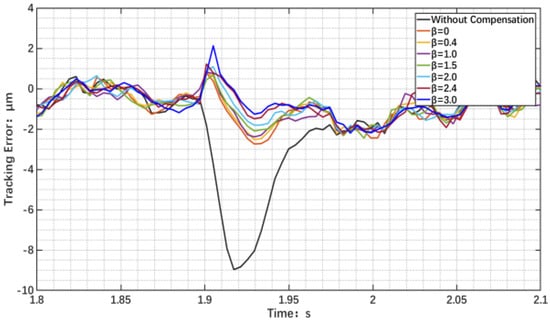
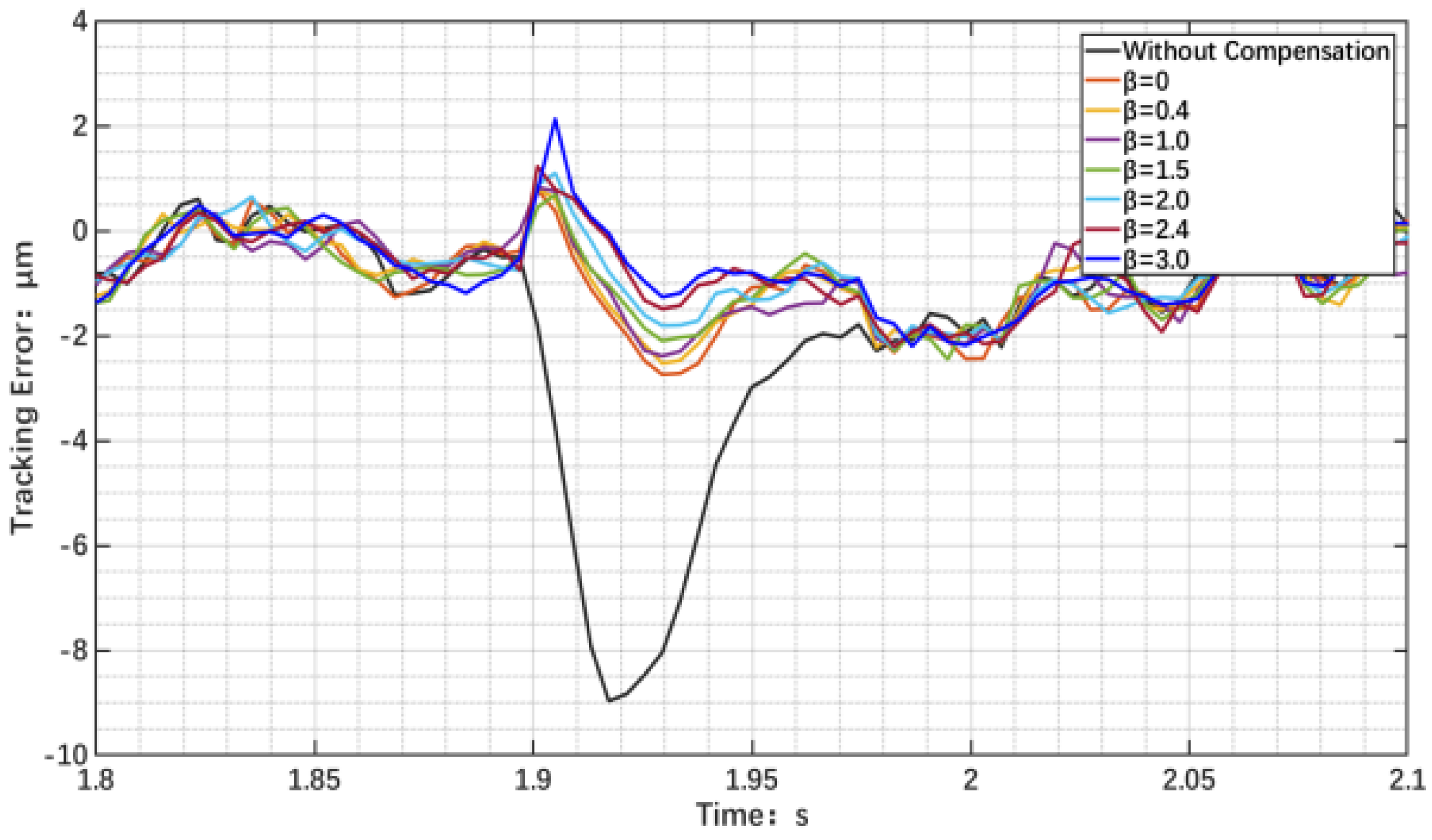
In the servo system, an X-axis cosine displacement command was applied to determine the value of the dynamic parameter β in the SDFM. The command signal corresponded to an average linear velocity of 3000 mm/min for the circular interpolation trajectory. In this experiment, the compensation value Δe was set to 4.5 μm and the compensation coefficient Φ was set to 0.6. The experimental results are shown in Figure 8.

Figure 8. The Effect of Dynamic Parameter β on Friction Compensation.

As the value of the dynamic parameter β increases, the single-axis tracking error of the feed system during reversal under high-speed conditions gradually decreases. However, the degree of overcompensation in the initial stage of reversal correspondingly increases. Taking into account both the compensation performance of the friction model at high speeds and the overcompensation observed in the initial reversal stage, the dynamic parameter was ultimately set to β = 2.4.

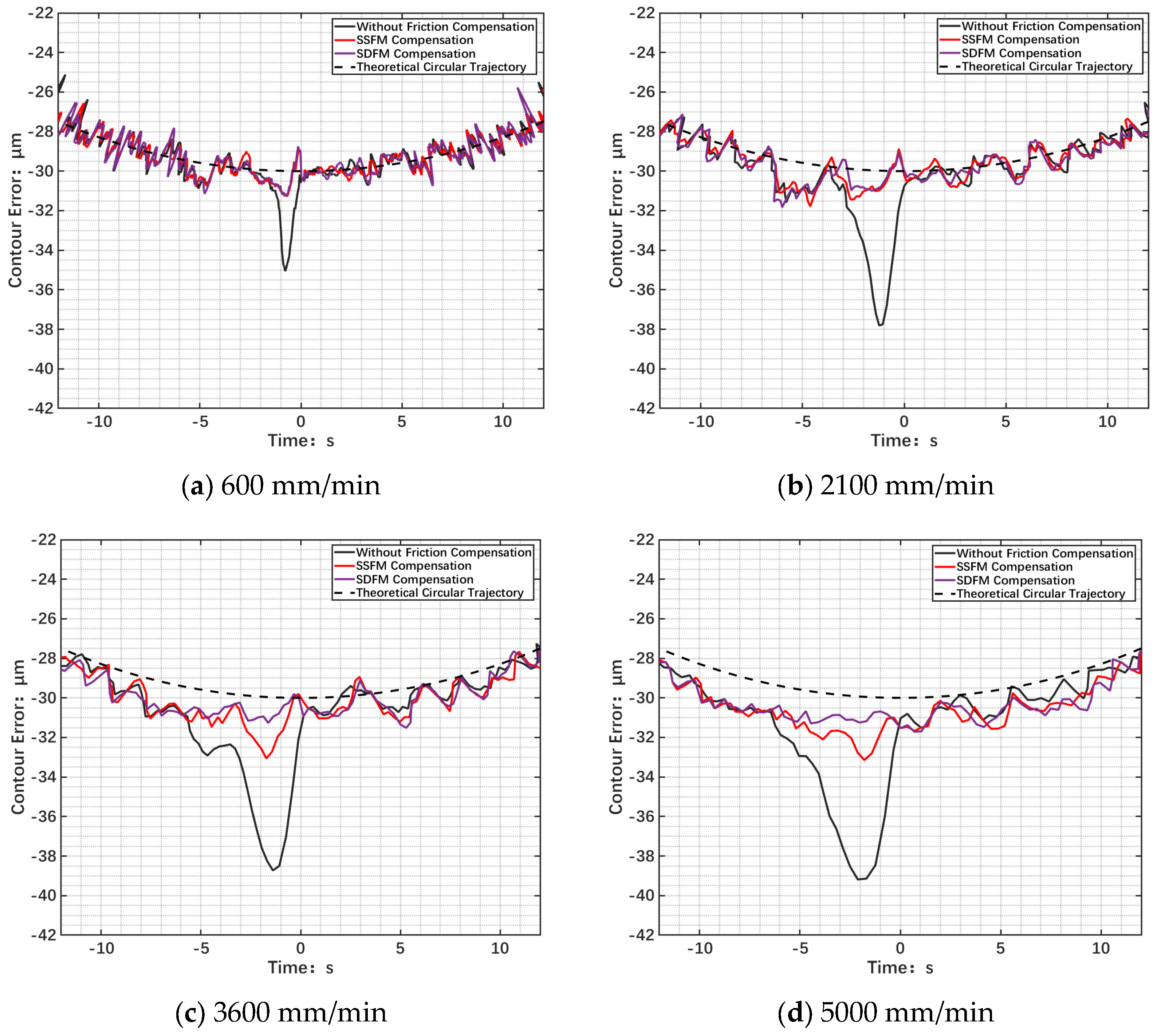
To verify whether the optimized compensation method can meet the requirements of precise compensation under high-speed operating conditions, a multi-axis circular interpolation machining experiment was conducted on the three-axis engraving–milling machine platform, applying the SDFM for friction compensation. The dynamic friction coefficient β was set to 2.4, the compensation value Δe was set to 4.5 μm, and the compensation coefficient Φ was set to 0.6. The velocity conditions were the same as those used in the previous experiment. By recording and analyzing the contour errors under each velocity condition, the control performance and compensation effectiveness of the system were evaluated. The experimental results are presented in Figure 6 and Table 1.

Table 1. Comparison of Contour Error Compensation Using the Simplified Friction Model.

Velocity (mm/min)	Without Friction Compensation (μm)	SSFM Compensation (μm)	SDFM Compensation (μm)
600	5.07	1.35	1.34
2100	7.75	1.61	1.22
3600	8.75	3.05	1.44
5000	9.24	3.21	1.49

Figure 9 shows the contour error compensation results based on the SDFM under different velocity conditions, and Table 1 presents a comparison of compensation performance using the simplified friction model. According to the experimental data in Table 1, under the velocity conditions of 3600 mm/min and 5000 mm/min, the maximum contour error of the feed axis was reduced from 3.05 μm and 3.21 μm with the SSFM compensation to 1.44 μm and 1.49 μm, respectively, after applying the improved SDFM. The compensation performance under high-speed conditions was significantly enhanced, and at low speeds, the improved method was still able to maintain satisfactory compensation effectiveness.

Figure 9. Contour Error Compensation Using the SDFM.

To further evaluate the repeatability of the proposed SDFM-based friction compensation method, three consecutive compensation experiments were carried out under four operating speed conditions. The maximum contour errors obtained from the repeated tests were used for statistical analysis, and the corresponding mean, variance, and standard deviation were calculated. The statistical results are presented in Table 2.

Table 2. Statistical results of three repeated compensation experiments under four speed conditions.

Velocity (mm/min)	Mean (μm)	Variance (μm2)	Standard Deviation (μm)
600	1.37	0.0082	0.0907
2100	1.35	0.0019	0.0436
3600	1.49	0.0007	0.0265
5000	1.51	0.0043	0.0656

As shown in Table 2, the standard deviations of the repeated experimental results remain at a relatively low level under all four operating speed conditions, indicating that the proposed SDFM has good repeatability. The maximum and minimum standard deviations are 0.0907 μm and 0.0265 μm, respectively, which suggests that the variation among consecutive repeated experiments is limited. Although the experimental results may still be influenced by factors such as encoder resolution, signal noise, servo lag, and unmodeled disturbances, the statistical results provide supporting evidence, from an engineering perspective, for the reliability of the compensation performance reported in this study.

Overall, based on the experimental data in the table, compared with the initially designed SSFM, the SDFM expands the velocity adaptation range of compensation. It achieves excellent compensation performance under low-speed operating conditions while providing superior effectiveness at medium and high speeds. With this optimization, the maximum friction force can better adapt to variations in different motion states, thereby enhancing the ability of the friction model to compensate for nonlinear friction across a wide range of operating velocities.

To further clarify the characteristics of the proposed method, a summary comparison with representative friction compensation models is provided. As shown in Table 3, classical friction models and compensation methods, including the Stribeck model, Karnopp model, LuGre model, adaptive friction compensation methods, neural-network-assisted friction compensation methods, and the proposed models, are compared from both mathematical and practical perspectives. For the methods reported in the literature, only the characteristics explicitly available in the corresponding references are summarized. Detailed quantitative results are reported for the proposed methods, while the numerical results of other methods are listed only when directly comparable data are available.

Table 3. Summary comparison of representative friction compensation methods and the proposed models.

Method	Model Type	Internal State	Main Parameters	Dynamic Friction Description	Parameter Identification	Real-Time Implementation	Typical Reported Advantage	Main Limitation
Stribeck	Static model	No	Moderate	Limited	Moderate	Good	Captures velocity-dependent friction decay	Cannot describe presliding dynamics well
Karnopp	Piecewise static model	No	Few	Limited	Relatively simple	Good	Simple structure and easy implementation	Piecewise switching may reduce smoothness near zero velocity
Classical LuGre	Dynamic model	Yes	Many	Strong	Complex	Moderate	Good physical interpretability and dynamic friction description	Parameter identification is difficult and computational burden is relatively high
Adaptive friction compensation	Adaptive/model-based	Usually yes or model-dependent	Many	Moderate to strong	Complex	Moderate	Improved robustness to parameter variation	Controller design and online tuning are more complicated
SSFM	Reduced-order dual-segment static model	No	2	Moderate in the reversal region	Simple	Excellent	Compact structure and effective reversal compensation at low-to-medium speeds	Compensation performance degrades at high speeds
SDFM	SSFM with acceleration-dependent dynamic correction	No	3	Improved in the high-speed reversal region	Simple	Excellent	Better adaptability under high-speed reversal conditions	Still simplified and limited in describing full internal friction dynamics

As shown in Table 3, the proposed SSFM and SDFM differ from representative existing methods in both modeling objective and implementation complexity. Classical models such as the Stribeck and Karnopp formulations are simple and computationally efficient, but their ability to characterize friction nonlinearity around velocity reversal is limited. The LuGre model and adaptive friction compensation methods provide richer dynamic descriptions or stronger nonlinear fitting capability, but they generally involve more parameters, internal states, or more complicated identification, training, and tuning procedures. By contrast, the proposed SSFM and SDFM are developed as reduced-order compensation-oriented models for the reversal region of CNC feed systems. In particular, the SDFM introduces an acceleration-dependent correction while preserving a compact structure, which improves compensation performance under high-speed conditions. Therefore, the proposed framework provides a practical balance among model simplicity, compensation effectiveness, and real-time implementability.

4. Conclusions

In response to the problem of significant contour errors caused by nonlinear friction during feed axis reversals in machine tools, a simplified static friction model was designed for friction feedforward compensation. Experimental results revealed that the compensation effectiveness of the simplified static friction model remained around 75% at low-to-medium speeds, but dropped to approximately 65% at high speeds.

To address the decline in compensation performance of the simplified static friction model at high speeds, the model was further developed into a simplified dynamic friction model and experimentally validated. The results demonstrated that, while maintaining compensation effectiveness at low-to-medium speeds, the simplified dynamic friction model improved the compensation performance at high speeds from about 65% to approximately 85%.

Although the proposed simplified models exhibit good compensation performance, the present study mainly focuses on model construction and experimental validation, while the parameter determination process still relies on empirical tuning. This limitation may affect the global optimality and repeatability of parameter selection. Therefore, future work will consider introducing systematic parameter identification and optimization strategies to further enhance model accuracy, robustness, and engineering applicability.

References

- Gao, B.; Shen, W.; Zheng, L.; Zhang, W.; Zhao, H. A review of key technologies for friction nonlinearity in an electro-hydraulic servo system. Machines 2022, 10, 568. [Google Scholar] [CrossRef] [Scilit]
- Liu, C.-C.; Tsai, M.-S.; Lin, M.-T.; Tang, P.-Y. Novel multi-square-pulse compensation algorithm for reducing quadrant protrusion by injecting signal with optimal waveform. Mech. Mach. Theory 2020, 150, 103875. [Google Scholar] [CrossRef] [Scilit]
- Xiao, Q.; Wan, M.; Qin, X. Pre-compensation of Friction for CNC Machine Tools through Constructing a Nonlinear Model Predictive Scheme. Chin. J. Mech. Eng. 2023, 36, 119. [Google Scholar] [CrossRef] [Scilit]
- Sheng, Y.; Wang, G.; Sang, L.; Li, D. A Novel Friction Compensation Method for Machine Tool Drive Systems in Insufficient Lubrication. Sensors 2024, 24, 4820. [Google Scholar] [CrossRef] [Scilit] [PubMed]
- Olejnik, P.; Ayankoso, S. Friction modelling and the use of a physics-informed neural network for estimating frictional torque characteristics. Meccanica 2023, 58, 1885–1908. [Google Scholar] [CrossRef] [Scilit]
- Li, B.; Xie, X.; Yu, B.; Liao, Y.; Fan, D. High-precision velocity control of direct-drive systems based on friction compensation. Mech. Sci. 2024, 15, 385–394. [Google Scholar] [CrossRef] [Scilit]
- Liu, M.; Zhu, Y.; Xu, H.; Liu, W.; Yang, H.; Gao, X. Pre-Compensation Strategy for Tracking Error and Contour Error by Using Friction and Cross-Coupled Control. Machines 2024, 12, 593. [Google Scholar] [CrossRef] [Scilit]
- Zhou, Q.; Liu, W.; Cang, Y.; Xu, K.; Gong, H.; Zhou, Y. Radial Basis Function Neural Network and Feedforward Active Disturbance Rejection Control of Permanent Magnet Synchronous Motor. Appl. Sci. 2024, 14, 7930. [Google Scholar] [CrossRef] [Scilit]
- Xi, T.; Fujita, T.; Kehne, S.; Ikeda, R.; Fey, M.; Brecher, C. An extended LuGre model for estimating nonlinear frictions in feed drive systems of machine tools. Procedia CIRP 2022, 107, 452–457. [Google Scholar] [CrossRef] [Scilit]
- Han, J.; Cheng, H.; Shan, X.; Liu, H.; Xiao, J.; Huang, T. A novel multi-pulse friction compensation strategy for hybrid robots. Mech. Mach. Theory 2024, 201, 105726. [Google Scholar] [CrossRef] [Scilit]
- Ma, L.; Lou, X.; Jia, J. Neural-network-based boundary control for a gantry crane system with unknown friction and output constraint. Neurocomputing 2023, 518, 271–281. [Google Scholar] [CrossRef] [Scilit]
- Yuan, S.; Yi, W.; Yang, G. Adaptive robust control of electromagnetic actuators with friction nonlinearity and uncertainty compensation. Math. Models Eng. 2024, 10, 75–86. [Google Scholar] [CrossRef] [Scilit]
- Rathee, R. Numerical modeling and simulation of friction models for mechanical systems: A brief review. Mater. Today Proc. 2023, in press. [Google Scholar] [CrossRef] [Scilit]
- Liu, Q.; Shen, S.; Ma, Y.; Li, B. A friction compensation approach of a 6 axis hybrid robot by considering joint inertia change. iScience 2025, 28, 112173. [Google Scholar] [CrossRef] [Scilit] [PubMed]
- Feng, H.; Yin, C.; Cao, D. Trajectory tracking of an electro-hydraulic servo system with a new friction model-based compensation. IEEE/ASME Trans. Mechatron. 2022, 28, 473–482. [Google Scholar] [CrossRef] [Scilit]
- Wan, M.; Dai, J.; Zhang, W.H.; Xiao, Q.-B.; Qin, X.-B. Adaptive feed-forward friction compensation through developing an asymmetrical dynamic friction model. Mech. Mach. Theory 2022, 170, 104691. [Google Scholar] [CrossRef] [Scilit]
- Wang, C.; Peng, J.; Pan, J. A novel friction compensation method based on Stribeck model with fuzzy filter for PMSM servo systems. IEEE Trans. Ind. Electron. 2023, 70, 12124–12133. [Google Scholar] [CrossRef] [Scilit]
- Dai, K.; Zhu, Z.; Shen, G.; Tang, Y.; Li, X.; Wang, W.; Wang, Q. Adaptive force tracking control of electrohydraulic systems with low load using the modified LuGre friction model. Control. Eng. Pract. 2022, 125, 105213. [Google Scholar] [CrossRef] [Scilit]
- Han, S.; Orzechowski, G.; Kim, J.-G.; Mikkola, A. Data-driven friction force prediction model for hydraulic actuators using deep neural networks. Mech. Mach. Theory 2024, 192, 105545. [Google Scholar] [CrossRef] [Scilit]
- Huang, D.; Yang, J.; Xu, G.; Chen, J. LuGre-Net: A hybrid neural network for friction modeling of feed systems in machine tools. Nonlinear Dyn. 2024, 112, 11927–11943. [Google Scholar] [CrossRef] [Scilit]
- Jiang, S.; Zhang, K.; Wang, H.; Zhong, D.; Su, J.; Liu, Z. Research on adaptive friction compensation of digital hydraulic cylinder based on LuGre friction model. Shock Vib. 2021, 2021, 8854424. [Google Scholar] [CrossRef] [Scilit]
Disclaimer/Publisher’s Note: The statements, opinions and data contained in all publications are solely those of the individual author(s) and contributor(s) and not of MDPI and/or the editor(s). MDPI and/or the editor(s) disclaim responsibility for any injury to people or property resulting from any ideas, methods, instructions or products referred to in the content. |
© 2026 by the authors. Licensee MDPI, Basel, Switzerland. This article is an open access article distributed under the terms and conditions of the Creative Commons Attribution (CC BY) license.