A Study of Tau-Robot Configuration for Friction Stir Welding

Abstract

This paper examines the use of high-rigidity Tau-robots in friction stir welding, where process loads are very high. The rigidity of Tau-robots increases at the expense of the workspace. Therefore, the right configuration of the Tau-robot is sought to reconcile rigidity and workspace requirements. This is studied by use of kinematics, followed by static and modal analysis. In particular, by extending an existing kinematic model employing free vectors, the robot workspace was derived in non-dimensional parametric form and was then maximized through evolutionary optimization. However, finite element static and modal analysis that were carried out subsequently may prove, as in a case demonstrated here, that the optimized configuration may not withstand high loads, typically axial forces of 15 kN and torques of 80 Nm, and it may also be susceptible to forced vibrations in the typical spindle rotation range up to 3000 rpm. As a rectification measure, it was shown how a modified configuration by placing robot kinematic chain bases further apart and shortening robot links achieves higher rigidity, axial displacement being reduced by one or two orders of magnitude to below 1 mm and increases critical modal frequency 3 to 5 times depending on the workspace position, of course sacrificing part of the workspace, i.e., reducing it 3-fold to enclose welding lines in a rectangle of dimensions 700 × 800 mm. In the quest for the appropriate robot configuration desired dimensions of parts to be welded and available standard components are briefly considered, too.

1. Introduction

Friction Stir Welding (FSW), since its invention by The Welding Institute (TWI) in 1991, has become a key technology for joining lightweight materials, particularly aluminum alloys, due to its ability to produce high-quality welds with minimal distortion and excellent mechanical properties since the material remains largely in a solid state throughout the welding process [1]. Traditionally, FSW has been performed using rigid machine tools such as dedicated FSW machines, modified milling machines, or CNC machining centres. These platforms provide the high stiffness and precision needed to sustain the large axial forces and precise tool positioning required during welding [2]. However, machine-based FSW systems are typically expensive, inflexible, and require significant floor space, which limits their appeal for low-volume or large, complex parts [3]. To overcome these limitations, recent research has explored the use of industrial robots for FSW. Robots offer significant advantages: high flexibility, the ability to access complex geometries, reconfigurability for different tasks, and the potential for cost-effective automation in low-to-medium production volumes [4].

At a first approximation, the following requirements for the robot can be defined:

• Strength and power: The robot should be able to compensate for the developed loads.
• Robustness and precision: The compliance of the robot should be minimal so that the tool does not deviate from the desired path and is not affected by vibrations.
• Dexterity: At least 5 degrees of freedom are required to allow adjustment of both the position of the tool and the welding angles.
• Measurement and control: The robot should have position, force and temperature measurement sensors to adjust welding parameters through a control loop.

Despite its potential, robotic FSW has to overcome several technical issues. The primary limitation is the relatively low stiffness of standard industrial robots compared to machine tools [5], leading to path deviations under high process loads, especially during plunge and initial welding phases [6]. This compliance can result in defects such as voids, tunnel defects, or inconsistent weld properties [7]. In addition, thermal effects during welding can exacerbate robot positioning errors due to thermal expansion and changes in the mechanical properties of the links [8].

Parallel kinematic robots, such as the Tau type, offer a promising alternative. Their closed kinematic chains provide higher dynamic stiffness and better load distribution, potentially overcoming the compliance issues faced by serial robots at the expense of comparatively severely limited workspace [9]. In addition, their design, while stiff, introduces complex singularities and workspace boundaries that complicate trajectory planning and real-time control to manage both position and force simultaneously under dynamic loading, especially under high process loads [10]. Addressing these issues is critical to making Tau-robots a viable alternative to traditional FSW machine tools.

While parallel robot architectures have been proposed for FSW and isolated studies involving Tau or Gantry-Tau mechanisms exist, the gap identified concerns the investigation of an appropriate Tau-robot configuration that fulfils FSW requirements, balancing structural performance and workspace size in connection to intended welding seam shape and size. In this direction, the following three interrelated aspects are investigated in this work: (i) a parametric (dimensionless) geometric configuration of the Tau-robot open to optimization rather than predefined Tau-robot configurations, (ii) explicit stiffness–workspace trade-off for FSW conditions showing how geometry modification can restore stiffness at the expense of workspace rather than seeking workspace maximization or stiffness improvement separately, (iii) static and dynamic behaviour under representative FSW loads based on finite element static and modal analysis.

Following this introduction, an in-depth literature review is provided in Section 2. A succinct analysis of FSW is presented in Section 3. In Section 4, kinematic analysis and workspace determination of a parametrically defined Tau-robot are provided, leading to an optimal configuration. For this configuration, static and dynamic analysis under loading is presented in Section 5, resulting in a modified configuration. Its suitability for FSW is discussed in Section 6, including some implementation considerations. Conclusions and outlook are given in Section 7.

2. Literature Review

FSW process windows, tool design, and metallurgy are intertwined with robotics issues such as positioning accuracy, structural stiffness, and real-time control [4,8].

Early robot design for FSW focused on serial links; more recent work aims at optimization of structural members [11] and explores parallel robot topologies to push up stiffness without sacrificing workspace [12]. Redundant actuation and careful dimensional synthesis can make process parameter errors less important and redistribute internal forces [13]. Model-based stiffness prediction enables dimensioning of links and joints such that the end-effector deflection stays within tolerance across the envelope [14].

A comprehensive stiffness modelling framework for a 5-DoF hybrid manipulator designed for friction stir welding, incorporating both serial and parallel subsystem compliances, is presented in [15]. The model is analytically and experimentally evaluated to assess stiffness distribution and its impact on machining accuracy. A model-based approach for predicting the stability of robotic machining processes by coupling robot structural dynamics with manufacturing process force models enables identification of stable operating regions [16]. The performance of a Gantry-Tau parallel mechanism is evaluated in [17] through kinematic and experimental analysis.

Robotic FSW is dominated by load-induced deflection and thermal drift over trajectories [18]. Parameter studies reveal how feed rate, rotational speed, and tool geometry map to axial force transients that controllers must gracefully absorb to avoid chatter or wormhole defects [19]. Considering measured force in position loops enhances seam tracking and plunge robustness in the presence of fixture or geometry uncertainty [20,21]. By anticipating force-dependent deviations and pre-deforming the path, weld seam geometry and plunge consistency improve, especially on long curvilinear seams [22].

Digital-twins now embed finite-element thermal–mechanical models with robot dynamics, allowing verification of contact conditions, plunge depth, and force margins before hardware trials [23]. For complex space-curve welds (e.g., on monocoque structures), Tau-robot installation optimization using dynamic dual particle swarm methods determines the workpiece placement that maximizes stiffness margins and avoids kinematic singularities along the seam [24]. Kinematic sensitivity analysis and dimensional synthesis further guide the early-stage design of parallel robots with redundant degrees of freedom so that isotropy, transmission factors, and singularity loci are acceptable within the anticipated weld envelope [12].

In summary, robotic FSW has been improving through: (a) increased structural stiffness and improved load distribution achieved by parallel or hybrid kinematic architectures, (b) reduction in end-effector deflection through model-based stiffness optimization, (c) improved trajectory accuracy and seam quality through force-based control and feed-forward compensation methods, (d) enhanced process stability through dynamic modelling and digital-twin approaches. However, a practical trade-off is that workspace enlargement often leads to reduced structural stiffness and lower natural frequencies, which may compromise suitability for FSW. In addition, control-based compensation approaches may be effective in improving path accuracy, but do not eliminate the underlying mechanical compliance and therefore cannot fully replace structural optimization.

Robotic FSW applications continue to expand. Battery pack assembly in lightweight electric vehicles increasingly uses robotic FSW for extrusion-cast aluminum, where narrow flanges, high thermal mass, and dissimilar interfaces demand both stiffness and dexterous reach [25]. FSW using Temperature-Controlled Robotics and dissimilar materials joining has been reported for demanding applications, such as for high-pressure die-cast cylinder blocks [26]. Repair and retrofit use cases, e.g., of train sets, large aerostructures, etc., benefit from mobile or gantry-mounted Tau-robots with compliant fixtures maintaining weld quality even on thin skins and curved geometries [13,27]. Case studies confirm the existing practicality gap, namely, maintaining force and pose fidelity over large workspaces, on complex seams, under temperature-dependent material properties.

3. Load and Accuracy Requirements in Robotic FSW

The FSW tool consists of a specially shaped pin, usually with some type of helix on its perimeter and a shoulder which is of larger diameter and particularly robust. As the tool rotates, the pin of the tool penetrates the interface of the two materials to be welded. Due to the frictional forces, the temperature locally increases, and the materials enter the plastic domain, yet without melting. Due to the special geometry of the pin, the material is stirred and is transferred from the front (advancing side) to the back (retreating side) of the tool, where it cools due to the significant temperature difference in these two regions. There, in the presence of the pressure exerted by the shoulder of the tool, it solidifies completely [3]. The process is carried out by simultaneously advancing the tool along the interface. With additional material removal and/or grinding, the welding trace can literally disappear.

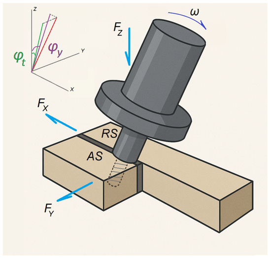
The so-called ‘rotating plug’ model is most commonly used for estimating the welding torque and power in FSW: M = 2πR³ (1 + 3 r² t/R³) Y/3 and P = Mω, where M/Ρ: the torque/power, Y: the yield strength of the material, r: the radius of the tool pin, R: the radius of the tool shoulder, t: the depth of the pin, and ω: the rotational speed of the tool [28]. Two additional parameters are the tilt angle (φ_t) and yaw angle (φ_y), see Figure 1.

Figure 1. FSW process setup (φ_t: tilt angle, φ_y: yaw angle, AS: advancing side, RS: retreating side).

Figure 1 also shows the developed forces on the workpiece in the steady state. The axial component FZ is responsible for the developed friction between the tool and the workpiece, contributing to the heat generation. In addition, it exerts pressure on the newly welded area, thereby improving weld quality. The frontal component FX results from the resistance of the cold material along the seam path. The lateral component FY is due to the asymmetry of the process, as the material on the advancing side is hotter and therefore softer compared to that on the retreating side [18].

The temperature in the yield zone varies little over a wide range of operating conditions. Therefore, the spindle power remains approximately constant over a wide range of speeds. Hence, the torque may be reduced if the process is carried out at high speeds [29], provided that the increase in frictional shear rate does not take over the thermal softening. Note that the axial force during the initial penetration of the tool into the workpiece also decreases with speed, but it can be up to three times higher than that observed during the welding seam generation by the tool following the welding path [6].

Typically, to cover a wide range of materials and configurations to be welded in practice, the spindle power should exceed 4 kW, and the working angle should be possible to vary between 0 and 5°. The developed loads reach up to 30 kN and 20 kN for the axial and lateral force, respectively [4,8], which are extremely high. However, for the case of aluminum alloys and polymers, load requirements are significantly lower, typically by a factor of 5–10 [30]. In [3], for instance, an extensive table is provided presenting welding parameters and tool dimensions for various cases of materials. As far as accuracy is concerned, the maximum deviations from the nominal size for weldments to be acceptable are position: ±1 mm, tilt angle: ±1°, yaw angle: ±2° [31,32].

4. Tau-Robot Parametric Kinematic and Workspace Analysis

The Tau-robot configuration can be implemented using either linear or rotary actuators. In the second case, the tool centre point (TCP) has only 3 degrees of freedom, i.e., its orientation is predetermined, and therefore, the type of welds that can be achieved is limited. In addition, the linear action is easier to construct; it corresponds to distributed loads on the actuator bases, enhancing robustness, and the corresponding kinematics solutions are known [33].

4.1. Forward Kinematics

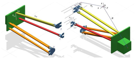
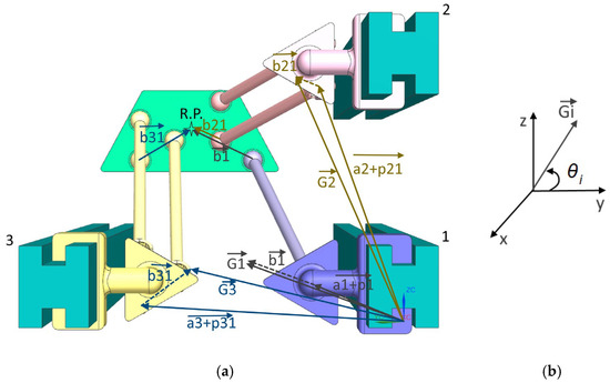
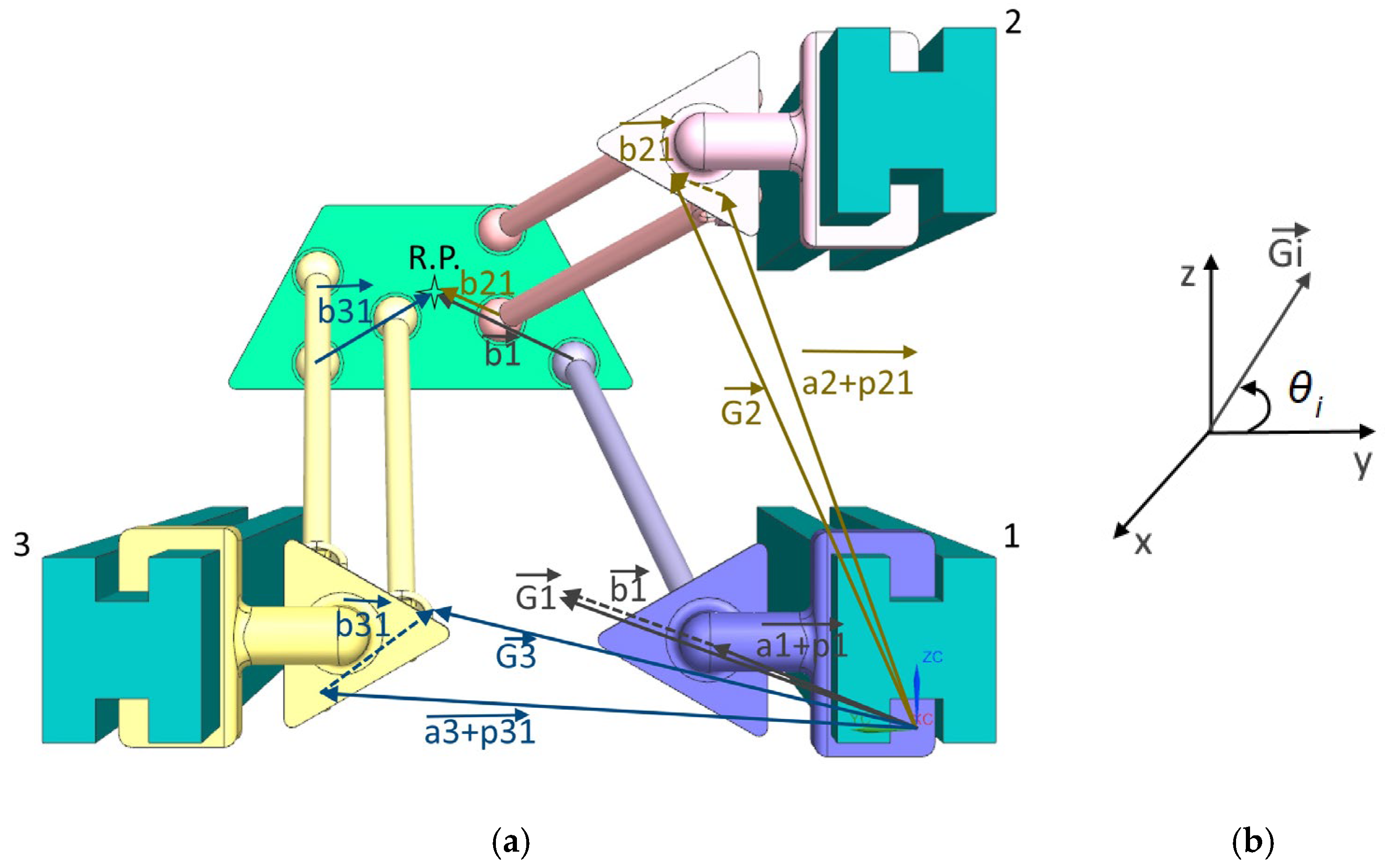
In Figure 2, the configuration of a linearly actuated Tau-robot is presented. Its kinematics analysis is summarized next, following the detailed treatise presented in [33]. The robot consists of three individual kinematic chains: the first having one arm (rod), the second having two arms parallel to each other, and the third having three arms, also parallel to each other. Each arm is connected via a 2 DoF Universal Joint (UJ) to the base, and via a 3 DoF Spherical Joint (SJ) to the final frame accommodating the TCP. The base of each chain is connected via a Prismatic Joint (PJ) to a linear guide. The actuation is performed on each of the three PJs along the linear guides.

Figure 2. Configuration of linearly actuated Tau-robot and its vectorial analysis (UJ: universal joint, PJ: prismatic joint).

The three DoFs, which constitute the control variables of the system, are denoted as $Q_i,i=\mathrm{1,2},3$. To simplify the kinematic equations, the global coordinate system is placed so that the global X-axis is parallel to the three linear guides, i.e., the three control variables take only positive values. The TCP is placed on the final frame, where all three individual kinematic chains end up and constitutes the Reference Point. The latter is defined in the global coordinate system by the position vector $\overrightarrow{R}$:

$$\overrightarrow{R}={\overrightarrow{a}}_i+{\overrightarrow{Q}}_i+{\overrightarrow{p}}_{ij}+{\overrightarrow{L}}_i+{\overrightarrow{b}}_{ij},i=\mathrm{1,2},3 j=1,...,i$$

(1a)

where (see Figure 2)

${\overrightarrow{a}}_i$: The position vector of the linear guide i;

${\overrightarrow{Q}}_i$: The linear DoF of guide i;

${\overrightarrow{p}}_{ij}$: The vector starting at the linear joint i and ending at spherical joint j of link i;

${\overrightarrow{L}}_i$: The length vector of link i;

${\overrightarrow{b}}_{ij}$: The vector from the spherical joint j, where link i ends, to the TCP.

Due to the Tau-configuration for each link i, the sums ${\overrightarrow{p}}_{ij}+{\overrightarrow{b}}_{ij},\forall j$ are equivalent to each other. Thus, all (known) constant terms add up to the vector ${\overrightarrow{G}}_i={\overrightarrow{a}}_i+{\overrightarrow{p}}_{ij}+{\overrightarrow{b}}_{ij}$ hence Equation (1a) becomes:

$$\overrightarrow{R}={\overrightarrow{G}}_i+\left\{\begin{array}{ccc}{L}_{ix}& L_{iy}& L_{iz}\end{array}\right\}+\left\{\begin{array}{ccc}{Q}_i& 0& 0\end{array}\right\}$$

(1b)

4.2. Dimensionless Equations

The robot workspace is mapped by assigning numerical values to the (constant) geometric entities involved. This is also necessary because it is impossible to express analytically the geometric constraints that ensure the closed nature of kinematic chains. Given the lack of experience in designing and using Tau-robots, it was decided to optimize a dimensionless configuration of the robot. The optimization criterion is the increase in the robot workspace.

The maximum travel of any DoF is defined as Q, thus $Q_i\in [0,Q]$. Then, new dimensionless variables are defined as follows:

$$q_i={\displaystyle \frac{Q_i}{Q}},q_i\in \left[\mathrm{0,1}\right], r_j={\displaystyle \frac{R_j}{Q}},g_{ij}={\displaystyle \frac{G_{ij}}{Q}},l_{ij}={\displaystyle \frac{L_{ij}}{Q}}j=x,y,z i=\mathrm{1,2},3$$

(2)

Thus, the new system of equations defining the robot’s kinematics is expressed as follows (compare with Equations (1a) and (1b):

$$\left\{\begin{array}{c}{r}_x=g_{ix}+l_{ix}+q_i\\ r_y=g_{iy}+l_{iy}\\ r_z=g_{iz}+l_{iz}\end{array}\right\},i=\mathrm{1,2},3$$

(3)

and

$$l_{ix}^2+l_{iy}^2+l_{iz}^2=c_i,i=\mathrm{1,2},3$$

(4)

where

$$c_{is}=\sqrt{c_i}={\displaystyle \frac{\left|L_i\right|}{Q}}$$

(5)

The unknowns are r_x, r_y, r_z, l_ix, l_iy, l_iz, i = 1,2,3.

Similarly, the corresponding dimensionless geometric parameters are:

$$g_{ix}^2+g_{iy}^2+g_{iz}^2 =k_i,i=\mathrm{1,2},3$$

(6)

where

$$k_{is}=\sqrt{k_i}={\displaystyle \frac{\left|G_i\right|}{Q}}$$

(7)

An additional dimensionless factor that quantifies the proportionality of link size with respect to other structural quantities is defined as:

$$m_i={\displaystyle \frac{c_{is}}{k_{is}}}$$

(8)

Note that (a) each vector ${\overrightarrow{L}}_i$ has a constant magnitude but its orientation is variable and generally unknown, and (b) each vector ${\overrightarrow{G}}_i$ has a constant magnitude and constant and known orientation. Therefore, by introducing the unit vector ${\widehat{G}}_i$, the following expression holds:

$${\overrightarrow{G_i}={\widehat{G}}_i\Vert \overrightarrow{G_i}\Vert \Rightarrow g}_{ix}={\displaystyle \frac{{\widehat{G}}_{ix}\Vert \overrightarrow{G_i}\Vert }{Q}}={\widehat{G}}_{ix}{k}_{is},i=\mathrm{1,2},3$$

(9)

In Figure 3a, the vectors involved in defining the constant geometry of the configuration are depicted. As a default, ${\overrightarrow{G}}_1$ is positioned between ${\overrightarrow{G}}_2,{\overrightarrow{G}}_3$. Furthermore, using a suitable global coordinate system definition, ${\overrightarrow{G}}_{ix}$ can be neglected, yielding ${\widehat{G}}_i=\left\{0,\cos \left( {\theta }_i\right),\cos \left( {\theta }_i-{90}^0\right)\right\}$; see Figure 3b.

Figure 3. (a) Constant vectors of the robot’s geometry (view from behind). (b) Vector ${\overrightarrow{G}}_i$.

4.3. Optimization of Dimensionless Variables

The vector to be optimized is:

$$\overrightarrow{x}=\left\{{\theta }_1,{\theta }_2,{\theta }_3,m_1,m_2,m_3,c_{1s},c_{2s},c_{3s}\right\}$$

(10)

The applicable constraints are: an upper bound: $\left\{\mathrm{85,85,85,100,100,100,2},\mathrm{2,2}\right\}$, a lower bound: $\left\{-85,-85,-\mathrm{85,0.1,0.1,0.1,0.1,0.1,0.1}\right\}$ and ${\theta }_3\le {\theta }_1\le {\theta }_2$.

The upper and lower bounds were set as follows. Preliminary exploratory runs and CAD-based geometric trials showed that very small parameter values lead to fragmented or extremely limited workspaces, whereas excessively large values generate elongated configurations with poor geometric conditioning and reduced structural realism. In addition, the adopted intervals were chosen so that the nonlinear kinematic system remains numerically stable and yields a sufficient percentage of real (physically meaningful) solutions during optimization. Although the model is dimensionless, the selected bounds also reflect typical proportional ranges encountered in Tau-type mechanisms, avoiding configurations that would be impractical. Therefore, the optimization bounds represent a compromise between workspace enlargement, computational efficiency and realistic geometric proportions.

Trying out a sufficiently large number of vector values in a ‘brute force’ mode would be computationally very intensive since at each and every point, a 12 × 12 system of equations needs to be solved, corresponding to a total computation time of the order of 24 h for a dense mesh of points. Therefore, a relatively sparse mesh of points is adopted, and solutions for $Q_i$ are sought not in the interval $\left[\mathrm{0,1}\right]$ but in its subset $\left[\mathrm{0.3,0.7}\right]$. This selection resulted from repeated trials using a selection of different robot dimensions to define robot models in a CAD environment. The choice was validated by considering the shape of the workspace at the end of this section.

Furthermore, instead of maximizing the workspace volume, it was chosen to minimize the percentage of unacceptable solutions in a reference volume discretized as a reasonably sparse mesh.

Optimization was performed through a classic genetic algorithm that was set up in Matlab^TM R2020b optimization toolbox, using mostly the system default parameter values except for the following:

(a)

Population set to 50 instead of the default 200 chromosomes to reduce execution time;

(b)

Elitism set to 1 chromosome;

(c)

Termination condition: Either 30 generations or minimization of the objective function within 0.001, whichever occurs first.

Upper and lower bounds for variables were defined with an accuracy of 0.01.

The objective function simply counts the number of inaccessible points. To do so, the end-effector is positioned at each and every point of the mesh. Then, the inverse kinematics solutions are derived, and their acceptability is evaluated with the aim of labelling them accessible or inaccessible. Note that the 12 × 12 system of equations that is solved at each point always yields two mathematical solutions for each end-effector position coinciding with the point under consideration. This occurs because the closure equations of the Tau-robot allow two geometrically feasible configurations (poses) that satisfy the same end-effector coordinates. However, these are just mathematically admissible solutions and not necessarily physically meaningful. The counter of accessible points is therefore increased by one if both conditions hold. A complex number solution is rejected by definition. Furthermore, the workspace should not contain points that correspond to any collision between links, but this is expensive and difficult to express. Thus, duplicate solutions are avoided by just setting $L_{ix}>0$, i.e., links are turned towards the positive global $\widehat{x}$ and not the other way around.

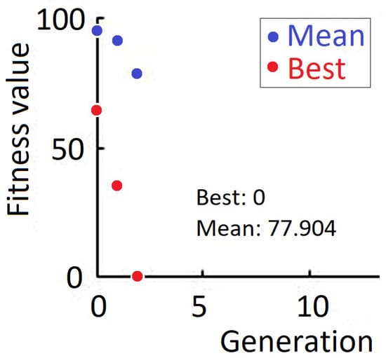
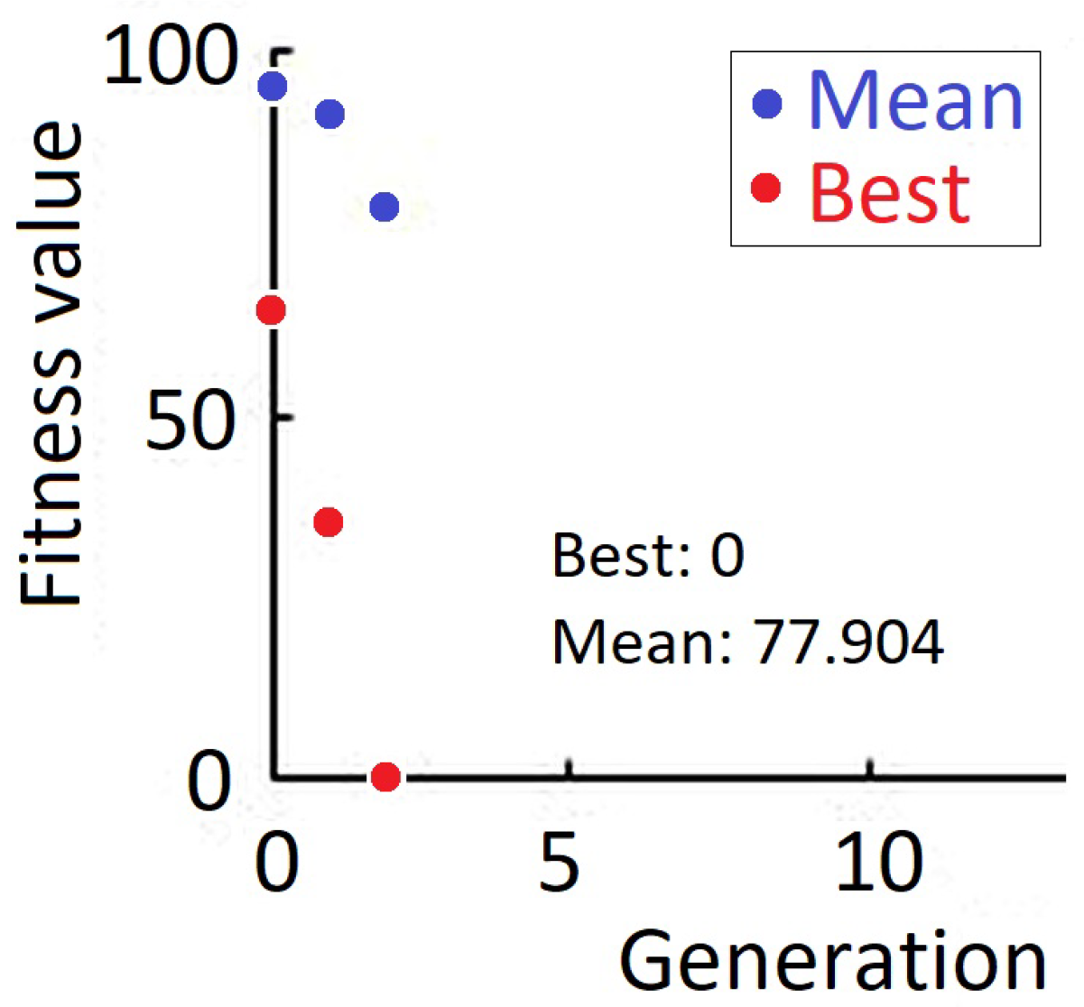
The convergence history of the genetic algorithm is shown in Figure 4. The fitness of the average chromosome does not fall so fast, but the best chromosome does indeed. The difference between the mean (77.9) and best (0) fitness values is large enough to prove the existence of diversity in the population. Since the absolutely best solution was found, i.e., the one corresponding to all points examined being accessible with that particular robot configuration, it was thought to be superfluous to allow the genetic algorithm to run for more generations. This is due to the computational cost of the inverse kinematics solution, being applied exhaustively for all the points of the potential workspace.

Figure 4. Evolution history of the genetic algorithm solution.

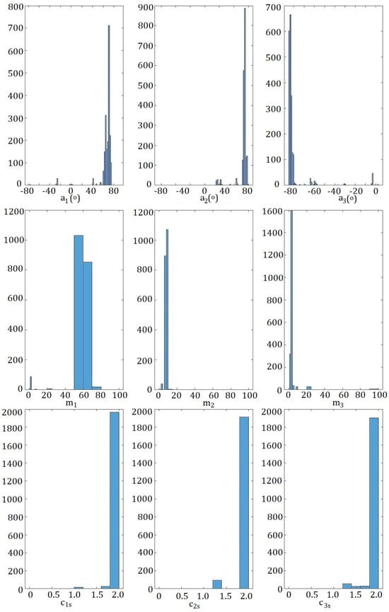
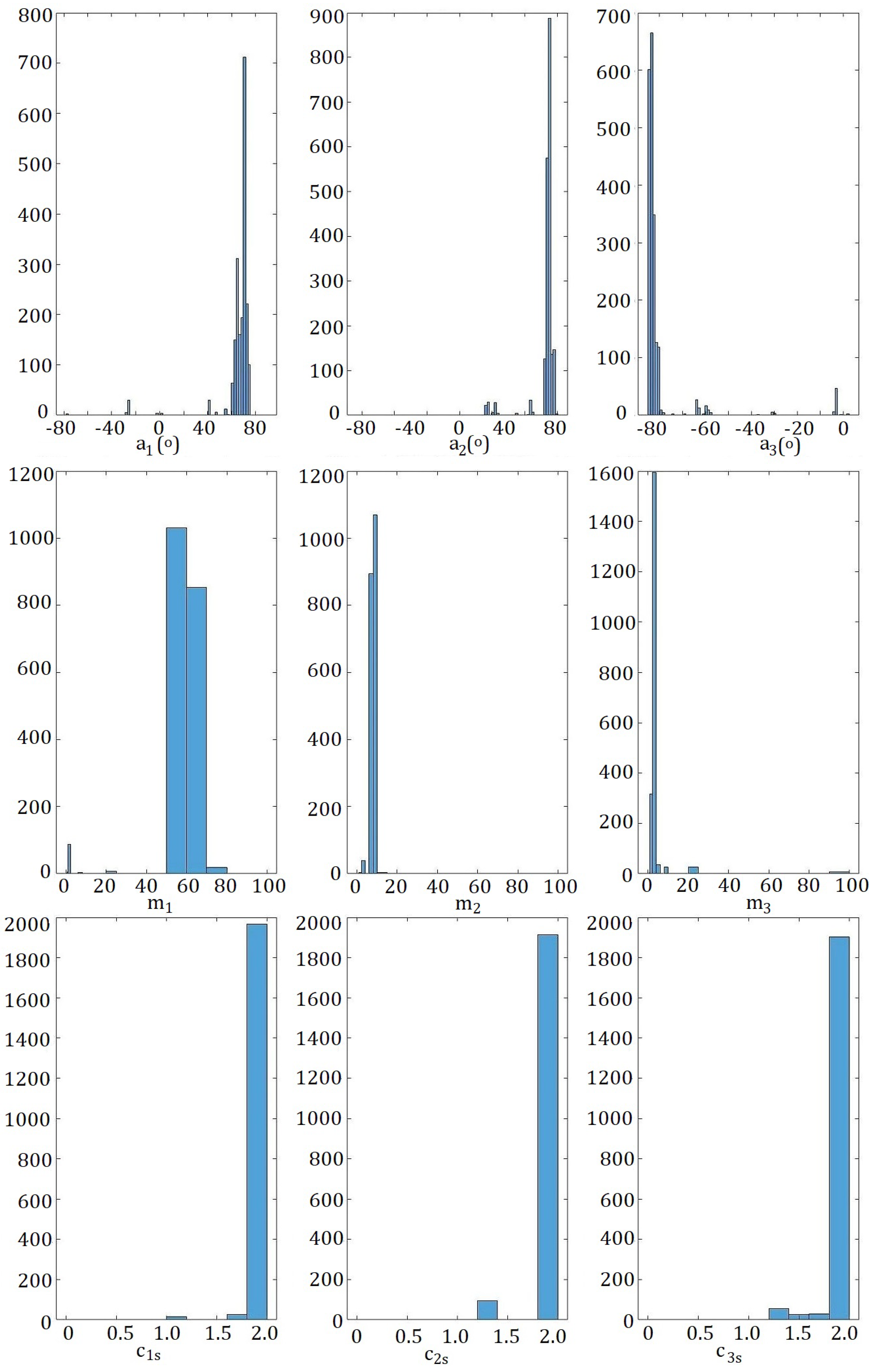
The results are shown in histogram form in Figure 5, for each parameter. Overall, a low non-accessibility percentage is achieved $(P<3\mathrm{\%})$. The best solution turns out to be {$70^0, 75^0,-83^0,60, 8, 3, 2, 2, 2\}$.

Figure 5. Optimization of angles ${\overrightarrow{\theta }}_i$, coefficients m_i and coefficients c_is.

Furthermore, m₁ = 60 >> m₂ = 3 > m₃ = 2, i.e., link 1 is much longer than links 2 and 3, which is in agreement with the position of the coordinate system origin on the guide of link 1, i.e., with a low contribution of ${\overrightarrow{a}}_1$ and ${\overrightarrow{p}}_{11}$.

As far as coefficients c_is are concerned, they tend to their maximum allowable values, thereby pointing to the need to use as long as possible links.

4.4. Workspace Computation

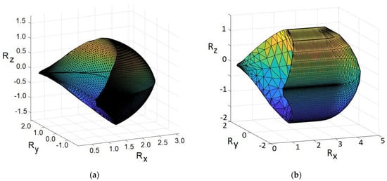
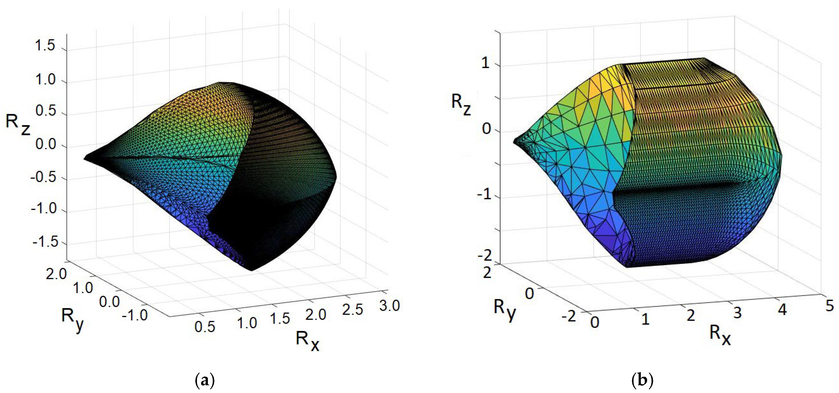
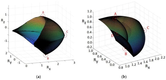
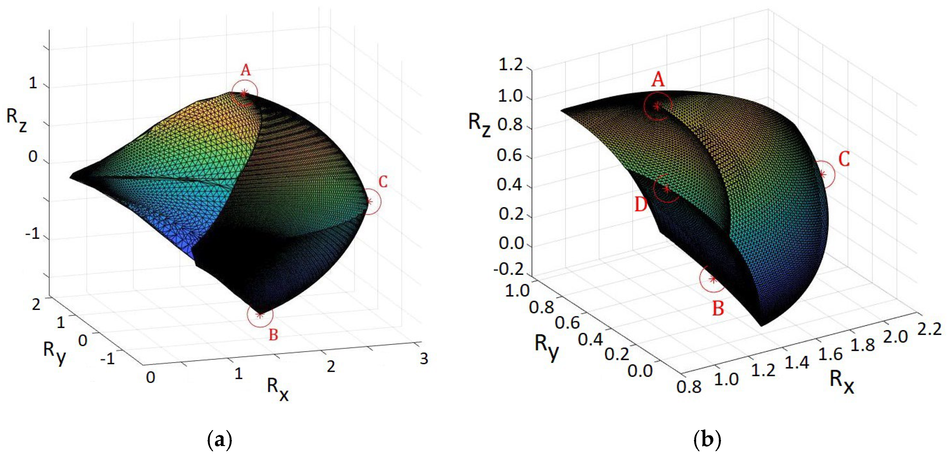
Based on the optimized Tau-robot configuration, as determined in the previous section, it is now possible to compute the coordinates (r_x, r_y, r_z) of the robot end-effector by using an appropriately small step equal to 0.1 for each DoF $Q_i\in \left[\mathrm{0,1}\right]$, thereby yielding the dimensionless workspace; see Figure 6a.

Figure 6. Dimensionless workspace (a) $Q_i\in \left[\mathrm{0,1}\right]$ and (b) $Q_i\in \left[\mathrm{0,3}\right]$.

The domain is arc-shaped, and its volume is $v_{wspc}=5.0625$. If the length of the links is increased by using $c_{is}=5$ or even $c_{is}=10,i=\mathrm{1,2},3$, keeping all the rest parameters invariable, the workspace volume is computed as $v_{wspc}=14.5970$ or $26.3137$ correspondingly, i.e., significantly higher. In fact, it is not necessary for Q to correspond to the maximum length of the links. For example, in Figure 6b, the dimensionless workspace corresponding to $Q_i\in \left[\mathrm{0,3}\right]$ is $v_{wspc}=22.3$, i.e., 5.4 times larger than the initial one.

The shape of the robot workspace seems suitable for FSW of planar or near-planar surfaces extending along Ζ or along Ζ axes. However, the suitability of the Tau-robot is still to be confirmed from both strength and dynamics points of view.

5. Tau-Robot Static and Modal Analysis

An important feature of the robot is its robustness, which for complex models can only be determined by numerical/finite element analysis (FEA) methods [23,33]. For this reason, it is chosen to perform static analysis and modal analysis of a dimensioned instance of the robot in some indicative poses while maintaining the optimized ratio coefficients of the dimensionless case.

The robot instance’s loads correspond to welding of aluminum alloys, i.e., F_z = 15 kN, F_x = 2 kN, as well as M_z = 80 Nm for the case of maximum power of 4 kW, and maximum speed of 3000 rpm. The first eigenfrequency must be greater than the critical operating frequency, i.e., f_c = 50 Hz (3000 rpm). It is noted that the modal analysis is simplified as internal damping of the components is not considered.

Thus, applying Q = 1 m to Equations 1–9, the following values are obtained: c_is = 2, L₁ = L₂ = L₃ = 2 m, k_is = {0.03 0.25 0.67}, {G₁ G₂ G₃} = {0.03 0.25 0.67}.

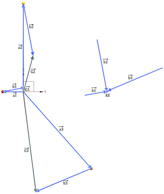
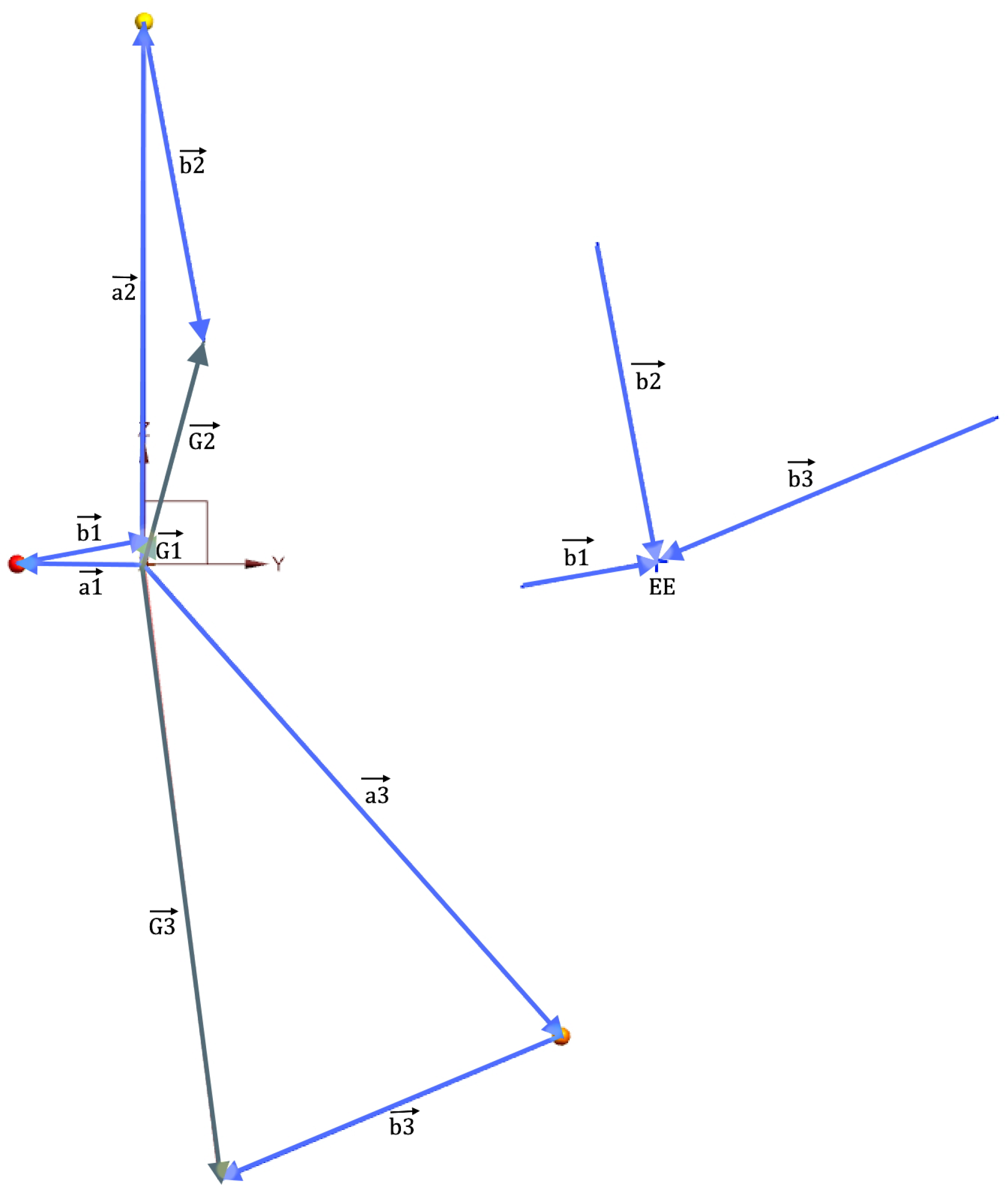
From Equations (6) and (9), the geometric constants ${\overrightarrow{G}}_i$ are obtained, and the individual components that make it up are free to choose. Thus, seeking the greatest possible separation of linear vectors, the vectors of Figure 7 are selected. The End-Effector (EE) is the point of reference and the intersections ${\overrightarrow{b}}_i$ ending on it are transferred to the end of the corresponding ${\overrightarrow{a}}_i$ to compute the respective ${\overrightarrow{G}}_i$.

Figure 7. Selection of geometric fixed vectors (EE: end-effector).

A space of 400 × 400 mm is provided at the EE to accommodate a 4 kW/3000 rpm motor, and a typical FSW tool of diameter of Ø8 mm is placed at its end. The links and bases are simplified for kinematic modelling; see Figure 2.

The 3D models of the robot were created in the Siemens NX^TM 3D CAD environment, whilst FEA was conducted in the ANSYS^TM R19 environment. Note that, due to the nature of the welding, there are no large inertial loads, and the main stress is due to the large imposed loads. Therefore, the static study in critical poses of the device offers essential information on the suitability of the robot.

The following quantities are determined from the study:

• Displacement of the EE under the applied loads. This is the open-loop behaviour, which should be in the order of a few mm before applying any control.
• Maximum loads on the bases aiming to determine the requirements on the supports and actuators.
• Maximum stresses on the links aim to check the adequacy of the cross-section.

5.1. Static Analysis

The link rods are assigned a diameter of 75 mm and are made of tool steel DIN 1.2738 (σ_Υ = 980 MPa). They are modelled as deformable bodies, whereas the bases, U- and S-Joints, end-plate and workpiece are modelled as rigid bodies. Rigid joints correspond to the respective DoFs, whereas the bases and the workpiece are fixed. The loads on the tool are modelled as joint loads. The loads are F_z (local axial) = 15 kN, F_x (local side) = 2 kN, M_z (local axial) = 80 Nm. Two alternatives for the welding line direction are considered, namely: along the global Z-axis (WLZ) and along the global X-axis (WLX).

In case WLZ, the main load in the axial direction is in the global X direction; therefore, the stiffness is higher than in case WLX. However, in case WLX, the welding path can be of any desired length and, in addition, no significant changes in the robot pose are expected (hence in system dynamics, too).

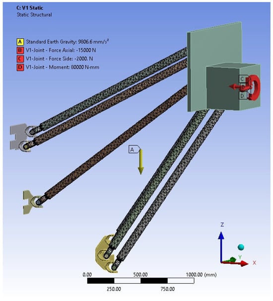
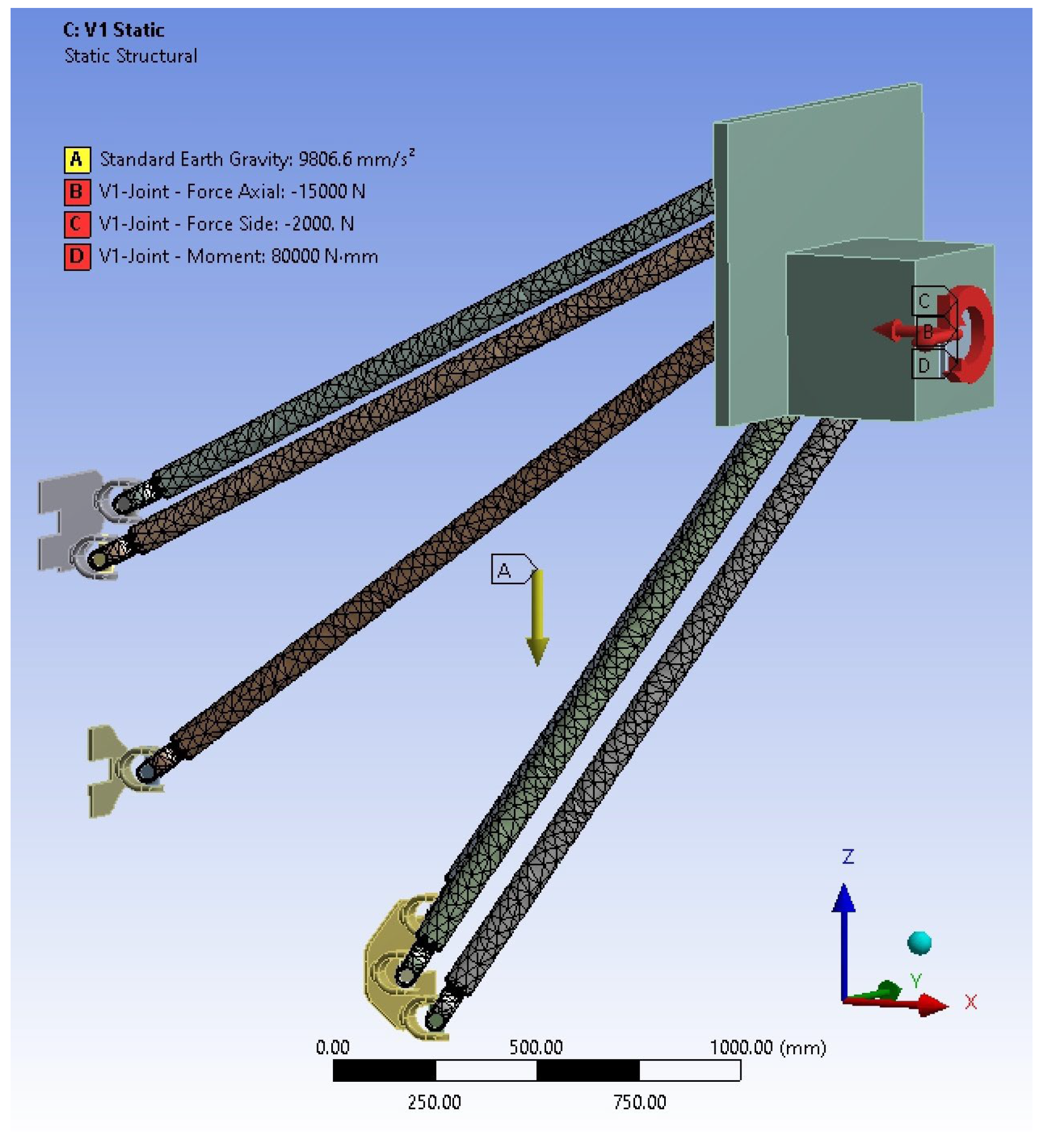
Adaptive Meshing of tetrahedra and trihedra of general size ‘fine’ is adopted in Ansys^TM. Two element sizes were tried, namely 40 mm and 15 mm, resulting in an average number of elements per link equal to 10,253 and 30,047, respectively. The results corresponding to the same loading scenario (see Figure 8) are shown in Table 1. The largest difference between large and small element sizes emerged in the max von Mises stress cases. This reflects the need to use finer elements when geometry becomes more intricate at the end of the links, interfacing with connectors; the adoption of large elements there is likely to lead to stress singularities in view of idealized joint or boundary condition modelling. However, note that the already very low level of stress becomes even lower when smaller elements are employed, which is expected to approach reality more closely.

Figure 8. Model case WLZ.

Table 1. Mesh size influence (legend: Max_Stress_N-M: Max von Mises stress at link N, rod M).

Property	Element Size		Property	Element Size
	40 mm	15 mm		40 mm	15 mm
Max_Stress_1-1 (MPa)	8.8297	4.6525	Ftotal Base 1 (kN)	9.668	9.675
Max_Stress_2-1 (MPa)	10.537	5.7171	Ftotal Base 2 (kN)	25.827	25.831
Max_Stress_2-2 (MPa)	13.411	7.2219	Ftotal Base 3 (kN)	1.820	1.818
Max_Stress_3-1 (MPa)	0.6619	0.8245	Mtotal Base 1 (kNm)	6.4553	6.4601
Max_Stress_3-2 (MPa)	6.5340	3.5953	Mtotal Base 2 (kNm)	2.2888	2.3292
Max_Stress_3-3 (MPa)	5.0508	2.8647	Mtotal Base 3 (kNm)	1.7672	1.7638
Side Displacement (mm)	1.4024	1.4169	Ftotal Clamp (kN)	17.361	17.369
Axial Displacement (mm)	−0.4191	−0.4238	Mtotal Clamp (kNm)	11.455	11.462

Figure 9a depicts the workspace points studied in both WLZ and WLX cases of the original configuration. Note that of the six characteristics points studied, only points A, B, and C are visible since the rest are occluded. Table 2 presents the coordinates of the six characteristic points studied.

Figure 9. Robot end-effector points studied: (a) original configuration, (b) modified configuration.

Table 2. Workspace points studied in the original configuration.

	Points
End-Effector Vector	A	B	C	D	E	F
Rx  (mm)	1746.0	1674.0	2876.0	1978.0	2300.0	2000.0
Ry  (mm)	346.8	−594.6	−434.0	−434.0	−434.0	0.0
Rz  (mm)	1175	−1522	−198.6	−198.6	−198.6	500.0

5.2. FEA Results

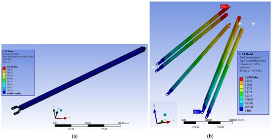
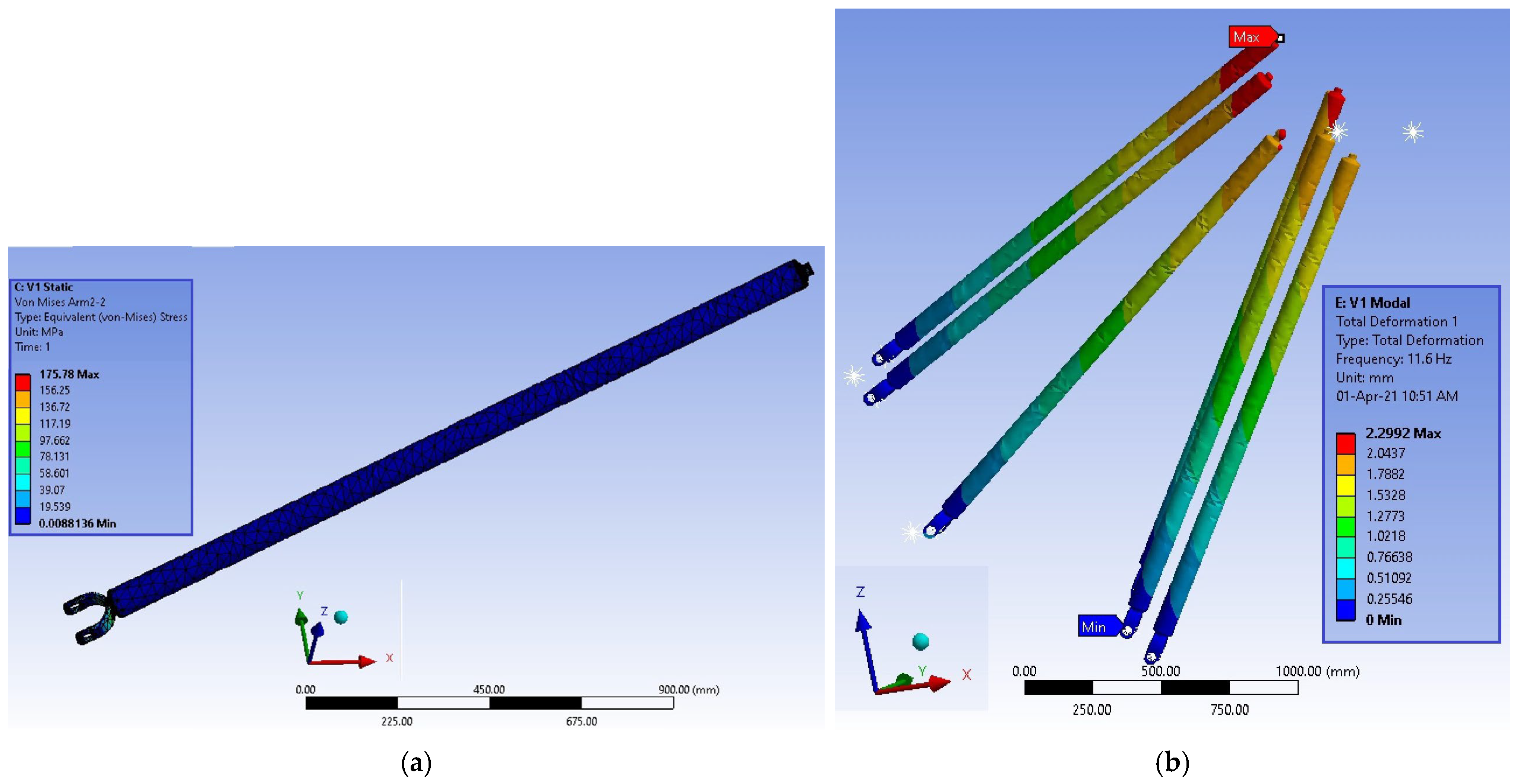
Figure 10 presents FEA results, as an example, for pose A in case WLX.

Figure 10. Pose A—case WLX. (a) von Mises stress of rod 2 of link 2, (b) modal analysis.

Figure 10a depicts the von Mises stress in one of the links of the assembly. It is observed that a very low average value is maintained throughout, while the maximum of about 130 MPa is located at the connection points with the respective joints. These local peaks are mainly associated with boundary-condition effects and modelling simplifications, since the joints are represented only by kinematic degrees of freedom and are not evaluated from a strength perspective. Therefore, stress values near the joint interfaces are interpreted qualitatively, whereas the stress distribution along the main body of the rod is considered representative for structural assessment. Even if maximum stresses observed are unrealistically high due to the simplifications adopted in modelling, they still remain well below the material yield limit; the main focus of the static analysis is on the calculated displacements.

Figure 10b shows the results of the natural frequency analysis.

Analogous results appear in all poses and cases, and Table 3 sums them up.

Table 3. Static analysis results for the original configuration for 6 end-effector coordinates.

Property	Case
	WLZ						WLX
	Pose
	A	B	C	D	E	F	A	B	C	D	E	F
Max von Mises Stress—Rods (MPa)	10	40	30	30	30	20	130	120	60	50	50	30
Max Reaction Force—Bases (kN)	25.0	43.9	62.9	61.5	61.5	23.7	111.4	129.0	78.5	65.0	65.0	46.0
Max Reaction Moment—Bases (kNm)	6.5	28.8	69.5	51.0	51.0	15.0	102.0	91.0	43.0	33.8	33.7	18.3
Max Reaction Force—Clamping System (kN)	17.0	17.0	26.0	27.8	27.8	18.8	52.9	39.0	29.4	21.2	21.2	75.0
Max Reaction Moment—Clamping System (kNm)	11.5	2.58	26.0	14.9	14.9	2.0	54.9	2.1	15.3	14.1	14.1	39.4
Axial Relative Displacement—Tool (mm)	−0.4	−0.2	−0.1	−0.2	−0.2	0.0	−5.6	−10.4	1.8	−0.4	−0.4	−0.2
Side Relative Displacement—Tool (mm)	1.4	−0.5	−0.9	−0.9	−0.9	−0.5	45.4	89.3	−4.0	−0.3	−0.3	3.5
First Mode (Hz)	11.6	17.1	9.7	10.7	10.7	8.0	2.1	1.8	18.0	24.2	24.2	5.0

Regarding maximum von Mises stress on links, since the yield stress of 1.2738 steel (DIN) is 900 MPa, there are no concerns associated with any of the poses. Regarding the reactions at the bases, both forces and moments are considered excessive (case WLZ) or even formidable (case WLX). As far as reactions in the clamping system are concerned, both forces and moments seem manageable, except for case WLX, where a very high force value of 75 kN is shown. Note that the bases and the clamping system can be made of many individual components that, if appropriately dimensioned, can collectively manage the required loads studied in separate FEA, which is outside the purpose of this study.

Regarding the relative displacement of the end-effector, results are satisfactory for case WLZ, as the largest displacement is barely 1.4 mm. However, in case WLX, the largest deviations exceed 10 mm.

As far as the first eigenfrequency is concerned, this is lower than 50 Hz in all poses, which hints at possible resonance in case of high rotary speeds of the spindle. Better performance is observed at the inner points of the workspace. In general, case WLX leads to much worse performance, mainly due to low stiffness.

Note that the increase in the workspace has led to small distances among the bases and, at the same time, to proportionally very long links. This configuration makes the distribution and possible mutual partial cancelling out of the developing forces and moments problematic. Thus, it is worth conducting a corresponding investigation into a modified arrangement to increase robustness at the expense of the workspace.

6. Tau-Robot Modified Configuration

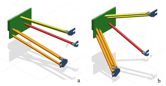
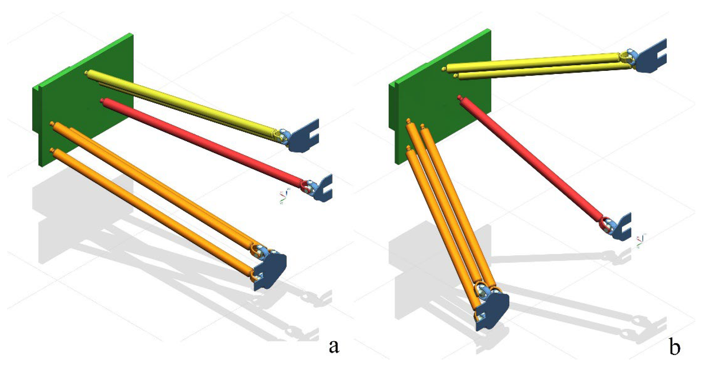
The new modified configuration has larger distances between the bases and decreased length of the links compared to the original, i.e., from 2 down to 1.5 m; see Figure 11.

Figure 11. Original configuration (a) versus modified (b) configuration.

A comparison of the dimensionless parameters with those of the original configuration is presented in Table 4. As for the angles of the geometric vectors $\left(\overrightarrow{Gi},\widehat{y}\right)$, the comparison is presented only for completeness, as the new global coordinate system has been placed at a different, more favourable point, with orientation still being maintained.

Table 4. Comparison of dimensionless parameters between initial and modified configurations.

Quantity	Initial	Modified
$\mathrm{angles} \left(\overrightarrow{Gi},\widehat{y}\right)$	{70,75,−83}	$\left\{\mathrm{29,96,6.5}\right\}$
mi	{60,8,3}	{7.1,1.2,1.4}
cis	{2,2,2}	{1.5,1.5,1.5}

Referring to Table 4, a very significant reduction is observed in the size factors (m_i) compared to the reduction in the length factors (c_is). Consequently, the size factors do not owe their large change to the new length of the links, but mainly to the enlargement of the layout, which has led to a greater contribution of the $\overrightarrow{Gi}$ vectors.

Figure 9b presents the new (dimensionless) workspace and the new points studied, their coordinate being given in Table 5. The new dimensions and geometric proportions of the layout lead to a very significant reduction in the workspace by 92% (from v₀ ≃ 5 to v_wide ≃ 0.8). Therefore, case WLX becomes necessary to exploit the $x^$-axis.

Table 5. Workspace points studied in the modified configuration.

End-Effector Vector	Points
	A	B	C	D	E	F
Rx  (mm)	1150.0	1320.0	2004.0	1104.0	1650.0	1450.0
Ry  (mm)	500.0	280.0	346.7	357.8	300.0	500.0
Rz  (mm)	1150.0	50.0	512.3	683.4	500.0	700.0

Static Analysis Results for the Modified Configuration

Table 6 presents the results for the two welding cases of the modified configuration. At first glance, a reduction in the loads is indeed observed for both cases in the modified configuration compared to the initial one. Again, case WLX is more demanding than case WLZ; however, the loads are now much more manageable than in the initial configuration. An additional improvement is also shown in the first natural frequency for both cases, which is due to the reduction in the length of the links, yet it is again marginally unsuitable regarding the 50 Hz limit.

Table 6. Static analysis results of the modified robot configuration for 6 end-effector coordinates and associated robot poses.

Property	Workspace Points
	Case WLZ						Case WLX
	A	B	C	D	E	F	A	B	C	D	E	F
Max von Mises—Rods (MPa)	10	10	10	10	10	10	10	20	40	30	30	30
Max Reaction Force—Bases (kN)	9.2	10.2	10.5	10.9	11.1	8.7	15.3	23.6	45.5	34.9	36.7	27.2
Max Reaction Moment—Bases (kNm)	13.1	11.1	6.8	7.4	5.4	11.7	21.9	35.4	65.2	49.6	52.7	38.5
Max Reaction Force—Clamping System (kN)	18.4	15.9	15.1	15.2	15.1	15.5	22.9	47.0	50.9	53.7	21.5	36.9
Max Reaction Moment—Clamping System (kNm)	8.1	1.1	4.1	5.0	4.0	5.2	9.8	13.9	21.2	23.6	8.1	14.4
Axial Relative Displacement—Tool (mm)	0.0	0.0	0.0	0.0	0.0	0.0	−0.1	−0.1	−0.2	−0.1	−0.2	−0.1
Side Relative Displacement—Tool (mm)	0.0	−0.0	−0.0	−0.0	−0.0	−0.0	−0.1	−0.1	−0.2	−0.5	−0.3	−0.0
First Mode (Hz)	33.9	53.0	44.5	42.0	46.0	37.5	54.5	35.7	27.8	38.9	23.7	53.0

Table 7 presents the comparison of the best, worst and mean values between the initial and the modified configuration for both cases. There is indeed an improvement in the modified configuration, as all load values show a decrease on average. The relative displacement is within the desired accuracy, even in case WLX, which confirms the increase in stiffness. The main frequency is significantly higher compared to the initial one, yet exceeding only in some cases the limit of 50 Hz. Thus, further reduction in the length of the links and introduction of damping elements are necessary.

Table 7. Configuration comparison (Org: original optimized, Mod: modified).

Properties	Case WLZ							Case WLX
	Best		Worst		Mean			Best		Worst		Mean
	Org	Mod	Org	Mod	Org	Mod	%	Org	Mod	Org	Mod	Org	Mod	%
Max von Mises (MPa) —Rods	10 (A)	10 (A)	40 (B)	10 (C)	30	10	76	30 (F)	10 (A)	130 (A)	40 (C)	70	30	60
Max Reaction Force (kN) —Bases	23.7 (F)	8.7 (F)	62.9 (C)	11.1 (E)	46.4	10.1	78	46.0 (F)	15.3 (A)	129.0 (B)	45.5 (C)	82.5	30.5	63
Max Reaction Moment (kNm) —Bases	6.5 (A)	7.4 (D)	69.5 (C)	13.1 (A)	36.9	9.3	75	18.3 (F)	21.9 (A)	102.0 (A)	65.2 (C)	53.6	43.9	18
Max Reaction Force (kN) —Clamping System	17.0 (A/B)	15.1 (C/E)	27.8 (D/E)	18.4 (A)	22.4	15.9	29	21.1 (D/E)	21.5 (E)	75.0 (F)	53.7 (D)	39.8	38.8	2
Max Reaction Moment (kNm) —Clamping System	2.0 (F)	1.1 (B)	26.0 (C)	8.1 (A)	11.9	4.6	62	2.1 (B)	8.1 (E)	54.9 (A)	23.6 (D)	23.3	15.2	35
Axial Relative Displacement (mm) —Tool	0.0 (F)	0.0	−0.4 (A)	0.0	−0.2	0.0	100	−0.2 (F)	−0.1 (F)	−10.4 (B)	−0.2 (E)	−2.5	−0.1	96
Side Relative Displacement (mm) —Tool	−0.5 (F)	−0.0 (B)	1.4 (A)	0.0 (A)	−0.4	−0.0	100	−0.3 (D/E)	−0.0 (F)	89.3 (B)	−0.5 (D)	22.3	−0.2	99
First Mode (Hz)	17.1 (B)	53.0 (B)	8.0 (F)	33.9 (A)	11.3	42.8	-	24.2 (D/E)	54.5 (A)	1.8 (B)	23.7 (E)	12.6	38.9	-

7. Discussion

The dimensionless model essentially serves to capture and increase the workspace. For the study of rigidity, it is obvious that different scales, i.e., values of Q, affect mass distribution, hence rigidity and natural frequencies. This is the reason why the relevant study was done for Q = 1 m, as a practical engineering choice to generate a realistic robot size compatible with commercially available components and typical FSW workspaces. For this reason, too, a modified configuration is subsequently investigated with shorter robot links and larger base spacing to restore stiffness and improve modal performance while sacrificing workspace, demonstrating that structural performance is governed primarily by dimensional scaling rather than the dimensionless optimization itself.

Although the modified configuration increases the first eigenfrequency, some poses still yield values close to the nominal spindle excitation frequency (~50 Hz at 3000 rpm). Therefore, resonance cannot be excluded solely by comparing eigenfrequencies, although damping at joints has not been modelled. In practice, vibration risk can be mitigated by (i) further stiffness-oriented tuning (shorter links, higher bending stiffness cross-sections, and increased joint stiffness), (ii) introducing damping at joints and/or at the spindle/end-effector interfaces to reduce resonance amplification, and (iii) planning the welding operations appropriately, i.e., selecting spindle speed ranges that avoid modal frequencies for the specific pose as well as trajectory/pose planning.

The robot configuration studied can indeed meet the requirements of FSW, especially by introducing a closed control loop, since the open loop performance is satisfactory. Note that the study was conducted for maximum loads corresponding to aluminum alloys. Consequently, the robot is expected to be capable of welding aluminum and other ductile materials such as brass alloys, mild steels and polymers.

Furthermore, by introducing linear guides in two independent links, the extension to 5 DoFs can be achieved, providing control for both tool and welding angles. Moreover, since this is a small range of angle change, short-stroke linear actuators are sufficient. This observation, in combination with the mean stress in the rods in the modified model, points to feasible solutions based on commercially available components.

Regarding the base supports, these can be improved by increasing the distances between the linear carriers or by reducing the length of the links, at the expense of the workspace. Linear carriers are widely used in practice involving high loads, as in this case. Furthermore, solutions can be designed that combine multiple carriages capable of compensating for lateral loads and overturning moments.

Modifications are made interactively to increase rigidity, starting from the kinematically optimum configuration that is universally applicable since it is dimensionless. Thus, the designer can introduce geometry modifications at will, which will reduce, of course, the workspace. Such a reduction may impact the size of the sheets, notably when the welding line is along the Z direction (case WLZ). Consequently, welding in the X direction seems indispensable.

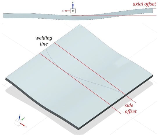
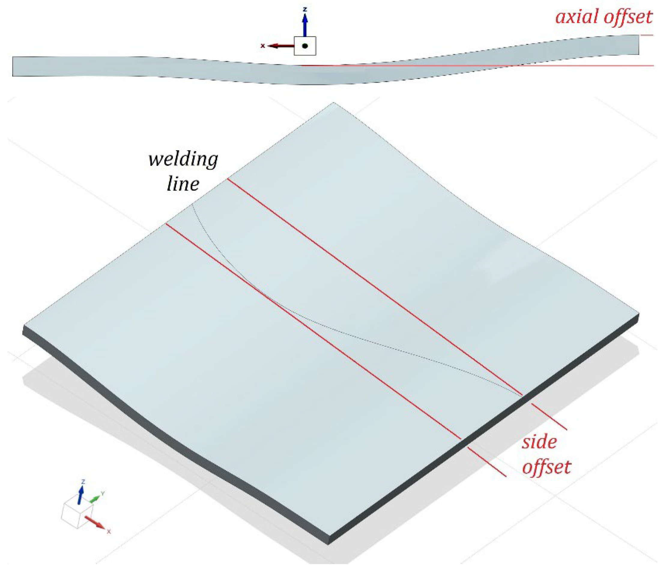
Figure 12 shows an FSW example of two sheets with a non-flat welding line in the X direction. Thus, the robot workspace must suffice to cover the displacement range in the two other directions, i.e., the side and axial offsets. In the modified configuration, the maximum side offset is about 720 mm, whereas the maximum axial offset is about 810 mm. By comparison, in the original optimized configuration, the offsets would be 2800 mm and 2100 mm, respectively. These dimensions are extracted from the workspace as the largest straight line segments in Y and Z that can be drawn continuously between two points within the workspace. As for the X-axis, it can potentially cover a distance of typically up to 2m, depending on the availability of reliable robot components.

Figure 12. Sheet metal parts to be welded, showing side and axial offsets.

Regarding the implementation potential for such a robot, first, linear slides with appropriate carriages are a standard, commercially available solution. For the extension to 5 DoFs, short-stroke hydraulic actuators with high resistance to lateral loads can be used, their use probably requiring additional bases for proper support. A significant challenge is the implementation of the joints. U-Joints that are available on the market are mainly aimed at power transmission, and they cannot handle lateral bending loads. Ideally, a cross-shaped U-Joint should be used.

8. Conclusions

In this work, significant steps were taken to investigate the kinematics, the workspace and the robustness of the Tau-robot, thereby clarifying its suitability for FSW, which is a very demanding manufacturing application in terms of loads on the robot.

The robustness can be practically increased interactively by constraining the distances of the bases as well as reducing the length of the links, i.e., practically by reducing the workspace, starting from the kinematically ideal situation determined first and serving as the baseline.

To exploit the configuration as much as possible, the welding line should be parallel to the linear guides of the device base.

In cases of relatively small welding lines, the Tau-robot is capable of providing a robust and reliable solution, given that the accuracy already achieved from the open loop is sufficient. The limitation of the dimensions of workpieces to be welded refers to the so-called offsets of the welding line and not to the workpiece dimensions, as the robot moves with respect to the welding line and not to the rest of the part’s surface. The welding line is approximately aligned with the X-axis of the global coordinate system.

In the future, we aim to investigate closed-loop control for the Tau-robot and test it on a suitable prototype, initially at a smaller scale in order to prove the concept. In addition, a new optimization exercise might be introduced to balance mechanical strength, vibration immunity and workspace. Since a number of computational tools will be needed in such an exercise, one of the implementation challenges would be to integrate them on the same optimization platform.

References

- Kaygusuz, E.; Karaomerlioglu, F.; Akinci, S. A review of friction stir welding parameters, process and application fields. Turk. J. Eng. 2023, 7, 286–295. [Google Scholar] [CrossRef] [Scilit]
- Kilic, S.; Ozturk, F.; Demirdogen, M.F. A comprehensive literature review on friction stir welding: Process parameters, joint integrity, and mechanical properties. J. Eng. Res. 2025, 13, 122–130. [Google Scholar] [CrossRef] [Scilit]
- Rai, R.; De, A.; Bhadeshia, H.K.D.H.; DebRoy, T. Review: Friction stir welding tools. Sci. Technol. Weld. Join. 2011, 16, 325–342. [Google Scholar] [CrossRef] [Scilit]
- Cook, G.E.; Crawford, R.; Clark, D.E.; Strauss, A.M. Robotic friction stir welding. Ind. Robot 2004, 31, 55–63. [Google Scholar] [CrossRef] [Scilit]
- Yue, W.; Liu, H.; Huang, T. An approach for predicting stiffness of a 5-DoF hybrid robot for friction stir welding. Mech. Mach. Theory 2022, 175, 104941. [Google Scholar] [CrossRef] [Scilit]
- Cheng, B.; Dong, B.; Chen, S.; Xiao, J. Effect of process parameters during the insertion phase of robotic friction stir welding on axial force. Int. J. Adv. Manuf. Technol. 2025, 137, 951–963. [Google Scholar] [CrossRef] [Scilit]
- Ibannai, A.I. Review of common defects in friction stir welding. Int. J. Sci. Technol. Res. 2020, 9, 318–329. [Google Scholar]
- Guillo, M.; Dubourg, L. Impact and improvement of tool deviation in friction stir welding: Weld quality and real-time compensation on an industrial robot. Robot. Comput.-Integr. Manuf. 2016, 39, 22–31. [Google Scholar] [CrossRef] [Scilit]
- Taghirad, H.D. Parallel Robots: Mechanics and Control; CRC Press: Boca Raton, FL, USA, 2025. [Google Scholar]
- Mo, S.; Hu, Y.; Huang, T.; Yao, B.; Chen, S.; Huang, Y.; Zhang, W. Dynamic modeling and performance analysis of a new friction stir welding parallel robot. Mech. Mach. Theory 2025, 210, 106030. [Google Scholar] [CrossRef] [Scilit]
- Zhao, J.; Duan, Y.; Xie, B.; Zhang, Z. FSW robot system dimensional optimization and trajectory planning based on soft stiffness indices. J. Manuf. Process. 2021, 63, 88–97. [Google Scholar] [CrossRef] [Scilit]
- Chai, X.; Zhang, N.; He, L.; Li, Q.; Ye, W. Kinematic sensitivity analysis and dimensional synthesis of a redundantly actuated parallel robot for friction stir welding. Chin. J. Mech. Eng. 2020, 33, 1. [Google Scholar] [CrossRef] [Scilit]
- Luo, H.; Zhao, F.; Guo, S.; Yu, C.; Liu, G.; Wu, T. Mechanical performance of friction stir welding robots for aerospace applications. Int. J. Adv. Robot. Syst. 2021, 18, 1729881421996543. [Google Scholar] [CrossRef] [Scilit]
- Luo, H.; Wu, T.; Fu, J.; Zhao, F. Analysis of typical working conditions and experimental research of friction stir welding robot for aerospace applications. Proc. Inst. Mech. Eng. Part C J. Mech. Eng. Sci. 2021, 235, 1045–1056. [Google Scholar]
- Sun, T.; Wu, H.; Lian, B.; Qi, Y.; Wang, P.; Song, Y. Stiffness modeling, analysis and evaluation of a 5-DoF hybrid manipulator for friction stir welding. Proc. Inst. Mech. Eng. Part C J. Mech. Eng. Sci. 2017, 231, 4441–4456. [Google Scholar] [CrossRef] [Scilit]
- Mousavi, S.; Gagnol, V.; Bouzgarrou, B.C.; Ray, P. Model-based stability prediction of a machining robot. Mech. Mach. Sci. 2017, 46, 379–387. [Google Scholar]
- Chalak Qazani, M.R.; Pedrammehr, S.; Abdi, H.; Nahavandi, S. Performance evaluation and calibration of Gantry-Tau parallel mechanism. Iran. J. Sci. Technol. Trans. Mech. Eng. 2020, 44, 1013–1027. [Google Scholar] [CrossRef] [Scilit]
- Akbari, M.; Esfandiar, M.; Abdollahzadeh, A. Role of force and torque in friction stir welding: A detailed review. J. Adv. Join. Process. 2025, 11, 100289. [Google Scholar] [CrossRef] [Scilit]
- Prabhakar, D.A.P.; Korgal, A.; Shettigar, A.K.; Herbert, M.A.; Chandrashekharappa, M.P.G.; Pimenov, D.Y.; Giasin, K. Review of optimization and measurement techniques of the friction stir welding process. J. Manuf. Mater. Process. 2023, 7, 181. [Google Scholar] [CrossRef] [Scilit]
- Yan, W.; Yu, Y. Study on force/position hybrid control strategy for eight-axis robotic friction stir welding. Metals 2025, 15, 442. [Google Scholar]
- Walz, D.; Sommer, K.; Werz, M.; Weihe, S. Development and evaluation of a robot-guided friction stir welding gun. Int. J. Precis. Eng. Manuf.-Green Technol. 2025, 12, 1795–1808. [Google Scholar] [CrossRef] [Scilit]
- Kolegain, K.; Leonard, F.; Zimmer-Chevret, S.; Attar, A.B.; Abba, G. Feedforward deflection compensation coupled with offline path planning for robotic friction stir welding. IFAC-PapersOnLine 2018, 51, 728–733. [Google Scholar] [CrossRef] [Scilit]
- Chen, S.; Zong, G.; Kang, C.; Jiang, X. Digital twin virtual welding approach for robotic friction stir welding based on FEA–robot co-simulation. Sensors 2024, 24, 1001. [Google Scholar]
- Zong, G.; Kang, C.; Chen, S.; Jiang, X. Optimization of installation position for complex space-curve weldments in robotic friction stir welding using dynamic dual particle swarm optimization. Processes 2024, 12, 536. [Google Scholar] [CrossRef] [Scilit]
- Patel, V.; Wouters, H.; Baghdadchi, A.; De Backer, J.; Igestrand, M.; Azimi, S.; Andersson, J. Robotic friction stir welding in lightweight battery assembly of extrusion-cast aluminum alloys. J. Adv. Join. Process. 2023, 8, 100156. [Google Scholar] [CrossRef] [Scilit]
- Silva-Magalhaes, A.; Cederqvist, L.; De Backer, J.; Håkansson, E.; Ossiansson, B.; Bolmsjö, G. Friction stir welding case study using temperature-controlled robotics with HPDC cylinder blocks and dissimilar materials. J. Manuf. Process. 2019, 46, 177–184. [Google Scholar] [CrossRef] [Scilit]
- Jin, T.; Cui, X.; Qi, C.; Yang, X. Development of a nonrigid-support friction stir welding repair robot for aluminum alloy trains. Ind. Robot 2024, 51, 490–500. [Google Scholar] [CrossRef] [Scilit]
- Raghulapadu, J.K.; Peddieson, J.; Buchanan, G.R.; Nunes, A.C. Rotating plug model of friction stir welding heat transfer. Heat Transf. Eng. 2008, 29, 321–327. [Google Scholar] [CrossRef] [Scilit]
- Ikumapayi, O.M.; Akinlabi, E.T.; Majumdar, J.D. Review on thermal, thermo-mechanical, and thermal stress distribution during friction stir welding. Int. J. Mech. Eng. Technol. 2018, 9, 534–548. [Google Scholar]
- Christy, J.V.; Mourad, A.H.I.; Sherif, M.M.; Shivamurthy, B. Recent trends in friction stir welding of aluminum alloys and aluminum matrix composites. Trans. Nonferrous Met. Soc. China 2021, 31, 3281–3309. [Google Scholar] [CrossRef] [Scilit]
- Takahara, H.; Motoyama, Y.; Tsujikawa, M.; Oki, S.; Chung, S.W.; Higashi, K. Allowance of deviation and gap in butt joints during friction stir welding. Adv. Mater. Res. 2007, 15–17, 375–380. [Google Scholar]
- Zimmer-Chevret, S.; Jemal, N.; Langlois, L.; Ben Attar, A.; Hatsch, J.; Abba, G.; Bigot, R. FSW process tolerance according to tool position and orientation: Requirements for production system design. Mater. Sci. Forum 2014, 783–786, 1820–1825. [Google Scholar] [CrossRef] [Scilit]
- Arian, A.; Danaei, B.; Abdi, H.; Nahavandi, S. Kinematic and dynamic analysis of the Gantry-Tau 3-DoF translational parallel manipulator. Appl. Math. Model. 2017, 51, 217–231. [Google Scholar] [CrossRef] [Scilit]
Disclaimer/Publisher’s Note: The statements, opinions and data contained in all publications are solely those of the individual author(s) and contributor(s) and not of MDPI and/or the editor(s). MDPI and/or the editor(s) disclaim responsibility for any injury to people or property resulting from any ideas, methods, instructions or products referred to in the content. |
© 2026 by the authors. Licensee MDPI, Basel, Switzerland. This article is an open access article distributed under the terms and conditions of the Creative Commons Attribution (CC BY) license.