


Abstract
This study presents a numerical framework for offline three-objective hole-sequence planning for an AC dual-rotary-head five-axis system. A double-curvature surface containing 48 staggered holes is used as a numerical case. For each hole, one representative inverse-kinematic branch is fixed, and the visitation permutation is the sole decision variable. The objectives minimize cumulative non-cutting tool-center-point (TCP) distance, cumulative A/C-axis adjustment, and estimated synchronized repositioning time. NSGA-II and NSGA-III are compared in 30 paired runs under identical computational settings. NSGA-II provides better median hypervolume and cross-fitted IGD+ and, relative to serpentine scanning, its compromise sequence reduces the three objectives by 6.631%, 56.254%, and 36.939%, respectively. Nearest-neighbor sequencing reduces TCP distance but increases rotary adjustment and estimated time. Diagnostics examine acceleration-aware timing, objective-count effects, selection preferences, inverse-kinematic branch choices, initial/return states, and finite C-axis windows. The results show that geometric proximity alone does not represent five-axis repositioning cost and that the time objective depends on relative axis-speed and dynamic assumptions. The reported improvements are numerical predictions for the synthetic geometry and virtual parameters; machine-specific post-processing, collision verification, digital-twin simulation, and dry-run validation remain necessary before industrial deployment.
1. Introduction
Multi-hole drilling on complex surfaces is widely encountered in the assembly and manufacturing of aerospace structural components. In aerospace manufacturing, five-axis orientation planning has been widely applied to complex components such as open blisks [1]. In such complex five-axis operations, smooth and feasible tool orientations are essential for maintaining machining performance [2]. Unlike planar multi-hole machining, holes on curved surfaces differ not only in spatial position but also in hole-axis direction, which varies with the local surface normal. Consequently, TCP translation and rotary-axis orientation adjustment generally occur simultaneously during inter-hole transfer on five-axis equipment. As the number of holes increases, the machining sequence directly affects non-cutting motion and inter-hole repositioning efficiency.
Existing studies on multi-hole drilling paths commonly formulate hole-sequence planning as a traveling salesman problem (TSP) or an extension thereof, with the primary objective of reducing inter-hole travel distance. Dewil et al. noted that sequence-dependent time, process constraints, and non-distance transfer costs remain important issues for further investigation in multi-hole drilling path optimization [3]. Genetic-algorithm-based approaches have been applied to optimize multi-hole drilling sequences by reducing non-cutting travel distance [4], while research on automatic drilling and riveting in aerospace manufacturing has demonstrated that operation-sequence planning involves trade-offs among efficiency, process constraints, and manufacturing requirements [5]. However, for five-axis drilling on complex surfaces, evaluating transfer cost solely by the Euclidean distance between holes cannot fully represent the motion characteristics of the five-axis machine tool.
Each hole on a complex surface is characterized by both its spatial position and axis orientation, and the hole-axis direction is generally determined by the local surface normal; therefore, positioning and orientation must be considered jointly [6,7,8]. Two holes that are close in Euclidean space may still have significantly different local surface normals, resulting in substantial A/C-axis orientation adjustment. Studies on free-form surface machining have demonstrated that geometric tool paths, Cartesian-space trajectories, and actual machine-axis motions represent different but interconnected planning levels [9]. Similar geometry-driven orientation planning strategies have been widely investigated in five-axis free-form surface machining [10]. Moreover, optimization of tool orientations and workpiece setups has been demonstrated to influence rotary-axis motion behavior and overall kinematic performance in five-axis machining systems [11]. Rotary-axis motion is affected by the machine kinematic chain, tool-length offset, rotation-center location, and RTCP implementation [12], while singularity handling and equivalent-angle treatment depend strongly on the specific five-axis configuration [13]. Thus, hole-sequence planning on complex surfaces must describe both spatial-position changes and rotary-orientation changes. However, existing sequence optimization studies mainly focus on discrete hole ordering, while the coupling relationship between hole sequence, tool orientation variation, and machine-axis repositioning cost remains insufficiently quantified for five-axis complex-surface drilling. Related five-axis machining studies have also emphasized that orientation planning should consider kinematic constraints and machining performance rather than geometric proximity alone [14].
Inter-hole repositioning time likewise cannot be represented simply by TCP distance or cumulative rotation angle. When multiple linear and rotary axes move synchronously, the transfer time of a segment is determined by the axis requiring the longest motion time, and the dominant axis may change from one inter-hole transfer to another. Consequently, optimizing only spatial distance may increase orientation adjustment, whereas optimizing only cumulative rotation may lead to longer spatial travel. Incorporating position, orientation, and time costs into a unified hole-sequence evaluation provides a more complete description of inter-hole transfer characteristics in five-axis drilling on complex surfaces.
Previous studies have addressed multi-hole drilling path optimization, multi-objective drilling and riveting sequence planning, curved-surface drill-axis positioning, and five-axis tool-orientation optimization from complementary perspectives [3,4,5,6,11]. Nevertheless, these research streams concern different planning levels. Conventional multi-hole-sequence studies mainly formulate discrete visitation order using point coordinates, travel distance, precedence constraints, or process-efficiency measures [3,4,5], whereas curved-surface and five-axis studies primarily focus on drill-axis orientation, tool pose, workpiece setup, or continuous machine-axis behavior [6,11]. Consequently, the explicit coupling of discrete hole visitation with curved-surface target poses and sequence-dependent translational, rotary, and synchronized-time costs remains insufficiently addressed. The methodological position of the present study relative to representative previous work is summarized in Table 1.
Table 1.
Comparison of representative related studies and the present numerical framework.
Recent studies have further advanced machine-aware planning for complex-surface manufacturing. Kong et al. developed drilling task planning and offline programming for robotic multi-spindle drilling of aero-engine nacelle acoustic liners, integrating normal-vector-based pose planning with drilling-path optimization [15]. Zhang et al. investigated kinematic-performance-oriented tool-orientation optimization for five-axis hybrid machining [16], while Wu et al. proposed collision-free tool-orientation smoothing based on safe attitude corridors and kinematic constraints [17]. Zaragoza Chichell et al. further investigated the simultaneous optimization of tool paths and local tool positioning for five-axis machining of free-form surfaces [18]. In addition, recent time-optimal feedrate-scheduling research has explicitly incorporated higher-order kinematic constraints for complex-surface robotic machining [19]. These developments demonstrate increasing attention to pose, kinematics, collision avoidance, and execution-time modeling; however, they address continuous toolpath or robotic-motion planning rather than the present fixed-branch discrete hole-sequence problem with simultaneous TCP-distance, A/C-adjustment, and synchronized-time objectives.
Based on these considerations, this study develops an offline hole-sequence planning method for complex-surface multi-hole tasks with known hole-entry centers, hole-axis directions, and hole depths. The method integrates surface geometry, single-hole process states, AC dual-rotary-head kinematics, and inter-hole transfer costs. To prevent inverse-kinematic branch selection from confounding the algorithm comparison, a representative A/C orientation independent of visitation order is fixed for each hole before optimization according to a deterministic rule, and the hole visitation permutation is used as the sole decision variable. The objectives are cumulative non-cutting TCP travel distance, cumulative A/C-axis adjustment, and estimated synchronized repositioning time.
The three-objective problem is solved using NSGA-II and NSGA-III with identical permutation encoding, initial populations, genetic operators, and function-evaluation budgets [20,21]. This work does not focus on modifying the multi-objective algorithms themselves; instead, the two algorithms, which use different selection mechanisms, are employed under a unified problem definition and computational setting to evaluate the effectiveness of the proposed three-objective hole-sequence model. Validation is performed using serpentine scanning and nearest-neighbor baselines, HV, IGD+, and nonparametric statistical tests.
The methodological contribution of this study does not lie in modifying NSGA-II or NSGA-III, but in formulating and integrating a five-axis hole-sequence planning problem that links curved-surface geometry, discrete target poses, and sequence-dependent motion costs. The main contributions are as follows. First, a geometry-to-pose mapping is established from the hole-entry position and local surface normal to the AC dual-rotary-head target orientation and the approach–entry–feed–retract process states, thereby introducing orientation information into discrete multi-hole planning. Second, a position–orientation–time three-objective permutation model is formulated by jointly minimizing cumulative non-cutting TCP distance, cumulative A/C-axis adjustment, and estimated synchronized repositioning time. By fixing one representative inverse-kinematic branch for each hole before optimization, the visitation permutation remains the sole decision variable and the sequence-level effects can be evaluated independently of branch encoding. Third, the resulting model is evaluated through deterministic baselines, 30 paired NSGA-II/NSGA-III runs under an identical computational budget, HV and IGD+ set-quality indicators, paired statistical tests, an independent-reference IGD+ audit, and supplementary objective-count, geometry, virtual-speed, acceleration, preference/compromise-selection, small-case IK-branch, initial/return-state, and finite-C-axis sensitivity analyses. The resulting framework therefore bridges curved-surface pose generation and discrete hole-sequence optimization without claiming modification of the underlying multi-objective evolutionary algorithms.
2. Materials and Methods
This study considers offline planning for five-axis multi-hole drilling on complex surfaces when the hole-entry centers, hole-axis directions, and hole depths are known. Conventional multi-hole drilling commonly uses Euclidean distance to formulate a TSP or its extensions, mainly to reduce idle travel and auxiliary time [3,4]; studies of automatic drilling and riveting in aerospace manufacturing also indicate multi-objective trade-offs between efficiency and other process objectives [5]. For complex-surface tasks, each hole additionally contains orientation information determined by the local surface normal [6]. Accordingly, the present method first generates hole positions and hole-axis directions from surface geometry, establishes an idealized AC dual-rotary-head kinematic model and fixes a representative inverse-kinematic branch, and then uses the hole visitation permutation as the sole decision variable. NSGA-II and NSGA-III are applied to solve a three-objective problem involving distance, A/C adjustment, and estimated repositioning time, and the results are evaluated using unified set-quality indicators and paired statistical tests.
2.1. Problem Definition and Overall Framework
2.1.1. Coordinate Systems and Five-Axis Target State
The machine coordinate system is denoted by {M}, the workpiece-coordinate system by {W}, and the tool coordinate system by {T}. The homogeneous transformation matrix of the workpiece-coordinate system relative to the machine coordinate system is expressed as
where is the rotation matrix of the workpiece-coordinate system relative to the machine coordinate system, and is the position of the workpiece-coordinate origin in the machine coordinate system.
For the kth hole, the hole-entry center and unit outward normal are transformed from the workpiece-coordinate system to the machine coordinate system according to
The position transformation includes both rotation and translation, whereas the direction-vector transformation includes rotation only. After coordinate transformation, the coordinate-system superscripts are omitted for conciseness, and and are used throughout the remainder of the paper.
The nominal five-axis target state of the kth hole is written as
where denotes the nominal TCP target position, and and denote the target angles of the AC dual-rotary head. Equation (3) does not represent the actual X/Y/Z/A/C machine-axis commands. The actual linear-axis commands are additionally affected by the rotation-center offset, tool length, setup transformation, and RTCP compensation strategy. This distinction is consistent with general five-axis workpiece-setup formulations [22].
2.1.2. Inputs, Outputs, and Scope of the Study
Let the total number of holes be N. The geometric and process data of the kth hole are expressed as
where is the hole-entry center, is the unit normal pointing outward from the workpiece, is the hole depth, and and are the approach and retract distances, respectively.
Other model inputs include the following:
The setup transformation from the workpiece-coordinate system to the machine coordinate system; the virtual initial and return states ; the allowable A-axis angular range and C-axis periodicity rule; the virtual rapid-traverse speeds of the X/Y/Z/A/C axes; and the population size, crossover probability, mutation probability, number of generations, and random seeds for NSGA-II and NSGA-III.
The model outputs include the hole-entry positions, hole-axis directions, approach–feed–retract process states, fixed representative A/C orientations, hole visitation sequence, three-objective nondominated solution set, and the complete discrete five-axis target-state sequence expanded along the selected hole sequence.
To avoid interpreting the nominal numerical model as an actual machine-control model, the scope and assumptions listed in Table 2 are adopted.
Table 2.
Main assumptions and scope of the nominal model.
2.1.3. Overall Computational Procedure
The workflow obtains hole centers and outward normals from a parametric surface or registered CAD, solves and verifies feasible AC inverse solutions, fixes one branch per hole, and generates the approach-entry-feed-retract states. Precomputed inter-hole TCP, rotary, and time costs are then used by NSGA-II and NSGA-III to optimize the same visitation-permutation problem; the resulting nondominated sets are evaluated consistently and a representative compromise is selected.
2.2. Generation of Surface Hole Positions and Single-Hole Process States
2.2.1. Parametric Surface and Unit Outward Normal
The outer surface of the component to be drilled is represented by a general parametric surface:
where Ω is the valid parametric domain of the surface.
The tangent vectors in the two parametric directions are
When and are linearly independent, the unit surface normal is expressed as
where σ ∈ {−1, 1} is used to enforce a consistent normal direction so that all normals point outward from the workpiece.
If the parametric coordinates of the kth hole are , the hole-entry center and outward hole-axis direction are, respectively,
Data preprocessing sequentially checks whether the parametric coordinates lie within the valid domain, whether the normal vectors are normalized, whether the normal directions are consistent, whether the hole depth is positive, and whether the subsequent process points lie within the prescribed virtual TCP range. These checks depend only on the geometry of each individual hole and do not change with the visitation sequence.
2.2.2. Tool Axis and Drilling Feed Direction
The outward tool axis is defined from the tool tip toward the spindle, while the drilling feed direction is defined from outside the workpiece toward its interior. Under ideal normal drilling, they satisfy
where is the target tool axis and is the drilling feed direction.
Therefore, the tool axis obtained from the forward kinematics of the AC dual-rotary head should be aligned with , while the motion from the approach point to the entry point and from the entry point to the feed-end point is along −.
2.2.3. Approach–Feed–Retract Process Points
The approach point, hole-entry point, feed-end point, and retract point of the kth hole are defined as
The superscripts a, e, f, and r denote approach, entry, feed end, and retract, respectively. The single-hole process-state sequence is
The approach and feed segments move along , whereas the retract segment moves along . The A/C orientation remains unchanged within each hole.
When , the approach and retract points have identical spatial coordinates but correspond to different discrete process states before and after drilling; therefore, both are retained in the complete state sequence.
Linear geometric interpolation is used between adjacent process points. If the start and end points of a local motion segment are and , respectively, then
Equation (13) describes only the geometric path and does not include controller interpolation cycles, velocity planning, acceleration, or jerk constraints. In free-form surface machining, geometric paths, Cartesian-space feed planning, and machine-axis trajectories are related but distinct planning levels.
2.3. AC Dual-Rotary-Head Kinematics and Fixed Representative Branch
2.3.1. Forward Kinematic Model
In this study, the C axis rotates about the fixed machine Z axis, while the A axis rotates about the local X axis after it has been carried by the C-axis rotation. The two elementary rotation matrices are
The combined rotation matrix is
When A = C = 0, the outward tool axis at the zero orientation is
The target tool-axis direction is therefore
Equation (17) applies only to the AC-axis order, positive directions, and zero orientation defined in this study. If an actual machine uses a different rotary-axis nesting relationship or positive direction, its kinematic model must be reconstructed accordingly. Trigonometric calculations are performed in radians, whereas angular results reported in the paper are converted to degrees. Five-axis accessibility and singularity-related constraints are highly dependent on the specific kinematic configuration of the machine tool [17].
2.3.2. Inverse-Kinematic Branches
Let the target outward normal of the kth hole be
and define its horizontal component as
When , two representative inverse solutions that produce the same tool-axis direction are
and
where is the threshold for detecting a directional singularity, and maps an angle to (−180°, 180°].
Based on the A-axis range and tool-axis directional error, the feasible branch set of the kth hole is defined as
where is the allowable numerical directional error. If is empty, the hole is unreachable under the current nominal configuration and angular range and should be reported before hole-sequence optimization.
2.3.3. Fixed Representative-Branch Rule
To ensure that NSGA-II and NSGA-III solve exactly the same permutation-optimization problem, the inverse-kinematic branch is not included as a genetic variable. Instead, one fixed representative branch is selected for each hole before sequence optimization.
The shortest-equivalent rotation between two C angles is defined as
The fixed representative branch of the kth hole is selected according to its normalized angular cost relative to the neutral orientation (A, C) = (0°, 0°):
The following definition is then used:
Equation (23) provides a visitation-order-independent orientation but does not minimize rotary motion for every sequence. Fixing the branches ensures that both algorithms evaluate identical permutations and objectives; their only algorithmic differences are the parent- and environmental-selection mechanisms.
When ρk ≤ εs, the tool axis approaches the machine Z axis, Ak = 0, and the C angle is directionally non-unique. To keep the representative orientation of every hole strictly independent of visitation order, the fixed rule Ak = 0° and Ck = C0 is used. The implementation sets εs = 10−12. In the main case, the minimum ρ is 0.019967 > εs, so none of the 48 holes triggers the singular branch. Every representative pose can therefore be fixed before optimization, and pairwise transfer costs can be precomputed statically. This rule is specific to the nominal AC configuration; an actual machine requires singularity handling consistent with its kinematic chain.
A post hoc small-case analysis is used to quantify the possible loss introduced by Equation (23). Sixteen holes are selected deterministically from rows 2–5 and columns 3–6 of the staggered grid (hole IDs 11–14, 19–22, 27–30, and 35–38). This central subset spans positive and negative A orientations and both signs of C while keeping exact branch enumeration and verification tractable. For every selected hole, both equivalent solutions in Equations (19) and (20) satisfy the nominal A-axis range and reproduce the same tool-axis direction.
Using random seed 20260929, 10,000 unique permutations of the 16 holes are generated. Each sequence is first evaluated with the fixed representative branches. Two sequence-dependent endpoint policies are then solved exactly by a two-state dynamic program whose state records the branch of the current hole and whose transitions include the initial and return home states. The rotation-optimal policy minimizes cumulative A/C adjustment Θ, with T as a deterministic tie-breaker; the time-optimal policy minimizes synchronized repositioning time T, with Θ as the tie-breaker. Cartesian target positions are unchanged by equivalent branch substitution, so D is identical among the three policies for a given sequence.
The fixed, rotation-optimal, and time-optimal objective triples are filtered separately in (D, Θ, T), and the two sequence-dependent endpoint sets are also pooled to form a branch-aware comparison front. Pareto-set sizes and sequence-identity retention are then compared. This diagnostic isolates the effect of branch assignment for sampled sequences; it is not a full joint evolutionary optimization of hole order and branch variables and does not enumerate every intermediate branch-related Pareto assignment.
2.3.4. Directional Error and Continuous-Angle Verification
Substituting the inverse solution back into Equation (17) gives the reconstructed tool axis . Its angular error relative to the target normal n_k is
This error is used to verify consistency between the analytical kinematic equations and the numerical implementation; it does not represent the orientation accuracy of an actual machine tool.
For a given visitation sequence, the continuous C-axis target angle is unwrapped segment by segment from the initial angle as follows:
Continuous unwrapping changes only the equivalent angular representation and does not alter the tool-axis direction corresponding to Equation (17).
Continuous unwrapping does not by itself guarantee compatibility with a finite-travel C axis. For an illustrative travel window [Cmin, Cmax], every principal target Ck is therefore expanded into the equivalent set {Ck + 360°l} that lies inside the window. If this set is empty for any hole, the sequence is declared infeasible under that window because a ±360° representation change cannot place the required target orientation inside the prescribed limits.
When all target sets are nonempty, a one-dimensional dynamic program selects the equivalent representation at every visited hole that minimizes cumulative absolute C-axis travel from the home angle C0 = 0° through the 48-hole sequence and back to C0. A change in the integer winding offset relative to the unbounded shortest-equivalent path is counted as a reindex/unwind event. The continuous baseline and symmetric windows of ±180°, ±120°, ±90°, and ±85° are examined. These windows are illustrative numerical conditions rather than certified limits or controller procedures for a specific machine tool.
2.4. Inter-Hole Transfer Model and Three Objective Functions
2.4.1. Hole Visitation Permutation and Transfer States
Define the hole visitation sequence as
subject to
Each hole must be visited exactly once. Define
where node 0 denotes the virtual initial and return state .
The TCP transfer displacement from node i to node j is defined as
Equation (29) consistently includes the transfer from the initial position to the first hole, transfers between adjacent holes, and the return from the final hole to the initial position. The current model checks only the geometric definition of discrete endpoints and straight-line segments; it does not include solid-body collision detection among the tool, rotary head, fixture, and workpiece.
2.4.2. Cumulative Non-Cutting TCP Travel Distance
The first objective is the cumulative Euclidean distance of all non-cutting TCP motion between holes:
This objective includes the motion from the initial position to the first hole, between adjacent holes, and from the final hole back to the initial position, but excludes the fixed approach, feed, and retract distances within individual holes.
denotes the nominal spatial travel distance of the TCP and is not equivalent to the cumulative X/Y/Z-axis travel of an actual machine under RTCP.
2.4.3. Cumulative A/C-Axis Adjustment
For transfer segment i → j, the A-axis and C-axis adjustments are defined as
The cumulative rotary-axis adjustment is
is measured in degrees. This objective quantifies the cumulative angular change between discrete target orientations and serves as a geometric proxy for rotary-axis motion; it does not directly represent motor energy consumption, drive load, vibration, or structural fatigue.
Equation (32) weights one degree of A and C motion equally as a geometric measure, not as equivalent actuator effort. A post hoc speed-normalized burden, Θv = Σ(|ΔAij|/vA + |ΔCij|/vC), therefore tests the available speed information without claiming an energy model. With vA = 30°/s and vC = 60°/s, one degree of A contributes twice one degree of C. Θv is a serial-equivalent rotary measure and differs from the synchronized maximum-component time T in Equation (33).
2.4.4. Estimated Synchronized Repositioning Time
Because actual axis acceleration, jerk, controller interpolation cycle, and look-ahead parameters are unavailable, constant virtual rapid-traverse speeds are used to construct an inter-hole repositioning-time surrogate model.
Let
Assuming that all five axes start and finish simultaneously, the estimated repositioning time from node i to node j is taken as the maximum of the independent motion times of the five axes:
where , , and are in mm/s, while and are in °/s.
The cumulative estimated synchronized repositioning time is
excludes approach, drilling feed, dwell, retract, tool change, chip evacuation, and inspection within each hole. It should therefore be interpreted only as the estimated synchronized inter-hole repositioning time and not as the complete drilling cycle time.
Because Equation (33) uses a maximum-component operator, the transfer time may be governed by any linear or rotary axis. Consequently, is not a fixed linear combination of and .
2.4.5. Three-Objective Permutation-Optimization Model
Combining the above objectives, the sequence-optimization model for multi-hole drilling on complex surfaces is formulated as
subject to the following constraints:
If the actual C axis has a finite travel range, a travel constraint should additionally be imposed on the continuous absolute angle obtained from Equation (26). In the numerical case study, the C axis is treated as an ideal continuous-rotation axis.
2.5. Solution Methods: NSGA-II and NSGA-III
NSGA-II and NSGA-III are Pareto evolutionary algorithms that use nondominated sorting but different diversity mechanisms: crowding distance in NSGA-II and reference-direction niching in NSGA-III [20,21]. They are used here as unmodified alternative solvers for the same three-objective permutation problem under an identical function-evaluation budget.
2.5.1. Permutation Encoding and Initial Population
Because a representative A/C orientation is fixed for every hole before optimization, the chromosome contains only the hole visitation permutation:
Each hole index therefore occurs exactly once, and no inverse-kinematic branch gene is included. The initial population contains random feasible permutations together with the serpentine-scanning and nearest-neighbor sequences, which provide two deterministic engineering baselines while the random individuals maintain population diversity. For each paired trial, NSGA-II and NSGA-III use the same initial population and random-seed index.
2.5.2. Crossover and Mutation
Order crossover is employed for recombination, and segment-reversal mutation is used to modify local visitation order. Both operators preserve the permutation structure so that every hole appears exactly once and no duplicate-hole repair is required. The segment-reversal operation can be expressed as
The crossover and mutation probabilities are identical for NSGA-II and NSGA-III and are reported together with the remaining algorithm parameters in Section 3.1.1.
2.5.3. NSGA-II Environmental Selection
NSGA-II ranks candidates by nondomination level and crowding distance [20]. Parent tournaments use these two criteria, and environmental selection admits successive fronts; crowding distance resolves truncation of the last admissible front.
2.5.4. NSGA-III Environmental Selection
NSGA-III retains nondominated sorting but uses reference-direction association and niching for the last admissible front [21]. Parent tournaments compare ranks, with a random resolution of equal-rank ties.
For M objectives and a single-layer Das–Dennis division parameter H, the number of reference directions is
In this study, M = 3 and H = 12, giving 91 reference directions; the population size is 92 to retain the adopted two-parent/two-offspring implementation. Although NSGA-III was originally developed with many-objective optimization in mind, its performance on the present three-objective permutation problem is assessed empirically under the same computational budget as NSGA-II rather than assumed a priori.
2.5.5. Termination Criterion and Repeated Runs
Both algorithms terminate after the same fixed maximum number of generations, and nondominated sets and quality indicators are recorded at identical checkpoints. Multiple independent paired runs are performed to reduce the influence of stochastic variation; runs with the same seed index share the same initial population and random state. Statistical comparisons are based on the final nondominated set of each individual run. The union of solutions across repeated runs is used to visualize the candidate objective region, construct the pooled empirical reference front, and select representative compromise solutions, rather than as the statistical unit. A separate cross-fitted reference construction, defined in Section 2.6.4, is used to verify that the IGD+ comparison is not driven by inclusion of the evaluated run in its own reference front. The detailed population size, generation limit, number of paired runs, and random seeds are reported in Section 3.1.1.
2.6. Evaluation of Nondominated Solution Sets and Compromise-Solution Selection
2.6.1. Aggregated Empirical Front
The final population of each run is subjected to nondominated filtering to obtain the final nondominated set for that run. The results from repeated runs of the same algorithm are then combined, and duplicate objective vectors and numerically dominated solutions are removed to form an algorithm-level aggregated front.
The final nondominated solutions from all NSGA-II and NSGA-III runs are subsequently combined and filtered again to obtain the pooled empirical reference front Rpool. This front is an empirical approximation obtained under the current algorithms, computational budget, and case-study conditions and is not equivalent to the unknown theoretical Pareto front.
2.6.2. Selection of a Compromise Solution
A common empirical ideal point and empirical worst point are first determined from the combined final empirical reference front of NSGA-II and NSGA-III. For the rth candidate on the aggregated front Sa of algorithm a, the mth objective is range-normalized using these common bounds:
where zm* and zmnad are, respectively, the minimum and maximum of the mth objective on the combined empirical reference front and are identical for NSGA-II and NSGA-III.
If an objective does not vary on the combined empirical reference front, its normalized value is set to zero. For each algorithm, the Euclidean distance of a candidate in Sa from the common normalized ideal point (0, 0, 0) is
The representative compromise solution of each algorithm is
Common normalization makes the compromise scales comparable, after which one representative is selected within each algorithm’s aggregated front. This decision rule does not imply simultaneous global minimization of all objectives.
To evaluate whether the reported representative solution depends on decision preferences or the compromise-selection rule, a post hoc sensitivity analysis is performed on the 223-point aggregated NSGA-II front. NSGA-II is used because the paired set-quality analysis and the cross-fitted IGD+ audit favor its front under the present computational setting. No optimization is rerun, and the analysis changes only the decision layer applied after nondominated solutions have been obtained.
Three preference scenarios are considered. The equal scenario retains (D, Θ, T) with weights (1/3, 1/3, 1/3), thereby reproducing the published no-prior-preference selection. The speed-normalized scenario replaces Θ by Θv and applies equal criterion weights to (D, Θv, T); the transformed union of the NSGA-II and NSGA-III fronts is refiltered, and common empirical ideal and nadir bounds are recomputed before selecting from the transformed NSGA-II nondominated subset. The time-priority scenario retains (D, Θ, T) but assigns weights (0.2, 0.2, 0.6). The latter weights are illustrative rather than elicited from a specific manufacturer.
Each scenario is evaluated by three deterministic rules. The weighted ideal-point rule minimizes weighted normalized distance; TOPSIS maximizes closeness to the weighted anti-ideal point; and the knee rule selects the largest ideal-directed distance from the plane through the three single-objective extremes. These rules test sensitivity to preference weights, rotary scaling, and compromise geometry without claiming to cover all industrial policies.
2.6.3. Unified Normalization and HV
Algorithm set-quality evaluation uses unified normalization bounds that are independent of the compromise-solution selection. Let the unified minimum and maximum of the mth objective over all algorithms and saved checkpoints be and , respectively. Then
Let S denote the nondominated set after unified normalization, and let the HV reference point be
The three-objective HV is then defined as
where denotes the three-dimensional Lebesgue measure. Under the same normalization bounds and reference point, a larger HV indicates a larger dominated volume and better coverage of the nondominated set relative to the adopted empirical bounds. Because HV is sensitive to the reference point, all algorithms must use exactly the same normalization and reference point [23].
2.6.4. Pooled and Cross-Fitted IGD+ Evaluation
Let Rpool be the pooled empirical reference front and S the normalized nondominated set obtained from one algorithm run. The pooled-reference IGD+ used in the primary set-quality comparison and indicator-evolution curves is defined as
where
A smaller IGD+ indicates that the nondominated set obtained by the algorithm is closer to the empirical reference front and provides better coverage. Compared with conventional IGD, IGD+ accounts for dominance in the distance calculation and has improved Pareto compliance [24].
Because Rpool contains nondominated points from all runs, the pooled-reference value may benefit from including points contributed by the evaluated run. An evaluation-independent audit is therefore performed by deterministic two-fold cross-fitting. The 30 matched run indices are divided into fold A (odd RunIDs) and fold B (even RunIDs), giving 15 paired runs per fold. For a run in fold A, the reference front is the nondominated union of final solutions from both algorithms in fold B; for a run in fold B, the reference front is formed analogously from fold A. Thus, neither the evaluated run nor its same-index algorithm counterpart contributes to the reference front, while both algorithms in each matched pair are evaluated against exactly the same complementary-fold front.
2.6.5. Paired Statistical Tests
HV and IGD+ are compared between matched seed indices using two-sided Wilcoxon signed-rank tests [25], with Holm correction across the two indicators to control the family-wise error rate [26].
In addition to the adjusted p values, the paired rank-biserial correlation coefficient is reported:
where W+ and W− are the positive and negative rank sums. Differences are defined as NSGA-III minus NSGA-II for HV and NSGA-II minus NSGA-III for IGD+; positive differences favor NSGA-III, whereas negative rank-biserial correlations favor NSGA-II.
The statistical conclusions apply only to the present case study, algorithm settings, and function-evaluation budget and are not intended to establish universal superiority of one algorithm for all three-objective or multi-objective problems.
2.6.6. Late-Stage Changes and Runtime
To avoid interpreting late-stage stability solely from the visual appearance of the indicator-evolution curves, the relative changes in HV and are examined over the final iteration interval. For any indicator Q, the late-stage change rate is defined as
Predetermined thresholds are applied to the absolute late-stage changes in both HV and IGD+. Satisfying them is described only as small late-stage change and does not demonstrate convergence to the theoretical Pareto front.
Runtime is compared only on the same computer, MATLAB version, and program implementation, and the median over repeated runs is reported. The result is not extrapolated to other hardware, programming languages, or parallel implementations.
2.7. Baseline Methods and Validation Protocol
2.7.1. Serpentine-Scanning Baseline
Serpentine scanning visits holes row by row, with adjacent rows traversed in opposite directions. The path is regular but does not use surface-normal or A/C-orientation information. Its fixed representative orientations, initial/return states, and objective functions are exactly the same as those used by the optimization algorithms.
2.7.2. Nearest-Neighbor Baseline
Starting from the virtual initial position, the nearest-neighbor method repeatedly selects, from the unmachined holes, the hole closest to the current retract point:
where is the set of holes that have not yet been visited. When the current position is the virtual initial point, is replaced by .
Nearest neighbor uses only TCP Euclidean distance, excluding A/C angles and time, and therefore tests whether shorter spatial travel implies lower five-axis cost. The two baselines are deterministic and are excluded from stochastic significance tests.
2.7.3. Geometric and Kinematic Validation
Geometric validation includes the following checks:
- whether the surface parametric coordinates lie within the valid domain;
- whether the magnitude of each unit normal is close to 1;
- whether all normals consistently point outward from the workpiece;
- whether the hole depth, approach distance, and retract distance satisfy the prescribed values; and
- whether the process states are generated in the order approach–entry–feed end–retract.
The back-substitution errors of the approach distance, hole depth, and retract distance are defined as
Kinematic validation checks whether the fixed representative A/C angles lie within the virtual axis ranges, whether the tool axis reconstructed by forward kinematics agrees with the target hole axis, and whether the continuous C-axis representation contains unnecessary full-revolution jumps.
The above errors are used to verify program self-consistency and must not be interpreted as actual machine-tool positioning error, tool-axis perpendicularity error, or drilled-hole depth accuracy.
2.7.4. Validation of the Complete Discrete State Sequence
The complete operation sequence consists of the virtual initial state, four process states for each hole, and the return state. The total number of discrete states is
The TCP coordinates, A-axis angles, and continuous C-axis angles in the complete sequence are checked individually against the prescribed virtual ranges. The maximum inter-hole TCP distance, maximum A-axis increment, maximum shortest-equivalent C-axis increment, and maximum estimated repositioning time are also recorded. The numerical validation and algorithm-evaluation protocol is summarized in Table 3.
Table 3.
Numerical validation and algorithm-evaluation protocol.
2.8. Objective Correlation and Virtual-Speed Sensitivity Evaluation
The three-objective hole-sequence model uses non-cutting TCP travel distance D, cumulative A/C-axis adjustment Θ, and estimated synchronized repositioning time T. The value of T is obtained by summing, segment by segment, the maximum of the times corresponding to the five motion components in Equation (33). It is therefore affected by both the hole visitation sequence and the virtual linear- and rotary-axis speed settings. To determine whether the three metrics contain substantial information redundancy, whether T changes the retained trade-off set, and whether the main optimization trend depends excessively on one speed combination, objective-correlation, objective-count, and speed-parameter sensitivity analyses are performed.
For the objective-correlation analysis, while keeping the geometry of the main case study, the fixed representative A/C inverse-kinematic branches, and the initial/return states unchanged, L = 10,000 complete visitation sequences are randomly generated from the 48-hole permutation space. D, Θ, and T are calculated for each sequence. Because the relationships among the objectives may be nonlinear but monotonic, Spearman’s rank correlation coefficient is used to evaluate the association between each pair of objectives [27]. For variables X and Y, the Spearman correlation coefficient is defined as
A value of closer to 1 indicates a more similar ranking relationship between the two metrics; however, a high correlation does not by itself imply that the objectives are mathematically equivalent or equivalent under all parameter settings. Therefore, this study also compares changes in the correlation structure under different virtual-speed conditions rather than deciding whether an objective should be removed on the basis of a single correlation coefficient.
The same 10,000 sequences are also used for a two-versus-three-objective diagnostic. Let S2 denote the nondominated subset obtained by minimizing only D and Θ, and let S3 denote the nondominated subset obtained by minimizing D, Θ, and T. The two sets are constructed independently under V1, V2, and V3. Every member of S2 remains nondominated in three dimensions for the present samples, whereas S3 may retain additional sequences whose time advantage compensates for inferior D or Θ. The number of candidates retained in S3 but not S2 therefore measures the sampled trade-off alternatives introduced by the time objective.
For coverage comparison, all three objectives are range-normalized using the minimum and maximum values of the same 10,000-sequence pool in each speed scenario. The three-dimensional HV of S2 and S3 is calculated with the common normalized reference point (1.1, 1.1, 1.1), and the retained-HV ratio is HV(S2)/HV(S3). IGD+ is additionally computed using S3 as the empirical reference and S2 as the approximation set. These deterministic diagnostics quantify the incremental information provided by T within the sampled sequence space. They do not replace a separate two-objective optimization run and do not establish objective necessity for every machine-speed configuration.
For virtual-speed sensitivity, the speed combination used in the formal main case is taken as the reference scenario V1:
Two relative-speed variations are then considered. In V2, the linear-axis speeds remain unchanged while the A/C-axis speeds are increased to 60/120°/s, representing relatively faster rotary axes. In V3, the A/C-axis speeds remain unchanged while the X/Y/Z speeds are increased to 400/400/200 mm/s, representing relatively faster linear axes. Hole geometry, fixed representative inverse-kinematic branches, initial and return states, and all other model parameters are identical among the three scenarios.
V1 directly uses the reference-case results described above. V2 and V3 are supplementary sensitivity tests conducted with a reduced computational budget of 92 individuals, 3000 generations, and 10 paired random seeds; the crossover and mutation probabilities remain 0.90 and 0.20, respectively. These tests are intended to assess the stability of objective relationships and optimization trends under changes in relative axis speed. They do not replace the formal 30-run, 6000-generation statistical comparison in Section 3.3 and are not used to calibrate the axis dynamics of any actual machine tool.
2.9. Acceleration-Aware Post Hoc Evaluation of Repositioning Time
Equation (33) neglects axis acceleration. To assess whether this simplification affects the relative evaluation of candidate sequences, the hole sequences contained in the final nondominated sets of the 30 paired runs are reevaluated without changing the hole geometry, fixed inverse-kinematic branches, virtual initial and return states, or virtual-speed limits. After duplicate permutations are removed, 2337 unique sequences remain from 2981 recorded nondominated solutions. This is a post hoc sensitivity evaluation; the evolutionary optimization is not rerun using the acceleration-aware time.
For axis with displacement , virtual maximum speed , and assumed acceleration , the minimum rest-to-rest motion time is evaluated as when ; otherwise, a triangular profile is used with . For each transfer, the synchronized time is the maximum of the five-axis times, and the cumulative value is obtained over the 49 transfers, including the initial and return movements. The shortest-equivalent C-axis increment defined in Equation (25) is retained.
Three illustrative acceleration settings are considered. For the high-acceleration setting, X/Y/Z accelerations are 2000/2000/1000 mm/s2 and A/C accelerations are 300/600 °/s2. The corresponding values are 1000/1000/500 mm/s2 and 100/150 °/s2 for the medium setting, and 500/500/250 mm/s2 and 50/75 °/s2 for the low setting. These values are uncalibrated numerical assumptions rather than measured parameters of a project machine. Each transfer is treated as an independent stop-to-stop motion; jerk, controller look-ahead and interpolation, and RTCP-induced coupling of machine-axis trajectories are not included.
2.10. Initial/Return Safe-Point Post Hoc Sensitivity
The objective definitions include the auxiliary transfer from the initial state to the first-hole approach point and the return from the last-hole retract point. To isolate sensitivity to the location of the home, tool-change, or safe point, the reported NSGA-II representative sequence is therefore reevaluated under two illustrative alternatives while retaining all 47 inter-hole transfers, fixed inverse-kinematic branches, virtual axis speeds, and neutral rotary coordinates A0 = C0 = 0°. The high-clearance point pH = (0, −250, 200) mm changes only the nominal Z coordinate by +50 mm, whereas the right-side tool-change point pT = (300, −250, 150) mm changes only X by +300 mm. Both points lie within the prescribed virtual TCP ranges.
For each alternative, only the home-to-hole-4 approach transfer and the hole-5 retract-to-home transfer are recomputed using the same Euclidean-distance and synchronized maximum-component time definitions as the main analysis. The evolutionary optimization is not rerun. This design quantifies the endpoint contribution to the published representative route but does not estimate how the entire Pareto front would change if a different safe point were imposed before optimization.
3. Numerical Results and Validation
Numerical validation is performed on a double-curvature parametric surface containing 48 staggered holes. Surface geometry, single-hole process states, and AC dual-rotary-head kinematics are checked sequentially, and NSGA-II and NSGA-III are compared under a unified computational budget. In addition to the main case study, geometry-perturbation, objective-correlation, virtual-speed, acceleration-aware time-model, and initial/return-point sensitivity tests are used to examine the robustness and limits of the main conclusions. The machine-readable numerical data supporting the figures, tables, and post hoc sensitivity analyses are provided in Supplementary File S1.
3.1. Numerical Simulation Environment and Case-Study Setup
3.1.1. Computational Environment and Numerical Experimental Design
All programs were executed in MATLAB R2024b (24.2.0.2712019) under 64-bit Windows 11 Pro (version 25H2; OS build 26200.8875) on a computer equipped with a 12th Gen Intel Core i7-12700 CPU (2.10 GHz) and 16 GB RAM. The numerical case uses aligned workpiece and machine coordinate systems, i.e., an identity setup transformation. The virtual initial/return position is p0 = (0,−250,150) mm, with A0 = C0 = 0°. NSGA-II and NSGA-III use 30 one-to-one paired random seeds (20260720–20260749). Within each pair, the algorithms share the same initial population, initial random state, genetic operators, and function-evaluation budget to reduce the influence of random initialization.
The algorithms use the same encoding, initial populations, crossover and mutation operators, objectives, and evaluation budget. Differences are confined to their defined selection mechanisms: NSGA-II uses nondomination rank and crowding distance for parent and environmental selection; NSGA-III uses rank with random equal-rank parent ties and reference-direction association with niching for environmental selection. Suitability is evaluated directly through same-budget paired trials.
The principal simulation parameters are listed in Table 4.
Table 4.
Numerical case-study and algorithm parameters.
The axis ranges and speeds in Table 4 are numerical test parameters only. The third objective accumulates only the estimated synchronized repositioning time from the initial position, between holes, and back to the return position; it excludes in-hole machining and auxiliary operations. Therefore, the reported time-improvement rate must not be interpreted as an improvement in the complete drilling cycle time.
3.1.2. Double-Curvature Surface and Hole Distribution
Normal drilling of curved aerospace structures requires each hole to be described by both its spatial position and local surface-normal direction [6,28,29]. In an industrial workflow, these quantities can be obtained from registered CAD geometry or measurement data and then transferred to an offline planning layer. To isolate the position–orientation coupling investigated in this study and keep the test case fully reproducible without relying on proprietary production geometry, the present numerical case adopts a synthetic, non-proprietary double-curvature surface with a staggered hole group. The geometry shown in Figure 1 is therefore a controllable numerical surrogate rather than a reconstruction of a specific industrial component. It retains the two features required for the present investigation—spatial variation in hole centers and continuous variation in hole-axis directions—while allowing the geometric and kinematic inputs to be reproduced consistently. Machine-specific post-processing, RTCP compensation, solid-body collision checking, and NC verification remain outside the scope of the present numerical case study.
Figure 1.
Synthetic staggered hole distribution and unit outward normals on the double-curvature test surface.
The parametric equation is
where and are the surface parameters, and and are the equivalent transverse and longitudinal curvature radii of the skin, respectively.
The surface parametric ranges are set to
u ∈ [−250, 250] mm, v ∈ [−180, 180] mm.
The curvature radii are set to
Rx = 1200 mm, Ry = 2500 mm.
Let
Its partial derivatives with respect to the two parameters are
The two tangent vectors of the parametric surface are
The unit normal pointing outward from the surface is obtained from their cross product as
Six staggered rows of holes are arranged on the surface, with eight holes in each row. The parametric coordinates of the ith hole in the jth row are
where
The staggered offset for even-numbered rows is defined as
Accordingly, the hole-entry center of hole (i, j) is
The corresponding outward hole-axis direction is , and the drilling feed direction is . The resulting hole distribution and unit outward normals are shown in Figure 1.
The normal inclination gradually increases as the holes move from the central region toward the surface edges. Different holes therefore correspond to different TCP positions and A/C target orientations. The present work verifies only the mapping from geometry to discrete target poses and hole sequence; controller interpolation and actual axis dynamics are not simulated [9].
3.1.3. Single-Hole Process States
Each hole contains approach, entry, feed-end, and retract states. The uniform depth is 6 mm, and the approach and retract distances are 20 mm. States are generated from the entry center and outward normal; equal approach and retract distances produce coincident coordinates but distinct pre- and post-drilling states. Figure 2 shows holes 1, 24, and 48.
Figure 2.
Approach–feed–retract process states for representative holes: (a) Hole 1; (b) Hole 24; (c) Hole 48. A, E, F, and R denote the approach, entry, feed-end, and retract states, respectively.
These three holes are located in different regions of the surface, and their local hole-axis directions vary with the surface normal; nevertheless, each process segment remains aligned with its corresponding hole axis. This confirms that the proposed single-hole state-generation method automatically adapts to local surface geometry.
3.1.4. Inverse Kinematics of the AC Dual-Rotary Head and Fixed-Branch Rule
A/C orientations are obtained from Section 2.3 and fixed before optimization using Equation (23), subject to the A-axis range and directional-error tolerance. The visitation permutation is therefore the only decision variable. C is treated as continuous and adjacent moves use the shortest-equivalent rotation. This controlled formulation does not imply that the fixed branch minimizes rotary motion for every sequence [13].
3.1.5. Three-Objective Evaluation and Compromise-Solution Selection
The optimization minimizes D, Θ, and T as defined in Section 2.4, including the initial, inter-hole, and return transfers. Common bounds from the combined final nondominated solutions—ideal (2918.449889, 513.945408, 16.572854) and worst (3951.507444, 1467.349353, 28.326024)—normalize the objectives, and each algorithm’s representative is the point nearest the common normalized ideal. This selection is a reporting rule, not a claim of simultaneous global minima.
3.2. Geometric and Kinematic Validation
3.2.1. Validation of Hole Positions and Process States
All 48 holes lie within the prescribed surface parametric ranges, and all normal vectors are normalized. The inverse-kinematic direction-error tolerance is 1 × 10⁻⁵° and the singularity threshold is εs = 1 × 10⁻¹². The minimum ρ is 0.019967, so no singular branch is triggered. Numerical back-substitution for the approach distance, hole depth, and retract distance gives the following maximum errors:
These errors are at the level of double-precision floating-point roundoff, demonstrating consistency between the single-hole process-state relations defined in Section 2.2.3 and their numerical implementation.
3.2.2. A/C-Axis Angle Results
After applying the fixed representative-branch rule in Equation (23), feasible A/C angles are obtained for all 48 holes; the maximum tool-axis back-substitution error is below 1 × 10⁻⁵°, and no hole triggers the ρ ≤ εs singular branch. The resulting A-axis and principal C-axis angles for all holes are shown in Figure 3.
Figure 3.
A-axis angles and principal C-axis angles under the fixed representative-branch rule: (a) A-axis angles; (b) principal C-axis angles.
The A-axis angle range is
The principal C-axis angle range is
Substituting the selected A/C angles back into Equation (17), the maximum angular error between the reconstructed tool axis and the target hole axis is
The horizontal axis in Figure 3 represents the hole index rather than the optimized machining sequence. Therefore, angular differences between adjacent hole indices cannot be interpreted directly as actual inter-hole rotary-axis motion. The cumulative rotary motion for a given sequence can be obtained only after the A/C angles are reordered according to that visitation sequence and the shortest-equivalent rotations are calculated.
3.3. Multi-Objective Optimization Results
3.3.1. Pareto Fronts and Representative Solutions
After 30 independent runs, the final nondominated solutions from all runs of each algorithm are merged, and duplicate objective vectors and numerically dominated solutions are removed. The aggregated NSGA-II front contains 223 nondominated solutions, while the aggregated NSGA-III front contains 105. Combining the results from all runs of both algorithms yields an empirical reference front containing 233 objective vectors.
Aggregated fronts visualize repeated-run coverage and construct the pooled empirical reference set; statistical inference instead uses the 30 paired final-run sets. The complementary-fold audit excludes each evaluated pair from its reference, and Figure 4 shows the aggregated fronts and selected compromises.
Figure 4.
Three-objective Pareto fronts and compromise solutions of NSGA-II and NSGA-III.
The results reveal clear conflicts among travel distance, rotary-axis adjustment, and estimated time. The boundary solutions and compromise solutions of the two algorithms are listed in Table 5.
Table 5.
Representative solutions on the aggregated Pareto fronts.
For NSGA-II, the minimum-distance solution has D = 2918.450 mm, Θ = 1467.349°, and T = 28.326 s, whereas the minimum-rotation solution has Θ = 513.945° and D = 3951.507 mm. Thus, spatial proximity does not ensure orientation proximity [30], and the segment-wise maximum-component definition prevents T from being a fixed linear combination of D and Θ.
3.3.2. HV, IGD+, and Statistical Significance
To compare solution sets fairly, all objectives use common quality-evaluation bounds determined from every algorithm and saved checkpoint: zmin = (2918.449889, 513.945408, 16.572854) and zmax = (5197.882540, 1562.927912, 29.493297), in the objective order (D, Θ, T). The HV reference point is
For the normalized nondominated set S, HV is defined as the union volume of the region dominated by S and bounded by the reference point:
where λ(⋅) is the three-dimensional Lebesgue measure. Exact deterministic slicing is used. With common bounds and reference point, larger HV indicates greater dominated volume and coverage relative to the adopted empirical bounds [23].
Let Rpool denote the pooled empirical reference front. Pooled-reference IGD+ is defined as
where
A smaller pooled-reference IGD+ indicates that the obtained solution set is closer to the pooled empirical reference front and provides better coverage of it. Compared with conventional IGD, IGD+ improves Pareto compliance by modifying the distance calculation to account for dominance [24].
The distributions of HV and IGD+ over the 30 paired runs are shown in Figure 5, and the statistics are summarized in Table 6.
Figure 5.
Distributions of HV and pooled-reference IGD+ over 30 paired runs: (a) HV; (b) pooled-reference IGD+. The p values are Holm-adjusted, and |r| denotes the absolute paired rank-biserial correlation coefficient.
Table 6.
Set-quality indicators based on the pooled empirical reference front.
The median HV of NSGA-II is higher than that of NSGA-III, whereas its median IGD+ is lower, indicating that NSGA-II obtains final nondominated sets with better overall coverage quality for the present fixed-branch three-objective permutation problem.
Paired two-sided Wilcoxon tests compare the matched runs, and Holm correction controls the two-indicator family [25,26]. The results are summarized in Table 7.
Table 7.
Results of the primary paired statistical tests.
Differences are oriented so that positive values favor NSGA-III for both indicators. After Holm correction, both p values are below 0.05 with large absolute effect sizes, supporting better NSGA-II set quality for this case and budget.
To test reference-set independence, odd and even RunIDs are used as complementary folds. The front formed from the even runs contains 246 nondominated objective vectors and evaluates the odd runs; the front formed from the odd runs contains 291 vectors and evaluates the even runs. Table 8 summarizes the resulting cross-fitted IGD+ values. In every comparison, the evaluated run and its matched counterpart are absent from the reference front.
Table 8.
Evaluation-independent cross-fitted IGD+ over 30 paired runs.
Cross-fitted median IGD+ is 0.005091 for NSGA-II and 0.011624 for NSGA-III; 25 of 30 pairs favor NSGA-II. The exact paired test gives W = 38, p = 1.218 × 10⁻⁵, median difference −0.006261, and rank-biserial correlation −0.837. This independent-reference audit supports the primary comparison without self-inclusion.
This result is limited to the fixed-branch, 48-hole, three-objective case. It does not establish universal NSGA-II superiority because performance depends on objective count, front geometry, and problem structure [20,21].
3.3.3. Late-Stage Indicator Changes and Computational Time
The median evolution of HV and IGD+ over the 30 runs of both algorithms is shown in Figure 6.
Figure 6.
Median HV and pooled-reference IGD+ versus generation number: (a) median HV; (b) median pooled-reference IGD+.
During the early generations, HV increases rapidly and IGD+ decreases rapidly for both algorithms, indicating that the serpentine, nearest-neighbor, and random sequences in the initial population can quickly generate improved solutions through genetic operations. As evolution proceeds, the rates of change in both indicators gradually decrease.
To assess late-stage indicator behavior without treating the curves as proof of convergence, the final 10% of generations, i.e., generations 5400–6000, is used for an auxiliary assessment of changes in HV and pooled-reference IGD+. The results are given in Table 9.
Table 9.
Late-stage changes in the quality indicators.
The thresholds are 1% for absolute HV change and 5% for absolute pooled-reference IGD+ change. NSGA-II satisfies only the HV threshold because its IGD+ still decreases by 13.149%; NSGA-III satisfies both, although its indicators are not monotonic. The 6000-generation outputs are therefore empirical nondominated fronts under the specified budget, not evidence of theoretical convergence.
On the same computer and under the same MATLAB implementation, the median runtime per NSGA-II run is 5.597 s, compared with 10.233 s for NSGA-III; the latter is approximately 1.83 times longer. This difference primarily reflects the implementation overhead of crowding-distance selection versus reference-direction association in the present program and is not used to infer general runtime efficiency under other programming languages, hardware platforms, or problem scales.
3.4. Engineering Comparison of Different Machining Sequences
3.4.1. Spatial Visitation Paths
The spatial visitation paths of serpentine scanning, nearest neighbor, the NSGA-II compromise solution, and the NSGA-III compromise solution are shown in Figure 7.
Figure 7.
Inter-hole spatial transfer paths for four machining sequences: (a) serpentine scanning; (b) nearest neighbor; (c) NSGA-II compromise solution; (d) NSGA-III compromise solution.
Serpentine scanning follows regular alternating rows, whereas nearest neighbor shortens local TCP travel but ignores orientation. The two optimized paths instead group holes with smoother position-normal changes, so they are not reproductions of either baseline.
3.4.2. Objective Values and Improvement Rates
The objective values of the four sequences and their improvement rates relative to serpentine scanning are listed in Table 10 and compared graphically in Figure 8.
Table 10.
Objective values of different machining sequences.
Figure 8.
Comparison of the three objectives for four machining sequences: (a) non-cutting distance; (b) cumulative A/C-axis adjustment; (c) estimated repositioning time. Snake denotes serpentine scanning, and NN denotes nearest neighbor.
The improvement rate is defined as
A positive value indicates an objective reduction, whereas a negative value indicates an increase relative to serpentine scanning. Objective values in Table 10 and the text are rounded to three decimals; improvement rates and small pairwise differences are calculated from unrounded results.
The nearest-neighbor sequence reduces non-cutting distance by 2.245% but increases cumulative A/C adjustment by 8.380% and estimated time by 7.125%. This result directly demonstrates that simply selecting the spatially nearest hole may cause larger orientation changes. For drilling on complex surfaces, a conventional Euclidean-distance TSP cannot fully describe inter-hole transfer cost.
Compared with serpentine scanning, the NSGA-II compromise solution reduces distance, cumulative rotation, and estimated time by 6.631%, 56.254%, and 36.939%, respectively; the corresponding reductions for the NSGA-III compromise solution are 6.628%, 55.864%, and 37.016%. Compared with the nearest-neighbor sequence, the NSGA-II compromise solution reduces non-cutting TCP travel distance, cumulative A/C-axis adjustment, and estimated synchronized repositioning time by 4.487%, 59.636%, and 41.134%, respectively.
The two compromises are close: NSGA-III is 0.02055 s faster, whereas its distance and rotation are higher by 0.100 mm and 5.511°. These local differences do not determine algorithm performance; the HV, IGD+, and paired tests support using the aggregated NSGA-II representative for subsequent validation.
The three objective values of the representative NSGA-II compromise solution are 3042.005 mm, 619.599°, and 16.904 s, and its hole visitation sequence is
Selecting this route for state validation does not imply machine-level optimality; deployment should choose from the nondominated set using verified machine and production priorities.
3.5. Validation of the Complete Target-State Sequence and Motion Ranges
3.5.1. Complete TCP and A/C Sequences
The complete operation state sequence is expanded using the representative NSGA-II compromise hole sequence in Equation (76). The sequence consists of the virtual initial state, four process states for each of the 48 holes, and the return state, for a total of 1 + 48 × 4 + 1 = 194 discrete target states. The TCP coordinates and A/C-angle sequences for the NSGA-II compromise hole sequence are shown in Figure 9.
Figure 9.
TCP coordinates and AC dual-rotary-head angle sequence for the representative NSGA-II compromise hole sequence: (a) TCP coordinates; (b) A-axis and continuous C-axis angles.
Within each hole, the target A- and C-axis angles remain unchanged while the TCP passes successively through the approach point, entry point, feed-end point, and retract point. After the current hole is completed, the TCP and rotary axes transfer to the approach state of the next hole. Because the C axis uses the shortest-equivalent rotation and a continuous representation, the complete sequence contains no unnecessary full-revolution jump caused by switching across the ±180° principal-angle boundary.
3.5.2. Virtual Motion Ranges
The coordinate and angular ranges of the complete target-state sequence are listed in Table 11.
Table 11.
Target-state ranges for the representative NSGA-II compromise hole sequence.
All target states satisfy the virtual limits, but the TCP coordinates are nominal tool-tip positions rather than physical X/Y/Z commands. Real-axis travel depends on rotary-center offsets, tool length, setup, and RTCP implementation [12]; in a machine implementation, measurement-based adjustment can further modify target states [31]. The continuous C range is likewise a numerical result, with explicit finite-window checks reported in Section 3.5.5.
3.5.3. Adjacent-State Transfer Magnitudes
The representative NSGA-II compromise sequence contains 47 inter-hole transfers, together with two auxiliary transfers from the virtual initial position to the first hole and from the final hole back to the initial position. The maximum single-step transfer magnitudes are listed in Table 12.
Table 12.
Maximum single-step transfer magnitudes for the representative NSGA-II compromise sequence.
The maximum inter-hole TCP distance occurs in the transfer from hole 20 to hole 29 and is 87.834 mm, with a corresponding A-axis increment of 3.572°. The maximum shortest-equivalent C-axis rotation occurs from hole 37 to hole 44 and is 43.660°, corresponding to an estimated synchronized repositioning time of 0.728 s.
The longest TCP transfer and largest C increment occur on different moves, confirming that distance alone cannot represent five-axis transfer cost. Segment time is governed by the slowest normalized axis component and therefore depends on the linear-to-rotary speed ratio.
Including the endpoint states raises the maximum TCP move to 172.920 mm and maximum estimated time to 1.261 s. Endpoint definitions therefore affect cumulative results and must accompany route comparisons; Section 3.5.4 tests two alternatives.
3.5.4. Initial/Return Safe-Point Sensitivity
The released transition table reproduces the reported representative objectives with absolute discrepancies below 5 × 10⁻¹² in their respective units. Table 13 then substitutes the two alternative safe points defined in Section 2.10. Because all three safe states use A0 = C0 = 0° and the hole sequence is unchanged, cumulative A/C-axis adjustment remains 619.599° in every scenario; only D and T change.
Table 13.
Post hoc sensitivity of the representative NSGA-II route to the initial/return safe-point location.
Raising the safe point by 50 mm increases the two auxiliary distances and makes both transfers Z-axis limited, increasing total D by 2.590% and total T by 5.916%. Moving the safe point 300 mm in +X increases total D by 11.796%, but the resulting X-axis-limited transfers increase total T by only 3.286%. The larger distance change therefore does not produce the larger time change because synchronized repositioning time is governed by the slowest normalized axis component rather than by Euclidean distance alone.
The initial/return state is part of the objective definition. A production home, tool-change, or collision-free safe point should be specified in machine coordinates before optimization rather than substituted afterward.
3.5.5. Finite C-Axis Travel and Reindex/Unwind Check
The unbounded shortest-equivalent reconstruction exactly reproduces the released C-angle sequence, with a maximum discrepancy of 4.97 × 10⁻¹⁴°. The representative path occupies C ∈ [−86.277°, 85.967°], so the minimum centered symmetric half-range that contains every target is 86.277°. Its cumulative C-axis travel, including the home-to-first-hole and final-hole-to-home movements, is 532.522°.
Table 14 reports the finite-window check. The ±180°, ±120°, and ±90° windows are all feasible without changing the equivalent-angle winding index. Consequently, no reindex/unwind event is required, cumulative C travel remains 532.522°, and the estimated synchronized repositioning time remains 16.904 s. The ±90° case has the smallest positive margin, 3.723°, and should therefore be interpreted as a numerical boundary check rather than a recommended engineering allowance.
Table 14.
Finite C-axis window check for the representative NSGA-II compromise sequence.
Under the ±85° stress window, holes 17, 24, 25, and 32 exceed the travel limit, producing 16 infeasible target states and a minimum margin of −1.277°. Adding or subtracting 360° moves these targets farther outside the narrow symmetric window, so a reindex/unwind operation alone cannot restore feasibility. This case would require a different inverse-kinematic branch or machine setup, a wider C-axis range, or re-optimization with the finite travel constraint included explicitly.
3.6. Supplementary Robustness Validation Under Changed Geometric Conditions
The preceding numerical results are based on fixed double-curvature parameters and a regular staggered hole pattern. To examine whether the main conclusions of the joint position–orientation–time sequence optimization depend excessively on a single geometric condition, three additional geometric cases are considered while keeping the number of holes, single-hole process parameters, fixed representative inverse-kinematic branches, virtual axis speeds, initial/return states, and definitions of the three objectives unchanged.
Case A uses the same geometric conditions as the main case, namely and , and retains the original 6 × 8 staggered hole distribution as the reference case for the supplementary tests. In Case B, the curvature radii are reduced to = 900 mm and = 1800 mm. In Case B, the curvature radii are reduced to Rx = 900 mm and Ry = 1800 mm, increasing the variation in surface-normal orientation while leaving the number of holes and their parametric layout unchanged. In Case C, = 1200 mm and = 2500 mm are retained, but bounded deterministic perturbations are added to the original regular parametric hole coordinates. The maximum perturbation amplitudes in the u and v directions are 8 mm and 6 mm, respectively, to represent a hole pattern deviating from a regular array. The perturbations are generated by deterministic trigonometric functions and introduce no additional random geometric error; therefore, identical hole geometry is used in all repeated trials.
where and are both in millimeters. The perturbation contains no random variable; consequently, every repeated calculation uses exactly the same irregular hole geometry.
All 48 holes in each of the three cases pass the same orientation-feasibility and virtual-motion-range checks as the main case.
The purpose of this section is only to examine the sensitivity of the main optimization trend to geometric changes, rather than to repeat a formal statistical ranking of NSGA-II and NSGA-III. The supplementary tests therefore use a reduced computational budget: the population size remains 92, each algorithm is run for 3000 generations, and 10 paired random seeds are used; the crossover and mutation probabilities remain 0.90 and 0.20, respectively. Because the formal 30-run comparison in Section 3.3 showed that NSGA-II had better overall solution-set quality for the present fixed-branch three-objective problem, the compromise solution from the aggregated NSGA-II candidate set is compared mainly with the deterministic serpentine and nearest-neighbor baselines in this section.
The objective values for the different sequences under the three geometric conditions are listed in Table 15. Although Case A uses the same geometry as the main case, its stochastic optimization uses the reduced budget of 10 runs and 3000 generations. Consequently, the NSGA-II compromise solution differs slightly from the solution obtained in the formal 30-run, 6000-generation test in Section 3.4. The serpentine and nearest-neighbor baselines are deterministic and therefore remain identical to those of the main case. Case A serves only as a reference for Cases B and C under the same supplementary computational budget and does not replace the formal results in Section 3.3 and Section 3.4.
Table 15.
Supplementary hole-sequence optimization results under different geometric conditions.
Using the serpentine result of each case as the reference and the definition in Equation (75), the improvement rates are shown in Figure 10. In Case A, the NSGA-II compromise solution reduces non-cutting distance, cumulative A/C adjustment, and estimated repositioning time by 6.627%, 55.715%, and 37.200%, respectively. When the curvature is increased in Case B, the corresponding reductions remain 6.623%, 54.152%, and 36.289%. After deterministic perturbations are introduced into the regular hole pattern in Case C, the reductions are 7.284%, 51.395%, and 36.335%, respectively. Thus, under all three tested geometric conditions, the NSGA-II compromise solution simultaneously reduces the three objectives of positional motion, orientation adjustment, and the time surrogate, with broadly comparable improvement magnitudes.
Figure 10.
Objective improvement rates of nearest neighbor and the NSGA-II compromise solution relative to serpentine scanning under different geometric conditions: (a) non-cutting TCP travel distance; (b) cumulative A/C-axis adjustment; (c) estimated synchronized repositioning time. Case A denotes the reference geometry, Case B the increased-curvature condition, and Case C the irregular-hole condition. Positive values indicate objective reductions; negative values indicate increases.
In contrast, the nearest-neighbor method achieves only small distance reductions in all three cases. In Cases A and B, non-cutting distance decreases by 2.245% and 2.146%, respectively, whereas cumulative A/C adjustment increases by 8.380% and 8.352% and estimated repositioning time increases by 7.125% and 7.146%. This conflict becomes more pronounced in the irregular-hole Case C: although nearest neighbor reduces non-cutting distance by 1.512%, it increases cumulative A/C adjustment by 43.141% and estimated repositioning time by 35.072%. This indicates that, as the spatial regularity of the hole pattern decreases, selecting the next hole solely by TCP Euclidean distance is more likely to produce transfers between spatially close holes with large orientation changes.
Across the tested curvature and deterministic perturbations, spatial and orientation proximity remain distinct and the multi-objective route retains balanced improvements. Because all cases remain synthetic 48-hole tests with reduced budgets and improving indicators near generation 3000, their fronts are empirical and are not generalized to arbitrary parts or machines.
3.7. Objective Correlation, Objective-Count, and Virtual-Speed Sensitivity Analysis
3.7.1. Correlation Analysis of the Three Objectives
To analyze the statistical associations among the three hole-sequence objectives, 10,000 complete random hole sequences are generated from the 48-hole permutation space of the main case using a fixed random seed. For each sequence, the non-cutting TCP travel distance D, cumulative A/C-axis adjustment Θ, and estimated synchronized repositioning time T are calculated. Pairwise scatter plots for the three objectives under the reference speed V1 are shown in Figure 11, and the Spearman rank correlation coefficients under different speed scenarios are listed in Table 16.
Figure 11.
Objective correlations for 10,000 random hole sequences under the reference virtual speed V1: (a) non-cutting TCP travel distance versus cumulative A/C-axis adjustment; (b) non-cutting TCP travel distance versus estimated synchronized repositioning time; (c) cumulative A/C-axis adjustment versus estimated synchronized repositioning time. ρs denotes Spearman’s rank correlation coefficient.
Table 16.
Spearman rank correlation coefficients among the three objectives under different virtual-speed scenarios.
Under the reference speed V1, the Spearman correlation coefficient between D and Θ is only 0.0966, indicating almost no stable monotonic relationship between spatial travel distance and cumulative rotary-axis adjustment. This is consistent with the nearest-neighbor baseline: a sequence constructed using TCP Euclidean distance can reduce spatial travel without guaranteeing a simultaneous reduction in orientation change. The correlation coefficient between D and T is 0.3777, whereas that between Θ and T is 0.9080, showing that under the reference virtual-speed setting, estimated repositioning time is strongly associated with rotary motion but still cannot be described by spatial distance alone.
More importantly, the correlation structure between T and the other two objectives changes substantially with the relative speeds of the linear and rotary axes. When the A/C-axis speeds are doubled, the D-T correlation in V2 increases from 0.3777 to 0.7972, while the Θ-T correlation decreases from 0.9080 to 0.4968. This means that faster rotary motion reduces its contribution to the synchronized-transfer bottleneck, causing the time objective to depend relatively more on linear displacement. Conversely, when the linear-axis speeds are doubled, the D-T correlation in V3 decreases to 0.1809, while the Θ-T correlation increases to 0.9863, indicating that synchronized repositioning time is then governed mainly by rotary motion for most random sequences.
Thus, T cannot be replaced by a fixed D- or Θ-based surrogate: its ranking relationship changes with the speed ratio because Equation (33) selects a different dominant axis by segment. Retaining T captures this machine-dependent synchronization effect without claiming complete independence from the geometric objectives.
3.7.2. Two-Versus-Three-Objective Nondominated-Set Analysis
Table 17 compares the sampled nondominated sets formed with D and Θ alone (S2) and with D, Θ, and T (S3). The comparison uses identical sequence samples within each speed scenario. Point retention reports |S2|/|S3|, while the HV and IGD+ columns evaluate S2 in the full three-objective space relative to S3.
Table 17.
Two-versus-three-objective nondominated-set size and coverage for 10,000 random sequences.
Under V1, adding T increases the sampled nondominated set from 8 to 11 sequences. The two-objective set therefore retains 72.7% of the three-objective candidates and 99.462% of its three-dimensional HV, with an IGD+ of 0.003869. Under V2, S3 contains 12 sequences, including four that are excluded by the D–Θ comparison; S2 retains 66.7% of the candidates, 99.625% of HV, and has an IGD+ of 0.009796. The added candidates demonstrate that a sequence can be dominated in the two geometric motion totals but remain nondominated after its synchronized repositioning time is considered.
Under V3, S2 and S3 both contain the same eight sequences, so the retained-HV ratio is 100% and IGD+ is zero. This result is consistent with the very high Θ–T rank correlation of 0.9863 in V3: when linear axes are relatively fast, cumulative rotary motion closely tracks the segment-wise time bottleneck in this sample. The comparison therefore does not show that T is uniformly independent of D and Θ. Instead, it quantifies a speed-dependent contribution: T adds three or four distinct trade-off candidates under V1 and V2, but its incremental nondominated-set contribution disappears under V3. Because the HV gain is below 0.6% in V1 and V2, the main benefit in this random sample is additional trade-off diversity rather than a large expansion of dominated objective-space volume.
3.7.3. Sensitivity Analysis of Virtual Axis Speeds
Because the estimated synchronized repositioning time explicitly depends on the virtual speeds of the individual axes, supplementary comparisons are performed under the reference-speed scenario V1, the relatively faster rotary-axis scenario V2, and the relatively faster linear-axis scenario V3 to examine sensitivity to the speed settings. For any given hole sequence, changing the speed parameters does not alter its TCP geometric path or A/C target orientations; therefore, D and Θ remain unchanged. However, the frequency with which different axes become the synchronized-motion bottleneck changes, thereby altering T and the compromise sequence found by the multi-objective search.
The objective values of serpentine scanning, nearest neighbor, and the NSGA-II compromise solution under the three speed scenarios are listed in Table 18. V1 uses the reduced-budget reference result described above. Relative to serpentine scanning, the NSGA-II compromise solution reduces non-cutting distance, cumulative A/C adjustment, and estimated repositioning time by 6.627%, 55.715%, and 37.200%, respectively. After the A/C-axis speeds are doubled, the corresponding improvement rates for the V2 compromise solution are 6.896%, 54.795%, and 19.956%. The improvements in distance and cumulative orientation adjustment remain similar to those of the reference case; however, because rotary-axis motion time decreases substantially, the serpentine time itself drops from 26.806 s to 19.324 s, reducing the relative room for improvement in the time objective.
Table 18.
Hole-sequence optimization results under different virtual-speed conditions.
When the X/Y/Z linear-axis speeds are doubled while the A/C-axis speeds remain unchanged, the NSGA-II compromise solution in V3 improves distance, cumulative A/C adjustment, and estimated time by 6.111%, 56.456%, and 51.882%, respectively. Under this condition, the required linear-motion time decreases and rotary motion more readily becomes the synchronized-motion bottleneck. Consequently, the time advantage of optimized sequences with smaller cumulative orientation changes is amplified. This behavior is consistent with the high correlation ρs(Θ,T) = 0.9863 observed for V3 in Section 3.7.1.
The nearest-neighbor baseline further illustrates the same issue. Because this sequence is determined solely by TCP geometric distance, D and Θ remain unchanged across all three speed scenarios: the distance is always 2.245% lower than that of serpentine scanning, while cumulative A/C adjustment is always 8.380% higher. However, the deterioration in estimated time changes from 4.043% in V2 to 7.125% in V1 and further to 9.522% in V3. Thus, the same geometric sequence can have different time consequences under different linear-to-rotary axis speed ratios.
This comparison has a direct machine-selection implication. A nearest-neighbor order or a distance-only TSP tour has fixed geometry after it is generated, but it does not have a machine-independent time ranking: changing the linear-to-rotary speed ratio can change the dominant axis in Equation (33), the time assigned to each edge, and the representative Pareto solution. The inter-hole time matrix should therefore be rebuilt from the rated or measured capabilities of the target machine. Reusing only the shortest Cartesian tour is justified only when orientation changes are negligible or are verified not to control the segment times.
Overall, changing the virtual axis speeds clearly affects the absolute value of the third objective, the correlation structure among objectives, and the representative compromise solution, but it does not change the principal optimization conclusion within the tested range: reducing TCP distance alone may still increase orientation adjustment and synchronized repositioning time, whereas incorporating position, orientation, and time simultaneously in the Pareto evaluation produces more balanced hole sequences under different relative-speed conditions. This also confirms that T should be interpreted as a motion-time surrogate dependent on the axis-speed parameters, rather than as an equipment-independent intrinsic property of a hole sequence. For practical application, the time objective should be reevaluated using verified speeds of the target machine together with more detailed acceleration, jerk, and controller-kinematic parameters.
The corresponding objective improvement rates under the three virtual-speed scenarios are shown in Figure 12.
Figure 12.
Objective improvement rates of nearest neighbor and the NSGA-II compromise solution relative to serpentine scanning under different virtual-axis speed scenarios: (a) non-cutting TCP travel distance; (b) cumulative A/C-axis adjustment; (c) estimated synchronized repositioning time. V1 is the reference speed; V2 doubles the A/C-axis speeds; V3 doubles the X/Y/Z-axis speeds. Positive values indicate objective reductions, whereas negative values indicate increases.
It should be noted that V2 and V3 use the reduced computational budget of 10 runs and 3000 generations. Over the final 10% of generations, the median HV of NSGA-II changes by approximately 0.209% and 0.190% in V2 and V3, respectively, while IGD+ still decreases by approximately 14.44% and 23.26%. Therefore, the supplementary cases do not simultaneously satisfy all late-stage stability thresholds used in the formal main experiment. The results in this section are used only to evaluate objective relationships and major optimization trends under changed speed parameters. They are interpreted as empirical nondominated fronts under their specified reduced budgets and are not used to establish theoretical convergence or to reassess the relative superiority of NSGA-II and NSGA-III. The formal algorithm-comparison conclusion based on the 30-run, 6000-generation experiment in Section 3.3 remains unchanged.
3.8. Acceleration Sensitivity of the Repositioning-Time Model
Independent recomputation of Equation (33) reproduces the reported constant-speed time for all 2981 nondominated-solution records, with a maximum absolute discrepancy of 1.42 × 10⁻¹⁴ s. The 2337 unique sequences are then reevaluated using the three acceleration settings defined in Section 2.9. Table 19 compares the constant-speed and acceleration-aware results. The rank statistics use the constant-speed time as the reference.
Table 19.
Post hoc sensitivity of estimated repositioning time to illustrative acceleration settings.
Under the high-acceleration setting, the sequence-time ranking is essentially retained, with a Spearman correlation of 1.000 and complete overlap of the best-ranked 10% of sequences. Under the medium- and low-acceleration settings, the correlations decrease to 0.830 and 0.722, while the best-10% overlaps decrease to 42.7% and 34.6%, respectively. The selected NSGA-II compromise sequence remains faster than serpentine scanning in all three scenarios, but its estimated advantage decreases from 36.939% in the constant-speed model to 31.230%, 29.017%, and 25.817% under the high-, medium-, and low-acceleration settings, respectively.
These results show that the selected compromise sequence retains an advantage over serpentine scanning for the tested assumptions, but the exact improvement magnitude and the ordering of candidate sequences depend on the assumed axis dynamics. The analysis is therefore used to assess the robustness of the original time-based interpretation, not to claim a machine-calibrated cycle-time prediction or optimality under an acceleration-aware objective.
3.9. Preference and Compromise-Selection Sensitivity
The nine preference–selection combinations in Table 20 produce five distinct representatives from the aggregated NSGA-II front. The equal-weight ideal-point calculation exactly reproduces the previously reported compromise solution (P165: D = 3042.005 mm, Θ = 619.599°, and T = 16.904 s), and TOPSIS selects the same point. The equal-weight knee rule selects P208, trading a 2.036% increase in distance and a 0.102% increase in time for a 5.807% reduction in cumulative rotation relative to P165.
Table 20.
Sensitivity of the selected NSGA-II representative solution to preference and compromise-selection rule.
Under speed normalization, the ideal-point and TOPSIS rules agree on P171, which differs from P165 by only −0.154% in distance, +1.499% in cumulative rotation, +1.647% in Θv, and −0.028% in synchronized time. The knee rule instead selects P161 near the short-distance side of the transformed front; compared with P165, distance decreases by 2.253%, whereas cumulative rotation, Θv, and synchronized time increase by 48.347%, 42.173%, and 25.135%, respectively. This result is not a numerical inconsistency: the knee definition seeks front curvature rather than proximity to the ideal and is therefore sensitive to the transformed front geometry.
With time-priority weights, the ideal-point rule remains at P165, TOPSIS moves to P174 and reduces T by 1.133% while increasing D by 0.687% and reducing Θ by 2.297%, and the knee rule again selects P208. Thus, ideal-point and TOPSIS agree in two of the three preference scenarios, while the knee rule exposes a wider decision range. The five distinct solutions across nine combinations support reporting the Pareto front and the decision rule together rather than presenting any one route as universally preferred.
3.10. Small-Case Sensitivity to Inverse-Kinematic Branch Selection
Both equivalent branches of all 16 selected holes satisfy the nominal A-axis range, and their maximum tool-axis reconstruction error is 1.48 × 10⁻⁶°. For the first three sampled sequences, exhaustive evaluation of all 216 branch assignments reproduces the dynamic-programming minima for Θ and T with zero numerical discrepancy. The branch policies therefore change only the equivalent orientation representation and the associated transfer costs, not the hole positions or tool-axis directions.
Table 21 summarizes paired results. Among the 10,000 sampled permutations, the rotation-optimal and time-optimal policies change a median of seven and eight hole branches, respectively. Relative to the fixed assignment for the same sequence, the median cumulative-rotation reductions are 39.551% and 39.494%, while the median synchronized-time reductions are 36.182% and 36.257%. The close endpoint results indicate that, for this virtual-speed ratio and subset, branch transitions that reduce large angular changes also tend to reduce the maximum-component time surrogate.
Table 21.
Post hoc sensitivity of the 16-hole case to fixed and sequence-dependent inverse-kinematic branch policies.
The fixed-branch sampled front contains 10 nondominated sequence identities. The pooled branch-aware endpoint front contains 26 points representing 25 unique sequences; only four of the 10 fixed-front sequence identities remain, while 21 sequence identities that are absent from the fixed front become nondominated. Thus, branch choice can alter both objective values and sampled Pareto membership. However, the 16-hole order extracted from the reported P165 sequence requires no branch substitution under either endpoint policy and retains D = 1295.224 mm, Θ = 426.954°, and T = 8.847 s. The fixed-branch loss is therefore strongly sequence-dependent rather than uniform.
These findings do not change the internal fairness of the NSGA-II/NSGA-III comparison, because both algorithms optimize exactly the same fixed-branch problem. They instead delimit the interpretation of that problem: the reported front is valid for the deterministic branch rule in Equation (23), while a branch-aware formulation can expose additional sequence alternatives in a coupled search space.
4. Discussion
Section 3 shows that TCP distance, orientation change, and synchronized time are related but not interchangeable. The discussion therefore focuses on kinematic validity, objective trade-offs, algorithm evidence, and industrial scope.
4.1. Pose Generation and Kinematic Consistency of the AC Head
The hole-axis direction on a complex surface varies with the local surface normal. Consequently, constructing hole-sequence costs solely from hole-entry coordinates cannot fully characterize inter-hole transfer on five-axis equipment. Existing multi-hole drilling studies have mainly optimized travel distance and auxiliary time using TSP formulations or their extensions [3,4], whereas drilling on curved surfaces requires positioning and orientation to be considered jointly [6]. By mapping local normals to target orientations of the AC dual-rotary head, the present method extends hole-sequence evaluation from spatial position alone to a combined position-orientation description.
In the numerical validation, all 48 holes obtain representative inverse solutions satisfying the virtual A-axis range, and both forward-kinematic back-substitution and single-hole process-geometry errors remain at the level of double-precision roundoff. This demonstrates consistency among surface normals, inverse kinematics, and process-state generation in the current model. However, these results verify only the consistency of the mathematical model and numerical implementation; they do not represent the positioning or orientation accuracy of an actual machine tool. Actual axis commands are additionally affected by the rotation center, tool length, setup transformation, RTCP compensation, and related factors [9,12]. Previous studies have further shown that optimized tool orientations can improve rotary-axis kinematic performance while maintaining machining requirements [32].
The 16-hole sensitivity analysis refines the role of the fixed representative branch. Sequence-dependent endpoint assignments substantially reduce the median rotary adjustment and estimated time across random permutations and replace six of the 10 fixed-front sequence identities, demonstrating that hole order and equivalent orientation can be coupled. However, the restricted reported P165 route is already optimal under both tested endpoint policies and remains unchanged. The fixed rule is therefore not uniformly detrimental, but it restricts the search space and can bias some candidate sequences. Because NSGA-II and NSGA-III use the same fixed orientations, their comparison remains controlled; the branch result limits the scope of the optimized front rather than invalidating the paired algorithm comparison. Full joint sequence–branch optimization remains a separate research problem, particularly near singularities or for machines with more restrictive rotary-axis ranges [13].
4.2. Trade-Offs Among Translation, Rotation, and Transfer Time
The Pareto results reveal clear conflicts among the three objectives. For NSGA-II, for example, the minimum-distance solution further reduces TCP travel but incurs a large cumulative A/C-axis adjustment, whereas the minimum-rotation solution requires a longer spatial path. This demonstrates that holes that are spatially close on a complex surface do not necessarily have similar hole-axis directions.
The nearest-neighbor baseline further confirms this point. Relative to serpentine scanning, it reduces non-cutting TCP distance by 2.245% but increases cumulative A/C-axis adjustment and estimated synchronized repositioning time by 8.380% and 7.125%, respectively. Therefore, using only Euclidean distance to construct the hole-sequence cost can introduce larger orientation changes while shortening the spatial path, which is a principal reason why a conventional distance-based TSP cannot fully describe five-axis hole-sequence cost on complex surfaces [3,4].
Synchronized repositioning time is also affected by the relative speeds of the individual axes. The present model uses the maximum of the five-axis-motion times as the time surrogate for each segment, so different transfer segments may be bottlenecked by different linear or rotary axes. The objective-correlation and speed-sensitivity analyses further show that the correlation of the time objective with distance or cumulative rotation changes with the axis-speed ratio. Therefore, estimated repositioning time cannot be replaced by a fixed geometric motion metric.
Taken together, the nearest-neighbor and speed-sensitivity results identify two limitations of the classical distance-based TSP abstraction. First, a scalar Cartesian distance cannot distinguish transfers with similar TCP lengths but different surface-normal changes. Second, even when positional and angular changes are both available, their contribution to transfer time cannot be represented by a universal fixed weight because the controlling component changes with the machine’s axis-speed ratio and the segment-wise synchronization bottleneck. Distance-based tours remain useful as translational baselines or initial populations, but machine-aware five-axis planning requires orientation-dependent edge attributes and speed-specific time evaluation.
The objective-count diagnostic provides a direct quantitative test of the third objective. Under V1 and V2, omitting T discards 27.3% and 33.3% of the sampled three-objective nondominated candidates, respectively, even though the retained HV remains above 99.4%. Under V3, no candidate is added because T is almost rank-equivalent to Θ for the tested sample and speed ratio. Thus, T should not be described as universally independent of the two geometric quantities. Its value is conditional: it preserves time-efficient trade-offs when segment-wise axis synchronization changes the ranking, while becoming partly redundant when one motion component overwhelmingly governs T. This conditional behavior supports retaining T for machine-aware planning while avoiding an exaggerated claim of uniformly large additional coverage.
The acceleration-aware post hoc analysis refines this interpretation. The constant-speed ranking is nearly unchanged when the assumed acceleration is high, whereas lower and unequal linear/rotary accelerations produce appreciable changes in the ranking of candidate sequences. Although the existing NSGA-II compromise sequence retains an estimated advantage over serpentine scanning in all tested scenarios, the advantage decreases as the acceleration constraints become more restrictive. Equation (33) is therefore useful as a transparent sequence-level surrogate under specified speeds, but its numerical improvement rate should not be interpreted as an equipment-independent repositioning-time reduction.
In the main case study, the NSGA-II compromise solution simultaneously reduces non-cutting distance, cumulative A/C adjustment, and estimated time relative to serpentine scanning, showing that three-objective Pareto optimization can provide a more balanced sequence between spatial travel and orientation change. The objective of this work is not to obtain a unique ‘shortest path’ but to provide a set of nondominated alternatives for different engineering preferences.
4.3. Comparison Between NSGA-II and NSGA-III
Under identical permutation encoding, initial populations, genetic operators, and function-evaluation budgets, the 30 paired runs show that NSGA-II generally has higher HV and lower pooled-reference IGD+. After Holm correction of the primary paired Wilcoxon tests, both differences are statistically significant. The complementary-fold audit also gives lower evaluation-independent IGD+ for NSGA-II (median 0.005091 versus 0.011624; exact p = 1.218 × 10⁻⁵), with 25 of 30 pairs favoring NSGA-II. The agreement between the pooled and cross-fitted analyses indicates that the comparison is not an artifact of allowing an evaluated run to contribute points to its own reference front. Thus, under the present fixed representative branches, 48-hole problem, and three-objective setting, NSGA-II achieves better overall quality of the nondominated solution set.
This result should not be interpreted as general superiority of NSGA-II over NSGA-III. The two algorithms use crowding distance and reference directions, respectively, to maintain solution diversity [20,21], and their relative performance is affected by the number of objectives, the structure of the Pareto front, and problem characteristics. The present study contains only three objectives and does not perform an ablation analysis of the number, distribution, or occupancy of reference directions. No broader claim regarding their universal applicability is therefore made.
The late-stage indicators also show that although the HV of NSGA-II is nearly stable, pooled-reference IGD+ continues to improve. Accordingly, the reported result is an empirical nondominated front under the specified computational budget, not the theoretical Pareto front. Cross-fitting addresses self-inclusion in the IGD+ reference set, but it does not convert the complementary-fold fronts into an external or theoretical benchmark. Similarly, the runtime difference between the algorithms in the MATLAB implementation reflects only the current program and hardware conditions and is not used to infer general computational efficiency under other implementations.
Because the two compromise points are close, algorithm performance is judged from repeated-run set quality rather than one local comparison; the NSGA-II representative is used only for downstream state validation.
4.4. Engineering Significance of the Optimized Drilling Sequence
The proposed method is positioned as an offline planning layer between complex-surface geometric data and execution on a specific CNC machine tool. The inputs are the hole-entry centers, hole-axis directions, hole depths, and relevant motion parameters, while the outputs are a hole visitation sequence, discrete target orientations, and Pareto candidate solutions rather than actual X/Y/Z/A/C axis commands that can be directly executed. Compared with methods that optimize only idle-travel distance [3,4], the present workflow explicitly accounts for rotary orientation and synchronized motion time before post-processing.
An industrial implementation can therefore be organized as a five-stage chain. First, registered CAD or measurement data define the hole centers, local tool-axis directions, depths, work offsets, and relevant process metadata. Second, offline pose generation and multi-objective sequence optimization produce discrete target poses and Pareto candidate orders. Third, a machine-specific postprocessor maps these targets to physical X/Y/Z/A/C commands using the actual kinematic chain, rotary centers, tool length, setup transformation, compensation conventions, and controller syntax [9,12]. Fourth, RTCP-aware simulation checks physical-axis travel, singularities, dynamic limits, and collisions among the tool, rotary head, workpiece, and fixture. Fifth, the accepted trajectory is converted into an NC program and checked by virtual commissioning and a machine dry run before machining. Figure 1 provides a reproducible numerical surrogate for the first-stage geometry input rather than an industrial component digital twin. The present study represents the first stage with synthetic parametric data and implements the second stage numerically; the downstream machine-specific stages remain necessary before execution.
Geometry tests retain simultaneous three-objective improvements for the optimized compromise, whereas nearest neighbor can increase rotary motion sharply for irregular patterns. Joint position-orientation planning is therefore most relevant when spatial regularity is weak.
The speed- and acceleration-sensitivity results further show that the time objective is linked to machine motion capability. When the rotary axes are relatively fast, repositioning time is influenced more strongly by linear-axis motion; when the linear axes are relatively fast, rotary motion is more likely to become the time bottleneck. Practical applications should therefore reconstruct the inter-hole time cost using verified axis speeds, acceleration and jerk limits, kinematic parameters, and controller characteristics of the target machine rather than directly adopting the virtual parameters used in the numerical case study.
The finite-window check adds a controller-facing boundary condition to the continuous-angle result. For the reported representative sequence, a centered ±90° C-axis range is numerically sufficient and requires no reindexing, but the 3.723° minimum margin is small relative to practical allowances for calibration, soft limits, cable routing, and controller safety zones. The failure of the ±85° case further shows that unwinding and target reachability are different issues: a 360° representation shift can relieve accumulated winding only when an equivalent target remains inside the hardware window. Actual deployment should therefore impose verified rotary-axis limits during candidate selection rather than checking them only after optimization.
The initial/return-point sensitivity further shows that auxiliary positioning is not an innocuous reporting detail. The two illustrative substitutions leave all inter-hole movements and cumulative rotary adjustment unchanged, yet change total distance by up to 11.796% and estimated time by up to 5.916%. Their different distance and time responses follow directly from the maximum-component synchronization model. In an implementation workflow, verified machine-coordinate home, tool-change, and clearance states should therefore be fixed together with the setup transformation before the candidate sequences are evaluated.
The Pareto front also provides a decision space for different engineering preferences. The T10 sensitivity results make this role explicit: equal-weight ideal-point and TOPSIS rules retain the published compromise, time-priority TOPSIS favors a slightly faster point, and the knee rule can move toward a more pronounced geometric bend. The speed-normalized rotary term further clarifies the physical implication of unequal A/C-axis speed limits by weighting one degree of A motion twice one degree of C motion in the reference case. In practice, the manufacturer should define the decision scenario from validated cycle-time, rotary-axis wear, energy, accuracy, or throughput priorities and should report the selected rule with the chosen sequence. The normalized ideal-point distance remains a transparent default when no preference information is available, but it is not a universal engineering optimum.
The representative route expands to a process-labeled target-state sequence that satisfies the virtual limits and continuous-C convention. This is numerical feasibility only and does not replace physical-axis, RTCP, or collision verification.
From a computational perspective, after the pose states and fixed A/C branches have been generated, evaluating one n-hole permutation requires accumulating the n + 1 initial, inter-hole, and return transfers once. The objective-evaluation cost is therefore approximately O(n) in the number of holes. This local property does not imply that the complete evolutionary search scales linearly, because runtime also depends on population size, generation count, nondominated sorting, and diversity or reference-direction selection. For the present 48-hole case with a population of 92 and 6000 generations, the median runtime per run on the computer specified in Section 3.1.1 was 5.597 s for NSGA-II and 10.233 s for NSGA-III. These measurements establish tractability only for the reported implementation and problem size.
4.5. Limitations and Future Work
The current study does not include six elements required for industrial validation: experiments on a specific machine tool, machine-specific RTCP post-processing, solid-body collision verification, an industrial CAD-derived workpiece, competitive optimization baselines beyond NSGA-II and NSGA-III, or complete end-to-end cycle validation. Accordingly, the reported improvements are numerical predictions for the stated synthetic geometry, virtual motion parameters, fixed-branch formulation, and finite evaluation budgets; they should not be interpreted as measured manufacturing gains. A staged validation route is therefore proposed: (1) replace the parametric surface with registered industrial CAD and calibrate the actual kinematic chain, axis limits, and motion parameters; (2) generate X/Y/Z/A/C commands using a verified RTCP postprocessor and evaluate collisions and axis dynamics in CNC simulation; (3) compare additional competitive optimizers under matched function-evaluation and wall-clock budgets, including scalability and budget-sensitivity studies; and (4) perform dry-run and drilling trials to measure cycle time, axis-tracking error, hole-position and orientation accuracy, and hole quality.
The principal limitations of this study arise from the idealized kinematic and time-surrogate models. The current TCP/A/C ranges and axis speeds are not parameters of a specific machine tool. Actual rotation centers, tool lengths, setup transformations, and RTCP implementation will change the mapping from target poses to machine-axis commands [12]. In addition, the constant-speed maximum-component time model does not consider acceleration, jerk, look-ahead, or controller interpolation characteristics. Recent time-optimal feedrate-scheduling studies for complex-surface machining explicitly constrain higher-order kinematic quantities, illustrating the additional dynamic information required beyond constant-speed estimates [19]. The post hoc triangular/trapezoidal sensitivity analysis partially examines acceleration effects but uses illustrative stop-to-stop profiles and does not rerun the optimization under an acceleration-aware objective. Machine-specific acceleration and jerk limits, controller look-ahead and interpolation, RTCP-coupled axis trajectories, and CNC simulation or measured repositioning times are therefore required to predict actual execution time and reassess the optimized front.
The current model also does not include solid-body collision detection among the tool, rotary head, workpiece, and fixture. For confined spaces or high-curvature regions, safety constraints should be established using CAD or digital-twin models. The inverse-kinematic branch remains fixed in the main evolutionary model; Section 3.10 evaluates sequence-dependent endpoint assignments only post hoc and does not perform cooperative optimization of the hole sequence and equivalent orientations.
The robustness validation in this study mainly covers 48 holes, limited curvature variations, deterministic hole-position perturbations, and three virtual-speed conditions. The two-versus-three-objective comparison is based on 10,000 random sequences rather than separate two-objective and three-objective optimizations with extended-budget or budget-sensitivity analysis; it quantifies objective-space retention within the sampled pool but cannot measure differences in search difficulty or optimized-front quality. Moreover, both the pooled and cross-fitted IGD+ reference fronts are generated from NSGA-II and NSGA-III results under the same finite budget. The cross-fitted design prevents an evaluated pair from defining its own reference front, but it cannot establish the unknown theoretical Pareto front or performance relative to algorithms not included in this study. Future work should additionally examine other surface types and actual CAD-derived hole groups, include further optimizers or externally generated reference sets, and combine a specific five-axis machine model with dry-run or drilling experiments to independently validate repositioning time, trajectory-execution error, and hole quality.
Scalability to hundreds of holes has not been experimentally established. The permutation search space grows factorially with n, and maintaining solution quality may require different population sizes, evaluation budgets, initialization strategies, or decomposition methods even though each candidate evaluation remains linear. The 48-hole runtimes should therefore not be extrapolated directly to large industrial hole groups, nor do they establish budget-independent solution quality at larger scales. Future validation should compare multiple hole counts on standardized and actual CAD-derived cases and report wall-clock time, function evaluations, memory use, late-stage quality changes, and solution quality under both fixed-time and fixed-evaluation budgets.
The preference analysis is also limited to three illustrative scenarios and three deterministic selection rules. The time-priority weights are not elicited from operators or production data, and Θv uses only rated virtual speeds; it does not model axis inertia, torque, energy, thermal loading, wear, or simultaneous A/C motion. Other utility functions, uncertainty attitudes, constraints, or stakeholder priorities can select different Pareto points. Future machine-specific studies should calibrate these factors, elicit decision-maker preferences, and validate the selected route through CNC simulation or shop-floor trials.
The IK-branch analysis is limited to a 16-hole subset, 10,000 sampled permutations, and two exact endpoint policies that separately minimize Θ or T. It does not enumerate the complete branch-related Pareto set, rerun NSGA-II/NSGA-III with branch variables, or establish how a coupled 48-hole search would change late-stage indicator behavior and set quality. In addition, branch feasibility is assessed only under the nominal AC model and A-axis range; actual rotary-axis limits, collision constraints, singularity handling, cable routing, and controller unwinding may exclude nominally equivalent orientations. Future work should encode branch indices jointly with the visitation permutation and validate the resulting orientations using machine-specific kinematics and collision simulation.
The initial/return-point analysis considers only two illustrative Cartesian substitutions with neutral A/C orientations and reevaluates only the published representative sequence. It does not rerun the full Pareto search or model obstacle-free travel to a real tool changer, enclosure, fixture, or safe retract plane. Consequently, the reported percentages quantify endpoint sensitivity under the current virtual model but do not identify an optimal or certified machine safe point.
The finite-C-axis analysis uses centered illustrative windows and an ideal equivalent-angle reindexing rule. It does not model physical hard stops, controller-specific unwind cycles, cable or hose twist, brake release, safe retract locations, or the additional time required for a real recovery move. A window that passes the discrete target check can still be unsuitable once these machine-specific margins and procedures are included. The ±90° result should therefore be treated as a reproducible numerical check of the reported sequence, not as certification for a particular CNC machine.
5. Conclusions
A numerical framework for offline pose generation and multi-objective hole-sequence optimization is developed for five-axis multi-hole drilling on complex surfaces. By fixing a representative A/C inverse-kinematic branch for each hole, the hole visitation permutation is used as the sole decision variable, and cumulative non-cutting TCP distance, cumulative A/C-axis adjustment, and estimated synchronized repositioning time form a position–orientation–time three-objective model.
The double-curvature 48-hole case study verifies the numerical consistency of the surface normals, AC dual-rotary-head kinematics, and single-hole process states. Relative to serpentine scanning, the nearest-neighbor baseline reduces distance by 2.245% but increases A/C adjustment and estimated time by 8.380% and 7.125%, respectively, whereas the NSGA-II compromise solution improves the three objectives by 6.631%, 56.254%, and 36.939%, respectively. In the geometric-perturbation tests, the multi-objective compromise sequences continue to improve all three objectives simultaneously under increased curvature and irregular hole distributions.
Correlation analysis of 10,000 random hole sequences and virtual-speed sensitivity tests show that non-cutting distance and cumulative A/C adjustment are only weakly correlated, whereas the correlation structure of the time objective with these two metrics changes with the relative speeds of the linear and rotary axes. Thus, the time objective cannot be replaced by a fixed single geometric metric. In the acceleration-aware post hoc evaluation, the selected NSGA-II compromise sequence retains a 25.817–31.230% estimated-time advantage over serpentine scanning across the three illustrative settings, although the sequence-ranking correlation with the constant-speed model decreases to 0.722 under the most restrictive setting. The exact time benefit is therefore dependent on the assumed axis dynamics. In the 30 paired runs, NSGA-II achieves significantly better HV and pooled-reference IGD+ than NSGA-III. A complementary-fold audit that excludes each evaluated pair from its reference front confirms lower cross-fitted IGD+ for NSGA-II (0.005091 versus 0.011624; exact p = 1.218 × 10⁻⁵). This conclusion applies only to the present problem and unified computational budget, and the cross-fitted reference fronts remain empirical. Because the late-stage pooled-reference IGD+ of NSGA-II is still improving, the reported result should be interpreted as an empirical nondominated front under the specified computational budget, not as the theoretical Pareto front.
The objective-count diagnostic further shows that the third objective contributes conditionally rather than uniformly. Relative to the D–Θ nondominated set, including T adds three candidates under V1 and four under V2, while adding none under V3. The corresponding two-objective sets retain 99.462%, 99.625%, and 100.000% of three-dimensional HV. Thus, T provides additional time-related trade-off alternatives under some axis-speed ratios, but its incremental coverage becomes negligible when estimated time is almost fully governed by rotary motion. This conclusion is limited to the 10,000 sampled sequences and does not replace independent two-objective re-optimization.
Post hoc preference and compromise-selection sensitivity yields five representative sequences across nine combinations. Equal-weight ideal-point and TOPSIS selection reproduce the reported NSGA-II compromise, whereas axis-speed normalization, time-priority weighting, and knee-point geometry move the selection to other parts of the front. The result confirms that the optimized front is the principal decision product and that any deployed sequence should be accompanied by explicit preference weights, physical scaling, and a stated selection rule.
The 16-hole IK-branch diagnostic shows that sequence-dependent branch assignment can materially change the sampled decision space: median Θ and T reductions relative to fixed branches are approximately 39.5% and 36.2%, and only four of the 10 fixed-front sequence identities remain on the branch-aware endpoint front. Nevertheless, the restricted reported P165 route is unchanged. The fixed branch should therefore be interpreted as a reproducible modeling constraint whose loss depends on the visitation sequence, not as a universally optimal orientation choice. This evidence is post hoc and does not replace full joint sequence–branch optimization.
Post hoc substitution of two illustrative initial/return safe points changes the reported representative route’s total distance by 2.590% and 11.796% and its estimated time by 5.916% and 3.286%, respectively, while cumulative rotary adjustment remains unchanged. This confirms that endpoint states should be reported explicitly and incorporated before optimization for a specific machine, although the present test does not rerun the Pareto search.
The 194 discrete target states expanded along the representative NSGA-II compromise sequence satisfy the current virtual ranges and maintain a continuous C-axis representation, demonstrating that the optimized hole sequence can be converted into a target-state sequence with explicit process semantics. A finite-window check further shows that the same C path fits illustrative ±180°, ±120°, and ±90° limits without reindexing, whereas a ±85° stress window leaves four holes unreachable. However, these results establish only numerical feasibility within the modeled state space. No industrial CAD case, machine-specific RTCP post-processing, solid-body collision or axis-dynamic simulation, comparison with additional competitive optimizers, dry run, or drilling experiment is included. Future validation will proceed from industrial CAD and machine calibration to RTCP post-processing and collision-aware CNC simulation, then to matched-budget algorithm benchmarking, and finally to dry-run and drilling trials with measured cycle time, axis-tracking error, and hole quality.
Supplementary Materials
The following supporting information can be downloaded at https://www.mdpi.com/article/10.3390/machines14101176/s1, Supplementary File S1, machine-readable numerical data supporting the figures, tables, and post hoc sensitivity analyses, together with a README, analysis-parameter metadata, a paper-to-data map, validation records, and SHA-256 checksums.
Author Contributions
Conceptualization, N.L. and F.D.; methodology, N.L. and C.C.; software, N.L., L.P. and X.Y.; validation, N.L. and X.Y.; formal analysis, N.L. and L.P.; resources, C.C.; data curation, L.P. and X.Y.; writing—original draft preparation, N.L.; writing—review and editing, N.L., L.P., C.C. and F.D.; visualization, N.L.; supervision, F.D.; project administration, F.D.; funding acquisition, F.D. All authors have read and agreed to the published version of the manuscript.
Funding
This research was funded by the Key Research and Development Program of Shandong Province, grant number 2020CXGC010206, and the Natural Science Foundation of Shandong Province, grant number ZR2024QE326.
Data Availability Statement
The data presented in this study are available in the article and Supplementary Material.
Acknowledgments
The authors thank all colleagues who contributed to the discussions and writing of this manuscript.
Conflicts of Interest
The authors declare that a patent application related to the technology reported in this manuscript is currently pending. Author Nanxiang Li was employed by The Research Institute for Special Structures of Aeronautical Composite, The Aviation Industry Corporation of China, Ltd., Jinan 250023, China. The remaining authors declare that the research was conducted in the absence of any commercial or financial relationships that could be construed as a potential conflict of interest.
References
- Shan, L.; Tang, M.; Luo, M. Optimal Tool Orientation Planning for Five-Axis Machining of Open Blisk. In Proceedings of the 2011 Fourth International Conference on Intelligent Computation Technology and Automation (ICICTA 2011), Shenzhen, China, 28–29 March 2011; IEEE: New York, NY, USA, 2011; Volume 2, pp. 1138–1141. [Google Scholar] [CrossRef] [Scilit]
- Chen, L.; Xu, K.; Tang, K. Collision-Free Tool Orientation Optimization in Five-Axis Machining of Bladed Disk. J. Comput. Des. Eng. 2015, 2, 197–205. [Google Scholar] [CrossRef] [Scilit]
- Dewil, R.; Küçükoğlu, İ.; Luteyn, C.; Cattrysse, D. A Critical Review of Multi-Hole Drilling Path Optimization. Arch. Comput. Methods Eng. 2019, 26, 449–459. [Google Scholar] [CrossRef] [Scilit]
- Mitić, P.; Nedić, B. Multi-Hole Drilling Tool Path Optimization Using Genetic Algorithm. Int. J. Qual. Res. 2022, 16, 417–428. [Google Scholar] [CrossRef] [Scilit]
- Xiao, H.; Li, Y.; Zhang, K.; Yu, J.; Liu, Z.; Su, J. Multi-Objective Optimization Method for Automatic Drilling and Riveting Sequence Planning. Chin. J. Aeronaut. 2010, 23, 734–742. [Google Scholar] [CrossRef] [Scilit]
- Iovenitti, P.G.; Mutapcic, E.; Nagarajah, C.R. Positioning and Orienting a Drill Axis on a Curved Surface. Int. J. Adv. Manuf. Technol. 2001, 17, 484–488. [Google Scholar] [CrossRef] [Scilit]
- Lu, Y.; Ding, Y.; Zhu, L. Simultaneous Optimization of the Feed Direction and Tool Orientation in Five-Axis Flat-End Milling. Int. J. Prod. Res. 2016, 54, 4537–4546. [Google Scholar] [CrossRef] [Scilit]
- Li, X.; Lee, C.-H.; Hu, P.; Zhang, Y.; Yang, F. Cutter Partition-Based Tool Orientation Optimization for Gouge Avoidance in Five-Axis Machining. Int. J. Adv. Manuf. Technol. 2018, 95, 2041–2057. [Google Scholar] [CrossRef] [Scilit]
- Sun, Y.; Jia, J.; Xu, J.; Chen, M.; Niu, J. Path, Feedrate and Trajectory Planning for Free-Form Surface Machining: A State-of-the-Art Review. Chin. J. Aeronaut. 2022, 35, 12–29. [Google Scholar] [CrossRef] [Scilit]
- Yuan, C.; Mi, Z.; Jia, X.; Lin, F.; Shen, L. Tool Orientation Optimization and Path Planning for 5-Axis Machining. J. Syst. Sci. Complex. 2021, 34, 83–106. [Google Scholar] [CrossRef] [Scilit]
- Hu, P.; Tang, K. Improving the Dynamics of Five-Axis Machining through Optimization of Workpiece Setup and Tool Orientations. Comput.-Aided Des. 2011, 43, 1693–1706. [Google Scholar] [CrossRef] [Scilit]
- Xiang, S.; Deng, M.; Li, H.; Du, Z.; Yang, J. Volumetric Error Compensation Model for Five-Axis Machine Tools Considering Effects of Rotation Tool Center Point. Int. J. Adv. Manuf. Technol. 2019, 102, 4371–4382. [Google Scholar] [CrossRef] [Scilit]
- Sun, P.; Liu, Q.; Wang, J.; Yin, Z.; Wang, L. Rotation-Angle Solution and Singularity Handling of Five-Axis Machine Tools for Dual NURBS Interpolation. Machines 2023, 11, 281. [Google Scholar] [CrossRef] [Scilit]
- Xiao, Q.-B.; Wan, M.; Zhang, W.-H.; Yang, Y. Tool Orientation Optimization for the Five-Axis CNC Machining to Constrain the Contour Errors without Interference. J. Manuf. Process. 2022, 76, 46–56. [Google Scholar] [CrossRef] [Scilit]
- Kong, F.; Mei, B.; Fu, Y.; Yang, Y.; Zhu, W. Drilling Task Planning and Offline Programming of a Robotic Multi-Spindle Drilling System for Aero-Engine Nacelle Acoustic Liners. Robot. Comput.-Integr. Manuf. 2025, 92, 102897. [Google Scholar] [CrossRef] [Scilit]
- Zhang, W.; Shi, Z.; Ding, Y. Kinematic Performance-Oriented Tool Orientation Optimization for a Hybrid Machining Robot in Five-Axis Ball-End Milling. Int. J. Adv. Manuf. Technol. 2024, 134, 3687–3702. [Google Scholar] [CrossRef] [Scilit]
- Wu, L.; Xu, J.; Lin, J.; Sun, Y. Safe Attitude Corridor: A Convex Optimization Method for Tool Orientation Smoothing in Five-Axis CNC Machining. IEEE/ASME Trans. Mechatron. 2025, 30, 4364–4375. [Google Scholar] [CrossRef] [Scilit]
- Chichell, J.Z.; Bizzarri, M.; Ibarra, J.E.; Pérez, A.; Bartoň, M. Evolution-Based Tool Path and Motion Planning Optimization for 5-Axis CNC Machining of Free-Form Surfaces. Comput.-Aided Des. 2026, 190, 103951. [Google Scholar] [CrossRef] [Scilit]
- Chen, M.; Sun, Y.; Xu, J.; Liu, J. Snap-Bounded and Time-Optimal Feedrate Scheduling for Robotic Milling of Complex Surface Parts with Analytical Solution. IEEE Trans. Ind. Inform. 2025, 21, 3880–3889. [Google Scholar] [CrossRef] [Scilit]
- Deb, K.; Pratap, A.; Agarwal, S.; Meyarivan, T. A Fast and Elitist Multiobjective Genetic Algorithm: NSGA-II. IEEE Trans. Evol. Comput. 2002, 6, 182–197. [Google Scholar] [CrossRef] [Scilit]
- Deb, K.; Jain, H. An Evolutionary Many-Objective Optimization Algorithm Using Reference-Point-Based Nondominated Sorting Approach, Part I: Solving Problems with Box Constraints. IEEE Trans. Evol. Comput. 2014, 18, 577–601. [Google Scholar] [CrossRef] [Scilit]
- Gao, S.; Zhou, H.; Hu, P.; Chen, J.; Yang, J.; Li, N. A General Framework of Workpiece Setup Optimization for the Five-Axis Machining. Int. J. Mach. Tools Manuf. 2020, 149, 103508. [Google Scholar] [CrossRef] [Scilit]
- Ishibuchi, H.; Imada, R.; Setoguchi, Y.; Nojima, Y. Reference Point Specification in Hypervolume Calculation for Fair Comparison and Efficient Search. In Proceedings of the Genetic and Evolutionary Computation Conference (GECCO ’17), Berlin, Germany, 15–19 July 2017; pp. 585–592. [Google Scholar] [CrossRef] [Scilit]
- Ishibuchi, H.; Masuda, H.; Tanigaki, Y.; Nojima, Y. Modified Distance Calculation in Generational Distance and Inverted Generational Distance. In Evolutionary Multi-Criterion Optimization; Lecture Notes in Computer Science; Gaspar-Cunha, A., Antunes, C.H., Coello Coello, C.A., Eds.; Springer: Cham, Switzerland, 2015; Volume 9019, pp. 110–125. [Google Scholar] [CrossRef] [Scilit]
- Derrac, J.; García, S.; Molina, D.; Herrera, F. A Practical Tutorial on the Use of Nonparametric Statistical Tests as a Methodology for Comparing Evolutionary and Swarm Intelligence Algorithms. Swarm Evol. Comput. 2011, 1, 3–18. [Google Scholar] [CrossRef] [Scilit]
- Holm, S. A Simple Sequentially Rejective Multiple Test Procedure. Scand. J. Stat. 1979, 6, 65–70. [Google Scholar]
- Spearman, C. The Proof and Measurement of Association between Two Things. Am. J. Psychol. 1904, 15, 72–101. [Google Scholar] [CrossRef] [Scilit]
- Tian, W.; Zhou, W.X.; Zhou, W.; Liao, W.H.; Zeng, Y.F. Auto-Normalization Algorithm for Robotic Precision Drilling System in Aircraft Component Assembly. Chin. J. Aeronaut. 2013, 26, 495–500. [Google Scholar] [CrossRef] [Scilit]
- Gao, Y.; Wu, D.; Nan, C.; Chen, K. Normal Direction Measurement in Robotic Drilling and Precision Calculation. Int. J. Adv. Manuf. Technol. 2015, 76, 1311–1318. [Google Scholar] [CrossRef] [Scilit]
- Zou, X.; Shi, K.; Xu, H.-Y.; Tam, H.-Y. Tool Orientation Optimization Based on Spatial Tractrix Method for Five-Axis CNC Machining with Ball End Cutters. Commun. Math. Stat. 2022, 10, 705–737. [Google Scholar] [CrossRef] [Scilit]
- Zhang, Y.; Bi, Q.; Yu, L.; Wang, Y. Online Adaptive Measurement and Adjustment for Flexible Part during High Precision Drilling Process. Int. J. Adv. Manuf. Technol. 2017, 89, 3579–3599. [Google Scholar] [CrossRef] [Scilit]
- Wang, Y.; Xu, J.; Sun, Y. Tool Orientation Adjustment for Improving the Kinematics Performance of 5-Axis Ball-End Machining via CPM Method. Robot. Comput.-Integr. Manuf. 2021, 68, 102070. [Google Scholar] [CrossRef] [Scilit]
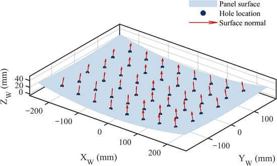
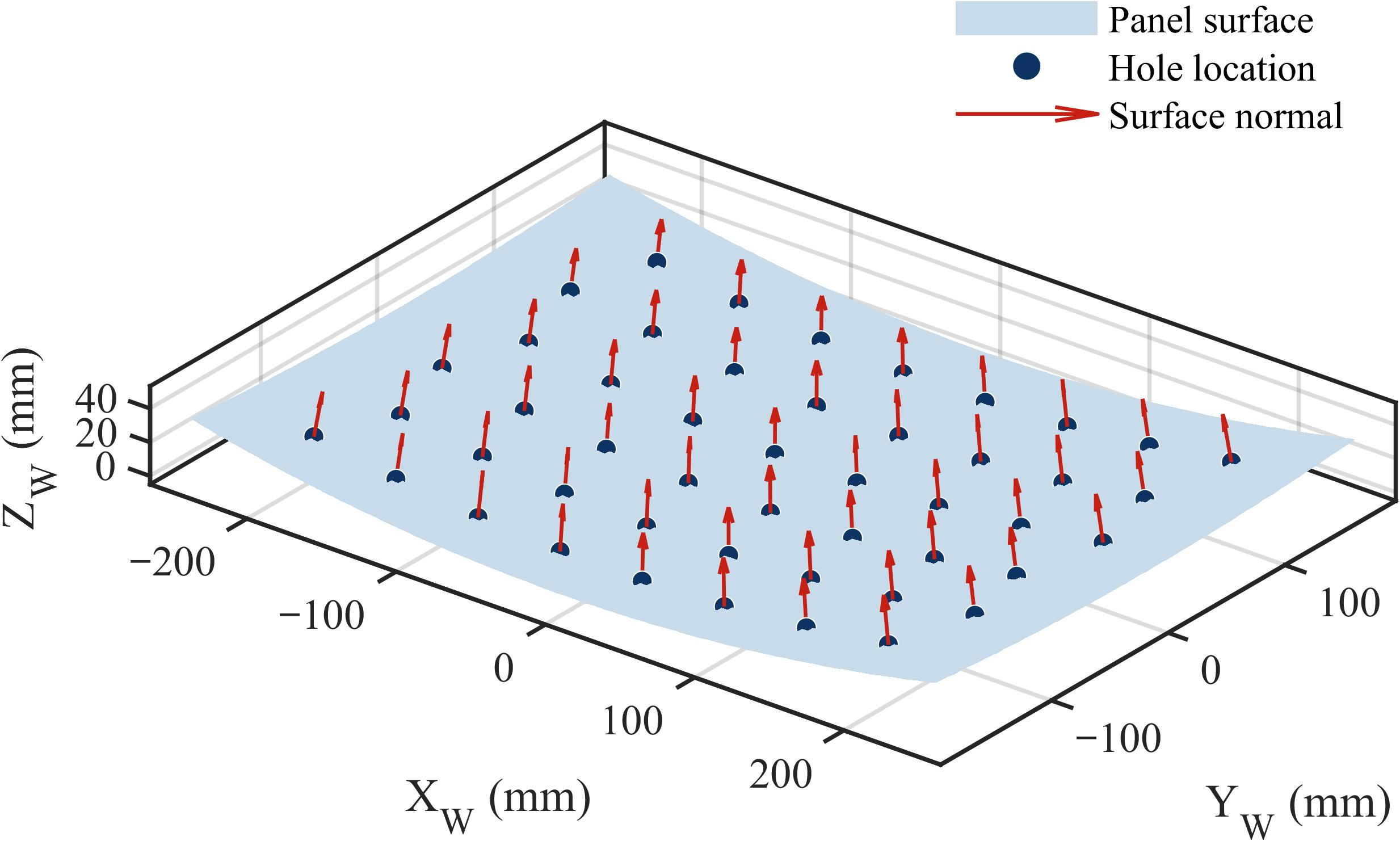
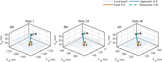
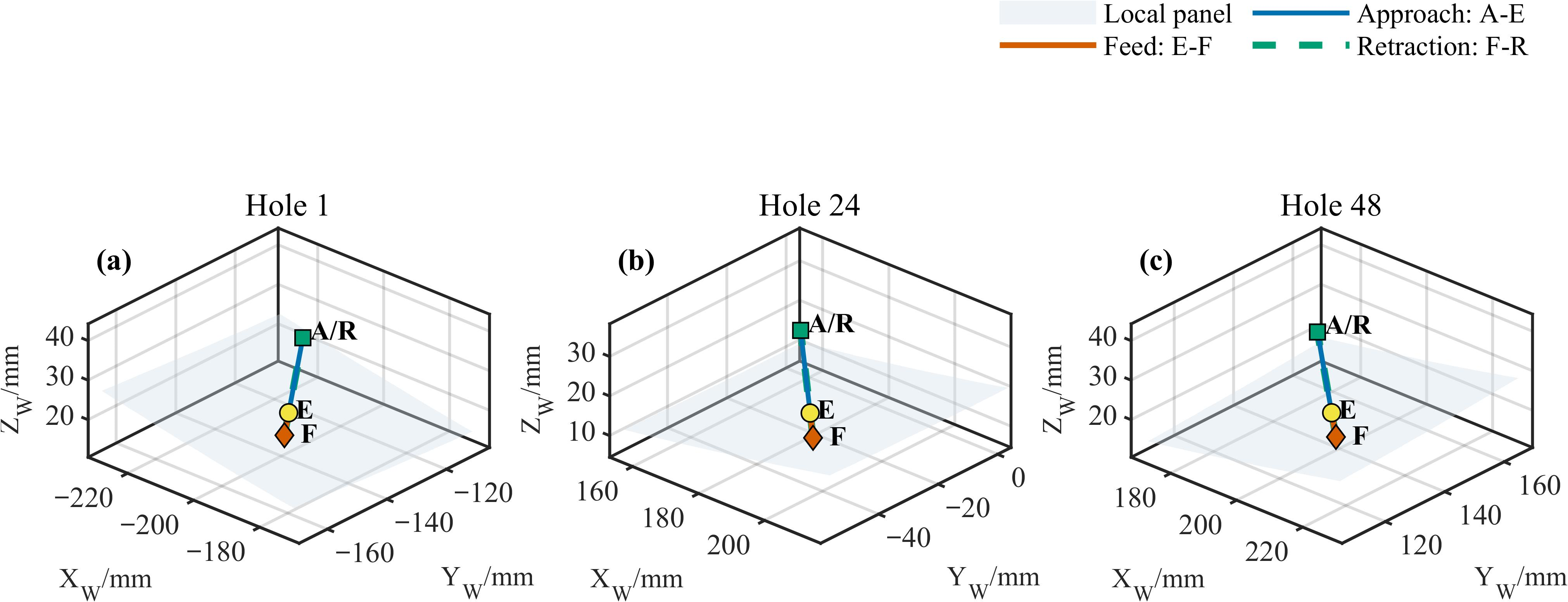
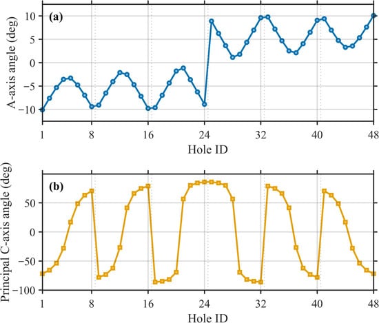
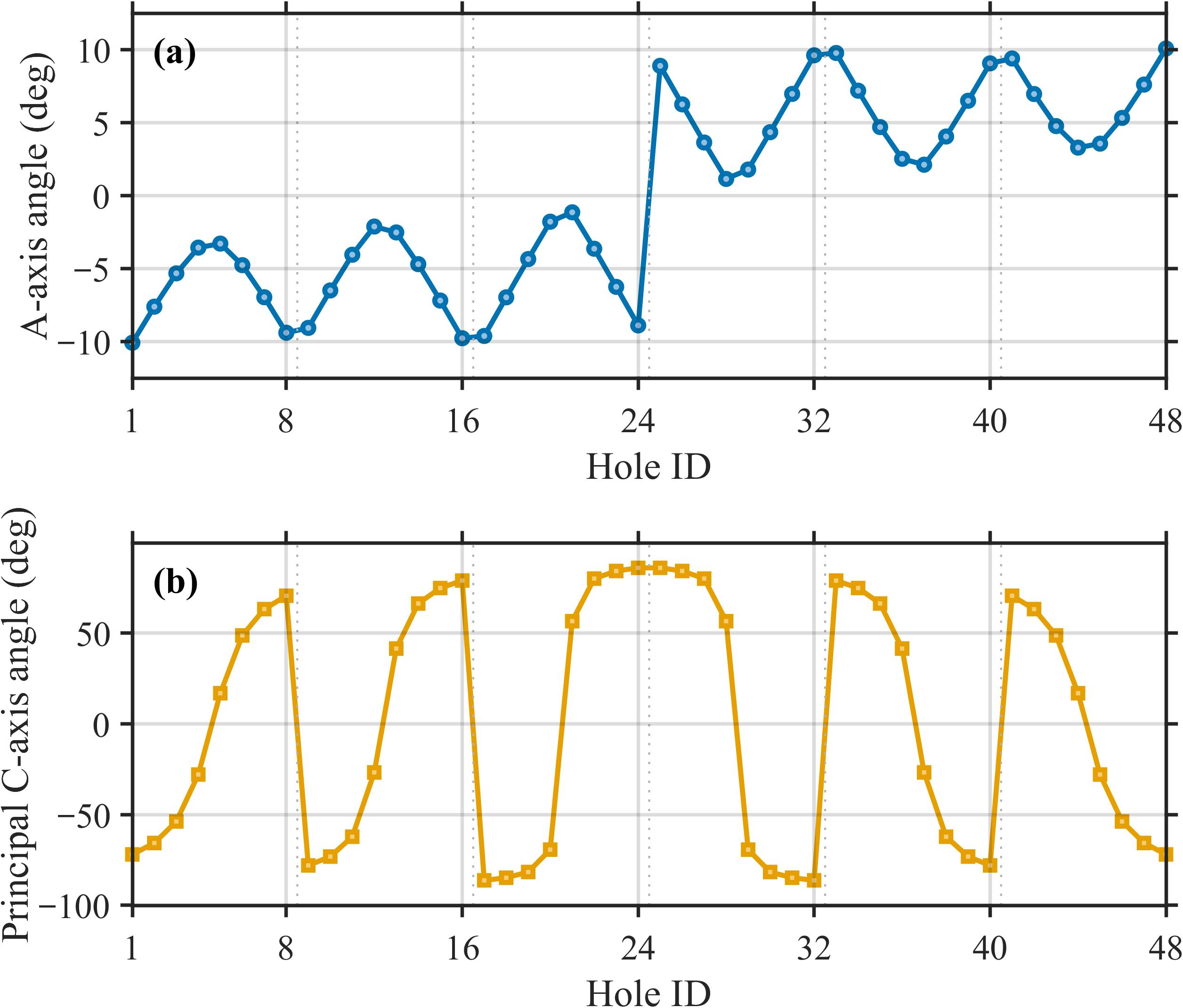
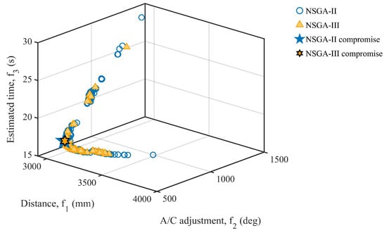
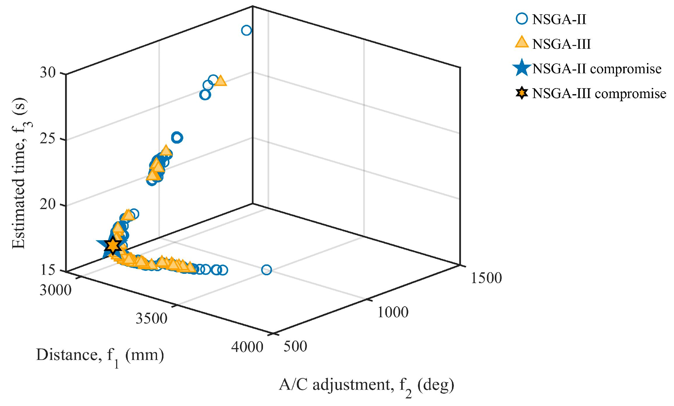
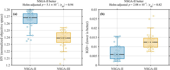
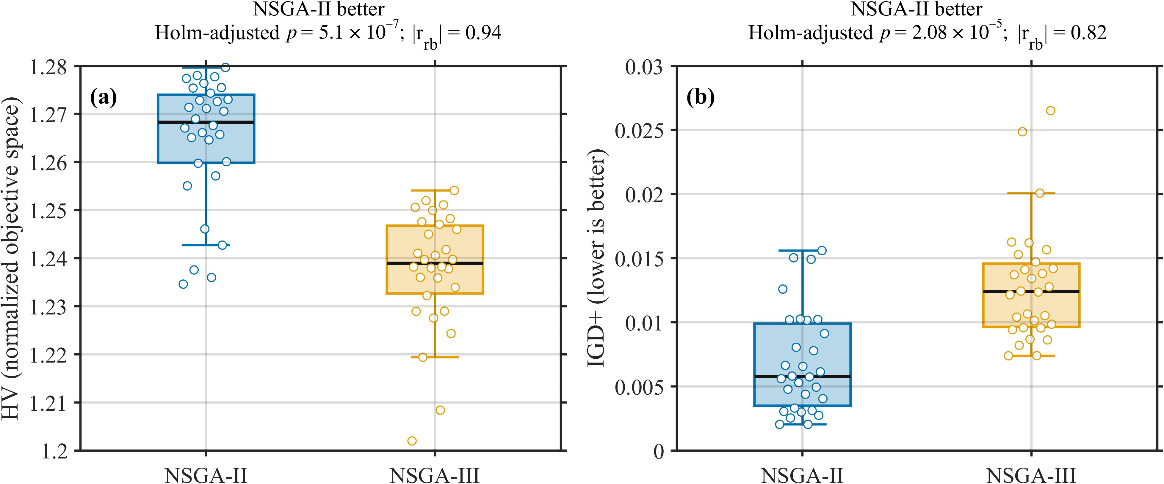
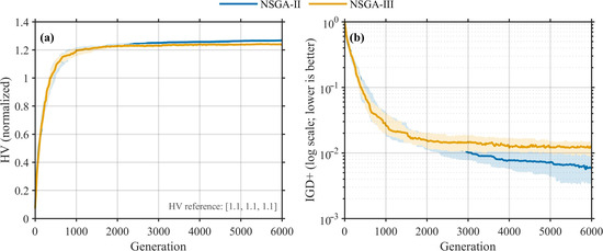
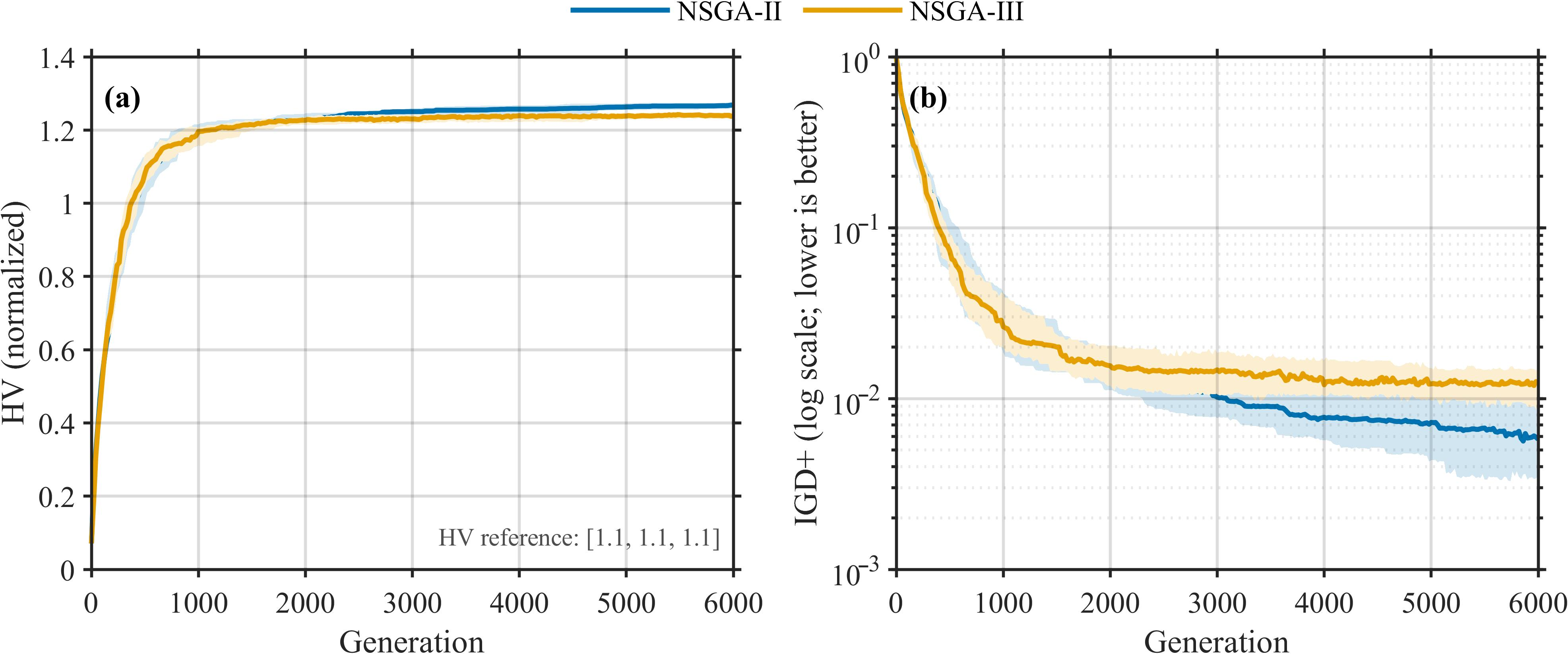
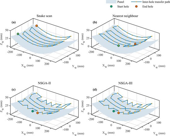
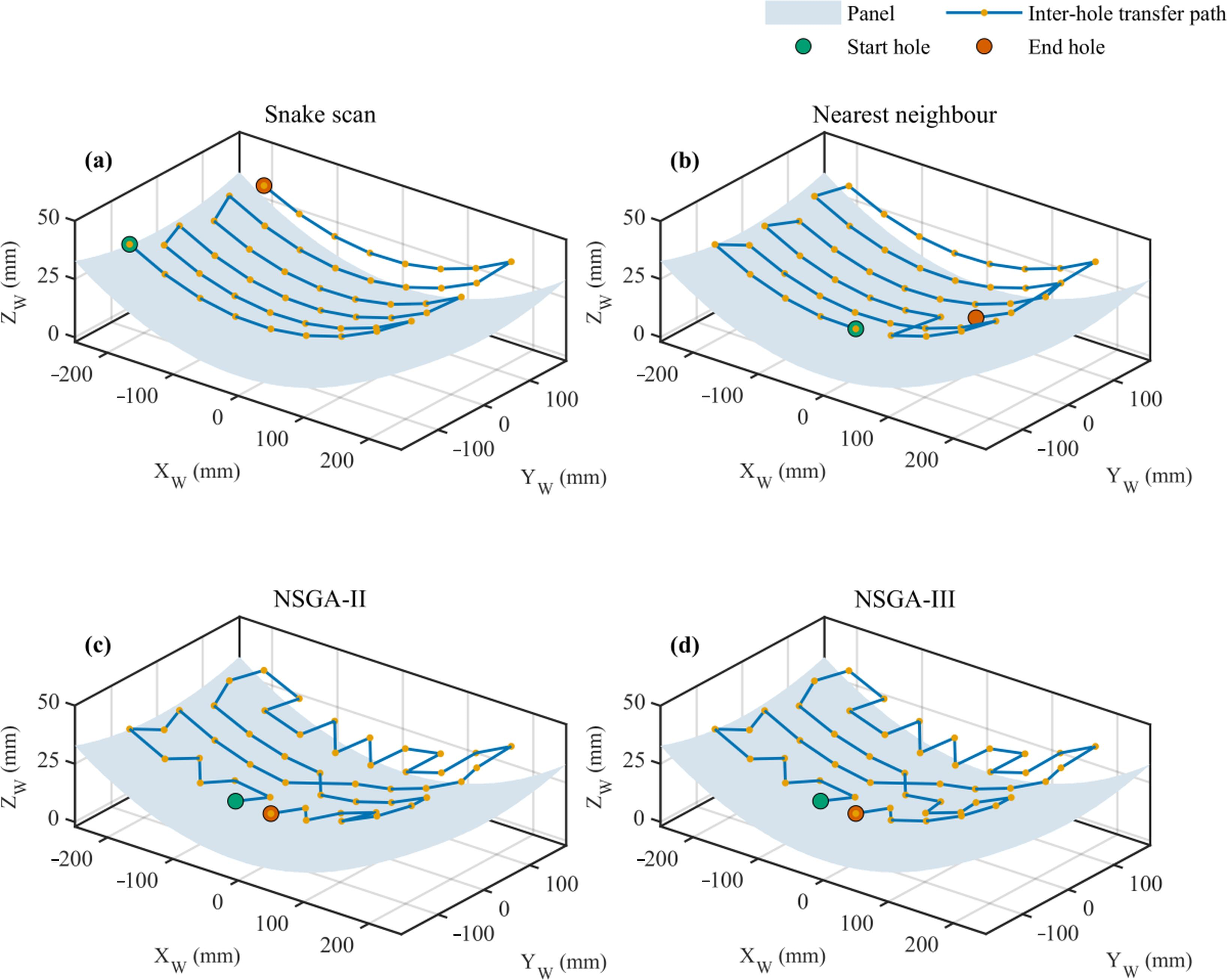
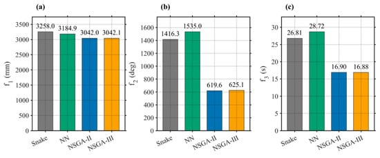
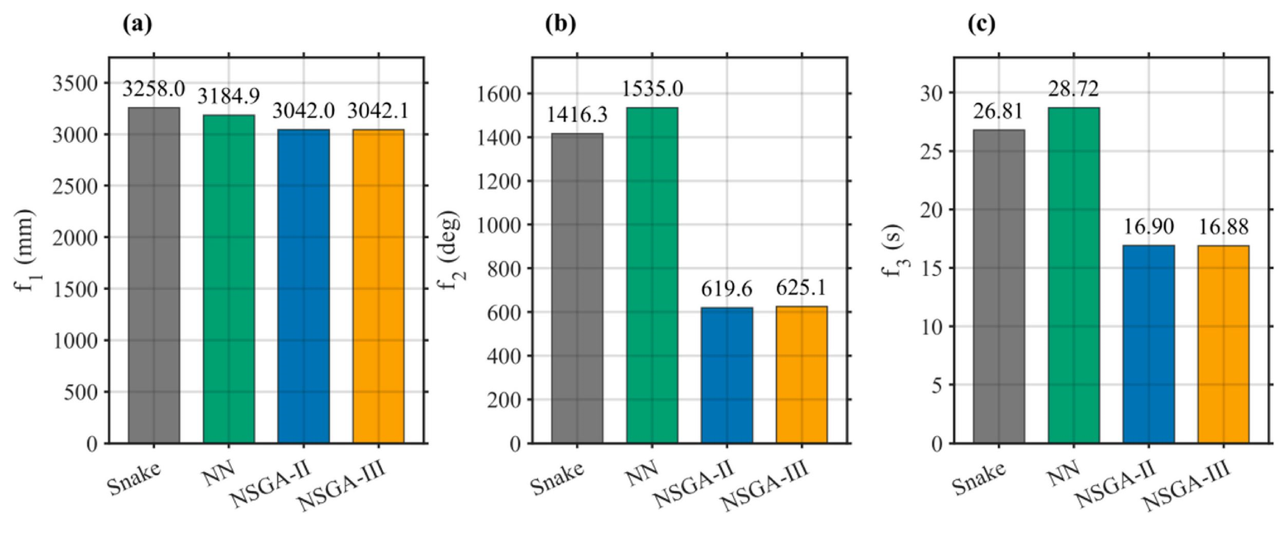
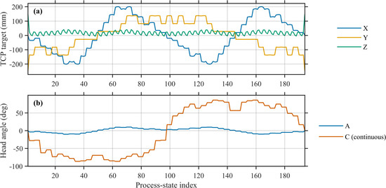
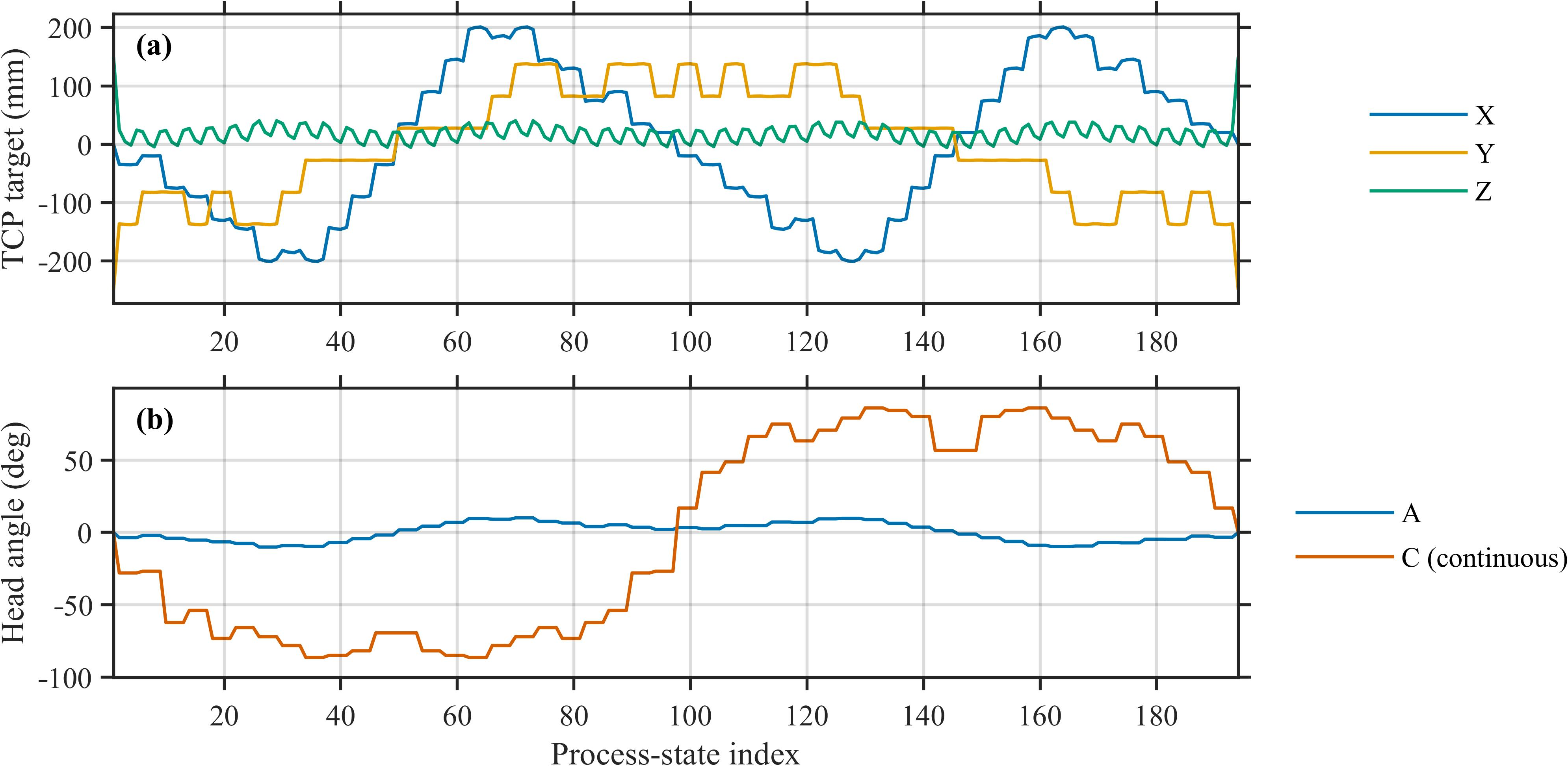
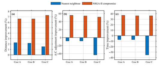
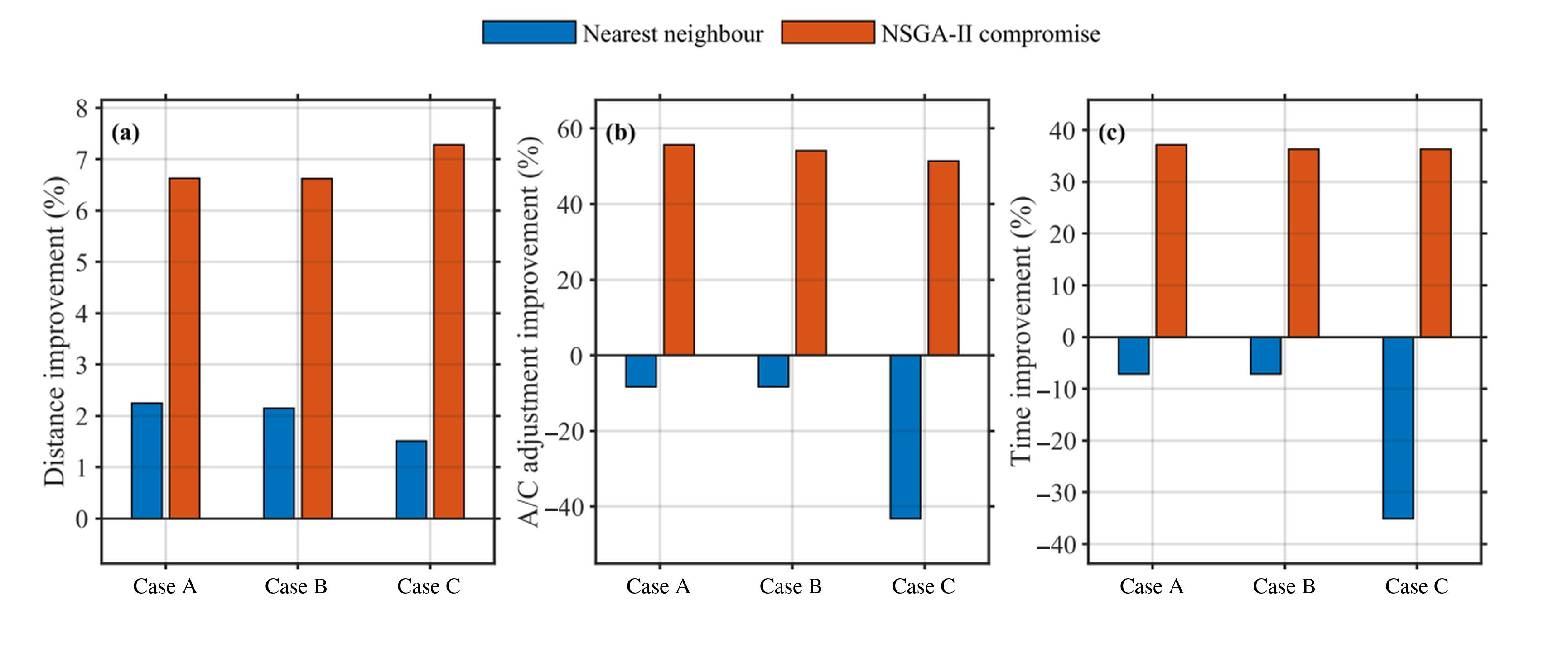
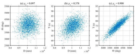
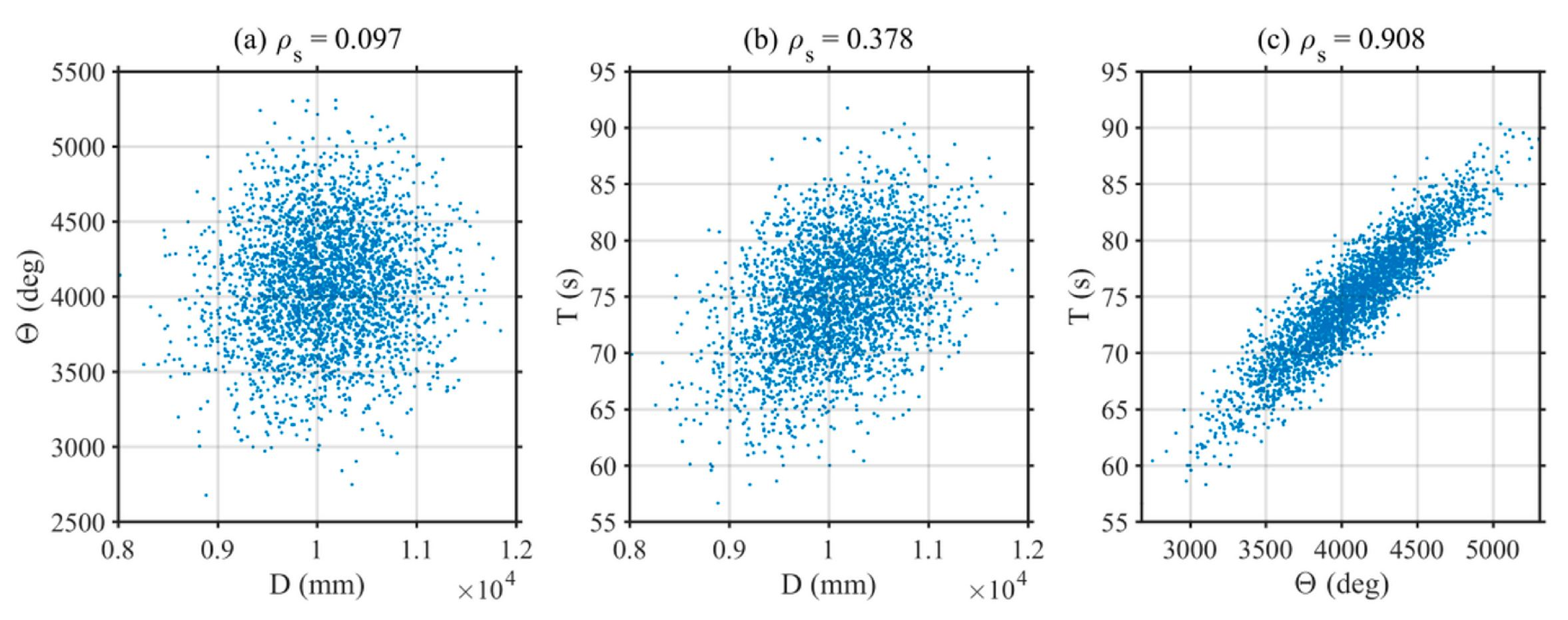
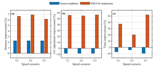
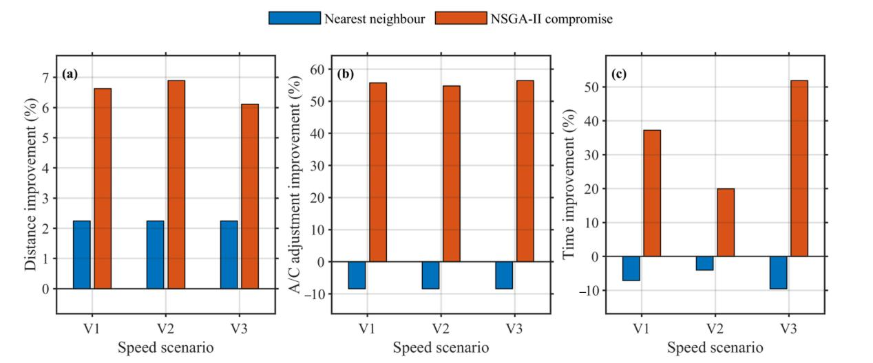

Disclaimer/Publisher’s Note: The statements, opinions and data contained in all publications are solely those of the individual author(s) and contributor(s) and not of MDPI and/or the editor(s). MDPI and/or the editor(s) disclaim responsibility for any injury to people or property resulting from any ideas, methods, instructions or products referred to in the content. |
© 2026 by the authors. Licensee MDPI, Basel, Switzerland. This article is an open access article distributed under the terms and conditions of the Creative Commons Attribution (CC BY) license.