Wave-Motion-Induced Photovoltaic Efficiency Correction for a Hybrid Wind–Solar Power Buoy in Offshore Cage Aquaculture: Modeling and Sensitivity Analysis

Abstract

Photovoltaic panels on a floating platform are tilted by wave-induced roll and pitch, and a tilted panel collects less light. This loss is usually neglected when hybrid wind–solar systems are sized. This paper estimates the loss for a small wind–solar buoy that powers offshore fish cages in the Yellow Sea. The buoy is modeled in ANSYS AQWA to obtain its roll and pitch response to waves, and the response is converted into a factor that corrects the calculated PV output. The factor depends on the square of the tilt amplitude and on the direct-beam fraction of the sunlight, so it can be evaluated directly once the wave response of the platform is known. Three buoy forms were compared, and a hemispherical buoy of 1.8 m diameter was selected. Its roll and heave natural periods, 2.86 s and 2.50 s, are shorter than the dominant wave period of 4.5–4.8 s, so the roll amplitude in the working sea state is only about 3° and the loss is only 0.1%. This is one to two orders of magnitude smaller than the 4–6% loss caused by the module temperature, so the static model is adequate for this buoy; the same factor gives 2–5% for a platform that rolls 15–25°, which shows when the wave motion has to be included in the energy balance. Wind speed and irradiance dominate the output, and a full-scale prototype confirmed the hydrodynamic and static power models to within 4%.

1. Introduction

1.1. Background and Motivation

Offshore cage aquaculture is growing fast in China, and a farm of the size considered here covers about 1.33 km² and holds more than 700 cages. It draws power all day for lighting, monitoring, feeding and data transmission, and a submarine cable is expensive to lay while a diesel generator has to be fueled and maintained. Renewable energy is the cleaner way to supply such a site [1,2,3], and a hybrid wind–solar system carried on a floating buoy is compact enough to serve one farm on its own [4]. The load is steady rather than peaky, which suits a renewable supply: the battery only has to cover the intervals when the wind and the sun are both weak.

Most sizing models for these systems treat the floating platform as if it were still. A real buoy is rolled and pitched by every wave, however, so the normal of the panel swings away from the sun many times a minute. The output of a module follows the cosine of the incidence angle, so the motion costs energy, and the size of the loss depends on the sea state rather than on the mounting angle alone [5,6,7]. The loss is small for a platform that barely moves and grows quickly once the motion becomes large, which is why it has to be quantified instead of assumed away. This paper quantifies the loss for a small hybrid buoy and links it to the design parameters. The result is a single multiplicative factor, so it can be added to an existing hybrid sizing model rather than only to the buoy studied here.

1.2. Related Work

Floating photovoltaic (FPV) systems have been studied from both the hydrodynamic and the electrical sides [8,9,10]. Wave-induced losses and wave-induced mismatch have been modeled for moored and articulated floating platforms [5,6], and experiments on floating arrays under regular and irregular waves have measured the loss directly and have shown how the layout of the array affects it [7,10]. Bifacial modules on a moving platform have been evaluated as well [8], and articulated arrays have been designed to adapt to the wave field instead of resisting it [9]. Much of this work concerns reservoirs and sheltered water, where a platform hardly moves, so the offshore case, where the waves are larger, is less well covered.

For offshore aquaculture, the power supply and the platform stability matter together [1,2,11]. Marine spatial planning studies show how a wave-powered farm can be sited and how its energy demand can be met from the sea [11], and techno-economic assessments of wave energy for aquaculture give the cost picture for comparable sites [2,4].

The hydrodynamic response of these platforms is well documented. Response amplitude operators have been computed for truss-type aquaculture platforms [12] and for small in situ buoys that have strict motion limits [13], and a floating semi-submersible that combines wind, solar and aquaculture has been tested experimentally [14]. Heave response operators for floating-collar membrane structures [15] and dynamic analyses of composite FPV structures that include wind–wave coherence and second-order wave loads [16] extend the same picture. These studies describe the motion of the platform; they stop short of the electrical output.

On the sizing side, several studies optimize the layout and the capacity of offshore hybrid wind–solar systems [17,18,19], and they show that the two resources complement each other over the day and over the season [20]. The gain they report comes from the resource and from the storage schedule; the motion of the platform is not part of the calculation.

Several recent studies address the same problem from the fluid-dynamic side. One surveys the problems that offshore floating photovoltaic structures face under wave and wind loads [21], and another evaluates the lifetime and power generation of such systems with wave motion and module degradation both included [22]. Two of them go a step closer to the electrical output: one computes the energy yield of an offshore floating array with the wave effects included [23], and the other couples the wave and wind loads to the light captured by a multi-body floating array [24]. These studies agree that the motion changes the output, and none of them reduces it to a correction that a sizing calculation can use.

Two problems remain: First, most hybrid-system models ignore the effect of buoy motion on PV efficiency. Second, no study ranks the main design parameters by their effect on the power output. This paper fills both gaps by proposing a motion-aware PV efficiency correction model and a sensitivity analysis.

1.3. Contributions

• A motion-aware PV efficiency correction method that links buoy roll and pitch to the PV incidence angle, giving a correction factor η_d that depends on the sea state.
• A comparison of three buoy shapes (cylindrical, truncated conical, hemispherical) that shows how to avoid resonance in the Yellow Sea.
• A sensitivity analysis that ranks wind speed, irradiance, battery capacity, and wave height by their effect on the power output.

1.4. Paper Organization

Section 2 describes the system, the buoy-form selection, and the stability check. Section 3 presents the hydrodynamic model and the PV efficiency correction model. Section 4 reports the sensitivity analysis. Section 5 reports the experiments. Section 6 discusses the results, and Section 7 concludes.

2. System Description and Buoy-Form Selection

2.1. Site and Design Basis

The site is the coastal water off Dalian in the northwestern Yellow Sea (38°43′–40°12′ N, 120°58′–123°31′ E). Local measurements and published data [7] give the design basis: an annual average wind speed of 6.0 m/s, a survival wind speed of 13.8 m/s (Force 6), a dominant wave period of 4.5–4.8 s, a working significant wave height of about 1.0 m, and a survival significant wave height of 6.5 m in typhoon conditions. These values set the turbine rating, the PV capacity, the draft and the survival requirements.

2.2. System Configuration and Power Demand

The aquaculture system covers about 2000 mu (≈1.33 km²) and contains two 50 m² floating monitoring platforms and more than 700 cages. The core loads are lighting, monitoring, feeding and data transmission (Table 1). Together they draw about 500 W continuously, so the daily energy demand, Equation (1), is:

E = P·t = 500 W × 24 h = 12 kWh

(1)

Table 1. Daily energy balance of the buoy at the design operating point. The four load categories of the design load schedule are listed with their rated power, duty cycle and daily energy. The rated powers are the design values used in Equation (1), and together they give the 500 W continuous demand, that is, 12.0 kWh/day. The generation is evaluated at the design operating point of 6 m/s wind and 800 W/m² irradiance, where the turbine and the array together deliver 500 W.

Item	Rated Power (W)	Duty Cycle	Energy (kWh/Day)
Lighting	150	continuous, 24 h/day	3.60
Monitoring: sensors, inclinometer, cameras	25	continuous, 24 h/day	0.60
Feeding actuators	300	continuous, 24 h/day	7.20
Data transmission	25	continuous, 24 h/day	0.60
Total demand, all loads	500	continuous, 24 h/day	12.0
Essential loads only (monitoring, communication, control)	33–50	continuous; 24–36 h autonomy	0.8–1.2
Generation at the design operating point
Vertical-axis wind turbine, 300 W rated	300	6 m/s reference, 24 h	7.2
PV array, 250 Wp total (two 125 Wp modules)	200	800 W/m2 reference, 24 h	4.8
Total generation at the design point	500	—	12.0
Storage
Lead–acid battery, 12 V/100 Ah	1.2 kWh nominal	—	—

To meet this demand the buoy carries a 300 W vertical-axis wind turbine (VAWT) and two 125 Wp monocrystalline PV modules, 250 Wp in total. Both feed a 12 V DC bus with a 12 V/100 Ah (1.2 kWh) lead–acid battery. A VAWT was chosen because it is compact and works in changing wind directions. The wind power and the PV power are estimated with Equations (2) and (3):

P_wind = ½·ρ_air·A·C_p·v³

(2)

P_pv = η_pv(T_c)·A_pv·G_POA, G_POA = G_b·cosθ + G_d·(1 + cosβ)/2 + ρ_g·G·(1 − cosβ)/2

(3)

where ρ_air is the air density, A the swept area, C_p the power coefficient, v the wind speed, A_pv the module area and θ the incidence angle. G_b = (1 − f_d)·G and G_d = f_d·G are the beam and diffuse components of the global irradiance G, f_d is the diffuse fraction, β is the module tilt measured from the horizontal, and ρ_g ≈ 0.06 is the sea-surface albedo [25]. The module efficiency depends on the cell temperature through η_pv(T_c) = η_ref·[1 + β_T·(T_c − 25)], with β_T the temperature coefficient of power; T_c is obtained in Section 3.4. At the representative operating point of 6 m/s wind and 800 W/m² irradiance, the turbine and the array deliver about 300 W and 200 W, a combined 500 W. The array rating is 250 Wp at standard test conditions, so the 200 W quoted here is its output at the 800 W/m² reference irradiance used throughout this study. The dynamic correction factor of Section 3.3 reduces the PV contribution by only about 0.1% for this stable buoy, so the corrected output is still about 500 W. The battery buffers the intermittent generation and carries the essential monitoring, communication and control loads (33–50 W) for 24–36 h without renewable input.

2.3. Buoy-Form Comparative Selection

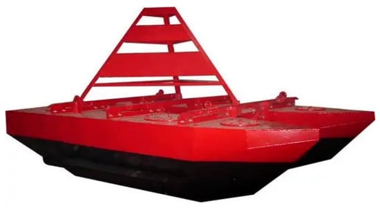
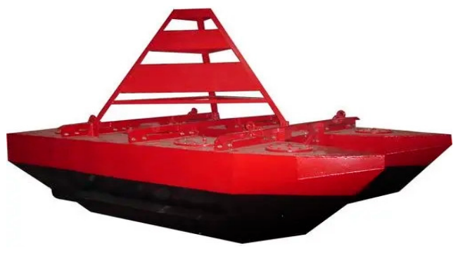
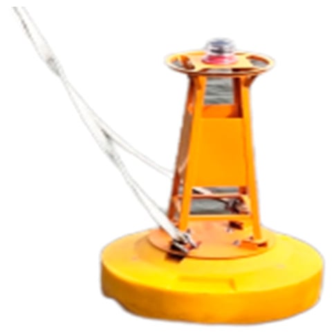
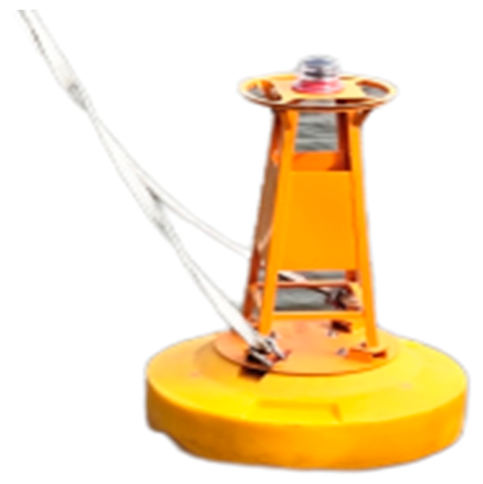
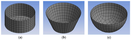
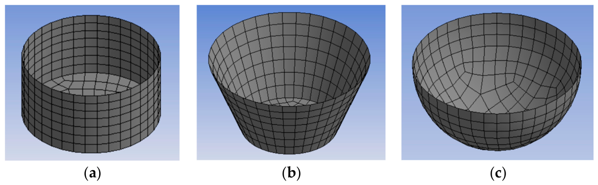
A disc-shaped buoy was chosen instead of a boat-shaped one because it follows the waves and is more stable (Figure 1). Figure 2 shows the common mode of the buoy. Three buoy forms were then compared at the same diameter (1.8 m) and the same depth (1.1 m): cylindrical, truncated conical and hemispherical (Figure 3). Their parameters are collected in Table 2.

Figure 1. Boat-shaped and disc-shaped buoy configurations.

Figure 2. Buoy common mode.

Figure 3. Geometry of the three candidate buoy forms: (a) cylindrical; (b) truncated conical; (c) hemispherical.

Table 2. Comparative parameters of the three buoy forms.

Parameter	Cylindrical	Truncated Conical	Hemispherical
Displacement volume (m3)	2.02	1.68	1.25
Roll peak period (s)	4.2	4.2	≈3.0
Heave RAO bandwidth (s)	2.8	2.4	1.5
Fabrication complexity	Low	Medium	Medium–high
Transportation efficiency	Low	Medium	High

The selection criterion was to keep the natural roll period as far as possible from the dominant wave band and the heave RAO bandwidth narrow. The cylindrical form displaces the most (2.02 m³) and so gives the greatest static buoyancy, but its roll peak period (4.2 s) sits inside the dominant wave period (4.5–4.8 s), which is a resonance risk. The truncated cone behaves in the same way. The hemispherical form has a roll peak period of about 3.0 s, well below the band, the narrowest heave RAO bandwidth (1.5 s), and a heave response that approaches unity at long periods, so it follows the waves closely. The detailed RAO analysis in Section 3.2 refines the hemispherical roll peak to 2.86 s. The hemispherical form was therefore selected despite its lower displacement, because motion stability and resonance avoidance matter more here. In the as-built buoy, the theoretical curvature was replaced by an inclined planar surface to simplify fabrication, and the molded depth was increased to carry the equipment. The basis of the comparison is as follows. The three forms were compared at equal principal dimensions—the same diameter (1.8 m) and the same molded depth (1.1 m)—rather than at equal displacement. Their masses, drafts, waterplane areas and hydrostatic stiffnesses are therefore not equal, so part of the difference between the computed natural periods comes from those quantities and not from the buoy form alone. Equal principal dimensions were chosen deliberately, because the constraints that bind here are the top area for the turbine and the modules, the fabrication envelope, and the transport and handling of the buoy. Under those constraints the comparison answers the design question that was actually posed. The comparison therefore ranks the three forms under the common envelope that this application imposes. At a common waterplane diameter the waterplane area and its second moment are nearly the same for the three forms, so the heave stiffness differs little between them and the natural periods separate mainly through the displaced volume, and hence through the draft and the metacentric height. A comparison at equal displacement, which would isolate the effect of buoy form itself, is a natural extension and is listed in Section 6 as future work.

2.4. Buoy Stability Verification

The buoy must not capsize under wind, current and wave loads, so its initial and large-angle stability were checked. The geometry, the draft and the limiting angles of the buoy follow the General Technical Specifications for Buoys (JT/T 760-2009 [26]), and the metacentric-height and stability-arm limits are taken from the Technical Regulations for the Statutory Survey of Sea-going Ships Engaged in Domestic Voyages (2020), issued by the Maritime Safety Administration of the People’s Republic of China, where those limits are specified. The vertical center of gravity Z_G and the center of buoyancy Z_B are referred to a coordinate system with its origin at the water surface on the buoy axis and positive upward. The buoy floats at a measured draft of 0.78 m. With a waterplane diameter of 1.8 m, the waterplane area is πD²/4 = 2.545 m², so the equilibrium displacement of the completed buoy is V = 2.545 × 0.78 = 1.985 m³, and its floating mass is M = ρV = 2034 kg. The center of gravity, taken from the SolidWorks assembly, is Z_G = −0.46 m, and the center of buoyancy is Z_B = −0.38 m. The displacement used in the stability check is therefore that of the complete floating assembly, which includes the ballast and the equipment carried on board. Table 2 reports a second volume for each candidate form: the enclosed volume at the common selection geometry, 1.25 m³ for the hemispherical form. The as-built body is fuller than that comparison form because its molded depth was increased and its curvature was replaced by an inclined planar surface (Section 2.3). The two volumes therefore describe two stages of the design, the bare form used for the selection and the completed buoy that was built. The nominal draft of 0.75 m quoted in Section 5.2 is the value that JT/T 760-2009 specifies for this class of buoy.

The initial (metacentric) stability is governed by the metacentric height GM = I/V + Z_B − Z_G, where I is the waterplane second moment of area and V the displaced volume. With I = πD⁴/64 = 0.5153 m⁴ for the 1.8 m waterplane, the metacentric height is GM = I/V + Z_B − Z_G = 0.260 + 0.08 = 0.34 m, which exceeds the 0.15 m minimum required by the standard and confirms adequate initial stability. The large-angle stability was then checked through the static stability arm; its maximum value was 0.32 m, exceeding the 0.20 m minimum required. Both checks confirm that the buoy meets the stability requirements.

3. Methodology: Hydrodynamic Modeling and Dynamic PV Efficiency Correction

3.1. Hydrodynamic Model

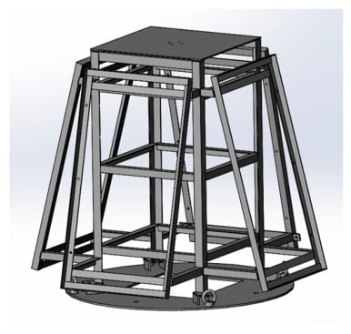
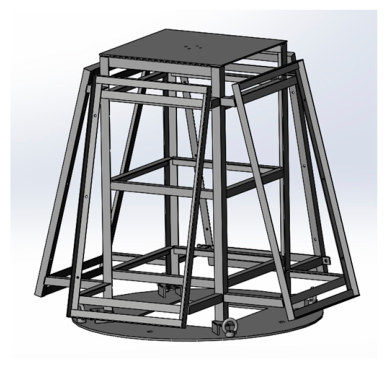
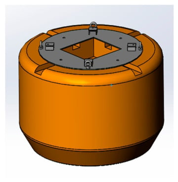
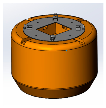
A hydrodynamic model of the buoy (1.8 m diameter, 0.78 m draft) was built in SolidWorks 2023 (Dassault Systèmes, Vélizy-Villacoublay, France) and imported into ANSYS AQWA 2023 R1 (ANSYS Inc., Canonsburg, PA, USA). The model links the buoy motion with the wind and solar power output. The total mass is 2034 kg, and the center of gravity comes from the SolidWorks assembly. The support frame and the watertight power compartment are shown in Figure 4 and Figure 5. A mesh study used three mesh densities (Table 3); the heave-RAO difference between the medium and fine meshes was 1.8%, so the medium mesh was used.

Figure 4. Support frame of the power equipment.

Figure 5. Watertight power compartment.

Table 3. Mesh-convergence study.

Mesh	Elements	Heave RAO Peak (m/m)	Relative Difference
Coarse	8432	1.15	4.5% vs. fine
Medium	16,894	1.12	1.8% vs. fine
Fine	33,786	1.10	reference

The marine environment was defined by a water depth of 40 m, a 50 m × 50 m domain, a seawater density of 1025 kg/m³, a gravity of 9.81 m/s², and a 200 s simulation with 0.05 s steps (4000 steps). Wind load was applied as a horizontal drag force from the basic wind-pressure formula, current load with the Morison equation, and wave load with the JONSWAP spectrum:

S(ω) = α·g²·ω⁻⁵ · exp[−(5/4)(ω/ω_p)⁻⁴] · γ^{exp[−(ω − ωp)2/(2σ2ωp2)]}

(4)

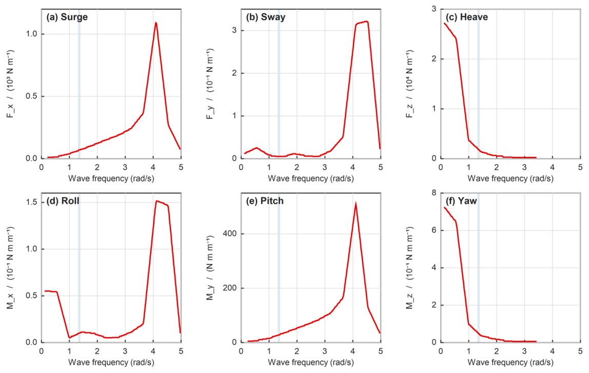
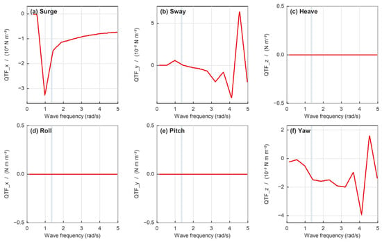
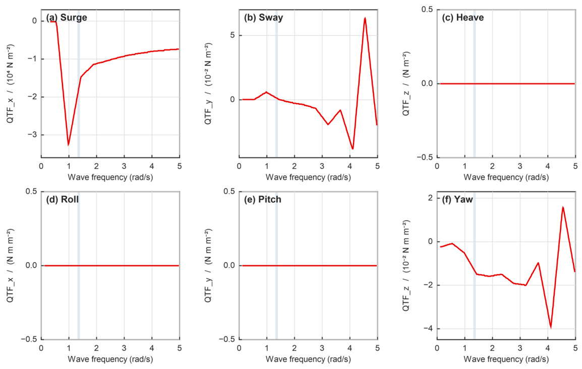
where α is the Phillips constant, γ = 3.3 is the peak-enhancement factor, σ = 0.07 for ω ≤ ω_p and σ = 0.09 for ω > ω_p, and ω_p is the peak frequency. First- and second-order wave forces were included. The first-order wave forces (diffraction and Froude–Krylov components) in the six degrees of freedom are shown in Figure 6a–f, and the second-order steady-drift forces in Figure 7a–f, which represent the slowly varying loads relevant to mooring-system design.

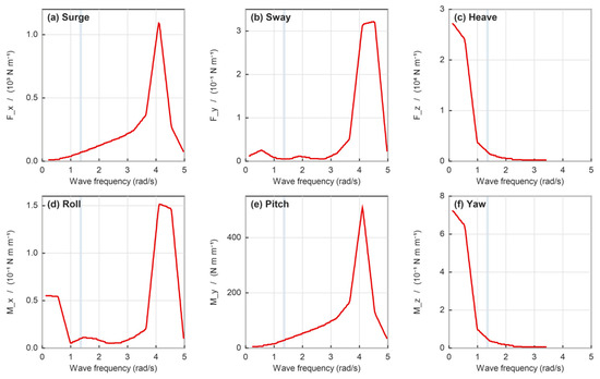
Figure 6. First-order wave excitation per unit wave amplitude for the hemispherical buoy at a 180° wave heading, computed in ANSYS AQWA from the diffraction and Froude–Krylov components of the JONSWAP spectrum (γ = 3.3) at 40 m water depth: (a) surge; (b) sway; (c) heave; (d) roll; (e) pitch; (f) yaw. The shaded band marks the dominant Yellow Sea wave period (T = 4.5–4.8 s, i.e., 1.31–1.40 rad/s). The excitation peaks at 4.0–4.2 rad/s (T ≈ 1.5 s); inside the dominant band the surge, sway and yaw forces remain a small fraction of their peak values, so the buoy is only weakly excited where it operates.

Figure 7. Second-order steady-drift excitation for the same buoy and heading, i.e., the slowly varying loads relevant to mooring design: (a) surge; (b) sway; (c) heave; (d) roll; (e) pitch; (f) yaw. Each panel has its own vertical scale because the components differ by orders of magnitude. The surge drift dominates, reaching −3.2 × 10⁴ N/m² near 1.0 rad/s; for this axisymmetric buoy at a 180° heading the heave, roll and pitch drift components are numerically negligible. The shaded band marks the dominant wave period (4.5–4.8 s).

Numerical Set-Up, Boundary Conditions and Mooring Assumption

The frequency-domain results reported below—the wave excitation and the response amplitude operators—were obtained with ANSYS AQWA-LINE, release 2023 R1, which solves the linearized, first-order, three-dimensional diffraction–radiation problem in the frequency domain by the boundary-element method. The velocity potential is decomposed into incident, diffracted and radiated components; the radiation and diffraction potentials are represented by a source distribution over the mean wetted surface of the body, and the free-surface boundary condition and the radiation condition at infinity are satisfied analytically by the Green function of the problem. The fluid domain is therefore treated as unbounded; no artificial far-field boundary or damping beach is required, and the panel mesh is applied to the wetted surface only. The panelization uses a mean panel edge length of approximately 0.016 m; the wetted-surface panel count is 16,894; and the total element count of the diffraction mesh is given in Table 3, together with the mesh-convergence study. The 50 m × 50 m region quoted above is the extent of the panelized region around the body and is not a wave tank with reflecting walls; in this formulation, the far field is handled analytically, so the size of that region does not introduce a spurious reflection. The 200 s run with 0.05 s steps mentioned above is the time-domain calculation of the buoy response in the JONSWAP sea state, driven by the hydrodynamic coefficients obtained from the frequency-domain solution.

The response amplitude operators and natural periods reported in Section 3.2 are those of the free-floating (unmoored) body. The mooring system is not represented in the hydrodynamic model. This was a deliberate restriction: the analysis was carried out to support the buoy-form selection and to establish the wave-frequency response, for which the unmoored body is the standard and conservative reference case, and the line properties of the as-built prototype were not available in a form that could be entered into the model.

For completeness we state how AQWA represents a mooring system, since a mooring contributes both stiffness and damping to the equations of motion. A mooring is modeled as a set of catenary or user-defined line elements attached to the body at specified fairlead positions. Each line is defined by its unstretched length, its mass per unit length in air and in water, its axial stiffness EA, and its hydrodynamic drag coefficient, and the solver accounts for seabed contact and friction. The resulting line tension is applied to the body as an external force. For a slack catenary mooring on a small buoy, the horizontal restoring force and the low-frequency damping act mainly on surge, sway and yaw, whereas the heave natural period is governed by the waterplane stiffness and the roll and pitch natural periods by the buoyancy-restoring moment, neither of which is materially changed by a slack chain.

The prototype test provides an empirical check on this reasoning. The buoy was tested while moored in a catenary configuration (Section 5.3.3), and its measured natural roll period, 2.82 s, agrees with the unmoored prediction of 2.86 s to within 1.4%. For this buoy and this mooring arrangement, the mooring therefore does not shift the wave-frequency natural period appreciably. A moored-versus-unmoored comparison that includes the line stiffness, damping and pretension is nevertheless desirable and is listed as an item of future work in Section 6.

Figure 6 and Figure 7 show the wave excitation in the six degrees of freedom for the hemispherical buoy at a 180° wave heading. For the first-order excitation, the response peaks between 4.0 and 4.2 rad/s (T ≈ 1.5 s), well above the dominant wave band; inside the shaded band, the surge, sway and yaw forces remain only a small fraction of their peak values, so the buoy is weakly excited where it actually operates. Heave and roll are the largest components. In the second-order steady-drift results, the surge component dominates, reaching −3.2 × 10⁴ N/m² near 1.0 rad/s, whereas the heave, roll and pitch drift components are numerically negligible for this axisymmetric buoy. No resonance appears in the main wave-frequency band, so the buoy is stable enough for long-term monitoring.

3.2. Motion Response and Resonance Avoidance

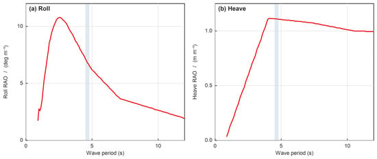
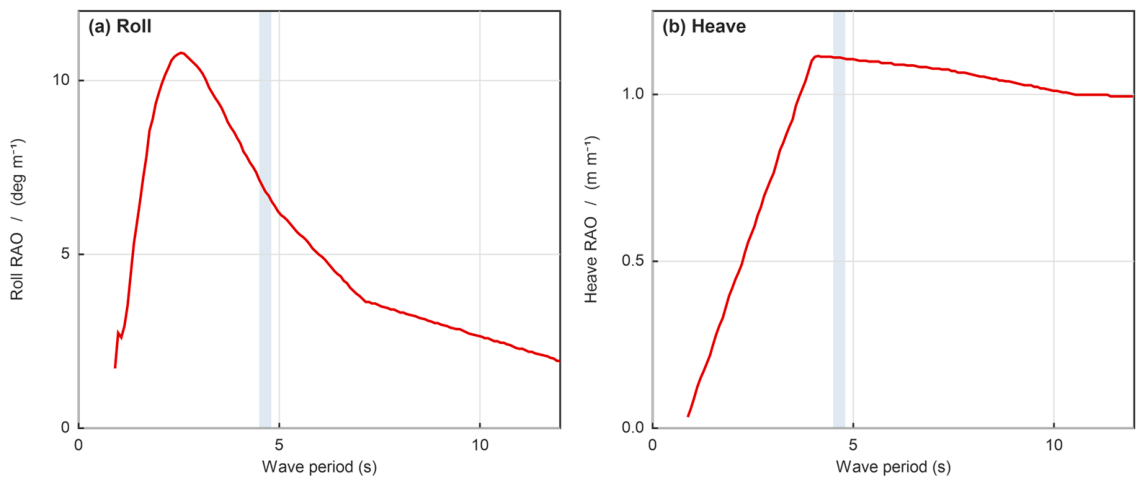
The roll RAO peaks at 10.8°/m at 0.35 Hz (period 2.86 s) (Figure 8a). The heave RAO rises to 1.12 m/m and stays close to unity at longer periods, so its maximum is broad rather than a sharp resonance (Figure 8b). In heave and roll, the buoy is only weakly excited, and no significant resonance coupling between roll and heave was observed. The radiation coefficients were also examined: the added mass peaked at 125.8 kg in sway and 58.8 kg·m² in roll, and a small resonance in the radiation (added-mass and damping) coefficients appeared near 4.1 rad/s, well outside the dominant wave-frequency range, further confirming resonance avoidance. Table 4 compares the natural periods with the dominant wave period band.

Figure 8. Response amplitude operators of the hemispherical buoy at a 90° wave heading, computed in ANSYS AQWA: (a) roll, which peaks at 10.8°/m at 0.35 Hz (T = 2.86 s); (b) heave, which rises to 1.12 m/m near the dominant wave period and stays close to unity at longer periods, so the heave response is wave-following rather than sharply resonant. The shaded band marks the dominant wave period (4.5–4.8 s). The roll maximum lies below that band, confirming resonance avoidance for the roll mode. The period axis is limited to 12 s, where the response has reached its asymptotic behavior.

Table 4. Natural periods relative to the dominant wave period.

Mode	Natural Period (s)	Dominant Wave Period (s)	Separation
Roll	2.86	4.5–4.8	36%
Heave	2.50	4.5–4.8	44%
Pitch	2.95	4.5–4.8	34%

All three natural periods (2.50–2.95 s) lie well below the dominant wave band (4.5–4.8 s), with separations of 34–44%, confirming resonance avoidance. The periods in Table 4 are obtained from the rigid-body mass matrix and the hydrostatic stiffness of the hydrodynamic model. For the heave mode the added mass is strongly frequency-dependent, so the RAO maximum is broad and lies at a longer period than this single-value estimate; the tabulated period is the design value used in the remainder of this paper.

The roll response maximum lies below the dominant band, and the heave response is wave-following rather than resonant, so the buoy does not resonate with the waves. The motion is small, so the sensors on board record the real operating state of the equipment rather than wave-induced noise.

The RAO maxima alone do not characterize the motion in an irregular sea, because the response is a narrow-band random process rather than a single amplitude. The response spectra S_r(ω) = |RAO(ω)|²·S_η(ω) were therefore evaluated with the JONSWAP spectrum of Equation (4) (γ = 3.3, T_p = 4.5 s) and the RAOs of Figure 8. The root-mean-square and significant amplitudes, and the expected value of the correction factor, are reported in Table 5. In the working sea state (H_s = 1.0 m), the roll angle has an RMS of 2.01° and a significant amplitude of 4.01°, and the heave motion has a significant amplitude of 0.51 m, that is, about half the significant wave height, which confirms the wave-following behavior inferred from Figure 8b. Because the problem is linear, the RMS and significant amplitudes scale in direct proportion to H_s at a fixed spectral shape.

Table 5. Response statistics in the JONSWAP design sea states, obtained from the response spectra S_r(ω) = |RAO(ω)|² S_η(ω). The significant amplitude is the mean of the highest one-third of the amplitudes. The expected correction factor is ⟨η_d⟩ = 1 − f_b(E[a_r²] + E[a_p²])/4 with E[a²] = 2m₀ for Rayleigh-distributed amplitudes and f_b = 0.8; the pitch amplitudes use the pitch/roll RAO ratio of 0.656 given in Section 3.3. In linear theory the amplitudes scale in proportion to H_s.

Sea State	Hs (m)	Tp (s)	RMS Roll (°)	Significant Roll (°)	Significant Pitch (°)	Significant Heave (m)	Expected ηd	Expected Loss (%)
Working	1.0	4.5	2.01	4.02	2.63	0.51	0.9993	0.07
Moderate	1.5	4.5	3.01	6.02	3.95	0.76	0.9984	0.16
Rough	2.0	4.5	4.01	8.02	5.27	1.02	0.9972	0.28
Extreme	6.5	4.5	13.05	26.10	17.12	3.30	0.9703	2.97

3.3. Dynamic PV Efficiency Correction Model

A model is developed here that corrects the PV power estimate for the effect of buoy motion. Two effects unrelated to motion dominate the instantaneous output, and both must be separated from it before the motion term can be interpreted: the split of the incident irradiance into beam and diffuse components and the module operating temperature. Both are therefore contained in Equation (3). When the buoy rolls and pitches, the panel normal rotates, so the instantaneous incidence angle θ(t) of direct sunlight deviates from its static design value. The instantaneous incidence angle is modeled as the static solar incidence angle plus the buoy-motion perturbation, Equation (5):

θ(t) = θ_s(t) + α_r·sin(ω_r·t) + α_p·sin(ω_p·t)

(5)

where θ_s(t) is the static incidence angle of the optimally tilted panel, α_r and α_p are the roll and pitch amplitudes in radians, and ω_r and ω_p are the roll and pitch frequencies in rad/s. All angular quantities in Equations (5)–(8) are in radians. The static incidence angle depends on the latitude φ, the solar declination δ, and the hour angle ω_h·t as in Equation (6):

cosθ_s(t) = sinδ·sin(φ − θ₀) + cosδ·cos(φ − θ₀)·cos(ω_h·t)

(6)

where θ₀ is the optimal static tilt angle. The dynamic efficiency correction factor η_d is defined as the ratio of the motion-averaged plane-of-array irradiance to its static value, Equation (7):

η_d = ⟨G_POA(t)⟩/G_POA,static

(7)

The roll and pitch amplitudes in Equation (5) are obtained from the RAO results of Section 3.2 for each sea state, so the model couples the hydrodynamic response to the electrical output. Because the wave period is much shorter than the diurnal variation of the sun, the static incidence angle and the static tilt are essentially constant over a wave cycle. Averaging over a cycle, the beam term of Equation (3) reproduces the quadratic reduction obtained previously, whereas the diffuse term, (1 + cosβ)/2, varies as −sinβ₀·δβ—an odd function of the motion whose cycle average vanishes. The diffuse component is therefore only second-order sensitive to the motion, and the closed-form correction becomes:

η_d ≈ 1 − f_b·(α_r² + α_p²)/4, f_b = G_b/G

(8)

where f_b is the beam fraction of the global irradiance and α_r and α_p are in radians—the cycle-averaged expansion that gives Equation (8) is a small-angle average and is valid only in radian measure. Including the diffuse component therefore makes the correction slightly smaller than a beam-only estimate, and it explains why η_d is intrinsically small for a compact, wave-following platform. For the clear-sky conditions assumed here, f_b ≈ 0.8; Table 6 gives η_d for both f_b = 1 (beam only) and f_b = 0.8, so that the sensitivity of the result to the assumed diffuse fraction is explicit.

Table 6. Dynamic efficiency correction factor versus sea state, for two values of the beam fraction of the global irradiance. The roll and pitch amplitudes are peak amplitudes for a regular wave of the stated height at the dominant period, obtained as RAO × H/2; they are not RMS values. The corresponding spectral statistics in an irregular sea are given in Table 5.

Wave Height (m)	Roll Amplitude (°)	Pitch Amplitude (°)	ηd (fb = 1)	ηd (fb = 0.8)	Loss
1.0 (working)	3.2	2.1	0.999	0.9991	0.09%
1.5	4.8	3.2	0.997	0.9980	0.20%
2.0	6.5	4.3	0.995	0.9963	0.37%
6.5 (extreme)	20.8	13.7	0.953	0.962	3.8%

Substituting the representative sea state (wave height 1.0 m, period 4.5 s) and taking f_b = 0.8, Equation (8) yields η_d ≈ 0.999, that is a ~0.1% reduction in PV efficiency. The two amplitudes are obtained by evaluating the roll and pitch RAOs in the dominant wave band (6.4°/m for roll and 4.2°/m for pitch) and multiplying by the wave amplitude of 0.5 m; this gives 3.2° and 2.1°, that is 0.056 rad and 0.037 rad. The correction is applied to the static PV output as in Equation (9):

P_pv,eff = η_d · P_pv,static

(9)

Table 6 summarizes the sea-state dependence of the correction factor. Because the loss scales quadratically with the motion amplitude, it stays below 5% for this compact, inherently stable buoy even in the extreme sea state. The same expression shows how quickly the loss grows once the platform motion becomes appreciable: with f_b = 0.8 and the pitch/roll ratio of 0.656, it gives 0.9% at 10° of roll, 1.9% at 15°, 3.5% at 20°, 5.4% at 25° and 7.8% at 30°. Equation (8) therefore applies beyond the wave-following regime as well, and these amplitudes define the design range used for that evaluation.

The model rests on two clearly stated assumptions: the panel is a rigid body whose orientation follows the buoy, and the beam efficiency follows the cosine of the incidence angle, with the angle-of-incidence modifier treated to first order. The diffuse component is included in Equation (3) through the standard view-factor relation for a tilted plane. Within these assumptions, the correction factor is multiplicative and sea-state dependent, so it should be propagated through the energy-yield estimate rather than treated as a constant. The model therefore plays a dual role: for the present compact, inherently stable buoy it indicates that the static model is adequate, while for larger, less stable platforms it provides the quantitative correction needed for credible energy-yield and sizing estimates.

3.4. Module Operating Temperature

Equation (3) makes the module temperature an explicit input, and its effect is much larger than the motion correction. Following the standard NOCT model, the cell temperature is T_c = T_a + (NOCT − 20)/800·G with NOCT = 45 °C, and the efficiency falls with temperature as η_pv(T_c) = η_ref·[1 + β_T·(T_c − 25)], where β_T ≈ −0.004 K⁻¹ for the monocrystalline modules used here [25].

At the representative operating point (G = 800 W/m², summer air temperature ≈ 24 °C), a land-based module would reach T_c ≈ 50 °C and lose about 10% of its rated efficiency. A floating module is in a different thermal environment: its back is coupled to the sea, which acts as a large heat sink. Even taking the summer sea-surface temperature (about 23 °C at the site) as the ambient temperature, the NOCT relation gives T_c ≈ 48 °C; reported floating photovoltaic installations, however, run several kelvin cooler than their land-based equivalents because of the additional heat path into the water [6,7]. Allowing an extra cooling of 8–13 K gives T_c between about 35 and 40 °C and a thermal loss of 4–6%. A nominal cell temperature of 40 °C is adopted in the remainder of this work, which corresponds to a 6% reduction in module efficiency; the lower bound of 35 °C would give 4%. The water cooling is therefore an advantage of floating PV, and it explains why the measured output in Section 5.4 lies close to the static prediction.

The relative magnitudes are as follows: a 10% change in irradiance changes the instantaneous PV output by about 9%, and the module temperature over its 35–40 °C range changes it by 4–6%, whereas the motion correction of Section 3.3 is about 0.1% at the operating sea state. The motion correction is therefore a design-model quantity whose magnitude, about 0.1%, is set by the sea state; Section 5.4 places it in the context of the prototype measurements.

4. Sensitivity Analysis and Design Implications

4.1. Method

We varied each parameter by ±20% from its baseline, keeping the others fixed, and computed the power output again at each point. The sensitivity index S_i is the percentage change in power output per percentage change in the parameter:

S_i = [P(+20%) − P(−20%)]/(0.4 · P_baseline)

(10)

Because the OAT method varies one parameter at a time and neglects interactions, the reported indices are first-order, local sensitivities; a global (e.g., Sobol) analysis and additional parameters (turbine rated power, panel tilt, battery depth of discharge) are left to future work.

4.2. Results

Figure 9 and Table 7 summarize the results.

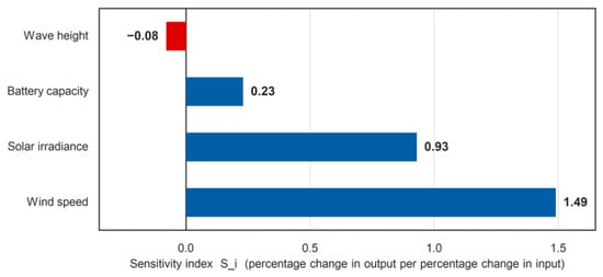
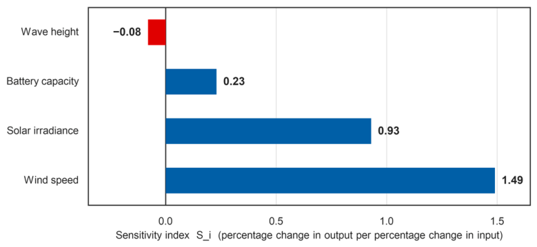
Figure 9. Sensitivity indices of the key parameters affecting the system power output, computed with Equation (10) from ±20% one-at-a-time variations of each parameter. Wave height is the only parameter with a negative index (−0.08), because a larger wave height increases the roll and pitch amplitudes and therefore reduces η_d through Equation (8).

Table 7. Sensitivity analysis results.

Parameter	Baseline	−20% Change	+20% Change	Sensitivity Index
Wind speed (m/s)	6.0	−28.3%	+31.2%	1.49
Solar irradiance (W/m2)	800	−18.5%	+18.5%	0.93
Battery capacity (Ah)	100	−4.5%	+4.5%	0.23
Wave height (m)	1.0	+1.2%	−2.1%	−0.08

4.3. Design Implications

Wind speed is the most sensitive parameter (index 1.49), followed by irradiance (0.93). So the turbine choice and the site wind data matter most. Battery capacity has a small effect (0.23) because it stores energy rather than generating it. Wave height has a small effect of the opposite sign (−0.08): a larger wave height increases the roll and pitch amplitudes, which reduces η_d through Equation (8) and hence reduces the PV output. It is the only negative index in Table 7, and it is consistent with the closed-form correction of Section 3.3. The design should therefore address the wind resource first and the PV sizing second. The motion correction is a small refinement of the PV output.

5. Experimental Validation

5.1. Prototype Fabrication

A full-scale prototype was fabricated with a high-strength polyethylene buoy and high-density rubber seals (commercially available marine-grade materials, China), a 300 W VAWT (Lanrunda, Dezhou, China), two 125 Wp monocrystalline PV modules (250 Wp total; Junda, Yangzhou, China), and a 12 V/100 Ah battery (Junda, Yangzhou, China). The buoy was thermoformed, and the chamber assembly used bolted connections with sealing compounds (commercially available, China).

5.2. Experimental Setup

The experiments were conducted at Bailanzi Fishing Port, Dalian, under real marine conditions, following the General Technical Specifications for Buoys (JT/T 760-2009): buoy diameter 1.8 m, nominal draft 0.75 m (minimum 0.70 m), maximum angling ≤ 15°, and the natural-roll-period band of 3–5 s specified for navigation buoys. The buoy-form selection of Section 2.3 deliberately seeks a shorter natural period, 2.86 s, so that the roll mode stays clear of the 4.5–4.8 s dominant wave band, and the prototype measurement of 2.82 s confirms that design target. Voltage was measured with a Fluke 287 multimeter (Fluke Corporation, Everett, WA, USA; ±0.025% + 5 digits), pressure with a digital manometer (Uni-Trend Technology, Dongguan, China; ±0.1% full scale), and inclination with a dual-axis inclinometer (Wuxi Beisensor Technology, Wuxi, China; ±0.1°); all instruments were calibrated before testing.

5.3. Experimental Results

5.3.1. Chamber Sealing

The power compartment was pressurized to 0.05 MPa, and the pressure was monitored for 10 min in three separate trials. The digital manometer used has an accuracy of ±0.1% of full scale, that is, ±0.05 kPa at the 50 kPa test pressure, and no trial showed a change in the indicated pressure larger than that resolution, so the compartment is pressure-tight to within the instrument. The largest leakage rate compatible with the observation, 0.05 kPa over a 50 kPa hold lasting 10 min, is 1.0 × 10⁻⁴ min⁻¹, or 0.01% of the gauge pressure per minute. The retention of the compartment is therefore bounded at a leakage rate of 1.0 × 10⁻⁴ min⁻¹. Table 8 lists this bound together with the test conditions and the resolution of the instrument on which it rests.

Table 8. Pressure-retention test of the power compartment. The change in the indicated pressure over the hold is smaller than the resolution of the manometer in all three trials, so the result is reported as the leakage bound that the resolution permits rather than as a decay record.

Quantity	Value
Test pressure	50 kPa (0.05 MPa)
Hold duration	10 min
Number of trials	3
Manometer accuracy	±0.1% of full scale = ±0.05 kPa at 50 kPa
Indicated pressure change over the hold	below ±0.05 kPa in all three trials
Largest leakage rate compatible with the observation	1.0 × 10−4 min−1 (0.01% of gauge pressure per minute)

5.3.2. Power Supply Stability

The output voltage was measured under 6 m/s wind and 800 W/m² irradiance (Table 9). The mean voltage was 12.47 V (SD 0.038 V, coefficient of variation 0.30%), within ±0.5% of the nominal 12.5 V, which demonstrates excellent voltage regulation. The 95% confidence interval of the mean is ±0.03 V (t(7) = 2.365), so the bus voltage is stable to within ±0.3% over the eight trials.

Table 9. Electrical operating point of the system at the design condition (6 m/s wind, 800 W/m²). The bus voltage, current, power and load resistance are listed for each of the eight trials, so that the repeatability of the operating point can be seen. The system supplies the 40 W essential load, the mid-point of the 33–50 W range, and the battery is on float, so the state of charge is 100%.

No.	1	2	3	4	5	6	7	8
Voltage	12.49	12.45	12.44	12.51	12.45	12.42	12.48	12.53
Current (A)	3.212	3.202	3.199	3.217	3.202	3.194	3.209	3.222
Power (W)	40.12	39.86	39.80	40.25	39.86	39.67	40.06	40.38
Load resistance (Ω)	3.89	3.89	3.89	3.89	3.89	3.89	3.89	3.89
Battery state of charge (%)	100	100	100	100	100	100	100	100

5.3.3. Structural Stability

The actual draft was 0.78 m (exceeding the 0.75 m nominal and 0.70 m minimum). The natural rolling period was measured at initial angles of 15°, 13°, 11°, 9°, and 7° at a 90° wave direction (Table 10). The period decreases with decreasing angle, consistent with the nonlinear restoring characteristics, and the maximum angular displacement remained below 15° in all trials. The 95% confidence intervals of the ten-trial means are ±0.03 s at 15°, ±0.05 s at 13°, ±0.05 s at 11°, ±0.03 s at 9° and ±0.06 s at 7° (t(9) = 2.262); the monotonic decrease in the period with decreasing initial angle is therefore well outside the measurement scatter.

Table 10. Rolling period (s) at 90° wave direction.

Angle	T1	T2	T3	T4	T5	T6	T7	T8	T9	T10	Mean	SD
15°	2.81	2.76	2.88	2.81	2.86	2.84	2.86	2.78	2.83	2.74	2.82	0.044
13°	2.47	2.39	2.58	2.55	2.49	2.39	2.51	2.44	2.41	2.45	2.47	0.063
11°	1.88	1.92	1.79	1.87	1.91	1.94	1.87	1.75	1.92	1.94	1.88	0.065
9°	1.59	1.49	1.61	1.58	1.51	1.56	1.61	1.62	1.58	1.57	1.57	0.042
7°	1.46	1.57	1.44	1.27	1.46	1.49	1.38	1.49	1.38	1.38	1.43	0.082

5.4. Simulation–Experiment Comparison

Table 11 compares the simulated and measured results; all relative errors are below 4%. The natural roll period (2.82 s measured vs. 2.86 s simulated, 1.4%) supports the hydrodynamic model on which the motion response, and therefore η_d, depends.

Table 11. Comparison of simulated and experimental results.

Parameter	Simulation	Experiment	Relative Error
Natural roll period (s)	2.86	2.82	1.4%
Buoy draft (m), nominal design	0.75	0.78 (as-built)	3.8%
Wind power at 6 m/s (W)	300	295	1.7%
PV output at 800 W/m2 (W)	200 (static)/≈200 (dynamic)	198	1.0% (static)

Table 12 gives the measurement uncertainty budget for this comparison. The combined standard uncertainty is 3.4%, dominated by the irradiance measurement, and the expanded uncertainty at 95% coverage (k = 2) is 6.7%. Both relative errors of Table 11 lie well inside this bound: 1.4% for the roll period and 1.0% for the PV output, where the measured 198 W is compared with the static prediction of 200 W at the reference condition of 800 W/m² irradiance and a 25 °C cell. The prototype therefore confirms the hydrodynamic model and the static PV and DC power models, and the same validated response operators give the motion correction of Equation (8). The module temperature enters the comparison through the budget of Table 12 (±1.5%) rather than as a separate correction. The expanded uncertainty of 6.7% also sets the resolution of the comparison, which is an order of magnitude above the 0.1% motion term; that term is therefore quantified from the validated hydrodynamic and spectral model, and the controlled motion-platform experiment described below measures it directly.

Table 12. Uncertainty budget for the PV-output comparison of Table 11.

Uncertainty Source	Standard Uncertainty	Basis
Plane-of-array irradiance (calibration, cosine response, spectral mismatch)	±3.0%	Instrument specification
Module temperature combined with β_T	±1.5%	±2 K; β_T = −0.4%/K
Voltage and current measurement (Fluke 287)	±0.03%	Instrument specification
Repeatability of the eight trials	±0.3%	Table 9 (coefficient of variation 0.30%)
Combined standard uncertainty (root-sum-square)	±3.4%	—
Effect to be resolved (ηd) at the working sea state	0.1%	Equation (8)
Ratio of resolution to effect	≈34	—
Expanded uncertainty U (k = 2, coverage ≈ 95%)	±6.7%	2 × uc
Ratio U/effect to be resolved	≈67	U/0.1%

Resolving a 0.1% PV loss in the field requires the plane-of-array irradiance to be known to better than 0.05%, which is beyond the accuracy of field pyranometers. A dedicated motion-platform experiment therefore provides the direct measurement: the module is mounted on a six-degree-of-freedom platform under a steady-state solar simulator with separately controlled beam and diffuse irradiance and compared with a stationary reference module of the same type. This is identified as the primary item of future work.

6. Discussion

The natural roll period of the hemispherical buoy (2.86 s) agrees with values reported for small floating PV platforms [6,8]. The correction factor shows that the motion-induced PV loss is about 0.1% for this stable buoy, so the static model is adequate here. The loss grows quadratically with the motion amplitude, however, and reaches 2–5% once the roll amplitude reaches 15–25°; this term has generally been neglected in hybrid-system sizing studies [17,18,19].

The sensitivity results show the same division of roles. Wind speed dominates the output, and the motion-induced PV loss (set by wave height through α_r and α_p) is a small correction on the PV share. So the design should first size the wind and PV parts, then add the motion correction and the battery check.

The scope of this study and the directions it opens are as follows: The three buoy forms were compared at equal principal dimensions, which ranks them under the common envelope set by the top area, the fabrication envelope and the transport limits of this application; a comparison at equal displacement isolates the effect of buoy form itself and is the natural next step. A seasonal campaign is under way to establish the long-term behavior, and the next campaign extends the structural tests to further wave headings. The correction factor η_d follows from the response operators that the roll-period comparison confirms to within 1.4%, and the controlled motion-platform experiment described above provides a direct measurement of it. The hydrodynamic model treats the free-floating body, and the measured roll period agrees with it to within 1.4%; a moored-versus-unmoored comparison that includes line stiffness, damping and pretension is the next step. The sensitivity analysis is one-at-a-time, and a global analysis will resolve the interaction effects. A techno-economic analysis will complete the design picture.

The buoy records its own inclination and motion together with the DC-bus voltage and the output power, without an external supply, and records of this kind are the input that fault-detection methods for photovoltaic arrays work from [27,28]. The platform therefore supplies both the power and the operating data that the condition monitoring of the equipment it carries needs.

7. Conclusions

This study designed, simulated, and tested a hybrid wind–solar buoy for offshore cage aquaculture. The main findings are as follows:

• A hemispherical buoy form was selected by comparative analysis, achieving natural periods (roll 2.86 s, heave 2.50 s) well separated from the dominant wave period (4.5–4.8 s) of the Yellow Sea and verified to meet the initial (GM = 0.34 m) and large-angle (static stability arm 0.32 m) stability requirements.
• A motion-aware PV efficiency correction methodology was developed that couples buoy roll and pitch to the instantaneous PV incidence angle through the response-amplitude operators, with the closed form η_d ≈ 1 − f_b(α_r² + α_p²)/4, where f_b is the beam fraction of the global irradiance; the loss is ≈0.1% for this stable buoy but scales quadratically with the motion amplitude, reaching 2–5% at roll amplitudes of 15–25°.
• A sensitivity analysis identified wind speed (index 1.49) and solar irradiance (0.93) as the dominant parameters, with battery capacity (0.23) and wave height (−0.08), the only negative index, of secondary importance to instantaneous output.
• The hydrodynamic and static power models were validated against a full-scale prototype: all relative errors are below 4%, and the natural roll period matches the simulation to within 1.4%, which confirms the response operators on which the motion correction rests.

Future work should include a controlled motion-platform experiment to measure η_d, a moored-versus-unmoored hydrodynamic comparison, motion-coupled PV tests, long-term field tests, and a techno-economic analysis. In summary, the buoy provides a reliable power platform for offshore aquaculture, the correction factor makes the sizing of such a system motion-aware, and the records the buoy makes of its own operation can support the condition monitoring of the equipment it carries.

References

- Manolache, A.I.; Andrei, G. A Comprehensive Review of Multi-Use Platforms for Renewable Energy and Aquaculture Integration. Energies 2024, 17, 4816. [Google Scholar] [CrossRef] [Scilit]
- Bertrand, M.; Giannini, G.; Majidi, A.G.; Senocq, C.; Rosa-Santos, P.; Clemente, D. Wave Energy Conversion to Decarbonize Offshore Aquaculture: Multi-Level Techno-Economic Analysis for a Case Study in Peniche, Portugal. Energies 2025, 18, 5934. [Google Scholar] [CrossRef] [Scilit]
- von Jouanne, A.; Agamloh, E.; Yokochi, A. A Review of Offshore Renewable Energy for Advancing the Clean Energy Transition. Energies 2025, 18, 4798. [Google Scholar] [CrossRef] [Scilit]
- Clemente, D.; Rosa-Santos, P.; Ferradosa, T.; Taveira-Pinto, F. Wave energy conversion energizing offshore aquaculture: Prospects along the Portuguese coastline. Renew. Energy 2023, 204, 347–358. [Google Scholar] [CrossRef] [Scilit]
- Nysted, V.S.; Stieng, L.E.S.; Kumar, M.; Roosloot, N.; Otnes, G.; Kjeldstad, T.; Selj, J. Modelling wave-induced losses for floating photovoltaics: Impact of design parameters and environmental conditions. Sol. Energy 2025, 293, 113439. [Google Scholar] [CrossRef] [Scilit]
- Polychronakis, K.; Korres, D.; Sammoutos, C.; Vidalis, E.; Tzivanidis, C. Frequency domain model of wave-induced mismatch in a moored floating solar platform with thermal effects. Sol. Energy 2026, 304, 114180. [Google Scholar] [CrossRef] [Scilit]
- Huang, L.; Yang, Y.; Khojasteh, D.; Ou, B.; Luo, Z. Floating solar power loss due to motions induced by ocean waves: An experimental study. Ocean Eng. 2024, 312, 118988. [Google Scholar] [CrossRef] [Scilit]
- Wijaya, O.; Ajmal, A.M.; Yang, Y. Performance Evaluation of Floating Bifacial PV Modules Considering Wave Motion. In Proceedings of the 2025 IEEE 3rd International Power Electronics and Application Symposium (PEAS); IEEE: Piscataway, NJ, USA, 2025; pp. 184–189. [Google Scholar] [CrossRef] [Scilit]
- Zhang, G.; Bao, F.; Jiang, C.; el Moctar, O.; Xu, Z.; Zhou, B. Hydrodynamic performance of floating solar arrays with articulated modules for optimal wave adaptation. Appl. Ocean Res. 2025, 164, 104762. [Google Scholar] [CrossRef] [Scilit]
- Yao, Y.; Li, M.; Yu, Z.; Qi, W.; Liu, Y.; Lian, J.; Yang, X.; Yang, X.; Liu, Z. Impact analysis of wave motion on power generation performance of offshore floating photovoltaic system. Sol. Energy 2026, 314, 114700. [Google Scholar] [CrossRef] [Scilit]
- Ewig, G.; Hasankhani, A.; Won, E.; Haji, M.N. Marine spatial planning techniques with a case study on wave-powered offshore aquaculture farms. Renew. Energy 2025, 238, 121791. [Google Scholar] [CrossRef] [Scilit]
- Cao, Y.; Li, Z.; Wang, K.; Ye, Q. Sensitivity of Dynamic Response of Truss-Type Aquaculture Platform to Floating Body Arrangement. J. Mar. Sci. Eng. 2024, 12, 431. [Google Scholar] [CrossRef] [Scilit]
- Cao, Y.; Wang, K.; Xi, C.; Wang, F. Hydrodynamic performance characteristics of small-scale in-situ buoys with critical motion requirements. Ocean Eng. 2024, 313, 119420. [Google Scholar] [CrossRef] [Scilit]
- Zhang, S.; Zheng, X.Y.; Liu, Y.; Jiang, Y.; Lei, Y.; Zhang, X.; Qian, K.; Li, X.; Shi, W. Nonlinear dynamic responses of a novel floating semi-submersible wind-solar-aquaculture hybrid system: An experimental study. Mar. Struct. 2025, 104, 103881. [Google Scholar] [CrossRef] [Scilit]
- Liu, H.; Han, Y.; Lian, J.; Liu, Y.; Yao, Y. Heave response amplitude operator of floating-collar membrane structures for FPV in regular waves. Ocean Eng. 2026, 343, 123173. [Google Scholar] [CrossRef] [Scilit]
- Xiao, Q.; Fang, H.; Song, Y.; Yan, Z. Dynamic response analysis of a composite offshore floating photovoltaic structure considering wind-wave coherence and second-order wave effects. Structures 2026, 88, 111939. [Google Scholar] [CrossRef] [Scilit]
- Kumar, S.; Panagant, N.; Arzaghi, E.; Baalisampang, T.; Garaniya, V.; Abbassi, R. A multi-objective optimisation framework for a standalone hybrid offshore renewable energy system with electrical and hydrogen loads. Energy 2025, 330, 136826. [Google Scholar] [CrossRef] [Scilit]
- Pei, A.; Qi, X.; Yang, Z.; Li, T.; Xu, X.; Wang, Y. Coordinated Optimization of Wind-Photovoltaic-Hybrid Energy Storage System in Offshore Isolated Power Grids Considering Wind-Photovoltaic Complementary and Frequency Stability. In Proceedings of the 2025 28th International Conference on Electrical Machines and Systems (ICEMS); IEEE: Piscataway, NJ, USA, 2025; pp. 3305–3310. [Google Scholar] [CrossRef] [Scilit]
- Rehman, S.; Menesy, A.S.; Zayed, M.E.; Zaery, M.; Al-Shaikhi, A.; Mohandes, M.A.; Irshad, K.; Kassas, M.; Abido, M.A. Synergistic sizing and energy management strategy of combined offshore wind with solar floating PV system for green hydrogen and electricity co-production using multi-objective dung beetle optimization. Results Eng. 2025, 25, 104399. [Google Scholar] [CrossRef] [Scilit]
- Shao, M.; Han, Y.; Sun, J.; Xu, H.; Kong, X.; Wang, H.; Wang, B.; Shao, Z.; Guan, J.; Qu, Z. Bi-level multi-objective optimization of configuration and scheduling of offshore wind-solar-storage hybrid power system considering demand response. Ocean Eng. 2026, 352, 124614. [Google Scholar] [CrossRef] [Scilit]
- Jin, R.; Geng, B.; Zhao, X.; He, M. An overview for offshore floating photovoltaic structures and their fluid dynamic issues. Phys. Fluids 2025, 37, 061301. [Google Scholar] [CrossRef] [Scilit]
- Jin, H.; Kong, X.; Wang, C.; Liu, H.; Yao, Y. Lifetime and power generation evaluation of offshore floating photovoltaic systems considering wave motion and photovoltaic module degradation rates. J. Clean. Prod. 2025, 526, 146659. [Google Scholar] [CrossRef] [Scilit]
- Fu, J.; Zhao, Y.-P.; Jia, G.-C.; Ma, C.; Shu, J.-Q.; Sun, Y.-Q. Numerical study on wave–wind coupling effects on hydrodynamics and light capture performance of offshore multi-body floating photovoltaic system. Ocean Eng. 2025, 323, 120593. [Google Scholar] [CrossRef] [Scilit]
- Alcañiz, A.; Monaco, N.; Isabella, O.; Ziar, H. Offshore floating PV–DC and AC yield analysis considering wave effects. Energy Convers. Manag. 2024, 300, 117897. [Google Scholar] [CrossRef] [Scilit]
- Duffie, J.A.; Beckman, W.A. Solar Engineering of Thermal Processes, 4th ed.; John Wiley & Sons: Hoboken, NJ, USA, 2013; ISBN 978-0-470-87366-3. [Google Scholar]
- JT/T 760-2009; Navigation Mark Layout Requirements for Inland Waterways. Ministry of Transport of the People’s Republic of China: Beijing, China, 2009.
- Liu, Y.; Chen, L.; Zhu, Y.; Li, K.; Cai, D.; Xiong, L.; Shi, H. Intelligent photovoltaic array fault diagnosis via RIME optimized hybrid deep learning model. Sol. Energy 2026, 315, 114826. [Google Scholar] [CrossRef] [Scilit]
- El-Banby, G.M.; Moawad, N.M.; Abouzalm, B.A.; Abouzaid, W.F.; Ramadan, E.A. Photovoltaic system fault detection techniques: A review. Neural Comput. Appl. 2023, 35, 24829–24842. [Google Scholar] [CrossRef] [Scilit]
Disclaimer/Publisher’s Note: The statements, opinions and data contained in all publications are solely those of the individual author(s) and contributor(s) and not of MDPI and/or the editor(s). MDPI and/or the editor(s) disclaim responsibility for any injury to people or property resulting from any ideas, methods, instructions or products referred to in the content. |
© 2026 by the authors. Licensee MDPI, Basel, Switzerland. This article is an open access article distributed under the terms and conditions of the Creative Commons Attribution (CC BY) license.