


Abstract
This study investigates predictive maintenance for SCADA-controlled pump stations using multi-sensor data processing and hybrid machine-learning models. The conventional maintenance approaches adopted in practice remain reactive, with little provision for actual early warnings under real-world conditions such as noisy data, class imbalance, or varying sensor dynamics. A data-driven solution is proposed to predict pump tripping events using operational SCADA system data for early warning with useful lead times. The dataset, obtained from a water-utility SCADA system, contained missing values, heavy-tailed sensor distributions, and substantial class imbalance. The preprocessing strategy used time-aware imputation, winsorisation, and a sliding-window configuration informed by the characteristics of the SCADA data. Benchmark machine-learning models achieved PR-AUC values of approximately 0.55 or lower for trip-escalation prediction, highlighting the difficulty of predicting rare trip events directly from SCADA data. The proposed hierarchical GRU-based framework achieved PR-AUC values exceeding 0.80, demonstrating a substantial improvement in predictive performance while maintaining high precision and low false-alarm rates. In addition, a Remaining Useful Life (RUL) component was included to extend the system to support near-term risk forecasting. Even so, long-term forecasts remained uncertain, indicating that further model development is required.
1. Introduction
Urban water distribution systems depend on the reliable operation of pump stations to maintain adequate flow and pressure across domestic, industrial, and municipal networks [1,2]. These stations include electromechanical subsystems, such as pumps, motors, instrumentation, and control systems, that are critical to ensuring service continuity. In both developed and developing regions, these systems face growing operational pressure due to ageing infrastructure, demand growth, and maintenance inefficiencies [3]. In rapidly urbanising areas like Gauteng, South Africa, water utilities are especially strained as they work to meet the national service delivery targets outlined by the Department of Water and Sanitation (DWS) [4]. Despite their importance, pump stations are often maintained using conventional strategies such as reactive maintenance (RM), where intervention occurs only after failure, or time-based preventive maintenance (PM), where servicing is scheduled without regard to actual equipment condition [5,6]. These approaches are increasingly viewed as inefficient, as they offer limited protection against sudden breakdowns and can lead to premature maintenance actions that reduce asset life [7,8]. Globally, poor maintenance strategies are estimated to cost industries over USD 222 billion annually, with reactive practices representing a significant share [9]. In the South African context, these limitations are not theoretical. Recent pump station failures have led to severe regional water shortages, as seen in the 2024 outage at a key Gauteng booster station, where a 68% drop in pumping capacity disrupted supply to Ekurhuleni and Tshwane [10]. Similarly, failures at the Bronkhorstspruit Water Treatment Plant in the same year led to weeks-long supply disruptions due to delayed spare part procurement [11]. These incidents underscore the need for more advanced maintenance strategies that can anticipate faults and prevent cascading failures.
Predictive maintenance (PdM), which aligns with the principles of Reliability-Centred Maintenance (RCM), has emerged as a data-driven alternative to RM and PM. PdM relies on real-time or historical condition monitoring data to predict equipment failures and optimise maintenance planning [12,13]. Supported by advances in artificial intelligence (AI) and machine learning (ML), PdM enables utilities to reduce unplanned downtime, extend equipment life, and improve asset reliability. Studies across sectors have shown PdM reducing downtime, increasing uptime, and lowering operational costs [14,15]. Supervisory Control and Data Acquisition (SCADA) systems play a central role in PdM implementation. Widely adopted in water utilities, SCADA systems provide real-time visibility of key parameters, including flow, pressure, vibration, and pump status [16,17]. These systems are designed for control and monitoring, using Programmable Logic Controllers (PLCs), Human-Machine Interfaces (HMIs), and historical data repositories [18]. However, SCADA platforms typically operate reactively, whereby alarms are triggered only when thresholds are breached, limiting their usefulness for fault prediction. While these systems collect high-frequency time-series data, much of it is underutilised due to noise, incomplete annotations, irregular sampling, and class imbalance [19,20]. Machine learning models have emerged as powerful tools for extracting predictive insights from industrial time-series data. Supervised models, such as Random Forests (RF), Support Vector Machines (SVM), and XGBoost, have been widely used in fault classification and anomaly detection [21,22]. Deep learning methods, including Long Short-Term Memory (LSTM) and Gated Recurrent Units (GRU), are particularly well-suited to modelling time-dependent degradation patterns [23]. Hybrid approaches that combine temporal learning with ensemble methods have outperformed stand-alone models in several infrastructure monitoring applications [24].
Nonetheless, applying machine learning to SCADA system data presents unique challenges. These include class imbalance, missing data, limited fault labels, and fragmented SCADA system architectures [25,26,27]. Addressing these issues requires robust preprocessing, including time-aware imputation, smoothing, noise reduction, and windowing techniques [28]. Class-imbalance mitigation strategies such as the Synthetic Minority Oversampling Technique (SMOTE), hybrid sampling, and cost-sensitive learning have also shown promise [29]. For deployment in operational environments, model interpretability techniques such as SHapley Additive exPlanations (SHAP) and Local Interpretable Model-Agnostic Explanations (LIME) are essential for building stakeholder trust [30]. While international utilities in the United States, Europe, and Asia have demonstrated the benefits of PdM in water infrastructure (e.g., PIPEiD, MPWiK, and HxGN EAM) [31,32,33], South African water utilities have not followed suit. Instead, PdM adoption has been more prominent in adjacent sectors such as power and mining, where digital maturity and financial capacity are generally higher. In the water sector, SCADA systems are often siloed, underutilised, and disconnected from maintenance planning processes. Few studies have focused on integrating historical SCADA data with machine learning to develop predictive maintenance capabilities for South African pump stations.
Existing research relevant to this study can be divided into three main strands. Water-infrastructure studies have largely examined network-level problems such as pipe failure, leakage, deterioration, and rehabilitation planning [26,27]. Pump-focused research has concentrated mainly on condition monitoring, fault diagnosis, and the classification of known mechanical or electrical faults using signal-processing and machine-learning methods [34,35]. More recent studies have used operational pump data for unsupervised anomaly detection and explainable field diagnosis, showing the value of multivariate feature extraction, maintenance records, and deployment-oriented analysis [36,37]. These strands provide useful methods for asset monitoring, but anomaly detection, fault classification, trip-escalation prediction, and prognostic estimation are generally considered as separate tasks.
The application of these methods to operational water-pump SCADA data remains difficult. Fault observations are limited, class distributions are highly imbalanced, sensor quality is inconsistent, and operational interventions can obscure the progression of degradation. In addition, detecting abnormal behaviour does not establish whether the condition will develop into a protective trip or provide an estimate of the remaining intervention time. This creates a need for a staged framework that links temporal anomaly detection with fault-conditioned escalation prediction and short-horizon maintenance support using the data already available in the SCADA historian.
This study develops and evaluates a predictive maintenance framework for a large-scale bulk-water pumping station using historical SCADA data. The framework combines GRU-based temporal representation learning and anomaly detection, supervised trip-escalation prediction, and remaining useful life estimation within a hierarchical machine-learning architecture designed for noisy industrial environments. The main contributions of this study are as follows:
- Development of a predictive maintenance framework using operational SCADA data collected from a large-scale South African bulk-water pumping station.
- Design of a hierarchical machine-learning architecture that combines GRU-based temporal representation learning, trip-escalation prediction, and remaining useful life estimation to support proactive maintenance decision-making.
- Development of a domain-informed preprocessing and feature-engineering workflow designed to address the challenges of noisy, incomplete, and highly imbalanced industrial SCADA datasets.
- Integration of explainable artificial intelligence techniques to improve model transparency and identify the operational variables most strongly associated with fault progression.
The remainder of this paper is organised as follows. Section 2 describes the study site, SCADA dataset, data preprocessing procedures and the proposed predictive maintenance framework. Section 3 presents the experimental results and discusses the findings. Finally, Section 4 summarises the main conclusions of the study.
2. Methodology
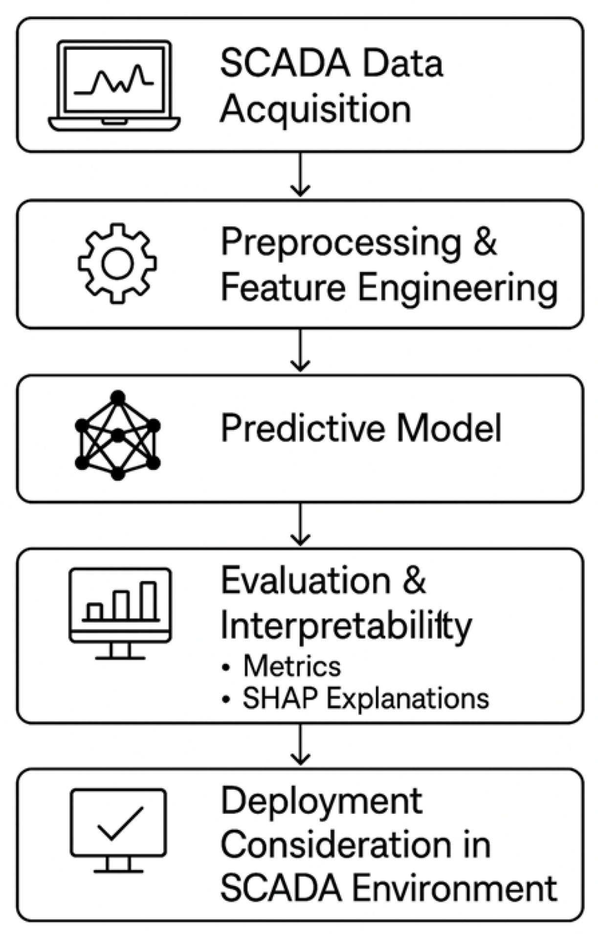
This section outlines the methodology used to investigate predictive maintenance in large-scale bulk-water pump stations. The study follows a structured, five-stage workflow encompassing data acquisition, preprocessing, model development, evaluation, and deployment considerations. The paper adopts a quantitative and applied methodology that blends experimental and exploratory elements. Statistical and machine-learning techniques were applied to historical SCADA data to support three key tasks: anomaly detection, trip-escalation prediction, and RUL estimation.
The approach is experimental in its evaluation of a novel three-layer hybrid model, and exploratory in its goal to uncover fault-relevant signal indicators. As the analysis relied exclusively on secondary operational data collected over extended timeframes, the design enabled longitudinal trend analysis and the identification of precursors to failure events. This methodology addresses the research objectives stated in Section 1, enabling formalised feature extraction, model training, and interpretability analysis based on real-world telemetry.
2.1. Workflow Overview
The methodology is structured into five sequential stages (as shown in Figure 1):
- Data Collection and Acquisition: SCADA data logs from the pump station’s Historian database were retrieved, including sensor readings and event logs over a continuous operational period.
- Data Preprocessing and Feature Engineering: Cleaning, transformation, and extraction of engineering features were performed using statistical and signal-based techniques.
- Model Design: A hierarchical predictive-maintenance architecture was developed, consisting of GRU-based temporal representation learning and anomaly characterisation, supervised trip-escalation prediction using machine-learning classifiers, and remaining useful life (RUL) estimation for short-horizon prognostics.
- Model Evaluation and Validation: Quantitative model performance was assessed using appropriate metrics and cross-validation techniques, with interpretability introduced via explainable AI (XAI) methods.
- Deployment Considerations: A prospective architecture for integrating the predictive framework alongside an existing SCADA environment was defined, including industrial data acquisition, edge-based inference, secure communication, alert management, and operator-facing decision support. The framework was not deployed or tested in a live SCADA environment during the present study.
Figure 1.
Proposed hierarchical GRU-based predictive-maintenance framework.
2.2. SCADA System Data Source
The SCADA system dataset used in this study was obtained from the historian database of a South African bulk-water utility. The utility operates a network of SCADA-enabled pump stations used for real-time monitoring and control of critical water infrastructure. For this study, one pump station was selected as a case site. The station comprises 11 pump sets, of which one pump was selected to provide a controlled single-asset case study and to avoid introducing variability associated with differences in operating profiles between pump sets. Telemetry was recorded at one-minute intervals over one year, resulting in 525,600 timestamped records. Accordingly, the dataset supports chronological evaluation across later operating periods of the selected pump but does not establish generalisation across the station’s other pump sets or across different pumping stations. The collected data included operational parameters such as pressure, flow, vibration, temperature, and electrical current. These measurements form the foundation for both the feature engineering process and the model training stages described in subsequent sections. Instrumentation at the site included suction and discharge pressure transducers, volumetric flow meters, accelerometers mounted on pump and motor bearings, and electrical sensors capturing drive current and shaft speed. All sensors were subject to routine annual calibration by the utility, in compliance with standard operating procedures. Despite calibration protocols, some degree of sensor drift and noise was evident, necessitating downstream filtering and outlier mitigation. Table 1 summarises the sensor categories, labels, units, and descriptions included in the dataset.
Table 1.
Summary of sensor measurements and target variables used in the dataset.
These parameters served as the primary inputs for the fault detection and RUL estimation models. Across the monitoring period, the system exhibited an availability rate of approximately 94%, with fault annotations present in 5.8% of the original records, corresponding to approximately 30,500 timestamped observations. These annotated events formed the basis for both supervised learning and model evaluation tasks. Prior to analysis, all data were anonymised to remove identifiers related to site location, personnel, or equipment serial numbers. Access to the dataset was granted under a formal research agreement with the utility. All activities were conducted in accordance with ethical guidelines for the use of operational data. Confidentiality and data integrity were maintained throughout the project lifecycle.
2.3. Data Preprocessing and Feature Engineering
This phase transformed raw SCADA telemetry into a structured dataset suitable for machine learning analysis. The preprocessing pipeline (as shown in Figure 2) improved data quality, consistency, and temporal representation through four key stages: missing-data imputation, outlier mitigation, noise reduction, and window-based segmentation.
Figure 2.
Data Preprocessing and Feature Engineering.
Approximately 0.6% of sensor readings were missing due to communication or logging faults. Missing intervals shorter than five minutes were imputed using forward filling followed by a three-minute trailing average, calculated from the current value and the preceding two observations. This operation did not use measurements occurring after the current timestamp. Longer gaps were excluded from model training and annotated where appropriate. To preserve temporal continuity while limiting the influence of anomalous measurements, extreme sensor values were clipped using winsorisation at the 1st and 99th percentiles. For each signal x, the lower and upper bounds and , respectively, were applied as given in (1):
This retained approximately 98% of each signal’s observed values while limiting the influence of extreme measurements. Excess kurtosis () was then used to select the level of signal filtering. Channels with were retained without additional filtering to avoid suppressing natural signal variation. Channels with received moderate mean smoothing, while channels with received median filtering because of its greater robustness to isolated extreme observations. The resulting signal profiles were checked through visual inspection of representative segments from each signal type. The kurtosis bands were used as study-specific signal-conditioning categories rather than universal statistical thresholds and were not optimised against downstream model performance. The mean filter used five-point centred windows. The filtered value at time t, therefore, included the two preceding and two subsequent observations, introducing a two-minute delay relative to the current timestamp. For prospective online implementation, preprocessing outputs must be generated using measurements available at the decision time. The three-minute trailing average used for short-gap imputation already satisfies this requirement. The centred mean would either introduce the stated processing delay or require replacement with a trailing or otherwise causal filter.
After cleaning and de-noising, the dataset was segmented into overlapping windows for feature extraction and labelling. The choice of window length (L) and stride (S) was informed by pump-event duration, signal autocorrelation, and a comparative analysis of alternative window configurations. Window lengths of 30, 60, and 120 min were evaluated with overlaps of 25%, 50%, and 75%. Each configuration was assessed using the fault-window coverage rate, defined as the proportion of fault observations represented in at least one fault-labelled window, and the window-level fault rate, defined as the proportion of generated windows labelled as faulty. The results are summarised in Table 2.
Table 2.
Comparison of candidate sliding-window configurations used to select the analysis window and overlap.
The 60-min window with 50% overlap was selected because it achieved 99.0% fault-window coverage while producing a window-level fault rate of 6.1%, close to the underlying fault prevalence. The 30-min configurations provided lower coverage, while the 120-min configurations provided no material improvement over the selected setting. Increasing overlap beyond 50% also generated more highly redundant windows without improving the reported coverage. The selected configuration, therefore, balanced fault representation and overlap while retaining a 30-min update interval.
The sliding-window boundaries are defined by (2), while the total number of windows was calculated using (3).
with min, min, and
where T is the total number of time samples (525,600), and is the total number of generated windows. Each window was assigned two labels. The Binary_Fault label was assigned a value of 1 when more than 30 min within the window were labelled as faulty; otherwise, a value of 0 was assigned. The Multi_Class_Fault label was determined as the modal value of Fault_Type within the window, with deterministic tie-breaking applied where necessary. Partial windows at the beginning and end of the time series were discarded to ensure complete temporal context. Windows containing more than 10% missing or corrupted values were excluded from training. Windows with 10% or fewer missing values retained their computed features and were assigned an auxiliary Missing_Ratio indicator.
2.4. Feature Extraction
With the data segmented into fixed-length labelled windows, each 60-min segment was transformed into a feature vector that (a) summarised raw signal statistics, (b) captured low-frequency temporal variation, and (c) encoded cross-sensor relationships. The extracted features were grouped into three categories.
2.4.1. Time-Domain Features
For each channel, eight time-domain metrics were computed to characterise signal behaviour within a 60-min window. Let , where , denote the one-minute samples in window w, with . The mean was computed as
and represents the baseline signal level, which is useful for detecting gradual changes such as pressure loss or increasing vibration levels preceding a fault. The standard deviation was computed as
and quantifies the magnitude of fluctuations around the mean, thereby providing an indication of unstable or pulsating operating conditions. To characterise extreme values, the minimum, , and maximum, , values within each window were recorded. The difference between these values defines the range, which provides a simple yet effective measure of the signal span. Since extreme values may be influenced by outliers, the interquartile range (IQR) was also computed as
which provides a more robust measure of dispersion than either the standard deviation, , or the range. The shape of the distribution was characterised using skewness:
where positive and negative values indicate asymmetric distributions dominated by high-magnitude spikes and dips, respectively. The excess kurtosis was computed as
and quantifies the heaviness of the distribution tails, thereby helping to identify transient events and spiked behaviour that may not be captured by variance alone. This local kurtosis is distinct from the global used earlier for smoothing decisions. Finally, to detect trends within each window, the slope, m, of the least-squares regression line, , was computed as
where denotes the mean time index within the window. The resulting slope captures gradual temporal trends, such as increasing temperature, rising vibration levels, or declining flow rates, thereby providing sensitivity to progressive changes in system behaviour. These features capture short-term signal variation and longer-term trends within each window.
2.4.2. Frequency-Domain Features
Frequency-domain features were extracted from each vibration channel using a Fast Fourier Transform (FFT). Where necessary, signals were zero-padded or truncated to enable a consistent representation across all 60-min windows. These features capture oscillatory behaviour and spectral characteristics that may be indicative of developing mechanical faults. The spectral centroid was computed as
and represents the centre of mass of the frequency spectrum. Higher values of indicate a greater concentration of spectral energy at higher frequencies, which may reflect changes in machine operating conditions. To quantify fault-related energy concentrations, the band energy was computed over predefined frequency bands, B:
where elevated energy within specific frequency ranges may indicate the presence of abnormal vibration behaviour. The peak frequency was computed as
and identifies the dominant oscillatory component within the window. Finally, the spectral entropy was calculated as
where denotes the normalised spectral magnitude. Spectral entropy quantifies the complexity of the frequency distribution. Lower entropy values indicate spectra dominated by a small number of frequency components, whereas higher values suggest a more distributed spectral composition. These frequency-domain features complement the time-domain measures by representing oscillatory and spectral behaviour within each window.
2.4.3. Cross-Channel and Derived Metrics
In addition to time- and frequency-domain features, a final group of features was derived to capture cross-sensor relationships that reflect the underlying physics of pump operation. These engineered metrics encode fault-relevant interactions that may not be evident from any individual sensor channel. The pressure ratio was computed as
where and denote the mean suction and discharge pressures within window w, respectively. The pressure ratio approximates the hydraulic head across the pump, with decreasing values potentially indicating internal wear, seal leakage, or impeller degradation. The load index was computed as
where and are the mean motor current and shaft speed, respectively. This feature serves as a proxy for mechanical loading, with elevated values potentially indicating cavitation, blockage, or increased mechanical resistance.
The flow-pressure relationship was characterised by fitting a linear regression model:
where m denotes the estimated slope coefficient. Deviations from the nominal slope may indicate hydraulic restrictions, efficiency losses, or abnormal operating conditions.
For thermal monitoring, the thermal differential was defined as
which measures the highest temperature difference between the motor winding and the motor casing. Elevated values of may indicate overheating or insulation degradation.
Finally, the coefficient of variation (CV) of the pumped volume was computed as
where and denote the sample standard deviation and mean, respectively. This feature quantifies relative flow variability, with higher values potentially indicating irregular flow conditions, cavitation, or measurement instability. Overall, these cross-sensor features incorporate physical relationships between measured variables and complement the time- and frequency-domain descriptions of pump behaviour.
2.5. Hybrid Model Architecture
The proposed predictive-maintenance architecture uses a hierarchical three-stage framework to analyse SCADA observations. The first stage uses a GRU network to learn temporal degradation patterns and generate latent representations of pump operating behaviour. The second stage uses these learned representations to predict trip escalation risk using supervised machine-learning classifiers. The third stage estimates RUL for fault trajectories identified as exhibiting progressive degradation. This hierarchical structure enables the framework to capture temporal behaviour, provide early warning of critical trip events, and support maintenance planning through short-horizon prognostics.
2.5.1. Layer 1: GRU-Based Anomaly Detection
A GRU-based encoder was selected due to the temporal nature of SCADA telemetry and the long-horizon degradation behaviour observed during exploratory analysis. Autocorrelation analysis demonstrated that key process variables exhibit slowly decaying temporal dependencies, indicating that degradation patterns develop over extended periods rather than appearing as isolated events. Recurrent neural networks are naturally suited to modelling such sequential behaviour, while GRUs provide a favourable balance between representational capability and computational efficiency when compared with more complex recurrent architectures such as LSTM networks [38].
The anomaly-detection model was implemented as a GRU sequence autoencoder and trained exclusively on healthy windows from the chronological training period. Each input sequence comprised 60 consecutive one-minute observations from the monitored SCADA channels, standardised using statistics derived from the training data. The encoder mapped each input sequence to a 32-dimensional latent representation, while a symmetric GRU decoder reconstructed the original sequence. Model training minimised the mean-squared reconstruction error between the input and reconstructed sequences using the Adam optimiser with a learning rate of . Dropout regularisation and early stopping based on validation loss were applied to reduce overfitting. The resulting encoder was subsequently used to generate latent representations for anomaly scoring and downstream trip-escalation prediction. The architecture and training settings are summarised in Table 3.
Table 3.
GRU sequence-autoencoder configuration and training settings.
The settings in Table 3 specify the final GRU sequence-autoencoder configuration used to obtain the results reported in Section 3.4 and Section 3.5. The selected configuration was not evaluated through an exhaustive architectural sensitivity analysis. Following training, the encoder generated a latent representation, , for each healthy window in the training period. The healthy operating centroid, , was calculated as the component-wise mean of these training embeddings:
where denotes the number of healthy training windows. During inference, each incoming sequence was mapped to a latent representation, , and its anomaly score was defined as the Euclidean distance from the healthy centroid:
Windows with latent representations close to the healthy centroid produced low anomaly scores, while larger centroid distances indicated increasing deviation from learned healthy behaviour. Candidate thresholds were evaluated using anomaly scores and ground-truth labels from the validation period. The threshold that maximised the validation-period F1-score was ; this value was fixed before evaluation on the held-out test period. A window was classified as anomalous according to
where denotes an anomalous window and denotes a window consistent with the learned healthy operating state. The resulting anomaly score and binary anomaly indicator supported Layer 1 fault conditioning and the subsequent trip-escalation stage.
2.5.2. Layer 2: Trip-Escalation Prediction
Layer 2 performs trip-escalation prediction using the latent temporal representations generated by the GRU encoder in Layer 1. Each 60-min sequence is mapped to a 32-dimensional embedding that summarises the temporal behaviour of the monitored SCADA signals. Only fault-conditioned windows identified through Layer 1 are forwarded to the escalation classifier. The objective is to distinguish fault conditions likely to escalate into pump trip events from non-escalating fault behaviour. A calibrated linear SVM and an Extreme Gradient Boosting (XGBoost) classifier were evaluated because of their suitability for compact, imbalanced classification problems.
The Layer 2 prediction target was a binary trip-escalation label indicating whether the fault-conditioned window was associated with a subsequent pump trip within the specified prediction horizon. This hierarchical formulation allows the classifier to focus on escalation risk rather than simultaneously learning general fault detection and trip prediction from the complete imbalanced operating record. Although the calibrated linear SVM achieved marginally higher predictive performance, XGBoost was retained as the corresponding nonlinear classifier because it provided comparable performance within the fault-conditioned embedding space. A separate engineered-feature XGBoost analysis was used to provide the complementary sensor-level interpretation described below.
A complementary SHAP analysis was conducted using the engineered SCADA feature representation for the same fault-conditioned trip-escalation task. This analysis was used to identify the measured variables and derived temporal features associated with escalation risk and should be distinguished from direct interpretation of the individual GRU embedding dimensions. Global rankings summarised the influential variables across the analysed samples, while the beeswarm analysis showed the distribution and direction of their contributions.
In addition to classification outputs, a fault-severity indicator was maintained to monitor degradation trends over time and support progression tracking. Classification probabilities were smoothed across consecutive windows to suppress short-term fluctuations while preserving longer-term degradation behaviour. Sustained increases in escalation risk were used to trigger progression events and initiate the remaining useful life estimation stage described in Section 2.5.3. For progression tracking, denotes the trip-escalation probability produced by the selected Layer 2 classifier for the current fault-conditioned window.
where denotes the fault-severity score at time step t, is the instantaneous classifier output associated with the detected fault condition, is the previous severity estimate, and is the smoothing factor. The coefficient was fixed as a conservative persistence setting and was not selected through a formal sensitivity or optimisation analysis. The reported results, therefore, establish performance for this setting only and do not demonstrate robustness to alternative smoothing coefficients. Under this setting, the current classifier probability contributes 20% of the updated severity score, while 80% is inherited from the preceding smoothed estimate. This reduces the effect of isolated probability spikes and gives greater influence to sustained changes across consecutive windows. If the severity score exceeded a predefined threshold for consecutive windows, a fault-progression event was triggered and passed to the remaining useful life estimation stage.
The dataset was partitioned chronologically into training, validation, and held-out test periods to preserve temporal ordering and provide a realistic assessment of performance on later operating data. The training period was used for model fitting, while validation-period outputs supported hyperparameter selection, early stopping, and decision-threshold calibration. The test period remained excluded from model and threshold selection and was used only for final evaluation. The temporal periods and their methodological roles are summarised in Table 4. Layer-specific evaluation populations were subsequently formed according to the task definition and eligibility criteria of each stage.
Table 4.
Chronological periods used for model development and evaluation.
To mitigate class imbalance within the fault-conditioned Layer 2 training population, the scale_pos_weight parameter in XGBoost was set to the ratio of non-escalating to trip-escalation windows:
where and denote the numbers of non-escalating and trip-escalation windows, respectively, in the Layer 2 training population. The training population contained approximately 12,314 non-escalating windows and 786 trip-escalation windows, corresponding to a positive-class prevalence of approximately 6.0%. The resulting ratio, , was used to set the scale_pos_weight parameter. This fixed class-ratio weighting increased the contribution of the minority trip-escalation class to the XGBoost training objective and was determined exclusively from the training-period Layer 2 labels. The final model was selected using forward-chaining evaluation across the chronological development period. Each fold used an expanding historical training block followed by a later validation block, thereby preserving temporal ordering and preventing future observations from entering the corresponding training block. Model selection considered the macro-averaged F1-score, the area under the receiver operating characteristic curve (ROC-AUC), and precision–recall trade-offs. Hyperparameter optimisation used a predefined search grid, with early stopping based on validation performance to reduce overfitting. The final configuration and decision threshold were fixed before evaluation on the held-out test period.
2.5.3. Layer 3: RUL Estimation
The final layer investigates whether the hierarchical framework can provide an approximate intervention horizon after a developing fault condition has been identified. This conditional regression task is applied only to fault trajectories passed from the preceding anomaly-detection and trip-escalation layers, using the smoothed severity information from Layer 2 together with operational and diagnostic context. The RUL stage is, therefore, evaluated as an exploratory extension of the integrated framework rather than as a standalone prognostic model.
The RUL model was trained using fault trajectories extracted from historical operating data. For each window within a fault trajectory, the prediction target was defined as the remaining time until the onset of a critical event within the trajectory. This formulation enables the model to estimate the available intervention window associated with an escalating fault condition and supports short-horizon prognostic decision-making. The remaining useful life target was expressed in minutes and calculated relative to the endpoint of the identified degradation trajectory.
where t denotes the timestamp of the current window and represents the endpoint of the fault trajectory. To restrict the analysis to a finite pre-event horizon, only windows satisfying 4000 min were retained for training and evaluation. The 4000-min boundary, therefore, defines the scope of the reported RUL model and should not be interpreted as evidence that predictions remain equally reliable throughout this interval.
Each faulty window was represented by a compact set of predictors describing both the current degradation state and its recent progression. The first predictor was the fault-severity score, , defined in (22). This score provides a smoothed representation of the fault probability, thereby reducing short-term fluctuations while preserving longer-term degradation trends. The second predictor was the severity trend, computed as the slope of the severity score over the previous three windows:
where positive values indicate increasing fault severity and may reflect accelerating degradation. The remaining predictors consisted of the values of the ten most influential engineered variables identified through the complementary global SHAP analysis of the fault-conditioned trip-escalation task. These variables provide interpretable physical context and allow the RUL model to incorporate statistical and operational indicators alongside the degradation-dynamics features. An additional predictor was the fault age, defined as the elapsed time since the first anomaly alert within the fault trajectory:
where denotes the timestamp at which the fault was first detected by the anomaly detection and classification layers. This feature provides temporal context regarding fault progression and enables the model to differentiate between newly emerging faults and more mature degradation states. The predictor set, therefore, includes information on anomaly state, degradation dynamics, operational context, and fault history for RUL estimation.
The RUL model used an XGBoost regressor. This allowed non-linear degradation patterns to be modelled using predictors with different scales and statistical characteristics. Training, validation, and test partitions followed the same chronological splits used in the preceding layers, restricted to windows belonging to identified fault trajectories. Hyperparameters were optimised using forward-chaining cross-validation, with the mean absolute error (MAE) used as the primary selection criterion. The final search space consisted of max_depth , learning_rate , n_estimators , and subsample . At inference time, each incoming faulty window produced a feature vector, , that was passed to the trained regressor to estimate the remaining useful life:
To improve temporal consistency and reduce prediction volatility, the estimated RUL values were smoothed using a Kalman filter with a process-noise parameter set to 20. Negative predictions were constrained to zero to ensure physically meaningful outputs. This final layer provides a continuous short-term prognostic estimate that complements the anomaly detection and fault-classification capabilities of Layers 1 and 2 and can be used to inform maintenance scheduling.
2.6. Model Evaluation
Several safeguards were applied to limit information leakage during model development and evaluation. The data were divided chronologically into training, validation, and held-out test periods, ensuring that models were developed using historical observations and evaluated on later operating data. Scaling parameters were estimated from the training data and applied unchanged to the subsequent partitions. Signal-conditioning rules, including the winsorisation and kurtosis-based filtering procedures, were established during development and fixed before final test evaluation. The GRU-based anomaly detector was trained using healthy windows from the training period, while model hyperparameters and decision thresholds were selected using validation-period outputs. The chronologically later test period remained excluded from model and threshold selection and was used only for final performance evaluation. Because consecutive 60-min windows overlapped by 30 min, the final stride preceding each temporal partition boundary was discarded. This prevented windows assigned to adjacent partitions from sharing observations across the boundary.
2.6.1. Layer 1—Unsupervised Anomaly Detection
The anomaly detection layer was evaluated on the test set using the area under the precision–recall curve (PR-AUC), which is well suited to highly imbalanced datasets. Precision and recall were computed on the held-out test period using the anomaly threshold, T, selected by maximising the F1-score on the validation period:
where , , and denote the numbers of true positives, false positives, and false negatives, respectively. The F1-score, which balances precision and recall, was calculated as
2.6.2. Layer 2—Trip-Escalation Prediction
The trip-escalation prediction model was evaluated by selecting a decision threshold, , on the validation set to either maximise the F1-score or minimise a weighted misclassification cost:
where and denote the relative costs associated with false-negative and false-positive predictions, respectively. This validation-stage cost formulation is distinct from the fixed class weighting applied during XGBoost training. The class weight modifies the fitted model by increasing the influence of minority-class training samples, whereas (31) selects the decision threshold applied to the trained classifier. Consequently, the threshold can be adjusted to reflect the relative operational consequences of missed trips and false alarms without retraining the model. Performance on the test set was evaluated using ROC-AUC, PR-AUC, precision, recall, and the F1-score computed at the selected threshold, . Confusion matrices were additionally used to assess the balance between missed trip-escalation windows and false-positive classifications.
Complementary sensor-level interpretability was evaluated using SHAP analysis of the engineered-feature representation within the fault-conditioned prediction context. Global mean absolute SHAP values, , were used to rank influential engineered variables, while the beeswarm analysis showed the distribution and direction of their contributions across the analysed samples.
2.6.3. Layer 3—RUL Estimation
The RUL prediction model was evaluated using the MAE, RMSE, and coefficient of determination (). MAE and RMSE quantify the magnitude of the prediction errors, while indicates how well variation in the observed RUL values is represented by the model. For n test samples with predicted remaining useful lives, , the MAE was computed as
while the RMSE was defined as
where and denote the true and predicted remaining useful life values for sample i, respectively. The coefficient of determination was used alongside these error measures to assess how well the model represented variation in the observed RUL values.
2.7. Deployment and Operational Considerations
The presented framework was evaluated retrospectively using archived SCADA records and was not deployed within a live control environment. The proposed implementation positions the framework as an advisory decision-support system that presents anomaly alerts, trip-escalation probabilities, conditional RUL estimates, and explanatory information to engineering and maintenance personnel. Predictions do not initiate automatic pump-control actions, thereby preserving operator oversight during prospective validation and subsequent operational use. The proposed deployment architecture is illustrated in Figure 3.
Figure 3.
Proposed edge-based architecture for deployment of the predictive-maintenance framework within a SCADA environment.
The architecture acquires sensor and equipment-status data from existing PLC and SCADA systems through industrial interfaces such as OPC-UA, Modbus-TCP, or MQTT. An industrial edge gateway performs preprocessing, hierarchical model inference, and threshold-based alert evaluation. For online operation, preprocessing at the edge gateway must be causal or incorporate an explicitly defined processing delay where centred filtering is retained. MQTT or HTTPS with TLS protection provides secure communication of predictions and associated records to central monitoring and storage services. Local buffering retains recent observations and predictions during temporary communication interruptions, while the central layer supports historical review, dashboard visualisation, traceability, and model and threshold management.
The retrospective experiments were completed without dedicated GPU acceleration and ran in a CPU-based environment. However, deployment-time processor utilisation, model footprint, peak memory demand, storage requirements, and end-to-end inference latency were not formally profiled. These requirements depend on the selected hardware and inference runtime, the number of monitored assets, the retained variables, and the logging policy. Deployment-specific benchmarking is, therefore, required before the computational infrastructure is finalised.
Initial operating thresholds should be selected using temporally separated validation data. The trip-escalation threshold can be selected by maximising the validation-set F1-score or by applying the weighted false-negative and false-positive cost formulation in (31), depending on the relative operational consequences of missed trips and unnecessary interventions. Where class prevalence or operational costs change materially after deployment, recalibration of the decision threshold may be sufficient for short-term adjustment, while retraining with updated or adaptive class weights may be required when the underlying data distribution has changed. Probability smoothing and persistence across consecutive windows provide the first level of protection against isolated alerts. Hysteresis and cooldown logic provide additional protection against repeated alert activation when predictions fluctuate around a decision threshold. Threshold performance should be reviewed against subsequently observed operational events and recalibrated following material changes in operating conditions or prediction calibration. Before operational activation, the framework should undergo shadow-mode evaluation, during which predictions and alerts are recorded without initiating maintenance actions. This would allow false alarms, missed events and warning lead times to be assessed under prospective operating conditions, alongside the stability and practical performance of the system.
3. Results and Discussion
3.1. Exploratory Data Characteristics
The initial analysis of the SCADA dataset revealed significant patterns across sensor domains, with strong inter-variable correlations in process and electrical signals, while vibration and thermal channels exhibited greater independence. For example, flow and discharge pressure showed a Pearson correlation coefficient exceeding , as seen in the correlation heatmap (Figure 4), indicating their shared reflection of hydraulic load conditions. Motor current also demonstrated strong alignment with these variables (), suggesting redundancy within this signal cluster.
Figure 4.
Feature correlation heatmap.
In contrast, vibration data showed substantial signal variance, particularly during active pump operation. Boxplots in Figure 5 illustrate this behaviour, where vibration amplitude distributions displayed long tails and occasional spikes, especially during fault-prone windows. These variations were consistent with the later importance of temporal vibration features in the modelling results.
Figure 5.
Features’ boxplots for raw and normalised data.
The data quality was assessed through missing value analysis. Figure 6 shows the proportion of missing values across channels. Channels with more than 10% missingness were treated explicitly during preprocessing, with short gaps imputed and longer gaps excluded from model development where appropriate.
Figure 6.
Percentage missingness across SCADA sensor channels.
Class balance was examined to assess the challenge presented by the downstream classification tasks. As shown in Figure 7, healthy windows accounted for 87.1% of the windowed dataset, while alarm and trip windows accounted for 7.3% and 5.6%, respectively. Thus, 12.9% of the windows represented non-healthy operating conditions. This class imbalance motivated the use of PR-AUC and F1-score rather than accuracy as the primary classification metrics.
Figure 7.
Distribution of healthy, alarm, and trip conditions.
3.2. Baseline Trip Prediction Performance
Several baseline classifiers were first evaluated for trip prediction. The evaluated models included Logistic Regression, SVM, RF, and XGBoost. Given the low prevalence of trip events within the dataset, model performance was assessed primarily using the PR-AUC, together with precision, recall, and F1-score. These metrics provide a more informative measure of predictive performance than accuracy under severe class imbalance.
The results shown in Table 5 indicate that direct prediction of trip events is challenging. Among the baseline models, the calibrated linear SVM achieved the best overall performance, obtaining a PR-AUC of 0.471 and an F1-score of 0.551. Logistic Regression achieved higher recall (0.618) but substantially lower precision (0.337), resulting in a large number of false alarms. XGBoost provided a more balanced trade-off between precision and recall, although it did not outperform the calibrated SVM. Random Forest exhibited the poorest performance, achieving very high precision but extremely low recall, indicating a tendency to favour the dominant non-trip class and miss critical escalation events.
Table 5.
Performance of baseline classifiers for trip detection.
Figure 8 shows the precision-recall curves for the baseline classifiers under direct trip prediction. Although useful as benchmark references, all baseline approaches exhibited limited capability in identifying rare trip events while simultaneously maintaining acceptable false-alarm rates. This limited baseline performance motivated the use of additional temporal and contextual information in the hierarchical framework.
Figure 8.
Comparison of baseline models for trip detection.
3.3. Enhanced Benchmark Models
A two-stage benchmark was also evaluated for trip prediction. In the first stage, classifiers were trained to identify abnormal operating conditions (faults and alarms), while the second stage predicted escalation from a detected fault condition to a trip event. This approach was motivated by both operational practice and the observed characteristics of the dataset, where fault conditions occur more frequently than trips and, therefore, provide a richer learning signal.
The Stage 1 fault-detection task proved substantially easier than direct trip prediction. Table 6 summarises the Stage 1 results, where several models achieved PR-AUC values close to 0.96, indicating that developing fault conditions exhibit relatively strong and persistent deviations from normal operating behaviour. The Multi-Layer Perceptron (MLP) achieved the highest performance (PR-AUC = 0.965, F1-score = 0.949), closely followed by XGBoost and the calibrated linear SVM. Even the unsupervised autoencoder produced strong fault-detection performance, achieving a PR-AUC of 0.937. Fault conditions, therefore, appear to be well represented in the available SCADA measurements.
Table 6.
Performance comparison of Stage 1 fault detection models.
Trip escalation prediction was considerably more challenging. Despite using a broader benchmark suite, the best-performing models achieved PR-AUC values of approximately 0.54 to 0.55, as shown in Table 7. The calibrated linear SVM produced the highest PR-AUC (0.547), while MLP and XGBoost achieved comparable performance. Decision Trees and Random Forests underperformed, and the unsupervised autoencoder was ineffective as a direct trip-prediction model. These findings suggest that trip events are significantly more difficult to learn than general fault conditions due to their rarity and abrupt onset characteristics.
Table 7.
Performance comparison of Stage 2 trip prediction models.
Figure 9 compares baseline performance of direct trip classification with the two-stage formulation, in which models first predict fault onset before predicting escalation to a trip. Across all evaluated classifiers, the two-stage approach consistently outperformed direct trip prediction. The greatest improvements were observed for tree-based methods, where the use of fault detection as a precursor task substantially improved predictive performance. The comparison suggests that trips are better modelled as the escalation of an existing fault state than as isolated events, which further motivates the hierarchical GRU-based framework.
Figure 9.
Comparison of model performances for trip escalation.
3.4. GRU-Based Anomaly Detection Performance
Despite being trained exclusively on healthy operating windows, the GRU embedding model demonstrated strong fault-detection capability when evaluated against ground-truth labels on the test set. As summarised in Table 8, the GRU centroid distance method achieved a PR-AUC of 0.965 and ROC-AUC of 0.939, with precision, recall, and F1-score all exceeding 0.94. These results indicate that the learned embedding space effectively separates healthy and faulty operating conditions without requiring explicit fault supervision during training.
Table 8.
Performance of the GRU-based anomaly detection model using latent-space centroid distance classification.
Figure 10 presents the precision-recall curve for the GRU embedding model. Precision remained high across a broad range of recall values and only declined near complete recall, a characteristic commonly observed in rare-event detection tasks. The learned latent representation, therefore, retains useful separation between normal and abnormal operating conditions.
Figure 10.
Precision-Recall curve for the GRU embedding model on the test set.
Figure 11 illustrates the distribution of anomaly scores for healthy and faulted operating windows. Healthy samples remained tightly concentrated near zero, while faulty samples formed a distinct higher-distance distribution with a peak around 0.35. A threshold of was selected by maximising the F1-score on the validation period and was then fixed for evaluation on the held-out test period. At this threshold, the clear separation between the healthy and faulty anomaly-score distributions allowed the two operating states to be distinguished reliably.
Figure 11.
Distribution of anomaly scores on the test set.
The GRU-based anomaly detector maintained high detection performance with a relatively low false-alarm rate. The combination of high PR-AUC, clear anomaly-score separation, and strong threshold-dependent performance indicates that the learned latent space provides an effective representation of healthy and faulty operating behaviour. However, fault detection alone is insufficient for operational decision-making, as not all detected faults escalate into pump trip events. While the GRU layer effectively identifies developing degradation, an additional decision layer is required to determine whether a detected fault condition is likely to progress to a critical shutdown event. For this purpose, the latent embeddings generated by the GRU encoder were used as inputs to a supervised trip-escalation classifier.
3.5. Hybrid Trip-Escalation Prediction
Following the benchmark evaluation, the proposed hybrid framework was developed to combine temporal representation learning with supervised trip-escalation prediction. The latent representations generated by the GRU-based anomaly-detection layer were subsequently used as inputs to a supervised trip-escalation classifier. The stages are arranged sequentially so that detected degradation can be assessed for escalation risk before short-horizon RUL estimation is applied. Two candidate classifiers were evaluated, namely a calibrated linear SVM and XGBoost. Following Layer 1 fault conditioning, the held-out Layer 2 evaluation population comprised 2219 windows. Of these, 249 were labelled as positive trip-escalation cases and 1970 as non-escalating cases, corresponding to a positive-class prevalence of 11.2%. This was higher than the approximately 6.0% positive-class prevalence in the training population, reducing the non-escalating-to-escalating ratio from approximately 15.7 during training to 7.91 during testing. The training-derived class weight remained fixed, and the strong held-out performance reported below indicates that this difference did not materially reduce predictive performance during the evaluated test period. Table 9, Figure 12 and Figure 13 report results for this same evaluation population.
Table 9.
Performance of hybrid Layer 2 classifiers for trip prediction.
Figure 12.
Precision–Recall curves for hybrid Layer 2 classifiers.
Figure 13.
Confusion matrices for Layer 2 classifiers.
Both classifiers achieved substantial improvements over the benchmark trip-prediction models presented in Section 3.3. The calibrated linear SVM achieved a PR-AUC of 0.810 and an F1-score of 0.841, while XGBoost achieved a PR-AUC of 0.801 and an F1-score of 0.831. For comparison, the benchmark trip-prediction models reached PR-AUC values of only about 0.55. The calibrated SVM marginally outperformed XGBoost across all primary metrics. However, the performance gap between the two Layer 2 classifiers was small, indicating that both were effective within the fault-conditioned embedding space. The improved performance supports the use of the hierarchical formulation, where temporal representation learning is followed by fault-conditioned escalation prediction. Because the benchmark and hierarchical configurations differ in both representation and gating, the present comparison does not isolate the independent contribution of either component. In addition, the selected GRU configuration was not derived from an exhaustive sensitivity analysis of network depth, hidden-state size, and embedding dimensionality. Its robustness across alternative GRU architectures is, therefore, not established, and systematic optimisation of these parameters may further improve representation quality and downstream trip-escalation performance.
Figure 12 shows that both classifiers maintain precision levels above 0.95 up to approximately 70% recall. Precision then decreases as less certain samples enter the positive class. Given the low prevalence of trip-escalation windows, the resulting precision-recall trade-off remains favourable. The two curves are also closely aligned, although the calibrated SVM performs slightly better across most of the operating range.
The confusion matrices in Figure 13 report the classification outcomes for the same 2219 fault-conditioned test windows used to calculate the threshold-dependent metrics in Table 9. The calibrated SVM correctly identified 182 trip-escalation windows while missing 67, whereas XGBoost correctly identified 180 trip-escalation windows while missing 69. False alarms remained low for both approaches, demonstrating strong discrimination within the fault-conditioned Layer 2 evaluation. The resulting recall and low number of false positives indicate that the hierarchical configuration could be useful for early warning in SCADA-monitored water infrastructure.
Although the calibrated linear SVM achieved marginally higher predictive performance, the difference between the two Layer 2 classifiers was small. XGBoost was retained as the nonlinear embedding-based classifier because it provided comparable performance. The complementary analysis in Section 3.6 uses an engineered-feature representation to provide sensor-level physical interpretation of the same fault-conditioned trip-escalation task.
The comparisons presented here evaluate the complete model configurations rather than the effects of individual architectural components. The observed performance improvement, therefore, reflects the combined contribution of temporal representation learning and fault-conditioned escalation prediction, rather than either component in isolation. A component-wise evaluation using identical samples, labels, chronological partitions, classifier settings, and threshold-selection procedures would be required to distinguish the respective contributions of the GRU representation, engineered features, feature fusion, and Layer 1 conditioning. Repeated forward-chaining evaluations or trajectory-level bootstrap confidence intervals would additionally be required to quantify the variability of the resulting performance differences.
Class imbalance within the fault-conditioned Layer 2 data was addressed through fixed training-time class weighting and validation-based threshold selection. The scale_pos_weight parameter was determined from the ratio of non-escalating to trip-escalation windows in the Layer 2 training population, increasing the influence of the minority trip-escalation class during XGBoost training. The decision threshold was subsequently selected using validation-period predictions and could be adjusted according to the relative operational consequences of missed trips and false alarms.
A more adaptive strategy for addressing class imbalance may be useful where operating conditions or class prevalence differ substantially between assets or change over time. One such approach is the Pareto-optimal adaptive-loss residual shrinkage network [39], in which class-specific misclassification costs are adjusted according to class-frequency differences during training. The method also considers G-mean and multiply-accumulate operations as joint objectives, balancing minority-class recognition against computational complexity, and was evaluated on bearing and milling-cutter datasets under different imbalance ratios. Unlike this approach, the framework used in the present study does not adjust its training loss dynamically or optimise classifier complexity jointly with imbalance-sensitive performance.
3.6. SHAP-Based Interpretation of Trip Escalation
A SHAP analysis of an engineered SCADA feature representation was used to provide sensor-level interpretation alongside the embedding-based Layer 2 evaluation of the same fault-conditioned trip-escalation task. This analysis identifies measured variables and derived temporal features associated with escalation risk and should be interpreted as a sensor-level explanation of the fault-conditioned prediction problem rather than as a direct interpretation of the individual GRU embedding dimensions. Figure 14 presents the global ranking based on mean absolute SHAP values, while Figure 15 shows the distribution and direction of feature-level contributions across individual samples.
Figure 14.
Global ranking of the top 20 individual features for trip-escalation prediction. Bar lengths represent mean absolute SHAP values, while red and blue indicate positive and negative mean signed SHAP contributions to the model output, respectively.
Figure 15.
Global SHAP beeswarm plot for individual-feature contributions to trip-escalation predictions.
At the individual-feature level, the global SHAP ranking in Figure 14 places several vibration-derived variables, particularly temporal features associated with pump non-drive-end vibration, among the most influential predictors of trip escalation. Temperature- and pressure-related variables also appear prominently in the ranking. This feature-level result should be distinguished from the sensor-category aggregation reported in Table 10, which combines the absolute SHAP contributions of all features associated with each sensor domain.
Table 10.
Global sensor-category contributions based on absolute SHAP values.
Figure 15 shows how individual feature values influence trip predictions. The analysis revealed that the model captures complex and context-dependent relationships between vibration, thermal, hydraulic, and electrical variables. Within the vibration domain, temporal characteristics exerted greater influence than absolute vibration magnitudes, indicating that short-horizon changes in vibration behaviour were more informative than static vibration levels.
When the absolute SHAP values were aggregated by sensor category across the complete analysed dataset, temperature measurements accounted for the largest proportion of overall attribution at 80.6%. Vibration contributed 8.2%, followed by pressure at 5.0%, electrical variables at 4.9%, and flow-related variables at 1.3%. This category-level aggregation differs from the individual-feature ranking in Figure 14 and Figure 15 because each category combines the contributions of all associated engineered features. The result indicates that thermal variables provide the dominant aggregated contribution to model behaviour across the broader evaluation dataset. To examine whether these category-level contributions changed as trip activation approached, a complementary temporal analysis was performed for fault windows within approximately ten minutes of trip activation, with the results summarised in Table 11.
Table 11.
Sensor-category contributions based on absolute SHAP values for fault windows within approximately ten minutes of trip activation.
Within this pre-event subset, temporal vibration features became the largest contributor, accounting for 46.4% of the total absolute SHAP attribution, while temperature contributed 40.2% and static vibration features contributed 5.6%. The change from the global category-level result suggests that thermal variables provide broader degradation context across the evaluated data, whereas short-horizon vibration dynamics become increasingly influential as trip activation approaches. Pressure, electrical, and flow variables provide smaller complementary contributions in both analyses.
The SHAP analyses reveal complementary global and pre-event contributions. Temperature provides the largest aggregated attribution across the broader evaluation dataset, while vibration-derived individual features rank prominently and vibration becomes the dominant sensor category immediately before trip activation. This distinction suggests that thermal and vibration measurements contribute differently as a fault progresses towards trip activation. It also provides sensor-level context for the fault-conditioned trip-escalation predictions.
3.7. Remaining Useful Life Estimation
The final stage examined whether the framework could provide an approximate intervention horizon once a developing fault had been identified. RUL was estimated only for fault trajectories identified through the preceding layers and was treated as an exploratory component rather than a standalone prognostic model.
On the test set, the RUL model achieved an MAE of 20.91 min, an RMSE of 63.71 min, and a coefficient of determination () of 0.335. These results should be considered alongside the horizon-dependent behaviour of the point predictions. The model captures the general degradation trend and provides useful near-term risk information. Its predictions, however, are not uniformly reliable across the full 4000-min horizon. The model maintains a relatively conservative estimate of remaining life until degradation becomes sufficiently pronounced to alter the prediction trajectory.
A sorted representation of the test-set predictions is presented in Figure 16. The predicted values broadly follow the overall decline in true RUL and become more accurate as trip occurrence approaches. Predictions made during earlier degradation stages exhibit greater uncertainty and tend to plateau near the maximum prediction horizon. Several factors may contribute to this behaviour. Incipient degradation signatures are weaker and less uniquely associated with an eventual trip when the event remains temporally distant. Variations in pump duty, loading, control actions and degradation pathways can also produce similar sensor states with different times to failure. The min restriction introduces an upper boundary that contributes to the observed ceiling effect, while the limited number and diversity of critical-event trajectories constrain the model’s ability to learn longer-term degradation patterns.
Figure 16.
Sorted view of RUL predictions versus true values with a 25-point moving average.
While the findings indicate the value of the RUL component for short-horizon maintenance support, they also identify several priorities for further development. The effects of GRU depth, hidden-state size, embedding dimensionality, the exponential smoothing coefficient, kurtosis-based filtering boundaries, and the maximum RUL horizon were not evaluated through a complete formal sensitivity analysis. Future work should vary these parameters systematically to determine their influence on representation quality, fault and trip discrimination, false-alert suppression, responsiveness to degradation, computational demand, sample availability, and horizon-specific RUL accuracy. RUL modelling performance should also be evaluated separately across near-, intermediate-, and longer-horizon intervals rather than being interpreted solely through aggregate error measures. Degradation-mode-specific models may reduce uncertainty arising from heterogeneous fault pathways, while sequence-to-sequence architectures could represent the evolution of complete degradation trajectories rather than estimating RUL independently for each window. Incorporating physics-informed indicators, such as hydraulic efficiency, cumulative thermal loading, and vibration-growth characteristics, may also improve the identifiability of degradation during earlier stages. More rigorously calibrated probabilistic or survival-based formulations could provide time-to-event distributions and horizon-specific uncertainty estimates, allowing forecast uncertainty to be incorporated more explicitly into maintenance decisions. Future work should evaluate these developments within the complete hierarchical framework, including their effects on the anomaly-detection and trip-escalation stages.
4. Conclusions
This study developed and evaluated a hierarchical predictive maintenance framework for SCADA-monitored water pump stations, combining GRU-based temporal representation learning, trip-escalation prediction, explainable artificial intelligence, and remaining useful life estimation within a unified workflow. The evaluation used operational telemetry from a bulk-water pumping station and focused on identifying developing degradation before critical failure progression.
The results demonstrated that trip-escalation prediction is substantially more challenging than conventional fault detection. While baseline and benchmark machine-learning models achieved PR-AUC values of approximately 0.47 and 0.55, respectively, the proposed GRU-based hybrid framework achieved PR-AUC values exceeding 0.80. The GRU anomaly-detection layer also achieved a PR-AUC of 0.965 and an F1-score of 0.956, supporting the value of temporal representation learning for characterising degradation behaviour within the hierarchical framework. A complementary engineered-feature SHAP analysis showed that temperature provided the largest aggregated attribution across the broader fault-conditioned dataset, while temporal vibration features became more influential during the immediate pre-trip period. This highlights the complementary roles of thermal degradation context and short-horizon mechanical change in the trip-escalation task. These findings provide physical insight into the degradation process and support the use of sensor-level interpretation alongside the embedding-based predictive framework. The remaining useful life component further extended the framework into short-horizon prognostics, achieving a mean absolute error of 20.91 min while providing useful estimates of maintenance intervention windows preceding critical events. The prognostic component provided complementary short-horizon maintenance information, but its modest , plateauing predictions near the 4000-min boundary, and increased uncertainty during earlier degradation stages limit its use as a precise long-horizon failure-time estimator. Further development could include framework-consistent comparison of alternative prognostic approaches, horizon-stratified and uncertainty-aware evaluation, degradation-mode-specific modelling, and the integration of temporal and physics-informed methods capable of representing complete degradation trajectories.
Within the evaluated single-pump case, the framework provided effective anomaly detection, trip-escalation prediction, and complementary short-horizon prognostic information. However, the presented model was developed and evaluated using only the critical fault and trip events captured in the available dataset, which do not represent the full diversity of degradation modes and trajectories that may occur in operational practice. These findings provide a basis for further development of proactive, data-driven asset management in water-utility infrastructure, with broader applicability requiring validation across additional pumps, pumping stations, operating conditions, failure modes, and prospective deployment environments.
Author Contributions
Conceptualization, L.R., P.N.B. and W.D.; methodology, L.R., P.N.B. and W.D.; software, L.R.; validation, L.R.; formal analysis, L.R.; resources, L.R., P.N.B. and W.D.; data acquisition and curation, L.R.; writing—original draft preparation, L.R., P.N.B. and W.D.; writing—review and editing, L.R., P.N.B. and W.D.; supervision, P.N.B. and W.D.; project administration, L.R. All authors have read and agreed to the published version of the manuscript.
Funding
This research received no external funding.
Data Availability Statement
The raw SCADA telemetry and associated event records were provided by a third-party water utility and are not publicly available because of operational confidentiality and data-privacy restrictions.
Conflicts of Interest
The authors declare no conflicts of interest.
Abbreviations
The following abbreviations are used in this manuscript:
| AI | Artificial Intelligence |
| CMMS | Computerised Maintenance Management System |
| CPU | Central Processing Unit |
| FFT | Fast Fourier Transform |
| FN | False Negative |
| FP | False Positive |
| GRU | Gated Recurrent Unit |
| HMI | Human–Machine Interface |
| HTTPS | Hypertext Transfer Protocol Secure |
| k-NN | k-Nearest Neighbours |
| LSTM | Long Short-Term Memory |
| MAE | Mean Absolute Error |
| ML | Machine Learning |
| MLP | Multi-Layer Perceptron |
| MQTT | Message Queuing Telemetry Transport |
| OPC-UA | Open Platform Communications Unified Architecture |
| PdM | Predictive Maintenance |
| PLC | Programmable Logic Controller |
| PM | Preventive Maintenance |
| PR-AUC | Area Under the Precision–Recall Curve |
| RCM | Reliability-Centred Maintenance |
| RF | Random Forest |
| RM | Reactive Maintenance |
| RMSE | Root Mean Squared Error |
| ROC-AUC | Area Under the Receiver Operating Characteristic Curve |
| RUL | Remaining Useful Life |
| SCADA | Supervisory Control and Data Acquisition |
| SHAP | SHapley Additive exPlanations |
| SVM | Support Vector Machine |
| TLS | Transport Layer Security |
| TP | True Positive |
| XAI | Explainable Artificial Intelligence |
| XGBoost | Extreme Gradient Boosting |
References
- Gopalsamy, T.; Thankappan, V.; Chandramohan, S. An efficient supply management in water flow network using graph spectral techniques. Environ. Sci. Pollut. Res. 2023, 30, 2530–2543. [Google Scholar] [CrossRef] [Scilit]
- Bosserman, B.E.; Ringwood, R.J.; Schmidt, M.D.; Thalhamer, M.G.; Bouthillier, P.H.; Burlingame, R.S.; Charbonneau, A.L.; Peterson, A.W.; Reeser, D.M.; Steiner, J.W.; et al. System Design for Water Pumping. In Pumping Station Design, 3rd ed.; Jones, G.M., Sanks, R.L., Tchobanoglous, G., Bosserman, B.E., Eds.; Butterworth-Heinemann: Oxford, UK, 2008; Chapter 18; pp. 18.1–18.46. [Google Scholar] [CrossRef] [Scilit]
- Garcia-Hernandez, A.; Delgado-Garibay, H.; Rivera Reyes, R.; Martínez, J.L.; Martínez Gomez, L. A New Risk and Reliability Model for Compressor and Pump Installations. In Proceedings of the ASME Turbo Expo 2014: Turbine Technical Conference and Exposition (GT2014), Düsseldorf, Germany, 16–20 June 2014; Volume 3B: Oil and Gas Applications; Organic Rankine Cycle Power Systems; Supercritical CO2 Power Cycles;Wind Energy; American Society of Mechanical Engineers: New York, NY, USA, 2014. [Google Scholar] [CrossRef] [Scilit]
- Department of Water and Sanitation. National Water Resource Strategy: Third Edition (NWRS-3); Department of Water and Sanitation: Pretoria, South Africa, 2023. Available online: https://cer.org.za (accessed on 1 August 2026).
- Rousso, B.Z.; Do, N.C.; Gao, L.; Monks, I.; Wu, W.; Stewart, R.A.; Lambert, M.F.; Gong, J. Transitioning Practices of Water Utilities from Reactive to Proactive: Leveraging Australian Best Practices in Digital Technologies and Data Analytics. J. Hydrol. 2024, 641, 131808. [Google Scholar] [CrossRef] [Scilit]
- Kamil, A.I.M.; Fathi, M.S.; Aziz, Z.; Ismail, N.A.A. Digital twin framework for addressing water management challenges in Malaysia. In Proceedings of the Institution of Civil Engineers-Municipal Engineer; Emerald Publishing Limited: Leeds, UK, 2025; pp. 1–15. [Google Scholar] [CrossRef] [Scilit]
- Delnaz, A.; Nasiri, F.; Li, S.S. Asset Management Analytics for Urban Water Mains: A Literature Review. Environ. Syst. Res. 2023, 12, 12. [Google Scholar] [CrossRef] [Scilit]
- Latifi, M.; Sharafodin, S.; Gheibi, M. Predictive Rehabilitation of Clean Water Customer Connections Leveraging Machine Learning Algorithms and Failure Time Series Data. Water 2026, 18, 110. [Google Scholar] [CrossRef] [Scilit]
- Thomas, D.; Weiss, B. Maintenance Costs and Advanced Maintenance Techniques in Manufacturing Machinery: Survey and Analysis. Int. J. Progn. Health Manag. 2021, 12, 1–13. [Google Scholar] [CrossRef] [Scilit]
- Johannesburg Water. Rand Water Planned Maintenance: Customers Fed by Eikenhof Pumpstation. Available online: https://johannesburgwater.co.za/rand-water-planned-maintenance-customers-fed-by-eikenhof-pumpstation/ (accessed on 1 August 2026).
- City of Tshwane. Bronkhorstspruit Water Treatment Plant Operating at Low Capacity–City of Tshwane. Available online: https://www.tshwane.gov.za/?p=51483 (accessed on 1 August 2026).
- Steger, P.; Pierce, D.; Dunlap, S. LifT Stations: You Can’t Manage What You Can’t Measure: Applying Realtime Analytics for Asset Management. In Proceedings of the 91st Annual Water Environment Federation Technical Exhibition and Conference (WEFTEC 2018); Water Environment Federation: Alexandria, VA, USA, 2019; pp. 5359–5368. [Google Scholar]
- Hector, I.; Panjanathan, R. Predictive Maintenance in Industry 4.0: A Survey of Planning Models and Machine Learning Techniques. PeerJ Comput. Sci. 2024, 10, e2016. [Google Scholar] [CrossRef] [Scilit]
- Zhu, T.; Ran, Y.; Zhou, X.; Wen, Y. A Survey on Intelligent Predictive Maintenance (IPdM) in the Era of Fully Connected Intelligence. IEEE Commun. Surv. Tutor. 2025, 28, 633–671. [Google Scholar] [CrossRef] [Scilit]
- Mallioris, P.; Aivazidou, E.; Bechtsis, D. Predictive Maintenance in Industry 4.0: A Systematic Multi-Sector Mapping. CIRP J. Manuf. Sci. Technol. 2024, 50, 80–103, Erratum in CIRP J. Manuf. Sci. Technol. 2024, 55, 420. [Google Scholar] [CrossRef] [Scilit]
- Brad, S.; Murar, M.; Vlad, G.; Brad, E.; Popanton, M. Lifecycle Design of Disruptive SCADA Systems for Waste-Water Treatment Installations. Sustainability 2021, 13, 4950. [Google Scholar] [CrossRef] [Scilit]
- Dwarakanath, B.; Kalpana Devi, P.; Ranjith Kumar, A.; Metwally, A.S.M.; Ashraf, G.A.; Thamineni, B.L. Smart IoT-Based Water Treatment with a Supervisory Control and Data Acquisition (SCADA) System Process. Water Reuse 2023, 13, 411–431. [Google Scholar] [CrossRef] [Scilit]
- Zamikhovskyi, L.; Nykolaychuk, M.; Levytskyi, I. Organizing the Automated System of Dispatch Control over Pump Units at Water Pumping Stations. East.-Eur. J. Enterp. Technol. 2024, 5, 61–75. [Google Scholar] [CrossRef] [Scilit]
- Pinzón, J.D.; Osorno, T.; Mola, J.A.; Valencia, A. Real-Time Health Condition Monitoring of SCADA Infrastructure of Power Transmission Systems Control Centers. In Proceedings of the 2020 IEEE PES Transmission & Distribution Conference and Exhibition–Latin America (T&D LA), Montevideo, Uruguay, 28 September–2 October 2020; pp. 1–6. [Google Scholar] [CrossRef] [Scilit]
- Moleda, M.; Momot, A.; Mrozek, D. Regression Methods for Detecting Anomalies in Flue Gas Desulphurization Installations in Coal-Fired Power Plants Based on Sensor Data. In Computational Science–ICCS 2020; Lecture Notes in Computer Science; Springer: Cham, Switzerland, 2020; Volume 12141, pp. 316–329. [Google Scholar] [CrossRef] [Scilit]
- Bui, M.T.; Yáñez-Godoy, H.; Elachachi, S.M. Assessment of the Implications and Challenges of Using Artificial Intelligence for Urban Water Networks in the Context of Climate Change When Building Future Resilient and Smart Infrastructures. J. Pipeline Syst. Eng. Pract. 2025, 16, 1. [Google Scholar] [CrossRef] [Scilit]
- Carvalho, T.P.; Soares, F.A.A.M.N.; Vita, R.; Francisco, R.P.; Basto, J.P.; Alcalá, S.G.S. A Systematic Literature Review of Machine Learning Methods Applied to Predictive Maintenance. Comput. Ind. Eng. 2019, 137, 106024. [Google Scholar] [CrossRef] [Scilit]
- Khan, U.; Cheng, D.S.; Setti, F.; Fummi, F.; Cristani, M.; Capogrosso, L. A Comprehensive Survey on Deep Learning-Based Predictive Maintenance. ACM Trans. Embed. Comput. Syst. 2025, 25, 1. [Google Scholar] [CrossRef] [Scilit]
- Bris-Peñalver, F.J.; Verdecia-Peña, R.; Alonso, J.I. A Survey of AI-Enabled Predictive Maintenance for Railway Infrastructure: Models, Data Sources, and Research Challenges. Sensors 2026, 26, 906. [Google Scholar] [CrossRef] [Scilit]
- Baird, G.M. New U.S. and International Water Main Break Studies: More Detailed Pipe Analysis but What Are We Doing with the Data? In Pipelines 2020; American Society of Civil Engineers: Reston, VA, USA, 2020; pp. 316–325. [Google Scholar] [CrossRef] [Scilit]
- Castle, P.; Ham, J.; Hodkiewicz, M.; Polpo, A. Interpretable Survival Models for Predictive Maintenance. In Proceedings of the 30th European Safety and Reliability Conference and the 15th Probabilistic Safety Assessment and Management Conference (ESREL2020 PSAM15), Venice, Italy, 1–5 November 2020; pp. 3392–3399. [Google Scholar] [CrossRef] [Scilit]
- Taiwo, R.; Shaban, I.A.; Ahmad, T.; Zayed, T. Big Data-Driven Prediction of Watermain Failures in Semi-Tropical Regions: Case Study of Hong Kong’s Distribution Network. Autom. Constr. 2025, 175, 106159. [Google Scholar] [CrossRef] [Scilit]
- Mahale, Y.; Kolhar, S.; More, A.S. Enhancing Predictive Maintenance in Automotive Industry: Addressing Class Imbalance Using Advanced Machine Learning Techniques. Discov. Appl. Sci. 2025, 7, 4. [Google Scholar] [CrossRef] [Scilit]
- Nieminen, W.; Gebreweld, H.; Liuha, A.; Nissinen, M.; Verdugo, M.; Mikkola, A.; Kutvonen, A. Synthetic Data for Predictive Maintenance: A Systematic Review and Framework for Industry 4.0 Applications. J. Intell. Manuf. 2026. [Google Scholar] [CrossRef] [Scilit]
- Ucar, A.; Karakose, M.; Kırımça, N. Artificial Intelligence for Predictive Maintenance Applications: Key Components, Trustworthiness, and Future Trends. Appl. Sci. 2024, 14, 898. [Google Scholar] [CrossRef] [Scilit]
- Sinha, S.K.; Bell, G. National Water Pipeline Infrastructure Database PIPEiD. In Pipelines 2022; American Society of Civil Engineers: Reston, VA, USA, 2022; pp. 70–80. [Google Scholar] [CrossRef] [Scilit]
- Deloitte. AI for Water Supply Systems: Planning for the Future. Case Study: MPWiK Wrocław × Deloitte–Predictive Maintenance. Available online: https://www.deloitte.com/pl/pl/services/consulting/case-studies/AI-for-water-supply-systems-planning-for-the-future.html (accessed on 1 August 2026).
- Hexagon. How a Leading Water Utility Leverages HxGN EAM for Intelligent Networks and Predictive Maintenance. Available online: https://aliresources.hexagon.com/operations-maintenance/how-a-leading-water-utility-leverages-hxgn-eam-for-intelligent-networks-and-predictive-maintenance-2 (accessed on 1 August 2026).
- Sunal, C.E.; Dyo, V.; Velisavljevic, V. Review of Machine Learning Based Fault Detection for Centrifugal Pump Induction Motors. IEEE Access 2022, 10, 71344–71355. [Google Scholar] [CrossRef] [Scilit]
- Ma, W.; Ma, S.; Zou, Z.; Fu, B.; Ma, J.; Liu, J.; Zhang, Q. Literature Review on Fault Mechanism Analysis and Diagnosis Methods for Main Pump Systems. Machines 2025, 13, 1000. [Google Scholar] [CrossRef] [Scilit]
- Shaikh, F.; Ahmed, B.S.; Swerin, A. Unsupervised Detection of Faults in Industrial Pumps from Multivariate Time Series. Mach. Learn. Appl. 2025, 22, 100784. [Google Scholar] [CrossRef] [Scilit]
- Adaika, H.; Tir, Z.; Sahraoui, M.; Laadjal, K. PumpSpectra: An MCSA-Based Platform for Fault Detection in Centrifugal Pump Systems. Sensors 2025, 25, 6916. [Google Scholar] [CrossRef] [Scilit]
- Mirzaei, S.; Kang, J.-L.; Chu, K.-Y. A Comparative Study on Long Short-Term Memory and Gated Recurrent Unit Neural Networks in Fault Diagnosis for Chemical Processes Using Visualization. J. Taiwan Inst. Chem. Eng. 2022, 130, 104110. [Google Scholar] [CrossRef] [Scilit]
- Yu, Y.; Guo, L.; Gao, H.; Liu, Y.; Feng, T. Pareto-Optimal Adaptive Loss Residual Shrinkage Network for Imbalanced Fault Diagnostics of Machines. IEEE Trans. Ind. Inform. 2022, 18, 2233–2243. [Google Scholar] [CrossRef] [Scilit]
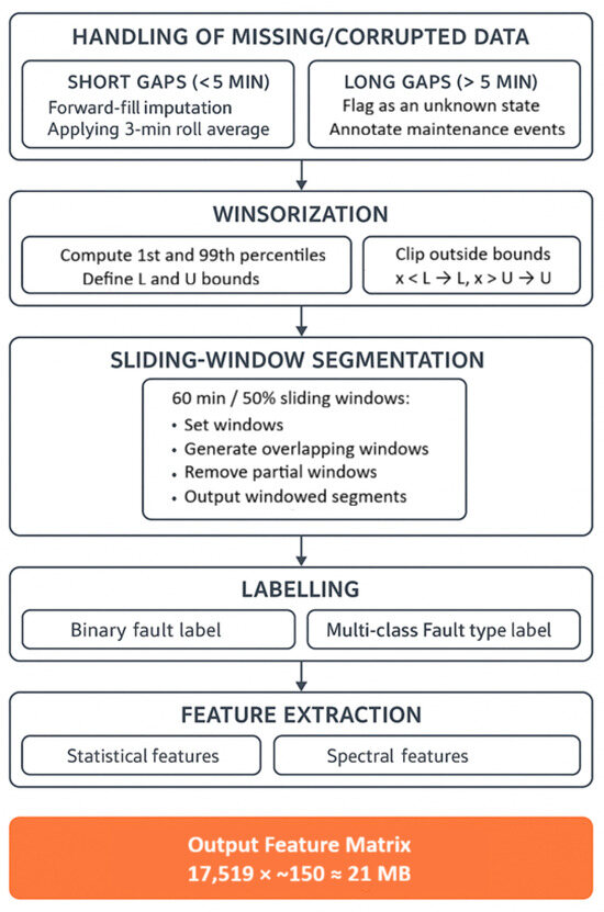
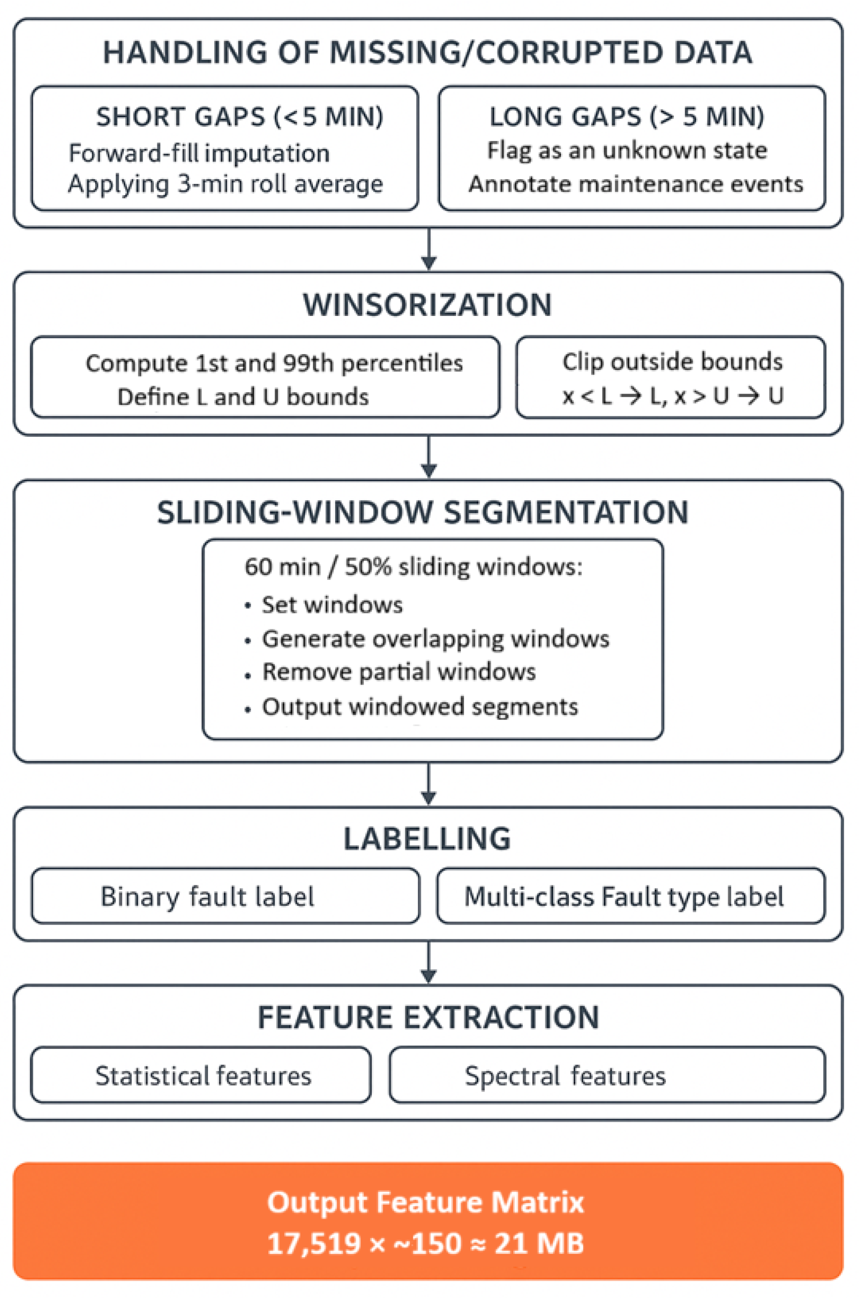
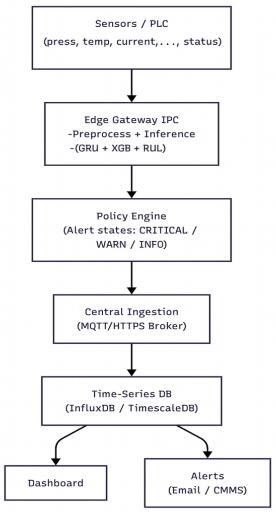
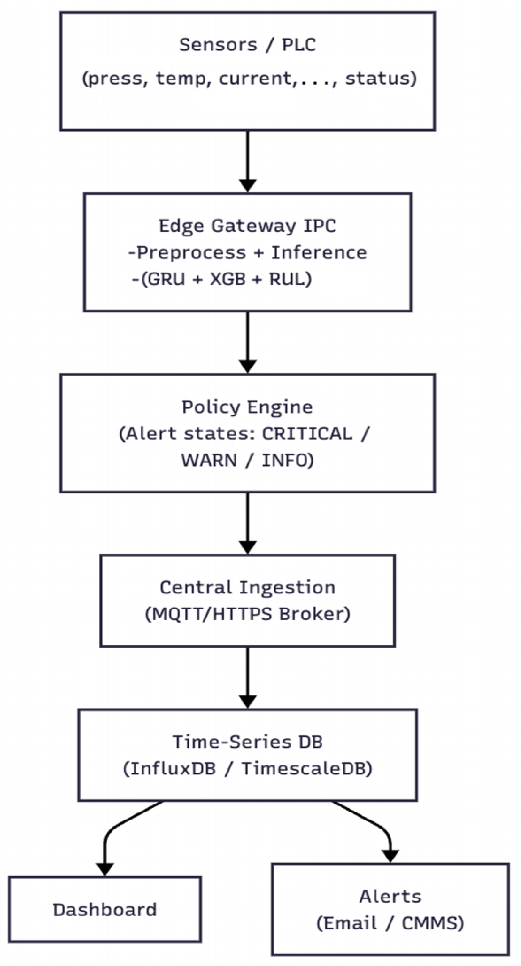
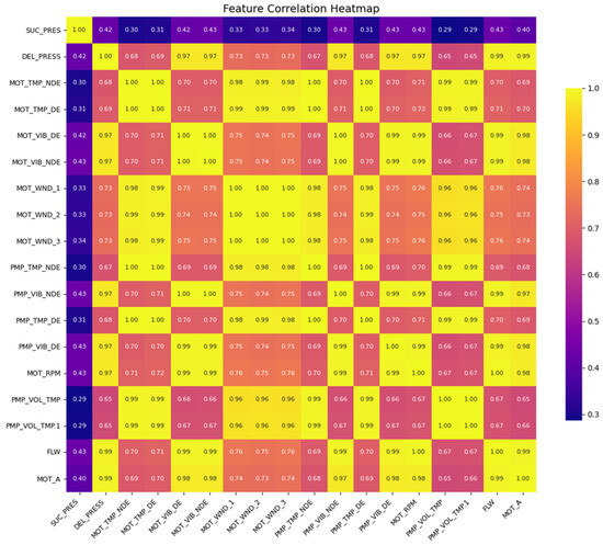
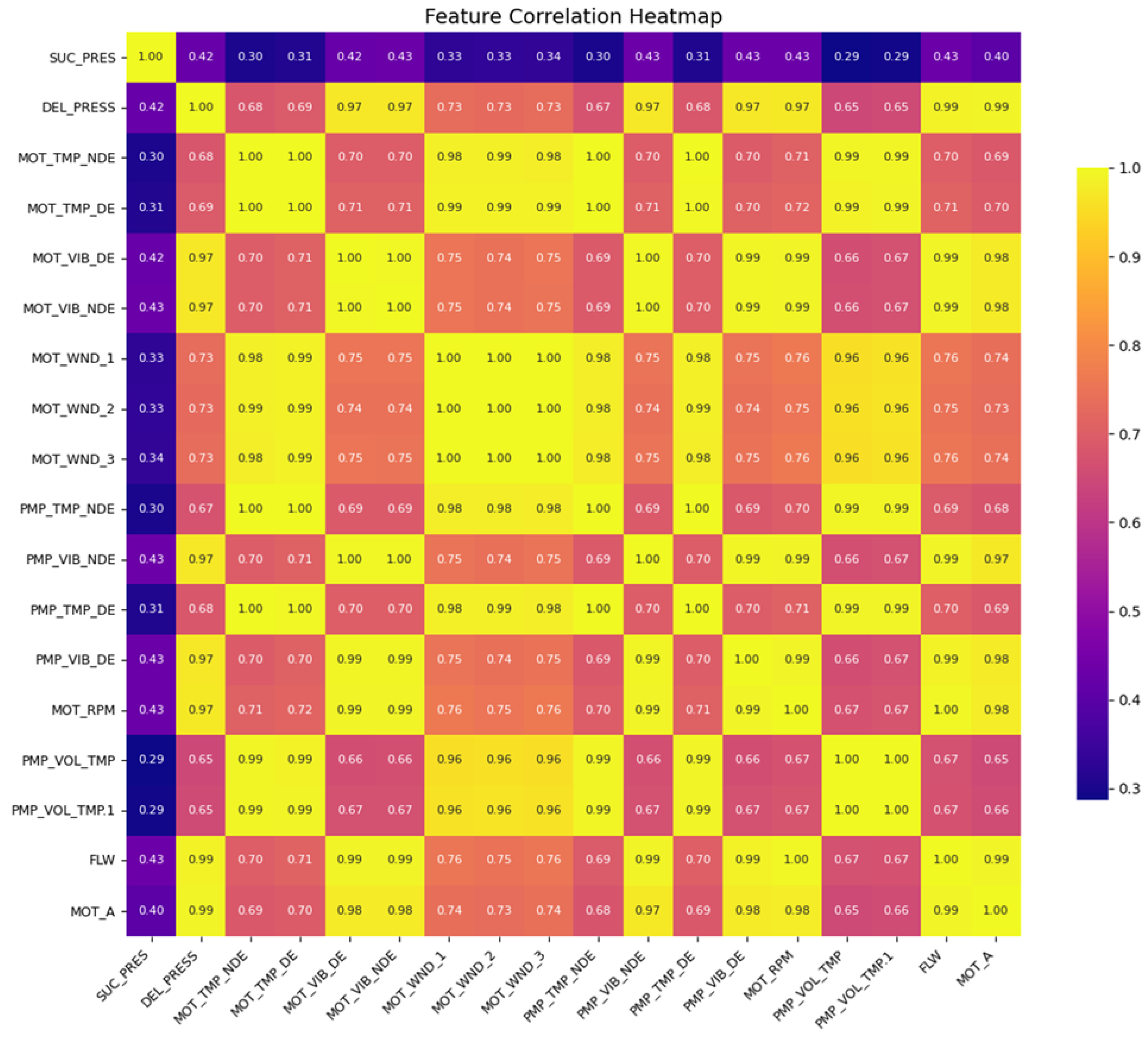
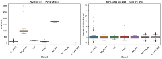
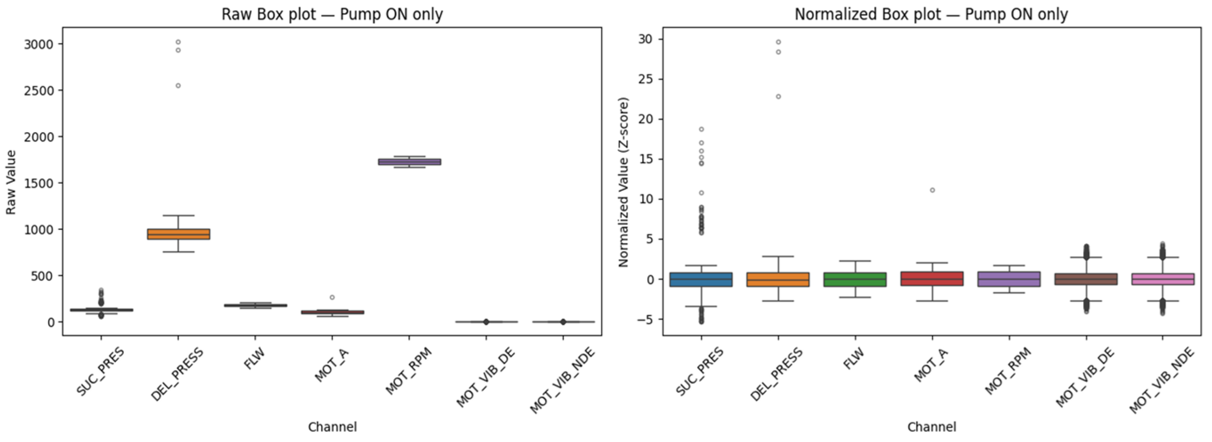
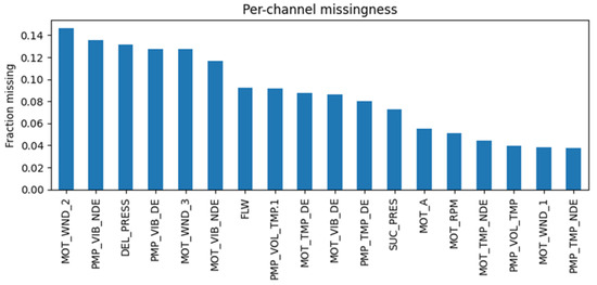
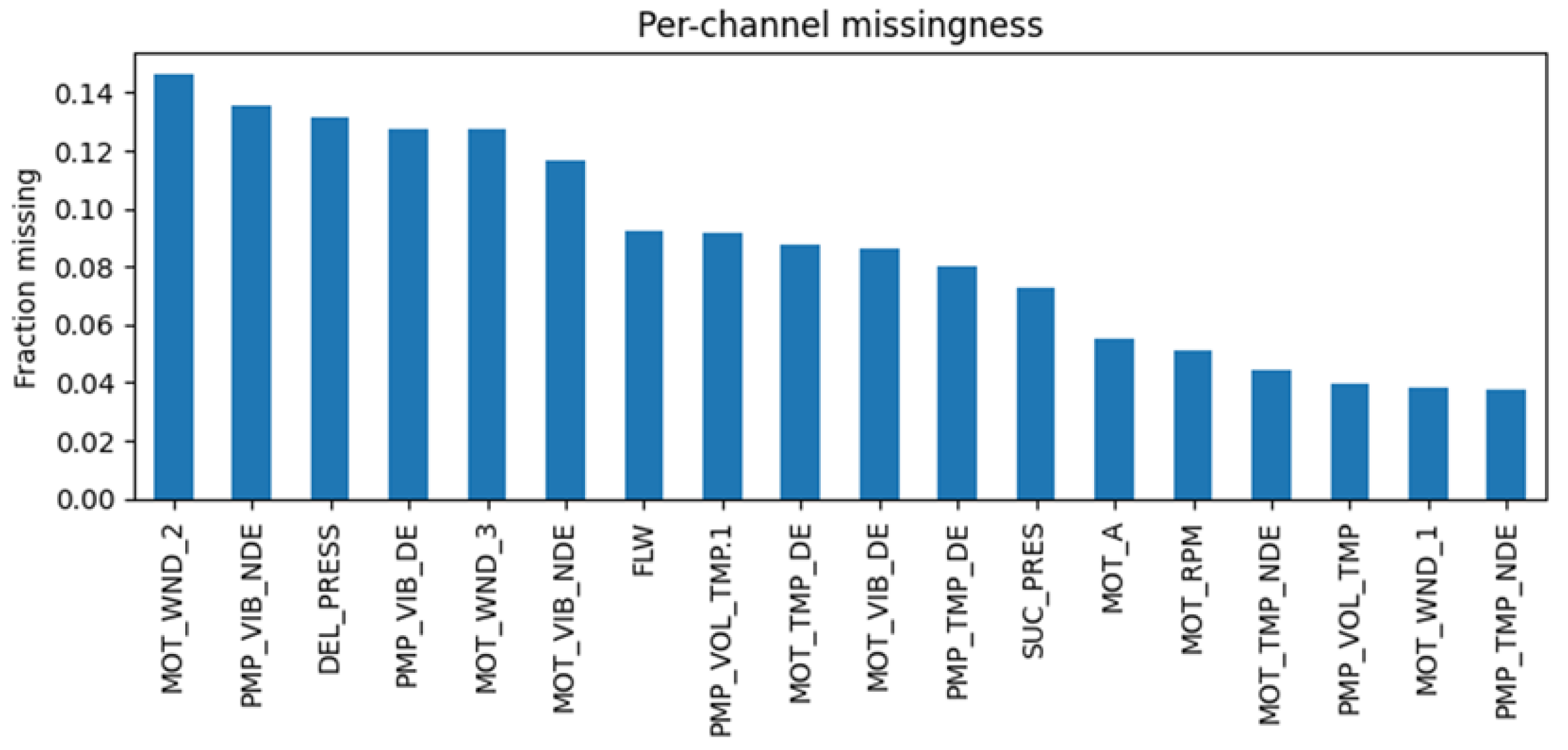
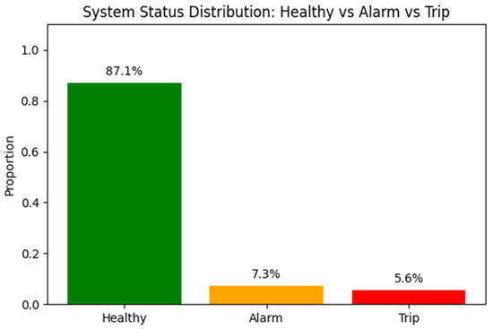
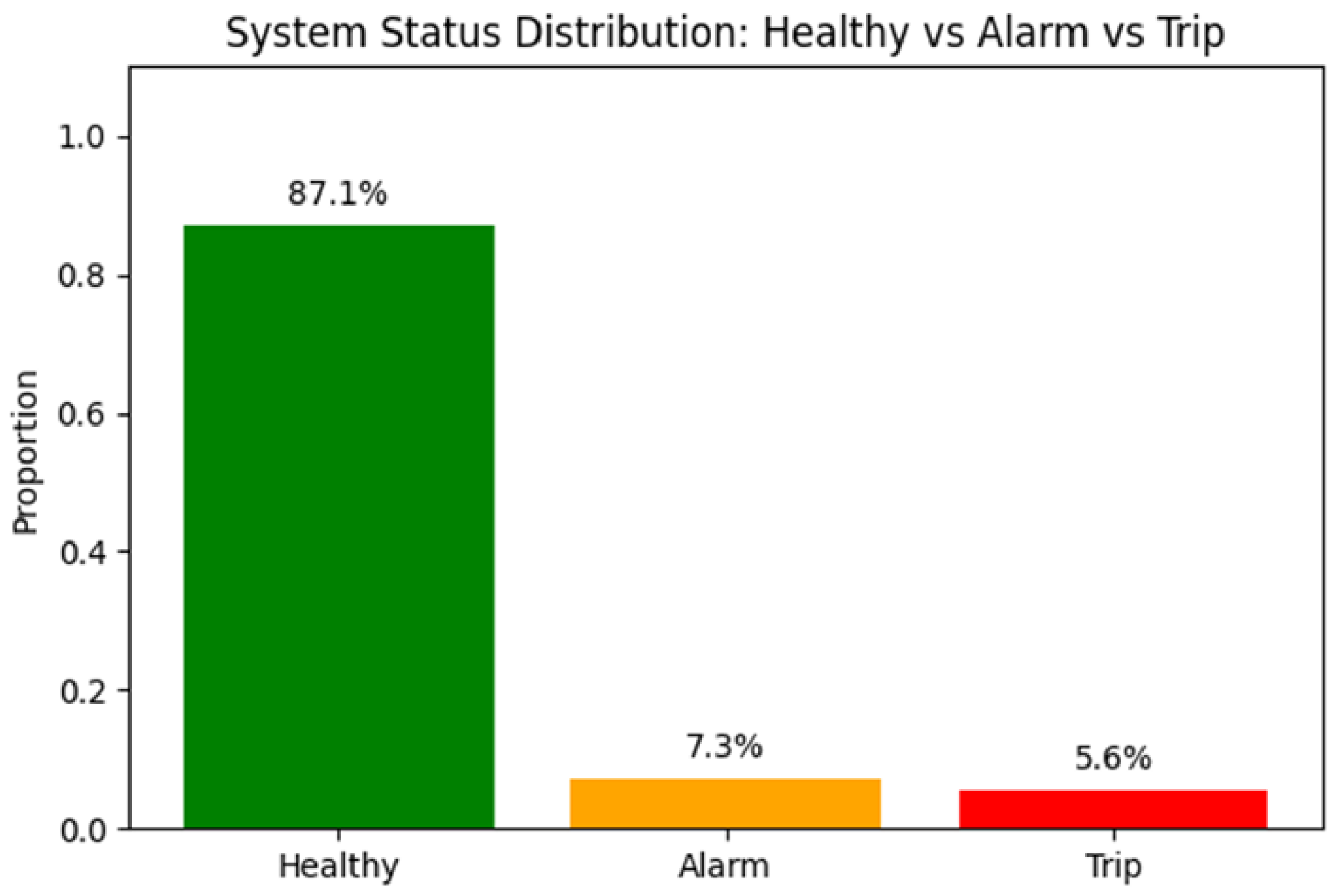
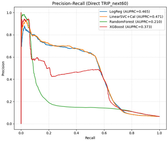
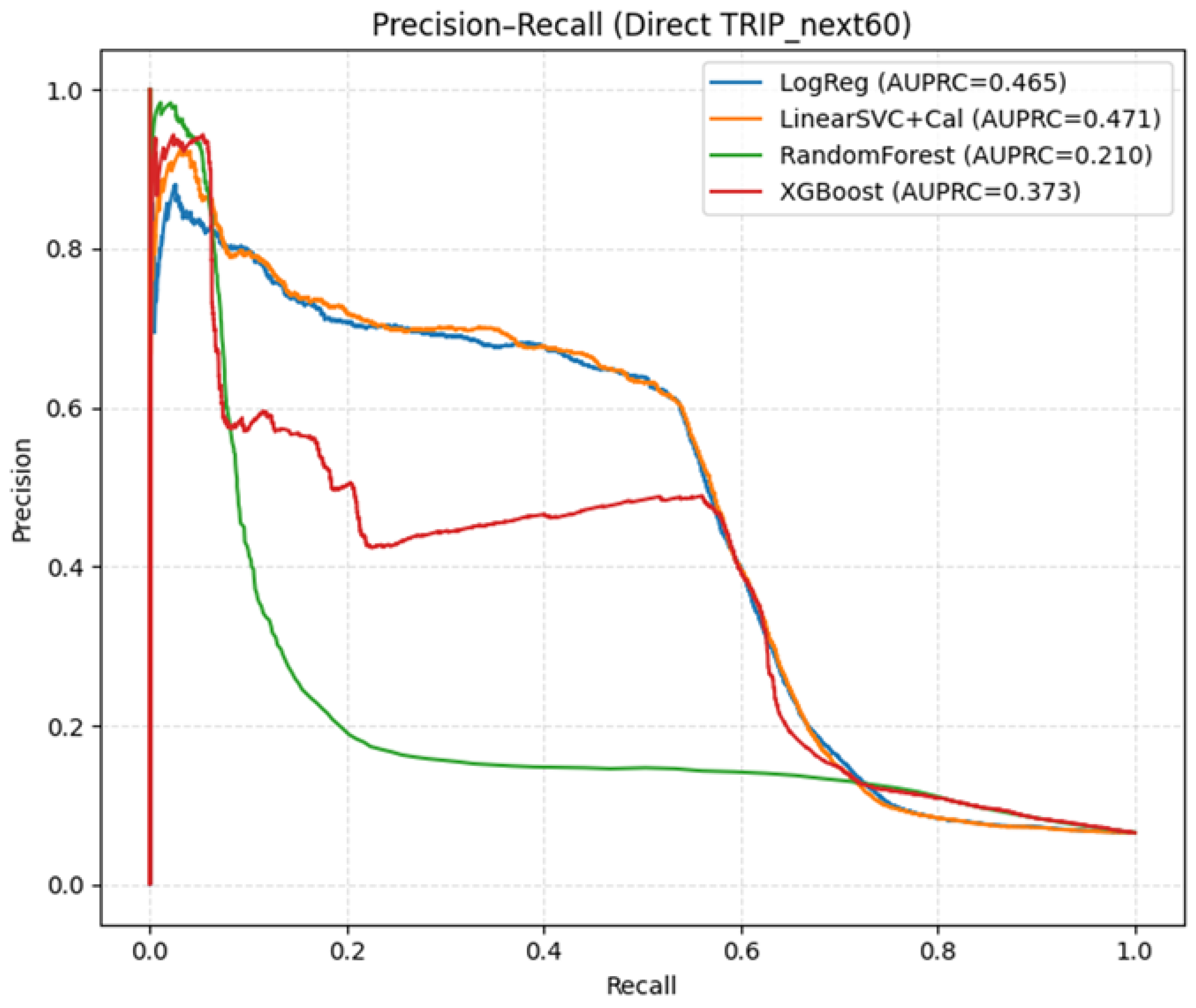
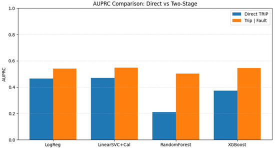
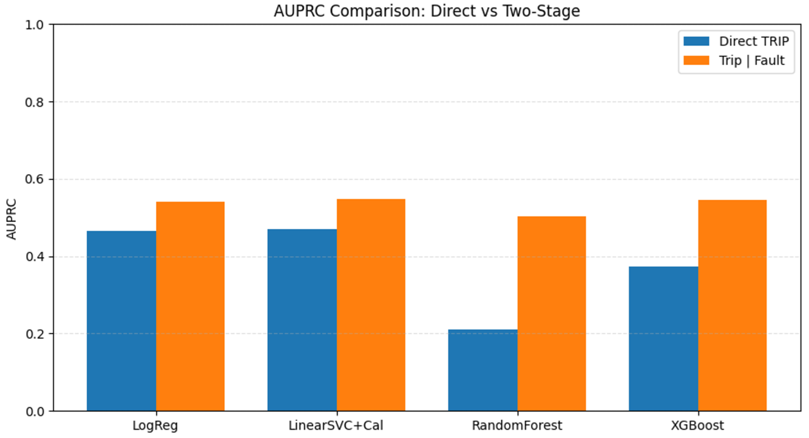
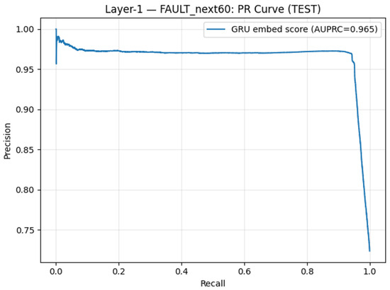
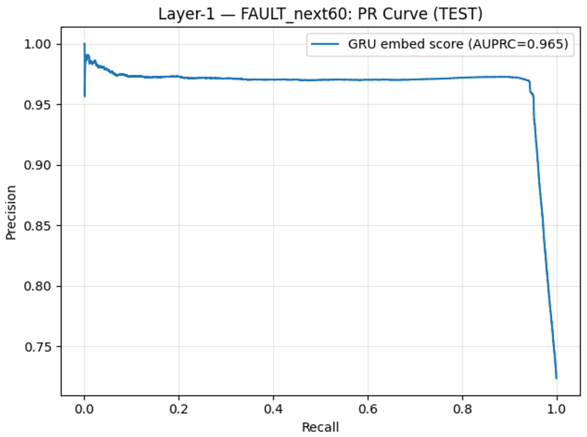
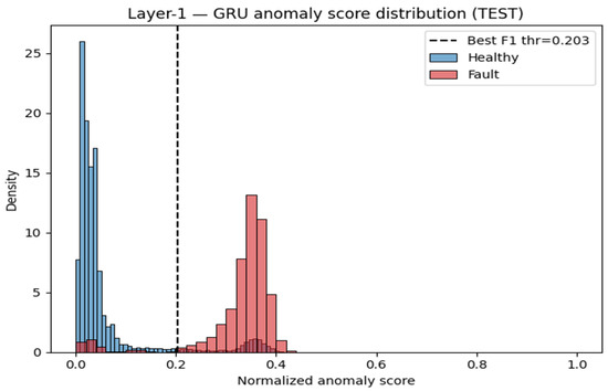
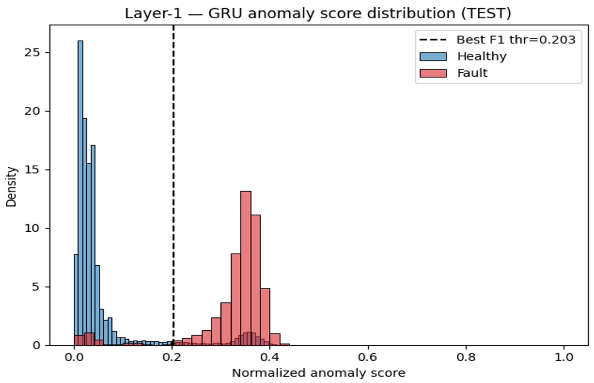
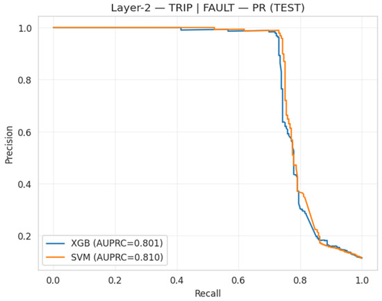
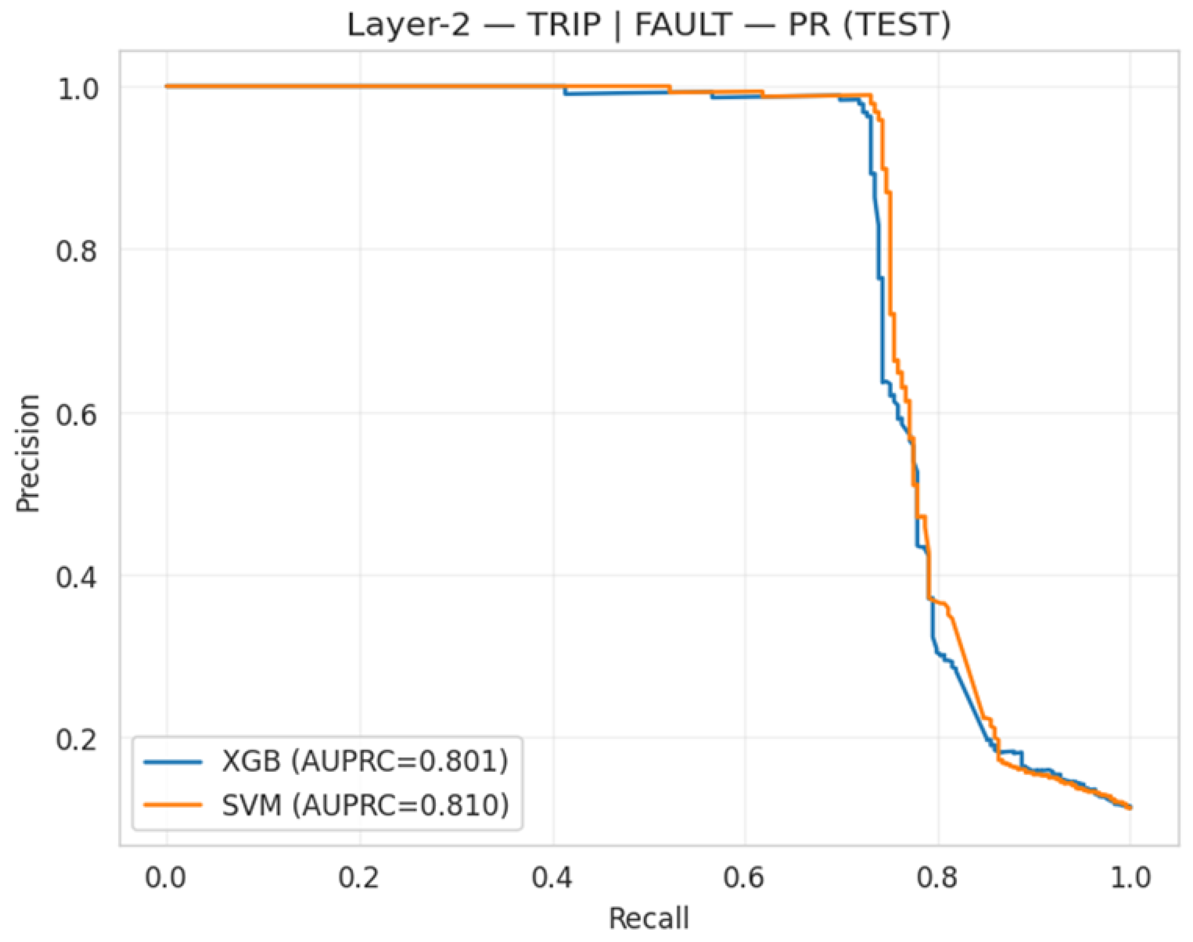
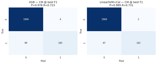
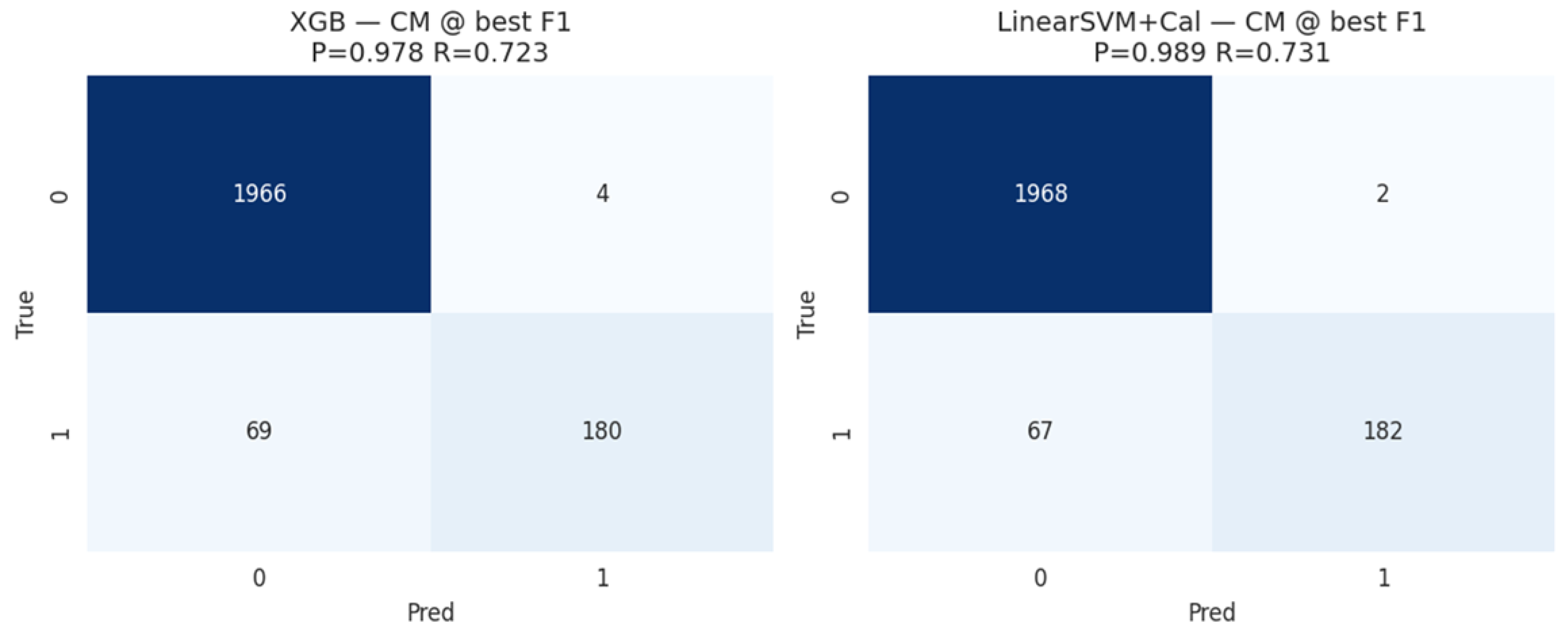
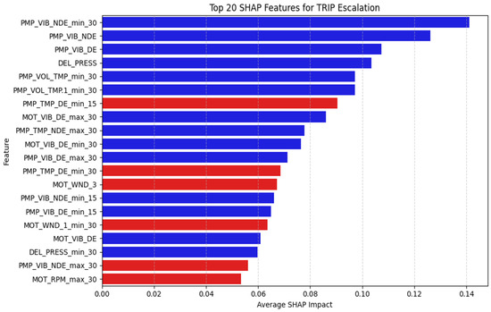
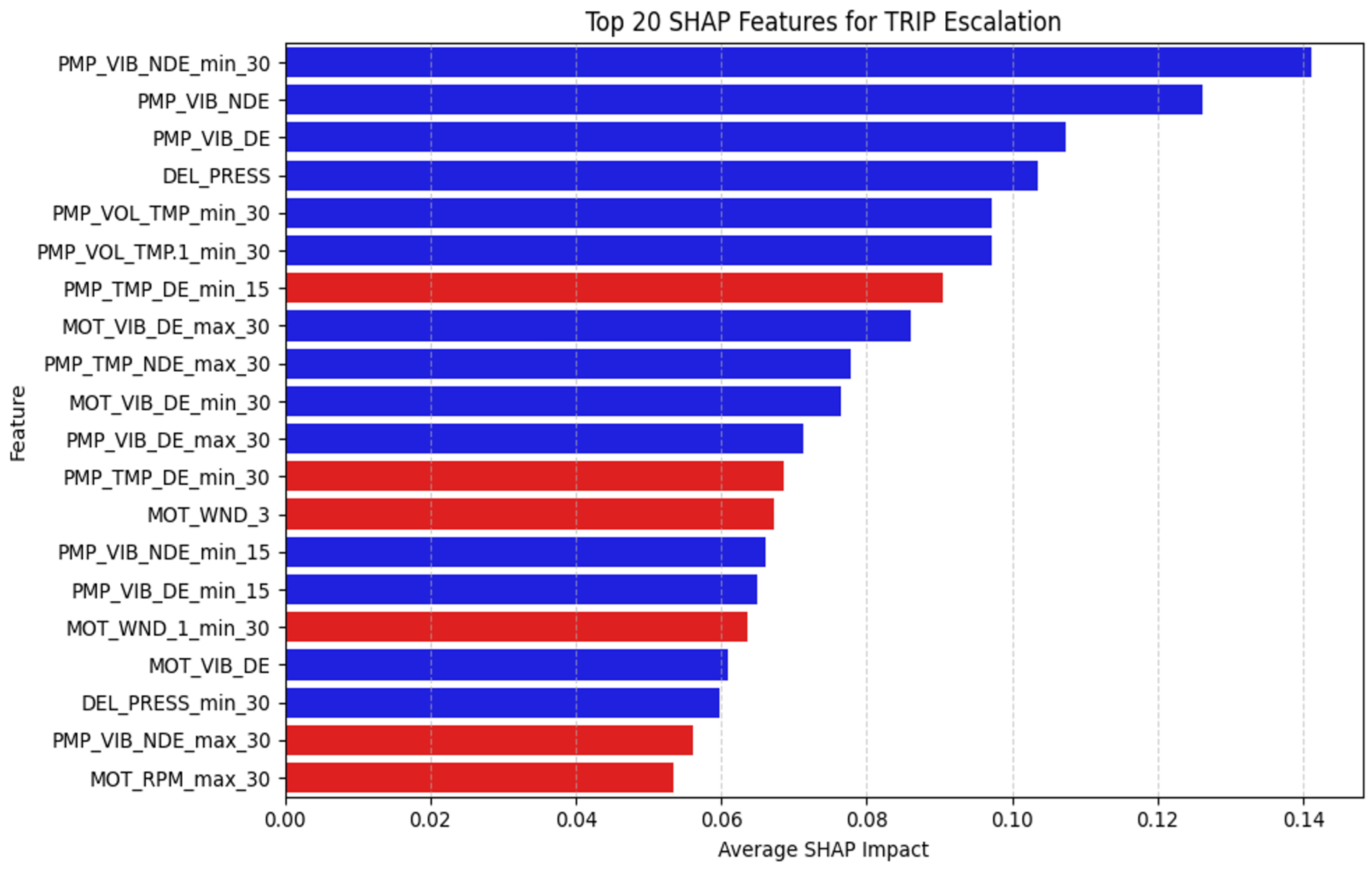
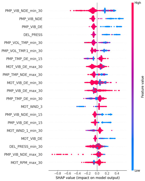
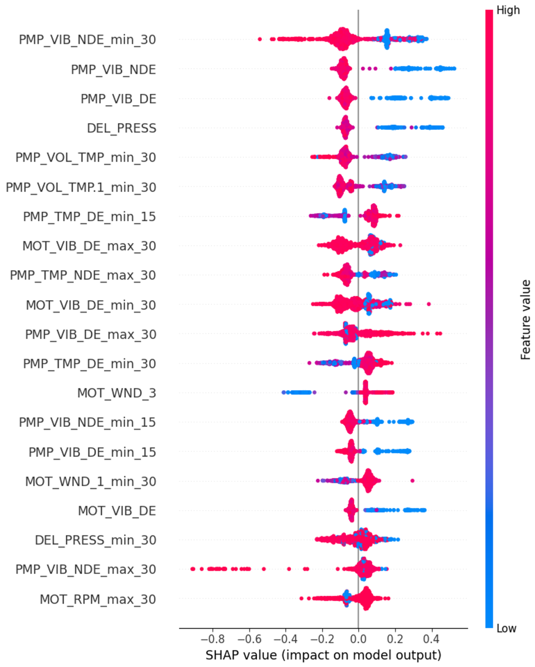
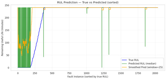
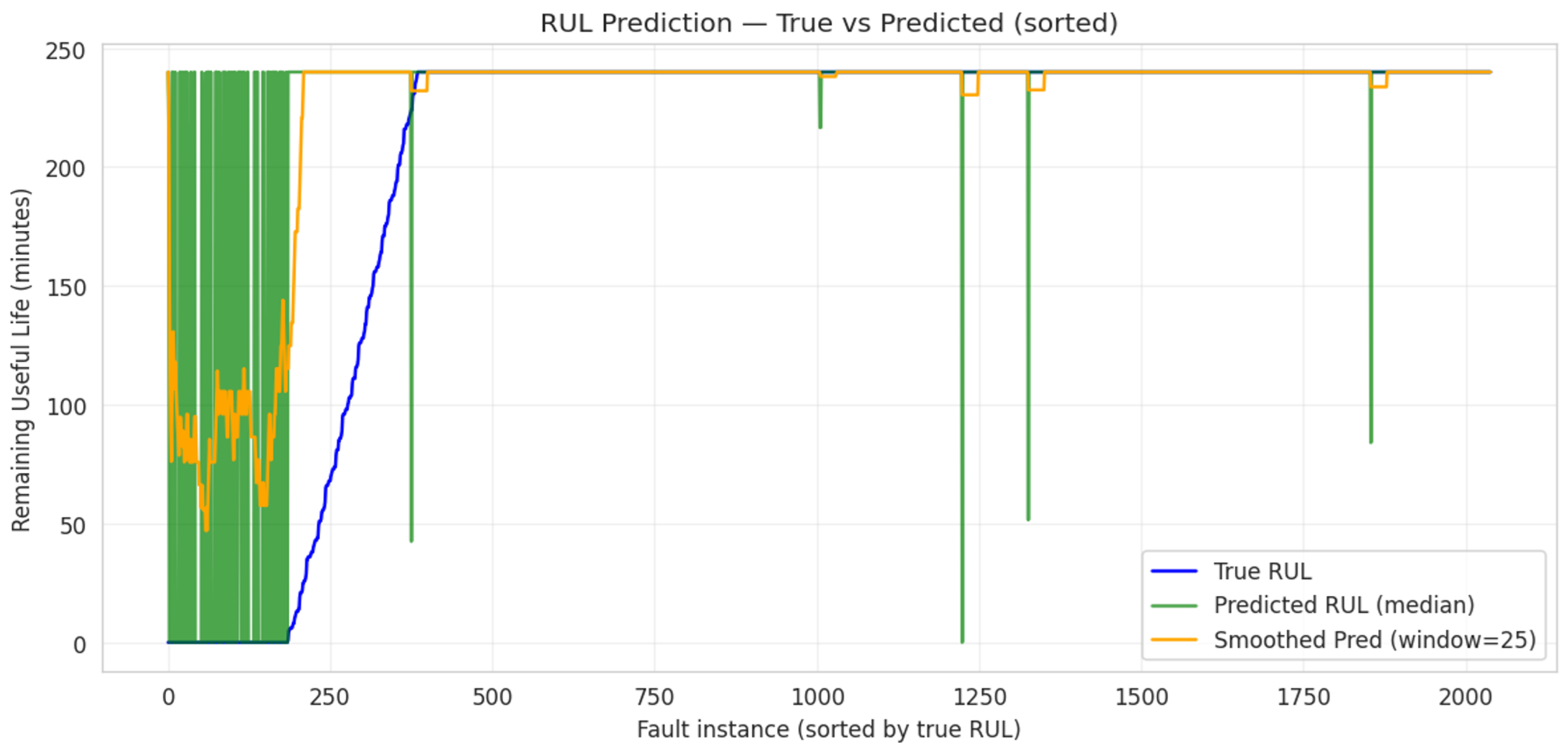

Disclaimer/Publisher’s Note: The statements, opinions and data contained in all publications are solely those of the individual author(s) and contributor(s) and not of MDPI and/or the editor(s). MDPI and/or the editor(s) disclaim responsibility for any injury to people or property resulting from any ideas, methods, instructions or products referred to in the content. |
© 2026 by the authors. Licensee MDPI, Basel, Switzerland. This article is an open access article distributed under the terms and conditions of the Creative Commons Attribution (CC BY) license.