


Abstract
In this paper, we investigate a one-dimensional tree-structured Timoshenko beam system composed of three beams with boundary feedback controls and derive its explicit exponential decay rate. We first formulate a dynamic model incorporating end loads, boundary feedback, and multi-beam coupling relationships. Then, by applying Lyapunov’s method, we construct an energy functional suitable for this coupled system. This study not only provides rigorous proof of the exponential stability of the coupled Timoshenko beam system, but also yields an explicit decay rate under prescribed conditions. Our results offer theoretical support and a quantitative foundation for vibration suppression of multi-beam-coupled flexible structures.
Keywords:
partial differential equations; timoshenko beam; boundary control; tree-structured network; exponential decay; decay rate MSC:
35Q93; 35B40; 93D15; 93D20
1. Introduction
The Timoshenko beam theory provides a fundamental framework in structural mechanics and vibration control. Prior to its proposal, the classical Euler–Bernoulli beam theory was widely used in engineering practice owing to its simplified assumptions. However, that theory neglects shear deformation and rotational inertia, which significantly limits its applicability to short or thick beams and high-frequency vibrations. In 1921, Timoshenko [1] derived a governing equation for transverse vibrations that incorporates both shear and rotary inertia effects, thereby establishing what is now known as the Timoshenko beam model. This theory not only overcomes the limitations of classical beam models but also extends the range of problems to which beam theory can be applied. It has become a cornerstone for structural design and vibration control in aerospace, civil, and mechanical engineering, and it continues to be of great practical relevance today.
The shear coefficient is a key parameter accounting for shear deformation, and its value governs the agreement between theoretical predictions and engineering practice. In 1966, Cowper [2] conducted a thorough investigation of this coefficient in Timoshenko beam theory and derived an explicit formula for its evaluation. This work transformed the Timoshenko beam theory from a purely theoretical model into a practical engineering tool and facilitated its widespread adoption in various engineering structures. Han, Benaroya, and Wei [3] examined the dynamic responses of transversely vibrating beams using four distinct engineering beam theories, further validating the accuracy of the Timoshenko beam theory in complex vibration scenarios and establishing a solid foundation for its application.
As engineering structures become lighter, more precise, and topologically more complex, extended modeling and numerical innovations for Timoshenko beam systems have emerged as a research focus. A great deal of research has been devoted to various structural forms and constraint conditions. Arboleda-Monsalve [4] formulated the dynamic stiffness matrix and the corresponding load vector for Timoshenko beam-columns resting on an elastic foundation with generalized boundary conditions. In a related study, Calio and Greco [5] examined the free vibration behavior of Timoshenko beam columns supported by a Pasternak foundation. Together, these two studies advanced the dynamic analysis framework for Timoshenko beams under elastic foundation constraints. In [6], Schnabl developed a locking-free two-layer Timoshenko beam element that accounts for interlayer slip, thereby addressing the numerical challenges in the dynamic analysis of laminated structures. More recently, Zougheib [7] constructed a fully discrete energy equation for thermoviscoelastic Timoshenko systems and analyzed their exponential stability, thus advancing numerical methods for multi-physics coupling problems. While these advances have provided valuable tools for the quantitative stability analysis of Timoshenko beam systems with complex topological configurations, their applicability to tree-structured multi-beam-coupled systems remains to be further validated.
Exponential stability is a fundamental metric for evaluating the dynamic performance and control quality of Timoshenko beam systems, and has long been a topic of extensive research interest. In recent years, considerable attention has been paid to the exponential stability of Timoshenko beam systems under various complex operating conditions. Researchers have conducted in-depth studies on key issues such as damping mechanisms and time-delay effects, proposing a range of stability criteria and analytical strategies and accumulating a substantial body of results. Rivera analyzed the global stability of damped Timoshenko systems and subsequently extended the analysis to systems with indefinite damping, establishing the stability behavior at the boundary under non-positive-definite damping conditions [8,9]. Raposo [10] proved the exponential stability of Timoshenko systems with two weak damping terms and provided a quantitative characterization of the decay rate. Shi and Feng [11] investigated Timoshenko beams under locally distributed feedback and derived the exponential decay rate of the system energy. Calsavara, Tavares, and Silva [12] further extended the study to thermoviscoelastic Timoshenko systems with fading memory, thereby refining the stability analysis framework for viscoelastic damping scenarios. In a separate development, Kirane [13] established stability criteria for Timoshenko systems with time-varying delays in the internal feedback and clarified the role of the delay effect. In [14], Rivera carried out the stability analysis of Timoshenko systems involving history-dependent terms. Nonato [15] further explored the stability of solutions for Timoshenko systems with distributed delays and performed corresponding numerical validations. Xu [16,17] investigated Timoshenko beams with lumped and distributed delays in boundary control, respectively, and proposed corresponding stabilization schemes. In multi-factor coupling scenarios, Laribi [18] analyzed the exponential stability of thermoelastic Timoshenko systems by incorporating diffusion effects, memory terms, and distributed delays, and presented supporting numerical results. Chen [19] explored the bending vibration behavior of Timoshenko beams subjected to locally distributed axial loads, revealing the coupling mechanism between axial forces and damping. Jiang [20] employed the reverberation-ray method to analyze the dynamic response of continuous Timoshenko beams under moving loads, providing a theoretical reference for dynamic loading scenarios.
As theoretical models and numerical methods continue to advance, the application of Timoshenko beam systems to multi-body coupling and engineering control problems has drawn increasing research interest. Wu, Endo, and Matsuno [21] established the exponential stability of a system in which two Timoshenko arms are used to grasp and manipulate a rigid object. In [22], Mattioni studied a clamped Timoshenko beam with an attached tip mass and achieved exponential stability through actuation at the free end. By applying Timoshenko beam theory to flexible robotic manipulators, Liu [23] proposed an observer-based boundary control strategy that not only effectively suppresses vibrations but also satisfies output constraints, highlighting the potential of this theory for practical engineering applications.
It is worth noting that existing studies on multi-beam-coupled Timoshenko systems have largely been confined to configurations such as two-beam series connections and clamped-free single-branch structures. In practice, however, many engineering structures involve more complex layouts, as exemplified by tree-structured flexible robotic manipulators in aerospace engineering and branched support beams in civil engineering. Such configurations are typically characterized by a three-beam tree-shaped topology with a concentrated load applied at the tip. Several studies have addressed the stabilization of tree-shaped Timoshenko beam networks. Han and Xu proved exponential stability for a forked triple Timoshenko beam system [24], and later analyzed the dynamical stability of non-uniform Timoshenko beam networks with boundary time-delay inputs, establishing the spectrum-determined-growth condition and discussing exponential stability for a special case [25]. Meanwhile, port-Hamiltonian formulations have provided a powerful framework for modeling and control of Timoshenko beams [26], emphasizing structural preservation and modular interconnection. However, current theories cannot provide a reliable quantitative basis for vibration suppression, and there is a clear need for targeted investigations.
Unlike existing studies on single-beam or two-beam configurations, our work addresses a tree-shaped three-beam network with non-trivial topological coupling. The branching geometry introduces energy redistribution at the junction, which makes standard methods inapplicable. Moreover, we provide for the first time an explicit lower bound for the decay rate, offering a quantitative tool for parameter tuning. Related topological effects have also been emphasized in recent studies on shell buckling and metamaterial wave propagation [27,28]. The key difficulty of the tree-shaped topology arises from the junction transmission conditions. These conditions include continuity of displacement and rotation, together with force and moment balance. They couple the three beams simultaneously, which prevents the direct application of standard single-beam or two-beam methods. Therefore, a new Lyapunov functional must be constructed to handle these coupling effects. The main novelty of our approach is a Lyapunov functional specifically designed for the tree-shaped topology. We assign exponential weights to each beam individually. These weights are systematically chosen to absorb the cross-coupling terms that arise from the transmission conditions. The transmission conditions include the continuity of displacement and rotation, together with force and moment balance. These conditions couple the three beams simultaneously. Consequently, single-beam methods cannot be directly applied to this system. This constructive framework yields a quantitative decay rate formula that is directly applicable to engineering design. Our work thus differs from previous qualitative stability analyses.
The rest of this paper is organized as follows. Section 2 presents the problem formulation, the system model, and the necessary fundamental definitions. Section 3 provides a detailed analysis of the one-dimensional tree-structured Timoshenko beam system with end loads. We propose an appropriate boundary feedback control strategy, analyze the exponential stability of the resulting closed-loop system, and derive an estimate of the exponential decay rate under specific conditions. Section 4 validates the exponential stability of the system through numerical simulations. Finally, Section 5 summarizes the main contributions and key findings of this work.
2. Problem Description
In this section, we consider a one-dimensional tree-shaped Timoshenko beam network system, the governing equations for which are given as follows:
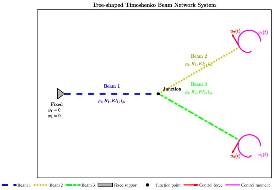
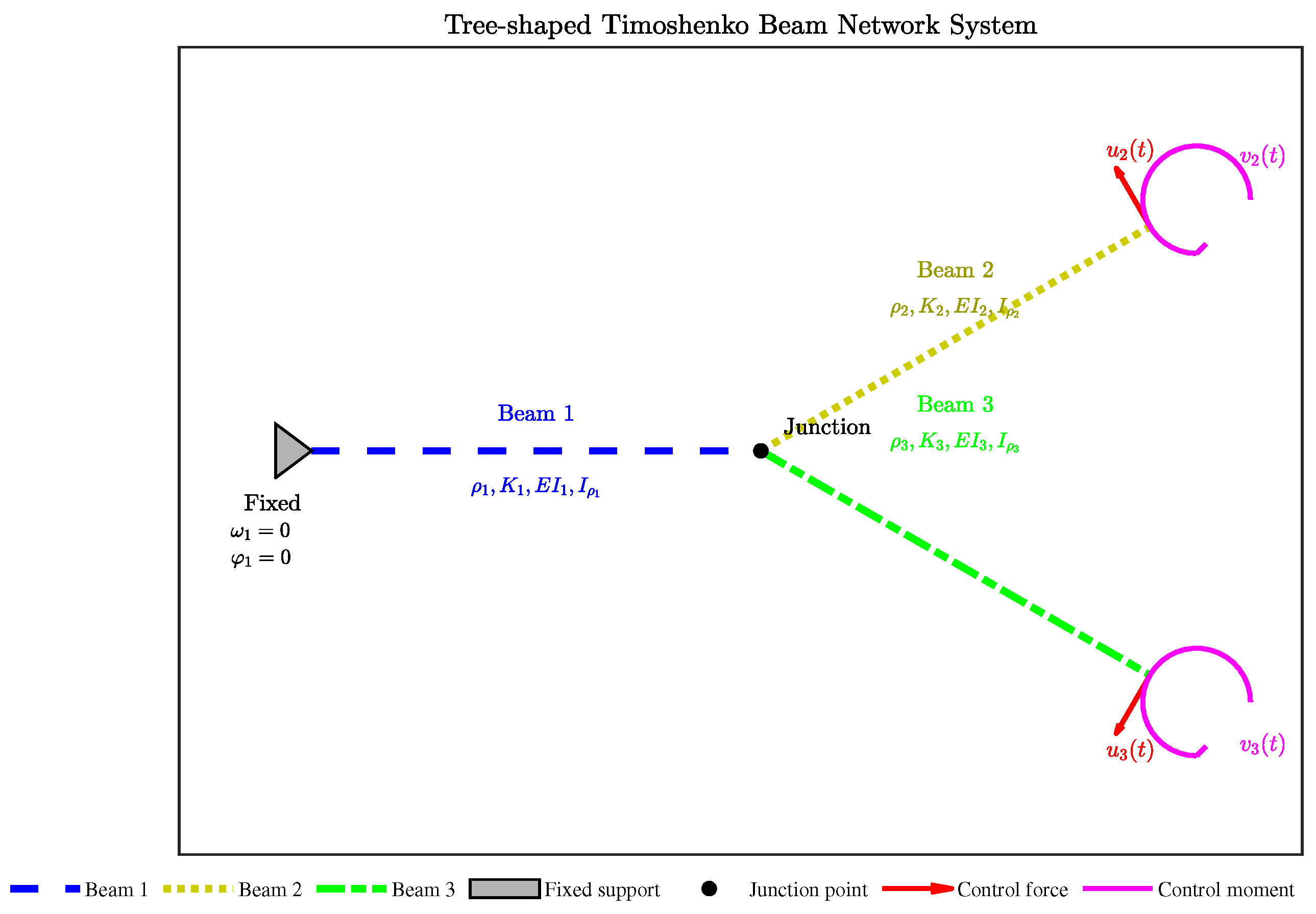
Here, denotes the one-dimensional spatial coordinate, and denotes time. The deflection of the beam from its equilibrium is represented by , while is the rotation angle of the beam at position x. Subscripts such as those in , indicate partial derivatives with respect to time and space, respectively. The physical parameters (mass inertia), (mass density), (bending stiffness), and K (shear stiffness) are all positive constants. Finally, and denote the external force and torque applied at the controlled boundary, respectively.
A simplified schematic of the model is provided in Figure 1:
Figure 1.
Tree-shaped Timoshenko Beam Network System.
3. Exponential Stability of the Timoshenko Beam System
3.1. Closed-Loop System
For Equation (1), we introduce the following auxiliary variables:
where
For each beam , we define the auxiliary variables:
and define the state vector:
Then the standard form of the system (1) is given by the following:
The energy functional of the system (1) is given by the following:
Then, by combining the auxiliary variables, we define the energy functional of the system (1) as follows:
and
where the weight functions are given by
Theorem 1.
The energy functions and are equivalent.
Proof.
Since is a closed interval and the exponential function is continuous and bounded, constants exist:
From the definitions of , we obtain the following identities:
Summing these four equations, the cross-terms cancel, yielding
Substituting and , and using the definition of , we get
Using the uniform upper bound , we obtain
Inserting yields
Let ; then .
Similarly, using , we obtain
Substituting the same integral identity gives
Setting , we have .
Consequently, there exist positive constants such that , which proves the equivalence of and . □
Remark 1.
The exponential form of the weight functions biases the energy functional toward the controlled boundary at (), where the actuators are located. The exponent are determined by the wave speed a and the control gains so as to ensure that the time derivative of satisfies a strict dissipative inequality. The constants M and m serve merely as uniform upper and lower bounds for the weight functions over ; they are technical tools for establishing the equivalence between and and do not affect the control law or the decay rate estimate.
Before proceeding to the stability analysis, we briefly discuss the well-posedness of the closed-loop system within the standard semigroup framework for Timoshenko beam networks [25,26]. Let the state vector be
with , , and define the energy space
equipped with the inner product induced by the energy norm given in (6). The system can be rewritten as the first-order evolution equation
where the operator is defined by
with domain
The domain is dense in . A direct computation using the boundary conditions yields
which shows that is dissipative.
To establish maximal dissipativity, it remains to prove that . For , consider the resolvent equation
Taking the inner product with W in and using the dissipative estimate, we obtain
which implies the a priori bound
To prove that exists on the whole space , we invoke the standard coercivity estimate for the stationary Timoshenko beam network with the prescribed boundary conditions. Indeed, the elliptic system corresponding to can be written componentwise as
with . Eliminating and , we obtain a fourth-order elliptic system for . The transmission conditions at the junction and the boundary feedback conditions ensure that the associated bilinear form is coercive on the appropriate subspace of . Using the Lax–Milgram theorem, this system admits a unique solution for every . Hence is surjective for every , and the resolvent estimate above guarantees boundedness of . Therefore .
Using the Lumer-Phillips theorem [29], generates a -semigroup of contractions on . Consequently, for every initial datum , there exists a unique mild solution ; for , the solution is classical. This provides the required functional setting for the stability analysis that follows.
To stabilize the system, we adopt the control functions as follows:
Accordingly, the closed-loop system corresponding to (1) is given as follows:
where , , , , .
Differentiating with respect to time yields
Here,
Thus,
where
3.2. Exponential Stability of the Closed-Loop System
Theorem 2.
The closed-loop system (11) is exponentially stable with respect to the energy, and its exponential decay rate is at least , where
Proof.
We first consider :
where .
We choose the parameters as follows:
Remark 2.
The choices , , and their rotational analogues, are sufficient conditions adopted for analytical convenience. They ensure that the cross-coupling terms arising from the junction conditions can be absorbed by the dissipative boundary terms via Young’s inequality. The factor 3 corresponds to the three branches meeting at the junction. These selections are not optimal; other choices are possible and would yield different decay rate estimates. Our present choice is made to obtain a transparent explicit expression for the decay rate while preserving the negativity of the Lyapunov derivative.
Substituting the above parameter choices into the expression for gives
where
For convenience, we define
To ensure , we require
which simplifies to
Hence,
We next consider . Applying the transmission conditions yields
For , it is sufficient that
which gives .
Summarizing the analysis of , we obtain
Next, we analyze . Proceeding in a completely analogous way, we obtain
where .
With the following choices
we obtain
where
For simplicity, we define
To ensure , the equivalent condition is
which simplifies to
Then, we have
For , it is sufficient that
which yields .
Hence, for the parameters in , we obtain
Finally, we consider the remaining term .
We define the auxiliary quantities
Using the identities
we can rewrite as
Defining , we obtain
and hence
Using Young’s inequality, for any , we have
With , we have the integral bounds
Substituting into the above estimate yields , where . Similarly, with , we obtain .
Remark 3.
The parameter is chosen as a sufficient condition to absorb the coupling terms via Young’s inequality:
The resulting constants
can be made arbitrarily small by making sufficiently large relative to and .
Therefore .
From the above derivations, we have
where
and the terms satisfy
with
Consequently,
where
Applying Gronwall’s inequality gives
Since is equivalent to the system energy , it follows that
which proves that the closed-loop system is exponentially stable with a decay rate of at least in terms of the original energy .
Combining all the estimates, we finally found that the closed-loop system (11) is exponentially stable with an exponential decay rate of at least , where satisfies
□
To illustrate the practical relevance of the proposed theoretical framework, we consider a lightweight flexible robotic manipulator composed of three interconnected beams arranged in a tree-shaped topology, with a payload mounted at the end effector. This configuration is representative of structural systems found in aerospace engineering and advanced manufacturing. Using realistic material parameters for steel, the derived explicit decay rate in Theorem 2 directly guides the selection of feedback gains (, ).
4. Numerical Simulation
To validate the exponential stability of the proposed system, we perform numerical simulations based on the theoretical analysis presented above. The system is solved numerically using a finite difference method.
The parameters used in the simulations are as follows, as summarized in Table 1.
Table 1.
Key Parameters of Timoshenko Beam System.
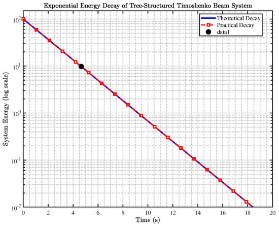
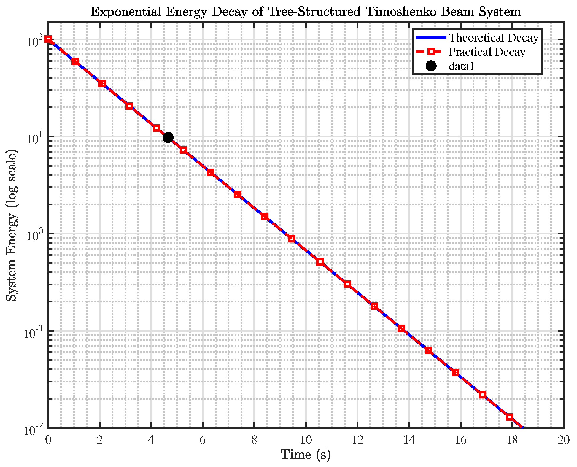
The numerical simulation results are shown in Figure 2.
Figure 2.
Exponential Energy Decay of Tree-Structured Timoshenko Beam System.
Figure 2 shows the decay of the system energy over time in a semi-logarithmic coordinate system. Numerical results indicate that the time required for the system energy to decay to 10% of its initial value is 4.7 s, while the time to decay to 1% is 9.3 s. In the semi-logarithmic plot, the theoretical decay curve is strictly linear, thereby confirming the exponential stability of the system. Furthermore, these simulation results are consistent with the conclusion of Theorem 2 in the theoretical analysis of Section 3, validating the effectiveness and feasibility of the designed boundary velocity feedback control strategy.
Moreover, to quantitatively assess the sharpness of the decay estimate derived in Theorem 2, we extract the observed decay rate from the numerical energy decay curve presented in Figure 2. Applying a least-squares linear regression to over the exponential decay regime yields . This value exceeds the theoretical lower bound established in Theorem 2, confirming that the analytical estimate is valid while being conservative-a feature inherent to Lyapunov-based stability analyses. The comparison validates the theoretical result and quantifies the gap between the worst-case analytical guarantee and the actual numerical performance.
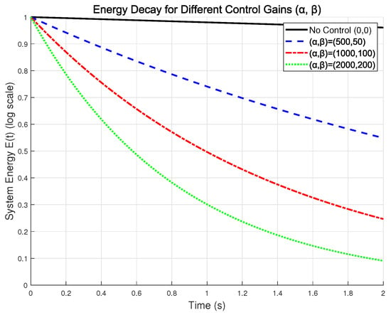
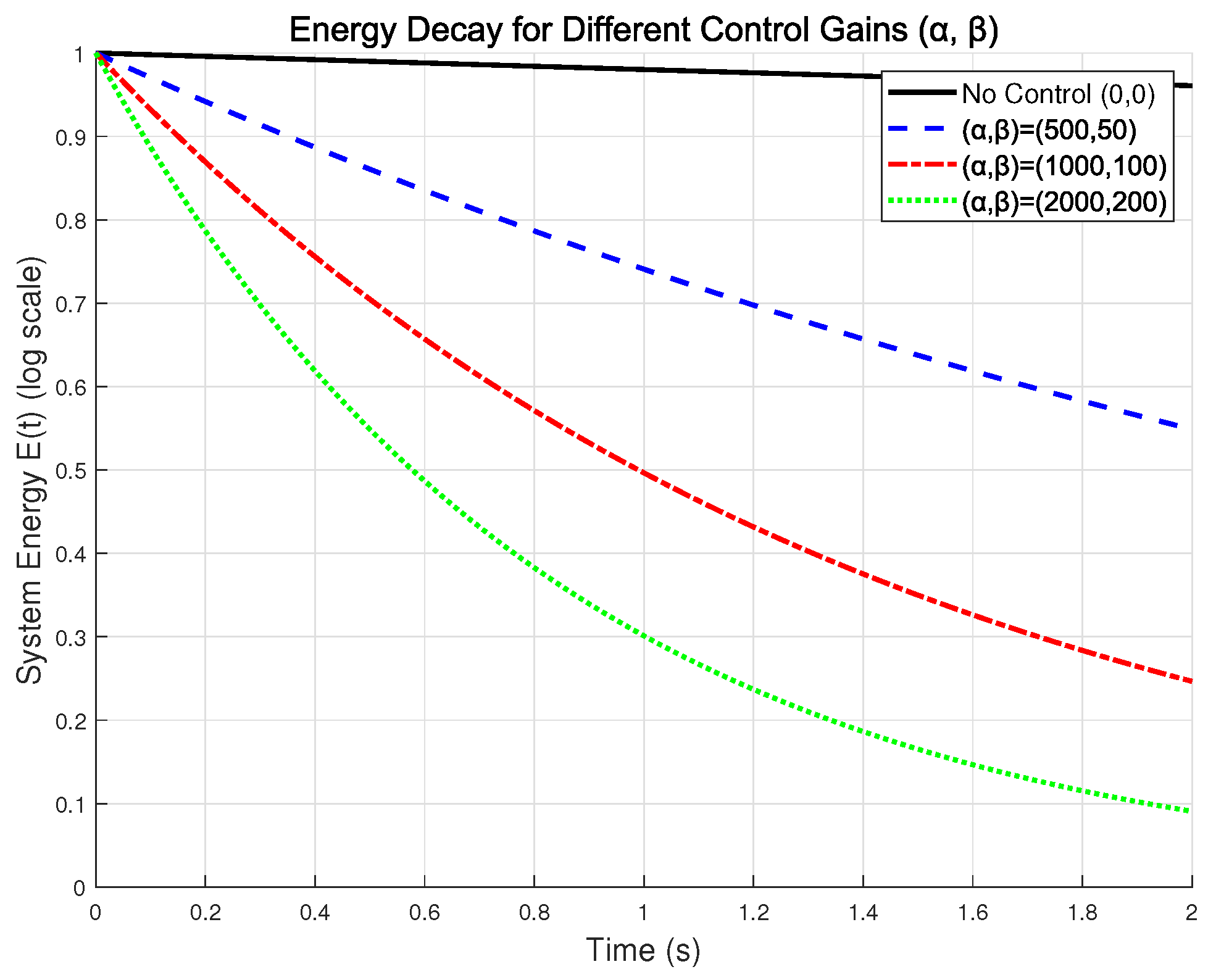
To further explore the influence of control parameters on the decay performance, we conducted a series of numerical experiments with four gain combinations: no control , , , and .
Figure 3 shows the system energy in a semi-logarithmic plot for different control gain combinations. The black solid line corresponds to the uncontrolled case, while the blue dashed, red dash-dotted, and green dotted lines correspond to , , and , respectively. The nearly horizontal black curve indicates that the system is not exponentially stable without control. In contrast, the linear decay observed in the semi-log scale for the controlled cases confirms exponential stability. Moreover, the increasing slopes with larger gains demonstrate the effectiveness of the proposed boundary feedback strategy.
Figure 3.
Energy Decay for Different Control Gains (,).
5. Conclusions
In this paper, we estimate the energy decay rate of the Timoshenko beam system by constructing and employing a weighted energy functional. Specifically, for the case where a concentrated end load is attached to the right end of the beam, we adopt a boundary-velocity feedback control law. We rigorously prove the exponential stability of the system and derive an explicit expression for the decay rate of the weighted energy functional, from which the actual energy decay rate of the system is obtained as .
The appropriate selection of control and structural parameters is crucial for the effectiveness of the proposed method. Based on the explicit decay rate formula in Theorem 2 and the numerical results in Section 4, we provide a preliminary qualitative assessment of parameter sensitivity. The material parameters (, K, , ) influence the decay rate through the wave speeds , , as well as the auxiliary terms and . Among these, the shear stiffness K and bending stiffness have a more pronounced effect than the density or the mass inertia . Meanwhile, increasing the control gains and accelerates dissipation, although excessively large values risk saturating the actuators and exciting high-frequency dynamics.
Author Contributions
Conceptualization, Y.X.; methodology, M.G.; software, Y.X.; validation, Y.X., M.G. and Y.L.; resources, Y.X.; writing—original draft preparation, M.G.; writing—review and editing, Y.X. and Y.L.; supervision, Y.X.; project administration, Y.X.; funding acquisition, Y.X. and Y.L. All authors have read and agreed to the published version of the manuscript.
Funding
This research was funded by National Natural Science Foundation of China (NSFC) grant numbers 12301579, 12301569 and The Research Startup Fund of Civil Aviation University of China grant number G.No.2020KYQD98.
Institutional Review Board Statement
Not applicable.
Informed Consent Statement
Not applicable.
Data Availability Statement
No new data were created or analyzed in this study. Data sharing is not applicable to this article.
Conflicts of Interest
The authors declare no conflicts of interest.
References
- Timoshenko, S.P. On the correction for shear of the differential equation for transverse vibrations of prismatic bars. Lond. Edinb. Dublin Philos. Mag. J. Sci. 1921, 41, 744–746. [Google Scholar] [CrossRef] [Scilit]
- Cowper, G.R. The Shear Coefficient in Timoshenko’s Beam Theory. J. Appl. Mech. 1966, 33, 335–340. [Google Scholar] [CrossRef] [Scilit]
- Han, S.M.; Benaroya, H.; Wei, T. Dynamics of transversely vibrating beams using four engineering theories. J. Sound Vib. 1999, 225, 935–988. [Google Scholar] [CrossRef] [Scilit]
- Arboleda-Monsalve, L.G.; Zapata-Medina, D.G.; Aristizabal-Ochoa, J.D. Timoshenko beam-column with generalized end conditions on elastic foundation: Dynamic-stiffness matrix and load vector. J. Sound Vib. 2008, 310, 1057–1079. [Google Scholar] [CrossRef] [Scilit]
- Calio, I.; Greco, A. Free vibrations of Timoshenko beam-columns on Pasternak foundations. J. Vib. Control 2013, 19, 686–696. [Google Scholar]
- Schnabl, S.; Saje, M.; Turk, G.; Planinc, I. Locking-free two-layer Timoshenko beam element with interlayer slip. Finite Elem. Anal. Des. 2007, 43, 705–714. [Google Scholar] [CrossRef] [Scilit]
- Zougheib, H.; El Arwadi, T.; Madureira, R.L.; Rincon, M.A.; Sayah, T. Exponential stability of a fully discrete energy associated to a thermoviscoelastic Timoshenko system. J. Therm. Stresses 2025, 49, 635–650. [Google Scholar] [CrossRef] [Scilit]
- Rivera, J.E.M.; Racke, R. Global stability for damped Timoshenko systems. Discret. Contin. Dyn. Syst. 2012, 9, 1625–1639. [Google Scholar] [CrossRef] [Scilit]
- Rivera, J.E.M.; Racke, R. Timoshenko systems with indefinite damping. J. Math. Anal. Appl. 2008, 341, 1068–1083. [Google Scholar] [CrossRef] [Scilit]
- Raposo, C.A.; Ferreira, J.; Santos, M.L.; Castro, N.N.O. Exponential stability for the Timoshenko system with two weak dampings. Appl. Math. Lett. 2005, 18, 535–541. [Google Scholar] [CrossRef] [Scilit]
- Shi, D.H.; Feng, D.X. Exponential decay rate of the energy of a Timoshenko beam with locally distributed feedback. ANZIAM J. 2002, 44, 205–220. [Google Scholar] [CrossRef] [Scilit]
- Calsavara, B.M.R.; Tavares, E.G.; Silva, M.J. Exponential stability for a thermo-viscoelastic Timoshenko system with fading memory. J. Math. Anal. Appl. 2022, 512, 126–147. [Google Scholar] [CrossRef] [Scilit]
- Kirane, M.; Said-Houari, B.; Anwar, M.N. Stability result for the Timoshenko system with a time-varying delay term in the internal feedbacks. Commun. Pure Appl. Anal. 2017, 10, 667–686. [Google Scholar] [CrossRef] [Scilit]
- Rivera, J.E.M.; Sare, H.D.F. Stability of Timoshenko systems with past history. J. Math. Anal. Appl. 2008, 339, 482–502. [Google Scholar] [CrossRef] [Scilit]
- Nonato, C.A.; Santos, M.J.D.; Avila, J.A.; Raposo, C.A. A stability and numerical study of the solutions of a Timoshenko system with distributed delay. Math. Nachrichten 2023, 296, 2090–2108. [Google Scholar] [CrossRef] [Scilit]
- Xu, G.Q.; Wang, H.X. Stabilisation of Timoshenko beam system with delay in the boundary control. Int. J. Control 2013, 86, 1165–1178. [Google Scholar] [CrossRef] [Scilit]
- Liu, X.F.; Xu, G.Q. Exponential stabilization for Timoshenko beam with distributed delay in the boundary control. Abstr. Appl. Anal. 2013, 2013, 726794. [Google Scholar] [CrossRef] [Scilit]
- Laribi, I.; Krelifa, A.; Boukabcha, H.; Ouchenane, D.; Boulaaras, S.; Zitouni, S.; Jan, R. Exponential stability and numerical results of a thermoelastic Timoshenko system with diffusion effect, memory and distributed delay terms. Bound. Value Probl. 2024, 2024, 168. [Google Scholar] [CrossRef] [Scilit]
- Chen, W.R. Bending vibration of axially loaded Timoshenko beams with locally distributed kelvin–Voigt damping. J. Sound Vib. 2011, 330, 3040–3056. [Google Scholar] [CrossRef] [Scilit]
- Jiang, J.Q.; Chen, W.Q.; Pao, Y.H. Reverberation-ray analysis of continuous Timoshenko beams subject to moving loads. J. Vib. Control 2012, 18, 744–784. [Google Scholar]
- Wu, D.; Endo, T.; Matsuno, F. Exponential stability of two Timoshenko arms for grasping and manipulating an object. Int. J. Control Autom. Syst. 2020, 19, 1328–1339. [Google Scholar] [CrossRef] [Scilit]
- Mattioni, A.; Wu, Y.; Le Gorrec, Y. Exponential stabilization of a clamped Timoshenko beam with actuation on a tip mass. In Proceedings of the 2021 60th IEEE Conference on Decision and Control (CDC), Austin, TX, USA, 14 December 2021. [Google Scholar]
- Liu, Y.; Chen, X.B.; Mei, Y.F.; Wu, Y.L. Observer-based boundary control for an asymmetric output-constrained flexible robotic manipulator. Sci. China Inf. Sci. 2022, 65, 139203. [Google Scholar]
- Xu, G.Q. Exponential stabilisation of a simple tree-shaped network of Timoshenko beams system. Int. J. Control 2010, 83, 1485–1503. [Google Scholar] [CrossRef] [Scilit]
- Xu, G.Q.; Han, Z.J. Dynamical behavior of networks of non-uniform Timoshenko beams system with boundary time-delay inputs. Netw. Heterog. Media 2012, 6, 297–327. [Google Scholar]
- Macchelli, A.; Melchiorri, C. Control by interconnection of the Timoshenko beam. IFAC Proc. Vol. 2003, 36, 153–158. [Google Scholar] [CrossRef] [Scilit]
- Mishurenko, N.; Semenov, A. Influence of Discretely Introduced Cutouts on the Buckling of Shallow Shells with Double Curvature. J. Appl. Comput. Mech. 2024, 10, 55–63. [Google Scholar]
- Balizadeh, A.M.; Yaghootian, A.; Sedighi, H.M. Elastic Wave Isolation and Highly Directive Wave Propagation in Architected Two-Dimensional Metamaterials: An Accelerated Algebraic Approach. Complex Multiphys. Eng. Syst. 2026, 1, 1–37. [Google Scholar] [CrossRef] [Scilit]
- Glenn, F.; Webb. Semigroups of Linear Operators and Applications to Partial Differential Equations. SIAM Rev. 1985, 27, 309–311. [Google Scholar] [CrossRef] [Scilit]

Disclaimer/Publisher’s Note: The statements, opinions and data contained in all publications are solely those of the individual author(s) and contributor(s) and not of MDPI and/or the editor(s). MDPI and/or the editor(s) disclaim responsibility for any injury to people or property resulting from any ideas, methods, instructions or products referred to in the content. |
© 2026 by the authors. Licensee MDPI, Basel, Switzerland. This article is an open access article distributed under the terms and conditions of the Creative Commons Attribution (CC BY) license.