Geometric Characteristics of Meromorphic Starlike Functions Linked with a Novel Image Domain

Abstract

The present article is mainly concerned with radius problems for a newly defined subclass of meromorphic starlike functions having the punctured open unit disk as its domain. This subclass is introduced by using differential subordination with the generalized tangent function $q_0\left(z\right)=1+\tan \left(\mu z\right)$ as the superordinate function. Sharp radius constants are established for starlikeness and convexity of order $\rho$, and the ${\mathfrak{MS}}_{\tan \mu }^{*}$-radii are determined for several notable subclasses, including Janowski-type classes and classes represented through quotients of meromorphic functions. We further introduce a tangent-order subclass ${\mathfrak{MS}}_{\tan \mu ,\sigma }^{*}$, obtain its representation formula, and derive corresponding starlikeness and convexity radius estimates. Finally, the superordinate tangent function is studied from the viewpoint of conformal mapping theory: its conformality, inverse mapping, boundary parametrization, disk inclusions, and conformal range criterion are established and illustrated graphically.

1. Introduction

Complex analysis is an essential branch of mathematics that has wide-ranging applications in many branches of mathematics. The study of the geometry of analytic functions forms one of the essential divisions of complex analysis known as Geometric Function Theory (G.F.T.). Over the years, considerable attention has been paid to the subclasses of analytic and meromorphic functions whose image domains have geometric representations. Subordination plays an essential role in such investigations, as it provides an effective way to define function classes and analyze their geometric features.

We start with reviewing basic concepts and results of geometric function theory which will be needed in this paper. Suppose $\mathfrak{A}$ is the family of analytic and normalized functions in the unit disk $\mathbb{D}=\{z\in \mathbb{C}:|z|<1\}$ which can be represented as follows:

$$\mathfrak{f}\left(z\right)=z+{\displaystyle \sum _{n=2}^{\infty }}{a}_n{z}^n=z+a_2{z}^2+a_3{z}^3+\cdots .$$

For $n\in \mathbb{N}$, let ${\mathfrak{A}}_n$ be the subfamily comprising of functions of the form:

$$\mathfrak{f}\left(z\right)=z+a_{n+1}{z}^{n+1}+a_{n+2}{z}^{n+2}+\cdots .$$

In particular, ${\mathfrak{A}}_1=\mathfrak{A}$. Suppose that $\mathfrak{f}$ and $\mathfrak{g}$ are analytic in the open unit disk $\mathbb{D}$. Then $\mathfrak{f}$ is said to be subordinate to $\mathfrak{g}$, written as $\mathfrak{f}\prec \mathfrak{g}$, when there is a map $\omega$ that is analytic in $\mathbb{D}$ and $\omega \left(0\right)=0$ such that

$$\mathfrak{f}\left(z\right)=\mathfrak{g}\left(\omega \right(z\left)\right)$$

for each $z\in \mathbb{D}$. Further, the concept of univalent functions is at the core and a cornerstone due to its extensive applicability in function theory. If $\mathfrak{g}$ is univalent in $\mathbb{D}$, then $\mathfrak{f}\prec \mathfrak{g}$ if and only if $\mathfrak{f}\left(0\right)=\mathfrak{g}\left(0\right)$ and $\mathfrak{f}\left(\mathbb{D}\right)\subseteq \mathfrak{g}\left(\mathbb{D}\right)$. Next, let $\mathfrak{M}$ represent the family of meromorphic functions defined on the unit disc $\mathbb{D}$ such that they have a simple pole at $z=0$ and admit the Laurent series expansion

$$\mathfrak{f}\left(z\right)={\displaystyle \frac{1}{z}}+{\displaystyle \sum _{n=0}^{\infty }}{a}_n{z}^n,$$

for all $z\in {\mathbb{D}}^{*}$, where ${\mathbb{D}}^{*}=\mathbb{D}\setminus \left\{0\right\}$. Now for all $n\in \mathbb{N}$, we will consider the subclasses ${\mathfrak{M}}_n$ of functions $\mathfrak{f}$ belonging to $\mathfrak{M}$ such that

$$z\mathfrak{f}\left(z\right)=1+a_n{z}^{n+1}+a_{n+1}{z}^{n+2}+\cdots .$$

Different subclasses of meromorphic functions have been widely studied in geometric function theory. A function $\mathfrak{f}\in \mathfrak{M}$ satisfies the inequality

$$-{\displaystyle \frac{z{\mathfrak{f}}^{\prime }\left(z\right)}{\mathfrak{f}\left(z\right)}}\prec {\displaystyle \frac{1+z}{1-z}},z\in {\mathbb{D}}^{*},$$

then it is said to be meromorphically starlike, and the class of all such functions is represented by ${\mathfrak{MS}}^{*}$. Clunie [1] proved that if $\mathfrak{f}\in {\mathfrak{MS}}^{*}$ then $\left|a_n\right|\le {\displaystyle \frac{2}{n+1}}$. More results have been found for other meromorphic functions by Libera and Robertson [2] and Pommerenke [3]. For further fundamental work in this direction, see [4,5,6,7,8]. Let $\phi$ be a given analytic function, and let ${\mathfrak{MS}}^{*}\left(\phi \right)$ denote the set of meromorphic starlike functions which satisfy

$$-{\displaystyle \frac{z{\mathfrak{f}}^{\prime }\left(z\right)}{\mathfrak{f}\left(z\right)}}\prec \phi \left(z\right).$$

In this case, the symbol used in brackets refers to the choice of $\phi$ made to construct the appropriate subclass.

$$\begin{array}{ccc}\hfill {\mathfrak{MS}}_L^{*}& =& {\mathfrak{MS}}^{*}\left(\sqrt{1+z}\right),\hfill \\ \hfill {\mathfrak{MS}}_{RL}^{*}& =& {\mathfrak{MS}}^{*}\left(\sqrt{2}-\left(\sqrt{2}-1\right)\sqrt{{\displaystyle \frac{1-z}{1+2\left(\sqrt{2}-1\right)z}}}\right),\hfill \\ \hfill {\mathfrak{MS}}_C^{*}& =& {\mathfrak{MS}}^{*}\left(1+{\displaystyle \frac{4z}{3}}+{\displaystyle \frac{2z^2}{3}}\right).\hfill \end{array}$$

Similarly, selecting

$${\varphi }_{\rho }\left(z\right)={\displaystyle \frac{1+(1-2\rho )z}{1-z}},0\le \rho <1,$$

as the function in the classes ${\mathfrak{MS}}^{*}\left(\varphi \right)$ and $\mathfrak{MC}\left(\varphi \right)$, we get the class of meromorphic functions of order $\rho$ and they are

$${\mathfrak{MS}}^{*}\left(\rho \right)={\mathfrak{MS}}^{*}\left({\varphi }_{\rho }\right),\mathfrak{MC}\left(\rho \right)=\mathfrak{MC}\left({\varphi }_{\rho }\right).$$

In particular, ${\mathfrak{MS}}^{*}\left(0\right)={\mathfrak{MS}}^{*}$ and $\mathfrak{MC}\left(0\right)=\mathfrak{MC},$ where $\mathfrak{MC}$ represents the family enclosing meromorphic convex functions. Furthermore, the subclasses ${\mathfrak{MS}}^{*}\left[L,M\right]$ and $\mathfrak{MC}\left[L,M\right]$ respectively, denote meromorphic, Janowski starlike, and Janowski convex functions and are deduced from the above-mentioned classes by choosing $\varphi \left(z\right)={\displaystyle \frac{1+Lz}{1+Mz}}$ with $-1\le M<L\le 1$. These notions were expanded and thoroughly investigated in [9,10,11,12]. The class ${\mathfrak{MH}}_{\alpha }\left(\varphi \right)$, ($0\le \alpha \le 1$) of $\alpha$-convex univalent meromorphic functions encompasses both these classes and was introduced by Ali and Ravichandran [13]. In fact the class ${\mathfrak{MH}}_{\alpha }\left(\varphi \right)$ generalizes ${\mathfrak{MS}}^{*}\left(\varphi \right)$ and $\mathfrak{MC}\left(\varphi \right)$. That is

$${\mathfrak{MS}}^{*}\left(\varphi \right)={\mathfrak{MH}}_0\left(\varphi \right)\mathrm{and}\mathfrak{MC}\left(\varphi \right)={\mathfrak{MH}}_1\left(\varphi \right).$$

A similar attempt is taken in [14] by introducing a unified class ${\mathfrak{MG}}_{b,n}\left(\varphi \right)$, where $b\in \mathbb{C}\setminus \left\{0\right\}$ and $n\in \mathbb{N}$, of meromorphic functions, connected with ${\mathfrak{MS}}^{*}\left(\varphi \right)$ and $\mathfrak{MC}\left(\varphi \right)$ as:

$${\mathfrak{MG}}_{2,0}\left(\varphi \right)={\mathfrak{MS}}^{*}\left(\varphi \right)\mathrm{and}{\mathfrak{MG}}_{1,1}\left(\varphi \right)=\mathfrak{MC}\left(\varphi \right).$$

However, the function $1+\tan z$ is not positive in the real part in the unit disk. In order to solve this problem, we use the parameter $\mu$ such that $0\le \mu \le \pi /4$, and we define the generalized tangent function as follows:

$$q_0\left(z\right)=1+\tan \left(\mu z\right).$$

This function plays the role of the superordinate function for our newly defined meromorphic starlike function class.

Now, we introduce the class of meromorphic starlike functions as:

$${\mathfrak{MS}}_{\tan \mu }^{*}=\left\{\mathfrak{f}\in \mathfrak{M}:-{\displaystyle \frac{z{\mathfrak{f}}^{\prime }\left(z\right)}{\mathfrak{f}\left(z\right)}}\prec 1+\tan \left(\mu z\right):=q_0\left(z\right),\mathrm{for}0\le \mu \le {\displaystyle \frac{\pi }{4}},z\in {\mathbb{D}}^{*}\right\},$$

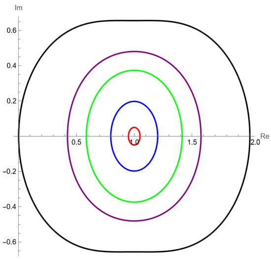
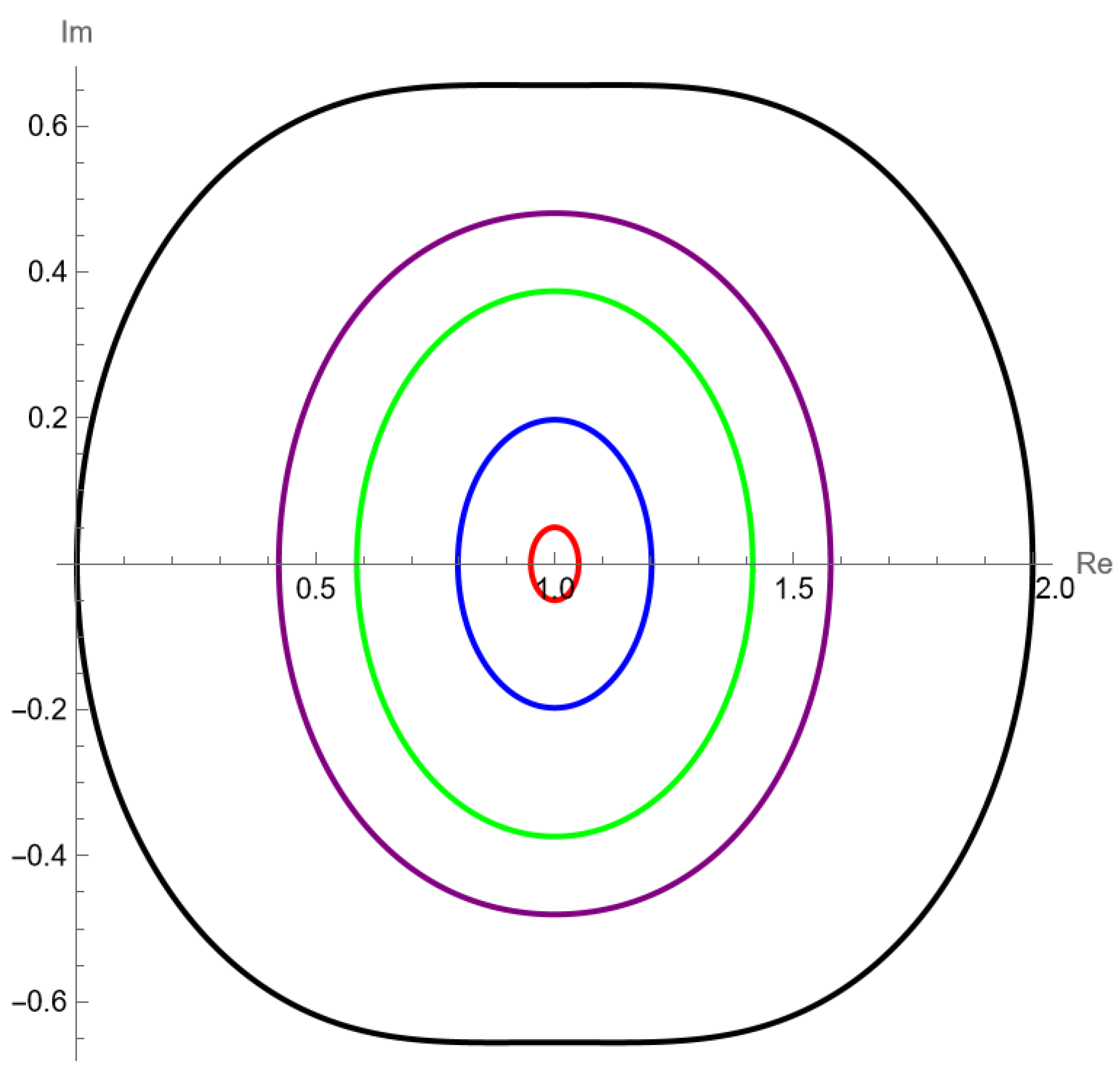
The behavior of the generalized tangent function $q_0\left(z\right)=1+\tan \left(\mu z\right)$ for several values of $\mu$ is illustrated in Figure 1.

Figure 1. Plots of the function $q_0\left(z\right)=1+\tan \left(\mu z\right)$ for several values of $\mu$ in the interval $0\le \mu \le {\displaystyle \frac{\pi }{4}}$. The curves correspond to $\mu =0.05$ (red), $\mu =0.2$ (blue), $\mu ={\displaystyle \frac{\pi }{8}}$ (green), $\mu ={\displaystyle \frac{\pi }{6}}$ (purple), and $\mu ={\displaystyle \frac{\pi }{4}}$ (black).

One can observe that a function $\mathfrak{f}\in {\mathfrak{MS}}_{\tan \mu }^{*}$ has a representation

$$\mathfrak{f}\left(z\right)={\displaystyle \frac{1}{z}}\exp {\int }_0^z{\displaystyle \frac{1-q\left(t\right)}{t}}dt,$$

if $q\left(z\right)\prec q_0\left(z\right)=1+\tan \left(\mu z\right)$ for $z\in \mathbb{D}$ and vice versa. Observe that

$$\begin{array}{ccc}{q}_1\left(z\right)=1+{\displaystyle \frac{\mu }{4}}z,& q_2\left(z\right)={\displaystyle \frac{4+\left(2\mu +1\right)z}{4+z}},& \mathrm{and}{q}_3\left(z\right)={\displaystyle \frac{5+\left(1+3\mu \right)z}{5+z}}\end{array}$$

along with the univalent function $q_0\left(z\right)=1+\tan \left(\mu z\right)$ in $\mathbb{D}$ are such that $q_i\left(0\right)=q_0\left(0\right)=1$, $q_i\left(\mathbb{D}\right)\subseteq q_0\left(\mathbb{D}\right)$; therefore, $q_i\prec q_0$ for $i=1,2,3$. Hence, their respective functions ${\mathfrak{f}}_i^{\prime }s$ for $i=1,2,3$, given by

$$\begin{array}{ccc}\hfill {\mathfrak{f}}_1\left(z\right)& =& {\displaystyle \frac{1}{z}}\exp \left(-{\displaystyle \frac{\mu }{4}}z\right),\hfill \\ \hfill {\mathfrak{f}}_2\left(z\right)& =& {\displaystyle \frac{1}{z}}{\left({\displaystyle \frac{4}{z+4}}\right)}^{2\mu },\hfill \\ \hfill {\mathfrak{f}}_3\left(z\right)& =& {\displaystyle \frac{1}{z}}{\left({\displaystyle \frac{5}{z+5}}\right)}^{3\mu }.\hfill \end{array}$$

The central aim and focus of this study is to identify the radius r regarding starlikeness and convexity of ${\mathfrak{MS}}_{\tan \mu }^{*}$. Additionally, we extend our study to calculate the ${\mathfrak{MS}}_{\tan \mu }^{*}$-radius for several intriguing classes, including that of Janowski starlike functions. Furthermore, we discuss the ${\mathfrak{MS}}_{\tan \mu }^{*}$-radius about classes whose functions are the ratio of two meromorphic functions.

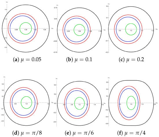
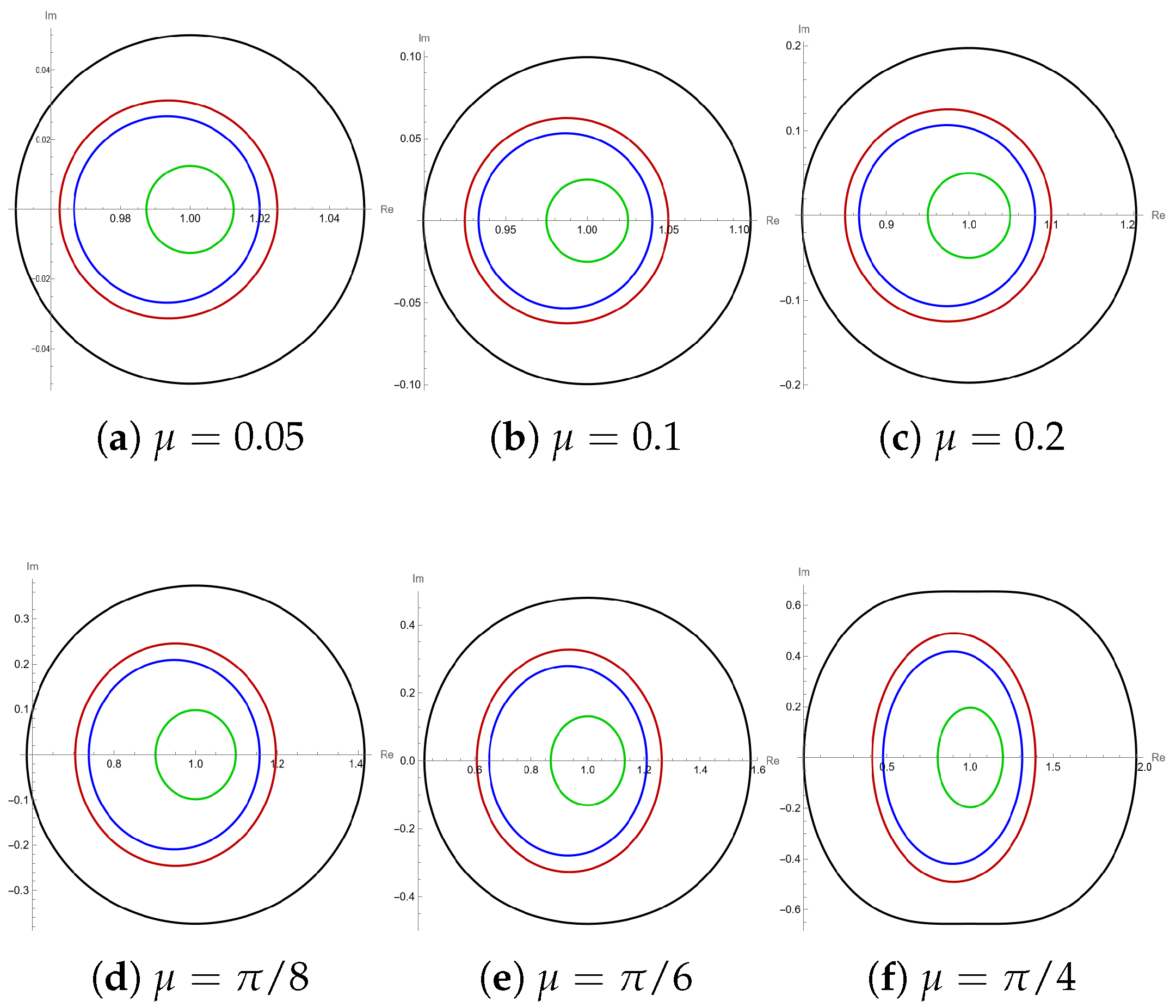
The corresponding mappings for several values of $\mu$ are displayed in Figure 2.

Figure 2. Representative images of the mappings of the unit disk under the functions $\mathfrak{f}\left[\mu \right]\left(z\right)$ (black), $q_1\left(z\right)$ (green), $q_2\left(z\right)$ (blue), and $q_3\left(z\right)$ (red) for various values of the parameter $\mu$. Each subfigure illustrates the behavior for a specific $\mu$, showing the deformation of the unit disk under these transformations.

Problems related to the radius have been extensively studied in geometric function theory. Kwon et al. [15] addressed several radius problems concerning a certain family of holomorphic functions. In the context of meromorphic functions, Cho et al. [16] obtained criteria for meromorphic strongly starlike functions. Further research has also been conducted by Ali et al. [17], Tayyah and Atshan [18], Sharma et al. [19], Cho et al. [20] and Tayyah et al. [21]. Their notable contributions inspired and influenced our current investigation.

2. Radius of Starlikeness and Convexity

Here, we explore the highlighted radii in the class ${\mathfrak{MS}}_{\tan \mu }^{*}.$ The ${\mathfrak{MS}}^{*}\left(\rho \right)$-radius (or ${\mathfrak{MK}}^{*}\left(\rho \right)$-radius) for ${\mathfrak{MS}}_{\tan \mu }^{*}$ to obtain the largest $r_0$ with the property that every function in ${\mathfrak{MS}}_{\tan \mu }^{*}$ is also in ${\mathfrak{MS}}^{*}\left(\rho \right)$ (or ${\mathfrak{MK}}^{*}\left(\rho \right)$) on each open disc $\left|z\right|<r$ for all $r<r_0$.

Theorem 1.

Let $\mu \in \left(0,\pi /4\right]$ and $1-\tan \left(\mu \right)\le \rho <1$. Then, the ${\mathfrak{MS}}^{*}\left(\rho \right)$-radius for the class ${\mathfrak{MS}}_{\tan \mu }^{*}$ is $r_0={\displaystyle \frac{1}{\mu }}{\tan }^{-1}\left(1-\rho \right).$

Proof. 

If $\mathfrak{f}\in {\mathfrak{MS}}_{\tan \mu }^{*}$ then a Schwarz function $\omega \left(z\right)$ exists, implying

$$-{\displaystyle \frac{z{\mathfrak{f}}^{\prime }\left(z\right)}{\mathfrak{f}\left(z\right)}}=1+\tan \left(\mu \omega \left(z\right)\right).$$

Taking $\omega \left(z\right)=R{e}^{i\vartheta }$, $R\le \left|z\right|=r$, $-\pi \le \vartheta \le \pi ,$ we consider

$$\begin{array}{c}{D}_{\vartheta }={\cos }^2\left(\mu R\cos \vartheta \right)+{\sinh }^2\left(\mu R\sin \vartheta \right),\\ {\left|\tan \left(\mu R{e}^{i\vartheta }\right)\right|}^2={\left({\displaystyle \frac{\sin \left(\mu R\cos \vartheta \right)\cos \left(\mu R\cos \vartheta \right)}{D_{\vartheta }}}\right)}^2+{\left({\displaystyle \frac{\sinh \left(\mu R\sin \vartheta \right)\cosh \left(\mu R\sin \vartheta \right)}{D_{\vartheta }}}\right)}^2:=h\left(\vartheta \right).\end{array}$$

Since $\mathfrak{h}\left(-\vartheta \right)=\mathfrak{h}\left(\vartheta \right)$, so we take $0\le \vartheta \le \pi$ instead of $-\pi \le \vartheta \le \pi$. The equation $h^{\prime }\left(\vartheta \right)=0$ has the roots $\vartheta =0,$ ${\displaystyle \frac{\pi }{2}},$ $\pi$. Moreover, $\mathfrak{h}\left(0\right)={\tan }^2\mu R=\mathfrak{h}\left(\pi \right),$ $\mathfrak{h}\left({\displaystyle \frac{\pi }{2}}\right)={\tanh }^2\mu R$ and since ${\tan }^2\mu R-{\tanh }^2\mu R\ge 0,$ so

$$\max \left\{\mathfrak{h}\left(0\right),\mathfrak{h}\left(\pi /2\right),\mathfrak{h}\left(\pi \right)\right\}={\tan }^2\mu R\le {\tan }^2\mu r.$$

(1)

Therefore,

$$\mathfrak{Re}\left(-{\displaystyle \frac{z{\mathfrak{f}}^{\prime }\left(z\right)}{\mathfrak{f}\left(z\right)}}\right)\ge 1-\left|\tan \left(\mu \omega \left(z\right)\right)\right|\ge 1-\tan \mu r\ge \rho ,$$

subject to $1-\tan \mu r-\rho \ge 0$. The required radius for ${\mathfrak{MS}}_{\tan \mu }^{*}$ is then the root $r_0\in \left(0,1\right]$, of $1-\tan \mu r-\rho =0$. □

Theorem 2.

For the class ${\mathfrak{MS}}_{\tan \mu }^{*}$, the $\mathfrak{MK}\left(\rho \right)$-radius is $\min \{r_1,r_2\}$, where $r_1>0$ is the smallest root of

$$\left(1-\tan \mu r\right)\left(1-\tan \mu r-\rho \right)(1-r^2)-\mu r{\sec }^2\mu r=0$$

and $r_2={\mu }^{-1}{\tan }^{-1}(1-\rho )$.

Proof. 

For $\mathfrak{f}\in {\mathfrak{MS}}_{\tan \mu }^{*}$, as before, we have a Schwarz function $\omega \left(z\right)$, for which

$$-{\displaystyle \frac{z{\mathfrak{f}}^{\prime }\left(z\right)}{\mathfrak{f}\left(z\right)}}=1+\tan \left(\mu \omega \left(z\right)\right).$$

Logarithmic differentiation gives

$$-1-{\displaystyle \frac{z{\mathfrak{f}}^{″}\left(z\right)}{{\mathfrak{f}}^{\prime }\left(z\right)}}=1+\tan \left(\mu \omega \left(z\right)\right)-{\displaystyle \frac{z{\omega }^{\prime }\left(z\right)\mu {\sec }^2\left(\mu \omega \left(z\right)\right)}{1+\tan \left(\mu \omega \left(z\right)\right)}}.$$

(2)

From (2),

$$\mathfrak{Re}\left(-1-{\displaystyle \frac{z{\mathfrak{f}}^{″}\left(z\right)}{{\mathfrak{f}}^{\prime }\left(z\right)}}\right)\ge 1-\left|\tan \left(\mu \omega \left(z\right)\right)\right|-{\displaystyle \frac{\mu \left|z{\omega }^{\prime }\left(z\right)\right|\left|{\sec }^2\left(\mu \omega \left(z\right)\right)\right|}{1-\left|\tan \left(\mu \omega \left(z\right)\right)\right|}}.$$

(3)

Now consider

$$\begin{array}{cc}\hfill {\left|\sec \left(\mu R{e}^{i\vartheta }\right)\right|}^2& ={\displaystyle \frac{1}{{\left|\cos \left(\mu R{e}^{i\vartheta }\right)\right|}^2}}\hfill \\ \hfill & ={\displaystyle \frac{1}{{\cos }^2\left(\mu R\cos \vartheta \right){\cosh }^2\left(\mu R\sin \vartheta \right)+{\sin }^2\left(\mu R\cos \vartheta \right){\sinh }^2\left(\mu R\sin \vartheta \right)}}\hfill \\ \hfill & ={\displaystyle \frac{1}{{\cos }^2\left(\mu R\cos \vartheta \right)+{\sinh }^2\left(\mu R\sin \vartheta \right)}}:=h_1\left(\vartheta \right),\hfill \end{array}$$

Since ${\mathfrak{h}}_1\left(-\vartheta \right)={\mathfrak{h}}_1\left(\vartheta \right)$, we take $0\le \vartheta \le \pi$ instead of $-\pi \le \vartheta \le \pi$. Then ${\mathfrak{h}}_1^{\prime }\left(\vartheta \right)=0$ has the roots $\vartheta =0,$ $\pi /2,$ $\pi$. Moreover, we observe that ${\mathfrak{h}}_1\left(0\right)={\sec }^2\mu R={\mathfrak{h}}_1\left(\pi \right),$ and ${\mathfrak{h}}_1\left(\pi /2\right)={sech}^2\mu R$ with ${\sec }^2\mu R-{sech}^2\mu R\ge 0,$ thus

$$\max \left\{h_1\left(0\right),h_1\left(\pi /2\right),h_1\left(\pi \right)\right\}={\sec }^2\mu R\le {\sec }^2\mu r.$$

(4)

It follows from (1) and (4) that

$$\left|\tan \left(\mu \omega \left(z\right)\right)\right|\le \tan \mu r\mathrm{and}\left|\sec \left(\mu \omega \left(z\right)\right)\right|\le \sec \mu r.$$

(5)

Now, using the famous Schwarz inequality

$$\left|{\omega }^{\prime }\left(z\right)\right|\le {\displaystyle \frac{1-{\left|\omega \left(z\right)\right|}^2}{1-{\left|z\right|}^2}}\le {\displaystyle \frac{1-R^2}{1-{\left|z\right|}^2}}\le {\displaystyle \frac{1}{1-{\left|z\right|}^2}},$$

while (5) in (3) yields

$$\mathfrak{Re}\left(-1-{\displaystyle \frac{z{\mathfrak{f}}^{″}\left(z\right)}{{\mathfrak{f}}^{\prime }\left(z\right)}}\right)\ge 1-\tan \mu r-{\displaystyle \frac{\mu r{\sec }^2\mu r}{\left(1-r^2\right)\left(1-\tan \mu r\right)}}\ge \rho ,$$

provided that

$$1-\tan \mu r-{\displaystyle \frac{\mu r{\sec }^2\mu r}{\left(1-r^2\right)\left(1-\tan \mu r\right)}}-\rho \ge 0.$$

(6)

For $0\le \mu \le \pi /4$ and $0\le r<1$, we have $1-\tan \mu r>0.$ Therefore, from (6), we obtain

$$\left(1-\tan \mu r\right)\left(1-\tan \mu r-\rho \right)(1-r^2)-\mu r{\sec }^2\mu r\ge 0,$$

subject to the condition that $1-\tan \mu r-\rho >0$, that is $\tan \mu r<1-\rho .$ Hence the proof is accomplished. □

As for $\rho =0$ the inequality $\tan \mu r<1-\rho$ is true for all $r\in (0,1);$ thus we observe the following corollary:

Corollary 1.

The $\mathfrak{MK}$-radius $r_0$ for ${\mathfrak{MS}}_{\tan \mu }^{*}$ is the smallest positive number satisfying

$${\left(1-\tan \mu r\right)}^2(1-r^2)-\mu r{\sec }^2\mu r=0.$$

3. Radius Problems

Here in this section, we establish the third Lemma and then extensively use it in the subsequent discussion about ${\mathfrak{MS}}_{\tan \mu }^{*}$-radii for different eminent subfamilies of meromorphic starlike functions. Here, we need to examine few outcomes associated with the class ${\mathfrak{P}}_n\left(L,M\right)$ defined by:

$${\mathfrak{P}}_n\left(L,M\right)=\left\{\mathfrak{p}\left(z\right)=1+{\mathfrak{p}}_n{z}^n+{\mathfrak{p}}_{n+1}{z}^{n+1}+\cdots :\mathfrak{p}\left(z\right)\prec {\displaystyle \frac{1+Lz}{1+Mz}},-1\le M<L\le 1\right\}.$$

To be more specific, we get

$${\mathfrak{P}}_n\left(\rho \right):={\mathfrak{P}}_n\left[1-2\rho ,-1\right]\mathrm{and}{\mathfrak{P}}_n:={\mathfrak{P}}_n\left(0\right).$$

Lemma 1

([22], Lemma 2). For $\mathfrak{p}\in {\mathfrak{P}}_n\left(\rho \right),$ and $\left|z\right|=r$:

$$\left|{\displaystyle \frac{z{\mathfrak{p}}^{\prime }\left(z\right)}{\mathfrak{p}\left(z\right)}}\right|\le {\displaystyle \frac{2\left(1-\rho \right)n{r}^n}{\left(1-r^n\right)\left(1+\left(1-2\rho \right)r^n\right)}}.$$

Lemma 2

([23], Lemma 2.1). If $\mathfrak{p}\in {\mathfrak{P}}_n\left(L,M\right),$ and $\left|z\right|=r$, then

$$\left|\mathfrak{p}\left(z\right)-{\displaystyle \frac{1-LM{r}^{2n}}{1-M^2{r}^{2n}}}\right|\le {\displaystyle \frac{\left(L-M\right)r^n}{1-M^2{r}^{2n}}}.$$

Especially, if $\mathfrak{p}\in {\mathfrak{P}}_n\left(\rho \right),$ then

$$\left|\mathfrak{p}\left(z\right)-{\displaystyle \frac{\left(1+\left(1-2\rho \right)r^{2n}\right)}{1-r^{2n}}}\right|\le {\displaystyle \frac{2\left(1-\rho \right)r^n}{1-r^{2n}}}.$$

For each $\mathfrak{f}\in \mathfrak{M}$, if $\mathfrak{p}\left(z\right)=-{\displaystyle \frac{z{\mathfrak{f}}^{\prime }\left(z\right)}{\mathfrak{f}\left(z\right)}},$ then ${\mathfrak{P}}_n\left(L,M\right)$ turns into ${\mathfrak{MS}}_n^{*}\left(L,M\right)$ and it further implies ${\mathfrak{MS}}_n^{*}\left(\rho \right)={\mathfrak{MS}}_n^{*}\left[1-2\rho ,-1\right].$ Moreover,

$${\mathfrak{MS}}_{\tan ,n}^{*}={\mathfrak{M}}_n\cap {\mathfrak{MS}}_{\tan \mu }^{*},{\mathfrak{MS}}_n^{*}\left(\rho \right)={\mathfrak{M}}_n\cap {\mathfrak{MS}}^{*}\left(\rho \right),{\mathfrak{MS}}_{L,n}^{*}={\mathfrak{M}}_n\cap {\mathfrak{MS}}_L^{*}.$$

Ali et al. [17] defined the class ${\mathfrak{S}}_n=\left\{\mathfrak{f}\in \mathfrak{A}:{\displaystyle \frac{\mathfrak{f}\left(z\right)}{z}}\in {\mathfrak{P}}_n\right\}$ and

$$\mathfrak{C}{\mathfrak{S}}_n=\left\{\mathfrak{f}\in \mathfrak{A}:{\displaystyle \frac{\mathfrak{f}\left(z\right)}{\mathfrak{g}\left(z\right)}}\mathrm{with}\mathfrak{g}\in {\mathfrak{S}}_n^{*}\left(\rho \right)\right\}$$

Now, we define analogous classes for meromorphic functions as:

$${\mathfrak{MS}}_n=\left\{\mathfrak{f}\in \mathfrak{M}:z\mathfrak{f}\left(z\right)\in {\mathfrak{P}}_n\right\}$$

and

$${\mathfrak{MCS}}_n\left(\rho \right)=\left\{\mathfrak{f}\in \mathfrak{M}:{\displaystyle \frac{\mathfrak{f}\left(z\right)}{\mathfrak{g}\left(z\right)}}\in {\mathfrak{P}}_n\mathrm{for}\mathrm{some}\mathfrak{g}\in {\mathfrak{MS}}_n^{*}\left(\rho \right)\right\}.$$

We now establish the following lemma and will extensively use it in the subsequent radii results.

Lemma 3.

If $1-\tan \mu \le a\le 1+\tan \mu ,$ and $r_a=\tan \mu +\left|a-1\right|,$ then

$$\left\{\omega \in \mathbb{C}:\left|\omega -1\right|<\tanh \mu \right\}\subset {\omega }_{\tan \mu }\subset \left\{\omega \in \mathbb{C}:\left|\omega -a\right|<r_a\right\},$$

where,

$${\omega }_{\tan \mu }=\left\{\omega \in \mathbb{C}:\omega =1+\tan \left(\mu z\right),0\le \mu \le \pi /4\mathrm{and}z\in \mathbb{D}\right\}.$$

Proof. 

Let $\omega \in {\omega }_{\tan \mu }$. Then

$$\omega =1+\tan \left(\mu z\right),z=R{e}^{i\vartheta },0\le R<1.$$

For $0\le \mu \le \pi /4$, the estimate for the tangent function used in (1) gives

$${\left|\tan \left(\mu z\right)\right|}^2={\left|\tan \left(\mu R{e}^{i\vartheta }\right)\right|}^2\le {\tan }^2\left(\mu R\right)<{\tan }^2\mu .$$

Thus $\left|\tan \left(\mu z\right)\right|<\tan \mu$. Hence, for every real number a with $1-\tan \mu \le a\le 1+\tan \mu$, we have

$$\left|\omega -a\right|=\left|1-a+\tan \left(\mu z\right)\right|\le |a-1|+\left|\tan \left(\mu z\right)\right|<|a-1|+\tan \mu =r_a.$$

Therefore,

$${\omega }_{\tan \mu }\subset \left\{\omega \in \mathbb{C}:|\omega -a|<r_a\right\}.$$

Next, for a boundary point $1+\tan \left(\mu e^{i\vartheta }\right)$ of ${\omega }_{\tan \mu }$, the distance from the point 1 is $\left|\tan \right(\mu e^{i\vartheta }\left)\right|$. The minimum of this boundary distance is attained at $\vartheta =\pi /2$ and is equal to $\tanh \mu$. Therefore,

$$\left\{\omega \in \mathbb{C}:\left|\omega -1\right|<\tanh \mu \right\}\subset {\omega }_{\tan \mu }.$$

□

Theorem 3.

The best ${\mathfrak{MS}}_{\tan ,n}^{*}$-radius for ${\mathfrak{MS}}_n$ is

$$R_{{\mathfrak{MS}}_{\tan ,n}^{*}}\left({\mathfrak{MS}}_n\right)={\left({\displaystyle \frac{\tanh \mu }{\sqrt{n^2+{\tanh }^2\mu }+n}}\right)}^{1/n}.$$

(7)

Proof. 

Let $\mathfrak{f}\in {\mathfrak{MS}}_n$ and $\mathfrak{h}\left(z\right)=z\mathfrak{f}\left(z\right)$. As a result $\mathfrak{h}\in {\mathfrak{P}}_n$ and

$$-{\displaystyle \frac{z{\mathfrak{f}}^{\prime }\left(z\right)}{\mathfrak{f}\left(z\right)}}-1=-{\displaystyle \frac{z{\mathfrak{h}}^{\prime }\left(z\right)}{\mathfrak{h}\left(z\right)}}.$$

Utilizing Lemma 1 with $\rho =0$, we obtain

$$\left|{\displaystyle \frac{z{\mathfrak{f}}^{\prime }\left(z\right)}{\mathfrak{f}\left(z\right)}}+1\right|=\left|{\displaystyle \frac{z{\mathfrak{h}}^{\prime }\left(z\right)}{\mathfrak{h}\left(z\right)}}\right|\le {\displaystyle \frac{2n{r}^n}{1-r^{2n}}}.$$

By Lemma 3, the inclusion $-{\displaystyle \frac{z{\mathfrak{f}}^{\prime }\left(z\right)}{\mathfrak{f}\left(z\right)}}$ in ${\omega }_{\tan \mu }$ holds whenever

$${\displaystyle \frac{2n{r}^n}{1-r^{2n}}}\le \tanh \mu ,$$

equivalently

$$r^{2n}\tanh \mu +2n{r}^n-\tanh \mu \le 0.$$

Hence, the ${\mathfrak{MS}}_{\tan ,n}^{*}$-radius to ${\mathfrak{MS}}_n$ is the smallest positive solution of $r^{2n}\tanh \mu +2n{r}^n-\tanh \mu =0$, given in (7). For the function ${\mathfrak{f}}_0\left(z\right)={\displaystyle \frac{1+z^n}{z\left(1-z^n\right)}},$ it is straightforward to have $\mathfrak{Re}\left(z\mathfrak{f}\left(z\right)\right)\ge 0$ in $\mathbb{D},$ so, ${\mathfrak{f}}_0\left(z\right)\in {\mathfrak{MS}}_n$, and $-{\displaystyle \frac{z{\mathfrak{f}}_0^{\prime }\left(z\right)}{{\mathfrak{f}}_0\left(z\right)}}=1-{\displaystyle \frac{2n{z}^n}{1-z^{2n}}}.$ Thus, at a boundary point satisfying $z^n=-R_{{\mathfrak{MS}}_{\tan ,n}^{*}}{\left({\mathfrak{MS}}_n\right)}^n$, we obtain

$$-{\displaystyle \frac{z{\mathfrak{f}}_0^{\prime }\left(z\right)}{{\mathfrak{f}}_0\left(z\right)}}-1={\displaystyle \frac{2n{R}_{{\mathfrak{MS}}_{\tan ,n}^{*}}{\left({\mathfrak{MS}}_n\right)}^n}{1-R_{{\mathfrak{MS}}_{\tan ,n}^{*}}{\left({\mathfrak{MS}}_n\right)}^{2n}}}=\tanh \mu .$$

□

Theorem 4.

The ${\mathfrak{MS}}_{\tan ,n}^{*}$-radius to ${\mathfrak{MCS}}_n\left(\rho \right)$ is

$$R_{{\mathfrak{MS}}_{\tan ,n}^{*}}\left({\mathfrak{MCS}}_n\left(\rho \right)\right)={\left({\displaystyle \frac{\tanh \mu }{\sqrt{{\left(1+n-\rho \right)}^2+\left[2\left(1-\rho \right)+\tanh \left(\mu \right)\right]\tanh \left(\mu \right)}+\left(1+n-\rho \right)}}\right)}^{1/n}$$

and is the best one.

Proof. 

Let $\mathfrak{f}\in {\mathfrak{MCS}}_n\left(\rho \right),$ and $\mathfrak{h}\left(z\right)={\displaystyle \frac{\mathfrak{f}\left(z\right)}{\mathfrak{g}\left(z\right)}}$ with $\mathfrak{g}\in {\mathfrak{MS}}_n^{*}\left(\rho \right).$ Then, we have

$$-{\displaystyle \frac{z{\mathfrak{f}}^{\prime }\left(z\right)}{\mathfrak{f}\left(z\right)}}=-{\displaystyle \frac{z{\mathfrak{g}}^{\prime }\left(z\right)}{\mathfrak{g}\left(z\right)}}-{\displaystyle \frac{z{\mathfrak{h}}^{\prime }\left(z\right)}{\mathfrak{h}\left(z\right)}}.$$

Practicing Lemmas 1 and 2, we have

$$\left|-{\displaystyle \frac{z{\mathfrak{f}}^{\prime }\left(z\right)}{\mathfrak{f}\left(z\right)}}-{\displaystyle \frac{1+\left(1-2\rho \right)r^{2n}}{1-r^{2n}}}\right|\le {\displaystyle \frac{2\left(1+n-\rho \right)r^n}{1-r^{2n}}}.$$

As $\left[1+\left(1-2\rho \right)r^{2n}\right]/(1-r^{2n})\ge 1$ due to Lemmas 2 and 3. We reach the conclusion that $\mathfrak{f}\in {\mathfrak{MS}}_{\tan ,n}^{*}$ if the below condition holds

$${\displaystyle \frac{1+\left(1-2\rho \right)r^{2n}}{1-r^{2n}}}+{\displaystyle \frac{2\left(1+n-\rho \right)r^n}{1-r^{2n}}}\le 1+\tanh \mu .$$

This further implies that

$$r\le {\left({\displaystyle \frac{\tanh \mu }{\sqrt{{(1+n-\rho )}^2+{\tanh }^2\mu +2(1-\rho )\tanh \mu }+(n+1-\rho )}}\right)}^{{\displaystyle \frac{1}{n}}}=r_1,$$

Hence $R_{{\mathfrak{MS}}_{\tan ,n}^{*}}\left({\mathfrak{MCS}}_n\left(\rho \right)\right)=r_1.$ Now consider the functions

$${\mathfrak{f}}_0\left(z\right)={\displaystyle \frac{{\left(1-z^n\right)}^{\left(n+2-2\rho \right)/n}}{z\left(1+z^n\right)}},{\mathfrak{g}}_0\left(z\right)={\displaystyle \frac{{\left(1-z^n\right)}^{2\left(1-\rho \right)/n}}{z}}.$$

(8)

Then,

$${\displaystyle \frac{{\mathfrak{f}}_0\left(z\right)}{{\mathfrak{g}}_0\left(z\right)}}={\displaystyle \frac{\left(1-z^n\right)}{\left(1+z^n\right)}}$$

and

$$-{\displaystyle \frac{z{\mathfrak{g}}_0^{\prime }\left(z\right)}{{\mathfrak{g}}_0\left(z\right)}}={\displaystyle \frac{1+\left(1-2\rho \right)z^n}{1-z^n}}.$$

It’s easy to observe that $\mathfrak{Re}\left({\mathfrak{f}}_0\left(z\right)/{\mathfrak{g}}_0\left(z\right)\right)>0$ and $\mathfrak{Re}\left(-{\displaystyle \frac{z{\mathfrak{g}}_0^{\prime }\left(z\right)}{{\mathfrak{g}}_0\left(z\right)}}\right)>\rho .$ Hence ${\mathfrak{f}}_0\in {\mathfrak{MCS}}_n\left(\rho \right)$ then the function ${\mathfrak{f}}_0$ defined in (8) at $z=R_{{\mathfrak{MS}}_{\tan ,n}^{*}}\left({\mathfrak{MCS}}_n\left(\rho \right)\right)$ satisfies

$$-{\displaystyle \frac{z{\mathfrak{f}}_0^{\prime }\left(z\right)}{{\mathfrak{f}}_0\left(z\right)}}={\displaystyle \frac{1+\left(1-2\rho \right)z^{2n}+2\left(1+n-\rho \right)z^n}{1-z^{2n}}}=1+\tanh \mu ,$$

and so is maximal. □

Theorem 5.

The ${\mathfrak{MS}}_{\tan ,n}^{*}$-radius in favor of the class ${\mathfrak{MS}}_n^{*}\left[L,M\right]$ equals

$$R_{{\mathfrak{MS}}_{\tan ,n}^{*}}\left({\mathfrak{MS}}_n^{*}\left[L,M\right]\right)=\left\{\begin{array}{c}\min \left\{1,r_1\right\}:-1\le M\le 0<L\le 1;\hfill \\ \min \left\{1,r_2\right\}:0<M<L\le 1\hfill \end{array}\right.$$

where

$$r_1={\left({\displaystyle \frac{2\tanh \mu }{\left(L-M\right)+\sqrt{{\left(L-M\right)}^2+4\left[M^2\left(1+\tanh \mu \right)-LM\right]\tanh \mu }}}\right)}^{1/n}$$

and

$$r_2={\left({\displaystyle \frac{2\tanh \mu }{\sqrt{{\left(L-M\right)}^2+4\left(M^2\tanh \mu +LM-M^2\right)\tanh \mu }+\left(L-M\right)}}\right)}^{1/n}.$$

Proof. 

Let $\mathfrak{f}\in {\mathfrak{MS}}_n^{*}\left[L,M\right]$. Thus, due to Lemma 2

$$\left|-{\displaystyle \frac{z{\mathfrak{f}}^{\prime }\left(z\right)}{\mathfrak{f}\left(z\right)}}-b\right|\le {\displaystyle \frac{\left(L-M\right)r^n}{1-M^2{r}^{2n}}}.$$

(9)

where at $\left|z\right|=r$, the disk’s center is

$$b={\displaystyle \frac{1-LM{r}^{2n}}{1-M^2{r}^{2n}}}.$$

For $M<0$, we have $b>1.$ Thus by Lemma 3, $\mathfrak{f}\in {\mathfrak{MS}}_{\tan ,n}^{*}$ if

$$\begin{array}{c}\hfill {\displaystyle \frac{\left(L-M\right)r^n}{1-M^2{r}^{2n}}}\le 1+\tanh \mu -{\displaystyle \frac{1-LM{r}^{2n}}{1-M^2{r}^{2n}}},\end{array}$$

further simplification gives

$$r\le {\left({\displaystyle \frac{2\tanh \mu }{\left(L-M\right)+\sqrt{{\left(L-M\right)}^2+4\left[M^2\left(1+\tanh \mu \right)-LM\right]\tanh \mu }}}\right)}^{1/n}=r_1.$$

Moreover, if $M=0$ then $b=1$ and hence from inequality (9)

$$\left|-{\displaystyle \frac{z{\mathfrak{f}}^{\prime }\left(z\right)}{\mathfrak{f}\left(z\right)}}-1\right|\le L{r}^n.$$

Again by Lemma 3, $\mathfrak{f}\in {\mathfrak{MS}}_{\tan ,n}^{*},$ if $L{r}^n\le \tanh \mu$, that is if $r\le {\left(\tanh \mu /L\right)}^{1/n}$ but this is the same as $r_1$ for $M=0.$

Now for $0<M<L\le 1,$ it is simple to prove $b<1$ due to Lemma 3.3 and inequality (9); we have

$${\displaystyle \frac{\left(L-M\right)r^n}{1-M^2{r}^{2n}}}\le {\displaystyle \frac{1-LM{r}^{2n}}{1-M^2{r}^{2n}}}-(1-\tanh \mu ),$$

or,

$${\displaystyle \frac{\left(L-M\right)r^n-1+LM{r}^{2n}}{1-M^2{r}^{2n}}}\le \tanh \mu -1.$$

A manageable calculation yields

$$r\le {\left({\displaystyle \frac{2\tanh \mu }{\left(L-M\right)+\sqrt{{\left(L-M\right)}^2+4\left[M^2\left(\tanh \mu -1\right)+LM\right]\tanh \mu }}}\right)}^{1/n}=r_2.$$

□

Theorem 6.

Let $\mathfrak{f}\in {\mathfrak{MS}}_n^{*}\left[L,M\right]$, where $-1<M<L\le 1$, subject to the conditions

$$(L-M)(1+M)\le \left(1-M^2\right)\tanh \mu \mathit{and}1-LM\le 1-M^2,$$

(10)

or,

$$(L-M)(1-M)\le \left(1-M^2\right)\tanh \mu \mathit{and}1-M^2\le 1-LM.$$

(11)

Then $\mathfrak{f}\in {\mathfrak{MS}}_{\tan ,n}^{*}$, that is ${\mathfrak{MS}}_n^{*}\left[L,M\right]\subset {\mathfrak{MS}}_{\tan ,n}^{*}$.

Proof. 

Let $\mathfrak{f}\in {\mathfrak{MS}}_n^{*}\left[L,M\right]$. From Lemma 2, we have

$$\left|-{\displaystyle \frac{z{\mathfrak{f}}^{\prime }\left(z\right)}{\mathfrak{f}\left(z\right)}}-{\displaystyle \frac{1-LM}{1-M^2}}\right|\le {\displaystyle \frac{L-M}{1-M^2}}.$$

Also, because of Lemma 3, we observe that $\mathfrak{f}\in {\mathfrak{MS}}_{\tan ,n}^{*}$ if

$${\displaystyle \frac{L-M}{1-M^2}}\le {\displaystyle \frac{1-LM}{1-M^2}}-\left(1-\tanh \mu \right)\mathrm{and}{\displaystyle \frac{1-LM}{1-M^2}}\le 1$$

or,

$${\displaystyle \frac{L-M}{1-M^2}}\le 1+\tanh \mu -{\displaystyle \frac{1-LM}{1-M^2}}\mathrm{and}1\le {\displaystyle \frac{1-LM}{1-M^2}},$$

which, after some simple calculations, yields conditions (10) and (11) respectively. □

Theorem 7.

The ${\mathfrak{MS}}_{\tan \mu }^{*}$-radii for the classes ${\mathfrak{MS}}_L^{*}$, ${\mathfrak{MS}}_{RL}^{*}$ and ${\mathfrak{MS}}_C^{*}$ are, respectively:

$$\begin{array}{ccc}\hfill R_{{\mathfrak{MS}}_{\tan \mu }^{*}}\left({\mathfrak{MS}}_L^{*}\right)& =& \tanh \mu \left(2-\tanh \mu \right),\hfill \\ \hfill R_{{\mathfrak{MS}}_{\tan \mu }^{*}}\left({\mathfrak{MS}}_{RL}^{*}\right)& =& {\displaystyle \frac{\tanh \mu \left(2\left(\sqrt{2}-1\right)+\tanh \mu \right)}{{\left(\sqrt{2}-1\right)}^2+2\left(\sqrt{2}-1\right){\left(\sqrt{2}-1+\tanh \mu \right)}^2}},\hfill \end{array}$$

and

$$R_{{\mathfrak{MS}}_{\tan \mu }^{*}}\left({\mathfrak{MS}}_C^{*}\right)={\displaystyle \frac{\sqrt{2\left(2+3\tanh \mu \right)}-2}{2}}.$$

All these radii cannot be improved.

Proof. 

If $\mathfrak{f}\in {\mathfrak{MS}}_L^{*}$ then $-{\displaystyle \frac{z{\mathfrak{f}}^{\prime }\left(z\right)}{\mathfrak{f}\left(z\right)}}\prec \sqrt{1+z}$. Therefore, if $\left|z\right|=r$,

$$\left|-{\displaystyle \frac{z{\mathfrak{f}}^{\prime }\left(z\right)}{\mathfrak{f}\left(z\right)}}-1\right|\le 1-\sqrt{1-r}$$

and because of Lemma 3, $\mathfrak{f}\in {\mathfrak{MS}}_{\tan ,n}^{*}$ if

$$1-\sqrt{1-r}\le \tanh \mu ,$$

that is,

$$r\le \tanh \mu \left(2-\tanh \mu \right)=R_{{\mathfrak{MS}}_{\tan \mu }^{*}}\left({\mathfrak{MS}}_L^{*}\right).$$

For the sharpness, we have

$${\mathfrak{f}}_0\left(z\right)={\displaystyle \frac{{\left(1+\sqrt{1+z}\right)}^2}{4z\exp \left\{2\left(\sqrt{1+z}-1\right)\right\}}}.$$

Clearly $-{\displaystyle \frac{z{\mathfrak{f}}_0^{\prime }\left(z\right)}{{\mathfrak{f}}_0\left(z\right)}}=\sqrt{1+z},$ so $\mathfrak{f}\in {\mathfrak{MS}}_L^{*}$. Letting $z=-R_{{\mathfrak{MS}}_{\tan \mu }^{*}}\left({\mathfrak{MS}}_L^{*}\right)$ implies $-{\displaystyle \frac{z{\mathfrak{f}}_0^{\prime }\left(z\right)}{{\mathfrak{f}}_0\left(z\right)}}-1=-\tanh \mu$. Hence, the radius is sharp. Next, on behalf of $\mathfrak{f}\in {\mathfrak{MS}}_{RL}^{*}$

$$-{\displaystyle \frac{z{\mathfrak{f}}^{\prime }\left(z\right)}{\mathfrak{f}\left(z\right)}}\prec \sqrt{2}-\left(\sqrt{2}-1\right)\sqrt{{\displaystyle \frac{1-z}{1+2\left(\sqrt{2}-1\right)z}}}.$$

Now, if $\left|z\right|=r,$ then

$$\left|-{\displaystyle \frac{z{\mathfrak{f}}^{\prime }\left(z\right)}{\mathfrak{f}\left(z\right)}}-1\right|\le 1-\sqrt{2}+\left(\sqrt{2}-1\right)\sqrt{{\displaystyle \frac{1+r}{1-2\left(\sqrt{2}-1\right)r}}}$$

and again by employing Lemma 3, $\mathfrak{f}\in {\mathfrak{MS}}_{\tan ,n}^{*}$ if

$$1-\sqrt{2}+\left(\sqrt{2}-1\right)\sqrt{{\displaystyle \frac{1+r}{1-2\left(\sqrt{2}-1\right)r}}}\le \tanh \mu .$$

Further simplification gives

$$r\le {\displaystyle \frac{\tanh \mu \left(2\left(\sqrt{2}-1\right)+\tanh \mu \right)}{{\left(\sqrt{2}-1\right)}^2+2\left(\sqrt{2}-1\right){\left(\sqrt{2}-1+\tanh \mu \right)}^2}}=R_{{\mathfrak{MS}}_{\tan \mu }^{*}}\left({\mathfrak{MS}}_{RL}^{*}\right).$$

where

$$q_{RL}\left(z\right)=\sqrt{2}-\left(\sqrt{2}-1\right)\sqrt{{\displaystyle \frac{1-z}{1+2\left(\sqrt{2}-1\right)z}}}.$$

Sharpness follows for

$${\mathfrak{f}}_1\left(z\right)={\displaystyle \frac{1}{z}}\exp \left({\int }_0^z{\displaystyle \frac{1-q_{RL}\left(t\right)}{t}}dt\right),$$

where the integral is taken along any path in $\mathbb{D}$ from 0 to z. It is easy to see that

$$-{\displaystyle \frac{z{\mathfrak{f}}_1^{\prime }\left(z\right)}{{\mathfrak{f}}_1\left(z\right)}}=q_{RL}\left(z\right)=\sqrt{2}-\left(\sqrt{2}-1\right)\sqrt{{\displaystyle \frac{1-z}{1+2\left(\sqrt{2}-1\right)z}}}.$$

Hence, by taking $z=-R_{{\mathfrak{MS}}_{\tan \mu }^{*}}\left({\mathfrak{MS}}_{RL}^{*}\right)$, we obtain

$$-{\displaystyle \frac{z{\mathfrak{f}}_1^{\prime }\left(z\right)}{{\mathfrak{f}}_1\left(z\right)}}-1=-\tanh \mu ,$$

which shows the sharpness of the result. Finally, let $\mathfrak{f}\in {\mathfrak{MS}}_C^{*}$ and $\left|z\right|=r$. Then

$$-{\displaystyle \frac{z{\mathfrak{f}}^{\prime }\left(z\right)}{\mathfrak{f}\left(z\right)}}\prec 1+{\displaystyle \frac{4z}{3}}+{\displaystyle \frac{2z^2}{3}}.$$

Therefore

$$\left|-{\displaystyle \frac{z{\mathfrak{f}}^{\prime }\left(z\right)}{\mathfrak{f}\left(z\right)}}-1\right|\le {\displaystyle \frac{4r}{3}}+{\displaystyle \frac{2r^2}{3}},$$

from Lemma 3, we conclude that $\mathfrak{f}\in {\mathfrak{MS}}_{\tan ,n}^{*}$ if

$${\displaystyle \frac{4r}{3}}+{\displaystyle \frac{2r^2}{3}}\le \tanh \mu ,$$

which further gives

$$r\le {\displaystyle \frac{\sqrt{2\left(2+3\tanh \mu \right)}-2}{2}}=R_{{\mathfrak{MS}}_{\tan \mu }^{*}}\left({\mathfrak{MS}}_C^{*}\right).$$

We consider the function below to prove the sharpness

$${\mathfrak{f}}_2\left(z\right)={\displaystyle \frac{1}{z\exp \left(\frac{4z+z^2}{3}\right)}}.$$

Since

$$-{\displaystyle \frac{z{\mathfrak{f}}_2^{\prime }\left(z\right)}{{\mathfrak{f}}_2\left(z\right)}}=1+{\displaystyle \frac{4z}{3}}+{\displaystyle \frac{2z^2}{3}}.$$

Therefore ${\mathfrak{f}}_2\in {\mathfrak{MS}}_C^{*},$ and at $z=R_{{\mathfrak{MS}}_{\tan \mu }^{*}}\left({\mathfrak{MS}}_C^{*}\right)$, we get $-z{\mathfrak{f}}_2^{\prime }\left(z\right)/{\mathfrak{f}}_2\left(z\right)-1=\tanh \mu$, which proves that the result is sharp. □

4. Classes of Functions Associated with the Ratio Functions

In this section, for a fixed $n\in \mathbb{N}$, we introduce the classes associated with ratios of meromorphic functions as follows.

$$\begin{array}{ccc}\hfill {\mathfrak{F}}_1& =& \left\{\mathfrak{f}\in {\mathfrak{M}}_n:\mathfrak{Re}\left({\displaystyle \frac{\mathfrak{f}\left(z\right)}{\mathfrak{g}\left(z\right)}}\right)>0\mathrm{and}\mathfrak{Re}\left(z\mathfrak{g}\left(z\right)\right)>0,\mathfrak{g}\left(z\right)\in {\mathfrak{M}}_n\right\},\hfill \\ \hfill {\mathfrak{F}}_2& =& \left\{\mathfrak{f}\in {\mathfrak{M}}_n:\mathfrak{Re}\left({\displaystyle \frac{\mathfrak{f}\left(z\right)}{\mathfrak{g}\left(z\right)}}\right)>0\mathrm{and}\mathfrak{Re}\left(z\mathfrak{g}\left(z\right)\right)>{\displaystyle \frac{1}{2}},\mathfrak{g}\left(z\right)\in {\mathfrak{M}}_n\right\},\hfill \\ \hfill {\mathfrak{F}}_3& =& \left\{\mathfrak{f}\in {\mathfrak{M}}_n:\left|{\displaystyle \frac{\mathfrak{f}\left(z\right)}{\mathfrak{g}\left(z\right)}}-1\right|<1\mathrm{and}\mathfrak{Re}\left(z\mathfrak{g}\left(z\right)\right)>0,\mathfrak{g}\left(z\right)\in {\mathfrak{M}}_n\right\},\hfill \end{array}$$

$$\begin{array}{c}\hfill {\mathfrak{F}}_4=\left\{\mathfrak{f}\in {\mathfrak{M}}_n:\left|{\displaystyle \frac{\mathfrak{f}\left(z\right)}{\mathfrak{g}\left(z\right)}}-1\right|<1\mathrm{and}\mathfrak{g}\in {\mathfrak{M}}_n\mathrm{is}\mathrm{convex}\right\}.\end{array}$$

Theorem 8.

The ${\mathfrak{MS}}_{\tan \mu }^{*}$-radii for the class ${\mathfrak{F}}_1,{\mathfrak{F}}_2,{\mathfrak{F}}_3$, and ${\mathfrak{F}}_4$ respectively are

$$\begin{array}{ccc}\hfill R_{{\mathfrak{MS}}_{\tan \mu }^{*}}\left({\mathfrak{F}}_1\right)& =& {\left(\sqrt{4n^2{\coth }^2\left(\mu \right)+1}-2n\coth \left(\mu \right)\right)}^{1/n},\hfill \\ \hfill R_{{\mathfrak{MS}}_{\tan \mu }^{*}}\left({\mathfrak{F}}_2\right)& =& {\left({\displaystyle \frac{\sqrt{9n^2+4\tanh \mu \left(n+\tanh \mu \right)}-3n}{2\left(n+\tanh \mu \right)}}\right)}^{1/n},\hfill \\ \hfill R_{{\mathfrak{MS}}_{\tan \mu }^{*}}\left({\mathfrak{F}}_3\right)& =& {\left({\displaystyle \frac{\sqrt{9n^2+4\tanh \mu \left(n+\tanh \mu \right)}-3n}{2\left(n+\tanh \mu \right)}}\right)}^{1/n},\hfill \\ \hfill R_{{\mathfrak{MS}}_{\tan \mu }^{*}}\left({\mathfrak{F}}_4\right)& =& {\left({\displaystyle \frac{\tanh \mu }{n+1+\tanh \mu }}\right)}^{{\displaystyle \frac{1}{n}}}.\hfill \end{array}$$

Proof. 

Let $\mathfrak{f}\in {\mathfrak{F}}_1$, then some $\mathfrak{g}\in \mathfrak{M}$ with $\mathfrak{Re}\left(\mathfrak{f}\left(z\right)/\mathfrak{g}\left(z\right)\right)>0$ and $\mathfrak{Re}\left(z\mathfrak{g}\left(z\right)\right)>0$ exists. Now, if $\mathfrak{p}$ and $\mathfrak{h}$ are defined as $\mathfrak{p}\left(z\right)=z\mathfrak{g}\left(z\right)$ and $\mathfrak{h}\left(z\right)=\mathfrak{f}\left(z\right)/\mathfrak{g}\left(z\right),$ then $\mathfrak{p},\mathfrak{h}\in {\mathfrak{P}}_n$. Thus, $\mathfrak{f}\left(z\right)=\mathfrak{p}\left(z\right)\mathfrak{h}\left(z\right)/z$. Hence, by Lemma 1

$$\left|-{\displaystyle \frac{z{\mathfrak{f}}^{\prime }\left(z\right)}{\mathfrak{f}\left(z\right)}}-1\right|\le {\displaystyle \frac{4n{r}^n}{1-r^{2n}}}.$$

Due to Lemma 3, $\mathfrak{f}\in {\mathfrak{MS}}_{\tan ,n}^{*}$ if

$${\displaystyle \frac{4n{r}^n}{1-r^{2n}}}\le \tanh \mu ,$$

which on further calculation gives

$$r\le {\left(\sqrt{4n^2{\coth }^2\left(\mu \right)+1}-2n\coth \left(\mu \right)\right)}^{1/n}=R_{{\mathfrak{MS}}_{\tan \mu }^{*}}\left({\mathfrak{F}}_1\right).$$

For the sharpness, consider

$${\mathfrak{f}}_0\left(z\right)={\displaystyle \frac{1}{z}}{\left({\displaystyle \frac{1-z^n}{1+z^n}}\right)}^2,{\mathfrak{g}}_0\left(z\right)={\displaystyle \frac{1}{z}}\left({\displaystyle \frac{1-z^n}{1+z^n}}\right).$$

Obviously $\mathfrak{Re}\left({\mathfrak{f}}_0\left(z\right)/{\mathfrak{g}}_0\left(z\right)\right)>0$ and $\mathfrak{Re}\left(z{\mathfrak{g}}_0\left(z\right)\right)>0$; hence ${\mathfrak{f}}_0\in {\mathfrak{F}}_1$.

Now, by taking a boundary point satisfying $z^n=R_{{\mathfrak{MS}}_{\tan \mu }^{*}}{\left({\mathfrak{F}}_1\right)}^n,$ we obtain

$$-{\displaystyle \frac{z{\mathfrak{f}}_0^{\prime }\left(z\right)}{{\mathfrak{f}}_0\left(z\right)}}-1={\displaystyle \frac{4n{z}^n}{1-z^{2n}}}=\tanh \left(\mu \right),$$

which implies that the radius is sharp.

If $\mathfrak{f}\in {\mathfrak{F}}_2$ then by definition we have $\mathfrak{g}\in \mathfrak{M}$ with $\mathfrak{Re}\left(\mathfrak{f}\left(z\right)/\mathfrak{g}\left(z\right)\right)$ being positive and $\mathfrak{Re}\left(z\mathfrak{g}\left(z\right)\right)>1/2$. Now, let $\mathfrak{h}\left(z\right)$ and $\mathfrak{p}\left(z\right)$ be as $\mathfrak{p}\left(z\right)=z\mathfrak{g}\left(z\right)$, $\mathfrak{h}\left(z\right)=\mathfrak{f}\left(z\right)/\mathfrak{g}\left(z\right).$ Then, it is straightforward that $\mathfrak{h}\in {\mathfrak{P}}_n$ while $\mathfrak{p}\in {\mathfrak{P}}_n\left(1/2\right)$. As before, $\mathfrak{f}\left(z\right)=\mathfrak{p}\left(z\right)\mathfrak{h}\left(z\right)/z$. From Lemma 1

$$\left|-{\displaystyle \frac{z{\mathfrak{f}}^{\prime }\left(z\right)}{\mathfrak{f}\left(z\right)}}-1\right|\le {\displaystyle \frac{3n{r}^n+n{r}^{2n}}{1-r^{2n}}}$$

and in view of Lemma 3, $\mathfrak{f}\in {\mathfrak{MS}}_{\tan ,n}^{*},$ if

$${\displaystyle \frac{3n{r}^n+n{r}^{2n}}{1-r^{2n}}}\le \tanh \mu ,$$

that is,

$$r\le {\left({\displaystyle \frac{\sqrt{9n^2+4\tanh \mu \left(n+\tanh \mu \right)}-3n}{2\left(n+\tanh \mu \right)}}\right)}^{1/n}=R_{{\mathfrak{MS}}_{\tan \mu }^{*}}\left({\mathfrak{F}}_2\right).$$

For the sharpness, consider

$${\mathfrak{f}}_0\left(z\right)={\displaystyle \frac{\left(1+z^n\right)}{z{\left(1-z^n\right)}^2}},{\mathfrak{g}}_0\left(z\right)={\displaystyle \frac{1}{z\left(1-z^n\right)}}.$$

Since $\mathfrak{Re}\left({\mathfrak{f}}_0\left(z\right)/{\mathfrak{g}}_0\left(z\right)\right)>0$ with $\mathfrak{Re}\left(z{\mathfrak{g}}_0\left(z\right)\right)>1/2$, thus ${\mathfrak{f}}_0\in {\mathfrak{F}}_2$. By taking a boundary point satisfying $z^n=R_{{\mathfrak{MS}}_{\tan \mu }^{*}}{\left({\mathfrak{F}}_2\right)}^n$, we obtain

$$-{\displaystyle \frac{z{\mathfrak{f}}_0^{\prime }\left(z\right)}{{\mathfrak{f}}_0\left(z\right)}}-1=-{\displaystyle \frac{3n{R}^n+n{R}^{2n}}{1-R^{2n}}}=-\tanh \mu ,$$

which implies the sharpness.

Let $\mathfrak{f}\in {\mathfrak{F}}_3$. Then there must exist some $\mathfrak{g}\in \mathfrak{M}$ with the properties that $\left|\mathfrak{f}\left(z\right)/\mathfrak{g}\left(z\right)-1\right|<1$ with $\mathfrak{Re}\left(z\mathfrak{g}\left(z\right)\right)$ being positive. Therefore, if $\mathfrak{p}\left(z\right)=z\mathfrak{g}\left(z\right)$ and $\mathfrak{h}\left(z\right)=\mathfrak{g}\left(z\right)/\mathfrak{f}\left(z\right)$ then $p\in {\mathfrak{P}}_n$ and $\left|1/\mathfrak{h}\left(z\right)-1\right|<1$ iff $\mathfrak{Re}\left(\mathfrak{h}\left(z\right)\right)>{\displaystyle \frac{1}{2}}$, i.e., $\mathfrak{h}\in {\mathfrak{P}}_n\left(1/2\right).$ Further as

$$\mathfrak{h}\left(z\right)={\displaystyle \frac{\mathfrak{p}\left(z\right)}{z\mathfrak{f}\left(z\right)}},$$

so logarithmic differentiation and the use of triangle inequality yields

$$\begin{array}{ccc}\hfill \left|-{\displaystyle \frac{z{\mathfrak{f}}^{\prime }\left(z\right)}{\mathfrak{f}\left(z\right)}}-1\right|& \le & \left|{\displaystyle \frac{z{\mathfrak{h}}^{\prime }\left(z\right)}{\mathfrak{h}\left(z\right)}}\right|+\left|{\displaystyle \frac{z{\mathfrak{p}}^{\prime }\left(z\right)}{\mathfrak{p}\left(z\right)}}\right|,\hfill \end{array}$$

and the application of Lemma 1 for $\rho =0$ and then for $\rho =1/2$, respectively, produces the result

$$\begin{array}{ccc}\hfill \left|-{\displaystyle \frac{z{\mathfrak{f}}^{\prime }\left(z\right)}{\mathfrak{f}\left(z\right)}}-1\right|& \le & {\displaystyle \frac{n{r}^n}{1-r^n}}+{\displaystyle \frac{2n{r}^n}{1-r^{2n}}}.\hfill \end{array}$$

Thus, because of Lemma 3 $\mathfrak{f}\in {\mathfrak{MS}}_{\tan ,n}^{*}$ if

$${\displaystyle \frac{n{r}^n}{1-r^n}}+{\displaystyle \frac{2n{r}^n}{1-r^{2n}}}\le \tanh \mu ,$$

that is

$$r\le {\left({\displaystyle \frac{\sqrt{9n^2+4\tanh \mu \left(n+\tanh \mu \right)}-3n}{2\left(n+\tanh \mu \right)}}\right)}^{1/n}=R_{{\mathfrak{MS}}_{\tan \mu }^{*}}\left({\mathfrak{F}}_3\right).$$

For the functions ${\mathfrak{f}}_0\left(z\right)={\left(1+z^n\right)}^2/\left[z\left(1-z^n\right)\right]$ and ${\mathfrak{g}}_0\left(z\right)=\left(1+z^n\right)/\left[z\left(1-z^n\right)\right]$, it is easy to have

$$\mathfrak{Re}\left({\displaystyle \frac{{\mathfrak{f}}_0\left(z\right)}{{\mathfrak{g}}_0\left(z\right)}}\right)=\mathfrak{Re}\left(1+z^n\right)>{\displaystyle \frac{1}{2}},\mathfrak{Re}\left(z{\mathfrak{g}}_0\left(z\right)\right)>0.$$

This implies that ${\mathfrak{f}}_0\in {\mathfrak{F}}_3.$ Now, at a boundary point satisfying $z^n=-R_{{\mathfrak{MS}}_{\tan \mu }^{*}}{\left({\mathfrak{F}}_3\right)}^n$,

$$-{\displaystyle \frac{z{\mathfrak{f}}_0^{\prime }\left(z\right)}{{\mathfrak{f}}_0\left(z\right)}}-1={\displaystyle \frac{3n{R}^n+n{R}^{2n}}{1-R^{2n}}}=\tanh \mu ,(z^n=-R^n)$$

This explains the sharpness.

Let $\mathfrak{f}$ be in ${\mathfrak{F}}_4$. Then there is a $\mathfrak{g}\in \mathfrak{M}$ being convex satisfying $\left|\mathfrak{f}\right(z)/\mathfrak{g}(z)-1|<1$. Now, if the function $h\left(z\right)$ is defined as $\mathfrak{h}\left(z\right)=\mathfrak{g}\left(z\right)/\mathfrak{f}\left(z\right),$ then as before h is in ${\mathfrak{P}}_n\left(1/2\right)$. Therefore, we have

$$-{\displaystyle \frac{z{\mathfrak{f}}^{\prime }\left(z\right)}{\mathfrak{f}\left(z\right)}}=-{\displaystyle \frac{z{\mathfrak{g}}^{\prime }\left(z\right)}{\mathfrak{g}\left(z\right)}}+{\displaystyle \frac{z{\mathfrak{h}}^{\prime }\left(z\right)}{\mathfrak{h}\left(z\right)}}.$$

(12)

Also $\mathfrak{g}\in \mathfrak{M}$ is convex and is starlike of order $1/2$ due to Lemma 2, and we have

$$\left|-{\displaystyle \frac{z{\mathfrak{g}}^{\prime }\left(z\right)}{\mathfrak{g}\left(z\right)}}-{\displaystyle \frac{1}{1-r^{2n}}}\right|\le {\displaystyle \frac{r^n}{1-r^{2n}}}.$$

(13)

Thus from (12) and (13) along with Lemma 2, we have

$$\left|-{\displaystyle \frac{z{\mathfrak{f}}^{\prime }\left(z\right)}{\mathfrak{f}\left(z\right)}}-{\displaystyle \frac{1}{1-r^{2n}}}\right|\le {\displaystyle \frac{r^n}{1-r^{2n}}}+{\displaystyle \frac{n{r}^n}{1-r^n}}.$$

Since $1/(1-r^{2n})>1$, we use Lemma 3 with center $a=1/(1-r^{2n})$. Thus $\mathfrak{f}\in {\mathfrak{MS}}_{\tan ,n}^{*}$ provided

$${\displaystyle \frac{r^{2n}}{1-r^{2n}}}+{\displaystyle \frac{r^n}{1-r^{2n}}}+{\displaystyle \frac{n{r}^n}{1-r^n}}\le \tanh \mu ,$$

equivalently

$$r\le {\left({\displaystyle \frac{\tanh \mu }{n+1+\tanh \mu }}\right)}^{{\displaystyle \frac{1}{n}}}=R_{{\mathfrak{MS}}_{\tan }^{*}}\left({\mathfrak{F}}_4\right)$$

Here the functions

$${\mathfrak{f}}_0\left(z\right)={\displaystyle \frac{{\left(1-z^n\right)}^{1+1/n}}{z}},{\mathfrak{g}}_0\left(z\right)={\displaystyle \frac{{\left(1-z^n\right)}^{1/n}}{z}},$$

are such that, ${\mathfrak{g}}_0$ is convex and

$$\left|{\displaystyle \frac{{\mathfrak{f}}_0\left(z\right)}{{\mathfrak{g}}_0\left(z\right)}}-1\right|={\left|z\right|}^n<1,$$

thus ${\mathfrak{f}}_0\in {\mathfrak{F}}_4$. By taking $z=$ $R_{{\mathfrak{MS}}_{\tan \mu }^{*}}\left({\mathfrak{F}}_4\right)$, we have $-{\displaystyle \frac{z{\mathfrak{f}}_0^{\prime }\left(z\right)}{{\mathfrak{f}}_0\left(z\right)}}=1+\tanh \mu .$ Hence the result is sharp. □

5. A Tangent-Order Subclass

We now introduce a two-parameter refinement of the main class. The parameter $\mu$ continues to control the tangent image domain, while a new parameter $\sigma$ contracts the tangent perturbation about the point 1.

Definition 1.

Let $0\le \sigma <1$ and $0<\mu \le \pi /4$. A function $\mathfrak{f}\in \mathfrak{M}$ is said to belong to the tangent-order class ${\mathfrak{MS}}_{\tan \mu ,\sigma }^{*}$ if

$$-{\displaystyle \frac{z{\mathfrak{f}}^{\prime }\left(z\right)}{\mathfrak{f}\left(z\right)}}\prec 1+(1-\sigma )\tan \left(\mu z\right),z\in {\mathbb{D}}^{*}.$$

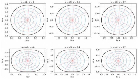
For $\sigma =0$, this definition gives the original class ${\mathfrak{MS}}_{\tan \mu }^{*}$. The geometric behavior of the function $q_{\sigma ,\mu }$ for selected values of $\mu$ and $\sigma$ is illustrated in Figure 3.

Figure 3. Images of the unit disk $\mathbb{D}$ under the function $q_{\sigma ,\mu }\left(z\right)=1+(1-\sigma )\tan \left(\mu z\right)$ for selected values of $\mu$ and $\sigma$. The black curves represent the boundary image $q_{\sigma ,\mu }(\partial \mathbb{D})$, while the blue and red curves show images of concentric circles and radial segments, respectively.

Theorem 9.

If $\mathfrak{f}\in {\mathfrak{MS}}_{\tan \mu ,\sigma }^{*}$ and $\left|z\right|=r<1$, then

$$\left|-{\displaystyle \frac{z{\mathfrak{f}}^{\prime }\left(z\right)}{\mathfrak{f}\left(z\right)}}-1\right|\le (1-\sigma )\tan \left(\mu r\right)$$

and

$$\mathfrak{Re}\left(-{\displaystyle \frac{z{\mathfrak{f}}^{\prime }\left(z\right)}{\mathfrak{f}\left(z\right)}}\right)\ge 1-(1-\sigma )\tan \left(\mu r\right).$$

Moreover, $\mathfrak{f}$ has the representation

$$\mathfrak{f}\left(z\right)={\displaystyle \frac{1}{z}}\exp \left(-(1-\sigma ){\int }_0^z{\displaystyle \frac{\tan \left(\mu \omega \right(t\left)\right)}{t}}dt\right),$$

where ω is a Schwarz function.

Proof. 

By the definition of ${\mathfrak{MS}}_{\tan \mu ,\sigma }^{*}$, there exists a Schwarz function $\omega$ such that

$$-{\displaystyle \frac{z{\mathfrak{f}}^{\prime }\left(z\right)}{\mathfrak{f}\left(z\right)}}=1+(1-\sigma )\tan \left(\mu \omega \left(z\right)\right).$$

The estimate obtained in the proof of Theorem 1 gives $\left|\tan \right(\mu \omega \left(z\right)\left)\right|\le \tan \left(\mu r\right)$. This immediately yields the modulus estimate and the real-part estimate. Finally,

$${\displaystyle \frac{d}{dz}}\log \left(z\mathfrak{f}\left(z\right)\right)=-(1-\sigma ){\displaystyle \frac{\tan \left(\mu \omega \right(z\left)\right)}{z}},$$

and integration from 0 to z gives the stated representation. □

Theorem 10.

Let $0\le \rho <1$. The ${\mathfrak{MS}}^{*}\left(\rho \right)$-radius for ${\mathfrak{MS}}_{\tan \mu ,\sigma }^{*}$ is

$$R_{{\mathfrak{MS}}^{*}\left(\rho \right)}\left({\mathfrak{MS}}_{\tan \mu ,\sigma }^{*}\right)=\min \left\{1,{\displaystyle \frac{1}{\mu }}{\tan }^{-1}\left({\displaystyle \frac{1-\rho }{1-\sigma }}\right)\right\}.$$

Proof. 

Theorem 9 shows that

$$\mathfrak{Re}\left(-{\displaystyle \frac{z{\mathfrak{f}}^{\prime }\left(z\right)}{\mathfrak{f}\left(z\right)}}\right)\ge 1-(1-\sigma )\tan \left(\mu r\right).$$

Thus $\mathfrak{f}\in {\mathfrak{MS}}^{*}\left(\rho \right)$ whenever

$$1-(1-\sigma )\tan \left(\mu r\right)\ge \rho ,$$

which is equivalent to

$$r\le {\displaystyle \frac{1}{\mu }}{\tan }^{-1}\left({\displaystyle \frac{1-\rho }{1-\sigma }}\right).$$

The radius cannot exceed 1, so the asserted expression follows. Sharpness for the nontrivial case when this number is less than 1 is obtained from

$${\mathfrak{f}}_{\sigma ,\mu }\left(z\right)={\displaystyle \frac{1}{z}}\exp \left(-(1-\sigma ){\int }_0^z{\displaystyle \frac{\tan \left(\mu t\right)}{t}}dt\right),$$

for which

$$-{\displaystyle \frac{z{\mathfrak{f}}_{\sigma ,\mu }^{\prime }\left(z\right)}{{\mathfrak{f}}_{\sigma ,\mu }\left(z\right)}}=1+(1-\sigma )\tan \left(\mu z\right).$$

At the boundary point $z=-R_{{\mathfrak{MS}}^{*}\left(\rho \right)}\left({\mathfrak{MS}}_{\tan \mu ,\sigma }^{*}\right)$, the real part equals $\rho$. □

Theorem 11.

Let $A=1-\sigma$ and $0\le \rho <1$. Every function in ${\mathfrak{MS}}_{\tan \mu ,\sigma }^{*}$ is meromorphically convex of order ρ in $\left|z\right|<R_c$, where

$$R_c=\min \{1,r_1,r_2\},r_2={\displaystyle \frac{1}{\mu }}{\tan }^{-1}\left({\displaystyle \frac{1-\rho }{A}}\right),$$

and $r_1$ is the first positive root of

$$\left(1-A\tan \mu r\right)\left(1-A\tan \mu r-\rho \right)(1-r^2)-A\mu r{\sec }^2\mu r=0.$$

Proof. 

For $\mathfrak{f}\in {\mathfrak{MS}}_{\tan \mu ,\sigma }^{*}$, write

$$-{\displaystyle \frac{z{\mathfrak{f}}^{\prime }\left(z\right)}{\mathfrak{f}\left(z\right)}}=1+A\tan \left(\mu \omega \left(z\right)\right),$$

where $\omega$ is a Schwarz function. Logarithmic differentiation gives

$$-1-{\displaystyle \frac{z{\mathfrak{f}}^{\prime \prime }\left(z\right)}{{\mathfrak{f}}^{\prime }\left(z\right)}}=1+A\tan \left(\mu \omega \left(z\right)\right)-{\displaystyle \frac{A\mu z{\omega }^{\prime }\left(z\right){\sec }^2\left(\mu \omega \left(z\right)\right)}{1+A\tan \left(\mu \omega \right(z\left)\right)}}.$$

Using $\left|\tan \right(\mu \omega \left(z\right)\left)\right|\le \tan \mu r$, $\left|\sec \right(\mu \omega \left(z\right)\left)\right|\le \sec \mu r$, and

$$|{\omega }^{\prime }\left(z\right)|\le {\displaystyle \frac{1-{\left|\omega \left(z\right)\right|}^2}{1-{\left|z\right|}^2}}\le {\displaystyle \frac{1}{1-r^2}},$$

we obtain

$$\mathfrak{Re}\left(-1-{\displaystyle \frac{z{\mathfrak{f}}^{″}\left(z\right)}{{\mathfrak{f}}^{\prime }\left(z\right)}}\right)\ge 1-A\tan \mu r-{\displaystyle \frac{A\mu r{\sec }^2\mu r}{(1-r^2)(1-A\tan \mu r)}}.$$

The right-hand side is at least $\rho$ precisely when

$$\left(1-A\tan \mu r\right)\left(1-A\tan \mu r-\rho \right)(1-r^2)-A\mu r{\sec }^2\mu r\ge 0.$$

Together with $r<r_2$, this proves the asserted convexity radius. □

Corollary 2.

Taking $\sigma =0$ in Theorems 10 and 11 recovers the corresponding radius statements for the original class ${\mathfrak{MS}}_{\tan \mu }^{*}$.

6. Conformal Mapping Theory

In this section, we record the conformal mapping interpretation of the superordinate function

$$q_0\left(z\right)=1+\tan \left(\mu z\right),0<\mu \le {\displaystyle \frac{\pi }{4}}.$$

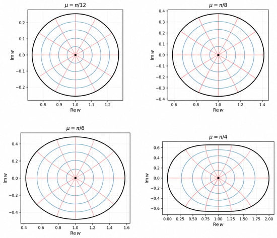
This point of view explains the geometric nature of the domain ${\omega }_{\tan \mu }$ and gives an equivalent range criterion for functions in ${\mathfrak{MS}}_{\tan \mu }^{*}$. The conformal images of the unit disk under $q_0$ for selected values of $\mu$ are shown in Figure 4.

Figure 4. Conformal images of the unit disk under $q_0\left(z\right)=1+\tan \left(\mu z\right)$ for selected values of $\mu$. The black curves represent the boundary image $q_0(\partial \mathbb{D})$, while the blue and red curves represent images of concentric circles and radial segments, respectively.

Theorem 12.

The function $q_0\left(z\right)=1+\tan \left(\mu z\right)$ is a conformal mapping of $\mathbb{D}$ onto ${\omega }_{\tan \mu }$. Moreover, the inverse function on ${\omega }_{\tan \mu }$ is

$$q_0^{-1}\left(w\right)={\displaystyle \frac{1}{\mu }}{\tan }^{-1}(w-1),$$

where ${\tan }^{-1}$ denotes the analytic branch determined by ${\tan }^{-1}\left(0\right)=0$.

Proof. 

Since $0<\mu \le \pi /4$, the disk $\mu \mathbb{D}$ is contained in the vertical strip $\{z:|\mathfrak{Re}z|<\pi /2\}$. The tangent function is one-to-one in this strip, because $\tan z_1=\tan z_2$ implies $z_1-z_2=k\pi$ for some integer k, and the strip condition forces $k=0$. Hence $q_0$ is univalent in $\mathbb{D}$. Also,

$$q_0^{\prime }\left(z\right)=\mu {\sec }^2\left(\mu z\right)\ne 0,$$

because the zeros of $\cos z$ do not meet $\mu \mathbb{D}$. Thus $q_0$ is conformal. Solving $w=1+\tan \left(\mu z\right)$ gives the asserted inverse. □

Theorem 13.

For $0<r\le 1$, let

$${\omega }_{\tan \mu }\left(r\right)=q_0\left(\{z:|z|<r\}\right).$$

Then ${\omega }_{\tan \mu }\left(r\right)$ is a simply connected Jordan domain whose boundary is parametrized by

$${\Gamma }_{\mu ,r}\left(\theta \right)=1+\tan \left(\mu r{e}^{i\theta }\right),0\le \theta \le 2\pi .$$

Equivalently, if ${\Gamma }_{\mu ,r}\left(\theta \right)=U_{\mu ,r}\left(\theta \right)+i{V}_{\mu ,r}\left(\theta \right)$, then

$$U_{\mu ,r}\left(\theta \right)=1+{\displaystyle \frac{\sin \left(2\mu r\cos \theta \right)}{\cos \left(2\mu r\cos \theta \right)+\cosh \left(2\mu r\sin \theta \right)}}$$

and

$$V_{\mu ,r}\left(\theta \right)={\displaystyle \frac{\sinh \left(2\mu r\sin \theta \right)}{\cos \left(2\mu r\cos \theta \right)+\cosh \left(2\mu r\sin \theta \right)}}.$$

Furthermore,

$$\left\{w\in \mathbb{C}:|w-1|<\tanh \left(\mu r\right)\right\}\subset {\omega }_{\tan \mu }\left(r\right)\subset \left\{w\in \mathbb{C}:|w-1|<\tan \left(\mu r\right)\right\}.$$

Proof. 

By Theorem 12, $q_0$ is conformal in a neighborhood of the closed disk $\left|z\right|\le r$ and has no self-intersection on $\left|z\right|=r$. Hence ${\Gamma }_{\mu ,r}$ is the boundary of the simply connected image domain ${\omega }_{\tan \mu }\left(r\right)$. The stated parametric form follows from

$$\tan (x+iy)={\displaystyle \frac{\sin \left(2x\right)+i\sinh \left(2y\right)}{\cos \left(2x\right)+\cosh \left(2y\right)}},$$

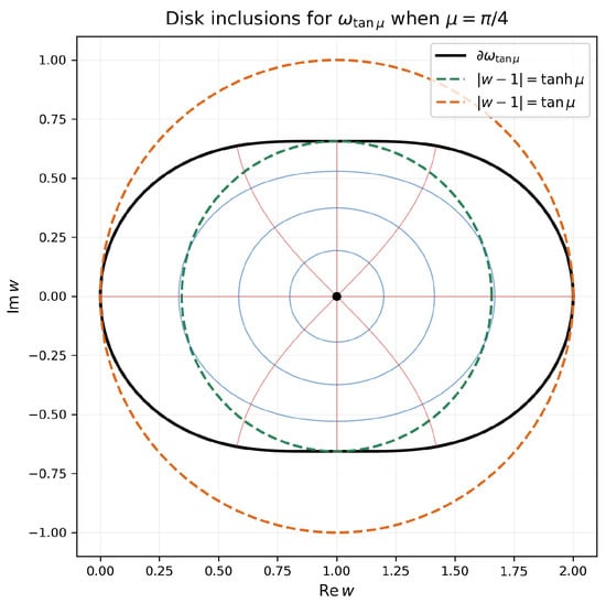
with $x=\mu r\cos \theta$ and $y=\mu r\sin \theta$. Finally, the extremal boundary distances from the point 1 are

$$\underset{0\le \theta \le 2\pi }{\min }|\tan \left(\mu r{e}^{i\theta }\right)|=\tanh \left(\mu r\right),\underset{0\le \theta \le 2\pi }{\max }\left|\tan \left(\mu r{e}^{i\theta }\right)\right|=\tan \left(\mu r\right),$$

as obtained by the same calculation used in Theorem 1 and Lemma 3. The two disk inclusions follow at once. □

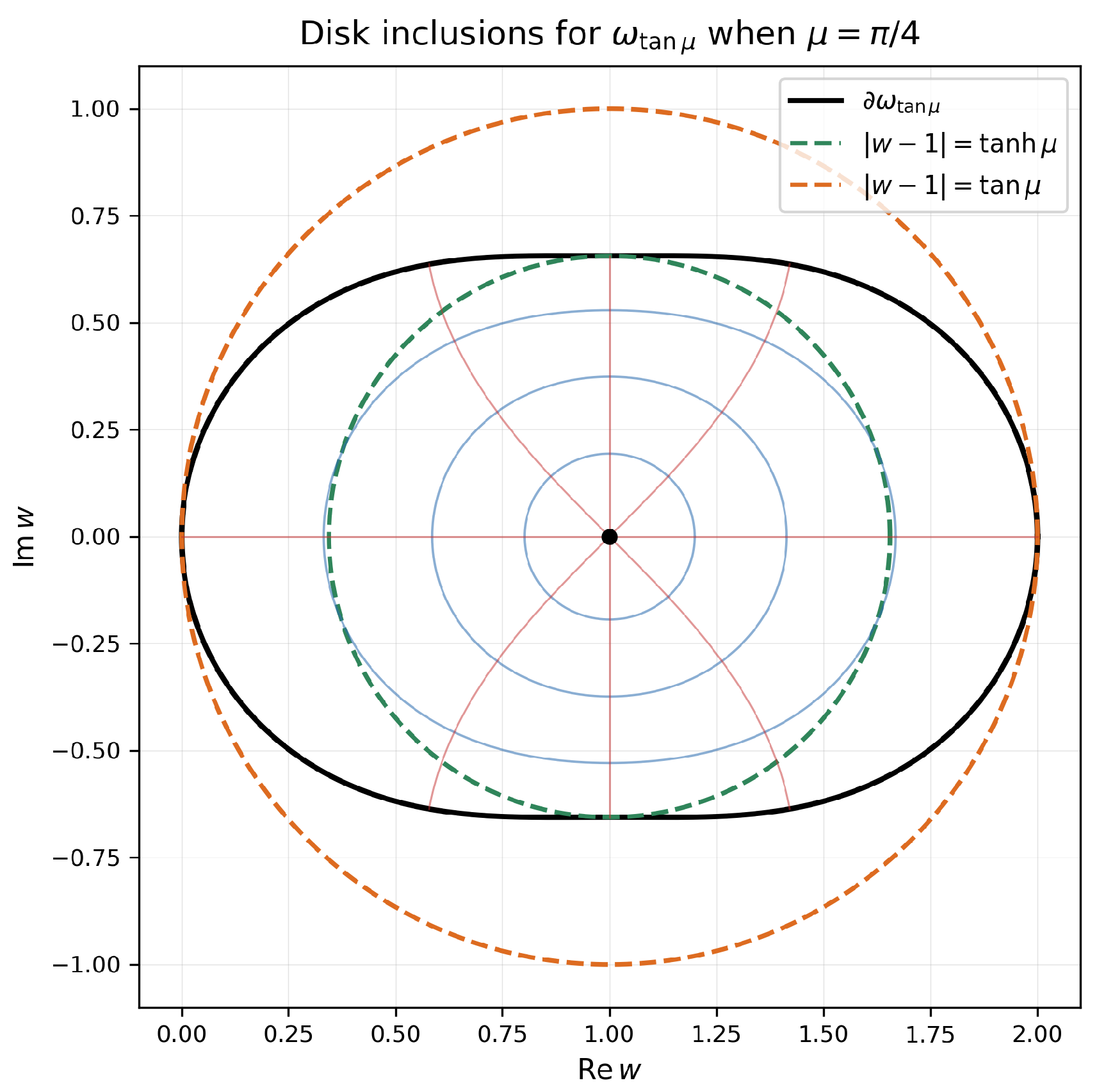
The disk inclusions used in the radius estimates are illustrated in Figure 5.

Figure 5. The conformal image domain ${\omega }_{\tan \mu }$ for $\mu =\pi /4$ together with the inner disk $|w-1|<\tanh \mu$ and the outer disk $|w-1|<\tan \mu$. This illustrates the disk inclusions used in the radius estimates.

Theorem 14.

Let $\mathfrak{f}\in \mathfrak{M}$ be such that

$$p_{\mathfrak{f}}\left(z\right)=-{\displaystyle \frac{z{\mathfrak{f}}^{\prime }\left(z\right)}{\mathfrak{f}\left(z\right)}}$$

is analytic in $\mathbb{D}$ and satisfies $p_{\mathfrak{f}}\left(0\right)=1$. Then

$$\mathfrak{f}\in {\mathfrak{MS}}_{\tan \mu }^{*}$$

if and only if

$$p_{\mathfrak{f}}\left(\mathbb{D}\right)\subset {\omega }_{\tan \mu }.$$

Equivalently,

$${\Omega }_{\mathfrak{f}}\left(z\right)={\displaystyle \frac{1}{\mu }}{\tan }^{-1}\left(p_{\mathfrak{f}}\left(z\right)-1\right)$$

is a Schwarz function.

Proof. 

Since $q_0$ is univalent by Theorem 12 and $q_0\left(0\right)=1$, the standard subordination principle for univalent functions gives

$$p_{\mathfrak{f}}\prec q_0⟺p_{\mathfrak{f}}\left(0\right)=q_0\left(0\right)\mathrm{and}{p}_{\mathfrak{f}}\left(\mathbb{D}\right)\subset q_0\left(\mathbb{D}\right).$$

The equivalence follows because $q_0\left(\mathbb{D}\right)={\omega }_{\tan \mu }$. Applying the inverse map from Theorem 12 gives the Schwarz function ${\Omega }_{\mathfrak{f}}=q_0^{-1}\circ p_{\mathfrak{f}}$. □

Remark 1.

If $\mathfrak{f}\left(z\right)=h\left(z\right)/z$, where $h\left(0\right)=1$ and h is analytic and nonzero in $\mathbb{D}$, then

$$p_{\mathfrak{f}}\left(z\right)=1-{\displaystyle \frac{z{h}^{\prime }\left(z\right)}{h\left(z\right)}},$$

which shows that the analyticity assumption in Theorem 14 is automatic for this nonvanishing normalized factor.

Corollary 3.

Let $\mathfrak{f}\in \mathfrak{M}$ and suppose that, for $\left|z\right|<r$,

$$\left|p_{\mathfrak{f}}\left(z\right)-1\right|<\tanh \mu .$$

Then $\mathfrak{f}$ belongs to ${\mathfrak{MS}}_{\tan \mu }^{*}$ in the disk $\left|z\right|<r$. More generally, if

$$\left|p_{\mathfrak{f}}\left(z\right)-1\right|<\tanh \left(\mu s\right),0<s\le 1,$$

for $\left|z\right|<r$, then $p_{\mathfrak{f}}\left(\right|z|<r)\subset {\omega }_{\tan \mu }\left(s\right)$.

Proof. 

The result follows immediately from the disk inclusion in Theorem 13 and the conformal range criterion of Theorem 14. □

7. Conclusions

In the present paper, we have defined and studied the new class ${\mathfrak{MS}}_{\tan \mu }^{*}$ of meromorphic starlike functions in terms of subordination to the generalized tangent function. Radii of starlikeness and convexity were determined. Also, some radius results have been proved for various well-known subclasses, such as Janowski-type classes and quotient classes of meromorphic functions. A new subclass ${\mathfrak{MS}}_{\tan \mu ,\sigma }^{*}$ of tangent order has been defined, whose representation formula has been derived, and radius estimates of starlikeness and convexity have been obtained.

Moreover, we have studied the mapping properties of the superordinate function $q_0\left(z\right)=1+\tan \left(\mu z\right)$. In particular, we have analyzed its inverse function, parametrization of its boundary, image-domain inclusions, and conformal range criterion.

This paper opens up different areas of future research on this new subclass, such as coefficient inequalities, distortion theorems, Hankel determinants, extremal problems, inclusion relations, and differential subordinations problems.

References

- Clunie, J. On meromorphic schlicht functions. J. Lond. Math. Soc. 1959, 1, 215–216. [Google Scholar] [CrossRef] [Scilit]
- Libera, R.J.; Robertson, M.S. Meromorphic close-to-convex functions. Mich. Math. J. 1961, 8, 167–175. [Google Scholar] [CrossRef] [Scilit]
- Pommerenke, C. Über einige klassen meromorpher schlichter funktionen. Math. Z. 1962, 78, 263–284. [Google Scholar] [CrossRef] [Scilit]
- Royster, W.C. Meromorphic starlike multivalent functions. Trans. Am. Math. Soc. 1963, 107, 300–308. [Google Scholar] [CrossRef] [Scilit]
- Miller, J. Convex meromorphic mappings and related functions. Proc. Am. Math. Soc. 1970, 25, 220–228. [Google Scholar] [CrossRef] [Scilit]
- Goel, R.M.; Sohi, N.S. On a class of meromorphic functions. Glas. Mat. 1981, 17, 19–28. [Google Scholar]
- Khan, N.; Arif, M.; Darus, M. Majorization properties for certain subclasses of meromorphic function of complex order. Complexity 2022, 2022, 2385739. [Google Scholar] [CrossRef] [Scilit]
- Tayyah, A.S.; Atshan, W.G.; Oros, G.I. Third-order differential subordination results for meromorphic functions associated with the inverse of the Legendre chi function via the Mittag-Leffler identity. Mathematics 2025, 13, 2089. [Google Scholar] [CrossRef] [Scilit]
- Alatawi, A.; Darus, M. Partial sums and neighborhoods of Janowski-type subclasses of meromorphic functions. Korean J. Math. 2023, 31, 259–267. [Google Scholar]
- Srivastava, H.M.; Arif, M.; Raza, M. Convolution properties of meromorphically harmonic functions defined by a generalized convolution q-derivative operator. AIMS Math. 2021, 6, 5869–5885. [Google Scholar] [CrossRef] [Scilit]
- Shah, S.G.A.; Hussain, S.; Rasheed, A.; Shareef, Z.; Darus, M. Application of quasisubordination to certain classes of meromorphic functions. J. Funct. Spaces 2020, 2020, 4581926. [Google Scholar] [CrossRef] [Scilit]
- He, T.; Li, S.-H.; Ma, L.-N.; Tang, H. Closure properties of generalized λ-Hadamard product for a class of meromorphic Janowski functions. AIMS Math. 2021, 6, 1715–1726. [Google Scholar] [CrossRef] [Scilit]
- Ali, R.M.; Ravichandran, V. Classes of meromorphic α-convex functions. Taiwan J. Math. 2010, 14, 1479–1490. [Google Scholar] [CrossRef] [Scilit]
- Wang, Z.-G.; Farooq, M.U.; Arif, M.; Malik, S.N.; Tawfiq, F.M.O. A class of meromorphic functions involving higher order derivative. J. Contemp. Math. Anal. 2024, 59, 419–429. [Google Scholar] [CrossRef] [Scilit]
- Kwon, O.S.; Sim, Y.J.; Cho, N.E.; Srivastava, H.M. Some radius problems related to a certain subclass of analytic functions. Acta Math. Sin. Engl. Ser. 2014, 30, 1133–1144. [Google Scholar] [CrossRef] [Scilit]
- Cho, N.E.; Kim, I.; Srivastava, H.M. New criteria for functions in a class of meromorphically strongly starlike functions. Anal. Stiint. Univ. Ovidius Constanta Ser. Mat. 2024, 32, 57–73. [Google Scholar] [CrossRef] [Scilit]
- Ali, R.M.; Jain, N.K.; Ravichandran, V. Radii of starlikeness associated with the Lemniscate of Bernoulli and the left-half plane. Appl. Math. Comput. 2012, 218, 6557–6565. [Google Scholar] [CrossRef] [Scilit]
- Tayyah, A.S.; Atshan, W.G. Starlikeness and bi-starlikeness associated with a new Carathéodory function. J. Math. Sci. 2025, 290, 232–256. [Google Scholar] [CrossRef] [Scilit]
- Sharma, K.; Jain, N.K.; Ravichandran, V. Starlike functions associated with a cardioid. Afr. Mat. 2016, 27, 923–939. [Google Scholar] [CrossRef] [Scilit]
- Cho, N.E.; Kumar, V.; Kumar, S.S.; Ravichandran, V. Radius problems for starlike functions associated with the sine function. Bull. Iran. Math. Soc. 2019, 45, 213–232. [Google Scholar] [CrossRef] [Scilit]
- Tayyah, A.S.; Hadi, S.H.; Wang, Z.-G.; Lupaş, A.A. Classes of Ma–Minda type analytic functions associated with a kidney-shaped domain. AIMS Math. 2025, 10, 22445–22470. [Google Scholar] [CrossRef] [Scilit]
- Shah, G.M. On the univalence of some analytic functions. Pac. J. Math. 1972, 43, 239–250. [Google Scholar] [CrossRef] [Scilit]
- Ravichandran, V.; Rønning, F.; Shanmugam, T.N. Radius of convexity and radius of starlikeness for some classes of analytic functions. Complex Var. Theory Appl. 1997, 33, 265–280. [Google Scholar] [CrossRef] [Scilit]
Disclaimer/Publisher’s Note: The statements, opinions and data contained in all publications are solely those of the individual author(s) and contributor(s) and not of MDPI and/or the editor(s). MDPI and/or the editor(s) disclaim responsibility for any injury to people or property resulting from any ideas, methods, instructions or products referred to in the content. |
© 2026 by the authors. Licensee MDPI, Basel, Switzerland. This article is an open access article distributed under the terms and conditions of the Creative Commons Attribution (CC BY) license.