


Abstract
Field magnetotelluric (MT) observation data confirmed the widespread existence of electrical anisotropy in the mid-lower crust and upper-mantle regions. Several potential electric transport mechanisms, such as the mineralogical fabric, the lithologic layering, the preferential alignment of fluid or melt, etc., have been put forward to reasonably explain the anisotropic electrical conductivity. However, the detailed contributions of each mechanism to rock-scale electrical anisotropy are difficult to quantify using laboratory-based electrical conductivity measurements. Herein, we develop GeoAnisoLab, an absolutely new numerical modeling program to characterize the anisotropic electrical conductivity of rocks at high temperature and high pressure. It integrates crystallographic preferred orientations, mineral conductivity data, and resistor-network modeling by constructing five typical petrological models (i.e., a randomly distributed rock model, two lithologically layered models, a fluid-bearing layered model, and a melt-bearing layered model). In comprehensive considerations of previously available high-pressure experimental and filed MT results, the GeoAnisoLab numerical modeling method can systematically assess the anisotropic conductivity anomalies in the deep Earth.
1. Introduction
Anisotropic electrical conductivity in the deep Earth’s interior has been widely detected by magnetotelluric (MT) sounding results [1,2,3]. It is commonly attributed to the mineralogical fabric, the lithologic layering, the preferential alignment of fluid or melt, etc. [4,5,6,7]. Previous experimental conductivity studies have demonstrated that single-crystal quartz and plagioclase can exhibit pronounced electrical anisotropy in the mid-lower crustal region [8,9,10]. When we convert the electrical anisotropy from the mineral single crystal to polycrystalline aggregates, it strongly depends on the crystallographic preferred orientations (CPO) [4]. However, the magnitude of petrological electrical anisotropy is substantially reduced [4,11]. Therefore, it is obvious that electrical anisotropy of mineral single crystal cannot be applied directly to explain the geophysical observed anisotropy anomalies. On the other hand, it is difficult to quantify the detailed contributions for each electrical anisotropy mechanism of rocks from these laboratory-based electrical conductivity measurements at high temperature and high pressure. In most cases, the genuine sample constituent capable of systematically characterizing anisotropic mechanisms in the deep Earth’s interior is not easy to be obtained by the high-temperature and high-pressure experiments.
Numerical modeling provides a feasible method for quantifying rock-scale electrical anisotropy. Conventional theoretical models have been adopted to calculate the bulk electrical conductivity of geomaterials, such as Hashin-Shtrikman bounds (HS), series-parallel models, and geometric mean models [12,13,14,15]. By combining these theoretical models with experimental electrical conductivity data for rock-forming minerals and fluids/melts [15,16,17,18], computational tools such as SIGMELTS have been developed to assess the isotropic conductivity at high temperature and high pressure [19]. Nevertheless, these available computational tools are not designed to evaluate rock-scale electrical anisotropy. More recently, the network-based models provide a valid approach for simulating the anisotropic electrical conductivity of rocks and identify which anisotropic conductivity mechanisms to reasonably interpret geophysically observed electrical anisotropy [4,11,20,21]. However, these models have not yet been incorporated into a dedicated program platform. Therefore, a software tool that directly calculates rock electrical anisotropy is needed to make the modeled results more accessible to the geophysical community.
Herein, we developed an interactive software (GeoAnisoLab) for calculating the electrical conductivity anisotropy of rock under conditions relevant to the Earth’s crust and upper mantle. By integrating mineralogical conductivity data, crystallographic orientations, mineralogical assemblages, and preferentially aligned fluids/melts, the GeoAnisoLab software quantitatively evaluates the effects of different mechanisms on rock electrical anisotropy. This software allows users to construct randomly distributed, lithologically layered, fluid-bearing, and melt-bearing rock models. The main input parameters are temperature, mineralogy, crystallographic fabric, and the composition and abundance of fluids/melts. The outputs include the electrical anisotropy ratio and visualizations of the simulated resistor networks. By comparing the simulated electrical anisotropy with that inferred from MT data, users can assess which geological mechanisms are capable of reproducing the observed electrical anisotropy.
2. Software Development and Computational Detail
The GeoAnisoLab (version 1.0) software is designed by the random resistor network method, and the calculating program is developed on the basis of Luo et al. [11] at high temperature and high pressure. As usual, users need to set the model parameters, after which the GeoAnisoLab software makes it relatively easy to construct the resistor networks and automatically calculates the electrical anisotropy of rocks. The user interface was constructed using TypeScript 7.0.2, React 19.2.7, and Electron 43.1.0, while the computational components were integrated into Python 3.9.7. This software is packaged as an independent executable file and can therefore be run directly without installing Node.js or Python. The GeoAnisoLab framework is organized into four main computational modules: parameter input, data retrieval, resistor-network construction, and calculation/output visualization. In the module of parameter input, users define temperature, mineral assemblage, modal proportion, crystallographic fabric, and fluid/melt parameters when applicable. In the module of data retrieval, the program reads mineral conductivity data and CPO information from the built-in database or from user-uploaded files. In the module of resistor-network construction, the selected simulation option determines how mineral phases, lithologic layers, and conductive fluids or melts are arranged in the resistor network. Finally, the calculation/output module simulates the electric currents in two orthogonal directions, calculates the electrical anisotropy ratio, and visualizes the corresponding circuit structures.
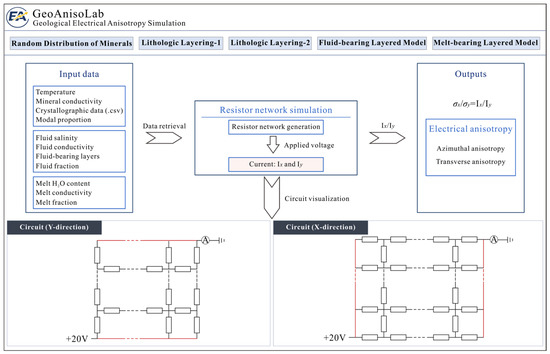
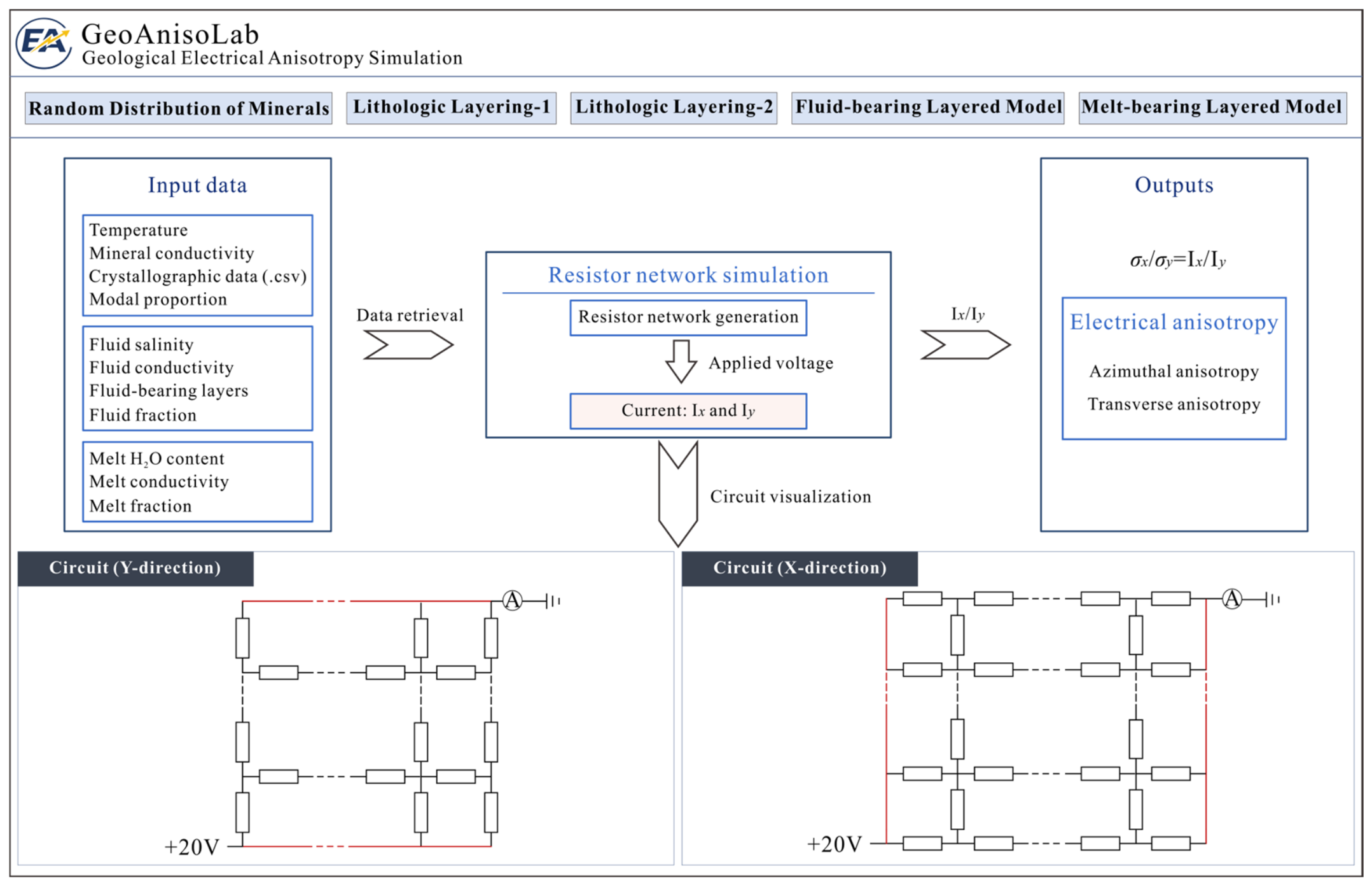
The schematic interface and calculation workflow of GeoAnisoLab software are shown in Figure 1 in detail. The five simulation options in the user interface, including “Random Distribution of Minerals”, “Lithologic Layering—1”, “Lithologic Layering—2”, “Fluid-Bearing Layered Model”, and “Melt-Bearing Layered Model”, correspond to different resistor-network construction modules. These options differ in model architecture, but they follow the same calculation workflow. The upper panels are designed for model selection, parameter input, and result output, whereas the lower panels visualize circuit simulations along two orthogonal directions. Each corresponding resistor network is composed of 400 resistor pairs.
Figure 1.
Schematic interface and calculation workflow of GeoAnisoLab software. The workflow consists of parameter input, data retrieval, resistor-network construction, electrical calculation, and output visualization. The five simulation options correspond to different resistor-network construction modules. All models then adopt the same electrical calculation and visualization procedures. The lower panels display the corresponding circuit simulations in the X and Y directions, the red boundary lines represent short-circuited electrodes used to apply a voltage across the resistor network.
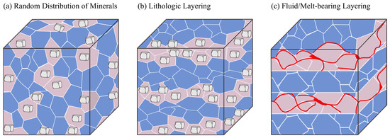
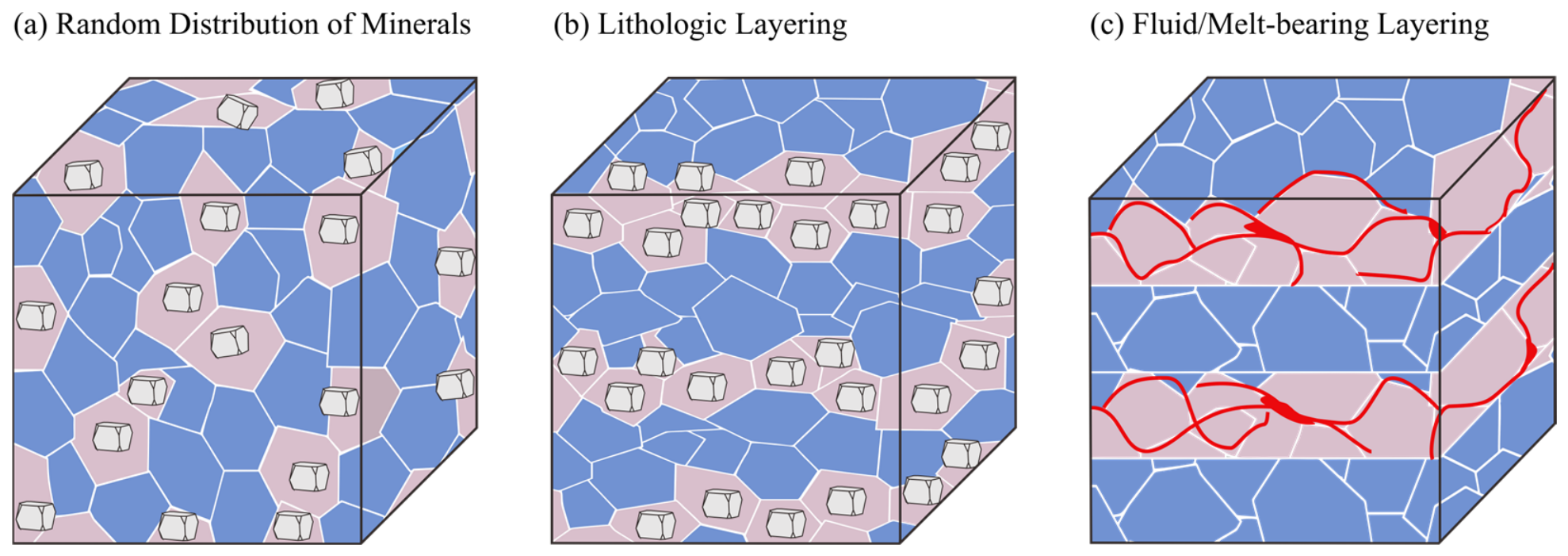
To better illustrate the structural assumptions of the models implemented in the GeoAnisoLab software, schematic cartoons of the model structures are shown in Figure 2. It demonstrates how mineral phases are distributed in the randomly distributed model, how layered structures are arranged in the lithologic layering models, and how fluids and melts are localized in predefined sub-layers in the fluid/melt-bearing model.
Figure 2.
Schematic illustration of electrical anisotropy models. (a) Random distribution of minerals, in which different mineral phases are dispersed throughout the model. (b) Lithologic layering, in which different lithologic minerals are arranged as laterally continuous layers. (c) Fluid/melt-bearing model, in which conductive fluids or melts are preferentially connected along specific layers. The red curves represent connected fluid/melt pathways.
2.1. Input Parameters
In the parameter-input module, users first select a simulation option and then set the temperature, mineralogical assemblages, and proportions. Pressure is not considered since its effect on mineral conductivity is negligible relative to that of temperature [9,22]. The volume fraction of each phase can be input individually, which allows users to construct single-phase, two-phase, or three-phase rock models.
The anisotropic mineral phase can be selected from the built-in database (Table 1). The three conductivity values along the principal crystallographic directions of the selected mineral are then retrieved automatically. Users can also input these values manually when the target mineral phase is not available in the database. In the current version, the three directional conductivities must be input in the following order: [uvw], [rst], and [hkl]. Crystallographic orientation data can be selected from the database or updated as a CSV file. The last three columns of CSV file are configured as the Euler angles [23]. The second and third mineralogical phases are treated as electrically isotropic and are therefore assigned a direction-independent conductivity value. These conductivity values can be selected from the database or input manually. In the “Random Distribution of Minerals” model, this randomization controls only the spatial positions of the mineral phases. The crystallographic orientations of anisotropic minerals are prescribed by the selected or uploaded CPO data.
Table 1.
The data sources used in the calculations.
The GeoAnisoLab software includes two types of layered models, each of which has a predefined structural assumption. These two models are designed to represent different natural lithologic structures. The total number of resistor pairs is fixed at 400 in both models, whereas the number of layers and the allocation of resistor pairs within individual layers vary according to the target lithologic structure. The “Lithologic Layering—1” model consists of nine layers. The corresponding numbers of resistor pairs in successive layers are 20, 60, 20, 80, 20, 80, 20, 80, and 20. The isotropic mineral phases are distributed proportionally within layers 2, 4, 6, and 8. In this model, the total proportion of anisotropic mineral phases must exceed 25%. This configuration is designed to reproduce interlayering between monomineralic quartz layers and polymineralic quartz-bearing layers. It is therefore suitable for quartz-rich crustal rocks in which compositional layering occurs at the rock scale. In contrast, the “Lithologic Layering—2” model is composed of seven layers with a different geometric arrangement. From the first to the seventh layer, the numbers of resistor pairs are 80, 40, 80, 40, 80, 40, and 40, respectively. This configuration is designed based on the xenoliths from lower-crustal rocks with alternating pyroxene-rich and plagioclase-rich layers. To represent compositional layering, the overall proportion of anisotropic mineral phases is fixed at 62%, while their proportions in successive layers alternate following the sequence 80–20–80–20–80–20–80 vol.%. The isotropic mineral phases are randomly distributed throughout the remaining parts of the resistor network.
In the fluid-bearing layered model, users can specify fluid types (NaCl-bearing fluid or custom), salinities, fluid-bearing layers (odd- or even-numbered layers), and fluid fractions. As illustrated in Figure 2c, this model follows a layered structure in which fluids are assigned to selected layers. Owing to the weakening effect of fluids on microfabrics of matrix [24], the crystallographic orientations are not taken into account in the fluid-bearing layers. Accordingly, the conductivity of the fluid-bearing layer is calculated using the HS+ model based on the conductivities of saline fluids and solid matrix [12,32,36]. The crystallographic orientations are considered only in fluid-free layers. In the melt-bearing layered model (Figure 2c), melt is fixed at the predefined even-numbered layers and is localized within a single sub-layer rather than occupying the entire even-numbered layers. Users can specify the melt types (peraluminous granitic, basaltic, carbonatitic, or custom), melt H2O content, and melt fractions. The option of basaltic melt is restricted to a temperature range of 1473–1923 K. Although fluids and melts are both treated as highly conductive phases in the GeoAnisoLab software, they are parameterized separately because their controlling factors are different. The fluid-bearing model is controlled mainly by fluid salinity, fluid fraction, and the choice of fluid-bearing layers. By contrast, the melt-bearing model is controlled by melt composition, H2O content, and melt fraction.
2.2. Output and Visualization
In the calculation/output module, the GeoAnisoLab software provides two calculation modes: azimuthal anisotropy and transverse anisotropy. Azimuthal anisotropy describes the conductivity contrast between two orthogonal horizontal directions, while transverse anisotropy refers to the contrast between the vertical and horizontal directions. After selecting the calculation mode, the calculation is initiated by clicking the “Run compute” button. The software then constructs two resistor networks to simulate conductance along two orthogonal directions. The same voltage is applied across both networks. The effective conductance in each direction is determined from the simulated current. Because the applied voltage, network geometry, and mineral distribution are identical in both networks, the electrical anisotropy is obtained from the ratio of the simulated currents along the two orthogonal directions (). The output panel shows the calculated anisotropy value together with a schematic diagram of the selected model. The lower part of the interface displays the two resistor networks used to simulate currents, which are visualized using CircuitJS, an online electronic-circuit simulator (https://lushprojects.com/circuitjs/ accessed on 11 July 2026).
In the GeoAnisoLab software, mineralogical phases (described as the resistor pairs) are distributed randomly in the resistor network models according to the prescribed proportions. Consequently, the repeated calculations with the same input parameters may produce slightly different anisotropic values. Each click of the “Run compute” button generates a new random resistor network and performs one calculation. To reduce the variability introduced by randomization of phase distributions, users should perform multiple calculations and average the simulated electrical anisotropy.
2.3. Model Assumptions and Uncertainties
The main assumptions and uncertainties of the resistor-network approach have been discussed in detail by Luo et al. [11]. Here, we briefly summarize the uncertainty sources most relevant to the GeoAnisoLab software. First, the input conductivity data are derived mainly from high-temperature and high-pressure experiments. These experimental values may vary because mineral, fluid, and melt conductivities are affected by temperature, pressure, water content, Fe content, oxygen fugacity, salinity, melt composition, and experimental calibration. Second, the modeled anisotropy is affected by the CPO data used for anisotropic mineral phases. In the GeoAnisoLab software, representative EBSD datasets are used as input, but the strength and type of CPO in natural rocks may vary with temperature, pressure, deformation regime, water content, and mineral composition. Therefore, different CPO inputs may produce different anisotropy values. Third, simplified assumptions on mineral distribution, compositional layering, and oriented fluid/melt pathways may not fully reproduce the complexity of natural rocks. Moreover, the numerical errors of the resistor-network calculation arise mainly from random distribution of resistor pairs, boundary artifacts, and finite network size. Previous tests indicate that the combined numerical error associated with these factors is less than 10% [11].
3. Electrical Anisotropy of Rock Models
3.1. Randomly Distributed Rock Models
In the solid-state rocks, electrical anisotropy is controlled mainly by the intrinsic conductivity of minerals, crystallographic preferred orientations, and mineral modal proportions. The randomly distributed rock model is therefore used to evaluate the contributions of these controlling factors to rock electrical anisotropy (Figure 2a). Accordingly, the required input parameters include temperature, the electrical conductivities of the constituent minerals, the crystallographic orientations, and the mineralogical proportions (Figure 1). The crystallographic orientation and conductivity data can be obtained from the built-in database, which currently collects quartz, plagioclase, amphibole, clinopyroxene, orthopyroxene, and olivine [9,10,22,24,25,26,27,28,29,30,31].
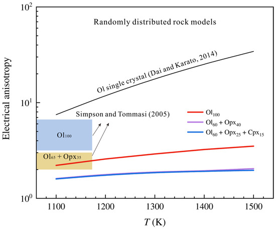
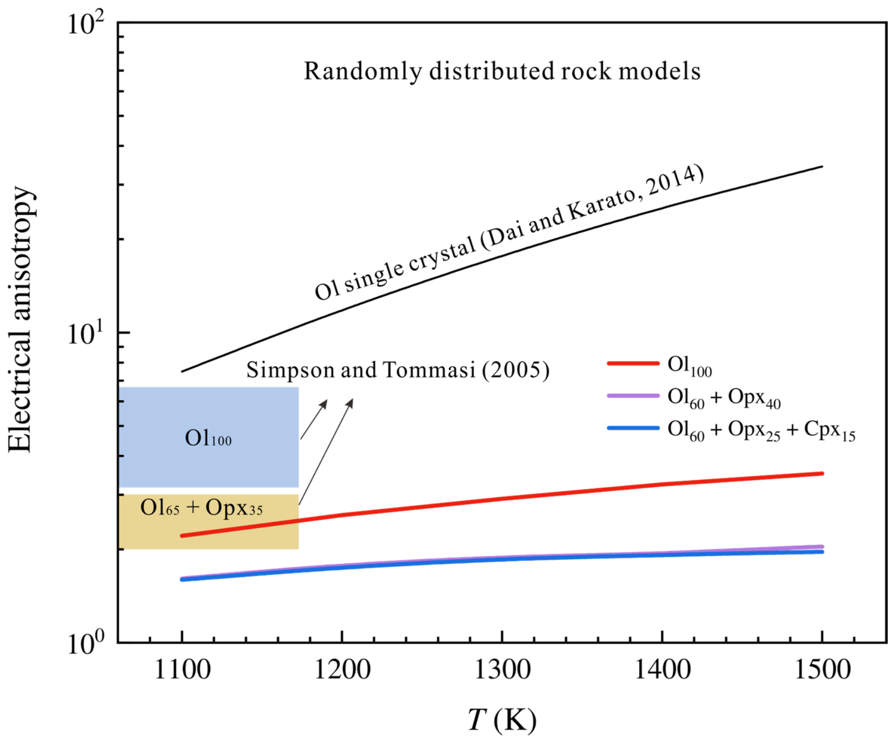
Taking peridotite as an example, three representative mineral assemblages are considered, including the single-phase olivine aggregates (Ol100), the two-phase olivine–orthopyroxene aggregates (Ol60 + Opx40), and the three-phase olivine–orthopyroxene–clinopyroxene aggregates (Ol60 + Opx25 + Cpx15). As shown in Figure 3, although olivine single crystals exhibit extremely high electrical anisotropy (10–40), the conversion from single crystals to polycrystalline aggregates substantially reduces the 2–3 anisotropic magnitude. The addition of weakly anisotropic minerals further decreases the electrical anisotropy, consistent with previous calculations for mantle peridotite [4]. Nevertheless, the calculated electrical anisotropic values are lower than those of reported results by Simpson and Tommasi [4]. Their higher values may result from the hydrogen diffusion coefficients as a proxy for the electrical conductivity of single crystals. Because the hydrogen diffusion in olivine is highly anisotropic, its conversion to conductivity through the Nernst–Einstein equation can overestimate the magnitude of electrical anisotropy. By contrast, the conductivities employed in the GeoAnisoLab software are taken from experimental measurements [29] and thus provide a more direct constraint on the electrical anisotropy of rock.
Figure 3.
Electrical anisotropy of randomly distributed rock models as a function of temperature. Red, purple, and blue curves represent the calculated anisotropy for Ol100, Ol60 + Opx40, and Ol60 + Opx25 + Cpx15 aggregates, respectively. The black curve shows the electrical anisotropy of olivine single crystals from Dai and Karato [29]. The blue and yellow shaded areas indicate the electrical anisotropy ranges reported by Simpson and Tommasi [4] for Ol100 and Ol65 + Opx35 aggregates, respectively. Abbreviations: Ol: olivine, Opx: orthopyroxene, Cpx: clinopyroxene.
Although the temperature significantly affects the calculated electrical anisotropy, crystallographic orientations remain the primary controlling factor. Strong alignment of the crystallographic axes also aligns the high-conductivity directions of the grains, thereby partially preserving the single-crystal anisotropy at the aggregate scale. In contrast, the dispersed crystallographic orientations weaken this effect through directional averaging [4,37]. Mineralogical proportions also influence the electrical anisotropy of the aggregates. As the proportions of orthopyroxene and clinopyroxene increase, the contribution of olivine is progressively weakened, thereby decreasing the electrical anisotropy of aggregate. In summary, this example illustrates how the GeoAnisoLab software combines mineralogical conductivity, crystallographic orientation, and modal proportion in the calculation of rock electrical anisotropy.
3.2. Lithologically Layered Models
The lithologic layering has been proposed as a possible source of the geophysically observed electrical anisotropy in the crust [5,6,26]. In this study, two types of lithologic layering are considered. One is interlayering between monomineralic quartz layers and polymineralic quartz-bearing layers [38]. The other is alternating pyroxene-rich and plagioclase-rich layering, as observed in granulite xenoliths from the lower continental crust [39,40]. The conductivity contrast between these compositionally distinct layers may therefore generate electrical anisotropy [26]. The GeoAnisoLab software provides two layered models with different geometric configurations. Their representative layered structures are shown in Figure 2b.
The “Lithologic Layering—1” model is designed to represent quartz-rich layered rocks. It consists of alternating monomineralic quartz layers and mixed quartz–plagioclase layers, giving a bulk composition of Qtz40 + Plag60. The electrical conductivity of quartz and plagioclase is selected from the built-in database, and its crystallographic preferred orientation is prescribed by the corresponding quartz CPO data. Plagioclase is treated as an isotropic phase in the mixed layers. The “Lithological Layering—2” is designed to quantify the contribution of plagioclase–pyroxene layering to crustal electrical anisotropy. This model is composed of 62% plagioclase, characterized by the [001] slip system, and 38% clinopyroxene. These mineralogical phases are alternately arranged to form alternating pyroxene-rich (Cpx80 + Plag20) and plagioclase-rich (Cpx20 + Plag80) layers. As the input parameters, the anisotropic electrical conductivity of plagioclase (135 ppm water) is selected from the built-in database, while the isotropic conductivity of clinopyroxene (270 ppm water) is input manually using the data of Yang and McCammon [41].
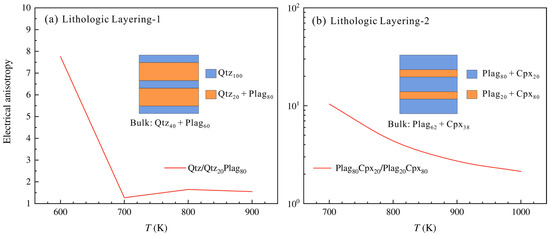
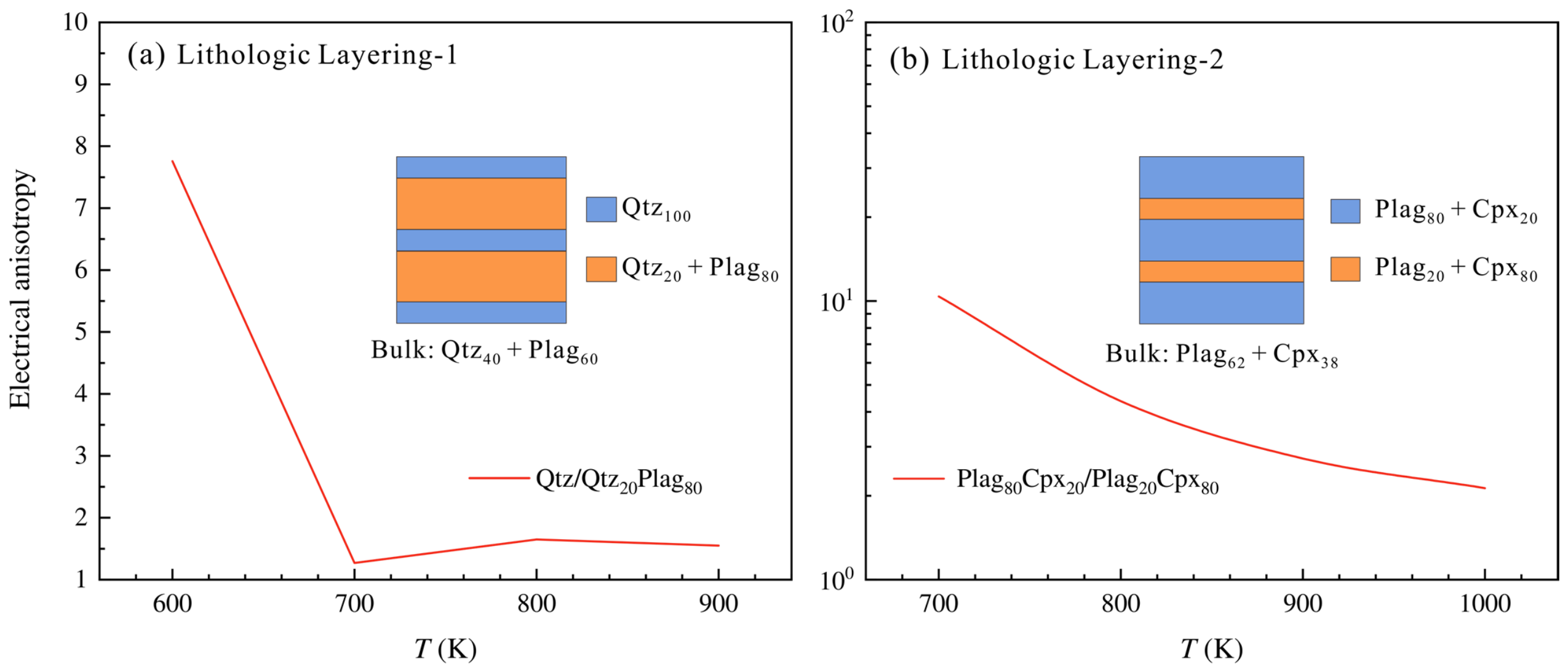
The calculated results are shown in Figure 4. Lithologic Layering-1 produces relatively high electrical anisotropy of ~8 at 600 K, but the anisotropy decreases sharply at 700 K and remains low at higher temperatures (Figure 4a). This non-monotonic variation mainly results from the quartz CPOs that evolved with temperature. Because quartz is the only anisotropic mineral phase in this model, variations in quartz CPOs modify the alignment of the high-conductivity crystallographic directions. This changes the conductivity contrast between the monomineralic quartz layers and the mixed quartz–plagioclase layers, leading to the irregular temperature dependence of electrical anisotropy. In contrast, Lithologic Layering—2 produces an electrical anisotropy of approximately 10 at relatively low temperatures (Figure 4b), which implies that the moderate electrical anisotropy observed in the lower crust may be explained by lithologic layering [11]. The calculated anisotropy decreases with temperature due to the reduced conductivity contrast between the pyroxene-rich and plagioclase-rich layers. This decrease makes it difficult to reproduce the electrical anisotropy observed in the deeper crustal regions. Moreover, the addition of a third mineral phase could further reduce the calculated electrical anisotropy. Nonetheless, this example demonstrates how the GeoAnisoLab software can be used to quantify the contribution of lithologic layering to electrical anisotropy. It can also be used to assess whether layered rocks could account for the electrical anisotropy inferred from MT observations.
Figure 4.
Electrical anisotropy of the lithologically layered model as a function of temperature. (a) Lithologic Layering—1, consisting of monomineralic quartz layers (Qtz100) and mixed quartz–plagioclase layers (Qtz20 + Plag80). For this model, different quartz CPOs were assigned at different temperatures according to the dominant slip systems: basal <a> at 600 K, rhomb <b> at 700 K, and prism <a> at 800–900 K. (b) Lithologic Layering—1 consists of alternating plagioclase-rich (Plag80 + Cpx20) and clinopyroxene-rich layers (Plag20 + Cpx80). The schematic diagram illustrates the layer configuration used in the calculation. Abbreviations: Qtz: Quartz, Plag: plagioclase, Cpx: clinopyroxene.
3.3. Fluid-Bearing Layered Models
Saline fluids are commonly regarded as a primary cause of high-conductivity anomalies in the crust and upper mantle [18,32,36,42]. Fluids can also result in electrical anisotropy when their distribution is preferentially aligned [5,6,43]. However, experimental quantification of this effect is extremely challenging due to the anomalously high mobility of fluids. Therefore, the fluid-bearing model in the GeoAnisoLab software provides a means of assessing whether aligned fluids can generate electrical anisotropy.
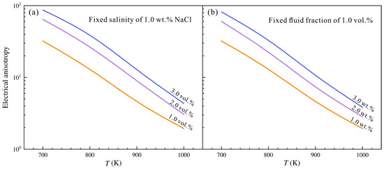
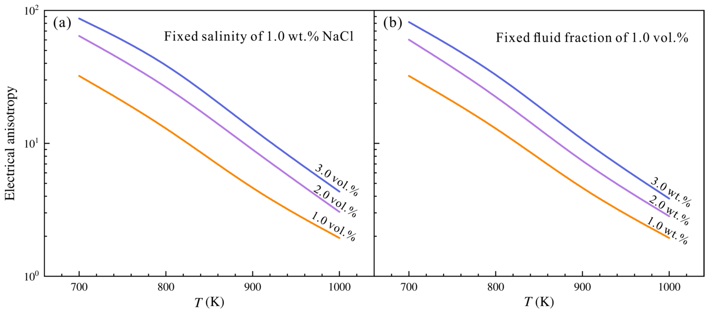
In this model, fluids can be assigned only to either the odd-numbered or even-numbered mineral layers. NaCl-bearing fluids are provided as the default fluid type. Figure 5 presents an example based on the mineral assemblage of gabbro. The solid-state matrix is same as that used in the layered model in Section 3.2. The calculated results show that preferentially aligned fluids can generate strong electrical anisotropy. At a fixed salinity of 1 wt.% NaCl, the electrical anisotropy increases markedly with fluid volume fraction from 1 to 3 vol.% (Figure 5a). For instance, the electrical anisotropy increases from approximately 32 to 87 at 1100 K. This result indicates that even a small increase in fluid fraction can substantially enhance the electrical anisotropy. At a fixed fluid fraction of 1 vol.%, increasing salinity also strongly enhances the electrical anisotropy (Figure 5b). Nevertheless, the electrical anisotropy calculated from fluid-bearing layered rocks decreases with temperature because the conductivity contrast between the fluid-bearing and fluid-free layers also decreases accordingly. In sum, this example illustrates that the GeoAnisoLab software provides a practical tool for quantifying the contribution of aligned saline fluids to electrical anisotropy. It also allows users to compare the electrical anisotropy predicted by fluid-free and fluid-bearing layered models under identical conditions.
Figure 5.
Electrical anisotropy of fluid-bearing layered gabbro models as a function of temperature. (a) The effect of fluid fraction (1–3 vol.%) on the electrical anisotropy of models at a constant salinity of 1 wt.% NaCl. (b) The effect of fluid salinity (1–3 wt.% NaCl) on the electrical anisotropy of models at a fixed fluid fraction of 1 vol.%.
3.4. Melt-Bearing Layered Models
Partial melts are widely considered a plausible cause of high-conductivity anomalies in tectonically active regions [44,45,46]. Electrical anisotropy inferred from geophysical surveys has also been attributed to melts with directional structural features [2,5,47]. For example, MT studies have imaged electrical anisotropy beneath the Kunlun Fault at depths of 30–50 km, which was interpreted as finger-shaped melt intrusions [2]. It has also been experimentally confirmed that the melt-rich layers in olivine aggregates can account for the electrical anisotropy observed from the lithosphere-asthenosphere system [47,48]. Therefore, the preferential alignment of melts is an indispensable mechanism for interpreting geophysically inferred electrical anisotropy in tectonically active regions.
The GeoAnisoLab software provides a melt-bearing layered model for quantifying this effect. To facilitate comparison with the results from Pommier et al. [47], we adopted a similar olivine–basaltic melt configuration. The layered model consists of alternating layers of anisotropic olivine and isotropic olivine containing 5 vol.% basaltic melts. The mineralogical proportions of anisotropic and isotropic olivine are 75% and 25%, respectively. In the melt-bearing layers, the isotropic electrical conductivity of olivine is input manually based on the averaging schemes from Dai and Karato [29]. Basaltic melts containing 0, 3, and 6 wt.% H2O is considered in the calculations.
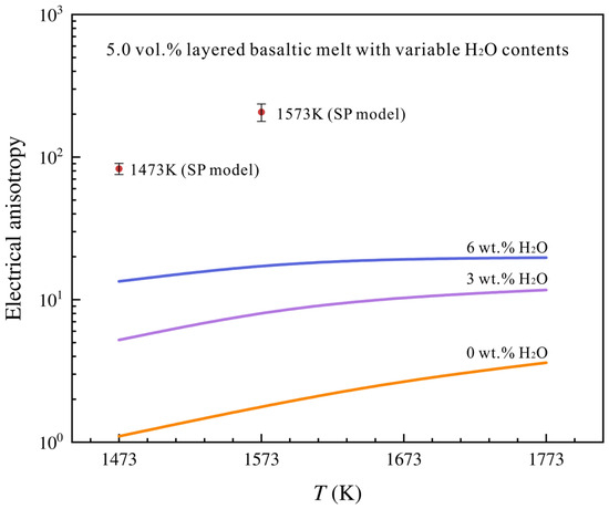
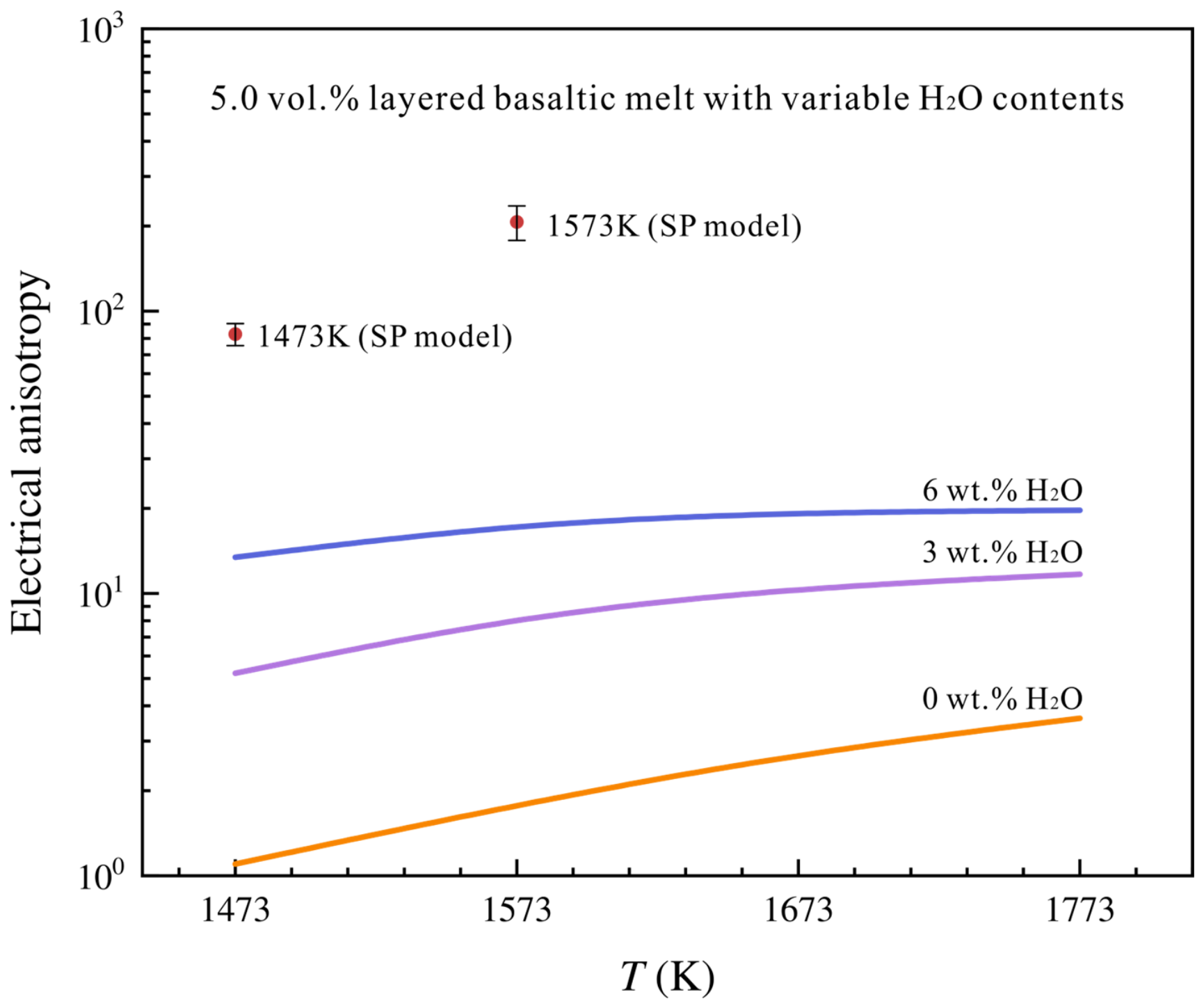
The calculated electrical anisotropy increases with both temperature and melt H2O content (Figure 6). For anhydrous basaltic melts, the calculated electrical anisotropy is close to 1 at 1473 K and gradually increases to approximately 3–4 at 1773 K. When the melt contains 3 wt.% H2O, the anisotropy is significantly higher than that of the anhydrous case, increasing from approximately 5 at 1473 K to more than 10 at 1773 K. The highest anisotropy is obtained for the model with a melt containing 6 wt.% H2O. In this case, the calculated anisotropy exceeds 10 throughout the investigated temperature range and approaches 20 at 1773 K.
Figure 6.
Electrical anisotropy of layered olivine–basaltic melt models as a function of temperature. The H2O content in the basaltic melt varies from 0 to 6 wt.% with a constant melt fraction of 5 vol.%. Solid curves represent the electrical anisotropy calculated using the GeoAnisoLab software. Red circles with error bars show the anisotropy values obtained from the series–parallel (SP) model at 1473 and 1573 K [47].
The electrical anisotropy simulated in our model is lower than that reported by Pommier et al. [47] for a similar olivine–basaltic melt layered model. This inconsistency mainly arises from the differences in the modeling approaches and conductivity data. Pommier et al. [47] used an idealized series-parallel model that did not incorporate the crystallographic preferred orientations. In contrast, the GeoAnisoLab software calculates the electrical anisotropy using the resistor network model that permits the microstructures of the olivine matrix to be incorporated. Differences in olivine conductivity data can affect the conductivity contrast between the melt-free and melt-bearing layers, thereby contributing to the discrepancy between our results and those of Pommier et al. [47]. In short, this example illustrates how the GeoAnisoLab software can be used to quantify the contribution of aligned melts to rock electrical anisotropy and further constrain the melt abundances required to match the geophysical observations.
4. Implications for Geophysical Interpretation
The GeoAnisoLab software provides a quantitative framework for linking rock-scale electrical anisotropy to geophysical observations. By providing an interactive and reproducible platform, GeoAnisoLab helps bridge mineral-physics constraints and MT interpretations. Magnetotelluric studies have detected multiple anisotropic conductivity structures in the continental crust, upper mantle, and lithosphere-asthenosphere boundary [1,2,3], but their geophysical interpretations are commonly non-unique. The GeoAnisoLab software helps address this problem by calculating the electrical anisotropy simulated for candidate rock models and testing whether these mechanisms can reproduce the magnitude of anisotropy inferred from geophysical observations.
The GeoAnisoLab software can be used for forward modeling of rock-scale electrical anisotropy. For a given region, independent constraints on temperature and geological setting can be used to construct plausible rock models. The electrical anisotropy calculated from these models can then be compared with the magnitude inferred from geophysical observations. Randomly distributed mineral aggregates can be used to evaluate the effects of mineral conductivity, crystallographic preferred orientation, and mineralogical proportions. Lithologically layered models are appropriate for regions where geological or petrological evidence supports the presence of compositional layering. If these solid-rock models produce electrical anisotropy smaller than that inferred from geophysical observations, the fluid- or melt-bearing layered models can be tested by varying the fluid/melt compositions and volume fractions. Conversely, if the solid-state rock models can reproduce the observed anisotropy, conductive fluids or melts may not be required. In comparison of the calculated and observed anisotropic results can widespread applied to constrain the ranges of fluid or melt fraction. As a result, the GeoAnisoLab software can provide a unique geophysical viewpoint for the material composition and electric transport behavior of the Earth’s deep interior.
5. Conclusions
In this study, we designed and developed the GeoAnisoLab software, which, for the absolutely new program, can be used to quantitatively evaluate the electrical anisotropy of rock by the resistor network-based circuit simulations. The GeoAnisoLab program integrates available mineralogical conductivity data, crystallographic orientation, mineralogical proportion, lithological layering, and conductive fluid/melt phase within a single computational framework. It allows users to construct different rock models, calculate their electrical anisotropy, and visualize the corresponding resistor networks. Several representative calculations display how the GeoAnisoLab software can be applied to quantify the electrical anisotropy produced by five typical petrological models (i.e., the randomly distributed rock model, two lithologically layered models, the fluid-bearing layered model, and the melt-bearing layered model). Overall, GeoAnisoLab provides an accessible forward-modeling tool for linking mineral-physics data with MT-based interpretations of anisotropic conductivity anomalies. It helps evaluate which mechanisms, including mineral fabrics, lithologic layering, and aligned fluids or melts, can account for electrical anisotropy observed in the Earth’s interior.
Author Contributions
Conceptualization: H.H. and L.D.; Data curation: S.L.; Formal analysis: S.L. and H.H.; Funding acquisition: H.H., L.D. and W.S.; Investigation: S.L.; Methodology: S.L.; Software: S.L.; Project Administration: H.H., L.D. and W.S.; Writing—original draft: S.L.; Writing—review & editing: H.H. and L.D. All authors have read and agreed to the published version of the manuscript.
Funding
This study was financially supported by the National Natural Science Foundation of China (Grant No. 42274137), Guizhou Normal University Academic New Talent Fund (Grants No. GZNUD [2025] 10 and GZNUD [2025] 12), and Guizhou Provincial Science and Technology Projects (QKHJC-ZD [2026]149 and QKHJC-ZK [2022]YB567).
Data Availability Statement
GeoAnisoLab version 1.0, together with representative results generated in this study, is openly available at [https://doi.org/10.5281/zenodo.20790196] (accessed on 11 July 2026).
Acknowledgments
We thank the editor of Leonid Dubrovinsky for kindly handling our paper, as well as the two anonymous reviewers for their constructive and enlightened advice during the revision process.
Conflicts of Interest
The authors declare no conflicts of interest relevant to this study.
References
- Heinson, G.; White, A. Electrical resistivity of the northern Australian lithosphere: Crustal anisotropy or mantle heterogeneity? Earth Planet. Sci. Lett. 2005, 232, 157–170. [Google Scholar] [CrossRef] [Scilit]
- Le Pape, F.; Jones, A.G.; Vozar, J.; Wei, W.B. Penetration of crustal melt beyond the Kunlun Fault into northern Tibet. Nat. Geosci. 2012, 5, 330–335. [Google Scholar] [CrossRef] [Scilit]
- Liu, Y.; Junge, A.; Yang, B.; Löwer, A.; Cembrowski, M.; Xu, Y.X. Electrically anisotropic crust from three-dimensional magnetotelluric modeling in the Western Junggar, NW China. J. Geophys. Res. Solid Earth 2019, 124, 9474–9494. [Google Scholar] [CrossRef] [Scilit]
- Simpson, F.; Tommasi, A. Hydrogen diffusivity and electrical anisotropy of a peridotite mantle. Geophys. J. Int. 2005, 160, 1092–1102. [Google Scholar] [CrossRef] [Scilit]
- Wannamaker, P.E. Anisotropy versus heterogeneity in continental solid Earth electromagnetic studies: Fundamental response characteristics and implications for physicochemical state. Surv. Geophys. 2005, 26, 733–765. [Google Scholar] [CrossRef] [Scilit]
- Marti, A. The role of electrical anisotropy in magnetotelluric responses: From modelling and dimensionality analysis to inversion and interpretation. Surv. Geophys. 2013, 35, 179–218. [Google Scholar] [CrossRef] [Scilit]
- Dai, L.D.; Sun, W.Q.; Li, H.P.; Hu, H.Y.; Wu, L.; Jiang, J.J. Effect of chemical composition on the electrical conductivity of gneiss at high temperatures and pressures. Solid Earth 2018, 9, 233–245. [Google Scholar] [CrossRef] [Scilit]
- Wang, D.J.; Li, H.P.; Yi, L.; Matsuzaki, T.; Yoshino, T. Anisotropy of synthetic quartz electrical conductivity at high pressure and temperature. J. Geophys. Res. 2010, 115, B09211. [Google Scholar] [CrossRef] [Scilit]
- Yang, X.Z. Orientation-related electrical conductivity of hydrous olivine, clinopyroxene and plagioclase and implications for the structure of the lower continental crust and uppermost mantle. Earth Planet. Sci. Lett. 2012, 317–318, 241–250. [Google Scholar] [CrossRef] [Scilit]
- Hu, H.Y.; Yin, C.Y.; Dai, L.D.; Lai, J.H.; Chen, Y.Q.; Wang, P.F.; Zhu, J.L.; Han, S.B. The Role of α−β Quartz Transition in Fluid Storage in Crust From the Evidence of Electrical Conductivity. J. Geophys. Res. Solid Earth 2024, 129, e2024JB029140. [Google Scholar] [CrossRef] [Scilit]
- Luo, S.; Hu, H.Y.; Dai, L.D. Electrical anisotropy calculation of the continental crust by resistor network-based circuit simulations. Appl. Comput. Geosci. 2025, 27, 100265. [Google Scholar] [CrossRef] [Scilit]
- Hashin, Z.; Shtrikman, S. A variational approach to the theory of the effective magnetic permeability of multiphase materials. J. Appl. Phys. 1962, 33, 3125–3131. [Google Scholar] [CrossRef] [Scilit]
- Schulgasser, K. Relationship between single-crystal and polycrystal electrical conductivity. J. Appl. Phys. 1976, 47, 1880–1886. [Google Scholar] [CrossRef] [Scilit]
- Shankland, T.J.; Duba, A.G. Standard electrical conductivity of isotropic, homogeneous olivine in the temperature range 1200–1500 °C. Geophys. J. Int. 1990, 103, 25–31. [Google Scholar] [CrossRef] [Scilit]
- Xu, Y.S.; Shankland, T.J.; Poe, B.T. Laboratory-based electrical conductivity in the Earth’s mantle. J. Geophys. Res. 2000, 105, 27865–27875. [Google Scholar] [CrossRef] [Scilit]
- Dai, L.D.; Hu, H.Y.; Li, H.P.; Jiang, J.J.; Hui, K.S. Influence of temperature, pressure, and chemical composition on the electrical conductivity of granite. Am. Mineral. 2014, 99, 1420–1428. [Google Scholar] [CrossRef] [Scilit]
- Sun, W.Q.; Dai, L.D.; Li, H.P.; Hu, H.Y.; Liu, C.C. Effect of temperature, pressure and chemical composition on the electrical conductivity of granulite and geophysical implications. J. Mineral. Petrol. Sci. 2019, 114, 87–98. [Google Scholar] [CrossRef] [Scilit]
- Hu, H.Y.; Dai, L.D.; Sun, W.Q.; Wang, M.Q.; Jing, C.X. Constraints on fluids in the continental crust from laboratory-based electrical conductivity measurements of plagioclase. Gondwana Res. 2022, 107, 1–12. [Google Scholar] [CrossRef] [Scilit]
- Pommier, A.; Le-Trong, E. SIGMELTS: A web portal for electrical conductivity calculations in geosciences. Comput. Geosci. 2011, 37, 1450–1459. [Google Scholar] [CrossRef] [Scilit]
- Bahr, K. Percolation in the crust derived from distortion of electric fields. Geophys. Res. Lett. 2000, 27, 1049–1052. [Google Scholar] [CrossRef] [Scilit]
- Fuji-ta, K.; Seki, M.; Ichiki, M. Random network model of electrical conduction in two-phase rock. Mineral. Petrol. 2018, 112, 857–864. [Google Scholar] [CrossRef] [Scilit]
- Hu, H.Y.; Dai, L.D.; Li, H.P.; Sun, W.Q.; Li, B.S. Effect of dehydrogenation on the electrical conductivity of Fe-bearing amphibole: Implications for high conductivity anomalies in subduction zones and continental crust. Earth Planet. Sci. Lett. 2018, 498, 27–37. [Google Scholar] [CrossRef] [Scilit]
- Bunge, H.-J. Texture Analysis in Materials Science: Mathematical Methods; Butterworths: London, UK, 1982; p. 595. [Google Scholar]
- Czertowicz, T.A.; Takeshita, T.; Arai, S.; Yamamoto, T.; Ando, J.I.; Shigematsu, N.; Fujimoto, K.I. The architecture of long-lived fault zones: Insights from microstructure and quartz lattice-preferred orientations in mylonites of the Median Tectonic Line, SW Japan. Prog. Earth Planet. Sci. 2019, 6, 25. [Google Scholar] [CrossRef] [Scilit]
- Allard, M.; Ildefonse, B.; Oliot, É.; Barou, F. Plastic deformation of plagioclase in oceanic gabbro accreted at a slow-spreading ridge (Hole U1473A, Atlantis Bank, Southwest Indian Ridge). J. Geophys. Res. Solid Earth 2021, 126, e2021JB021964. [Google Scholar] [CrossRef] [Scilit]
- Yang, X.Z. Origin of high electrical conductivity in the lower continental crust: A review. Surv. Geophys. 2011, 32, 875–903. [Google Scholar] [CrossRef] [Scilit]
- Qi, C.; Zhao, Y.H.; Zimmerman, M.E.; Kim, D.; Kohlstedt, D.L. Evolution of microstructural properties in sheared iron-rich olivine. J. Geophys. Res. Solid Earth 2021, 126, e2020JB019629. [Google Scholar] [CrossRef] [Scilit]
- Du Frane, W.L.; Roberts, J.J.; Toffelmier, D.A.; Tyburczy, J.A. Anisotropy of electrical conductivity in dry olivine. Geophys. Res. Lett. 2005, 32, L24315. [Google Scholar] [CrossRef] [Scilit]
- Dai, L.D.; Karato, S.I. High and highly anisotropic electrical conductivity of the asthenosphere due to hydrogen diffusion in olivine. Earth Planet. Sci. Lett. 2014, 408, 79–86. [Google Scholar] [CrossRef] [Scilit]
- Zhao, C.C.; Yoshino, T. Electrical conductivity of mantle clinopyroxene as a function of water content and its implication on electrical structure of uppermost mantle. Earth Planet. Sci. Lett. 2016, 447, 1–9. [Google Scholar] [CrossRef] [Scilit]
- Dai, L.D.; Karato, S.I. Electrical conductivity of orthopyroxene: Implications for the water content of the asthenosphere. Proc. Jpn. Acad. Ser. B 2009, 85, 466–475. [Google Scholar] [CrossRef] [Scilit]
- Guo, H.H.; Keppler, H. Electrical conductivity of NaCl-bearing aqueous fluids to 900 °C and 5 GPa. J. Geophys. Res. Solid Earth 2019, 124, 1397–1411. [Google Scholar] [CrossRef] [Scilit]
- Guo, X.; Zhang, L.; Su, X.; Mao, Z.; Gao, X.Y.; Yang, X.Z.; Ni, H.W. Melting Inside the Tibetan Crust? Constraint From Electrical Conductivity of Peraluminous Granitic Melt. Geophys. Res. Lett. 2018, 45, 3906–3913. [Google Scholar] [CrossRef] [Scilit]
- Ni, H.W.; Keppler, H.; Behrens, H. Electrical conductivity of hydrous basaltic melts: Implications for partial melting in the upper mantle. Contrib. Mineral. Petrol. 2011, 162, 637–650. [Google Scholar] [CrossRef] [Scilit]
- Gaillard, F.; Malki, M.; Iacono-Marziano, G.; Pichavant, M.; Scaillet, B. Carbonatite Melts and Electrical Conductivity in the Asthenosphere. Science 2008, 322, 1363–1365. [Google Scholar] [CrossRef] [Scilit] [PubMed]
- Sinmyo, R.; Keppler, H. Electrical conductivity of NaCl-bearing aqueous fluids to 600 °C and 1 GPa. Contrib. Mineral. Petrol. 2017, 172, 4. [Google Scholar]
- Mainprice, D.; Hielscher, R.; Schaeben, H. Calculating anisotropic physical properties from texture data using the MTEX open-source package. Geol. Soc. Lond. Spec. Publ. 2011, 360, 175–192. [Google Scholar] [CrossRef] [Scilit]
- Hou, C.R.; Liu, J.L.; Zhou, B.J.; Ji, L.; Fan, W.K.; Chen, X.Y.; Zhang, J. Fluid-enhanced diffusive mass transfer combined with GBS as an important process for protracted weakening in the middle-lower crust. J. Struct. Geol. 2023, 171, 104861. [Google Scholar] [CrossRef] [Scilit]
- Montanini, A.; Harlov, D. Petrology and mineralogy of granulite-facies mafic xenoliths (Sardinia, Italy): Evidence for KCl metasomatism in the lower crust. Lithos 2006, 92, 588–608. [Google Scholar] [CrossRef] [Scilit]
- Yang, X.Z.; Deloule, E.; Xia, Q.K.; Fan, Q.C.; Feng, M. Water contrast between Precambrian and Phanerozoic continental lower crust in eastern China. J. Geophys. Res. 2008, 113, B08207. [Google Scholar] [CrossRef] [Scilit]
- Yang, X.Z.; McCammon, C. Fe3+-rich augite and high electrical conductivity in the deep lithosphere. Geology 2012, 40, 131–134. [Google Scholar] [CrossRef] [Scilit]
- Huang, Y.S.; Nakatani, T.; Nakamura, M.; McCammon, C.; Yoshino, T. Electrical conductivity in texturally equilibrated fluid-bearing forsterite aggregates at high temperatures and pressures. J. Geophys. Res. Solid Earth 2021, 126, e2020JB021343. [Google Scholar] [CrossRef] [Scilit]
- Brasse, H.; Kapinos, G.; Li, Y.G.; Muetschard, L.; Soyer, W.; Eydam, D. Structural electrical anisotropy in the crust at the south-central Chilean continental margin as inferred from geomagnetic transfer functions. Phys. Earth Planet. Inter. 2009, 173, 7–16. [Google Scholar] [CrossRef] [Scilit]
- Wei, W.B.; Unsworth, M.; Jones, A.; Booker, J.; Tan, H.D.; Nelson, D.; Chen, L.S.; Li, S.H.; Solon, K.; Bedrosian, P.; et al. Detection of widespread fluids in the Tibetan crust by magnetotelluric studies. Science 2001, 292, 716–719. [Google Scholar] [CrossRef] [Scilit] [PubMed]
- Hacker, B.R.; Ritzwoller, M.H.; Xie, J. Partially melted, mica-bearing crust in central Tibet. Tectonics 2014, 33, 1408–1424. [Google Scholar] [CrossRef] [Scilit]
- Le Pape, F.; Jones, A.G.; Unsworth, M.J.; Vozar, J.; Wei, W.B.; Jin, S.; Ye, G.F.; Jing, J.N.; Dong, H.; Zhang, L.T.; et al. Constraints on the evolution of crustal flow beneath northern Tibet. Geochem. Geophys. Geosyst. 2015, 16, 4237–4260. [Google Scholar] [CrossRef] [Scilit]
- Pommier, A.; Leinenweber, K.; Kohlstedt, D.L.; Qi, C.; Garnero, E.J.; Mackwell, S.J.; Tyburczy, J.A. Experimental constraints on the electrical anisotropy of the lithosphere-asthenosphere system. Nature 2015, 522, 202–206. [Google Scholar] [CrossRef] [Scilit] [PubMed]
- Zhang, B.H.; Yoshino, T.; Yamazaki, D.; Manthilake, G.; Katsura, T. Electrical conductivity anisotropy in partially molten peridotite under shear deformation. Earth Planet. Sci. Lett. 2014, 405, 98–109. [Google Scholar] [CrossRef] [Scilit]

Disclaimer/Publisher’s Note: The statements, opinions and data contained in all publications are solely those of the individual author(s) and contributor(s) and not of MDPI and/or the editor(s). MDPI and/or the editor(s) disclaim responsibility for any injury to people or property resulting from any ideas, methods, instructions or products referred to in the content. |
© 2026 by the authors. Licensee MDPI, Basel, Switzerland. This article is an open access article distributed under the terms and conditions of the Creative Commons Attribution (CC BY) license.