Article

Stochastic Inversion of Geophysical Data by Sequential Bayesian Updating Under a Non-Stationary Gaussian Process Prior


1
Department of Earth & Planetary Sciences, Stanford University, 450 Jane Stanford Way, Bldg. 320, Stanford, CA 94305, USA
2
Department of Energy Science Engineering, Stanford University, Stanford, CA 94305, USA
*
Author to whom correspondence should be addressed.
Minerals 2026, 16(7), 736; https://doi.org/10.3390/min16070736
Submission received: 15 May 2026 / Revised: 9 July 2026 / Accepted: 10 July 2026 / Published: 14 July 2026
(This article belongs to the Special Issue Feature Papers in Mineral Exploration Methods and Applications 2025)

Abstract

The acquisition of geophysical data is becoming increasingly important in the context of critical mineral exploration. Geophysical data and inversion products are essential to map many components of the critical mineral system by detecting geophysical anomalies that can be interpreted by expert geologists. However, the inversion of airborne geophysical data acquired along flightlines into subsurface petrophysical properties remains an outstanding challenge. Many inversion techniques rely either on 1D deterministic inversion or on stochastic inversion on a local scale. The outcome of our work is the stochastic inversion along flightlines of 2D panels (flightline direction vs. depth), while at the same time producing plausible spatial variation in the petrophysical properties. Our method relies on a sequential application of Bayesian inversion, where we invert a sequence of 2D panels such that the variation in petrophysical properties avoids generation of artifacts across the panel boundaries. We show that our method can be used in a practical setting in the context of mineral exploration in the Cape Smith Belt of Canada.

1. Introduction

In the drive to explore for critical minerals needed for the energy transition, many countries have been or are in pursuit of mapping the subsurface using large-spread airborne geophysics. Typically, several types of geophysical measurements are obtained, such as gravity, magnetic, and electromagnetic (EM). Data along flightlines are then interpolated to obtain a 2D (or in EM, a time-domain) map of measured magnetic, gravity, and EM. These maps are used to detect geophysical anomalies of interest; they may be used in mineral prospectivity mapping or may guide exploration companies in drilling certain targets.
In addition, the data contain information on the variation in petrophysical properties in the 3D subsurface, and when inverted, the data turn into 3D models using either deterministic or stochastic methods. In deterministic inversion, a single model is obtained by minimizing a regularized misfit between the predicted and observed data; this yields one smooth image but no assessment of the many alternative models that could explain the data equally well. Stochastic inversion instead poses the problem probabilistically and draws an ensemble of data-consistent models, so that the non-uniqueness of the solution is sampled and the uncertainty of the recovered properties is quantified, at the cost of greater computation [1,2,3,4,5,6]. This is usually done over areas of particular interest, which tend to be limited in extent. Stochastic inversion along extensive flightlines is not common. Some methods are used in the context of scientific studies of the Earth’s crust. Other methods rely on consecutive pseudo-1D or -2D inversions along flightlines [7,8,9]. These approaches are often deterministic [10]. “2.5D inversion”, or stacking the same 2D petrophysical models into 3D, is sometimes used by assuming petrophysical homogeneity perpendicular to the lines [11]. Some recent studies in large-scale potential field inversion were conducted directly on 3D voxel models with regularization [12]. Similarly, the authors in [13] attempted to invert the 3D conductivity of the contiguous US on a 70 km grid mesh from magneto-telluric (MT) data. All of the above results were obtained by minimizing the misfit between model-predicted geophysical maps and the observed data (often interpolated) with a model parameter regularization term, using gradient-based optimization. In these approaches, a well-defined large-scale 2D/3D reference (or initial model) is essential, often with weights used to control how the inverted results closely adhere to the reference model [14]. The resulting models are typically deterministic, and defining 3D reference models at large scales can be very difficult. What is lacking today are methods that can perform stochastic inversions along flightline data. While this work does not yet cover very large areas, such as entire countries, it proposes a method that can be extended to large-scale applications.
Several challenges need to be overcome to achieve this. A single-step inversion over a large area is not feasible in terms of memory and computational resources, as well as the challenge of formulating a single prior model. To address this, we will perform stochastic inversions per panel, along the direction of the flightline, making sure that panels are stitched together without creating artificial boundaries. Secondly, the spatial variability of the petrophysical properties may change dramatically over large distances due to changes in rock properties and the probable structure controlling the rock continuity. This means that the style of spatial variability of these physical properties is likely to change in their direction of continuity (e.g., azimuthal and dipping) and in their subsurface morphologies (layers, intrusions, and folding). This means that building comprehensive prior distribution models for multiple petrophysical properties required for Bayesian inversion is challenging. To address this issue, we use non-stationary Gaussian processes as prior, where the non-stationary mean and covariance function are also uncertain, i.e., have their own prior distributions. We intend to show that with these non-stationary Gaussian priors, a wide range of possible petrophysical variations can be generated. Additionally, correlation structures related to large-scale geological structures between the various petrophysical properties can be imposed. Our approach is applied to the Cape Smith Belt, which is currently under exploration for Ni-Cu-Co sulfide deposits.

2. Application Area

Our area of study is from the Cape Smith Belt (CSB) in the Nunavik region of Northern Québec, Canada. As an early Proterozoic thrust belt containing metamorphosed basaltic volcanic, mafic intrusive, and sedimentary rocks, the CSB has been widely explored for Ni-Cu-PGE magmatic sulfide deposits. We use publicly available airborne magnetic data acquired concurrently with the HeliTEM2 survey and obtained through the Geomining Information System of Québec; these data were released into the public domain by KoBold Metals [15]. The survey was conducted by Xcalibur MPH (Canada) Ltd. using a HeliTEM2 35 m-diameter-loop electromagnetic system (Xcalibur MPH (Canada) Ltd., Toronto, ON, Canada) and a CS-3 cesium-vapor magnetometer (Scintrex Ltd., Concord, ON, Canada) [15]. The data were acquired between 18 June and 24 August 2022. The survey comprised 3626.0 km of traverse lines spaced 200 m apart and 381.7 km of tie lines spaced 1450–2000 m apart, for a total of 4007.7 km (Figure 1).
Prior to inversion, the HeliTEM2 total-field magnetic data were processed following the standard airborne magnetic workflow: removal of diurnal variations using base-station records, subtraction of the International Geomagnetic Reference Field (IGRF), tie-line levelling and micro-levelling to remove residual line noise, interpolation of the levelled data onto a regular grid, and calculation of a vertical magnetic gradient to enhance near-surface magnetic units (see [15] for processing details). These steps produce the gridded magnetic-anomaly maps that are conventionally interpreted qualitatively or inverted deterministically into a single subsurface model. What such workflows do not deliver is a quantified uncertainty for the recovered petrophysical properties. The present work addresses precisely this shortcoming: rather than a single deterministic image, it produces an ensemble of data-consistent magnetic-susceptibility models from which uncertainty can be quantified.

3. Methodology

3.1. Sequential Bayesian Updating: A Review

Our approach aims to solve a larger inverse problem by the sequential inversion of smaller panels, areas, or blocks. Since the approach is Bayesian, we will review here some fundamental concepts of sequential Bayesian updating [16,17]. Consider a model parameter, y , that is informed by a sequence of data, x 1 ,   x 2 , ,   x n . In a Bayesian context, we start with a prior distribution, p y , and at step n , we can decompose the likelihood as follows:
p x 1 , x 2 , ,   x n | y = p x 1 | y p x 2 | x 1 , y p ( x n | x n 1 , y ) .
where
x n 1 = x n 1 , x n 2 , , x 1 .
Because x n 1 is treated as a set (the history of observations), the order of its elements is immaterial for the conditioning used here.
The update distribution at time n then is the posterior:
p y | x n = p n y   ~   p y   p ( x n | y ) .
Then, after obtaining new information, x n + 1 , we start anew and update
p n + 1 y = p y | x n + 1 ~   p y   p ( x n + 1 | y ) .
Essentially, we are using the p n y as the prior distribution in the next step of the Bayesian update to get the next posterior, p n + 1 y . Indeed, we can derive that the posterior of y at step n becomes the prior at step n + 1 .
p n y p x n + 1 | x n , y = p y p x n | y p x n + 1 | x n , y = p y p x n + 1 | y   ~   p n + 1 y .
Note that we do not need a conditional independence assumption in this derivation. The revised posterior equals the current posterior times the likelihood of the new data. All historical knowledge about y is captured by p n y . The sequential application of Bayes’ rule is therefore recursive.
Consider now a problem with a dynamic y , changing in time (or in space, or both), and a Markovian (conditional independence) model is used:
p y n + 1 | y n =   p y n + 1 | y n ,
where y n = y n ,   y n 1 ,   ,   y 1 .
The true state is not observed; instead, a sequence of data is acquired. Assuming conditional independence,
p x n | y n , x n 1 = p ( x n | y n ) .
Then, the joint density becomes
p x n , y n = p y 0 i = 1 n p y i | y i 1 p ( x i | y i ) .
The dynamic evolution of y is modeled using two steps: predict y at time n from data at previous times (filter step) and predict a y at the next step, n + 1 . The filter distribution is the posterior, p ( y n | x n ) . Using this filter distribution, the predictive distribution becomes
p y n + 1 | x n = y n p y n + 1 | y n   p ( y n | x n )   d y n .
After a new observation, x n + 1 , is obtained, application of recursive Bayes combines the predictive distribution with a new likelihood, p ( x n + 1 | y n + 1 ) :
p y n + 1 | x n + 1 = p y n + 1 | x n + 1 ,   x n = p y n + 1 | x n   p ( x n + 1 | y n + 1 ) .
where now x n + 1 is conditionally independent of x n , knowing y n + 1 . This formulation looks deceptively simple because calculating high-dimensional pdfs and dealing with non-linear dynamics require Monte Carlo simulations. Common approaches are the use of sequential Monte Carlo methods such as particle filtering [18]. However, we will show in the next section that such methods become difficult to apply in a large-scale spatial context, where the model and data are both high-dimensional, and the physical model is CPU demanding.

3.2. A Bayesian Formulation for Large-Scale Geophysical Inversion

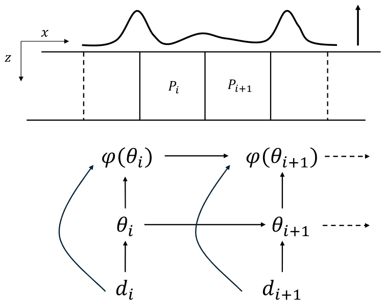
To model large areas, we divide the area over which data need to be inverted into blocks (3D), or, here, into 2D panels (in x and z direction); see Figure 2. For each block, we assume the prior to be a Gaussian process but with unknown covariance and mean function [19,20]. Let φ be a stationary Gaussian process, and then for each panel, P i , we have
φ i = φ s ,   s   ϵ   P i .
A stationary Gaussian process is fully defined by stationary mean and covariance:
E [ φ ( s ) ] = μ C o v φ s i , φ s j = E φ s i μ φ ( s j ) μ = C s i s j ,
where C is any positive definite function, and where the random vector of any set of spatial locations, s1, …, sn is
φ = φ s 1 , φ s 2 , , φ s n ,
and is multivariate Gaussian:
φ ~ 1 2 π n / 2 Σ 1 / 2 exp 1 2 φ μ T Σ 1 φ μ , Σ i j = C s i s j .
If we consider the mean and covariance function to be the (hyper)-parameters, θ , of the stationary process, then we can introduce the notation φ i θ i .
Figure 2 shows the sequential Bayesian model that applies to this case. In comparison with the notation of the previous section, we have y = φ , θ and the x   =   d , the geophysical data. The difficulty in applying the sequential approach to our problem is that
  • φ  represents a process in space and is high-dimensional;
  • θ  that defines the process φ  is unknown;
  • The relationship between θ  and  d  is not known/intractable;
  • The relationship between φ  and  d  is known but not linear;
  • Spatial dependency exists between φ n and φ n + 1 , as well as θ n and θ n + 1 .
Still, we can apply the “predict plus filter” approach to this problem:
  • Predict: Sample the posterior distribution of the next panel, P i + 1 , given the previous panel, P i . This will require enforcing spatial correlation between φ n and φ n + 1 , as well as θ n and θ n + 1 .
  • Filter: Sample the posterior distribution of the next panel, given the geophysical data of the next panel. This requires solving an inverse problem using the geophysical data of the next panel and the predictive distribution as the prior distribution (relying on the recursive Bayes model).
Consider the first panel, P 0 . In the first step, using the (stated) prior distribution,
p θ 0 , φ 0 = p θ 0   p ( φ 0 | θ 0 ) ,
we sample several realizations of θ 0 and then of φ 0 , creating realizations θ 0 , φ 0 i ,   i = 1 , , L . In the next step, we need to filter the geophysical data, d 0 ; in other words, we need to solve an inverse problem. Solving such a problem requires sampling from p ( θ 0 , φ 0 | d 0 ) . This problem is treated in Section 3.3. After inversion, the next set of particles, θ 1 , φ 1 i , needs to be predicted from the updated set, θ 0 , φ 0 i . The relationship between φ 1 and φ 0 is linear, since they model the same property. In geostatistical jargon, any realization of φ 0 serves as hard/exact data for constraining the Gaussian process, φ 1 . At the same time, we need to sample θ 1 , given θ 0 . This problem is treated in Section 3.4. Then, this procedure is recursively applied until all panels have been inverted.
Our approach will use Monte Carlo simulation, but it does not employ particle filtering, meaning that we sample directly from the posterior distribution without employing an importance sampler. Instead, we leverage high-performance computing to generate an ensemble of inverted models, computed in parallel. Next, we will detail both the filter and predict step.

3.3. Filter: Inversion of a Single Panel

We now focus on the filtering aspect of our sampler. θ and φ   need to be inverted (filtered) sequentially, honoring the hierarchical relationship between them. To do so, we propose the following decomposition of the joint inversion of θ and φ at step n :
p θ n , φ n | d n = p θ n | d n   p φ n | d n , θ n .
Consider first p θ | d , whose dimension is low. For example, in 2D, the Gaussian process has a maximum of three parameters for the covariance function (one angle and two ranges), and a mean and variance, giving a total of five parameters. This suggests modeling p θ | d as a high-dimensional density function. To estimate this density function, we generate a training set by the Monte Carlo simulation, then estimate p θ | d , and then sample from the estimated distribution with an exact method. More specifically, consider the joint distribution:
p θ n , d n = p θ n ) p ( d n | θ n = p θ n p d n | φ n p ( φ n | θ n ) ,
using the Bayes’ network definition (Figure 2) in the last step, where d n is related to θ n , through the spatial model, φ n . To sample a joint distribution, p θ , d , for any panel ( n ) (in Equations (18)–(22), the panel subscript, n, is dropped for brevity), we therefore perform the following sequential sampling:
θ j ~   p θ ,
Then, we sample a Gaussian process realization:
φ j ~ p ( φ | θ j ) ,
And then, we forward-model the data:
d j = g φ j .
Note that we use a superscript, j , to indicate a sample, while using a subscript to indicate a panel. We now have the training dataset:
θ j , d j ,   j = 1 , , J .
The training set is used to fit a high-dimensional probability density model, p ^ θ , d , from which a conditional distribution can be calculated:
p ^ θ | d = p ^ θ , d p ^ d .
For the second term, p φ | θ , d , we need to solve a non-linear inverse problem with a Gaussian prior whose hyperparameters are known. In Appendix A, we review two known solutions for this problem through the gradual deformation method (GDM) and the probability perturbation method (PPM) [21,22,23,24]. These methods were implemented using the fast Fourier transform for Gaussian process simulation with GeoStats.jl version 0.75.0 under Julia version 1.10.5 [19,20,25].

3.4. Predict: Generating a New Prior

At this stage, we need a predictive distribution that generates a new prior for the next inversion. Practically speaking, we have a set of realizations of the previous panel that match the geophysical data of that panel. Following Equation (15) of the predictive model, we need to specify p φ n + 1 , θ n + 1 | φ n , θ n , which can be further decomposed as
p φ n + 1 , θ n + 1 | φ n , θ n = p φ n + 1 | φ n , θ n , θ n + 1   p θ n + 1 | φ n , θ n .
The first term is the distribution of a Gaussian process conditioned to a previously sampled Gaussian process in panel P n , with known covariance parameters. This is a solved problem in geostatistics known as conditional simulation under a Gaussian model, for which several sampling algorithms are available, such as sequential Gaussian simulation [19,20,25].
In the second term, we need to impose spatial continuity between the hyperparameters. First, we assume conditional independence:
p ( θ n + 1 | θ n , φ n ) p ( θ n + 1 | θ n ) ,
To determine p ( θ n + 1 | θ i ) , we consider that θ n + 1 depends on θ n , because the data, d n + 1 , is correlated to d n . In Section 3.3, we saw how we can estimate both p θ n | d n and p ( θ n + 1 | d n + 1 ) . We therefore approximate p ( θ i + 1 | θ i ) using a distribution p * ( θ i + 1 | θ i ) estimated from samples θ i *   and   θ i + 1 * as follows:
p ( θ i + 1 | θ i ) p * ( θ i + 1 | θ i )   with   θ i * ~ p θ i | d i   a n d   θ i + 1 * ~ p θ i + 1 | d i + 1 .

3.5. Complete Methodology

Our method is a Monte Carlo method, meaning that each spatial model that matches all the geophysical data is sampled independently. We do not employ a particle filter where an ensemble model is updated jointly. As outlined in the previous section, there are methodological challenges that make application of particle filtering challenging. Additionally, by leveraging parallel computing, we can run each sample on a different GPU/CPU. With 100 cores, the cost of 100 samples is the same as for one sample. A naïve Monte Carlo method is also much more straightforward to implement compared to a particle filter, which requires the additional modeling of an importance sampler, which is not trivial when dealing with spatial models.
Algorithm 1 summarizes, using the above notations, the two main steps of the process, which are as follows:
  • Estimating a predictive model for the hyperparameters of the Gaussian process;
  • Iterative application of the filter and predict steps.
Algorithm 1. For the proposed algorithm, p ^   and   p * are estimated within the algorithm steps.
InputPrior p θ 0 ,   p φ 0 θ 0 .
Geophysical data per panel:   d o b s , 0 ,   d o b s , 1 ,   ,   d o b s , n .
OutputPosterior samples φ 0 , p o s t ,   θ 0 , p o s t ,   φ 1 , p o s t ,   θ 1 , p o s t ,   ,   φ n , p o s t ,   θ n , p o s t .
Estimate a predictive model for Gaussian process hyperparameters (training set):
Sample:   θ j   ~   p θ 0 ;   φ j   ~   p φ 0 θ 0 ,   j = 1 , ,   J .
Calculate: d ( j ) = g θ j ,   j = 1 , , J .
Estimate:   p ^ ( θ | d )   ( Equation   ( 22 ) )   using   samples   ( θ j , d ( j ) ) ,   j = 1 , , J .
Sample   θ 0 * , ( j ) ~ p θ 0 d 0   a n d   θ 1 * , ( j ) ~ p θ 1 d 1 ,   j = 1 , , J .
Estimate:   p * ( θ 1 | θ 0 )   ( Equation   ( 25 ) )   using   samples   ( θ 0 * , ( j ) , θ 1 * , ( j ) ) ,   j = 1 , , J .
Do Panel 0:
Predict:   θ 0 , o b s   ~   p ^ θ d o b s , 0 ;   φ 0 , o b s   ~   p φ 0 θ 0 .
Filter:   φ 0 , p o s t   ~   p φ 0 d o b s , 0 , θ 0 , o b s using GDM or PPM
F o r   P a n e l   i = 1 , ,   n
Predict   θ i , o b s *   ~   p * θ i θ i 1 ;   φ i , o b s   ~   p φ i φ i 1 , θ i .
Filter:   φ i , p o s t   ~   p φ i d o b s , i , θ i , o b s using GDM or PPM.
EndRepeat starting with Panel 0.

4. Application

4.1. Illustration of a Two-Panel Case

4.1.1. Falsification Test for the Prior, p θ 0

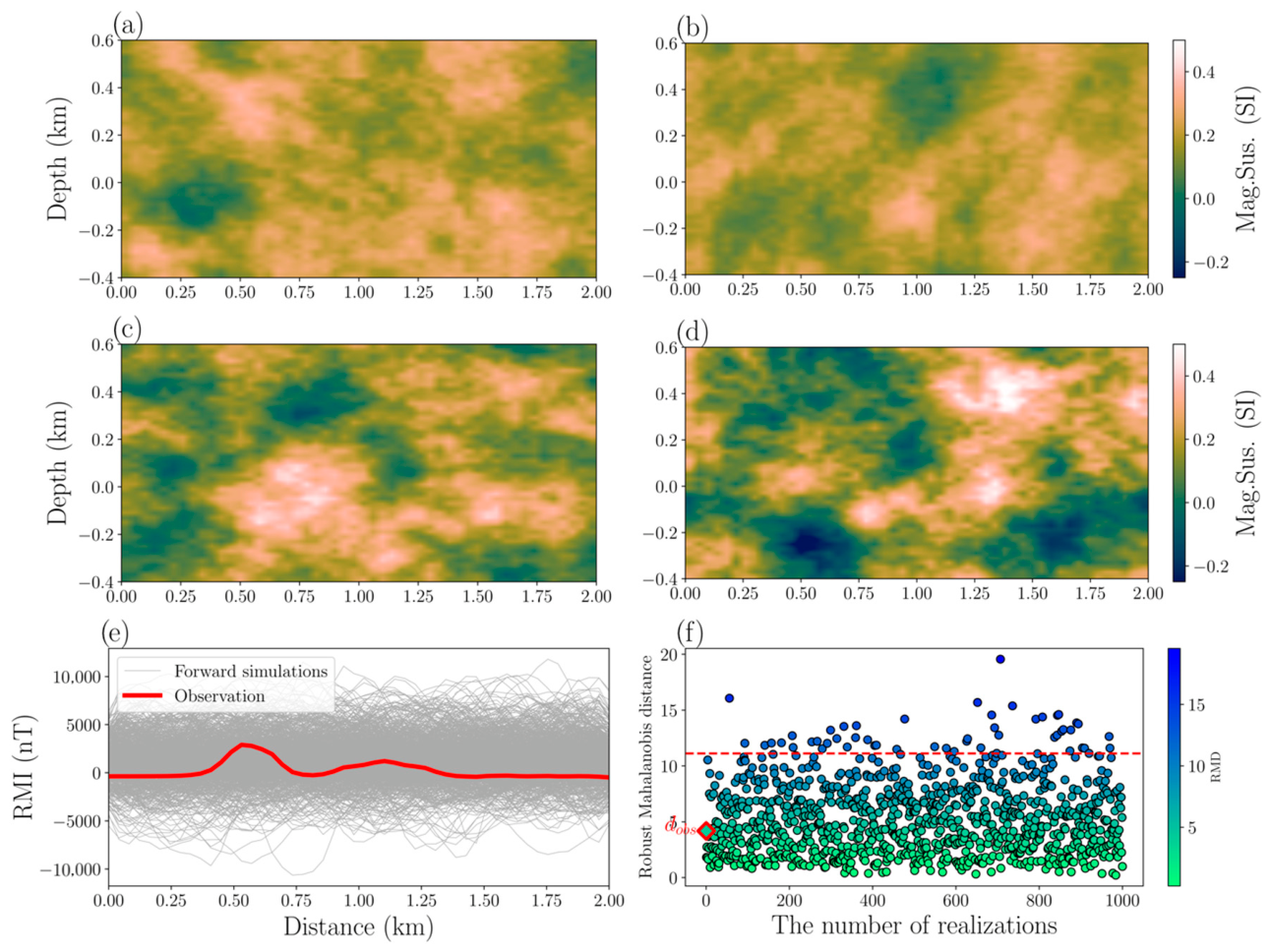
Before moving to the full real case, we present in detail the application of the above methodology to a two-panel case. Application to multiple panels is then the sequential application of the two-panel solution. Before starting the iterative filter, we need to generate a training set for predicting the conditional hyperparameter distribution, p ^ θ | d , and derive from this p * ( θ i + 1 | θ i ) . The training set should be able to predict the data along a line. In other words, a falsification test is needed on the prior distribution, p θ 0 ; see Figure 3. Such a falsification test requires sampling models from the prior, running the forward simulator and testing whether the data are an outlier with respect to the simulated data. Figure 3 shows the application of the falsification test on the two-panel case. The prior is taken to be a wide, uniform prior (Table 1). Samples of θ and φ   are sampled following the hierarchical framework, and the simulated data are generated by forward modeling. We use a Robust Mahalanobis Distance test to define whether the data are an outlier with respect to the simulated data samples. Figure 3 shows that this is not the case.

4.1.2. Estimate Predictive Models for Gaussian-Process Hyperparameters

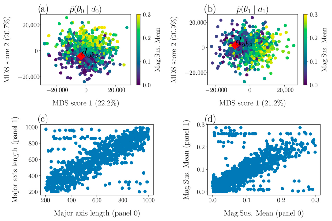
The purpose of this step is to learn, from the Monte Carlo training set, the two statistical relationships that drive the sequential scheme: (i) the conditional distribution, p ^ θ | d , which links the Gaussian-process hyperparameters, θ , to the geophysical data, d , and allows the filter step to convert an observed datum into plausible hyperparameters (Equation (22)); and (ii) the predictive distribution, p * ( θ i + 1 | θ i ) , which links the hyperparameters of one panel to those of the next and allows the predict step to propagate the prior from panel to panel (Equation (25)). Figure 4 illustrates how both are obtained.
Figure 4 shows the various steps to estimate and then sample from p * ( θ i + 1 | θ i ) . First, the data are reduced in dimension using MDS (multidimensional scaling). In this case, the first five principal components contain more than 95% of variance. The dimension of θ   is five, so a total of 10 dimensions cover the hyperparameter and data variables. Figure 4 shows a projection into 2D data (first two principal directions for d) and 1D parameter (mean). The pdfs, p ^ θ | d , are estimated using kernel density estimation. Figure 4 shows the resulting correlation between the mean and the major range. Thus, a correlation exists between the hyperparameters of two consecutive panels.

4.1.3. Predict and Filter

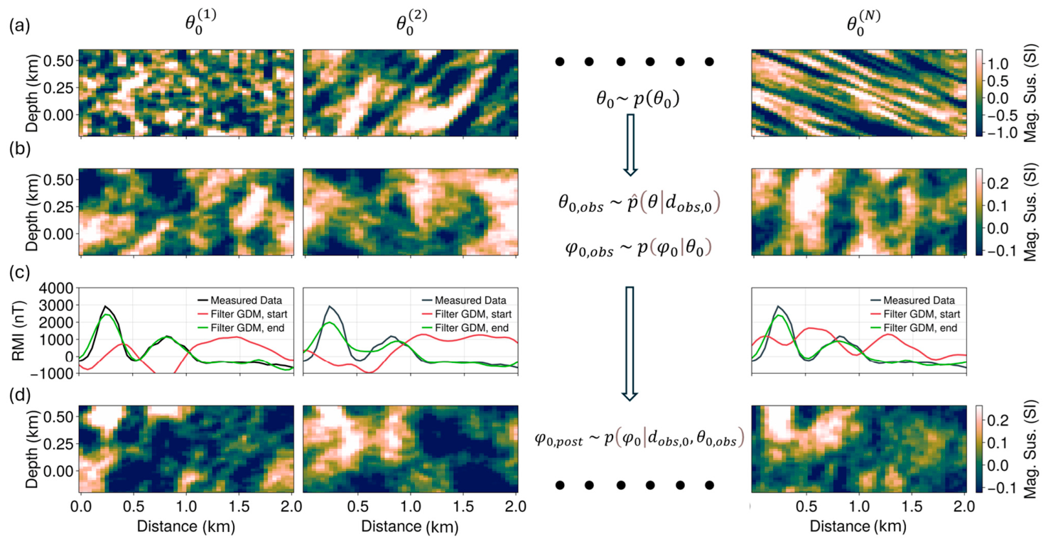
Panel P 0 needs to be inverted from the geophysical data above that panel. This requires first sampling θ 0 ~   p ^ θ 0 | d o b s , 0 and then GDM (Appendix A) on the first panel, using a Gaussian process with hyperparameters, θ 0 . Figure 5 shows three representative initial realizations (out of the full ensemble of N) sampled from the prior. The second row shows the same three realizations with hyperparameters sampled from p ^ θ 0 | d o b s , 0 . Each realization is then perturbed using the GDM method to achieve models that match the observations; see the bottom two rows in Figure 5.
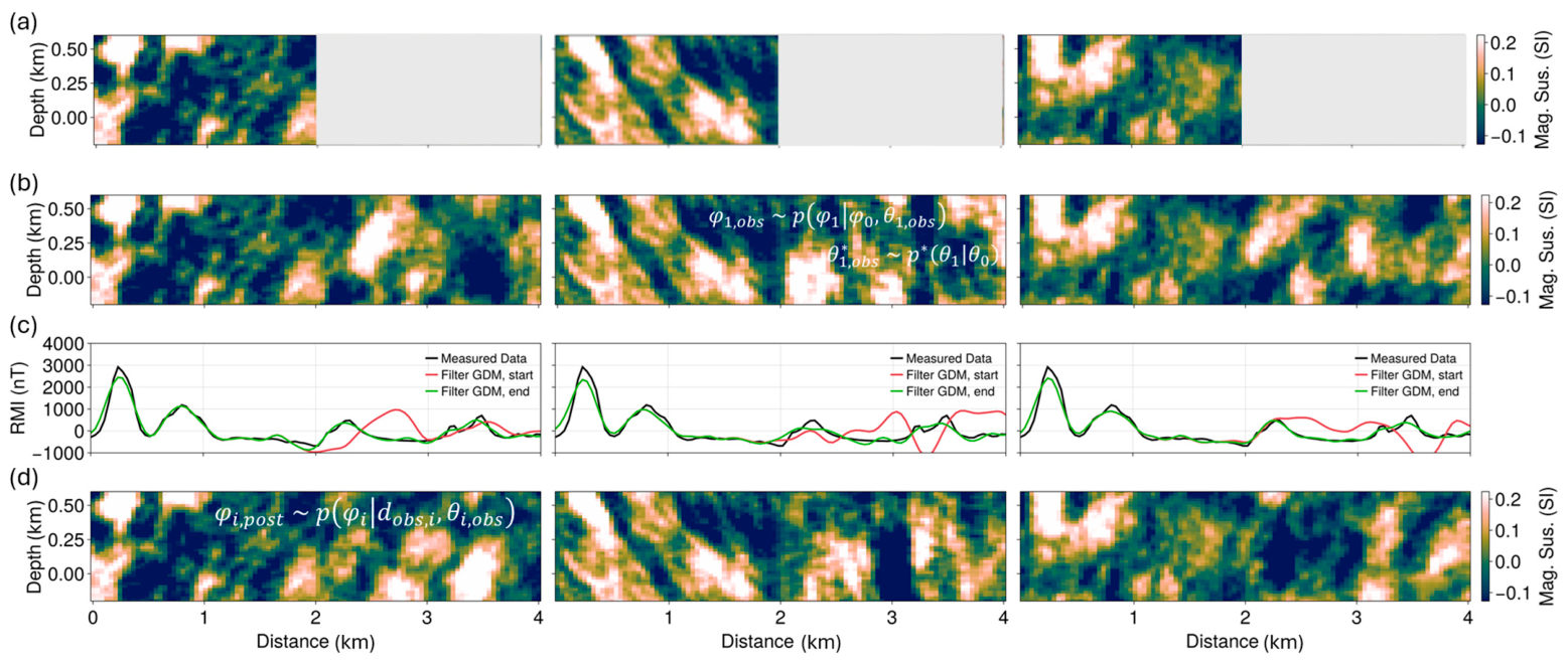
The next step is the prediction of the next panel (gray panel), P 1 ; see Figure 6. In this step, we first sample θ 1 ~ p * θ 1 | θ 0 and then sample realization of panel 1, constrained (conditioned) to the magnetic susceptibility of the previous panel. These realizations are the new predictive distribution that goes into the gradual deformation method to generate models that match the data. This procedure is iterated if more panels need to be inverted.

4.2. Four-Panel Case: Uncertainty Analysis

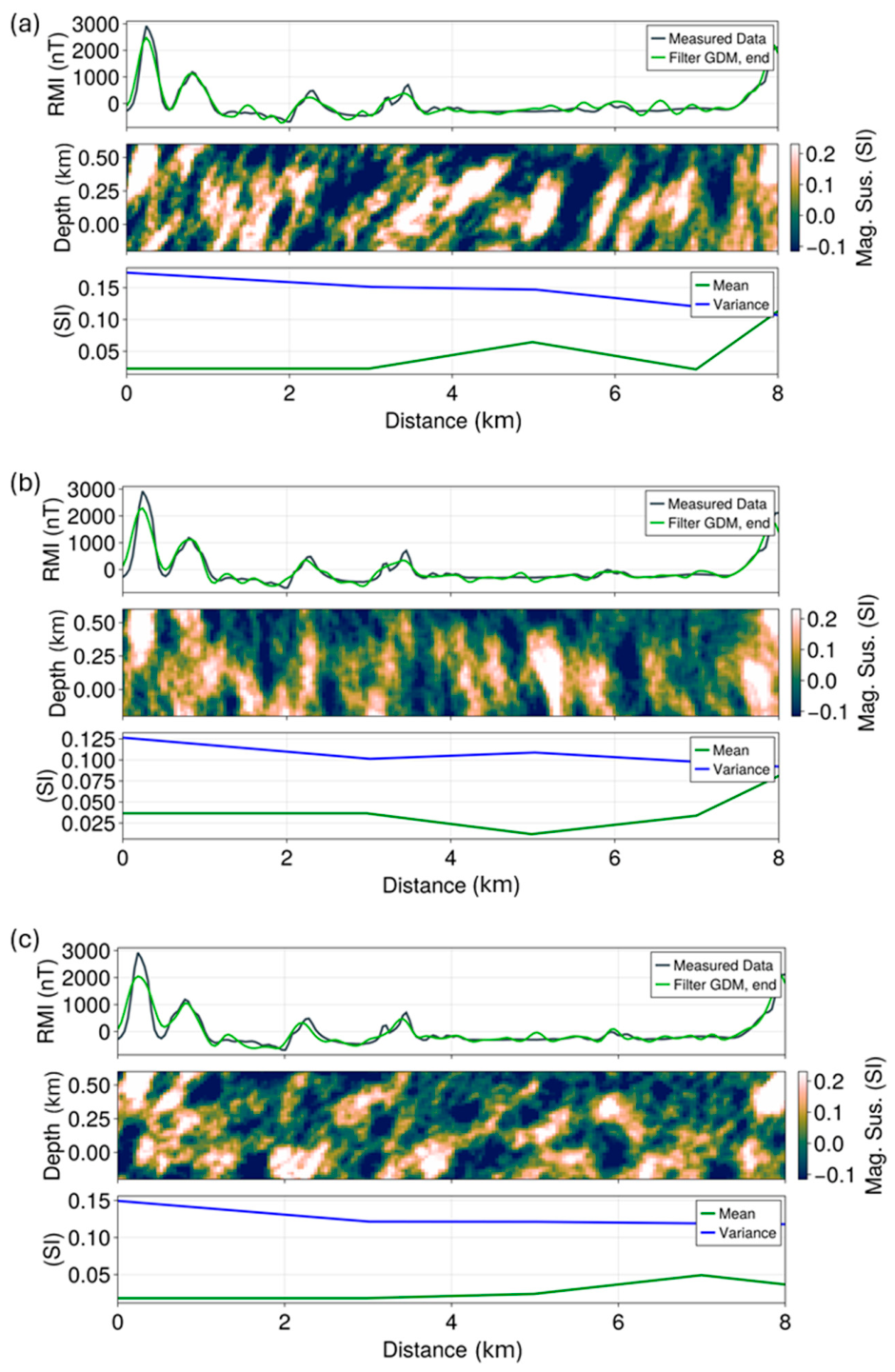
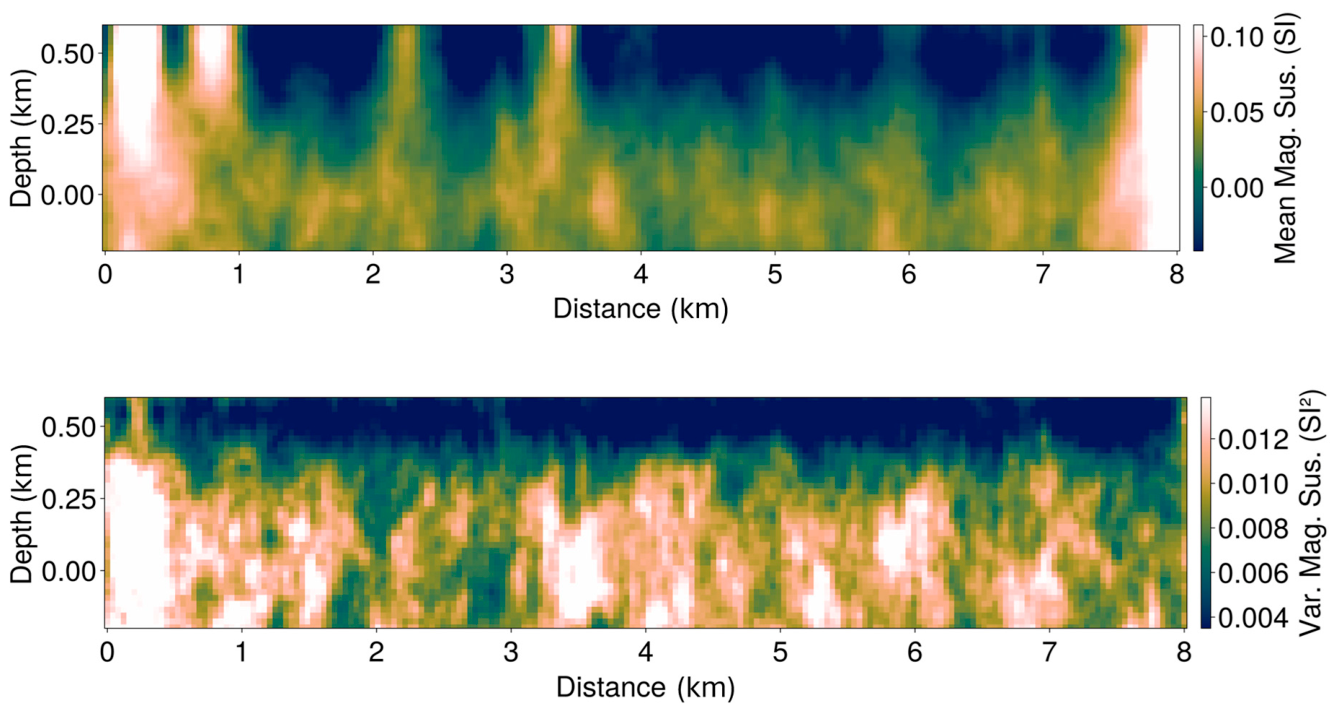
Figure 7 shows three realizations of the full four-panel case (L2 flight line; see Figure 1), together with the ensemble mean and ensemble variance. Because of the averaging, the ensemble mean loses spatial correlation that might exist and represents a smooth model (much like a deterministic inversion), as shown in Figure 8. The ensemble variance can be seen as one metric that characterizes uncertainty (but not the only one). We observe here that the variance increases with depth, but not uniformly. For example, the area in the first 1 km has much higher uncertainty (and higher mean) than the rest of the panel.

4.3. Uncertainty Quantification with Multiple Parallel Panels

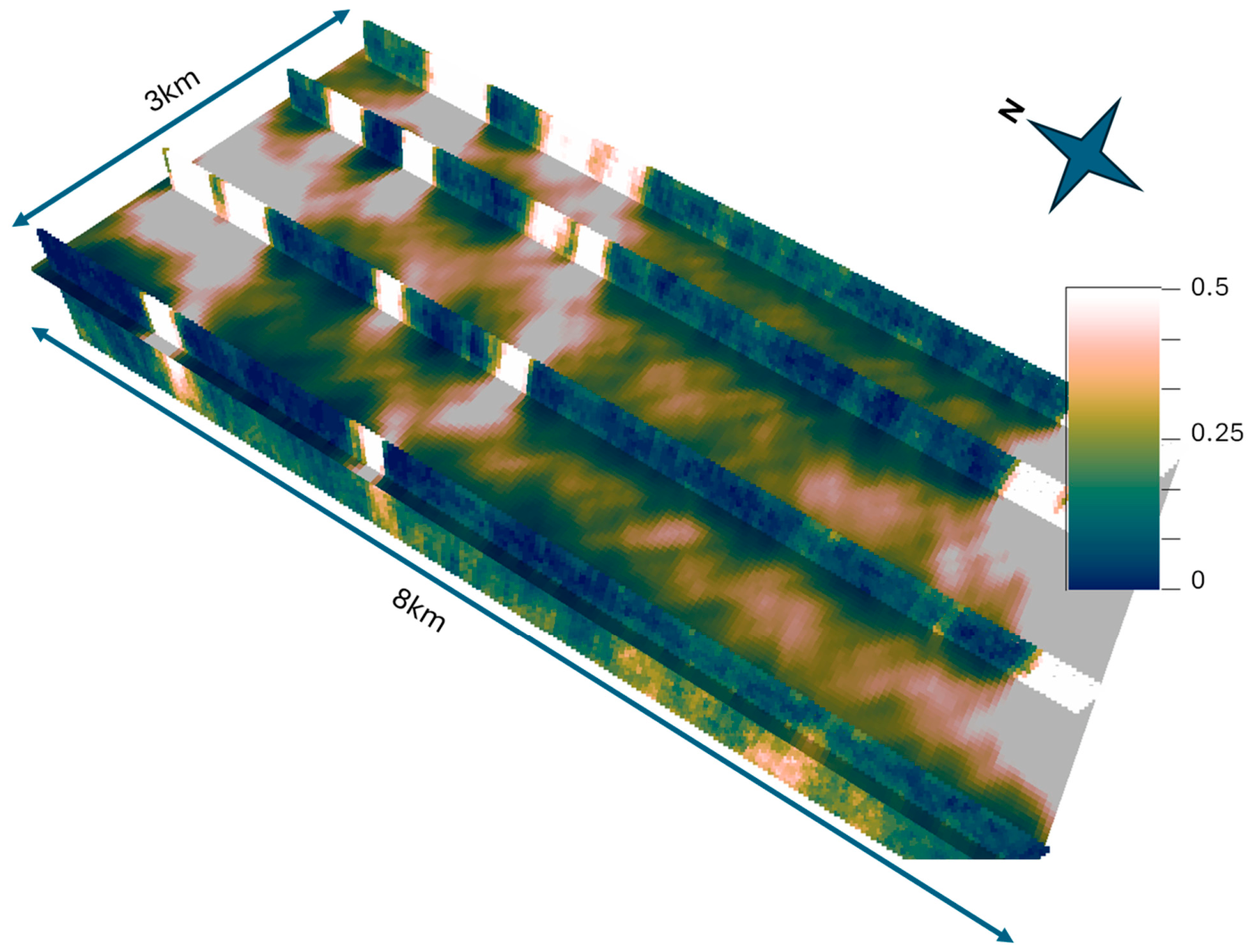
We ran the same procedure on four parallel lines (L1–L4 in Figure 1), each with four panels. Because each realization is an independent sample of the posterior, the ensemble provides, at every location, a Monte Carlo estimate of the probability that the magnetic susceptibility exceeds a given threshold. For example, in Figure 9, we plot the probability that the magnetic susceptibility is above 0.039 (which is the 75% quantile of the inverted magnetic susceptibility). High probability means high likelihood of exceeding this threshold. Regions of high probability correspond to zones likely to host elevated magnetic susceptibility within the domain. The results can be used by geologists/geophysicists for further interpretation of what these features mean and how they are to be connected in 3D.
From a geological standpoint, the elevated magnetic-susceptibility zones imaged along lines L1–L4 (Figure 1) are consistent with the mafic and ultramafic intrusive rocks that characterize the Cape Smith Belt. In this belt, the Ni-Cu-PGE magmatic sulfide mineralization is hosted by such mafic–ultramafic bodies, which commonly carry magnetite and therefore produce strong magnetic responses [27]. The high-probability susceptibility anomalies of Figure 9 can thus be interpreted as candidate mafic–ultramafic intrusions and their contacts, which are the primary exploration targets in the region. Because our approach quantifies the probability that the susceptibility exceeds a chosen threshold, it provides a probabilistic delineation of these prospective host rocks rather than a single deterministic image, helping to prioritize drilling targets while making the associated uncertainty explicit.
Figure 9. Probability for magnetic susceptibility to be above 0.039, calculated from multiple realizations and interpolated in 3D using Gaussian Process Regression [28].
Minerals 16 00736 g009

5. Discussion

Choosing a prior model for inversion is challenging, and then using such a prior model in the inversion is equally challenging. In this paper, we introduce a non-stationary Gaussian process prior model that provides compromises on both challenges. This Gaussian prior has the flexibility to match data well because the mean and covariance terms are considered uncertain, in addition to the spatial uncertainty of a petrophysical property. Gaussian models can easily be simulated in sequences of panels without artifacts, thereby making large-scale inversion possible. Additionally, many inversion algorithms exist for Gaussian priors. We used the probability perturbation method, but anyone’s favorite method can be used as well. The compromise lies in the fact that the Gaussian prior cannot capture more complex and detailed geological variability, such as faulting, stratigraphy, and other discrete features. Our procedure includes a falsification test to investigate if the Gaussian prior should be rejected, which may be the case with significant discrete changes in the data.
However, we believe it is a step forward in the context of mineral exploration, where the common practice is to first perform a deterministic smooth geophysical inversion, and then only do a manual interpretation of the results. Such a manual interpretation may however be biased because deterministic inversion may ignore important sources of variability, as we have shown through the many alternative data-matching inversions that look very different from a deterministic inversion. As a result, planning drilling based on deterministic inversion only may miss the very magnetic-susceptibility anomaly one wants to target. At a minimum, this method may help geologists interpret deterministic inversion, since now uncertainty is quantified. The latter is very useful to avoid overinterpreting detailed features of the deterministic inversion. A probability model such as shown in Figure 9 will help in avoiding such overinterpretation.
The proposed approach has a remarkably small computational footprint. The GDM iterations and panels along a flightline are computed sequentially and on a single thread. The method scales through parallelization at the level of independent realizations. Per-realization memory is in the order of 1.1 GB, so an ensemble of 100 realizations occupies approximately 110 GB of RAM and fits comfortably on a single multi-core workstation. On the AMD EPYC 7713 used for our experiments, with 64 physical cores and 128 hardware threads, the per-panel cost is dominated by the 150 GDM outer iterations needed to converge to a data-matching realization. A single realization spanning four panels completes in 45 min to 1 h, and because the 100 realizations run concurrently, the full ensemble completes in essentially the same wall-clock. The wall-clock scales linearly with the length of the flightline. Ensemble-based stochastic inversion at the line scale therefore runs on a single workstation in under an hour.
Because of its flexibility, the methodology can be extended. Importantly, the framework is agnostic to the geophysical forward operator: it only requires a forward model linking the petrophysical property to the measured response, so the same sequential Bayesian scheme applies to potential-field data (gravity and magnetic, as demonstrated here), as well as to electromagnetic data. For example, one may invert 3D blocks instead of panels and perform inversion of such blocks in a sequence such that a very large area is covered in 3D. The method can be extended to multi-physics inversion by adding a model of co-variation between two or more petrophysical properties. Several such models are available for Gaussian processes in the geostatistical literature [29,30,31].

6. Conclusions

An increase in the demand for critical minerals will necessitate the acquisition and inversion of massive amounts of geophysical data. In terms of inversion, the focus so far has mostly been on large-scale deterministic inversion, or local-scale stochastic inversion. Large-scale stochastic inversion, producing multiple models of petrophysical properties, has not yet been achieved. In this paper, we present a methodology that takes a step in that direction. Our methodology implements a sequential Bayesian inversion of blocks of data while avoiding the creation of artifacts at the block boundaries. The latter is achieved by formulating the prior distribution models as a non-stationary Gaussian process that is sequentially simulated from block to block. The filtering step is achieved by means of the probability perturbation method that inverts each block locally. Having knowledge of uncertainty may prevent overinterpreting variation in the inversion that is a risk with traditional deterministic inversion.

Author Contributions

All authors contributed to defining the problem and to the study’s conception and design. Conceptualization, J.K.C. and D.Z.Y.; methodology, J.K.C., D.Z.Y., J.P.D. and J.K.; software, J.K., J.P.D. and D.Z.Y.; validation, J.K.C., D.Z.Y., P.L., J.P.D. and J.K.; formal analysis, J.P.D., P.L., J.K. and D.Z.Y.; investigation, J.P.D., P.L., J.K. and D.Z.Y.; resources, J.K.C.; data curation, J.P.D. and P.L.; writing—original draft, J.K.C.; writing—review and editing, C.S., P.L., J.P.D., J.K. and D.Z.Y.; visualization, J.P.D., J.K., P.L., D.Z.Y. and J.K.C.; supervision, J.K.C., C.S. and D.Z.Y.; project administration, D.Z.Y.; funding acquisition, J.K.C. All authors have read and agreed to the published version of the manuscript.

Funding

This research received no external funding.

Data Availability Statement

The HeliTEM2 airborne magnetic data analyzed in this study are publicly available through the Geomining Information System of Quebec (assessment work GM 72975) at https://gq.mines.gouv.qc.ca/documents/EXAMINE/GM72975 (accessed on 9 July 2026), released to the public domain by KoBold Metals [15]. The methodology, including the sequential Bayesian framework, the gradual deformation method, and the probability perturbation method, is fully described in the manuscript and Appendix A; underlying Gaussian process simulation routines are available through the open-source GeoStats.jl package [25]. The inverted realizations generated for this study are not retained and are therefore not available for redistribution; however, they can be reproduced from the publicly available input data using the methodology described herein.

Acknowledgments

The authors gratefully acknowledge KoBold Metals for releasing the HeliTEM2 survey data into the public domain, Xcalibur Smart Mapping for the airborne data acquisition, and the Government of Québec (Geomining Information System) for hosting and curating the public dataset. The authors also acknowledge the Stanford Intelligent Systems Lab (SISL) for providing the computational resources used in this study. We also would like to acknowledge the affiliate members of Stanford Mineral-X for supporting this research, including KoBold Metals, Birdra, Ero Copper, Fleet Space Technologies, Ideon Technologies, Xcalibur, and Edra Labs.

Conflicts of Interest

The authors declare no conflicts of interest.

Appendix A. Solving a Non-Linear Inverse Problem Using a Gaussian Prior

Appendix A.1. Generating Correlated Samples from a Univariate Distribution

Solving inverse problems that involve spatial models is challenging because of the high dimensionality of the model and the difficulty of creating perturbation mechanisms consistent with a prior distribution. For example, in an McMC sampler of the posterior, one would need to design a proposal distribution that (1) generates a proposal spatial model and (2) respects the spatial correlation imposed in such a spatial model. In the case of a Gaussian process prior, this means that any perturbation of the model still needs to be a sample of those same Gaussian priors. Several methodologies have been proposed (see Chapter 6, [16]). In our work, we will use the gradual deformation method (GDM) and probability perturbation method (PPM) [21,22,23,24].
To present these methods, we consider first a simple example, namely that of sampling from the exponential distribution
u = F x = P X x = 1 exp   λ x .
The quantile function is known analytically:
x = Q u = 1 λ l o g 1 u .
Hence, exact sampling is possible. Naïve Monte Carlo generates independent draws from this distribution. Let us now consider a sampling scheme where draws are no longer independent, but with serial correlation, yet still are samples of the same exponential distribution. In an independent draw, we sample two independent values, u 1 and u 2 , and then evaluate the quantile function. Now, we would like u 2   to be a small perturbation of u 1 ; hence, x 1 is a small perturbation of x 2 . To do this, we need to be able to generate correlated draws from the uniform distribution. We first consider a standard Gaussian distribution and make correlated draws from that distribution, and then perform a rank-preserving transformation of the Gaussian draws into draws, u . We do it this way because there is a simple way to generate correlated Gaussian draws. Namely, consider a standard Gaussian draw, y 1 , then draw a second, independent draw, y 2 , and calculate the following value:
y r = y 1 cos r + y 2 sin r ,
When r = 0 , then y r = y 1 and when r = π / 2 , y r = y 1 . Also, no matter what value r has, y r is always standard Gaussian, namely
E Y r = c o s r E Y 1 + s i n r E Y 2 = 0 , V a r Y r = E Y r 0 2 = cos 2 r v a r Y 1 + sin 2 r v a r Y 2 = 1 .
Therefore, Y r represents a gradual perturbation between two independent draws, y 1 and y 2 . The gradual deformation algorithm iterates these perturbations between different Gaussian draws each time these Gaussian draws can be transformed into uniform draws using the Gaussian quantile function:
u r = G y r ~ U n i f o r m 0 , 1 .
Algorithm A1. Gradual deformation method
Input: u 0   ~   U n i f o r m 0 , 1 ; Δ r ; λ = mean of the exponential distribution.
Output: Correlated draws of P X x = 1 exp λ x
   f o r   i = 1 , , N
u i   ~   U n i f o r m 0 , 1
y i = G 1 u i
f o r   r = π , π with steps Δ r
   y r = y i 1 cos r + y i sin r
   u = G y r
   r e t u r n :   x = 1 / λ   l o g 1 u
end
end
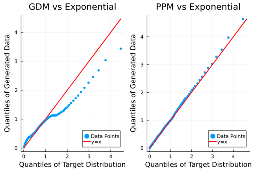
In Figure A1, we compare the gradual deformation samples of the exponential distribution with the naïve Monte Carlo. The QQ plot shows however some deviation from the exponential distribution. This issue was discussed in [24] and attributed to the fact that successive linear combinations eventually lead to a deviation from the target Gaussian (or uniform distribution).
Figure A1. Comparing naïve Monte Carlo with sampling of the exponential distribution based on the gradual deformation method (left) and the probability perturbation method (right).
Minerals 16 00736 g0a1
A solution to this was suggested in [32], relying on an extension of the probability perturbation method. Now, we do not work by perturbing individual samples, but by perturbing the probability from which samples are drawn. For example, suppose we would like to generate samples from the Bernoulli distribution with probability, p , and then naïve Monte Carlo method to sample i is
u   ~   u n i f o r m 0 , 1 ;   i f u p   i = 1 ,   e l s e   i = 0 .
If we would like to generate correlated draws of 0 s and 1 s but that have the same p , then we make the next draw of I , namely i n dependent on the previous draw, i n 1 , by sampling from a perturbed p [21]:
p p e r t u r b e d = r   p + 1 r   i n 1 .
If r = 1 , then a new independent sample is drawn; for r   = 0 , the same value is drawn, but the expected value is still p :
E I = 1 = r p + 1 r E I = 1 = p .
While GDM is an algorithm, PPM starts with probability theory principles and a proof that properties such as expected value are preserved. PPM has been extended to generate correlated draws from any univariate distribution, F , with quantile function, Q (such as the exponential distribution). In this extension, p in Equation (A7) is replaced by F x . We define the perturbed cdf as follows:
F p e r t u r b e d r , x , x 0 = 1 r 1 x > x 0 + r F x ,
x 0 is the initial draw. Figure A2 provides a practical algorithm.
Algorithm A2. Probability Perturbation Method
Input: Δ r ; x 0 .
Output: Correlated draws of F x .
   u 0 = F x 0
f o r   i = 1 , , N
u   ~   U n i f o r m 0 , 1
f o r   r = 0 , 1   with steps Δ r
     i f   u 0 r < u < 1 r + r u 0
   x = x 0
e l s e   i f   u r   u 0       t h e n
   x = Q u r
e l s e   i f   u 1 r + r u 0     t h e n
      x = Q u + r 1 r
e n d   i f
return: x
 end
 end

Appendix A.2. Generating Correlated Samples from a Mixture Model

Consider now the situation where the parameter of the exponential, λ , itself is uncertain, and has its own distribution; hence, the definition of the distribution is
f x , λ = f λ f ( x | λ ) .
This situation is similar to the hierarchical model of Figure 2. In this case, sampling is done sequentially:
λ   ~   f λ , then   x   ~   f ( x | λ ) .
To do this, we need two uniform random draws, u λ and u x ; hence, now the gradual deformation equation or probability perturbation is applied to the vector, u λ   u x T . Once the perturbed u λ r   and   u x r are sampled, they are used to sample a new λ ,   x . Note that we use the same r to perturb both λ and x jointly:
u 0 = F x 0 with   u 0 , λ = F λ λ 0 ;   u 0 , x = F x x 0 ,
and have the “if then else” for both λ and x , but with the same r .
In Figure A2, an example is shown for the case when
f λ = exp x ;   f x | λ = λ   exp λ x .
In that case, the marginal in x equals
f x = 0 f x , λ d λ = exp   x .
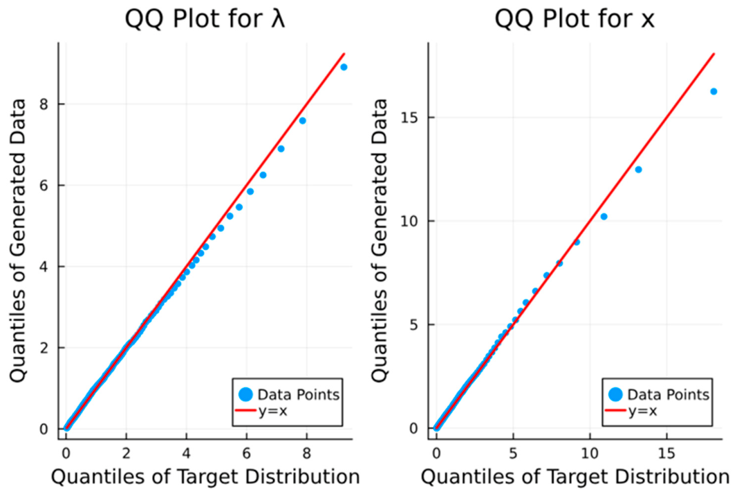
When performing PPM by both perturbing λ and x , we should obtain two exponential distributions, as confirmed in Figure A2.
Figure A2. Samples of the x and λ , generated using PPM in the case of exponential priors for both.
Minerals 16 00736 g0a2

Appendix A.3. Geophysical Inversion with a Gaussian Prior Using GDM or PPM

The above method provides correlated draws from any univariate distribution, continuous or discrete. This idea can be extended to correlated draws from any high-dimensional distribution, if an algorithm to sample from such high-dimensional distribution is available. Consider, for example, the implementation of sampling a Gaussian process on a 2D grid, with given mean and covariance function, using the Cholesky decomposition:
Algorithm A3. Sampling a Gaussian Process using Cholesky decomposition
Input: M e a n   μ ,   c o v a r i a n c e   f u n c t i o n / k e r n e l   C h ;
Output: A single sample x of the G P μ , C h on a N × N grid.
C C h Use covariance function to generate a covariance matrix of size, N 2 × N 2
C = L L T Cholesky decomposition
u   ~   U n i f o r m 0 , 1 Generate N 2 uniform random values
y = F 1 u Calculate N 2   standard Gaussian random values
x = μ + L y Convert independent y into dependent x
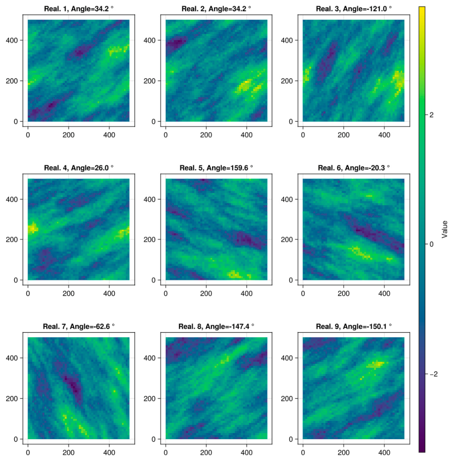
This algorithm generates a vector of independent Gaussian deviates, y . To perturb x , we therefore create perturbations of y . An example is shown in Figure A3. Like in the previous section, we can also perturb parameters of the covariance function. In Figure A4, we show such a case where the azimuth angle is uncertain with a uniform distribution between 1 and 180 degrees.
The perturbations can be used in geophysical inversion. For example, in a Bayesian inversion, the PPM can generate new proposal models in a McMC algorithm. The proposal models are always samples from the prior distribution, if the algorithm to sample from the prior is provided (e.g., a Gaussian prior in Figure A3).
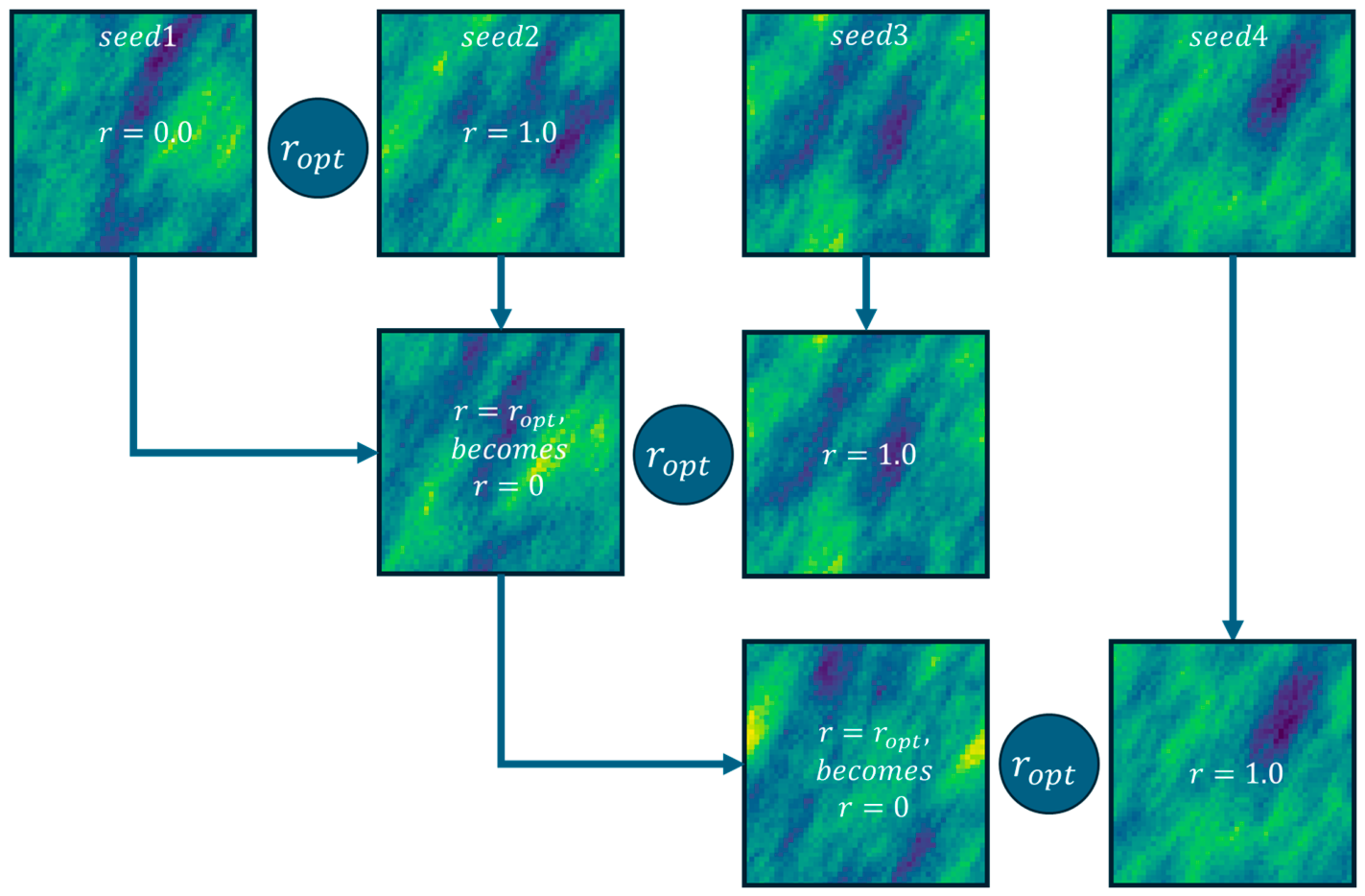
The method can also be used in non-Bayesian stochastic inversion by using PPM as an optimizer, which is the application in this paper. The optimization consists of an outer loop and an inner loop, as visualized in Figure A5. In the outer loop, new realizations of the prior are generated by generating new realizations of a uniform random vector. In the inner loop, the value of r is optimized using a 1D optimization method (such as Dekker–Brent).
Algorithm A4. Stochastic Inversion using PPM with Gaussian prior
Input: d o b s , m i s m a t c h d o b s , m ; m e a n   μ ; c o v a r i a n c e   C
Output: inverted model m ^
u o   ~   U n i f o r m 0 , 1
m o = G a u s s i a n P r i o r A l g o μ ,   C , u o
f o r   i = 1 , , N m a x
u i   ~   U n i f o r m 0 , 1
u o p t 1 D _ o p t i m i z a t i o n m i s m a t c h , d o b s , u i , u i 1
m i = G a u s s i a n P r i o r A l g o μ ,   C , u o p t
end
Return m ^ = m N m a x
Figure A3. Perturbations of Gaussian realizations using PPM, with fixed covariance model.
Minerals 16 00736 g0a3
Figure A4. Joint perturbation of a Gaussian realization and the azimuth angle of the covariance model.
Minerals 16 00736 g0a4
Figure A5. Optimization/inversion with the PPM/GDM consists of an inner and outer loop.
Minerals 16 00736 g0a5
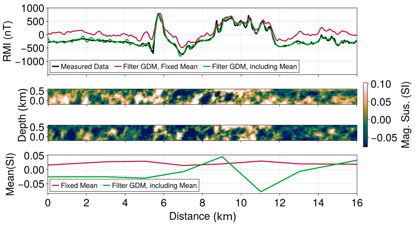
In Figure A6, we see the utility of jointly perturbing the mean of each panel as opposed to fixing the mean. When fixing the mean, the PPM algorithm does not converge to a matching solution. When perturbing the mean from p ( θ | d ) of Equation (22), with θ as the mean, we converge to a solution.
Figure A6. Example of perturbing the mean during gradual deformation (left column, “includes mean”) versus fixing the mean (right column, “fixed mean”). The observed data correspond to one profile of Figure 1. The mean shown in the lower panel is computed as the lateral average of magnetic susceptibility at each depth.
Minerals 16 00736 g0a6

References

  1. Shamsipour, P.; Marcotte, D.; Chouteau, M.; Keating, P. 3D Stochastic Inversion of Gravity Data Using Cokriging and Cosimulation. Geophysics 2010, 75, I1–I10. [Google Scholar] [CrossRef]
  2. Srivastava, R.P.; Sen, M.K. Stochastic Inversion of Prestack Seismic Data Using Fractal-Based Initial Models. Geophysics 2010, 75, R47–R59. [Google Scholar] [CrossRef]
  3. Shamsipour, P.; Marcotte, D.; Chouteau, M. 3D Stochastic Joint Inversion of Gravity and Magnetic Data. J. Appl. Geophys. 2012, 79, 27–37. [Google Scholar] [CrossRef]
  4. Grana, D.; Mukerji, T.; Dvorkin, J.; Mavko, G. Stochastic Inversion of Facies from Seismic Data Based on Sequential Simulations and Probability Perturbation Method. Geophysics 2012, 77, M53–M72. [Google Scholar] [CrossRef]
  5. Pollack, A.; Cladouhos, T.T.; Swyer, M.W.; Siler, D.; Mukerji, T.; Horne, R.N. Stochastic Inversion of Gravity, Magnetic, Tracer, Lithology, and Fault Data for Geologically Realistic Structural Models: Patua Geothermal Field Case Study. Geothermics 2021, 95, 102129. [Google Scholar] [CrossRef]
  6. Grana, D.; Azevedo, L.; De Figueiredo, L.; Connolly, P.; Mukerji, T. Probabilistic Inversion of Seismic Data for Reservoir Petrophysical Characterization: Review and Examples. Geophysics 2022, 87, M199–M216. [Google Scholar] [CrossRef]
  7. Mulè, S.; Soerensen, C.; Munday, T. Handling Noise in AEM Inversion—Implications for Subsurface Characterisation. ASEG Ext. Abstr. 2019, 2019, 1–4. [Google Scholar] [CrossRef]
  8. Vallée, M.A.; Smith, R.S. Inversion of Airborne Time-domain Electromagnetic Data to a 1D Structure Using Lateral Constraints. Near Surf. Geophys. 2008, 7, 63–71. [Google Scholar] [CrossRef]
  9. Oldenburg, D.W.; Haber, E.; Napier, S.; Shekhtman, R. 3D Inversion of Time Domain Data with Integrated Application to Mineral Exploration. In Proceedings of the EGM 2007 International Workshop, Capri, Italy, 15–18 April 2007; European Association of Geoscientists & Engineers: Bunnik, The Netherlands, 2007. [Google Scholar] [CrossRef]
  10. Oldenburg, D.W.; Pratt, D.A. Geophysical Inversion for Mineral Exploration: A Decade of Progress in Theory and Practice. In Proceedings of the Exploration, Toronto, ON, Canada, 9–12 September 2007. [Google Scholar]
  11. Engebretsen, K.W.; Zhang, B.; Fiandaca, G.; Madsen, L.M.; Auken, E.; Christiansen, A.V. Accelerated 2.5-D Inversion of Airborne Transient Electromagnetic Data Using Reduced 3-D Meshing. Geophys. J. Int. 2022, 230, 643–653. [Google Scholar] [CrossRef]
  12. Zhdanov, M.S.; Wan, L.; Jorgensen, M. Joint Three-Dimensional Inversion of Gravity and Magnetic Data Collected in the Area of Victoria Mine, Nevada, Using the Gramian Constraints. Minerals 2024, 14, 292. [Google Scholar] [CrossRef]
  13. Munch, F.D.; Grayver, A. Multi-Scale Imaging of 3-D Electrical Conductivity Structure under the Contiguous US Constrains Lateral Variations in the Upper Mantle Water Content. Earth Planet. Sci. Lett. 2023, 602, 117939. [Google Scholar] [CrossRef]
  14. Mancinelli, P.; Pauselli, C.; Fournier, D.; Fedi, M.; Minelli, G.; Barchi, M.R. Three-Dimensional Gravity Local Inversion Across the Area Struck by the 2016–2017 Seismic Events in Central Italy. J. Geophys. Res. Solid Earth 2020, 125, e2019JB018853. [Google Scholar] [CrossRef]
  15. Szentesy, Z. Geophysical Survey Report, Airborne Magnetic and Helitem2 Survey, Cape Smith Belt Project 2100109B; Assessment Work Submitted to the Government of Québec; GM 72975; 9414-5349; Quebec Inc.: Québec, Canada, 2022; 70p, Available online: https://gq.mines.gouv.qc.ca/documents/EXAMINE/GM72975/GM72975RAP001.pdf (accessed on 9 July 2026).
  16. Scheidt, C.; Li, L.; Caers, J. Quantifying Uncertainty in Subsurface Systems; Geophysical Monograph Series; John Wiley & Sons: Hoboken, NJ, USA, 2018; ISBN 978-1-119-32587-1. [Google Scholar]
  17. Yin, Z.; Strebelle, S.; Caers, J. Automated Monte Carlo-Based Quantification and Updating of Geological Uncertainty with Borehole Data (AutoBEL v1.0). Geosci. Model Dev. 2020, 13, 651–672. [Google Scholar] [CrossRef]
  18. Djuric, P.M.; Kotecha, J.H.; Zhang, J.; Huang, Y.; Ghirmai, T.; Bugallo, M.F.; Miguez, J. Particle filtering. IEEE Signal Process. Mag. 2003, 20, 19–38. [Google Scholar] [CrossRef]
  19. Oliver, D.S. Moving Averages for Gaussian Simulation in Two and Three Dimensions. Math. Geol. 1995, 27, 939–960. [Google Scholar] [CrossRef]
  20. Ravalec, M.L.; Noetinger, B.; Hu, L.Y. The FFT Moving Average (FFT-MA) Generator: An Efficient Numerical Method for Generating and Conditioning Gaussian Simulations. Math. Geol. 2000, 32, 701–723. [Google Scholar] [CrossRef]
  21. Caers, J.; Hoffman, T. The Probability Perturbation Method: A New Look at Bayesian Inverse Modeling. Math. Geol. 2006, 38, 81–100. [Google Scholar] [CrossRef]
  22. Hu, L.Y. Gradual Deformation and Iterative Calibration of Gaussian-Related Stochastic Models. Math. Geol. 2000, 32, 87–108. [Google Scholar] [CrossRef]
  23. Hu, L.Y.; Blanc, G.; Noetinger, B. Gradual Deformation and Iterative Calibration of Sequential Stochastic Simulations. Math. Geol. 2001, 33, 475–489. [Google Scholar] [CrossRef]
  24. Caers, J. Comparing the Gradual Deformation with the Probability Perturbation Method for Solving Inverse Problems. Math. Geol. 2007, 39, 27–52. [Google Scholar] [CrossRef]
  25. Hoffimann, J. GeoStats.Jl—High-Performance Geostatistics in Julia. J. Open-Source Softw. 2018, 3, 692. [Google Scholar] [CrossRef]
  26. Hubert, M.; Debruyne, M. Minimum Covariance Determinant. WIREs Comput. Stat. 2009, 2, 36–43. [Google Scholar] [CrossRef]
  27. Eckstrand, O.R.; Hulbert, L.J. Magmatic nickel-copper-platinum group element deposits. Miner. Depos. Can. Synth. Major Depos. Types Dist. Metallog. Evol. Geol. Prov. Explor. Methods Geol. Asssoc. Can. Miner. Depos. Div. Spec. Publ. 2007, 5, 205–222. [Google Scholar]
  28. Müller, S.; Schüler, L.; Zech, A.; Heße, F. GSTools v1.3: A toolbox for geostatistical modelling in Python. Geosci. Model Dev. 2022, 15, 3161–3182. [Google Scholar] [CrossRef]
  29. Verly, G.W. Sequential Gaussian cosimulation: A simulation method integrating several types of information. In Geostatistics Tróia’92; Springer: Dordrecht, The Netherlands, 1993; Volume 1, pp. 543–554. [Google Scholar]
  30. Sabeti, H.; Moradzadeh, A.; Ardejani, F.D.; Azevedo, L.; Soares, A.; Pereira, P.; Nunes, R. Geostatistical seismic inversion for non-stationary patterns using direct sequential simulation and co-simulation. Geophys. Prospect. 2017, 65, 25–48. [Google Scholar] [CrossRef]
  31. Erten, O.; Pereira, F.P.; Deutsch, C.V. Projection pursuit multivariate sampling of parameter uncertainty. Appl. Sci. 2022, 12, 9668. [Google Scholar] [CrossRef]
  32. Hu, L.Y. Extended Probability Perturbation Method for Calibrating Stochastic Reservoir Models. Math. Geosci. 2008, 40, 875–885. [Google Scholar] [CrossRef]
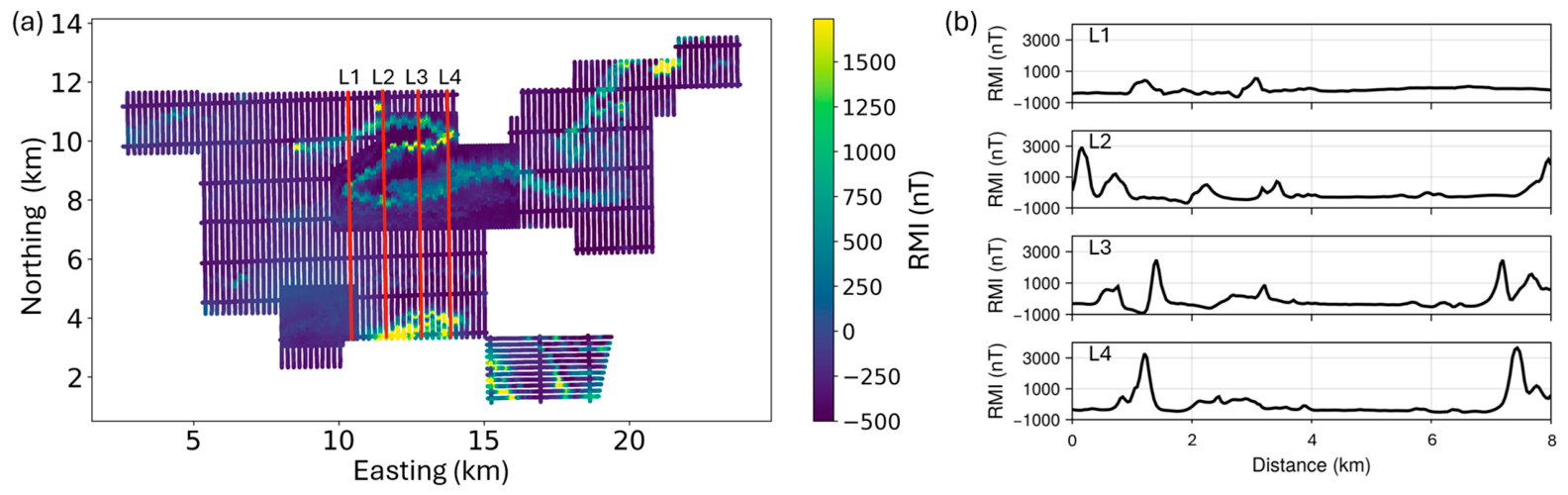
Figure 1. (a) HeliTEM2 total magnetic intensity (in nT) acquired in the Cape Smith belt. (b) The four flightlines analyzed in this study are labelled L1–L4 (red lines); the map axes are given as Easting and Northing in km.
Minerals 16 00736 g001
Figure 2. Sequential Bayesian formulation for a large-scale geophysical inverse problem.
Minerals 16 00736 g002
Figure 3. (ad) Four realizations of magnetic susceptibility. For each panel, the Gaussian-process anisotropy hyperparameters, namely the semi-major axis length, a; the semi-minor/semi-major axis ratio, bf (so the semi-minor axis is b = a × bf); and the ellipse azimuth, γ, together with the petrophysical mean, μ m s , and standard deviation, σ m s , of magnetic susceptibility, were each drawn independently from the uniform priors of Table 1; a single random-field realization was then generated from those sampled values. (1) Bottom (e): The red line is the actual observed magnetic data, and the dark gray lines are the forward-simulated data. On the right (f) is the comparison, in terms of Robust Mahalanobis Distance [17,26], between the observed data and the simulated data. The dashed red line marks the acceptance threshold (95th percentile of the RMD distribution).
Minerals 16 00736 g003
Figure 4. Top (a,b): Geophysical data mapped into a two-dimensional space using multidimensional scaling (MDS); the horizontal and vertical axes, MDS1 and MDS2, denote the first and second multidimensional-scaling coordinates. Shown are the forward-simulated data, as well as the observed data from panels 0 and 1. Bottom (c,d): The relationship between major range and mean of two consecutive panels.
Minerals 16 00736 g004
Figure 5. Procedure for the first panel of L2 flight line (see Figure 1). First row (a), sample hyperparameters from the prior; second row (b), update hyperparameters using the observed magnetic data; third row (c), comparison between observed data, simulated data before GDM, and simulated data after GDM; and fourth row (d), posterior models for the first panel.
Minerals 16 00736 g005
Figure 6. Iteration to the next panel, P1. First row (a), the posterior results of panel P0 (fourth row of Figure 5) carried forward as the starting point for panel P1; second row (b), prediction of the next panel given the previous panel for both hyperparameters and Gaussian model realization; third row (c), comparison between observed data, simulated data before GDM, and simulated data after GDM; and fourth row (d), posterior for the next panel filtered using the gradual deformation method.
Minerals 16 00736 g006
Figure 7. Three inverted magnetic-susceptibility models (ac); shown are the observed data and simulated data after GDM, as well as the variation in the mean and variance of the magnetic susceptibility used in the inversion.
Minerals 16 00736 g007
Figure 8. Top, mean of the ensemble of the inverted models; and bottom, variance of the ensemble.
Minerals 16 00736 g008
Table 1. A broad prior distribution on model variables, as an initial statement of uncertainty. This prior needs to be tested, in a falsification test, with actual observed data.
Prior VariablesDefinitionDistributions
Gaussian process hyper-parameters
2D anisotropy
aLength of the semi-major axis of ellipse, in metersU [200, 700]
bfLength ratio of the semi-minor axis to the semi-major axis in an ellipse, the length of semi-minor axis b = abfU [0.01, 1]
γAzimuth angle of ellipseU [1, 180]
PetrophysicsμmsMean value magnetic susceptibilityU [0, 0.3]
σmsStandard deviation magnetic susceptibilityU [0.05, 0.5]
Disclaimer/Publisher’s Note: The statements, opinions and data contained in all publications are solely those of the individual author(s) and contributor(s) and not of MDPI and/or the editor(s). MDPI and/or the editor(s) disclaim responsibility for any injury to people or property resulting from any ideas, methods, instructions or products referred to in the content.