


Abstract
Accurate quantification of mineralogical composition in carbonate rocks is essential for reservoir characterization in the oil industry, directly influencing petrophysical properties such as porosity and permeability. However, traditional methods such as X-ray diffraction (XRD) are destructive and provide limited spatial sampling. The aim of this study was to develop and validate a workflow for the continuous quantification of calcite and dolomite in drill cores from the Brazilian pre-salt oil province by integrating short-wave infrared (SWIR) hyperspectral imaging (HSI) and Machine-Learning algorithms. A total of 80 m of cores were evaluated using 170 XRD-validated samples to calibrate linear, nonlinear, and ensemble models. The results showed that the combination of Multiplicative Scatter Correction (MSC) preprocessing with Multilayer Perceptron (MLP) and Support Vector Regression (SVR) achieved the best performance, reaching an of 0.84. Explainable Artificial Intelligence (SHAP) confirmed the relevance of diagnostic bands between 2330 and 2360 nm, improving geological interpretability of the predictions. The proposed methodology provides a non-destructive and high-resolution alternative for mineralogical profiling, supporting the evaluation of complex reservoirs and decision-making in the oil and gas industry. Although the workflow was validated using a specific pre-salt dataset, future studies should assess its transferability to other carbonate reservoirs and broader geological settings.
1. Introduction
Carbonate reservoirs host a substantial proportion of the world’s hydrocarbon reserves and are of major strategic importance for global energy supply. Representative examples include giant petroleum systems in the Middle East, North America, Asia, and the Brazilian pre-salt province. Despite their economic relevance, carbonate reservoirs commonly exhibit strong heterogeneity related to depositional facies, diagenetic processes, pore systems, and mineralogical variability, which makes their characterization particularly challenging. The mineralogical composition of carbonate rocks, particularly the proportion of calcite () and dolomite (), plays a strong role in determining the petrophysical and mechanical properties of these materials. In petroleum geology, for example, the presence and distribution of these minerals can directly influence porosity and permeability and thus the storage and flow capacity of hydrocarbons in reservoirs [1]. Dolomitization, a diagenetic process involving the replacement of calcium ions by magnesium in the calcite crystalline structure, is frequently associated with improved reservoir quality due to the creation of secondary porosity [2]. Understanding and accurately quantifying the abundance of these minerals is therefore essential for the exploration, evaluation, and management of natural resources.
Traditionally, mineralogical quantification has been performed using laboratory techniques such as X-ray diffraction (XRD) [3]. XRD is a powerful tool that provides detailed crystallographic information and allows for the quantitative determination of mineral phases with high accuracy [4]. However, XRD is a technique that requires careful sample preparation, is time-consuming, and is not suitable for field or large-scale analyses [3]. Furthermore, the destructive nature of XRD sampling can be a limitation in scenarios where sample integrity is critical.
Given the inherent limitations of traditional methods, the advancement of Remote-Sensing technologies, notably hyperspectral imaging (HSI), has established itself as a promising alternative for mineralogical characterization. Hyperspectral sensors record reflectance in hundreds of narrow, contiguous spectral bands, covering a large portion of the electromagnetic spectrum, especially in the visible to short-wave infrared region (400–2500 nm), enabling the identification and detailed mapping of minerals on the Earth’s surface [5,6]. This capability stems from the fact that each mineral has a characteristic spectral signature that allows its identification and, in some cases, its quantification [7].
In the specific case of carbonates, the Shortwave Infrared (SWIR) region is particularly relevant, as the vibrational transitions of the anion generate diagnostic absorption features around 2300 nm [5,6,8]. Calcite typically exhibits an absorption band centered approximately between 2330 and 2340 nm, while dolomite displays a slightly shifted feature at shorter wavelengths, around 2310–2320 nm [5,6]. This difference in the absorption bands’ position is the key to spectral discrimination between the two minerals. However, in mixed mineral systems, these absorption features may be affected or partially obscured by the presence of phyllosilicates, which can modify the SWIR spectral response. In such cases, complementary absorptions near 2500 nm may provide additional robustness for carbonate identification.
The relevance of HSI can be even more evident in complex environments, such as carbonate reservoirs of the pre-salt layer, where mineralogical and textural heterogeneity is present [9]. In this context, the transition from laboratory analyses of discrete samples to continuous core imaging represents an advantage that makes HSI a promising technology in mineral exploration. The ability of HSI to discriminate carbonate minerals based on their spectral signatures, combined with the imaging nature of the technique, allows for a non-destructive and continuous analysis of mineralogical composition throughout an entire core [10,11]. This approach generates a continuous mineralogical record, allowing the identification of compositional variations and the direct correlation with geological features observed in the core [12].
The literature has explored this connection between hyperspectral data and carbonate rocks, with a growing focus on the application of quantitative and automated methods. Initially, studies concentrated on the fundamental spectral characterization of carbonates. Works such as those carried out by Zaini et al. (2012) [13] were crucial in establishing the basis of spectral knowledge for the study of these minerals, investigating how physical factors, such as grain size and mineral admixture, influence the absorption features of calcite and dolomite in the SWIR and Thermal Infrared (TIR) regions. The authors demonstrated that the position of absorption bands in the SWIR is relatively invariant to grain size but sensitive to the proportion of calcite and dolomite, providing a proxy for the evaluation of dolomitization patterns.
Moving towards practical application, laboratory-based hyperspectral imaging was first explored for the determination of carbonate rocks’ chemistry. Zaini et al. (2014) [14] used the SisuCHEMA scanner to estimate the chemical composition between calcium and magnesium and the relative abundance of carbonate minerals in hand samples. This study compared wavelength-position-based approaches, Spectral Angle Mapper—SAM—and Linear Spectral Unmixing—LSU—concluding that the wavelength-position approach was more stable and reproducible for estimating mineral chemistry. Such studies validated HSI as a high-resolution tool for mineralogical characterization on a laboratory scale, paving the way for its application in borehole cores.
From the mid-2010s onwards, the integration of HSI with Machine Learning (ML) emerged as a paradigm to overcome the limitations of purely spectral methods, especially in complex and heterogeneous samples. The high dimensionality of hyperspectral data, while rich in information, demands robust methods for feature extraction and predictive modeling. Tuşa et al. (2020) [15] proposed an ML framework to estimate mineral abundance in borehole cores, combining hyperspectral data with high-resolution mineralogical data obtained by scanning electron microscopy—mineral liberation analysis. The work demonstrated the ability of ML algorithms, such as Random Forest and Support Vector Machine, to extrapolate point data to the continuous scale of the core. In 2021, De La Rosa et al. [16] reinforced this trend by applying an ML-based approach to map mineral abundance in deposit-scale borehole cores using hyperspectral data. The study highlighted the ease of transposing this approach to different deposits, underlining the scalability and robustness of ML models in interpreting large volumes of core logging data. More recently, research has focused on the optimization and interpretability of these models. Wei et al. (2024) [17] proposed a hybrid method that integrates spectral knowledge with ML for estimating dolomite content in outcrops. The use of a feature selection based on spectral knowledge, followed by ML algorithms, resulted in high accuracy and, crucially, greater model interpretability, an aspect that is becoming increasingly important in the application of ML techniques in geosciences. Consequently, current research seeks models that not only accurately predict mineral content but also provide geological insights into the relationship between spectral response and mineral composition.
Despite advancements, the application of HSI and ML in quantifying carbonates in borehole cores still faces significant challenges. Most studies focus on black-box models, where many ML models, especially more complex ones like Deep Neural Networks, offer high accuracy but lack interpretability. In geosciences, the ability to trace predictions back to diagnostic spectral features is fundamental for geological validation and user confidence. Furthermore, the robustness and generalization of carbonate quantification models in the face of variations in spectral preprocessing, mineralogical heterogeneity, and different data acquisition conditions remain an open question. Preprocessing optimization is also a critical point, as the choice of spectral technique (e.g., Continuum Removal, Derivatives, MSC) has a significant impact on model performance, but the literature lacks a systematic and comparative evaluation of how different preprocessing methods can affect the accuracy and stability of multiple ML algorithms for the quantification of calcite and dolomite.
In summary, although hyperspectral imaging in drill cores combined with ML has been established as a powerful tool for non-destructive mineralogical characterization, there is a gap in the literature regarding the systematic evaluation of the robustness and interpretability of predictive models for carbonate quantification. The need for models that are not only accurate but also geologically transparent and stable across different preprocessing strategies represents a research challenge.
The present work aims to fill this gap by proposing a robust and systematic evaluation of multiple ML algorithms, ranging from linear models (such as Partial Least Squares Regression—PLSR and Ridge Regression) to nonlinear and ensemble models (such as Support Vector Regression—SVR, Random Forest, and Multilayer Perceptron—MLP), combined with different spectral preprocessing techniques. The central goal is to identify the preprocessing and algorithm combination that offers the best balance between predictive accuracy and robustness for calcite and dolomite quantification in drill cores from carbonate reservoirs of the Brazilian pre-salt interval.
Additionally, the study addresses the issue of interpretability by employing eXplainable Artificial Intelligence (XAI) techniques, such as variable importance analysis, to ensure that the model’s predictions are traceable to the diagnostic spectral features of carbonates. By providing a comparative analysis and incorporating interpretability, this work stands as an advance in the literature, offering an optimized and transparent workflow for the quantification of carbonates in mineral exploration. The results of this research provide guidelines for the implementation of hyperspectral core logging routines that provide improvements to borehole data quality and significance for the characterization of complex reservoirs.
2. Materials and Methods
2.1. Data Acquisition
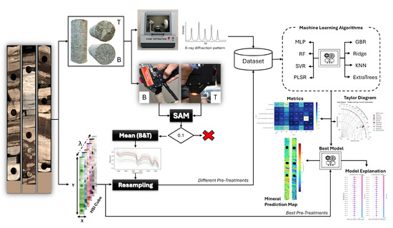
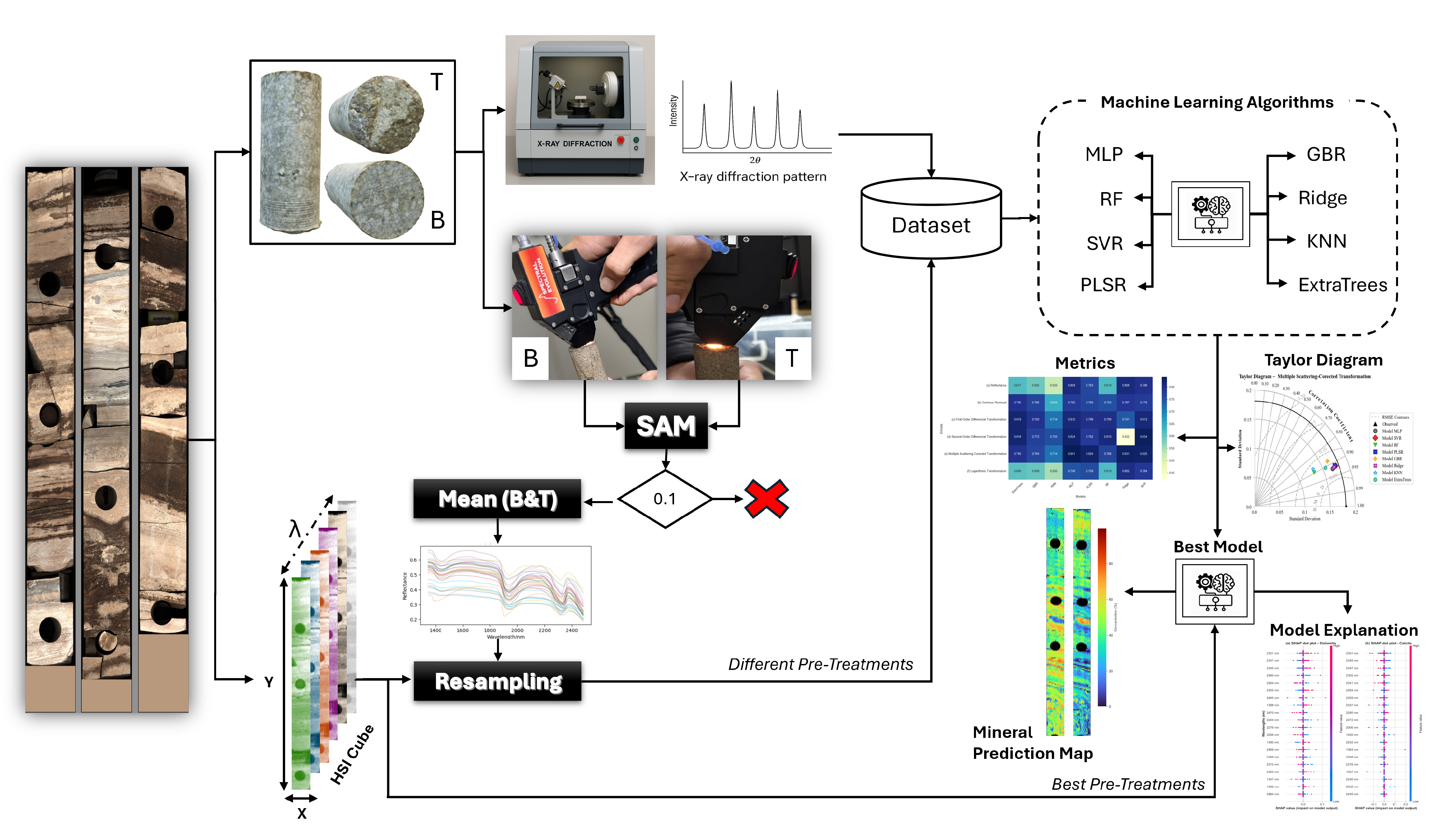
The methodology of this study, illustrated in Figure 1, is based on a dataset of drill cores from a pre-salt carbonate field provided by Petróleo Brasileiro S.A. (Petrobras, Rio de Janeiro, Brazil). These pre-salt reservoirs are mainly composed of carbonate rocks, with high concentrations of calcite and dolomite, typical of microbialite formations [9]. A total of 80 m of core samples were analyzed. These had been previously digitized using an automated workflow with a Multi-Sensor Core Logger (MSCL), which enables the simultaneous acquisition of different measurements along the cores. During this process, the cores are placed on a motorized conveyor belt, and various sensors collect data at discrete, depth-registered intervals. This setup ensures spatial alignment across datasets, supporting their standardization and integration within a unified reference system. For further information on the digitization workflow, see [18].
Figure 1.
Methodological flowchart for carbonate quantification in drill cores. The diagram illustrates the complete modeling process, beginning with data acquisition (drill cores and T/B plugs) and X-ray diffraction (XRD) analysis. The workflow proceeds with hyperspectral reflectance measurement, homogeneity validation using Spectral Angle Mapper (SAM), and spectral resampling. The core stage involves the application of multiple Machine-Learning algorithms and performance evaluation, culminating in the selection of the best model, generation of the mineral prediction map, and model explainability analysis.
From the digital archive available dataset, hyperspectral reflectance images acquired by the SPECCAM 4 sensor (Geotek, Daventry, UK) were used. This sensor operates in the SWIR range, from 1300 nm to 2500 nm, with 301 spectral bands corresponding to an average spectral sampling interval of approximately 4 nm and a pixel size of 0.5 mm × 3 mm. The non-square pixel geometry is associated with the original line-scanning acquisition configuration adopted during core digitization, in which spatial sampling differs between the scan axis and the conveyor–motion axis. Detailed operational parameters such as scan speed and hardware settings were not available to the authors, since the dataset was previously acquired and provided as part of an institutional digital archive. Additionally, for the purpose of validating the results, measurements obtained with the Vanta Max X-ray fluorescence (XRF) sensor (Evident, Waltham, MA, USA) were used. This sensor is configured with a 4 W X-ray tube and a rhodium anode operating between 8 and 50 kV, with all measurements properly co-registered by depth.
In addition to the provided datasets, the study incorporated high-resolution mineralogical and spectral analyses based on discrete samples. Prior to the digitization of the cores, a total of 214 plugs were collected, selected from regions of interest along the core. From these plugs, subsamples were extracted for X-ray diffraction (XRD) analysis to serve as a mineralogical composition reference. It is important to note that although calcite, dolomite, and quartz have been identified during the XRD analyses, quartz concentration in the cores was consistently very low compared to the carbonate mineral content. For this reason, the present study focused exclusively on the quantification and assessment of carbonate minerals.
Subsequently, the same 214 plugs have been subjected to point-based spectral measurements on their top and bottom surfaces using a portable spectroradiometer with high spectral resolution. The spectroradiometer employed was the Spectral Evolution RS-3500 sensor (Spectral Evolution Inc., Haverhill, MA, USA), which operates over the spectral range from 350 to 2500 nm, covering a total of 2151 spectral bands.
A summary of the main dataset characteristics and analytical data used in this study is presented in Table 1.
Table 1.
Summary of the core dataset and analytical data used in this study.
To ensure consistency and reliability of the data used for modeling, particularly considering the possibility of heterogeneous plugs, a sample homogeneity validation workflow was implemented. This assessment was based on the comparison of the spectral signatures obtained from the top and bottom surfaces of each plug using the SAM algorithm.
SAM is a mathematical method used to quantify the spectral similarity between two spectra by calculating the angle between them. This method was chosen considering SAM’s ability to remain unaffected by spectral intensity, focusing primarily on the shape of the spectral signature. This makes it particularly effective for identifying materials under varying illumination conditions [19]. Equation (1) details the mathematical process of the method:
where represents the number of spectral bands, r is the reference spectrum, and t is the spectrum to be evaluated.
For the sample homogeneity validation step, after applying the SAM algorithm, the level of similarity between the top and bottom spectral signatures of each plug was assessed. Plugs in which the spectral angle between the top and bottom was below a predefined threshold were considered homogeneous and, therefore, suitable for inclusion in the modeling process. In contrast, plugs that showed SAM values above this threshold were systematically excluded from the dataset. This approach was implemented to minimize the influence of heterogeneous samples, which could introduce false negatives or significantly compromise the accuracy and robustness of the modeling results, especially given the lack of precise information regarding the exact location from which the XDR analysis samples were extracted within each plug.
A threshold of 0.10 radians was defined as the decision criterion. This choice was based on a sensitivity analysis of different threshold values. It was observed that lower thresholds, such as 0.05 radians, led to the undue exclusion of samples affected by minor variations at the beginning and end of the spectral signatures, which may result from instrumental fluctuations. On the other hand, higher values, such as 0.15 radians, allowed differences that were more indicative of acceptable heterogeneity. The 0.10-radian threshold proved to be the most suitable, as it preserved the similarity between the top and bottom spectral signatures of the plugs while eliminating major discrepancies. After this filtering process, a total of 170 plugs were selected. For these plugs, the average of the top and bottom spectral signatures was computed and used in the subsequent preprocessing step.
2.2. Spectroscopy Pre-Treatments and Dataset Creation
After selecting the 170 plugs and computing their spectral averages, the preprocessing step was carried out. The first phase of this process consisted of resampling the spectral signatures. Since the prediction models generated by the end of the experiment would be applied to the hyperspectral images of the cores, the 170 spectral signatures obtained with the portable spectroradiometer Spectral Evolution RS-3500 were resampled to match the spectral resolution of the images acquired by the SPECCAM 4 sensor.
The adopted resampling technique is based on modeling the spectral response of the target sensor, in which each band is represented by a Gaussian function centered at the target wavelength and characterized by its full width at half maximum (FWHM) [20,21]. Its mathematical formulation is based on the principle that, given a series of spectral points , where represents the wavelength and the reflectance at that wavelength, and a new set of wavelengths at which the reflectance is to be estimated, the resampling is defined by Equation (2):
The weights reflect the degree of overlap between the Gaussian function of the target band and the original wavelengths, and are given by
with the standard deviation related to the width at half height by
Following the resampling step, different types of preprocessing methods were evaluated, since preprocessing can have a significant impact on the generalization ability of Machine-Learning-based methods [22]. In addition, selecting the appropriate preprocessing technique can improve modeling accuracy, whereas an incorrect choice may lead to unreliable predictions [23]. In this context, four distinct preprocessing methods have been evaluated along with the original spectra (ORI), namely: Continuum Removal (CR) [24], First Derivative Transformation (FDT) [25], Second Derivative Transformation (SDT) [26,27], and MSC [28]. The preprocessing methods are expressed by the following equations:
where is the continuum reflectance at wavelength , and is the reference spectrum, generally taken as the mean spectrum of all samples.
Based on the resampled spectral averages, the final dataset integrated, for each plug, the four preprocessed versions of the signatures along with the original signature (ORI, CR, FDT, SDT, and MSC), as well as the reference responses from XRD (dolomite and calcite). This allowed for the evaluation of the impact of each preprocessing method on predictive performance and the identification of the most suitable configuration for carbonate estimation.
2.3. Spectral Model Development
To quantify dolomite and calcite from hyperspectral signatures, a set of complementary algorithms was adopted, including linear models, non-linear models, tree-based ensemble methods, and an instance-based method.
Among linear methods, the PLSR and Ridge Regression algorithms were evaluated. Applied to chemometric analyses [29], PLSR is a multivariate linear modeling technique that relates predictors to the response and successively extracts orthogonal latent factors selected to maximize the covariance between spectral measurements and the measured chemical property [30]. Given a predictor matrix and a response matrix , PLSR seeks a linear relationship of the form
where is the regression coefficient matrix. PLSR is particularly well-suited for datasets with high dimensionality and multicollinearity [31]. Still within the scope of linear models, Ridge Regression is a linear regression method that incorporates an penalty into the regression cost function [32]. This regularization shrinks the coefficients toward zero, reducing the estimator’s variance and mitigating multicollinearity [33]. The cost function minimized by Ridge Regression is defined as
where is the coefficient vector, is the predictor matrix, is the response vector, and is the regularization parameter that controls the strength of the penalty. The solution for the coefficients is given by
where is the identity matrix.
Regarding non-linear methods, SVR and MLP were evaluated. SVR is considered an extension of Support Vector Machine (SVM), which is commonly used for classification problems. It aims to find a function that fits the regression data while allowing an error margin for the predictions and at the same time seeks the simplest possible function [34]. The SVR optimization problem is formulated as
where is the weight vector, b is the bias, maps the data to a (possibly) high-dimensional feature space, C is the penalty parameter, is the width of the epsilon-insensitive tube, and are the slack variables that quantify violations above and below the tube. The strength of SVR lies in its ability to handle non-linear relationships between input and output variables, using a kernel function to map the data into a high-dimensional feature space where linear regression can be applied [35].
Within the context of Artificial Neural Networks (ANNs), MLP is a feedforward network characterized by the presence of multiple interconnected layers, processing information in a single direction from input to output [36]. Its training is carried out using error backpropagation algorithms with numerical optimization, which iteratively adjust the connection weights to minimize the difference between the predicted outputs and the actual values [37]. The output of a neuron j in layer l is computed as
where g is the activation function (e.g., ReLU, sigmoid), are the weights connecting neuron k in layer to neuron j in layer l, is the output of neuron k in the previous layer, and is the bias of neuron j. MLP training is performed via error backpropagation.
In addition to the different types of regression evaluated, the analysis was expanded to include ensemble algorithms. These methods, which combine the predictions of multiple models, were represented by three Decision Tree-based approaches: Random Forest Regression—RF, Extra Trees, and Gradient Boosting Regressor—GBR.
RF is based on the combination of a set of Decision Tree Regressors. Decision Tree Regression is a supervised model that recursively partitions the data, learning at each node the splitting rules that maximize the gain until stopping criteria are met, assigning a label or prediction value to the leaves [38]. Unlike a single Decision Tree, which can be prone to overfitting due to its recursive data-splitting structure, RF mitigates this risk by constructing a forest of trees [39]. For an input , the RF prediction is the average of the predictions from all K trees in the forest:
where is the prediction of the k-th tree. Extra Trees is similar to RF but introduces greater randomness in the construction of the trees by selecting split points randomly for each feature. This extreme randomness in choosing split points and sampling the data helps reduce the model variance, resulting in a slightly higher bias but significantly lower variance compared to RF [40,41].
Constructed from a set of sequentially arranged Decision Trees, GBR is a regression model in which each new Decision Tree is trained to correct the errors of the previously built trees so that the next tree learns from the errors of the preceding model [42]. The process involves optimizing a loss function using a gradient descent algorithm, adjusting the weights and predictions of each tree to minimize the overall error [42,43]. The final prediction is a weighted sum of the predictions from the trees:
where are the base functions, and are the weights that minimize the loss function at each stage.
Finally, as an instance-based method, the K-Nearest Neighbors (KNN) algorithm was evaluated. KNN is a non-parametric algorithm that can be used for both classification and regression, basing its predictions on the proximity of points in the feature space [44]. For regression, the prediction for a new instance is given by the average of the target values of the k nearest instances in the training set:
where denotes the set of the k nearest neighbors of . The choice of k is crucial and directly affects the bias, variance, and sensitivity to noise [44]. One of the main advantages of KNN is its simplicity and adaptability to complex distributions; however, its performance may degrade in high-dimensional spaces [45].
2.4. Model Evaluation
To evaluate the consistency and performance of the prediction models, an approach combining quantitative evaluation metrics with statistical tests was adopted.
The first evaluation step focused on the purely mathematical analysis of the results, using widely recognized metrics in the context of data prediction, such as the score and the Root Mean Square Error (RMSE). The score is a statistical measure that represents the proportion of variance in the dependent variable that is predictable from the independent variable [46]. Values closer to 1 indicate that the model explains a greater proportion of the data variability, suggesting a good fit. Its formulation is given by
where represents the actual value, the predicted value, and the mean of the actual values.
RMSE is a metric that allows measuring the magnitude of errors produced by a prediction model. It represents the square root of the mean of squared errors and is particularly useful because it penalizes larger errors more significantly, being expressed in the same unit as the predicted variable, which facilitates interpretation [47]. Lower RMSE values indicate higher model accuracy. Its equation is given by
In addition to the metrics presented above, the Taylor Diagram was also employed to complement the evaluation of the results. The Taylor Diagram is a graphical tool that enables quality visual comparison of different models against a reference dataset [48]. It allows for the simultaneous comparison of three statistical metrics: the Pearson correlation coefficient, which indicates the degree of alignment between predicted and observed values; the standard deviation—SD—which shows the preservation of data variability; and the Root Mean Square Difference (RMSD), which represents the average deviation after bias removal. The equations for calculating Pearson and RMSD are presented below.
where and represent the standard deviation of the predicted value and the actual value, respectively.
Although descriptive statistical analysis provides insights into the models’ relative performance, only inferential statistical analysis allows us to infer which models stand out under a defined significance level. Thus, as a second step, non-parametric tests were employed, such as (1) the Friedman test, to assess overall differences among average ranks; and (2) the Nemenyi post hoc test to identify which pairs of models differ significantly.
The Friedman test is a non-parametric statistical method used to compare the performance of three or more algorithms across multiple datasets. It operates by ranking the algorithms for each dataset and calculating their average ranks. The goal is to determine whether the observed differences in these average ranks are statistically significant [49]. The Friedman test statistic, , is calculated using the following formula:
where N is the number of datasets, k is the number of algorithms, and is the average rank of the j-th algorithm. A significant Friedman result indicates performance differences, but it does not specify which algorithms differ.
To identify which algorithms are significantly different following a significant Friedman test result, the Nemenyi post hoc test is used. This test calculates a critical difference (CD), which serves as a threshold for pairwise comparisons [50]. If the absolute difference between the average ranks of two algorithms exceeds the CD, the difference is considered statistically significant. The formula for CD is
In this equation, are values based on the Studentized range distribution [51]. If , algorithms i and j are considered significantly different.
2.5. Model Explanation
In order to provide greater explainability of the best combinations of preprocessing techniques and prediction models adopted, XAI techniques were employed. As an XAI technique, SHapley Additive exPlanations (SHAP) was used. Based on game theory, SHAP measures the impact of each feature on the predictions by considering all possible combinations of features and their respective contributions [52]. Features with greater effect on the model receive higher importance rankings, while those with less influence are ranked lower [23,52].
SHAP values measure the marginal contribution of each feature to the prediction, considering all possible combinations of features [53]. The equation for the SHAP value of each feature i is given by
where F is the set of all features; S is a subset of F that does not contain feature i; is the number of features in S; is the total number of features; is the model prediction when the feature set S and feature i are present; and is the model prediction when only the set S is present (i.e., with feature i absent).
It is worth noting that SHAP values provide a more comprehensive and interpretable measure of feature importance than conventional metrics, as they simultaneously account for the direction, magnitude, and interactions among features [23,52].
2.6. Visualization of the Distribution of Response Attributes
To apply and validate the models developed for the quantification of dolomite and calcite, it is possible to predict the concentrations of these minerals in the hyperspectral images of the cores. The workflow consists of extracting the spectral signature of each pixel and applying the best combinations of preprocessing and models selected in the previous step. The resulting predictions are then mapped back to their original spatial positions, resulting in two-dimensional maps of dolomite and calcite.
The maps allow visualization of spatial distribution along the core and enable the evaluation of model performance in a practical scenario. Since the hyperspectral images and the XRF data are properly co-registered to depth (Section 2.1), cross-validation between the results is possible. The chemical composition of calcite () is predominantly calcium (Ca), while dolomite () is rich in both calcium and magnesium (Mg). Therefore, the presence of magnesium serves as a chemical indicator (proxy) for dolomite abundance. Based on this, the Ca and Mg measurements from the XRF sensor were used as a reference for external validation of the predictions.
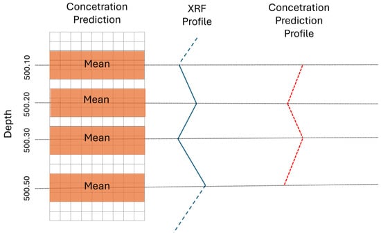
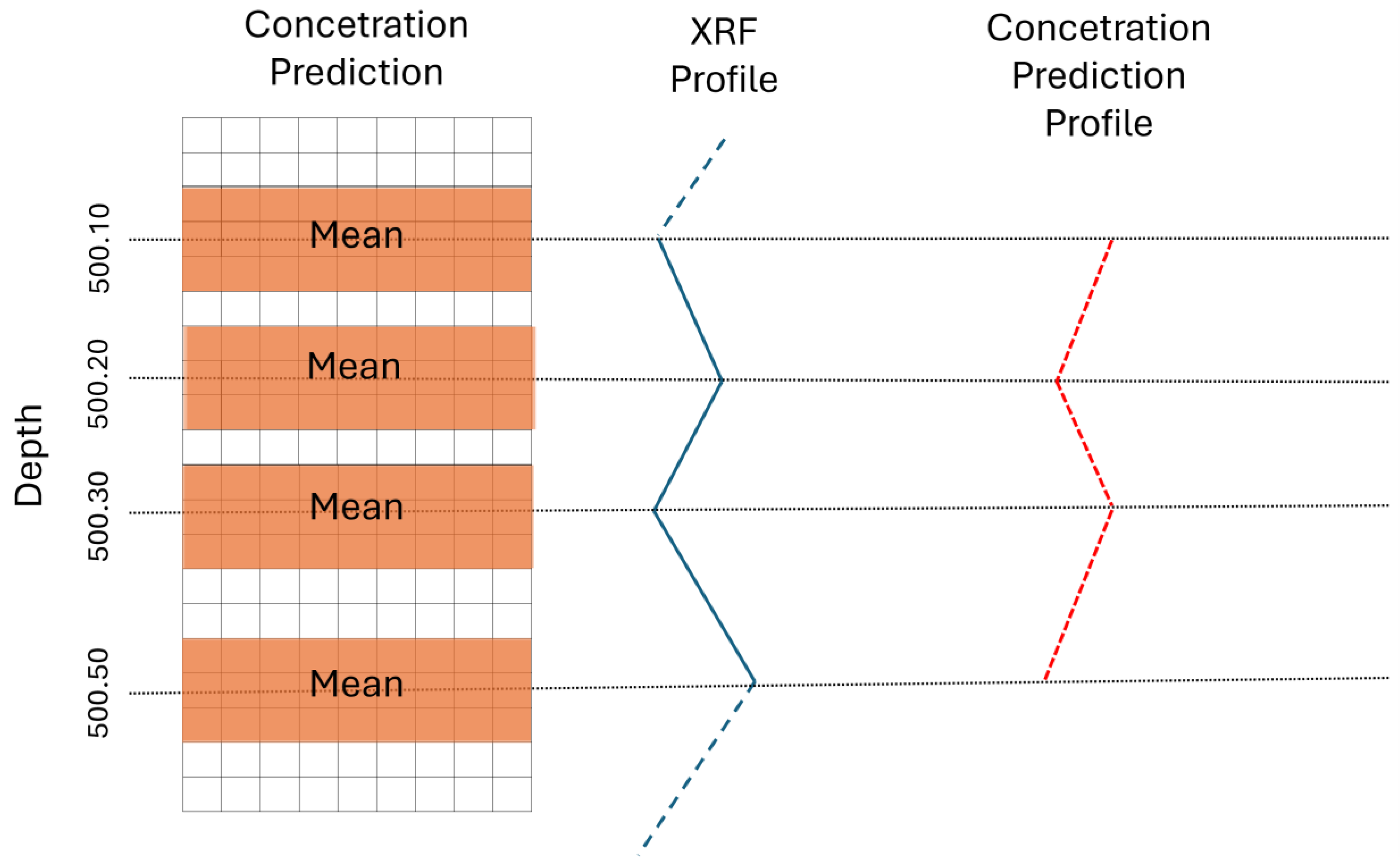
To ensure a fair comparison, an average concentration profile of the predicted minerals with respect to depth was generated and aligned with XRF measurements. This profile was constructed by estimating the average concentration within a pixel window surrounding each XRF measurement point. Specifically, for each depth with an XRF measurement, three pixel rows above and three below the corresponding row were selected, and the average of the predicted mineral concentrations within this window was calculated. The result is a continuous concentration profile along depth, analogous to the geochemical profile from XRF. Figure 2 illustrates the procedure performed.
Figure 2.
Data alignment scheme for statistical comparison. The diagram illustrates the procedure for aligning the concentration profile predicted by the Machine-Learning model (prediction profile) with the X-ray fluorescence measurements (XRF profile). The alignment is performed by comparing the predicted mean concentration profile (mean) within a pixel window around the XRF measurement point, ensuring a fair and statistically valid basis for comparison between the methods.
With the XRF and predicted concentration profiles, comparisons can be made using correlation metrics, such as Pearson correlation (Equation (17)), in order to assess the relationship between chemical concentration and the predicted mineral concentration.
2.7. Computational Environment
All scripts developed for this study were implemented in Jupyter Notebook using the Python 3.9 programming language. The libraries used included pandas for data manipulation and analysis, NumPy for vector and matrix operations, scikit-learn for Machine-Learning algorithms, Matplotlib for data visualization, Spectral Python for hyperspectral image processing and analysis, and the SHAP library for computing SHAP explanations. Hypothesis testing was performed in R software with the support of the tsutils package. The computational setup consisted of an Alienware notebook equipped with an 11th-generation Intel® Core™ i7-11800H processor (2.30 GHz), 32 GB of RAM, and a dedicated 8 GB graphics processing unit (GPU), running on a 64-bit Microsoft Windows system.
3. Results
3.1. Spectral Characteristics and Preprocessing
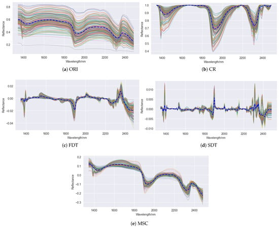
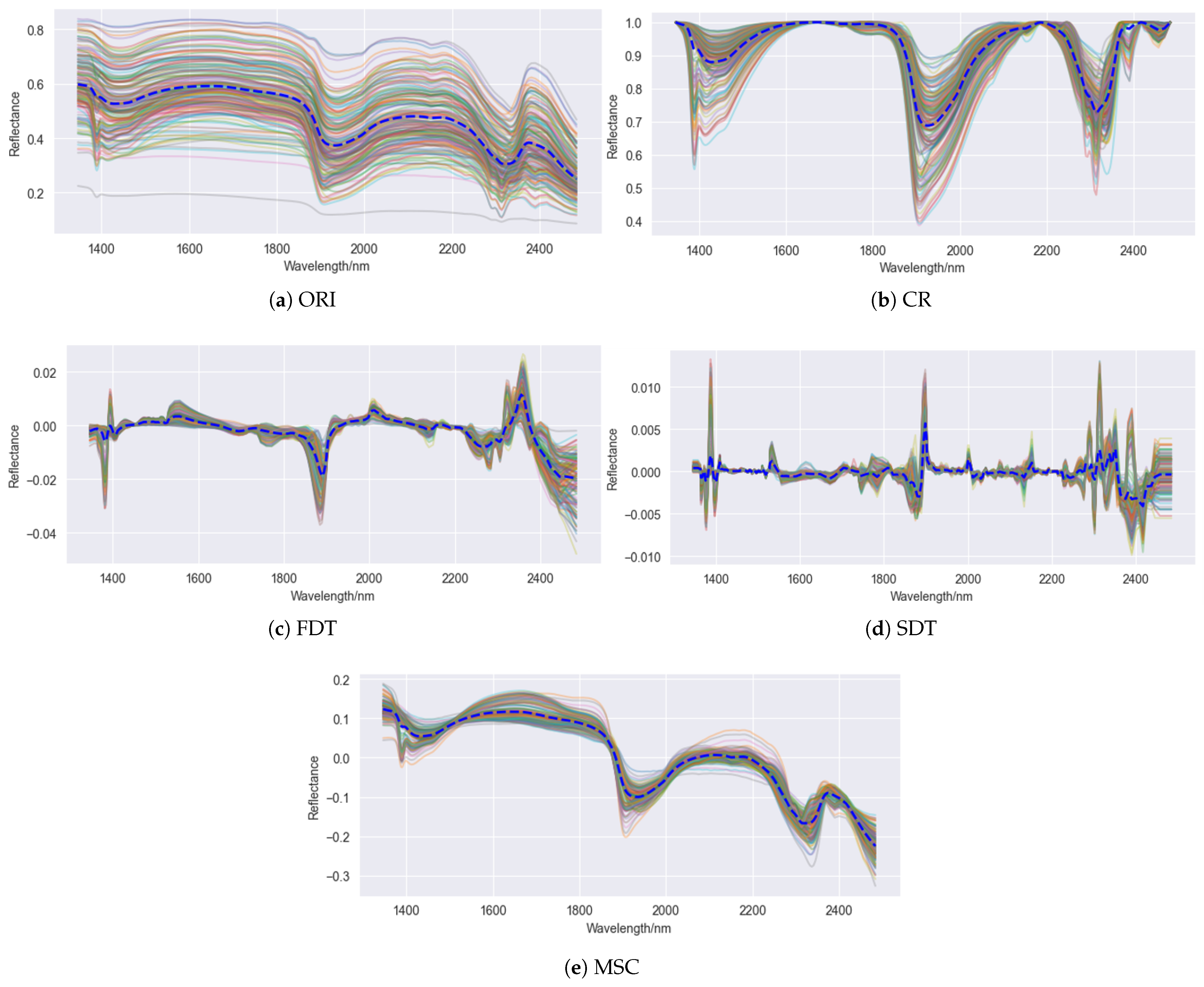
Figure 3 presents the results of the spectral transformations applied to the hyperspectral dataset used in this study. As observed in Figure 3a, the ORI exhibits a continuous variation pattern ranging approximately from 0.25 to 0.80, with few spectra exceeding these limits. Most spectra are in concise agreement, highlighting common features, such as absorption valleys around 1400 and 1900 nm, which are typical of () molecules absorption in mineral structures [7,31]. Additionally, features between 2300 and 2350 nm stand out, associated with internal molecular vibrations of carbonate ions () [6,7,54].
Figure 3.
Visualization of the hyperspectral signatures collected for all samples. The blue dashed line represents the mean of all signatures. (a) Original signature; (b) signature with continuum removed; (c) signature transformed by the first derivative; (d) signature transformed by the second derivative; and (e) signature after applying Multiplicative Scatter Correction.
The spectral transformations CR, FDT, SDT, and MSC reveal different aspects of the spectral signatures. CR emphasized diagnostic bands by removing the global trend of the spectra, enhancing the differences between absorption features at 1410, 1920, and 2335 nm. The derivative transformations increased the resolution of peaks and valleys, especially in central regions, although the second derivative introduces greater noise at the edges. The MSC reduced variations caused by scattering effects, thereby minimizing influences not related to the samples’ chemical composition.
These preprocessing techniques highlighted spectral regions of interest, particularly the range between 2300 and 2350 nm, which is consistent with the presence of carbonate minerals such as calcite and dolomite. These regions are already widely recognized in the literature as diagnostic bands for these minerals, reinforcing both the relevance of the dataset used and the effectiveness of the applied transformations for spectral modeling purposes.
3.2. Analysis of the Geochemical Data
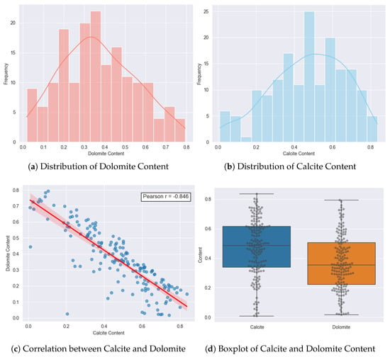
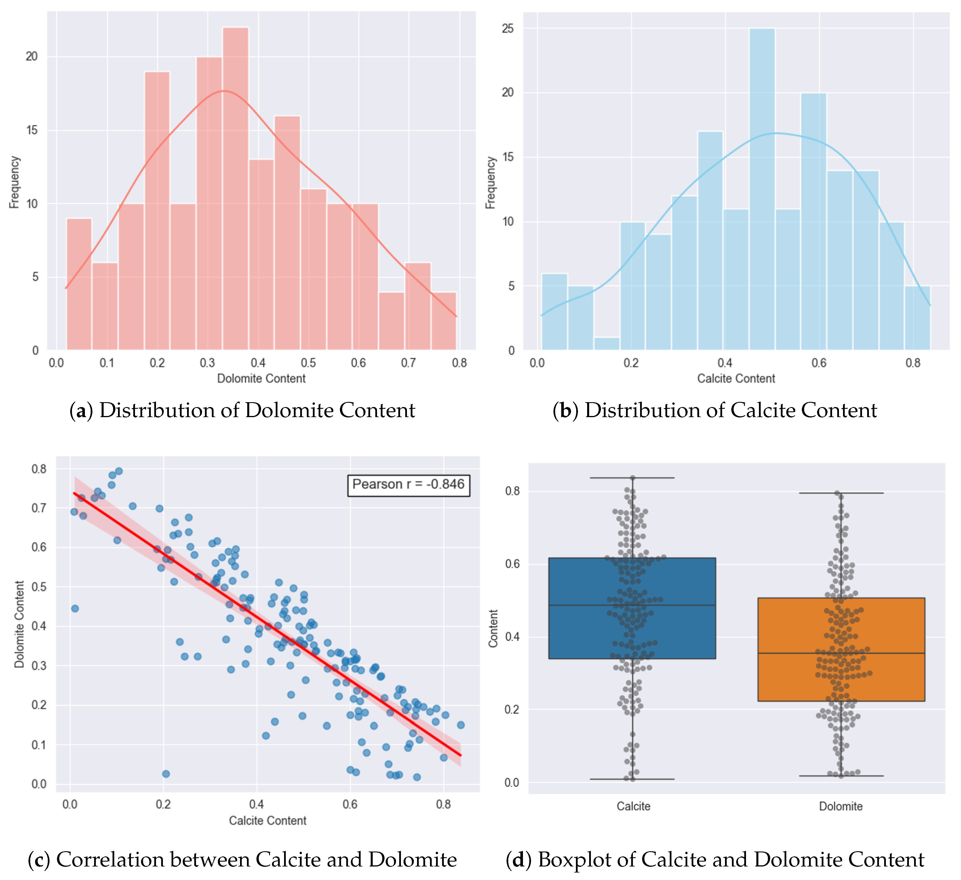
The target variables in this study are the dolomite and calcite contents, obtained via X-ray diffraction. A total of 170 distinct samples were analyzed, with calcite contents ranging from 0.01 to 0.837 and dolomite from 0.018 to 0.794, as summarized in Table 2. The mean content was 0.470 for calcite and 0.367 for dolomite, with standard deviations of 0.195 and 0.184, respectively. Both distributions are continuous, as shown in the histograms in Figure 4a,b. The distribution of dolomite tends to be more symmetric, while calcite exhibits slight positive skewness, suggesting a higher concentration of samples with elevated calcite contents. Additionally, it is worth noting that the coefficient of variation for dolomite (cv = 0.503) is higher than that of calcite (cv = 0.414), indicating greater relative dispersion of dolomite values in relation to its mean.
Table 2.
Descriptive statistics of dolomite and calcite contents in the dataset.
Figure 4.
Exploratory analysis of calcite and dolomite contents in the dataset. (a,b) show the histograms with the distribution of dolomite and calcite contents, with estimated density curves. (c) The scatter plot between calcite and dolomite contents with linear fit and Pearson correlation coefficient, indicating a strong negative correlation; (d) Boxplots comparing the distribution of calcite and dolomite contents in order to assess the presence of potential outliers.
A noteworthy point is the presence of a strong negative correlation between calcite and dolomite contents, with a Pearson coefficient of –0.846, as shown in Figure 4c. This relationship reflects a common mineralogical pattern in carbonate rocks, where the dolomitization process occurs through the substitution of calcium by magnesium in the calcite structure, resulting in the formation of dolomite [55].
Figure 4d presents boxplots accompanied by individual data points, highlighting the distribution and variability of the contents for each mineral. The median of calcite (0.487) is higher than that of dolomite (0.354), and its interquartile range is also broader, indicating greater heterogeneity. These aspects, combined with the good data dispersion and the absence of imbalance between the minerals, reinforce that the dataset is sufficiently representative and suitable for model training.
3.3. Modeling Evaluation
The performance evaluation of predictive models for the quantification of dolomite and calcite from hyperspectral signatures was conducted in multiple stages. Initially, an analysis of the hyperparameters of each method was performed, along with an evaluation of the different types of spectral transformations applied to the data. For this stage, the dataset was split into two subsets: 80% of the samples were allocated for calibration, and 20% were reserved for testing.
Using the training set, the grid search method was applied in combination with five-fold cross-validation. The best hyperparameter (Appendix A-Table A2) combinations obtained from this process were used to fit the models, which were subsequently evaluated on the test set. In this phase, the score and RMSE metrics were calculated, considering the joint prediction of dolomite and calcite concentrations.
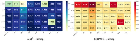
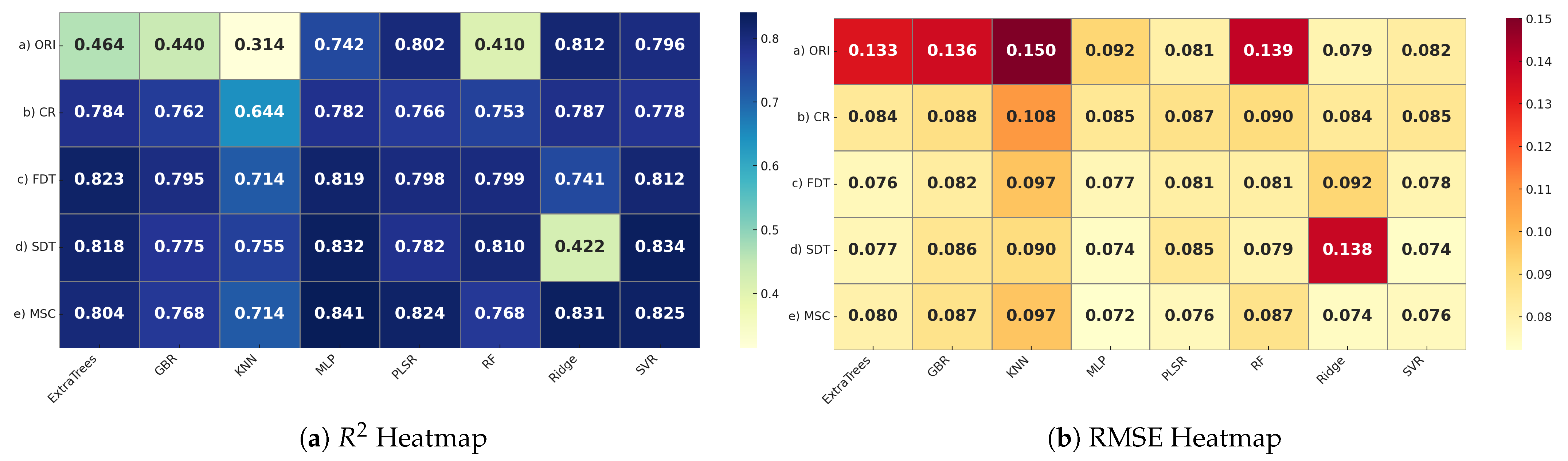
Based on the results obtained, as presented in Figure 5a,b, it is possible to observe that the performance of the models varied significantly depending on the type of spectral transformation applied and the algorithm used. Overall, ORI data showed the worst performance, especially for models based on KNN, GBR, and Ridge. In contrast, the MSC transformation yielded the best performance, with results above 76% and RMSE below 0.08.
Figure 5.
Performance of the models with different preprocessing methods for the prediction of carbonate minerals.
When comparing performance across different algorithms, it is observed that MLP and SVR yielded the best results, particularly when combined with MSC and SDT. MLP achieved a maximum of 0.841 with MSC, while SVR reached 0.834 with SDT, both with RMSE values ranging between 0.072 and 0.074. In contrast, KNN showed inferior results compared to the others. This discrepancy of results may indicate that distance-based methods are less capable of generalizing to this type of evaluated problem.
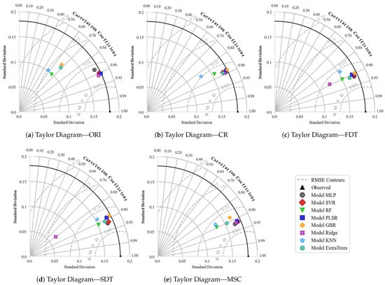
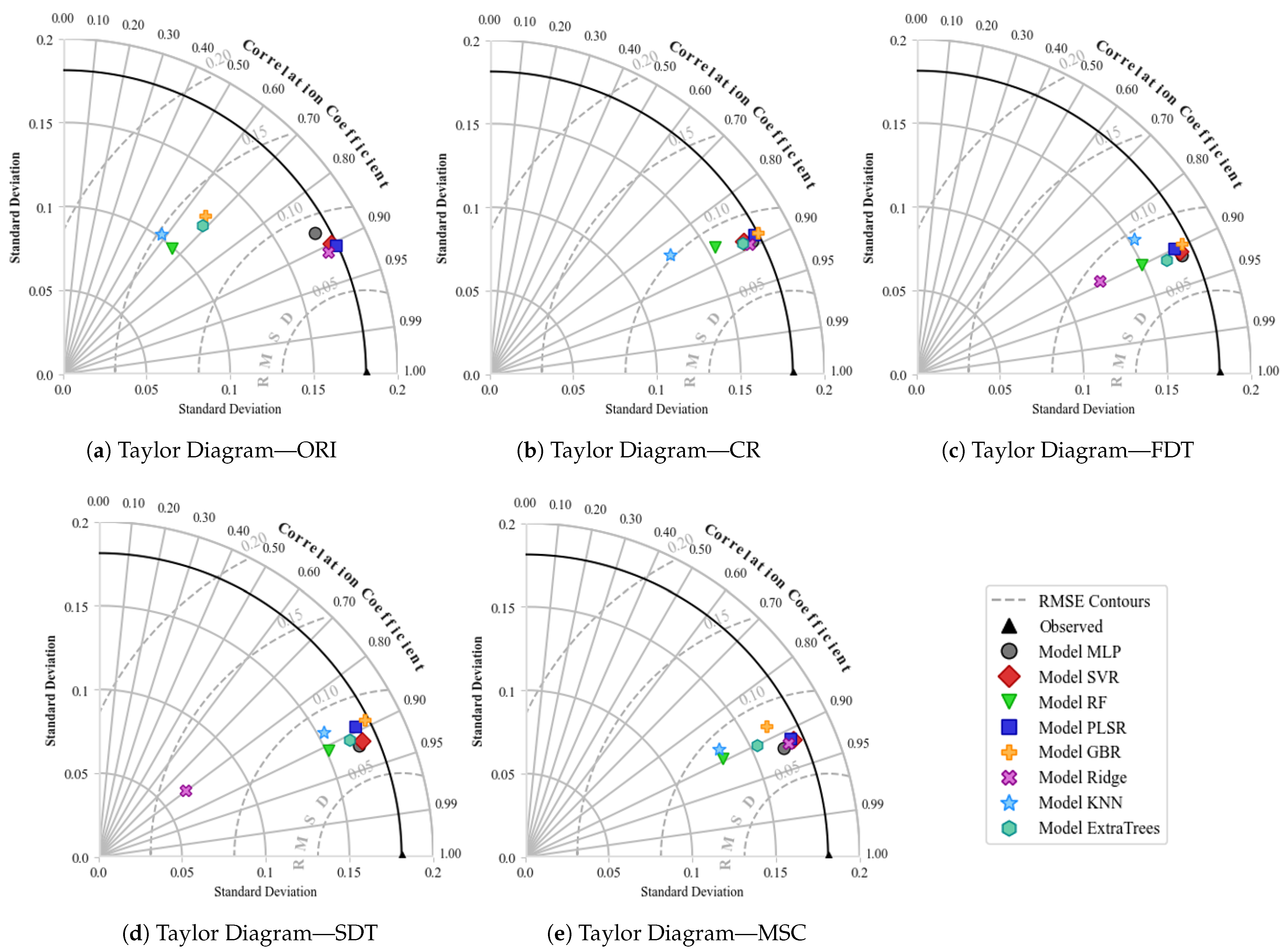
Figure 6 presents the values obtained for the different types of transformation using the Taylor Diagram. The black line highlighted in the diagrams represents the observed values, with a correlation equal to 1 and a normalized standard deviation. Each model is represented by a symbol in the diagram, and the closer this symbol is to the reference line, the better the model’s performance, as it indicates high correlation, good preservation of data variability, and reduced error.
Figure 6.
Taylor diagrams comparing the performance of regression models, combined with different spectral preprocessing methods in the joint prediction of dolomite and calcite.
When evaluating the diagrams, it is possible to observe that the combinations MSC + MLP, MLP + SDT, and MSC + SVR are located near the observed point, showing correlations close to 0.92. This indicates that the predicted variations follow the actual observed variations. The standard deviation for both remained close to the observed value, suggesting that there was neither overestimation nor underestimation. Furthermore, the reduced RMSD indicates that, even when errors occur, they are small and randomly distributed.
Other combinations, such as SDT + SVR and MSC + Ridge, also stood out; however, both presented RMSD and standard deviation values slightly lower than the previously highlighted combinations. This difference indicates that these combinations resulted in lower variability in the predictions, which may represent a possible loss in the ability to capture more subtle variations present in the original data.
Based on the joint interpretation of the heatmaps and Taylor Diagrams, it was possible to identify the combinations that best balance performance and stability. Table 3 presents the five best combinations, along with the values of the respective performance metrics obtained. Despite the good results, it was still not statistically possible to determine which of these combinations performs best. To address this issue, the Friedman and Nemenyi statistical tests were applied. The Friedman test was used to verify whether the observed performance differences are statistically significant, while the Nemenyi post hoc test allowed the identification of which combinations present significant performance differences, based on a predefined confidence level.
Table 3.
Performance of the five best combinations on the test set.
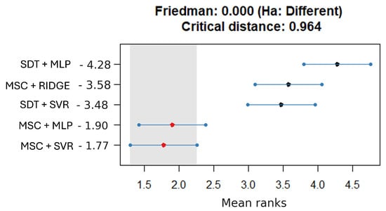
For the application of statistical tests, each of the five selected combinations has been executed 40 times, altering only the random seed used in the train-test split. This variation resulted in a set of 40 values in the test set (Appendix A - Table A1), which were used as input for the Friedman and Nemenyi tests. Figure 7 presents the average rank of each combination, considering a 95% confidence level.
Figure 7.
Statistical comparison using the Friedman and Nemenyi methods for identifying the best combination in the prediction of dolomite and calcite.
Based on Figure 7, the average ranks of each combination are shown in descending order, from the best to the worst performance. Analyzing the results, the Friedman test indicated that there are significant differences between the techniques evaluated. In the Nemenyi test, it is observed that MSC + SVR, with an average rank of 1.77, and MSC + MLP, with 1.90, presented the lowest values. The difference between these ranks is smaller than the calculated CD of 0.964, indicating, with a 95% confidence level, that the performance between these two combinations is not statistically different.
On the other hand, the combinations SDT + MLP (4.28), MSC + Ridge (3.58), and SDT + SVR (3.48) show considerably higher average ranks. Comparing the first two, the difference between the values exceeds the calculated CD, demonstrating that these combinations are statistically inferior. Thus, with 95% confidence, it is concluded, based on the Friedman and Nemenyi tests, that the combinations MSC + SVR and MSC + MLP are the most effective for predicting dolomite and calcite compared to the other combinations evaluated.
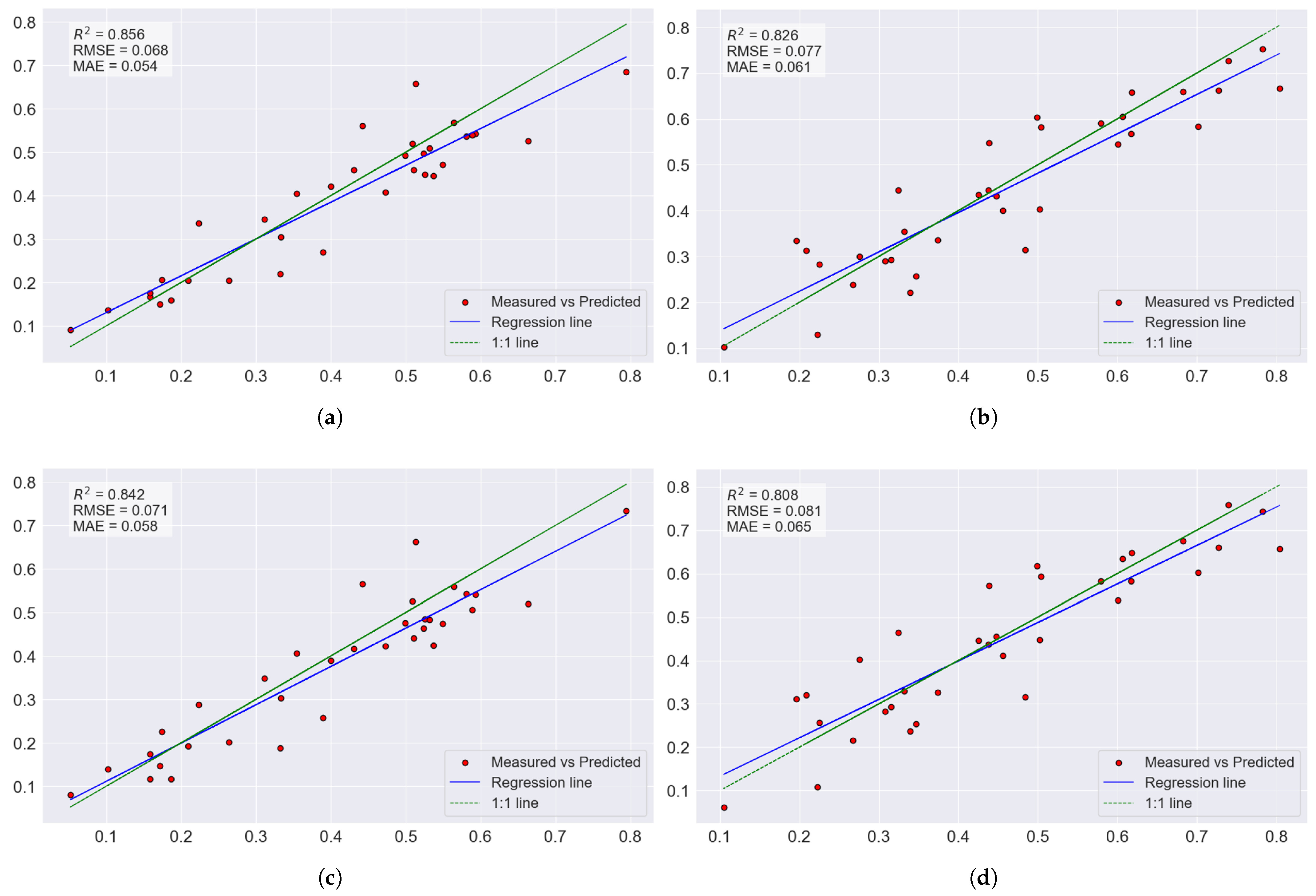
In order to separately evaluate the models’ performance for each mineral, Figure 8 shows the relationship between measured and predicted values for dolomite and calcite using the MSC + MLP and MSC + SVR combinations, respectively. The analysis indicates that there were no relevant discrepancies between the mineral predictions, suggesting consistent model behavior in both cases. The slightly superior performance observed for dolomite may be attributed to its higher coefficient of variation (Table 2), which tends to favor statistical fitting. Nevertheless, this difference is not significant, reinforcing that the evaluated combinations maintain a strong ability to predict the minerals within the studied context.
Figure 8.
Relationship between measured and predicted values for dolomite and calcite using the MLP + MSC and SVR + MSC combinations. The diagonal lines represent the ideal (1:1) correspondence between observed and estimated values. (a) Regression plot for dolomite content MSC + MLP. (b) Regression plot for calcite content MSC + MLP. (c) Regression plot for dolomite content MSC + SVR. (d) Regression plot for calcite content MSC + SVR.
3.4. Explanation of the Best Model Combinations
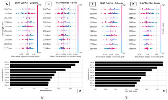
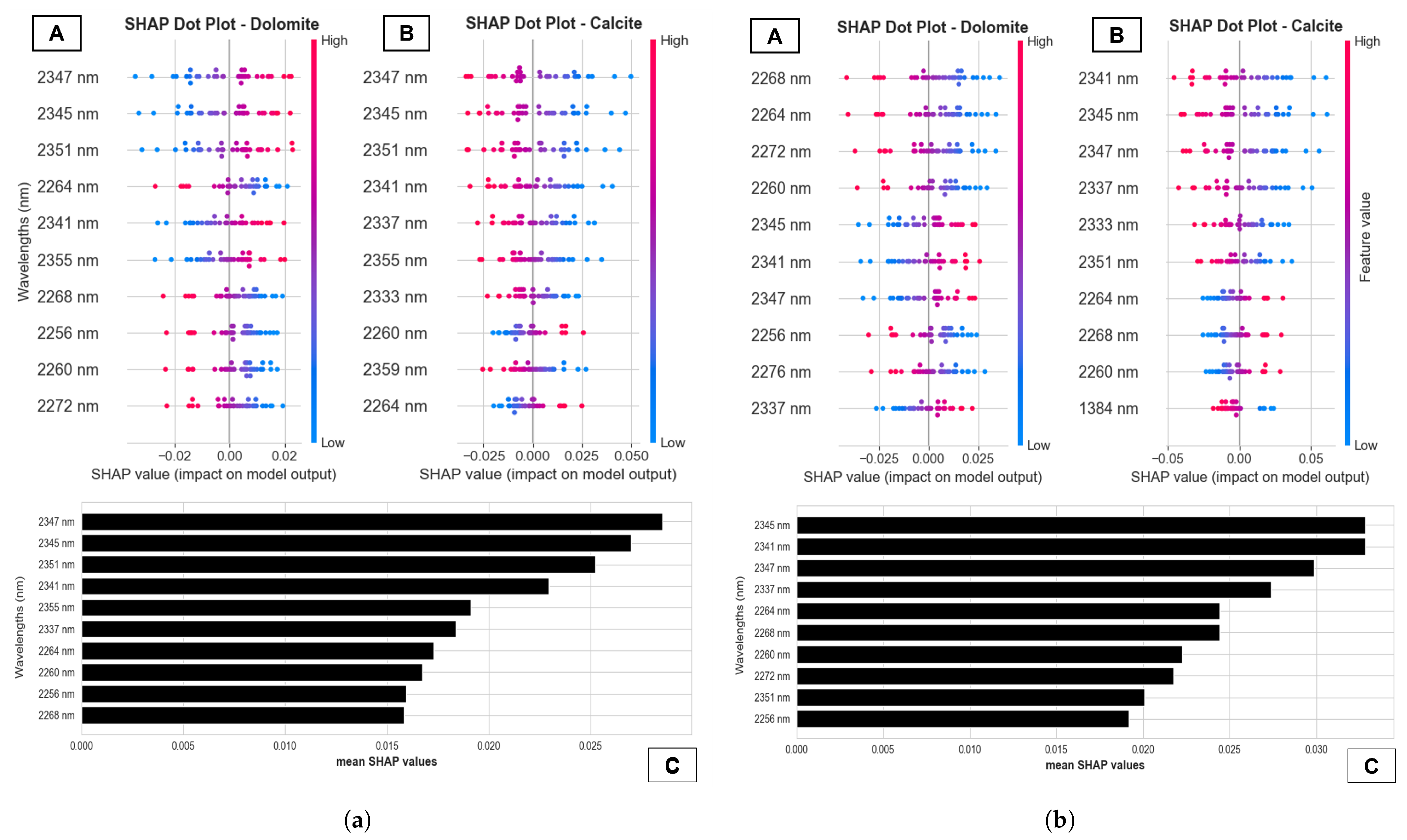
After identifying the best combinations for quantifying the evaluated minerals, the explainability analysis of these best-performing combinations was carried out using the SHAP technique applied to the test set. In general, the results presented in Figure 9 highlight that the bands located in the 2330–2360 nm interval exerted the most significant impact. This was an expected result, since these wavelengths are directly associated with the characteristic absorptions of the carbonate group .
Figure 9.
SHAP-based interpretation for the best combinations. In each column, (A,B) show SHAP summary (beeswarm) plots for dolomite and calcite on the test set. C presents the bar chart with the 10 bands with the highest global importance (mean |SHAP|). The horizontal axis represents the SHAP value, where positive values increase, and negative values decrease the estimated mineral concentration. The colors indicate the reflectance value of the feature (low = blue; high = magenta). (a) SHAP feature importance plots for interpreting the MSC + MLP. (b) SHAP feature importance plots for interpreting the MSC + SVR.
Figure 9a illustrates the explainability results obtained for the MSC+MLP combination. It can be observed that the explanatory patterns for dolomite and calcite are inversely related, as evidenced in the beeswarm plots. For instance, in the case of dolomite, the cluster of blue-colored points located on the negative side for the 2347 nm wavelength indicates that low reflectance values result in equally low SHAP values, contributing to the prediction of lower dolomite concentrations. In contrast, for calcite, the same spectral range (2347 nm) exhibits the opposite behavior: reduced reflectance values are associated with higher positive SHAP contributions, supporting the estimation of higher calcite concentrations.
In the case of the MSC+SVR combination, the explainability results maintain the inverse relationship previously observed. However, as shown in Figure 9b, for dolomite, the wavelengths between 2260 and 2280 nm stood out with the greatest impact. This spectral region is associated with clay minerals but may also reflect carbonate interactions, depending on the chemical composition and crystal structure of the sample [5]. For calcite, the pattern observed in the MSC + MLP result was reproduced again, reinforcing the consistency across different preprocessing and model combinations.
Finally, the analysis of the bar plots in Figure 9a,b, which represent the combined average influence of the variables for both minerals, reveals a convergence in the results. Wavelengths such as 2341 nm, 2345 nm, 2347 nm, 2260 nm, 2264 nm, and 2268 nm appear among the most influential. This recurrence suggests that these spectral regions constitute critical points for the discrimination and quantification of both minerals, regardless of the combination evaluated.
3.5. Prediction Maps of the Drill Core
Based on the dolomite and calcite quantification models that showed the best performance (as evaluated in Section 3.3), concentrations of these minerals were predicted in hyperspectral images of drill core samples. The primary goal of this step was to visualize the spatial distribution of those minerals along the core, followed by a comparison of these predictions with the XRF data for Ca and Mg.
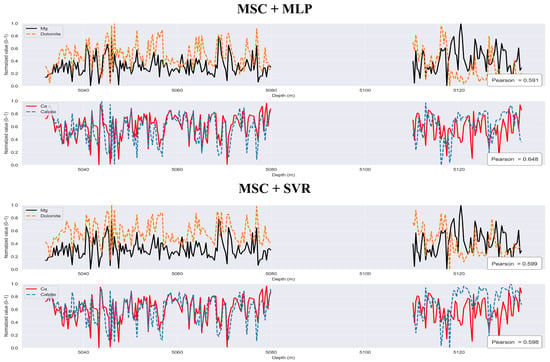
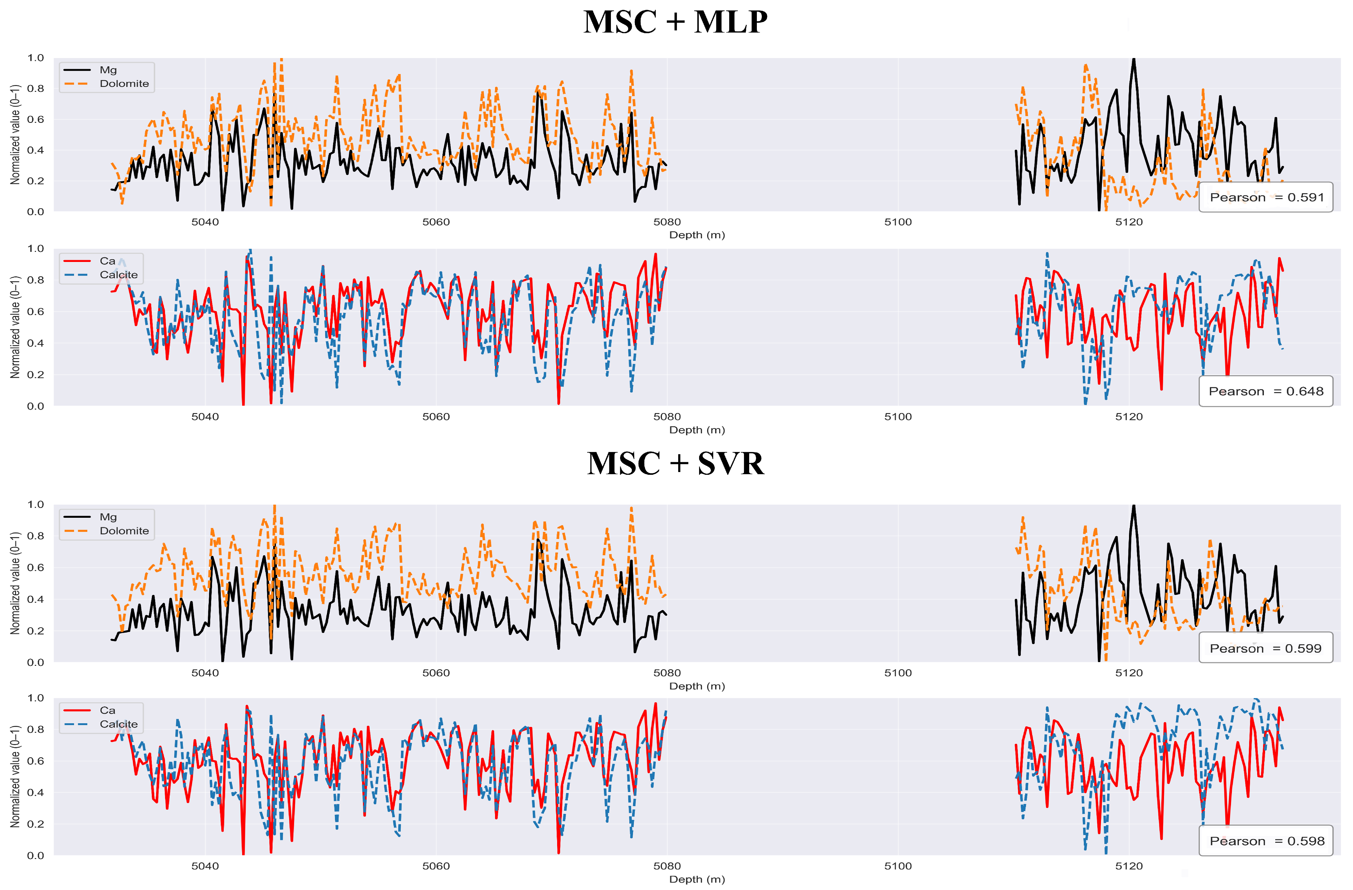
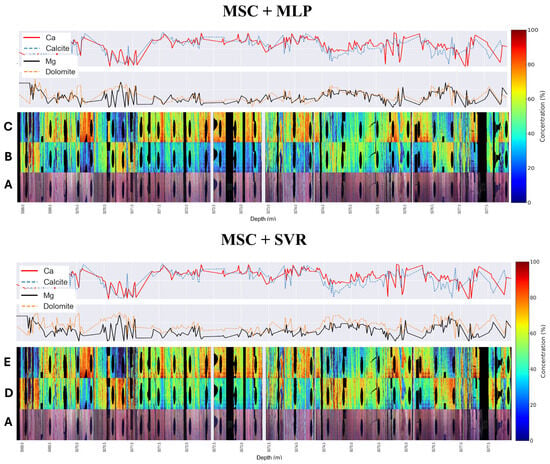
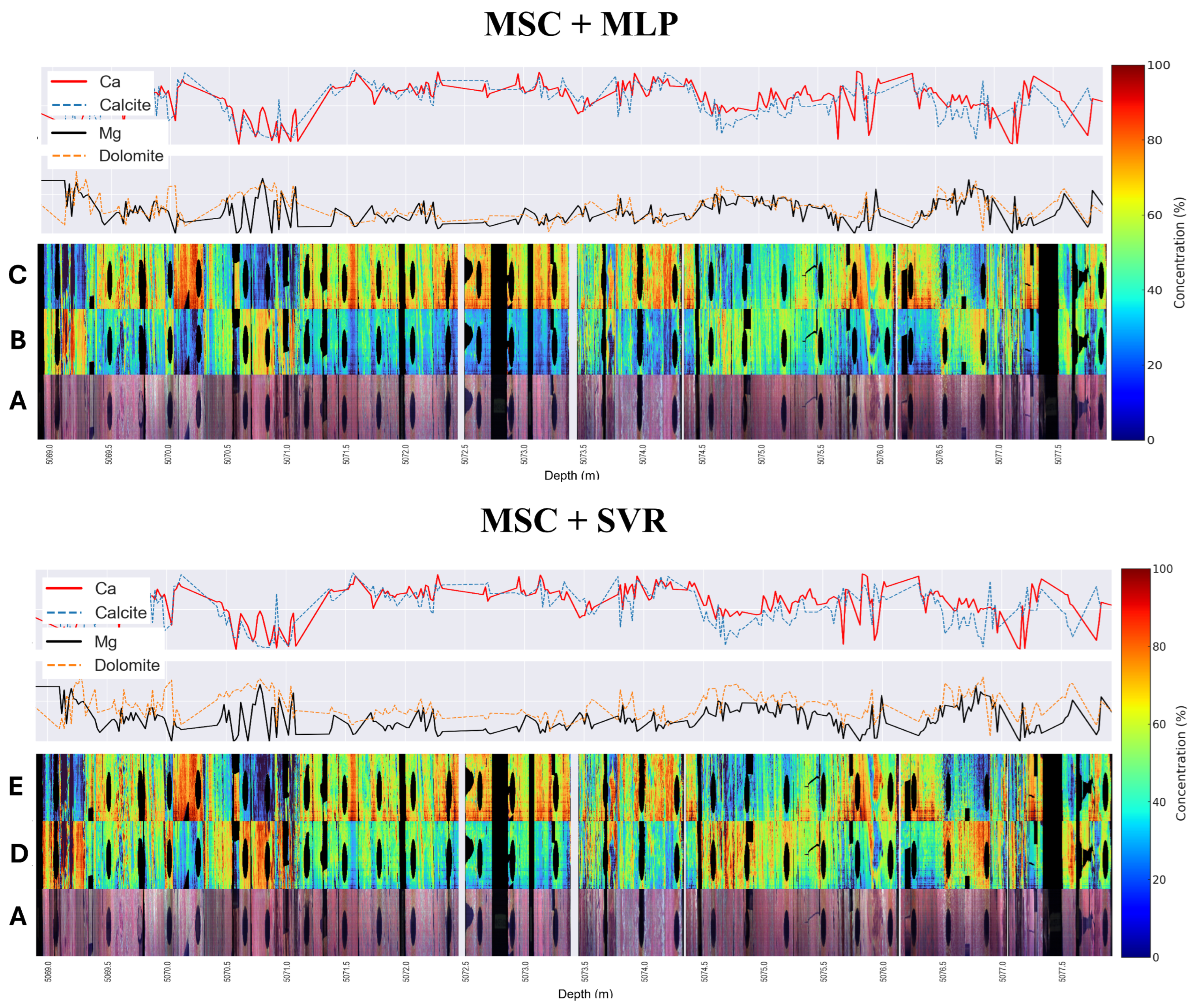
Figure 10 and Figure 11 present a comparison between the predictions of dolomite and calcite and the Ca and Mg concentration profiles obtained by XRF along the core. Figure 10 illustrates the profiles comparison for all evaluated core samples. It was observed that, for both model combinations, the Pearson correlation between predicted concentrations of dolomite and calcite and the respective Mg and Ca measurements was approximately 60%.
Figure 10.
Comparison between predicted mineral concentration profiles and geochemical data obtained via X-ray fluorescence (XRF). The plots display the depth-registered distribution of dolomite and calcite for all evaluated core samples, showing a Pearson correlation of approximately 60% between the hyperspectral estimates and the Mg and Ca measurements.
Figure 11.
Detailed analysis of a selected drill core section showing the spatial correspondence between mineral prediction maps and XRF profiles. (A) RGB composite of the core. (B,D) Prediction maps for dolomite and (C,E) calcite using the best-performing model combinations. Warm colors indicate higher concentrations, aligning with Mg and Ca peaks in the geochemical profiles.
For a more detailed and quantitative analysis, a specific section of the core was selected, as outlined in Figure 11. In this section, a clear qualitative correspondence was observed between the hyperspectral images and the XRF data. Regions characterized by high calcite concentrations (warm colors on prediction maps C and E) consistently align with Ca peaks in the XRF profiles. Similarly, areas rich in dolomite on prediction maps B and D correlate with Mg peaks and, inversely, with lower Ca concentrations, reinforcing the validity of predictions.
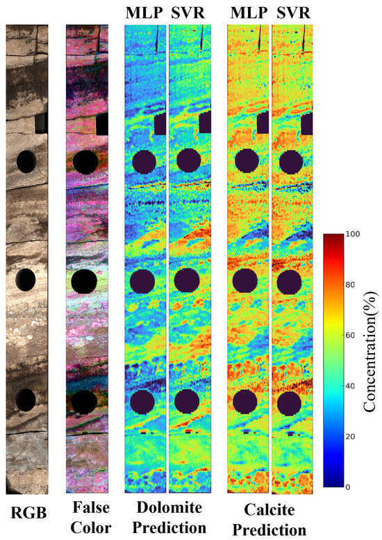
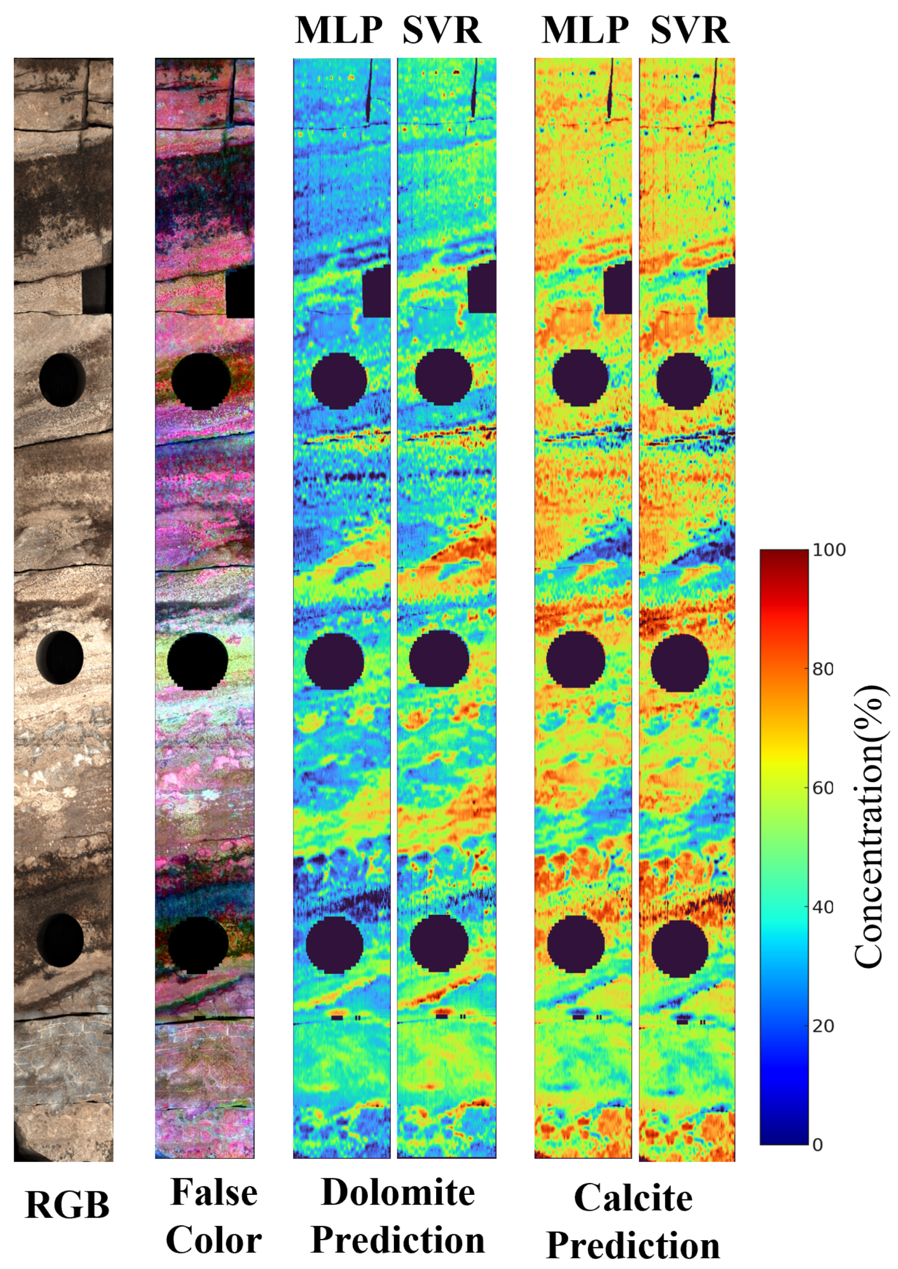
Figure 12 presents a detailed view of the mineral prediction results for a single drill core. Image analysis allows for the identification of both commonalities and visual differences between the two best model combinations. In both cases, the ability to consistently capture the spatial variation in the minerals is evident, respecting transitions across different mineralogical regions. However, some subtle distinctions can be observed. The MSC+MLP model tends to produce smoother color transitions, resulting in predictions with less noise. In contrast, the MSC+SVR model displays slightly sharper boundaries and more pronounced color intensity variations, suggesting higher sensitivity. Despite these differences, both models demonstrate consistent mineralogical prediction performance throughout the core.
Figure 12.
Representation of the spatial distribution of dolomite and calcite predictions based on the best evaluated model combinations.
4. Discussion
Quantification of carbonate minerals in drill cores through the combination of HSI and ML algorithms is an evolving research area with direct implications for reservoir characterization and mineral exploration. The results obtained in this study demonstrate the effectiveness of a methodological approach that integrates spectral preprocessing optimization, nonlinear predictive algorithms, and rigorous statistical validation. The combination involving MSC preprocessing with the MLP and SVR algorithms yielded the best overall performance in terms of accuracy ( and RMSE) and stability. These findings reinforce the premise that predictive performance depends strongly on the optimization of the processing chain, rather than solely on the choice of algorithm.
An important methodological contribution of this work is the development of an integrated workflow that harmonizes continuous hyperspectral data acquisition with point-based mineralogical validation from complementary sensors (XRF and XRD). This operational synergy helps reduce the gap between the high spatial resolution of HSI and the analytical rigor of conventional laboratory techniques, establishing a robust calibration protocol for carbonate quantification.
The results also reinforce previous findings in the literature, particularly regarding the importance of preprocessing and spectral feature selection for quantitative modeling. The study by Wei et al. (2024) [17] proposed a hybrid method combining spectral knowledge and ML to estimate dolomite content in outcrops, highlighting the relevance of incorporating geological criteria into predictive workflows. The present study complements this perspective by systematically demonstrating that the choice of preprocessing methods can be decisive for model performance and that such optimization should be verified through statistical testing. The use of the non-parametric Friedman and Nemenyi tests allowed assessment of whether the observed differences among the best-performing combinations were statistically significant, adding an objective criterion for comparing methods and reducing conclusions based solely on sampling variation.
In the context of predictive modeling, the superior performance of nonlinear and ensemble algorithms (such as Random Forest and MLP) compared with linear models (such as PLSR and Ridge Regression) is consistent with findings reported in recent studies [14,15]. Previous works, such as Zaini et al. (2014) [13], had already indicated the potential of HSI, although under simpler analytical approaches. The relationship between reflectance and mineral concentration may be complex due to mixing effects, scattering, and nonlinear spectral interactions, which favor models capable of capturing nonlinear responses. In this regard, the results obtained for calcite and dolomite in pre-salt cores fall within a range comparable to that reported in similar studies conducted in other geological settings [14,15], suggesting that the evaluated workflow is suitable for carbonate environments with greater geological complexity.
A central aspect of this work is the incorporation of interpretability through XAI techniques. While many studies prioritize predictive performance and scalability, the geological explanation of what the model is using is not always explicitly addressed. Herein, the application of SHAP enabled variable-importance analysis and indicated that the model relies on spectral features associated with carbonates, particularly the region around 2330–2360 nm, for quantification. This is relevant because it establishes a direct link between the model response and the expected diagnostic spectral features of carbonate minerals, helping to verify whether the prediction is geologically meaningful. By discussing the model contributions based on physicochemical principles, this work reduces reliance on a purely “black-box” interpretation and provides a more transparent pathway for validating model behavior in geological applications.
Despite the proposed workflow and the results obtained, some limitations should be considered. Validation based on XRD in discrete samples (plugs) may introduce a scale mismatch relative to the continuous HSI data, which can affect direct comparisons between estimates and references. Future studies may explore integration with X-ray microtomography for volumetric validation. Moreover, the focus on calcite and dolomite, although justified by the low quartz concentration in the evaluated samples, limits generalization to scenarios with more diverse mineralogy. A natural step for future expansion is the inclusion of other relevant minerals, such as clays and sulfides, which may interfere in the SWIR region and modify the observed spectral response.
Future developments should converge toward generalization and data integration. The evaluation of Domain Adaptation and Transfer Learning techniques may help test the application of these models in other pre-salt fields or different carbonate reservoirs, reducing the cost and time associated with building new calibration datasets. Expanding the XAI analysis with methods that provide local explanations may offer additional insights into spatial variations and mineralogical heterogeneity. Finally, integrating hyperspectral quantification with geophysical and petrophysical log data represents an important step toward bringing mineralogical estimates closer to reservoir interpretation and decision-making workflows.
5. Conclusions
This study demonstrated that the integration of hyperspectral imaging and Machine Learning provides an effective and interpretable approach for the quantification of carbonates (calcite and dolomite) in pre-salt drill cores. The evaluated workflow achieved high predictive accuracy and enabled continuous high-resolution mineralogical profiling, representing an important advancement over traditional destructive and point-based methods.
A critical distinguishing feature of this work lies in the application of eXplainable Artificial Intelligence (XAI) methods. By unveiling the “black-box” of Machine-Learning models, we were able to establish a direct correlation between diagnostic spectral features of carbonates and the model predictions. This interpretability is essential for geological validation of the results and for building confidence in the application of these technologies in complex environments. The ability to trace spectral contributions to mineral quantification not only reinforces the scientific robustness of the approach but also provides valuable insights into the understanding of geological processes.
The results obtained, supported by X-ray diffraction (XRD) and X-ray fluorescence (XRF) data, provide a powerful tool for the detailed characterization of carbonate reservoirs, directly impacting the assessment of porosity, permeability, and reservoir quality. This work not only fills a gap in the literature by offering a systematic evaluation of robustness and interpretability but also establishes a protocol for the efficient implementation of hyperspectral core logging routines. The practical implications extend to the optimization of natural resource exploration and management, contributing to informed and sustainable decision-making in the oil and gas industry.
For future research, it is recommended to explore the generalization of these models for different sedimentary basins and carbonate rock types, as well as their integration with other geophysical and geological data sources for more comprehensive reservoir characterization. The continuous evolution of Machine-Learning and Remote-Sensing techniques promises to further enhance the ability to unravel the complexity of geological systems, driving innovation in mineral exploration.
Author Contributions
Conceptualization, V.S. and M.V.; Methodology, V.S., G.R. and L.S.; Software, V.S. and L.S.; Validation, V.S., G.R., L.S., A.A., J.L., R.S., L.d.S., R.D., D.M., A.M., D.Z., D.I., L.G.J. and M.V.; Formal Analysis, V.S., G.R. and L.S.; Investigation, V.S., G.R., L.S., A.A., J.L., R.S., L.d.S., R.D. and D.M.; Resources, A.M., D.I. and M.V.; Data Curation, V.S. and G.R.; Writing—Original Draft Preparation, V.S.; Writing—Review and Editing, V.S., G.R., M.V., D.Z. and D.I.; Visualization, V.S. and L.S.; Supervision, M.V. and D.I.; Project Administration, M.V. and D.I.; Funding Acquisition, M.V. and D.I. All authors have read and agreed to the published version of the manuscript.
Funding
This research was funded by Petróleo Brasileiro S.A. (PETROBRAS), grant number 4600556376; Agência Nacional do Petróleo, Gás Natural e Biocombustíveis (ANP), grant number 4600583791; and Coordenação de Aperfeiçoamento de Pessoal de Nível Superior (CAPES), grant number 001. The APC was funded by CAPES.
Data Availability Statement
The data presented in this study are available on request from the corresponding author. The data are not publicly available due to confidentiality agreements with Petrobras and the proprietary nature of the hyperspectral and XRD datasets from the pre-salt carbonate reservoirs.
Acknowledgments
The authors acknowledge the Vizlab|X-Reality and Geoinformatics Lab at UNISINOS University for providing computational resources and infrastructure. We thank the Petrobras Research and Development Center (CENPES) for access to the drill core samples and analytical facilities. Special thanks to the technical team at CENPES for their support in data acquisition and sample preparation. The authors also acknowledge the use of the SPECCAM 4 hyperspectral sensor and the Vanta Max X-ray fluorescence equipment for data collection.
Conflicts of Interest
The authors declare no conflicts of interest. The funders (PETROBRAS, ANP, and CAPES) had no role in the design of the study; in the collection, analyses, or interpretation of data; in the writing of the manuscript, or in the decision to publish the results.
Abbreviations
The following abbreviations are used in this manuscript:
| ANN | Artificial Neural Networks |
| CD | Critical Difference |
| CR | Continuum Removal |
| FDT | First Derivative Transformation |
| FWHM | Full Width at Half Maximum |
| GBR | Gradient Boosting Regressor |
| HSI | Hyperspectral Imaging |
| KNN | K-Nearest Neighbors |
| LSU | Linear Spectral Unmixing |
| ML | Machine Learning |
| MLP | Multi-Layer Perceptron |
| MSC | Multiplicative Scatter Correction |
| MSCL | Multi-Sensor Core Logger |
| ORI | Original Spectra |
| PLSR | Partial Least Squares Regression |
| RF | Random Forest |
| RMSD | Root Mean Square Difference |
| RMSE | Root Mean Square Error |
| SAM | Spectral Angle Mapper |
| SDT | Second Derivative Transformation |
| SHAP | SHapley Additive exPlanations |
| SVR | Support Vector Regression |
| SWIR | Shortwave Infrared |
| TIR | Thermal Infrared |
| XAI | eXplainable Artificial Intelligence |
| XRD | X-ray Diffraction |
| XRF | X-ray Fluorescence |
Appendix A
This appendix presents the 40 results obtained for each of the five selected model combinations. Each run corresponds to a distinct variation in the random seed used in the training and testing data split, resulting in a set of 40 values on the test set. These values served as the basis for applying the Friedman and Nemenyi statistical tests.
Table 2 presents the best hyperparameters for each combination of Machine-Learning model and spectral preprocessing. The selection of these parameters was carried out through a grid search analysis with 5-fold cross-validation.
Table A1.
Test values for 40 runs across the five model combinations.
Table A2.
Optimized hyperparameters for each model and preprocessing type.
References
- Lucia, F.J. Carbonate Reservoir Characterization: An Integrated Approach; Springer: Berlin, Germany, 2014. [Google Scholar]
- Warren, J. Dolomite: Occurrence, evolution and economically important associations. Earth-Sci. Rev. 2000, 52, 1–81. [Google Scholar] [CrossRef] [Scilit]
- Środoń, J. Identification and quantitative analysis of clay minerals. Dev. Clay Sci. 2013, 5, 25–49. [Google Scholar]
- Hillier, S. Accurate quantitative analysis of clay and other minerals in sandstones by XRD: Comparison of a Rietveld and a reference intensity ratio (RIR) method and the importance of sample preparation. Clay Miner. 2000, 35, 291–302. [Google Scholar] [CrossRef] [Scilit]
- Clark, R.N.; Swayze, G.A.; Livo, K.E.; Kokaly, R.F.; Sutley, S.J.; Dalton, J.B.; McDougal, R.R.; Gent, C.A. Imaging spectroscopy: Earth and planetary remote sensing with the USGS Tetracorder and expert systems. J. Geophys. Res. Planets 2003, 108, 5131. [Google Scholar] [CrossRef] [Scilit]
- van der Meer, F.D.; van der Werff, H.M.; van Ruitenbeek, F.J.; Hecker, C.A.; Bakker, W.H.; Noomen, M.F.; van der Meijde, M.; Carranza, E.J.M.; de Smeth, J.B.; Woldai, T. Multi- and hyperspectral geologic remote sensing: A review. Int. J. Appl. Earth Obs. Geoinf. 2012, 14, 112–128. [Google Scholar] [CrossRef] [Scilit]
- Clark, R.N.; King, T.V.; Klejwa, M.; Swayze, G.A.; Vergo, N. High spectral resolution reflectance spectroscopy of minerals. J. Geophys. Res. Solid Earth 1990, 95, 12653–12680. [Google Scholar]
- Hunt, G.R.; Ashley, R.P. Spectra of altered rocks in the visible and near infrared. Econ. Geol. 1979, 74, 1613–1629. [Google Scholar] [CrossRef] [Scilit]
- de Freitas, V.A.; dos Santos Vital, J.C.; Rodrigues, B.R.; Rodrigues, R. Source rock potential, main depocenters, and CO2 occurrence in the pre-salt section of Santos Basin, southeast Brazil. J. South Am. Earth Sci. 2022, 115, 103760. [Google Scholar] [CrossRef] [Scilit]
- Contreras Acosta, I.C.; Khodadadzadeh, M.; Gloaguen, R. Resolution enhancement for drill-core hyperspectral mineral mapping. Remote Sens. 2021, 13, 2296. [Google Scholar] [CrossRef] [Scilit]
- Gairola, G.S.; Thiele, S.T.; Khanna, P.; Ramdani, A.; Gloaguen, R.; Vahrenkamp, V. A data-driven hyperspectral method for sampling of diagenetic carbonate fabrics–A case study using an outcrop analogue of Jurassic Arab-D reservoirs, Saudi Arabia. Mar. Pet. Geol. 2024, 161, 106691. [Google Scholar]
- Thiele, S.T.; Kirsch, M.; Lorenz, S.; Saffi, H.; El Alami, S.; Contreras Acosta, I.C.; Madriz, Y.; Gloaguen, R. Maximising the value of hyperspectral drill core scanning through real-time processing and analysis. Front. Earth Sci. 2024, 12, 1433662. [Google Scholar] [CrossRef] [Scilit]
- Zaini, N.; Van der Meer, F.; Van der Werff, H. Effect of grain size and mineral mixing on carbonate absorption features in the SWIR and TIR wavelength regions. Remote Sens. 2012, 4, 987–1003. [Google Scholar] [CrossRef] [Scilit]
- Zaini, N.; Van der Meer, F.; Van der Werff, H. Determination of carbonate rock chemistry using laboratory-based hyperspectral imagery. Remote Sens. 2014, 6, 4149–4172. [Google Scholar] [CrossRef] [Scilit]
- Tuşa, L.; Khodadadzadeh, M.; Contreras, C.; Rafiezadeh Shahi, K.; Fuchs, M.; Gloaguen, R.; Gutzmer, J. Drill-core mineral abundance estimation using hyperspectral and high-resolution mineralogical data. Remote Sens. 2020, 12, 1218. [Google Scholar] [CrossRef] [Scilit]
- De la Rosa, R.; Khodadadzadeh, M.; Tusa, L.; Kirsch, M.; Gisbert, G.; Tornos, F.; Tolosana-Delgado, R.; Gloaguen, R. Mineral quantification at deposit scale using drill-core hyperspectral data: A case study in the Iberian Pyrite Belt. Ore Geol. Rev. 2021, 139, 104514. [Google Scholar] [CrossRef] [Scilit]
- Wei, W.; Shao, Y.; Hu, Z.; Wang, Q.; Deng, F.; Huang, Y.; Zhao, K. Estimation of the dolomite content of carbonate rock outcrops based on spectral knowledge and machine learning. Front. Earth Sci. 2024, 12, 1401026. [Google Scholar] [CrossRef] [Scilit]
- Shreeve, J.W. The use of a multi-sensor core scanner workflow as the backbone of a digital core repository. Geol. Soc. 2023, 527, 59–76. [Google Scholar] [CrossRef] [Scilit]
- Kruse, F.; Lefkoff, A.; Boardman, J.; Heidebrecht, K.; Shapiro, A.; Barloon, P.; Goetz, A. The spectral image processing system (SIPS)—interactive visualization and analysis of imaging spectrometer data. Remote Sens. Environ. 1993, 44, 145–163. [Google Scholar] [CrossRef] [Scilit]
- Badola, A.; Panda, S.K.; Roberts, D.A.; Waigl, C.F.; Bhatt, U.S.; Smith, C.W.; Jandt, R.R. Hyperspectral data simulation (sentinel-2 to aviris-ng) for improved wildfire fuel mapping, Boreal Alaska. Remote Sens. 2021, 13, 1693. [Google Scholar] [CrossRef] [Scilit]
- Schläpfer, D.; Boerner, A.; Schaepman, M. The Potential of Spectral Resampling Techniques for the Simulation of APEX Imagery Based on AVIRIS Data. In Proceedings of the AVIRIS Workshop, Pasadena, CA, USA, 10–11 February 1999. [Google Scholar]
- Kalopesa, E.; Karyotis, K.; Tziolas, N.; Tsakiridis, N.; Samarinas, N.; Zalidis, G. Estimation of sugar content in wine grapes via in situ VNIR–SWIR point spectroscopy using explainable artificial intelligence techniques. Sensors 2023, 23, 1065. [Google Scholar] [CrossRef] [Scilit] [PubMed]
- Ahmed, M.T.; Villordon, A.; Kamruzzaman, M. Hyperspectral imaging and explainable deep-learning for non-destructive quality prediction of sweetpotato. Postharvest Biol. Technol. 2025, 222, 113379. [Google Scholar] [CrossRef] [Scilit]
- Lin, N.; Jiang, R.; Li, G.; Yang, Q.; Li, D.; Yang, X. Estimating the heavy metal contents in farmland soil from hyperspectral images based on Stacked AdaBoost ensemble learning. Ecol. Indic. 2022, 143, 109330. [Google Scholar] [CrossRef] [Scilit]
- Zhou, W.; Yang, H.; Xie, L.; Li, H.; Huang, L.; Zhao, Y.; Yue, T. Hyperspectral inversion of soil heavy metals in Three-River Source Region based on random forest model. CATENA 2021, 202, 105222. [Google Scholar] [CrossRef] [Scilit]
- Ma, X.; Wang, J.; Zhou, K.; Zhang, W.; Zhang, Z.; Zhou, S.; Bai, Y.; De Maeyer, P.; Van de Voorde, T. Quantitative evaluation of the impact of band optimization methods on the accuracy of the hyperspectral metal element inversion models. Int. J. Appl. Earth Obs. Geoinf. 2024, 132, 104011. [Google Scholar] [CrossRef] [Scilit]
- Zhang, S.; Shen, Q.; Nie, C.; Huang, Y.; Wang, J.; Hu, Q.; Ding, X.; Zhou, Y.; Chen, Y. Hyperspectral inversion of heavy metal content in reclaimed soil from a mining wasteland based on different spectral transformation and modeling methods. Spectrochim. Acta Part A Mol. Biomol. Spectrosc. 2019, 211, 393–400. [Google Scholar] [CrossRef] [Scilit]
- Rinnan, Åsmund; van den Berg, F.; Engelsen, S.B. Review of the most common pre-processing techniques for near-infrared spectra. TrAC. Trends Anal. Chem. 2009, 28, 1201–1222. [Google Scholar] [CrossRef] [Scilit]
- Wold, S.; Sjöström, M.; Eriksson, L. PLS-regression: A basic tool of chemometrics. Chemom. Intell. Lab. Syst. 2001, 58, 109–130. [Google Scholar] [CrossRef] [Scilit]
- Nawar, S.; Buddenbaum, H.; Hill, J.; Kozak, J.; Mouazen, A.M. Estimating the soil clay content and organic matter by means of different calibration methods of vis-NIR diffuse reflectance spectroscopy. Soil Tillage Res. 2016, 155, 510–522. [Google Scholar] [CrossRef] [Scilit]
- Ma, X.; Wang, J.; Zhou, K.; Zhang, W.; Zhang, Z.; De Maeyer, P.; Van de Voorde, T. New data-driven estimation of metal element in rocks using a hyperspectral data and geochemical data. Ore Geol. Rev. 2024, 165, 105877. [Google Scholar] [CrossRef] [Scilit]
- Hoerl, R.W. Ridge regression: A historical context. Technometrics 2020, 62, 420–425. [Google Scholar] [CrossRef] [Scilit]
- McDonald, G.C. Ridge regression. Wiley Interdiscip. Rev. Comput. Stat. 2009, 1, 93–100. [Google Scholar] [CrossRef] [Scilit]
- Drucker, H.; Burges, C.J.; Kaufman, L.; Smola, A.; Vapnik, V. Support vector regression machines. In Proceedings of the Advances in Neural Information Processing Systems 9 (NIPS1996), Denver, CO, USA, 2–5 December 1996. [Google Scholar]
- Awad, M.; Khanna, R. Support vector regression. In Efficient Learning Machines: Theories, Concepts, and Applications for Engineers and System Designers; Apress: Berkeley, CA, USA, 2015; pp. 67–80. [Google Scholar]
- Wang, L.; Kisi, O.; Zounemat-Kermani, M.; Salazar, G.A.; Zhu, Z.; Gong, W. Solar radiation prediction using different techniques: Model evaluation and comparison. Renew. Sustain. Energy Rev. 2016, 61, 384–397. [Google Scholar] [CrossRef] [Scilit]
- Goodfellow, I.; Bengio, Y.; Courville, A.; Bengio, Y. Deep Learning; MIT Press: Cambridge, MA, USA, 2016; Volume 1. [Google Scholar]
- Xu, M.; Watanachaturaporn, P.; Varshney, P.K.; Arora, M.K. Decision tree regression for soft classification of remote sensing data. Remote Sens. Environ. 2005, 97, 322–336. [Google Scholar] [CrossRef] [Scilit]
- Li, Y.; Zou, C.; Berecibar, M.; Nanini-Maury, E.; Chan, J.C.W.; van den Bossche, P.; Van Mierlo, J.; Omar, N. Random forest regression for online capacity estimation of lithium-ion batteries. Appl. Energy 2018, 232, 197–210. [Google Scholar] [CrossRef] [Scilit]
- Geurts, P.; Ernst, D.; Wehenkel, L. Extremely randomized trees. Mach. Learn. 2006, 63, 3–42. [Google Scholar] [CrossRef] [Scilit]
- Hameed, M.M.; AlOmar, M.K.; Khaleel, F.; Al-Ansari, N. An extra tree regression model for discharge coefficient prediction: Novel, practical applications in the hydraulic sector and future research directions. Math. Probl. Eng. 2021, 2021, 7001710. [Google Scholar] [CrossRef] [Scilit]
- Otchere, D.A.; Ganat, T.O.A.; Ojero, J.O.; Tackie-Otoo, B.N.; Taki, M.Y. Application of gradient boosting regression model for the evaluation of feature selection techniques in improving reservoir characterisation predictions. J. Pet. Sci. Eng. 2022, 208, 109244. [Google Scholar] [CrossRef] [Scilit]
- Rao, H.; Shi, X.; Rodrigue, A.K.; Feng, J.; Xia, Y.; Elhoseny, M.; Yuan, X.; Gu, L. Feature selection based on artificial bee colony and gradient boosting decision tree. Appl. Soft Comput. 2019, 74, 634–642. [Google Scholar] [CrossRef] [Scilit]
- Zhang, S.; Cheng, D.; Deng, Z.; Zong, M.; Deng, X. A novel kNN algorithm with data-driven k parameter computation. Pattern Recognit. Lett. 2018, 109, 44–54. [Google Scholar] [CrossRef] [Scilit]
- Yao, Z.; Ruzzo, W.L. A regression-based K nearest neighbor algorithm for gene function prediction from heterogeneous data. BMC Bioinform. 2006, 7, S11. [Google Scholar] [CrossRef] [Scilit]
- Oytun, M.; Tinazci, C.; Sekeroglu, B.; Acikada, C.; Yavuz, H.U. Performance Prediction and Evaluation in Female Handball Players Using Machine Learning Models. IEEE Access 2020, 8, 116321–116335. [Google Scholar] [CrossRef] [Scilit]
- Chai, T.; Draxler, R.R. Root mean square error (RMSE) or mean absolute error (MAE)?–Arguments against avoiding RMSE in the literature. Geosci. Model Dev. 2014, 7, 1247–1250. [Google Scholar] [CrossRef] [Scilit]
- Jolliff, J.K.; Kindle, J.C.; Shulman, I.; Penta, B.; Friedrichs, M.A.; Helber, R.; Arnone, R.A. Summary diagrams for coupled hydrodynamic-ecosystem model skill assessment. J. Mar. Syst. 2009, 76, 64–82. [Google Scholar] [CrossRef] [Scilit]
- Ma, J.; Xia, D.; Wang, Y.; Niu, X.; Jiang, S.; Liu, Z.; Guo, H. A comprehensive comparison among metaheuristics (MHs) for geohazard modeling using machine learning: Insights from a case study of landslide displacement prediction. Eng. Appl. Artif. Intell. 2022, 114, 105150. [Google Scholar] [CrossRef] [Scilit]
- Demšar, J. Statistical comparisons of classifiers over multiple data sets. J. Mach. Learn. Res. 2006, 7, 1–30. [Google Scholar]
- Lessmann, S.; Baesens, B.; Mues, C.; Pietsch, S. Benchmarking Classification Models for Software Defect Prediction: A Proposed Framework and Novel Findings. IEEE Trans. Softw. Eng. 2008, 34, 485–496. [Google Scholar] [CrossRef] [Scilit]
- Ahmed, T.; Wijewardane, N.K.; Lu, Y.; Jones, D.S.; Kudenov, M.; Williams, C.; Villordon, A.; Kamruzzaman, M. Advancing sweetpotato quality assessment with hyperspectral imaging and explainable artificial intelligence. Comput. Electron. Agric. 2024, 220, 108855. [Google Scholar] [CrossRef] [Scilit]
- Lundberg, S.M.; Lee, S.I. A unified approach to interpreting model predictions. In Proceedings of the Advances in Neural Information Processing Systems 30 (NIPS 2017), Long Beach, CA, USA, 4–9 December 2017. [Google Scholar]
- Gaffey, S.J. Spectral reflectance of carbonate minerals in the visible and near infrared (0.35–2.55 μm): Anhydrous carbonate minerals. J. Geophys. Res. Solid Earth 1987, 92, 1429–1440. [Google Scholar] [CrossRef] [Scilit]
- McCormick, C.A.; Corlett, H.; Stacey, J.; Hollis, C.; Feng, J.; Rivard, B.; Omma, J.E. Shortwave infrared hyperspectral imaging as a novel method to elucidate multi-phase dolomitization, recrystallization, and cementation in carbonate sedimentary rocks. Sci. Rep. 2021, 11, 21732. [Google Scholar] [CrossRef] [Scilit]

Disclaimer/Publisher’s Note: The statements, opinions and data contained in all publications are solely those of the individual author(s) and contributor(s) and not of MDPI and/or the editor(s). MDPI and/or the editor(s) disclaim responsibility for any injury to people or property resulting from any ideas, methods, instructions or products referred to in the content. |
© 2026 by the authors. Licensee MDPI, Basel, Switzerland. This article is an open access article distributed under the terms and conditions of the Creative Commons Attribution (CC BY) license.