


Abstract
Magnetotelluric (MT) inversion models are widely used to interpret crustal conductivity structures related to fluid pathways, deformation zones, and mineralization processes; however, evaluating the reliability of inversion-derived anomalies remains challenging when datasets contain subtle station-dependent distortions or residual cultural noise. We present a jackknife-inspired, model-space diagnostic framework based on leave-one-station-out (LOSO) inversion to quantify station influence and improve interpretation reliability. The workflow consists of (1) generating a LOSO inversion ensemble using identical inversion settings, (2) computing ensemble statistics and standardized perturbation metrics to identify sensitive zones, and (3) applying distribution-based diagnostics to classify station influence and guide construction of an ensemble-refined model. Synthetic experiments demonstrate that the framework distinguishes localized station-controlled artifacts from broadly supported structural responses, allowing targeted correction without altering robust features. Application to a field MT dataset acquired in a noise-affected environment shows that a mid-crustal conductive structure remains stable across the LOSO ensemble, while some shallow anomalies exhibit strong station dependence. The resulting ensemble-refined model introduces only localized modifications, demonstrating that ensemble-based model-space diagnostics provide a practical and reproducible strategy for validating MT inversion results and improving confidence in exploration-oriented conductivity interpretations.
1. Introduction
Magnetotelluric (MT) sounding is a passive-source electromagnetic method that images subsurface electrical resistivity using naturally occurring variations of the Earth’s electromagnetic field [1,2]. Because electrical resistivity is highly sensitive to interconnected fluids, partial melt, sulfide mineralization, graphite, and hydrothermal alteration, MT has become a key tool for investigating crustal processes and for mineral exploration [3,4,5]. Beyond direct detection of conductive ore bodies, MT is widely used to image structures associated with mineralizing systems, including fault zones, fluid pathways, shear zones, and magmatic or metamorphic domains that control the formation and preservation of mineral deposits [6,7,8,9]. Regional MT surveys are therefore increasingly applied to define large-scale conductive frameworks that guide exploration targeting and resource assessment [10,11,12].
The sensitivity of MT to conductive features makes it particularly effective for imaging mid- to lower-crustal structures, where fluid circulation, deformation, and magmatic processes are commonly linked to mineralization [13,14]. In contrast to many geophysical methods whose sensitivity decreases rapidly with depth, MT can provide constraints on conductivity structures over tens of kilometers. As a result, inversion-derived resistivity models increasingly support exploration decision-making, where interpretation often relies on recognizing conductive anomalies as potential indicators of mineralizing processes [6]. In such contexts, model reliability becomes critical, since subtle differences in recovered structure may influence exploration strategies [2].
Despite these advantages, ensuring the reliability of MT inversion models remains challenging. Modern inversion algorithms may achieve acceptable RMS misfits even when datasets contain subtle contamination, distortion, or site-specific noise [1,15,16]. Electromagnetic interference originating from cultural infrastructure, power transmission, or industrial activity is increasingly common in modern survey environments [17,18]. Although robust processing and impedance estimation techniques have significantly improved data quality, some biased responses can remain difficult to identify because apparent resistivity and phase curves appear smooth and internally consistent [1,19].
A fundamental limitation arises from the conventional MT workflow itself. Time-series data are reduced to impedance tensors and simplified uncertainty estimates before inversion [2,16], compressing information about temporal variability and subtle station inconsistencies. During inversion, all processed responses are treated as physically consistent observations constrained only by model regularization. Consequently, residual inconsistencies may manifest as geologically plausible resistivity anomalies that are controlled by a small subset of stations rather than supported by the dataset as a whole [20]. In exploration-oriented studies, this represents a significant risk because station-driven artifacts may be misinterpreted as fluid pathways, alteration zones, or mineralization-related structures [1,17].
These challenges motivate the development of diagnostic approaches that evaluate inversion reliability directly in model space, rather than solely on diagnostics performed in data space. Conventional MT quality-control strategies—including robust impedance estimation, coherency analysis, and statistical uncertainty assessment—primarily evaluate the consistency of time-series or impedance data prior to inversion. While these approaches are essential for improving data quality, they do not directly assess whether specific structures recovered by inversion are robustly supported by the full dataset. From a model-space perspective, the stability of recovered structures under controlled perturbations of the dataset provides a direct measure of station influence. Ensemble-based approaches are well established in inverse theory and statistical analysis for quantifying uncertainty and identifying influential observations, yet their systematic application to station-level diagnostics in MT inversion remains limited [17].
In this study, we introduce a jackknife-inspired model-space diagnostic framework based on leave-one-station-out (LOSO) inversion and ensemble statistical analysis [21,22]. A sequence of inversions is performed using identical meshes, starting models, and regularization parameters, each excluding one station. The resulting ensemble of models is analyzed using standardized perturbation measures, spatial statistics, and distribution-based diagnostics within automatically detected sensitive zones. These analyses quantify how strongly individual stations control specific structures and provide guidance for constructing an ensemble-refined model that emphasizes features stable across multiple realizations. Importantly, the LOSO workflow is intended as a supplementary model-space diagnostic, rather than a replacement for conventional MT inversion or data processing. Compared with computationally intensive ensemble inversion approaches, LOSO provides a practical and easily implemented strategy for evaluating structural robustness in typical MT studies.
The increasing availability of high-performance computing resources has made such ensemble analyses computationally practical [23]. Tasks that previously required prohibitive effort, such as running tens of inversions with identical settings, can now be performed routinely on modern workstations or small clusters, enabling model-space diagnostics to become a realistic component of MT workflows.
The proposed framework is first validated using controlled synthetic experiments designed to simulate common station-level distortions and noise scenarios. It is then applied to a field MT dataset affected by cultural interference to demonstrate how ensemble-based diagnostics help distinguish robust conductive structures from station-sensitive anomalies. By linking inversion stability directly to model interpretation, this work provides a practical methodology for improving confidence in MT-derived conductivity models, particularly in mineral exploration settings where conductive anomalies are used to infer mineralization-related processes.
2. Methods
The reliability of inversion results depends on how strongly individual observations influence the recovered model. In statistics, such influence is commonly evaluated using jackknife resampling, in which subsets of data are systematically removed and the resulting variation of an estimator is examined [21,24]. The fundamental idea is that, for an internally consistent dataset, removing a small portion of observations should not produce large or systematic changes in the inferred model [22]. Conversely, strong model changes indicate that the removed observation exerts disproportionate influence and may introduce bias or instability [25].
Following this philosophy, we implement a jackknife-style diagnostic framework for magnetotelluric (MT) inversion using a leave-one-station-out (LOSO) strategy. In a conventional MT workflow, time-series data are first processed to estimate impedance tensors using robust processing schemes (e.g., [16]), after which inversion is performed to obtain a subsurface resistivity model. The LOSO framework does not modify these standard processing steps. Instead, it acts as a supplementary diagnostic tool applied at the inversion stage. A full inversion using all stations is first performed as a reference model. Subsequently, a sequence of LOSO inversions is carried out using identical meshes, starting models, and regularization parameters, each time removing one station from the dataset. The resulting ensemble of inversion models forms the basis for subsequent model-space statistical analysis.
It is important to emphasize that the LOSO approach is not intended to replace formal MT resolution analysis. Classical resolution assessments typically rely on linearized sensitivity kernels, resolution matrices, or forward-model perturbation tests that evaluate how the predicted data respond to localized model changes (e.g., [20,26,27,28]). In contrast, the LOSO strategy evaluates model stability from a complementary perspective by examining how the inversion model changes when individual observations are removed. Because MT inversions are strongly nonlinear and regularized, theoretical resolution estimates may not fully capture the influence of individual stations. The LOSO ensemble therefore provides a practical empirical diagnostic of inversion stability.
Although this study focuses on station removal, the same jackknife concept can be naturally extended to other perturbations, such as excluding selected frequency bands or combinations of stations. The LOSO implementation therefore represents a practical realization of a broader model-space diagnostic philosophy.
The overall workflow of the proposed approach is summarized in Figure 1. The framework consists of four sequential steps: (1) generation of the LOSO inversion ensemble; (2) calculation of model-space perturbation metrics; (3) identification of sensitive zones and station influence; and (4) construction of an ensemble-refined model.
Figure 1.
Workflow of the jackknife-inspired LOSO model-space diagnostic framework. The method proceeds from LOSO ensemble construction to model-space statistics, sensitive-zone diagnostics, and final ensemble-refined (ER) model generation.
The key innovation of the method is that data reliability is evaluated directly in model space rather than solely in data space. By linking station removal to structural stability, the framework provides an objective basis for assessing inversion robustness and improving geological interpretation.
2.1. Step 1: Inversion Ensemble Construction
Following the framework described above, the first stage of the workflow is the construction of a consistent inversion ensemble. A full inversion using all stations is first performed as a baseline reference. This model provides both the structural response recovered from the complete dataset and the reference root-mean-square (RMS) misfit used for subsequent comparison.
A sequence of leave-one-station-out (LOSO) inversions is then carried out. In each run, one station is excluded while all inversion settings—including mesh geometry, starting model, regularization parameters, and convergence criteria—are kept identical to those of the full inversion. This ensures that differences among the resulting models arise solely from changes in data coverage.
After completion of the LOSO ensemble, the final RMS misfit of each run is examined as an initial diagnostic. If excluding a particular station produces a substantially lower RMS compared with both the full inversion and the remaining LOSO runs, the removed station is considered potentially problematic, as its absence allows the inversion to converge more consistently with the remaining data.
2.2. Step 2: Model-Space Perturbation Metrics
Once the inversion ensemble is established, model-space statistics are computed to quantify station influence on the recovered resistivity structure. Ensemble-based statistics are commonly used in inverse problems to evaluate parameter variability arising from data perturbations or resampling strategies [26,27].
An ensemble mean model is calculated from all LOSO realizations and used as a reference for comparison. This mean represents structural features supported by most stations, although it should not be interpreted as the true subsurface model, since systematic biases present in multiple stations may still be preserved.
The ensemble standard deviation is additionally calculated at each model cell to characterize natural variability arising from station-level differences.
For each LOSO realization, model perturbation relative to the ensemble mean is defined as [26,27]
where denotes the inversion model obtained with station k removed and is the ensemble mean model. Throughout this study, the subscript k always refers to the station excluded in the corresponding LOSO inversion. Similar perturbation formulations are widely used in statistical resampling and ensemble analysis to quantify the deviation of individual realizations from the ensemble expectation [25,29].
To enable spatial comparison, perturbations are normalized using the Z-score:
where is the ensemble standard deviation and is a small stabilization constant introduced to avoid numerical amplification in regions of near-zero variability [30]. In the present framework, the Z-score normalization provides a convenient way to express model perturbations relative to the ensemble variability, allowing station-induced deviations to be evaluated consistently throughout the model domain. Similar standardized measures are widely used in statistical analysis and geophysical inverse problems when comparing deviations across ensembles of model realizations [27].
In practical interpretation,
indicates negligible influence,
represents moderate variations consistent with ensemble variability, and
indicates strong station influence and potential station-driven artifacts [31,32].
These perturbation metrics form the quantitative foundation for the sensitive-zone identification and station diagnostics described in the following subsection.
2.3. Step 3: Sensitive-Zone Detection and Station Diagnostics
The purpose of this step is to identify parts of the inversion model where apparent anomalies may reflect strong station influence rather than robust subsurface structure.
In MT interpretation, attention is often focused on resistivity anomalies because conductive or resistive zones may indicate fluid circulation, faulting, alteration, or magmatic processes relevant to crustal evolution and mineralization [10,15,33,34]. However, not all anomalies observed in inversion models necessarily represent true subsurface structures. Some may instead arise from data inconsistencies [35] or disproportionate influence from individual stations [16,19]. A central goal of the proposed framework is therefore to distinguish robust structural features from station-driven artifacts.
Sensitive zones are identified by analyzing the spatial distribution of Z-scores within the LOSO ensemble. Rather than adopting an arbitrary threshold, regions exhibiting consistently large standardized perturbations are extracted using the empirical distribution of Z-score values, allowing statistically significant deviations to be identified in a data-adaptive manner. Physically, these zones correspond to areas where removing a station produces changes exceeding the natural variability of the inversion ensemble, indicating high structural sensitivity to station coverage [26,28].
To summarize the persistence of such behavior, a frequency map is constructed to record how often each model cell shows large perturbations across all LOSO runs. Cells that repeatedly exhibit elevated responses are grouped into sensitive zones and used as the basis for subsequent station-level diagnostics.
Within each detected sensitive zone, station influence is first characterized using summary metrics that describe the magnitude and spatial extent of perturbations, including the zone-averaged perturbation intensity, maximum response, and affected area fraction (detailed definitions are provided in Appendix A). These quantities provide complementary measures of how strongly each station influences the recovered structure inside the sensitive zone [26,27] and serve as a preliminary screening of influential stations.
To further evaluate station behavior, a distribution-based diagnostic is applied. For each LOSO model , the zone-averaged resistivity is calculated as
where A denotes a sensitive zone containing n model cells. The ensemble of values forms an empirical distribution describing how the recovered structure varies when different stations are removed. LOSO runs that appear as outliers indicate stations exerting systematic influence on the recovered anomaly.
To quantify the variability of this distribution, a jackknife estimate of the standard error is computed as [29]
where N is the number of LOSO realizations and is the ensemble mean of the zone-averaged values. Small indicates that the structure is stable regardless of station removal, whereas large implies strong station dependence and reduced structural robustness.
Together, the Z-score maps, sensitive-zone detection, and distribution-based diagnostics provide an objective framework for identifying stations that disproportionately influence inversion results. Station influence is evaluated jointly using the spatial coherence of perturbations and complementary anomaly metrics (, , and ), allowing localized artifacts to be distinguished from distributed structural sensitivity. By evaluating structural stability across the LOSO ensemble, the method helps distinguish reproducible geological features from station-driven artifacts [36].
2.4. Step 4: Construction of the Ensemble-Refined Model
Beyond diagnosing station influence, the LOSO ensemble provides a practical basis for constructing the ensemble-refined (ER) model. Ensemble analysis shows that different parts of the resistivity structure exhibit different levels of stability: features that persist across most LOSO realizations are considered structurally robust, whereas anomalies showing large variability or strong station dependence are interpreted with caution.
The ensemble mean model serves as a natural baseline because it preserves structures supported by the majority of stations. However, locally biased features may still remain if multiple LOSO runs are influenced by the same problematic station. Sensitive zones identified in Section 2.3 therefore require targeted refinement.
Stations exerting disproportionate influence are identified using the combined diagnostics described above, including Z-score patterns, distribution-based outliers, jackknife standard error, and RMS behavior. When a station is identified as introducing bias within a sensitive zone, the corresponding LOSO model obtained after removing that station is considered a more reliable representation of the local structure, as it reflects constraints from the remaining consistent dataset.
Based on this principle, the ER model is constructed using an ensemble-guided replacement strategy. The ensemble mean model is adopted as the global baseline, while regions identified as station-sensitive are locally replaced by structures from selected LOSO realizations. Let A denote a sensitive zone, and let represent the LOSO model obtained after removing the influential station . The ensemble-refined (ER) model is defined as
where denotes the ensemble mean model.
This procedure preserves large-scale structures that are reproducible across the ensemble while mitigating locally biased anomalies caused by station influence. The resulting ER model provides a direct transition from statistical diagnostics to geological interpretation and reduces the risk of interpreting artifacts, particularly in surveys conducted under conditions of uneven data quality or cultural electromagnetic noise.
3. Synthetic Validation
3.1. Synthetic Model Design
A two-dimensional magnetotelluric (MT) synthetic model was constructed to validate the proposed LOSO-based diagnostic framework under controlled conditions. A 2-D configuration was selected because it provides a straightforward and computationally efficient test environment while preserving the fundamental electromagnetic responses associated with conductive crustal structures.
The model consists of a 50 km thick air layer overlying an earth domain extending to 100 km depth. The subsurface was assigned a uniform background resistivity of , within which a conductive anomaly () was embedded in the mid-crust at depths of approximately 10–15 km near the center of the model. This configuration was designed to represent a simplified but geologically realistic scenario, as mid-crustal conductive bodies of comparable magnitude are commonly observed in MT investigations. Such conductors are frequently interpreted as fluid-rich fault zones, shear zones containing interconnected graphite or sulfides, zones of partial melt, or mineralized systems associated with crustal-scale deformation. Similar mid-crustal conductive structures have been reported in numerous MT studies of tectonic fault systems and ore-forming environments [7,8]. The simplified geometry therefore provides a controlled reference structure while remaining representative of a geologically plausible mid-crustal conductive zone associated with fault-controlled fluid accumulation or mineralized shear systems commonly observed in MT studies of tectonic belts and mineral provinces.
The numerical mesh employed vertically variable discretization. Fine cells were used near the surface (initial thickness: ∼100 m), with cell thickness increasing progressively with depth using logarithmic spacing. This approach provides sufficient resolution in shallow layers where MT sensitivity is generally highest and helps ensure the numerical stability and accurate representation of electromagnetic fields.
Horizontally, the mesh included a central uniform core region with a cell size of 2 km that contains the station array. The core cell size was selected to be smaller than the station spacing used in the synthetic survey, ensuring that station locations are adequately represented within the numerical grid while avoiding unnecessarily small cells that would substantially increase computational cost. This choice follows common MT modeling practice, where the core mesh resolution is typically chosen to be comparable to or finer than the station spacing.
The core region consisted of 50 uniform cells, corresponding to a total width of approximately 100 km. This width was designed to fully cover the synthetic survey profile. The station array extends approximately 95 km, and the 100 km core region ensures that all stations lie within the uniformly discretized portion of the mesh where model parameters are solved. Outside the core region, geometrically expanding padding cells were added to extend the computational domain and reduce boundary effects on the central part of the model where data sensitivity is highest [37]. Seven padding cells were used on each side with a growth factor of approximately 1.5, resulting in a total model width of about 290–300 km.
Synthetic responses were generated at 20 surface stations distributed along a linear profile with approximately 5 km spacing, corresponding to a total survey length of about 100 km. Station spacings of several kilometers are typical for regional MT transects because they provide sufficient spatial coverage to resolve crustal-scale structures while maintaining practical survey efficiency. All stations were located within the uniform core region of the mesh to ensure consistent resolution across the synthetic profile.
3.2. Forward Modeling, Synthetic Data Generation, and Inversion Setup
Synthetic MT responses were generated using a frequency-domain finite-difference electromagnetic solver [38]. Responses were calculated for both TE and TM modes at 30 logarithmically spaced frequencies between 0.001 and 300 Hz, providing sensitivity from shallow depths to the mid–lower crust. The forward and inversion meshes were kept identical in all experiments to eliminate interpolation effects and ensure that differences among recovered models reflect only data characteristics and inversion behavior.
A baseline relative uncertainty of of the impedance magnitude was assigned to all synthetic data and used directly for inversion weighting. Such uncertainty levels are commonly adopted in synthetic MT experiments to represent typical measurement and processing errors while maintaining stable inversion behavior.
After generating the clean dataset (Figure 2a), controlled distortions were introduced at three stations to simulate realistic field-related errors that may not be readily identifiable through conventional MT data-space diagnostics (Figure 2b).
Figure 2.
Apparent resistivity and phase pseudosections of the synthetic datasets. (a) Clean dataset generated from the reference model. (b) Contaminated dataset after introducing controlled distortions at Stations 5, 13, and 14. Station numbers increase from left to right along the profile.
At Station 5, a systematic amplitude bias was introduced by scaling impedance amplitudes at all frequencies. This modification simulates errors associated with incorrect electrode spacing or gain calibration during field acquisition. Because the frequency dependence and phase relationships remain internally consistent, such amplitude scaling is difficult to identify using standard data-quality indicators such as coherence analysis or impedance tensor inspection.
At Station 13, band-limited complex noise with amplitudes of approximately of the impedance magnitude was added within the 1–30 Hz frequency band. Data uncertainties within this band were simultaneously increased to , representing noisy but formally down-weighted observations. Such conditions are commonly encountered in electromagnetically contaminated environments where industrial activity or cultural noise affects specific frequency bands. Although the increased uncertainty reduces the influence of these data during inversion, the station may still appear acceptable in conventional processing workflows. In practice, stations with this type of behavior may be retained in regional datasets and even considered suitable reference locations for subsequent surveys, despite their potential to introduce systematic bias into inversion results.
At Station 14, a coherent phase distortion was applied over the 0.03–3 Hz range while retaining nominal uncertainty levels. This modification simulates systematic processing or measurement bias that preserves smooth frequency behavior but introduces consistent phase shifts. Distortions of this type can arise from imperfect sensor calibration, processing artifacts, or site-specific electromagnetic interference.
All datasets were inverted using a nonlinear conjugate gradient (NLCG) algorithm [39]. The starting model, regularization parameters, and convergence criteria were kept identical for the full inversion and all LOSO runs, ensuring that differences among recovered models reflect only station removal effects. Under these settings, each inversion converged within several tens of iterations on a standard workstation.
The resulting ensemble of inversion models forms the basis for the station-sensitivity analysis described in Section 2.3.
3.3. Synthetic Results
The synthetic dataset was inverted under both clean and contaminated conditions, followed by LOSO ensemble analysis, to evaluate whether the proposed framework can correctly identify station-induced artifacts. Because the true model is known, this experiment provides a controlled benchmark for assessing inversion behavior and diagnostic performance. The inversion logs for the clean, contaminated, and LOSO synthetic runs are listed in Table 1, which summarizes the outputs generated during Step 1 of the proposed workflow. These results provide the basis for evaluating how station-level perturbations propagate into model-space diagnostics.
Table 1.
Synthetic inversion log for the full inversions and the leave-one-station-out (LOSO) ensemble. Reported values include initial RMS, final RMS, and iteration count.
3.3.1. Full Inversion and Baseline Comparison
Figure 3 compares the true model with inversion results obtained from the clean and contaminated datasets. The true model (Figure 3, upper panel) consists of a uniform background containing a mid-crustal conductive body.
Figure 3.
Synthetic inversion benchmark. Triangles indicate station locations. (Top panel): True resistivity model used for forward modeling. (Middle panel): Inversion result obtained using the clean synthetic dataset. (Bottom panel): Inversion result obtained after introducing station-level distortions at Stations 5, 13, and 14.
Inversion of the clean dataset (Figure 3, middle panel) successfully recovers the main conductor, although the anomaly appears smoother than the true structure due to MT diffusion and regularization. The final RMS is close to unity, indicating consistent data fitting.
In contrast, the contaminated inversion (Figure 3, bottom panel) still recovers the main conductive body but introduces additional shallow anomalies that are absent from both the true and clean models. These features therefore represent station-induced artifacts. The contaminated inversion also converges more slowly and yields a higher RMS misfit (Table 1), reflecting increased data inconsistency.
These results show that problematic stations may not obscure the primary target but can introduce secondary structures that are difficult to distinguish visually from genuine geological features.
3.3.2. LOSO Ensemble Variability and Sensitive Zones
Figure 4 summarizes LOSO ensemble statistics. The ensemble mean model (top panel) preserves the primary conductor, indicating that this feature is consistently supported by the dataset.
Figure 4.
LOSO ensemble statistics. (Top panel): Ensemble mean resistivity model. (Middle panel): Standard deviation of resistivity across LOSO realizations. (Bottom panel): Frequency map showing how often large standardized perturbations occur across the ensemble.
The ensemble’s standard deviation (middle panel) reveals elevated variability mainly in the shallow crust, where MT inversion is most sensitive to local data distortions.
The frequency map of large perturbations (bottom panel) highlights spatially coherent regions where strong deviations repeatedly occur across LOSO runs. These regions define sensitive zones, indicating portions of the model that depend strongly on station coverage and therefore require further diagnostic analysis.
3.3.3. Station-Wise Perturbations and Identification of Influential Stations
Representative LOSO models and their corresponding Z-score maps are shown in Figure 5 and Figure 6. The paired analysis allows direct comparison between structural changes and their statistical significance.
Figure 5.
Representative LOSO inversion results obtained after excluding (a) Station 5, (b) Station 8, (c) Station 13, and (d) Station 14. Triangles represent station locations along the profile; the red triangle marks the excluded station.
Figure 6.
Normalized Z-score maps corresponding to the LOSO models shown in Figure 5. (a) Station 5, (b) Station 8, (c) Station 13, and (d) Station 14.
Removing Station 5 eliminates a shallow resistive feature visible in the contaminated full inversion and produces a clear RMS reduction (Table 1). The associated Z-score map exhibits a laterally extensive and spatially coherent high- pattern, indicating strong station control with both large perturbation magnitude and broad spatial influence.
Removing Station 14 similarly suppresses a shallow conductive feature and produces high-amplitude Z-score responses; however, the perturbation is more spatially confined, indicating a strong but localized station-controlled effect.
Excluding Station 13 results in moderate structural changes and only limited RMS improvement. The corresponding Z-score map shows organized but lower-amplitude perturbations distributed over a broader shallow region. This behavior is consistent with reduced inversion influence caused by the intentionally increased data uncertainties assigned to this station, which dampen peak amplitudes while preserving systematic shifts in the recovered structure.
Station 8 represents a clean and internally consistent station. Its removal causes minimal structural modification and only weak, diffuse Z-score responses, indicating negligible influence on the recovered model.
Overall, influential stations are characterized by spatially organized perturbations that produce coherent structural changes, whereas non-influential stations generate weak or incoherent responses. Importantly, perturbation amplitude and spatial extent together provide a more reliable indicator of station influence than either characteristic alone.
3.3.4. Distribution-Based Diagnostics
Figure 7 first quantifies station influence within each sensitive zone using station-wise deviations () from the LOSO ensemble mean. In Sensitive Zone 1, Station 5 exhibits a clear dominant deviation, while in Sensitive Zone 2 large deviations are mainly associated with Stations 13 and 14. Adjacent stations (e.g., Station 6 in Zone 1 and Station 15 in Zone 2) show elevated but noticeably smaller responses, indicating partial sensitivity related to spatial proximity rather than dominant structural control.
Figure 7.
LOSO sensitivity analysis within Sensitive Zones of the synthetic experiments (a) Sensitivie Zone 1, and (b) Sensitivie Zone 2. Bars show station-wise deviations () from the ensemble mean, highlighting stations exerting strong influence on each zone.
The identified influential stations are then examined using distribution-based diagnostics (Figure 8). In Sensitive Zone 1, the LOSO realization excluding Station 5 forms a clear outlier, confirming that this station strongly controls the recovered resistivity within the zone. In Sensitive Zone 2, LOSO runs excluding Stations 13 and 14 deviate from the ensemble cluster, indicating disproportionate influence on the reconstructed structure.
Figure 8.
Distribution-based station diagnostics for two metrics-detected sensitive regions: (a) Sensitive Zone 1 ( km, km) and (b) Sensitive Zone 2 ( km, km). Histograms show LOSO distributions of zone-averaged . Marked points indicate LOSO runs associated with influential stations identified from the sensitivity analysis.
Notably, Station 13 appears as a distributional outlier despite producing only moderate spatial perturbations in the Z-score maps. This highlights the complementary sensitivity of the diagnostics: increased data uncertainty reduces its spatial imprint in model-space perturbation maps, whereas the distribution analysis remains sensitive to systematic shifts in zone-averaged resistivity.
Overall, most LOSO realizations cluster tightly around the ensemble mean, indicating that the corresponding stations contribute consistently to the inversion and that the main recovered structure remains stable across the ensemble.
3.3.5. Ensemble-Refined (ER) Model
To demonstrate the practical outcome of the workflow, an ensemble-refined (ER) model was constructed following the procedure described in Section 2.4. The ensemble mean model was adopted as the baseline, and station-controlled sensitive zones were replaced using selected LOSO realizations in which the corresponding problematic stations were removed.
Importantly, the ER model is not created through arbitrary splicing of unrelated models. All LOSO realizations are obtained from fully independent inversions performed with identical objective functions, regularization parameters, starting models, and convergence criteria. Each LOSO inversion therefore represents a physically consistent and smoothly regularized resistivity model derived from the same inversion framework. Because the ensemble mean model itself is computed from these LOSO realizations, the resulting models are generally consistent with each other except in regions strongly influenced by specific stations.
In the ER construction, only localized sensitive zones identified as station-controlled are replaced using the corresponding LOSO realizations. Although this replacement introduces local transitions between models, the substituted regions originate from fully converged inversion results and therefore preserve physically plausible resistivity structures. As a result, the ER model maintains overall structural continuity while suppressing artifacts associated with problematic stations.
Figure 9 shows the resulting ER model. Compared with the contaminated full inversion and the ensemble mean, the ER model preserves the primary conductive anomaly while suppressing shallow station-induced artifacts. The recovered structure more closely resembles the true model and exhibits improved spatial consistency.
Figure 9.
Ensemble-refined (ER) model constructed from the LOSO ensemble. Sensitive zones identified as station-controlled were replaced using selected LOSO realizations, while the remaining regions retain the ensemble mean structure.
Importantly, the ER model represents a post-inversion reliability refinement rather than a modification of the inversion procedure itself. This demonstrates that ensemble-guided model selection can both diagnose station influence and improve the interpretability of the final resistivity model.
3.3.6. Summary of Synthetic Validation
The synthetic experiments demonstrate that the LOSO framework effectively distinguishes stations with strong model influence from those with negligible impact. Stations introducing systematic bias while retaining normal weighting (e.g., Stations 5 and 14) are consistently identified through coherent perturbations, elevated Z-scores, distributional outliers, and improved RMS when removed.
Station 13 illustrates a more subtle case: although its increased uncertainties limit spatial perturbations, distribution-based diagnostics reveal statistically anomalous behavior, highlighting the value of combining complementary metrics. Together, these results confirm that the proposed framework provides a robust basis for identifying station-driven artifacts and constructing a more reliable ensemble-refined model.
4. Application to Field MT Data
4.1. Field Dataset and LOSO Inversion Setup
To demonstrate the practical applicability of the proposed framework, the LOSO-based station diagnostic workflow was applied to a field MT dataset acquired along an approximately 100 km profile consisting of 20 stations in Guangdong Province, South China.
The MT data were collected using Phoenix MTU-5A broadband magnetotelluric acquisition systems. Continuous time-series recordings were obtained with a base sampling frequency of 15 Hz, supplemented by higher-frequency recordings at 150 Hz and 2400 Hz to ensure adequate coverage of the short-period band. Each station was typically recorded for more than 60 h, providing sufficiently long time-series for stable spectral estimation across a broad period range spanning from fractions of a second to several thousand seconds.
Standard MT field installation procedures were followed to ensure reliable data acquisition. Electric field measurements were obtained using non-polarizable electrodes installed along orthogonal dipoles and buried to improve ground contact and reduce contact resistance. The electrodes were saturated with salt water during installation to maintain stable electrical coupling with the soil. Magnetic field sensors were buried to minimize environmental disturbance and temperature variations.
The survey area is located in the highly developed coastal region of Guangdong, where cultural electromagnetic noise is common due to dense infrastructure, industrial activity, and aquaculture operations. These conditions frequently introduce band-limited electromagnetic interference and variable signal quality across stations, making the dataset representative of challenging real-world MT acquisition environments. Such acquisition conditions make it difficult to identify problematic stations using conventional data-space diagnostics alone, providing an appropriate test case for the LOSO-based station influence analysis.
During processing, remote reference techniques were applied to suppress cultural electromagnetic noise. Multiple remote reference stations were deployed during the survey, and the most appropriate reference station was selected for each site based on signal coherence. Time-series processing and spectral estimation were performed using MTDP software v1.8.7 [40], which employs robust statistical estimators for impedance tensor calculation. Additional data screening and quality control procedures were applied to remove noisy time windows and ensure stable impedance estimates.
The resulting dataset consists of impedance tensor responses for both TE and TM modes across a broad frequency band (Figure 10), which were subsequently used as input for the inversion and LOSO station-sensitivity analysis.
Figure 10.
Apparent resistivity and phase pseudo-sections predicted by the full inversion model. Station numbers increase from right to left along the profile.
The field dataset is used here primarily to demonstrate the methodological applicability of the LOSO-based diagnostic framework rather than to provide a comprehensive geological interpretation.
Following data processing, the impedance tensor responses were inverted using the open-source 3D magnetotelluric inversion framework ModEM [41]. Although the station distribution forms an approximately linear profile, a full 3D inversion was performed to avoid imposing artificial dimensional constraints and to allow the inversion algorithm to account for possible off-profile structures. For the LOSO analysis, resistivity models were subsequently visualized and analyzed along the survey profile, where the station geometry provides the strongest structural constraint.
The inversion mesh followed a configuration similar to that used in the synthetic experiments but extended to three dimensions. The central core region containing the station array was discretized using uniform horizontal cells of 2 km, ensuring adequate resolution of structures beneath the survey profile. Padding cells were added outward in all horizontal directions using a geometric growth factor of 1.3, extending the computational domain to approximately 1000 km on each side in order to minimize boundary effects.
Vertically, the mesh began with a near-surface cell thickness of approximately 100 m, with cell thickness increasing geometrically with depth using the same growth factor of 1.3. A large air layer was included above the surface to properly represent electromagnetic boundary conditions. The vertical mesh extended to approximately 1900 km depth, corresponding to roughly three times the maximum electromagnetic skin depth for the longest periods included in the inversion.
For all inversions, the data error floor was set to 10% of the impedance magnitude. Such error levels are commonly adopted in MT inversion studies to balance data fitting and model stability while accounting for residual uncertainties introduced during time-series processing and impedance estimation. The model covariance parameter was set to 0.3 in all spatial directions to impose moderate spatial smoothness in the recovered resistivity structure. The inversion used impedance data covering periods from 0.001 to 1000 s.
To evaluate the robustness of the inversion with respect to initialization, two homogeneous half-space starting models were tested: m (RMS = 1.368) and m (RMS = 1.381). Despite the order-of-magnitude difference in starting resistivity, both inversions (Figure 11) recover consistent large-scale structures at depth, including a high-resistivity block extending to approximately 25 km depth on the northwestern side of the profile and a mid-crustal conductive anomaly beneath the central portion of the survey line. Differences between the two models are mainly confined to the shallow part of the section, where resistivity distributions are more sensitive to the starting model and near-surface data coverage. Because the m starting model produced a slightly lower RMS misfit and provided a clearer representation of the shallow structures, it was adopted as the reference configuration for the LOSO experiments. The stability of the deeper conductive and resistive features across the two inversions indicates that these structures are primarily constrained by the data rather than by the choice of starting model.
Figure 11.
Comparison of inversion results using different starting models: (a) m initial model and (b) m initial model. Both inversions recover similar large-scale structures, including the deep resistive block on the northwestern side and the mid-crustal conductive anomaly beneath the center of the profile.
Using the m starting model as the reference configuration, a sequence of leave-one-station-out (LOSO) inversions was performed following the procedure described in Section 2.1. In each run, a single station was removed while all other inversion parameters, including the mesh, regularization settings, and starting model, were kept identical to those used in the full inversion. The inversion logs for the reference model and all LOSO realizations are summarized in Table 2, representing the direct output of Step 1 of the workflow (generation of the inversion ensemble).
Table 2.
Field (JUMT) LOSO inversion log. Reported values include initial RMS, final RMS, and iteration count.
Several practical adjustments were applied to ensure meaningful ensemble statistics. Endpoint stations (Stations 1 and 20) were excluded from LOSO diagnostics because removing edge stations significantly alters profile aperture and data coverage, producing edge-dominated effects rather than intrinsic station sensitivity. In addition, the LOSO inversion excluding Station 7 failed to converge to a stable solution (final RMS = 2.92) and was therefore removed from subsequent analysis.
After these exclusions, the LOSO ensemble used for diagnostics consists of inversions excluding Stations 2–19 except Station 7, providing a consistent model set for evaluating station influence in model space.
4.2. Ensemble Statistics and Sensitive Zone Detection
Ensemble statistics were calculated from the LOSO inversion models to evaluate structural variability and identify regions that are sensitive to station removal. Because the survey geometry follows an approximately linear profile, the 3D inversion results were examined along the vertical cross-section beneath the survey line, where data coverage provides the strongest constraint. Figure 12 presents the ensemble mean resistivity model and the corresponding standard deviation map extracted along this profile. The mean model represents structures consistently supported across the LOSO ensemble, while the standard deviation highlights regions where the recovered resistivity varies significantly depending on station inclusion.
Figure 12.
LOSO ensemble statistics for the field dataset. (a) Ensemble mean resistivity model. (b) Standard deviation model showing variability across LOSO realizations. Lines confine automatically identified sensitive zones; gray lines land arrow mark Sensitive Zone 1–3, while the pink lines together with the pink arrow highlight Sensitive Zone 4 used in subsequent ensemble-refined model construction.
The ensemble mean model preserves the major structures recovered in the full inversion and represents the resistivity distribution supported by most LOSO realizations. In particular, a mid-crustal conductive feature remains spatially coherent across the ensemble, suggesting that this structure is stable with respect to station removal.
By contrast, elevated variability is concentrated mainly in shallow parts of the model, where MT inversions are more sensitive to local data inconsistencies. Based on the spatial distribution of large perturbations, four sensitive regions were automatically identified. These Sensitive Zones do not necessarily correspond to discrete geological units; instead, they represent statistically unstable regions in which model responses vary significantly across the LOSO ensemble. The identified zones provide objective analysis windows for the station-level diagnostics presented in the following subsection.
4.3. Classification of Station Influence Within Sensitive Zones
Station influence within each Sensitive Zone was evaluated using the distribution-based diagnostics and LOSO sensitivity analysis introduced in Section 2.3.
Figure 13 presents the distributions of zone-averaged resistivity values across LOSO realizations, Figure 14 summarizes station-wise deviations and jackknife standard error (SE), and Figure 15 shows representative model-space perturbation maps for selected LOSO runs.
Figure 13.
Distribution-based diagnostics for (a) Sensitive Zones 1, (b) Sensitive Zones 2, (c) Sensitive Zones 3, and (d) Sensitive Zones 4. Histograms show the distribution of zone-averaged resistivity values across LOSO realizations. Dashed lines indicate ensemble means.
Figure 14.
LOSO sensitivity analysis for (a) Sensitive Zones 1, (b) Sensitive Zones 2, (c) Sensitive Zones 3, and (d) Sensitive Zones 4. Bars indicate deviations of individual LOSO realizations from the ensemble mean. Titles show jackknife standard error (SE).
Figure 15.
Representative model-space perturbation examples for selected LOSO runs of excluding (a) station 12, (b) station 13, and (c) station 16. Panels show model Z-score distributions for stations exhibiting strong deviations in different Sensitive Zones.
Although several stations show visually prominent responses in the pseudo-sections (Figure 10), many of these effects are largely stabilized during the 3D inversion through regularization and data weighting. In contrast, the LOSO model-space diagnostics identify additional influential stations that are not as obvious from pseudo-section inspection alone, demonstrating that station influence on inversion structure cannot be reliably inferred from data-space appearance alone.
Sensitive Zone 2 shows low SE values (Figure 14b) and tightly clustered distributions (Figure 13), indicating weak station dependence; it is therefore not discussed further in the classification below. To support the classification quantitatively, we additionally examine the anomaly-area fraction defined in Appendix A, which measures the spatial extent of statistically significant perturbations produced by removing each station. Stations producing localized artifacts typically exhibit large perturbation amplitudes but small , whereas stations contributing to distributed structural sensitivity show larger spatial coverage. In the present dataset, Station 16 yields the highest among all LOSO realizations, indicating that its influence is spatially broad rather than confined to a single sensitive zone. This quantitative evidence supports the interpretation that Station 16 contributes to global structural balance rather than generating a localized artifact.
Based on the combined statistical and spatial diagnostics, three characteristic styles of station influence can be identified across the Sensitive Zones. These classes reflect different physical origins of LOSO variability rather than a single mechanism of station bias.
(1) Distributed structural sensitivity. Sensitive Zone 1 exhibits relatively large SE values and outlier behavior primarily associated with Station 16 (Figure 13a and Figure 14a). However, the corresponding perturbation maps show broad, vertically continuous changes extending beyond the Sensitive Zone boundaries (Figure 15c). This pattern, together with the large anomaly-area fraction , indicates distributed structural sensitivity, where station removal affects the overall inversion balance rather than generating localized artifacts.
(2) Moderate localized sensitivity. Sensitive Zone 3 shows moderate variability dominated by Station 10 (Figure 13c and Figure 14c). Perturbations remain spatially limited to shallow regions and are moderate in amplitude, suggesting sensitivity related to near-surface structures or acquisition geometry rather than strong station-driven distortion.
(3) Station-controlled shallow structures. Sensitive Zone 4 displays the highest SE values and strongly asymmetric deviations, mainly associated with Stations 12 and 13 (Figure 13d and Figure 14d). In contrast to Zones 1 and 3, perturbations are shallow, spatially confined, and concentrated within the detected sensitive region (Figure 15a,b), indicating station-controlled features whose recovery depends disproportionately on a small subset of stations.
Overall, these results demonstrate that large LOSO deviations may arise from different causes, including distributed structural sensitivity, moderate local effects, or localized station-driven responses. Importantly, despite variability in shallow regions, the mid-crustal conductive structure remains stable across all LOSO realizations, supporting its robustness with respect to station removal.
Based on the combined evidence from SE values, distributional behavior, and spatial perturbation patterns, Sensitive Zone 4 is identified as the primary candidate for ensemble-refined model correction in the following subsection, whereas Sensitive Zones 1–3 are interpreted as reflecting intrinsic model sensitivity rather than removable artifacts.
4.4. Ensemble-Refined Model Construction
Based on the station-influence diagnostics, Sensitive Zone 4 was identified as the primary station-controlled region, mainly affected by Stations 12 and 13. Following the workflow described in Section 2.4 and Section 3.3.5, an ensemble-refined (ER) model was constructed using the LOSO ensemble mean model as the baseline and replacing the Sensitive Zone 4 region using the corresponding LOSO realizations in which the influential stations were removed. The replacement is performed using objectively defined Sensitive Zone boundaries and pre-identified influential stations from the LOSO diagnostics, without manual adjustment of model geometry or resistivity values.
Importantly, the substituted model segments are not arbitrary modifications but originate from complete LOSO inversion models obtained during the station-removal experiments. Each LOSO realization is solved using the same inversion framework, regularization scheme, and spatial covariance constraints as the full-data inversion. As a result, the inserted model segments remain internally smooth and physically consistent with the surrounding structures. Although the ER model may visually appear as a mosaic of segments derived from different LOSO runs, each segment represents a fully optimized inversion result, which helps maintain spatial continuity and geological plausibility across the refined region.
Figure 16 directly compares the conventional full inversion model and the ensemble-refined (ER) model. The two models are nearly identical at the regional scale, indicating that the inversion is generally stable with respect to station removal. Differences are confined to a shallow region at approximately 37–45 km along profile distance, where the ER model becomes slightly more conductive after replacement of the station-sensitive structure. The localized nature of the modification demonstrates that the refinement acts as a targeted reliability correction rather than a global alteration of the inversion result.
Figure 16.
Comparison between the conventional full inversion model and the ensemble-refined (ER) model for the field dataset. (a) Full inversion model obtained using all stations. (b) Ensemble-refined model after localized replacement within the station-sensitive region (Sensitive Zone 4) identified by LOSO diagnostics. The pink rectangle marks the shallow zone affected by the refinement. Both the full and the zoom-in comparison shows that the ER model introduces only localized modifications while preserving the large-scale resistivity framework, including the mid-crustal conductive structure.
To verify the physical consistency of the ER model, forward responses were calculated for stations located near the modified region (Stations 11–13) using the ER cross-section and compared with those predicted from the original full inversion model (Figure 17). These stations were selected because they lie closest to Sensitive Zone 4 and are therefore most sensitive to the structural modification introduced during the ER construction. The apparent resistivity and phase responses predicted from the ER section closely follow those of the original inversion section across most periods, with only minor differences primarily at the longest periods. This result indicates that the ER model reproduces the observed MT responses at levels comparable to the conventional inversion model, demonstrating that the localized refinement does not introduce significant degradation in data fit.
Figure 17.
Comparison of MT responses predicted from the full inversion model and the ensemble-refined (ER) model for stations located near the modified region (Stations 11–13). The ER responses remain largely consistent with those predicted from the full inversion model, indicating that the localized refinement preserves the overall data fit.
This behavior highlights an important practical outcome: station-dependent effects can introduce shallow conductive features that appear geologically plausible but are not stable across the LOSO ensemble. By integrating model-space diagnostics with localized replacement, the ER model reduces the influence of station-controlled structures while preserving features that are consistently supported by the dataset.
The ensemble-refined model should therefore be interpreted as a reliability-oriented representation of the inversion ensemble rather than as a replacement for the formally optimized inversion solution. Its purpose is to highlight structural features that remain stable across multiple inversion realizations while reducing the influence of stations identified as having disproportionate impact on the inversion result. In this sense, the ER model provides a diagnostic interpretation of inversion reliability, complementing the conventional inversion framework and guiding more robust geological interpretation.
5. Discussion
5.1. Different Types of Station Influence
The field application demonstrates that station influence in MT inversion is not binary and cannot be classified simply as “good” or “bad” data. Instead, the LOSO-based diagnostics reveal distinct modes of influence, including broad structural sensitivity, moderate local sensitivity, and spatially confined station-controlled effects.
Broad perturbations associated with certain stations reflect distributed structural sensitivity, indicating that some observations play an important stabilizing role in balancing regional-scale inversion structure. Similar behavior has been reported in previous MT studies, where individual stations located near strong conductivity contrasts or key structural transitions exert a disproportionate influence on the recovered model geometry [42,43]. In such cases, the removal of a station does not necessarily reveal poor data quality but instead highlights the role of that observation in constraining large-scale conductivity gradients within the inversion. In contrast, shallow and spatially confined perturbations represent station-sensitive anomalies that may introduce localized artifacts, often associated with poor data quality or strong near-surface heterogeneity. Comparable effects have been observed in regional MT investigations in tectonically complex environments, where local distortions can lead to localized model variability without fundamentally altering the broader conductivity framework [28,41,43]. Importantly, large LOSO perturbations therefore do not automatically imply data contamination; rather, they may reflect the geometric or sensitivity role of a station within the inversion framework.
This classification extends conventional LOSO analysis beyond simple outlier detection by providing a model-space interpretation of how individual stations contribute to structural stability and model uncertainty.
5.2. Implications for MT Inversion Reliability
From a methodological perspective, the results highlight that inversion quality cannot be evaluated using RMS misfit alone. Conventional MT inversion assessment commonly relies on the agreement between predicted and observed responses [2,27], often summarized through the RMS misfit. While RMS provides an important measure of data fit, it does not directly reflect the structural robustness of the recovered resistivity model. The LOSO ensemble analysis presented here offers a complementary perspective by evaluating inversion stability under controlled data perturbations. In several LOSO realizations, removing particular stations leads to improved RMS values; however, spatial ensemble analysis demonstrates that a reduction in misfit does not necessarily correspond to improved structural reliability [20]. Instead, changes in RMS may simply reflect the removal of observations that strongly constrain conductivity gradients, highlighting the importance of evaluating inversion results in model space rather than relying solely on data misfit metrics.
In addition, the LOSO framework provides a secondary diagnostic layer that can reveal potential station-related issues that may not be evident during conventional data-space processing. Standard MT preprocessing workflows typically rely on impedance-based screening procedures, where noisy time windows or outliers are removed through statistical criteria and operator judgment [16,28]. While such procedures are effective when performed by experienced practitioners, they may still involve subjective decisions and can occasionally overlook station-specific effects that only become apparent during inversion [40]. The synthetic experiments presented here illustrate this situation: stations such as Station 5 and Stations 13–14 pass conventional data-quality checks in the impedance domain, yet their influence on the recovered resistivity structure becomes evident when evaluated through LOSO perturbations. In this sense, the LOSO analysis acts as an additional safeguard that helps identify stations exerting disproportionate influence on model geometry even after standard preprocessing steps have been completed.
It is also important to emphasize that LOSO analysis evaluates the sensitivity of the recovered model to individual observations rather than providing a formal resolution assessment. Traditional resolution analyses such as checkerboard tests or resolution matrices investigate the ability of the inversion to recover prescribed structures under idealized conditions [26,27,28,44,45]. In contrast, the LOSO ensemble reveals how strongly particular model features depend on individual stations within the dataset. As such, LOSO diagnostics provide insight into structural robustness and data influence, complementing rather than replacing conventional resolution analyses.
The ensemble-refined (ER) model further demonstrates that ensemble-guided corrections can be applied conservatively by modifying only statistically identified station-sensitive regions while preserving structures that remain stable across the LOSO ensemble. Importantly, the ER model does not involve a new inversion or additional data manipulation, but instead represents a localized refinement guided by ensemble statistics. By retaining structures reproduced consistently across the LOSO realizations and replacing only regions strongly controlled by individual stations, the ER model emphasizes features that remain reproducible under data perturbation. Forward response comparisons show that the ER model reproduces the MT responses predicted by the full inversion model with only minor deviations, indicating that the refinement preserves the overall data fit while reducing station-driven artifacts. In this sense, the ER model can be interpreted as a reliability-weighted interpretation of the inversion result, emphasizing structural stability rather than solely optimizing data misfit.
More broadly, the ensemble-based framework provides a practical form of post-inversion validation in situations where cultural noise, logistical constraints, or uneven station coverage limit the effectiveness of conventional data-quality screening. The synthetic experiments demonstrate that the approach can distinguish between stations that genuinely degrade inversion stability and those that simply exert strong geometric control on the model structure. Importantly, the analysis also highlights cases where stations that appear acceptable during conventional impedance-based data screening still exert a disproportionate influence on the recovered model. Identifying such situations is particularly valuable in field environments where data selection and window rejection inevitably involve a degree of operator judgment. This distinction is particularly valuable in field environments where removing stations based solely on RMS improvement may inadvertently eliminate observations that provide critical structural constraints. By evaluating structural reproducibility in model space, the LOSO strategy offers a complementary tool for assessing inversion reliability, guiding interpretation, and informing future MT acquisition strategies in complex geological settings.
5.3. Implications for Mineral Exploration and Mid-Crustal Conductors
Although this study is primarily methodological, the field application illustrates implications that are directly relevant to mineral exploration workflows. The ensemble analysis shows that the mid-crustal conductive structure remains stable across all LOSO realizations and is also reproduced under different initial model resistivities, indicating that this feature is robustly constrained and unlikely to be controlled by individual stations. The persistence of this anomaly across multiple inversion conditions therefore suggests that it represents a genuine subsurface structure rather than an artifact of station geometry or inversion regularization.
Mid- to lower-crustal conductive zones are widely reported in magnetotelluric studies and are commonly interpreted as manifestations of fluid-rich domains, partial melting, interconnected graphite or sulfide films, or zones of enhanced deformation [46,47]. Electrical conductors in crustal rocks can occur through several mechanisms, including ionic conduction in saline fluids, electronic conduction along interconnected graphite or sulfide networks, and enhanced connectivity of conductive phases along grain boundaries [48,49,50]. In tectonically active or reactivated crustal zones, deformation promotes the infiltration and migration of fluids along shear zones and fractures, producing conductive pathways that may extend from the mid-crust toward shallower levels. These fluid transport systems are commonly associated with hydrothermal alteration and mineralization processes, where circulating fluids dissolve, transport, and eventually precipitate ore-forming elements within structurally controlled pathways. Alteration minerals such as sulfides, clays, or graphite, as well as fluid-filled fracture networks [51,52], can significantly reduce bulk resistivity relative to surrounding host rocks, particularly in otherwise resistive lithologies such as granitic basement. Consequently, conductive anomalies imaged by MT surveys are often interpreted as indicators of crustal-scale fluid circulation systems and potential metallogenic corridors [2,53].
However, the LOSO analysis demonstrates that not all conductive anomalies identified in inversion models necessarily correspond to robust geological features. In particular, the ensemble results show that shallow conductive structures may be significantly more sensitive to the presence or absence of individual stations. In exploration practice, such shallow conductors are frequently interpreted as hydrothermal alteration zones or fluid pathways and may therefore influence drilling decisions [8,34,54]. If these anomalies are strongly controlled by a small number of stations, however, they may represent inversion artifacts rather than true subsurface structures. The results presented here highlight that station-dependent effects can locally introduce apparent conductive features that are not supported by the broader dataset. By identifying such station-sensitive regions prior to interpretation, the LOSO-based framework provides a practical means of reducing exploration risk and improving confidence in MT-derived structural targets.
5.4. Limitations and Future Extensions
The LOSO framework presented in this study is intended as an additional diagnostic tool for assessing the robustness of structures recovered from MT inversion models. It does not replace conventional MT processing and inversion procedures, including data-quality control, impedance analysis, and sensitivity or resolution assessments such as checkerboard tests or resolution matrices. Instead, the method operates in model space by evaluating how the inversion result responds to controlled perturbations of the input dataset. In this sense, LOSO analysis should be viewed as a complementary post-inversion validation approach that helps identify structures influenced disproportionately by individual stations.
Several methodological limitations should nevertheless be acknowledged. First, the LOSO analysis is inherently influenced by acquisition geometry. In profile-based MT surveys, removing stations located near the ends of a profile can alter the effective data coverage and boundary constraints of the inversion, potentially introducing broader model perturbations that reflect geometric effects rather than station-specific data problems. Second, the current implementation evaluates station influence through single-station omission only. While this approach provides a clear and computationally efficient diagnostic, more complex interactions among stations or data subsets may not be fully captured.
Another important limitation arises from the intrinsic sensitivity characteristics of MT data with depth. Because MT resolution generally decreases with increasing depth and long-period responses have broader sensitivity kernels, deeper structures may appear relatively stable across LOSO realizations even when their precise geometry is not tightly constrained. Consequently, the apparent robustness of deep conductive features should be interpreted together with conventional resolution considerations and geological constraints.
The current workflow is also implemented within a two-dimensional inversion framework, which assumes that conductivity variations occur predominantly along the survey profile. In geological environments where strong three-dimensional conductivity variations or anisotropic structures are present, this assumption may limit the ability of the LOSO analysis to fully represent subsurface complexity. Future applications could therefore benefit from extending the ensemble-based framework to three-dimensional inversion models.
In addition, the ensemble-refined (ER) model produced from the LOSO analysis should not be interpreted as a unique optimal solution. Because the ER model locally replaces statistically unstable regions while preserving structures that remain consistent across the ensemble, the resulting model can be viewed as a reliability-guided interpretation rather than the outcome of a single objective-function minimization. The ER model therefore serves primarily as a practical visualization of structurally stable features rather than a substitute for conventional inversion results.
Finally, the usefulness of LOSO diagnostics depends on the acquisition environment. The approach is particularly valuable in regions where localized electromagnetic interference, cultural noise, or site-specific disturbances may affect individual MT stations, such as areas with dense infrastructure or industrial activity. In electromagnetically quiet regions where data quality is already high and inversion results are stable, the additional information provided by LOSO analysis may be less significant.
Future extensions of the framework may generalize the jackknife-inspired approach to other forms of data perturbation, including the removal of frequency bands, groups of stations, or combinations of data types. Integrating model-space diagnostics with data-space analyses, such as forward-response comparisons, may further improve the interpretation of station influence and inversion reliability.
Despite these limitations, the results demonstrate that ensemble-based analysis provides a practical and computationally feasible strategy for evaluating structural robustness and improving confidence in MT-derived interpretations, particularly in exploration settings where data quality and station influence may vary significantly across a survey.
6. Conclusions
This study introduces a jackknife-inspired, leave-one-station-out (LOSO) framework for evaluating station influence and improving the interpretational reliability of magnetotelluric (MT) inversion models through model-space ensemble analysis. By combining LOSO resampling, standardized perturbation (Z-score) analysis, and distribution-based diagnostics, the method provides a systematic way to quantify how individual stations influence recovered resistivity structures and to assess structural robustness beyond conventional data-space metrics.
It is important to emphasize that the LOSO framework does not aim to improve the RMS data misfit or replace standard MT inversion workflows. Instead, the method serves as a complementary diagnostic tool that evaluates the stability of inversion structures with respect to individual station contributions. By constructing an ensemble of inversion models through LOSO experiments, the approach enables spatial variability in model parameters to be quantified and regions of strong station influence to be identified. This information is not readily available from conventional impedance-based data screening or misfit statistics alone and therefore provides an additional layer of reliability assessment for MT inversion results.
Synthetic experiments demonstrate that the proposed framework successfully distinguishes between different forms of station influence, including localized station-driven artifacts and broader structural sensitivity. The results show that stations with comparable data-quality indicators may affect inversion outcomes in fundamentally different ways, emphasizing the importance of evaluating model reproducibility rather than relying solely on RMS misfit or visual inspection. In particular, the experiments illustrate that certain stations may pass conventional impedance-based quality control yet still exert disproportionate influence on the recovered resistivity structure, highlighting the value of LOSO analysis as a post-inversion safeguard for identifying such effects.
Application to a field MT dataset further confirms the practical value of the approach under realistic survey conditions. Ensemble diagnostics indicate that the main mid-crustal conductive structure remains stable across LOSO realizations, while certain shallow anomalies exhibit strong station dependence. These findings demonstrate that conductive features commonly interpreted as fluid pathways or mineralization-related structures may carry different levels of interpretational confidence and that ensemble-based diagnostics provide a practical means to distinguish robust exploration-relevant signals from station-sensitive artifacts.
In terms of computational requirements, the method involves performing multiple inversion runs corresponding to the LOSO ensemble. However, each inversion follows the standard workflow and does not require modification of the inversion algorithm itself. The framework is therefore compatible with existing MT inversion codes and can be implemented using widely available modeling tools. Although the additional computational cost increases proportionally with the number of stations, the procedure remains straightforward to implement and provides valuable insight into model robustness that is not accessible through single-inversion analysis.
More broadly, this work demonstrates that model reliability in MT inversion cannot be fully evaluated using misfit statistics alone. Ensemble-based model-space diagnostics offer a practical pathway toward reliability-weighted interpretation by identifying structures that remain stable under controlled data perturbations. The approach is particularly useful in survey environments affected by cultural noise, site-specific disturbances, or uneven station coverage, where conventional data screening may not fully reveal station-dependent effects. Although developed here for MT inversion, the underlying jackknife-inspired concept can potentially be extended to other electromagnetic datasets, including airborne, marine, and time-domain EM surveys.
Author Contributions
Conceptualization, D.Y.; methodology, D.Y. and S.F.; software, S.F. and L.L.; validation, S.F.; formal analysis, S.F.; investigation, S.F. and D.Y.; resources, D.Y.; data curation, S.F.; writing—original draft preparation, S.F.; writing—review and editing, D.Y. and S.F.; visualization, S.F.; supervision, D.Y.; project administration, D.Y.; funding acquisition, D.Y. All authors have read and agreed to the published version of the manuscript.
Funding
This work was funded by the National Natural Science Foundation of China (no. 42274102) and the Guangdong Provincial Key Laboratory of Geophysical High-resolution Imaging Technology (2022B1212010002).
Data Availability Statement
The synthetic datasets and processing/inversion codes used in this study are available from the corresponding author upon reasonable request. The field MT dataset analyzed in this work is not publicly available due to confidentiality.
Acknowledgments
The computational work was supported by the Center for Computational Science and Engineering at the Southern University of Science and Technology.
Conflicts of Interest
The authors declare no conflicts of interest.
Abbreviations
The following abbreviations are used in this manuscript:
| MT | Magnetotellurics method |
| LOSO | Leave-one-station-out |
| SE | Jackknife Standard Error |
| ER | Ensemble-refined (model) |
Appendix A. Supplementary Metrics for Sensitive-Zone Diagnostics
This appendix summarizes the additional metrics used to quantify station influence within the LOSO ensemble. These quantities are introduced in Step 3 of the main text and are provided here for completeness.
Appendix A.1. Frequency Map and Sensitive-Zone Definition
Standardized perturbations are defined at every model cell x for each LOSO realization. To identify spatially persistent regions of instability, cells are first classified as anomalous when
where is determined from the empirical distribution of values across all cells and LOSO runs. In practice, a high percentile (typically 95%–99%) is used so that only statistically significant perturbations are retained.
The spatial persistence of anomalous behavior is summarized using a frequency map
where K is the number of LOSO runs and is the indicator function. The value represents the fraction of LOSO realizations in which cell x exhibits large standardized perturbations.
Spatially connected regions with elevated are defined as sensitive zones. These zones indicate areas where model structure repeatedly depends on station removal and provide objective regions for subsequent station diagnostics.
Appendix A.2. Zone-Based Station Influence Metrics
Let denote a sensitive zone containing cells. For each station k, three complementary metrics are computed to quantify station influence within this zone.
- (1)
- Mean perturbation intensity
This metric measures the average magnitude of standardized perturbation produced by removing station k, reflecting the overall strength of station influence within the zone.
- (2)
- Maximum perturbation magnitude
This quantity captures the strongest localized response and highlights sharply confined artifacts that may not strongly affect zone averages.
- (3)
- Anomaly area fraction
describes the spatial extent of statistically significant perturbations within the sensitive zone, distinguishing broad structural influence from localized effects.
Together, , , and characterize complementary aspects of station influence: average strength, peak local deviation, and spatial extent. These metrics provide a consistent basis for ranking stations and guiding the ensemble-refined model construction.
References
- Chave, A.D.; Jones, A.G. The Magnetotelluric Method: Theory and Practice; Cambridge University Press: Cambridge, UK, 2012. [Google Scholar] [CrossRef] [Scilit]
- Simpson, F.; Bahr, K. Practical Magnetotellurics; Cambridge University Press: Cambridge, UK, 2005. [Google Scholar] [CrossRef] [Scilit]
- Wawrzyniak, P.; Gaillard, F.; Hautot, S.; Andujar, J.; Tarits, P.; Arbaret, L.; Guegan, S.; Sifré, D.; D’Eu, J.-F.; Deparis, J.; et al. Magnetotelluric evidence for a melt-rich magmatic reservoir beneath Mayotte. Nature 2025, 646, 1122–1128. [Google Scholar] [CrossRef] [Scilit]
- Isaia, R.; Troiano, A.; Giuseppe, M.; Paola, C.D.; Gottsmann, J.; Pagliara, F.; Smith, V.C.; Michael, J.S. 3D magnetotelluric imaging of a transcrustal magma system beneath the Campi Flegrei caldera, southern Italy. Commun. Earth Environ. 2025, 6, 213. [Google Scholar] [CrossRef] [Scilit]
- Heinson, G.; Kay, B.; Baker, D.; Margiono, R. Deep crustal magnetotelluric imaging of continental accretion and intracontinental deformation in central Australia. Sci. Rep. 2025, 15, 22008. [Google Scholar] [CrossRef] [Scilit]
- Robertson, K.; Thiel, S. Detecting the Fingers of God: Optimising magnetotelluric survey design for mineral exploration. ASEG Ext. Abstr. 2019, 2019, 1–3. [Google Scholar] [CrossRef] [Scilit]
- Lezaeta, P.; Muñoz, M.; Brasse, H. Magnetotelluric image of the crust and upper mantle in the backarc of the northwestern Argentinean Andes. Geophys. J. Int. 2000, 142, 841–854. [Google Scholar] [CrossRef] [Scilit]
- Cordell, D.; Unsworth, M.J.; Diaz, D.; Reyes-Wagner, V.; Currie, C.A.; Hicks, S.P. Fluid and melt pathways in the Central Chilean Subduction Zone Near the 2010 Maule Earthquake (35–36°S) as Inferred From Magnetotelluric Data. Geochem. Geophys. Geosyst. 2019, 20, 1818–1835. [Google Scholar] [CrossRef] [Scilit]
- Ogawa, Y.; Ichiki, M.; Kanda, W. Three-dimensional magnetotelluric imaging of crustal fluids and seismicity around Naruko volcano, NE Japan. Earth Planet Space 2014, 66, 158. [Google Scholar] [CrossRef] [Scilit]
- Eldosouky, A.M.; Eleraki, M.; Mansour, A.; Saada, S.A.; Zamzam, S. Geological controls of mineralization occurrences in the Egyptian Eastern Desert using advanced integration of remote sensing and magnetic data. Sci. Rep. 2024, 14, 16700. [Google Scholar] [CrossRef] [Scilit]
- Mao, X.; Chen, Y.; Liu, Z.; Yang, X.; Li, S.; Wang, D.; Chen, G. Hydrothermal alteration and its geochemistry of the Xiadian gold deposit, Jiaodong Peninsula, China: Implications for fluid-rock interaction processes and mineral exploration. Ore Geol. Rev. 2024, 170, 106134. [Google Scholar] [CrossRef] [Scilit]
- Jiang, W.; Duan, J.; Doublier, M.; Clark, A.; Schofiled, A.; Brodie, R.C.; Goodwin, J. Application of multiscale magnetotelluric data to mineral exploration: An example from the East Tennant region, Northern Australia. Geophys. J. Int. 2022, 229, 1628–1648. [Google Scholar] [CrossRef] [Scilit] [PubMed]
- Kirkby, A.; Doublier, M.P. Synthetic magnetotelluric modelling of a regional fault network— Implications for survey design and interpretation. Explor. Geophys. 2022, 55, 617–628. [Google Scholar] [CrossRef] [Scilit]
- Zhang, P.; Choutea, M. The use of magnetotellurics for mineral exploration: An experiment in the Chibougamau region of Quebec. Can. J. Earth Sci. 2011, 29, 621–635. [Google Scholar] [CrossRef] [Scilit]
- Bedrosian, P.A.; Unsworth, M.J.; Egbert, G.D.; Thurber, C.H. Magnetotelluric imaging of the creeping segment of the San Andreas Fault near Hollister. Geophys. Res. Lett. 2002, 29, 1555. [Google Scholar] [CrossRef] [Scilit]
- Egbert, G.D. Robust multiple-station magnetotelluric data processing. Geophys. J. Int. 1997, 130, 475–496. [Google Scholar] [CrossRef] [Scilit]
- Chave, A.D.; Thomson, D.J. Bounded influence magnetotelluric response function estimation. Geophys. J. Int. 2004, 157, 988–1006. [Google Scholar] [CrossRef] [Scilit]
- Carbonari, R.; Di Maio, R.; Piegari, E.; D’Auria, L.; Esposito, A.; Petrillo, Z. Filtering of noisy magnetotelluric signals by SOM neural networks. Phys. Earth Planet. Inter. 2018, 285, 12–22. [Google Scholar] [CrossRef] [Scilit]
- Bahr, K. Geological noise in magnetotelluric data: A classification of distortion types. Phys. Earth Planet. Inter. 1991, 66, 24–38. [Google Scholar] [CrossRef] [Scilit]
- Constable, S.; Parker, R.; Constable, C. Occam Inversion: A Practical Algorithm for Generating Smooth Model from Electromagnetic Sounding Data. Geophysics 1987, 52, 289–300. [Google Scholar] [CrossRef] [Scilit]
- Wolter, K.M. The Jackknife Method. In Introduction to Variance Estimation; Springer New York: New York, NY, USA, 2007; pp. 151–193. [Google Scholar] [CrossRef] [Scilit]
- Miller, R.G. The Jackknife—A Review. Biometrika 1974, 61, 1–15. [Google Scholar] [CrossRef] [Scilit]
- Armbrust, M.; Fox, A.; Griffith, R.; Joseph, A.D.; Katz, R.; Konwinski, A.; Lee, G.; Patterson, D.; Rabkin, A.; Stoica, I.; et al. A view of cloud computing. Commun. ACM 2010, 53, 50–58. [Google Scholar] [CrossRef] [Scilit]
- Tukey, J.W. Bias and confidence in not quite large samples (abstract). Ann. Math. Stat. 1958, 29, 614. [Google Scholar] [CrossRef] [Scilit]
- Efron, B.; Tibshirani, R.J. An Introduction to the Bootstrap; Chapman and Hall/CRC: Boca Raton, FL, USA, 1993. [Google Scholar] [CrossRef] [Scilit]
- Menke, W. Geophysical Data Analysis: Discrete Inverse Theory; Academic Press: Orlando, FL, USA, 1984. [Google Scholar]
- Tarantola, A. Inverse Problem Theory and Methods for Model Parameter Estimation; Number 89 in Other Titles in Applied Mathematics; Society for Industrial and Applied Mathematics: Philadelphia, PA, USA, 2005. [Google Scholar] [CrossRef] [Scilit]
- Egbert, G.D.; Kelbert, A. Computational recipes for electromagnetic inverse problems. Geophys. J. Int. 2012, 189, 251–267. [Google Scholar] [CrossRef] [Scilit]
- Efron, B.; Stein, C. The Jackknife Estimate of Variance. Ann. Stat. 1981, 9, 586–596. [Google Scholar] [CrossRef] [Scilit]
- Hastie, T.; Tibshirani, R.; Friedman, J. The Elements of Statistical Learning: Data Mining, Inference, and Prediction, 2nd ed.; Springer: New York, NY, USA, 2009. [Google Scholar] [CrossRef]
- Iglewicz, B.; Hoaglin, D.C. How to Detect and Handle Outliers; Number 16 in The ASQC Basic References in Quality Control: Statistical Techniques; ASQC Quality Press: Milwaukee, WI, USA, 1993. [Google Scholar]
- Afonso, J.C.; Fullea, J.; Griffin, W.L.; Yang, Y.; Jones, A.G.; Connolly, J.A.D.; O’Reilly, S.Y. 3-D multiobservable probabilistic inversion for the compositional and thermal structure of the lithosphere and upper mantle. I: A priori petrological information and geophysical observables. J. Geophys. Res. Solid Earth 2013, 118, 2586–2617. [Google Scholar] [CrossRef] [Scilit]
- Dentith, M.; Mudge, S.T. Geophysics for the Mineral Exploration Geoscientist; Cambridge University Press: Cambridge, UK, 2014. [Google Scholar]
- Heinson, G.S.; Direen, N.G.; Gill, R.M. Magnetotelluric evidence for a deep-crustal mineralizing system beneath the Olympic Dam iron oxide copper-gold deposit, southern Australia. Geology 2006, 34, 573–576. [Google Scholar] [CrossRef] [Scilit]
- Groom, R.W.; Bailey, R.C. Decomposition of magnetotelluric impedance tensors in the presence of local three-dimensional galvanic distortion. J. Geophys. Res. Solid Earth 1989, 94, 1913–1925. [Google Scholar] [CrossRef] [Scilit]
- Sambridge, M.; Mosegaard, K. Monte Carlo Methods in Geophysical Inverse Problems. Rev. Geophys. 2002, 40, 3-1–3-29. [Google Scholar] [CrossRef] [Scilit]
- Rivera-Rios, A.; Zhou, B.; Heinson, G.; Krieger, L. Multi-order vector finite element modeling of 3D magnetotelluric data including complex geometry and anisotropy. Earth Planets Space 2019, 71, 92. [Google Scholar] [CrossRef] [Scilit]
- Mackie, R.L.; Smith, J.T.; Madden, T.R. Three-dimensional electromagnetic modeling using finite difference equations: The magnetotelluric example. Radio Sci. 1994, 29, 923–935. [Google Scholar] [CrossRef] [Scilit]
- Rodi, W.; Mackie, R.L. Nonlinear conjugate gradients algorithm for 2-D magnetotelluric inversion. Geophysics 2001, 66, 174–187. [Google Scholar] [CrossRef] [Scilit]
- Wang, P.; Chen, X.; Han, P.; Yunyun, Z. Strong interference Magnetotelluric data processing method based on robust estimation, data screening and Rho-plus constraint. Chin. J. Geophys. 2024, 67, 4325–4342. [Google Scholar] [CrossRef]
- Kelbert, A.; Meqbel, N.; Egbert, G.D.; Tandon, K. ModEM: A modular system for inversion of electromagnetic geophysical data. Comput. Geosci. 2014, 66, 40–53. [Google Scholar] [CrossRef] [Scilit]
- Egbert, G.D.; Booker, J.R. Robust estimation of geomagnetic transfer functions. Geophys. J. R. Astron. Soc. 1986, 87, 173–194. [Google Scholar] [CrossRef] [Scilit]
- Meqbel, N.M.; Egbert, G.D.; Wannamaker, P.E.; Kelbert, A.; Schultz, A. Deep electrical resistivity structure of the northwestern U.S. derived from 3-D inversion of USArray magnetotelluric data. Earth Planet. Sci. Lett. 2014, 402, 290–304. [Google Scholar] [CrossRef] [Scilit]
- Humphreys, E.; Clayton, R.W. Adaptation of back projection tomography to seismic travel time problems. J. Geophys. Res. 1988, 93, 1073–1085. [Google Scholar] [CrossRef] [Scilit]
- Aster, R.C.; Borchers, B.; Thurber, C.H. Parameter Estimation and Inverse Problems, 2nd ed.; Academic Press: Amsterdam, The Netherlands, 2012. [Google Scholar]
- Jones, A.G. Electrical conductivity of the continental lower crust. Geophys. J. Int. 1992, 111, 419–437. [Google Scholar] [CrossRef] [Scilit]
- Selway, K. On the causes of electrical conductivity anomalies in tectonically active regions. Surv. Geophys. 2014, 35, 219–257. [Google Scholar] [CrossRef] [Scilit]
- Glover, P.W.J.; Vine, F.J. Electrical conductivity of carbon-bearing rocks. Geophys. J. Int. 2009, 178, 180–190. [Google Scholar]
- Glover, P.W.J. A generalised Archie’s law for n phases. Geophysics 2010, 75, E247–E265. [Google Scholar] [CrossRef] [Scilit]
- Guo, H.; Keppler, H. Electrical conductivity of NaCl-bearing aqueous fluids to 900 °C and 5 GPa. J. Geophys. Res. Solid Earth 2019, 124, 1397–1411. [Google Scholar]
- Duba, A.G.; Shankland, T.J. Free carbon and electrical conductivity in the Earth’s mantle. Geophys. Res. Lett. 1978, 5, 103–106. [Google Scholar] [CrossRef] [Scilit]
- Frost, B.R.; Bucher, K. Is graphite responsible for electrical conductivity anomalies in the crust? Nature 1987, 328, 134–136. [Google Scholar]
- Zeng, Q.; Di, Q.; Liu, T.; Li, G.; Yu, C.; Shen, P.; Liu, H.; Ye, J. Explorations of gold and lead-zinc deposits using a magnetotelluric method: Case studies in the Tianshan-Xingmeng Orogenic Belt of Northern China. Ore Geol. Rev. 2020, 117, 103283. [Google Scholar]
- Dusabemariya, C.; Qian, W.; Bagaragaza, R.; Faruwa, A.R.; Mossad, A. Shallow base metal exploration in northern New Brunswick, Canada. Results Geophys. Sci. 2023, 15, 100065. [Google Scholar] [CrossRef] [Scilit]
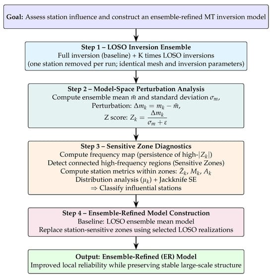
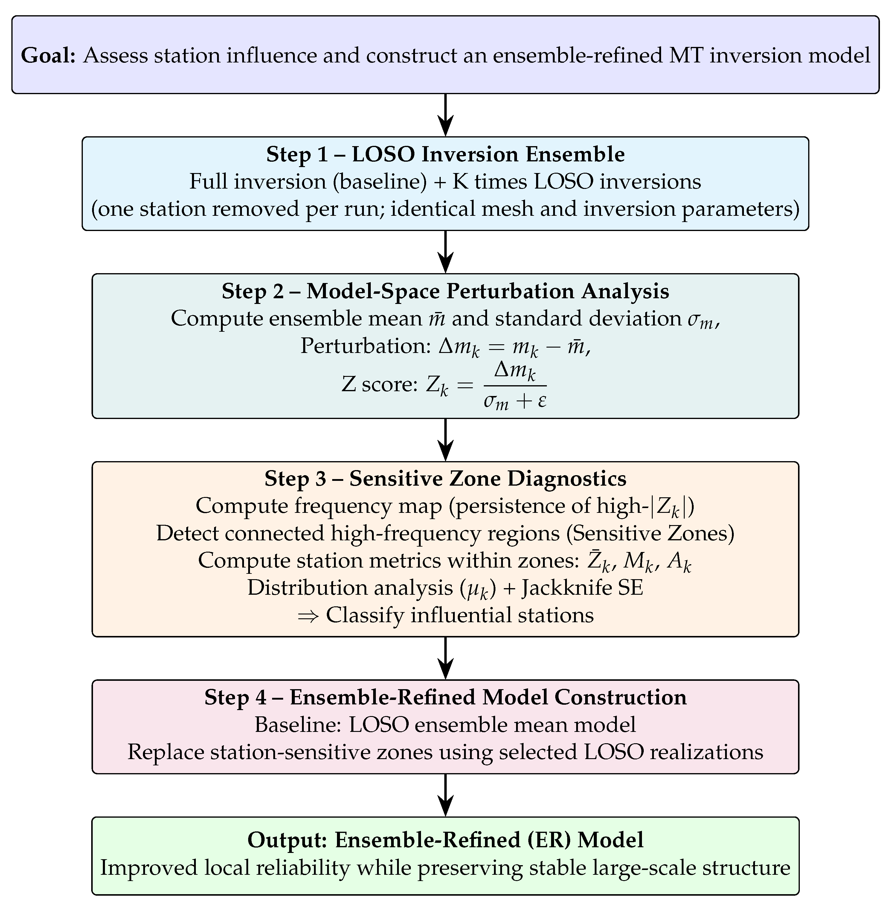
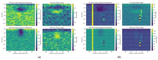
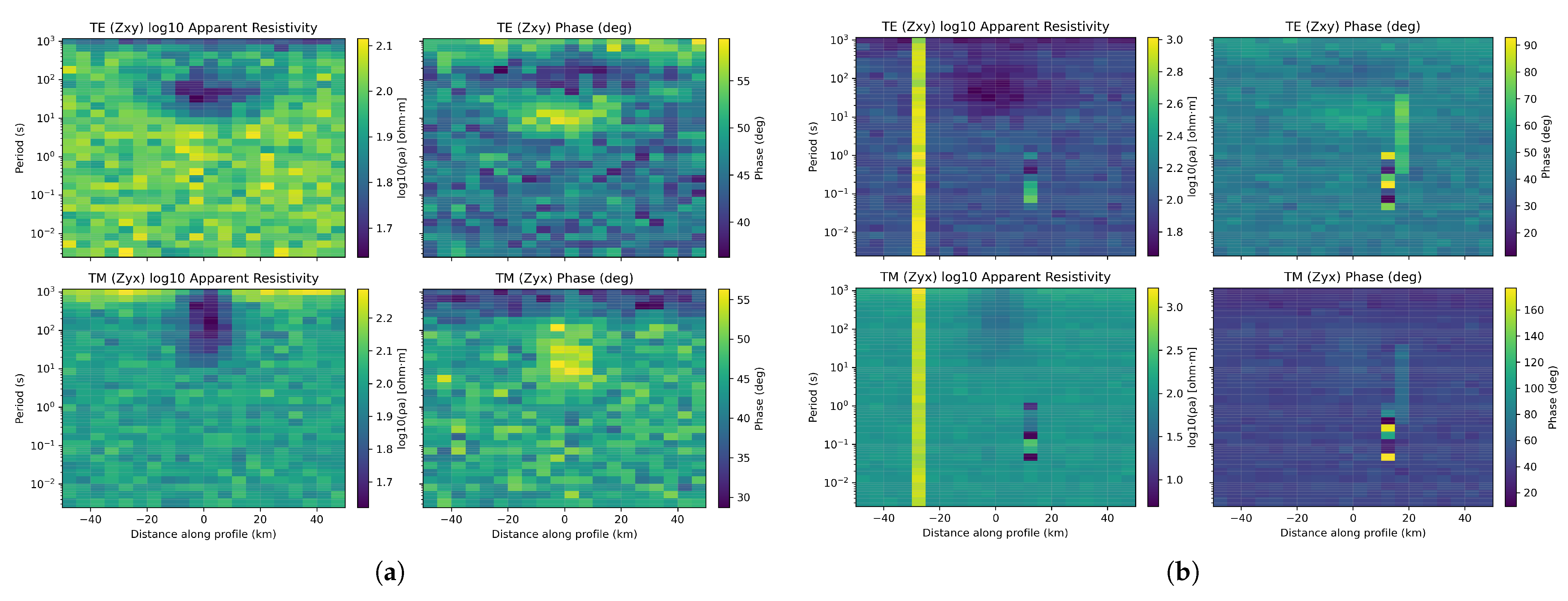
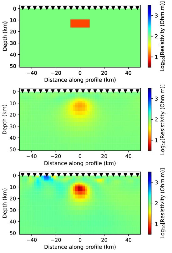
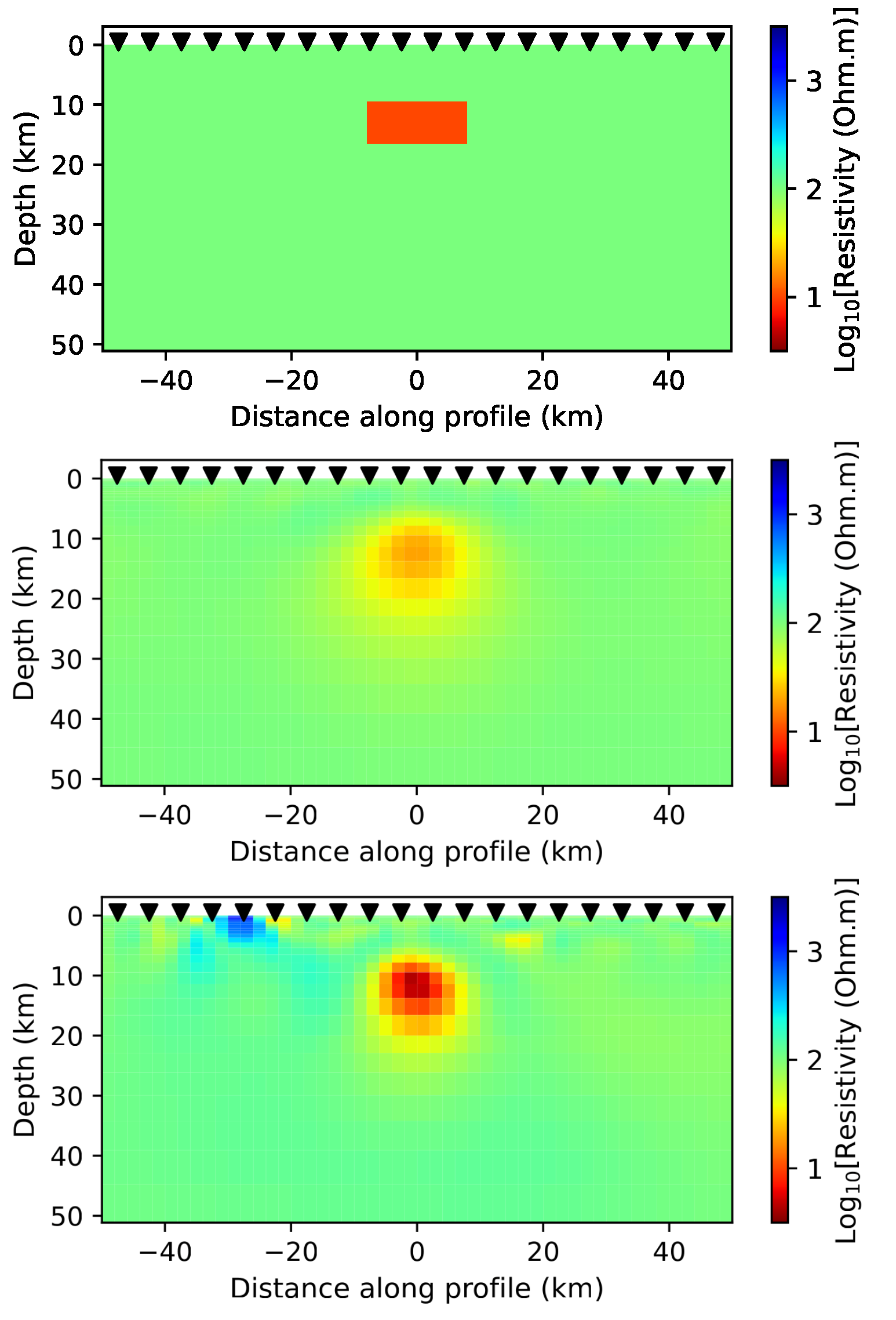
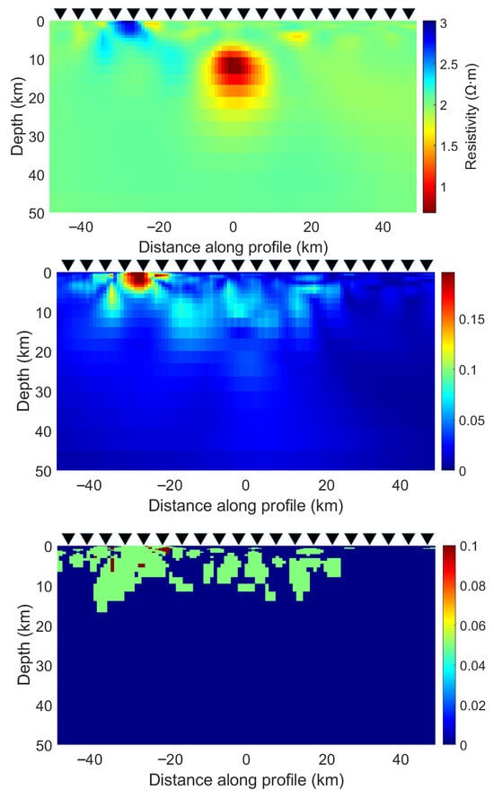
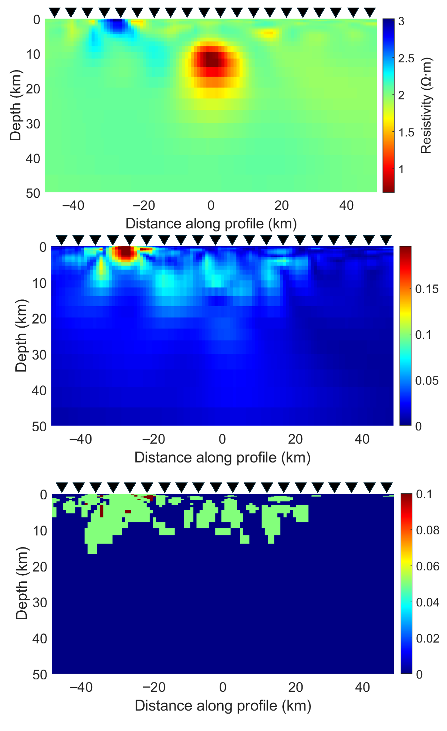
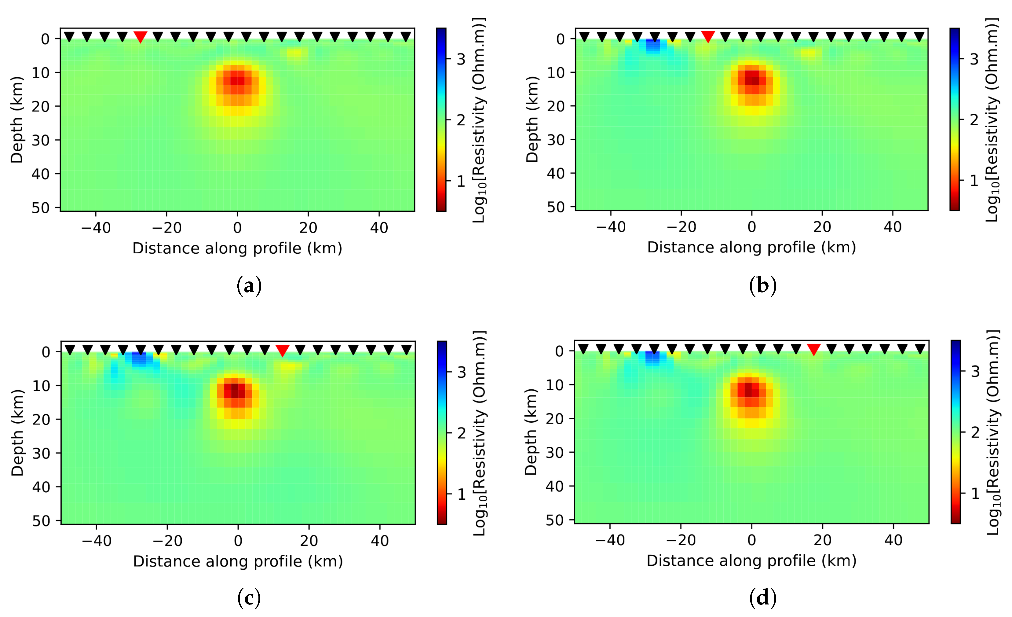
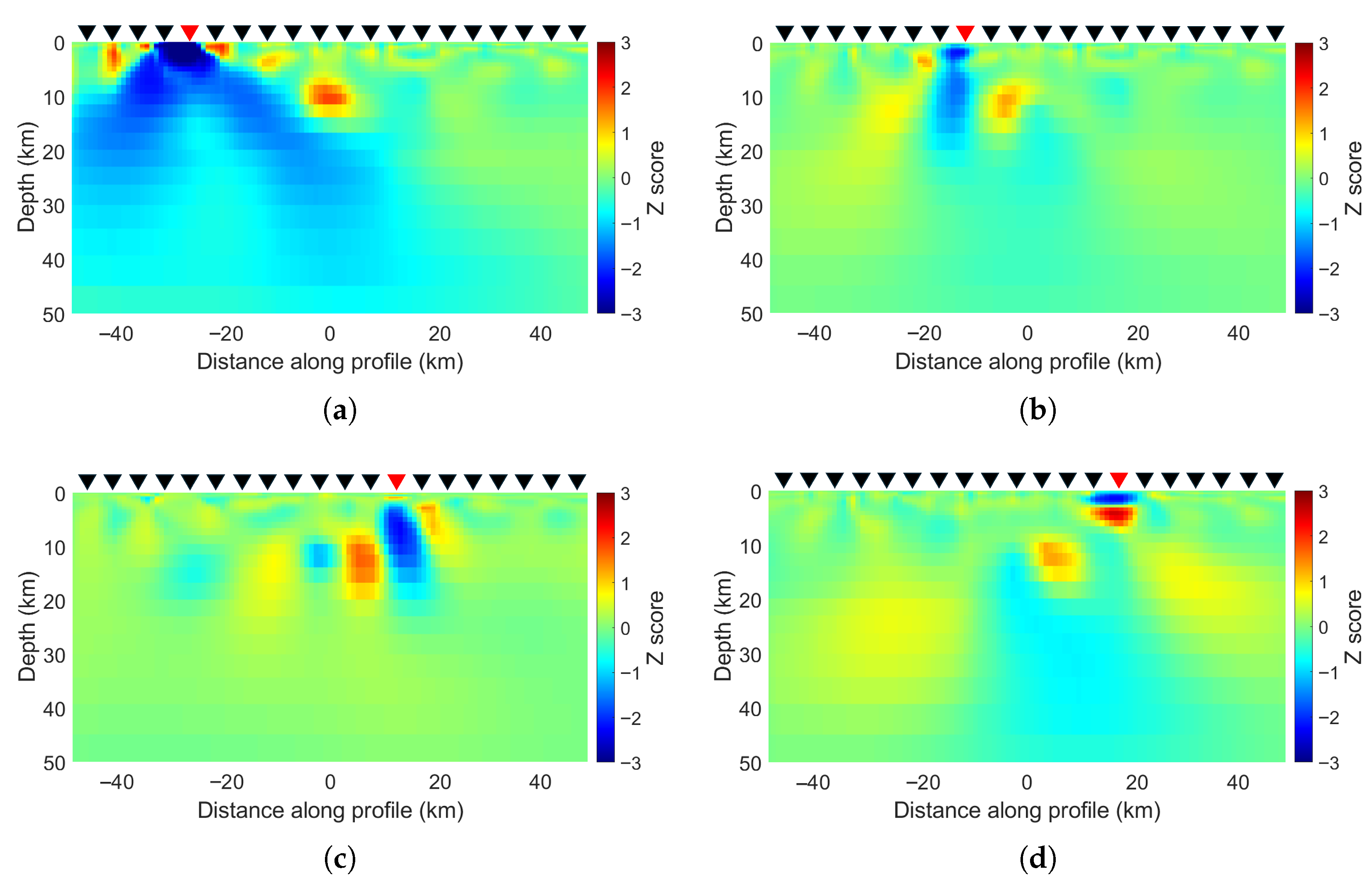
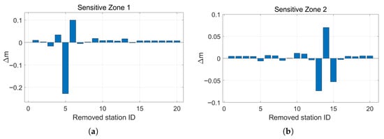
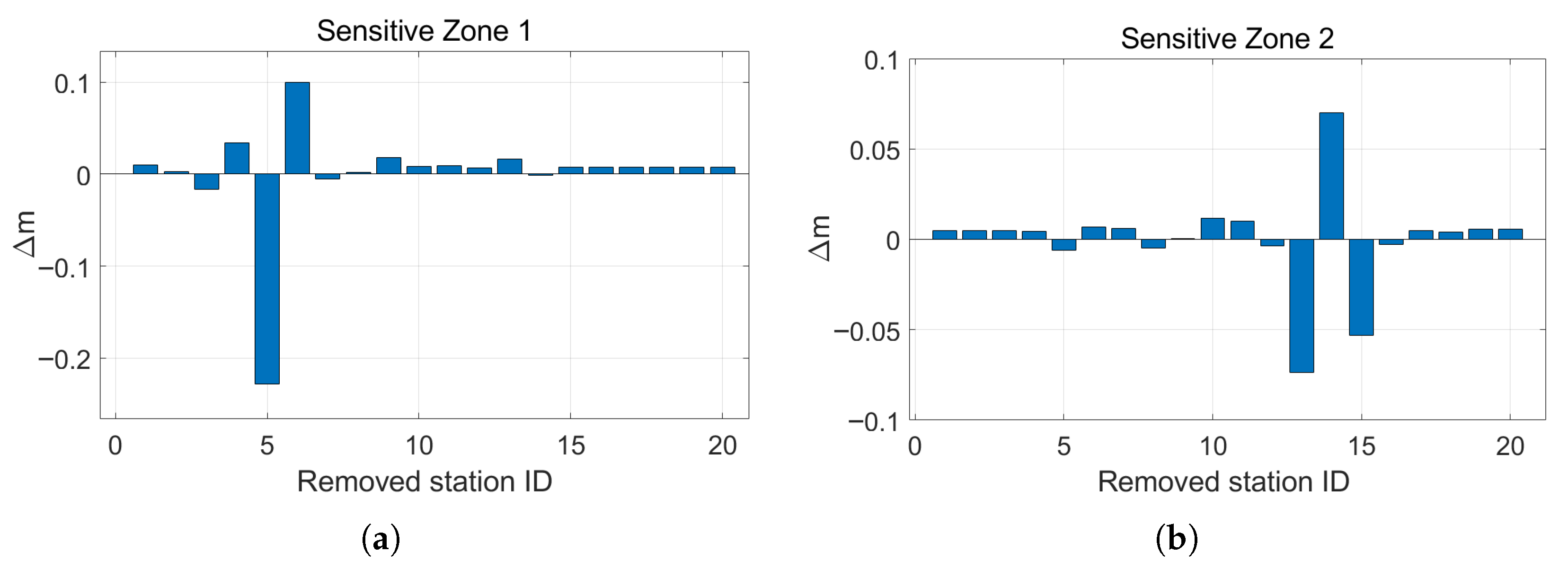
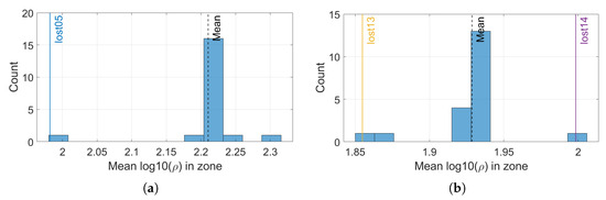
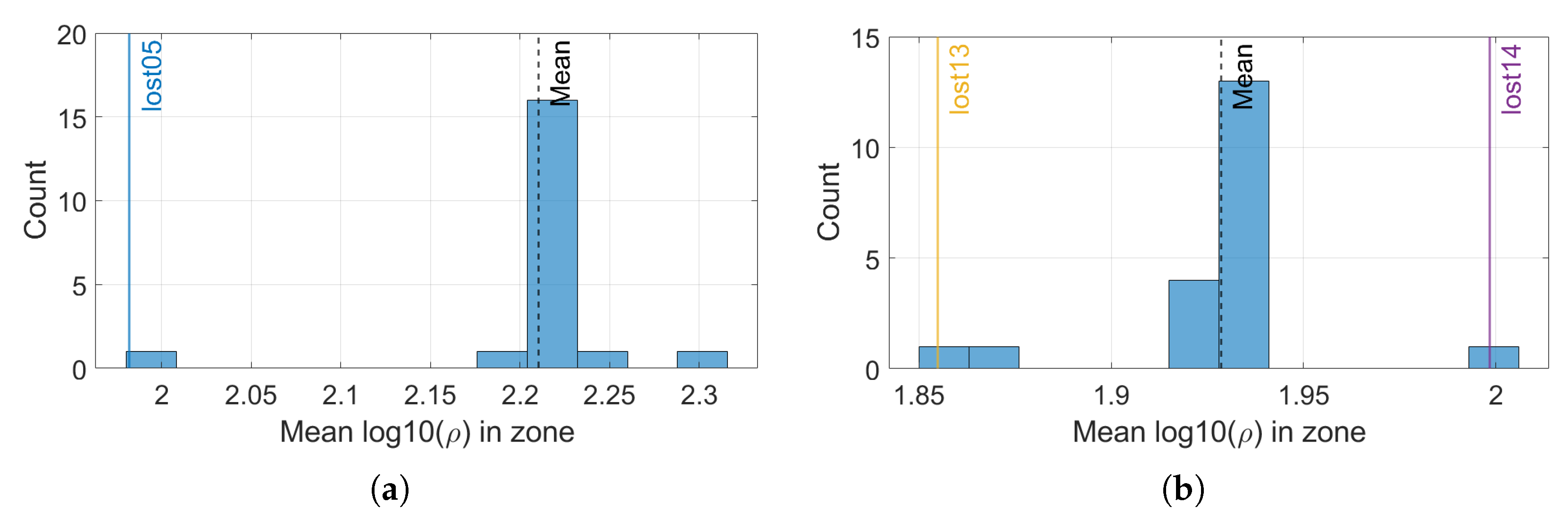
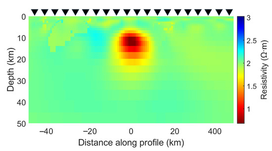
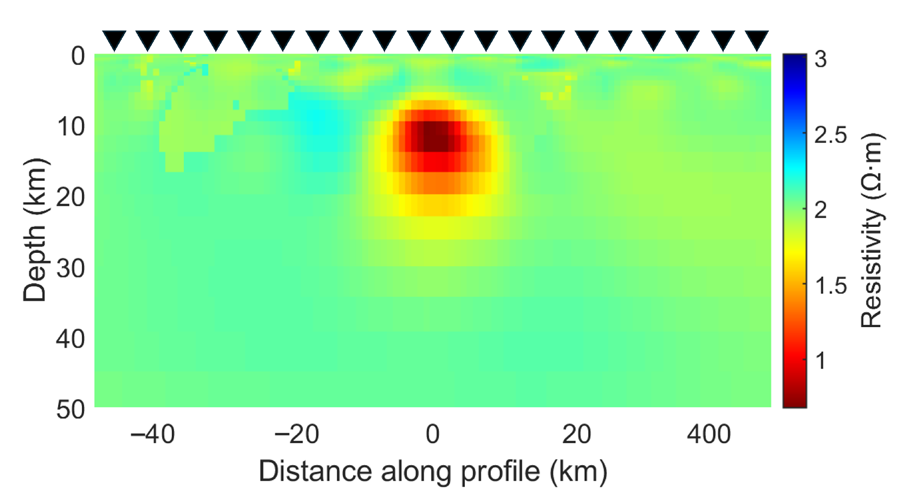
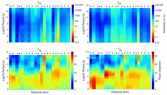
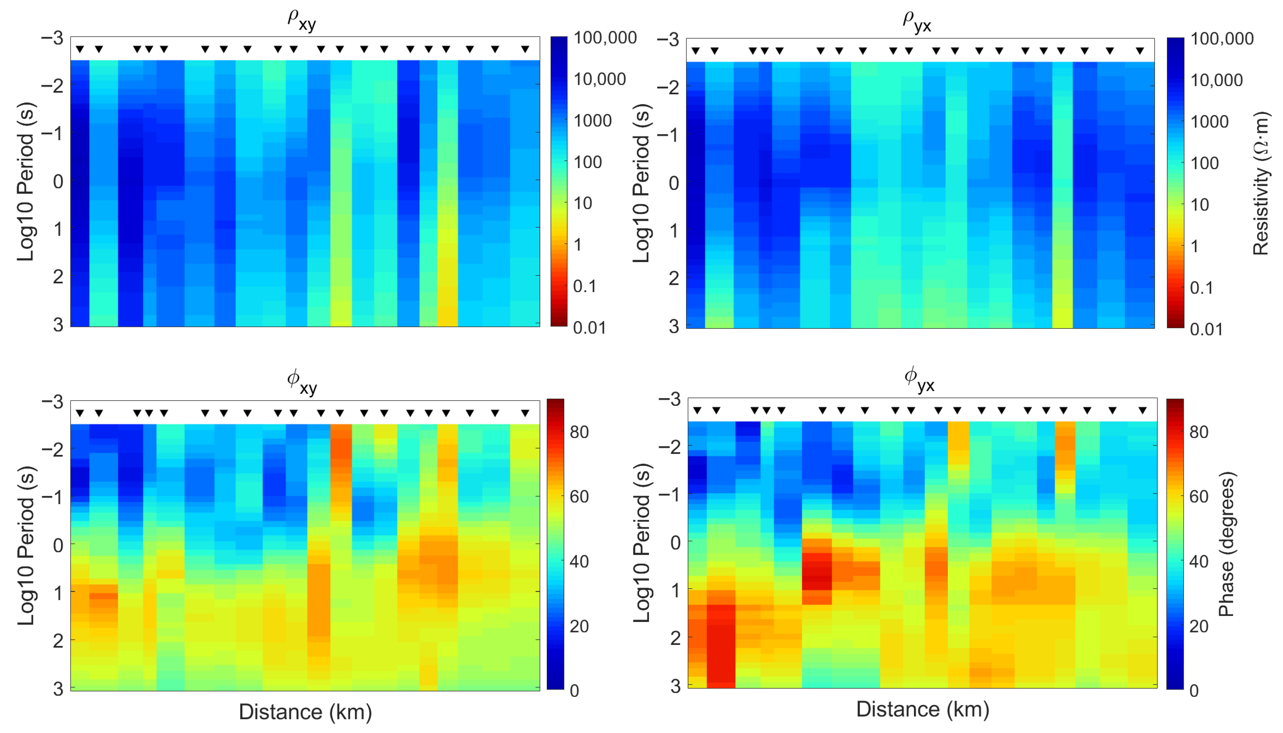
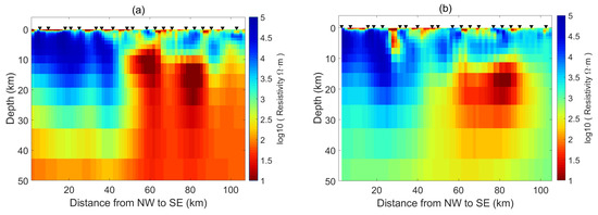
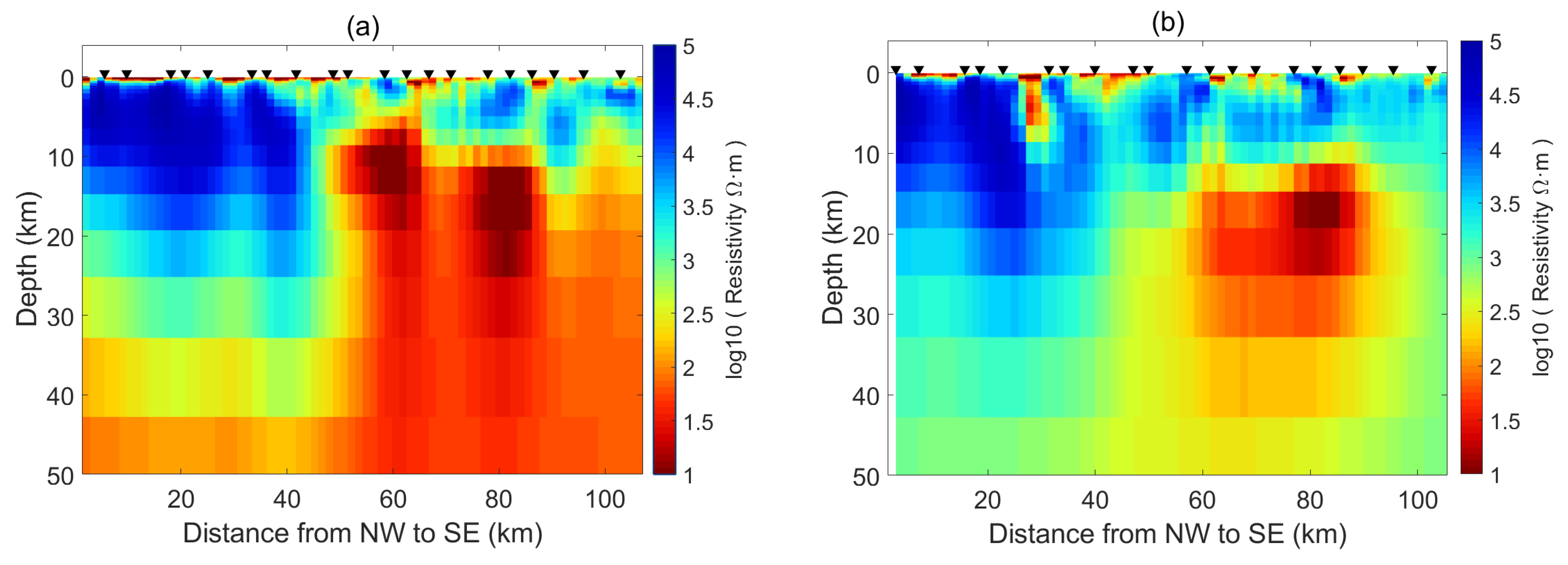
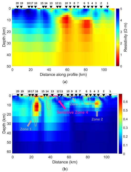
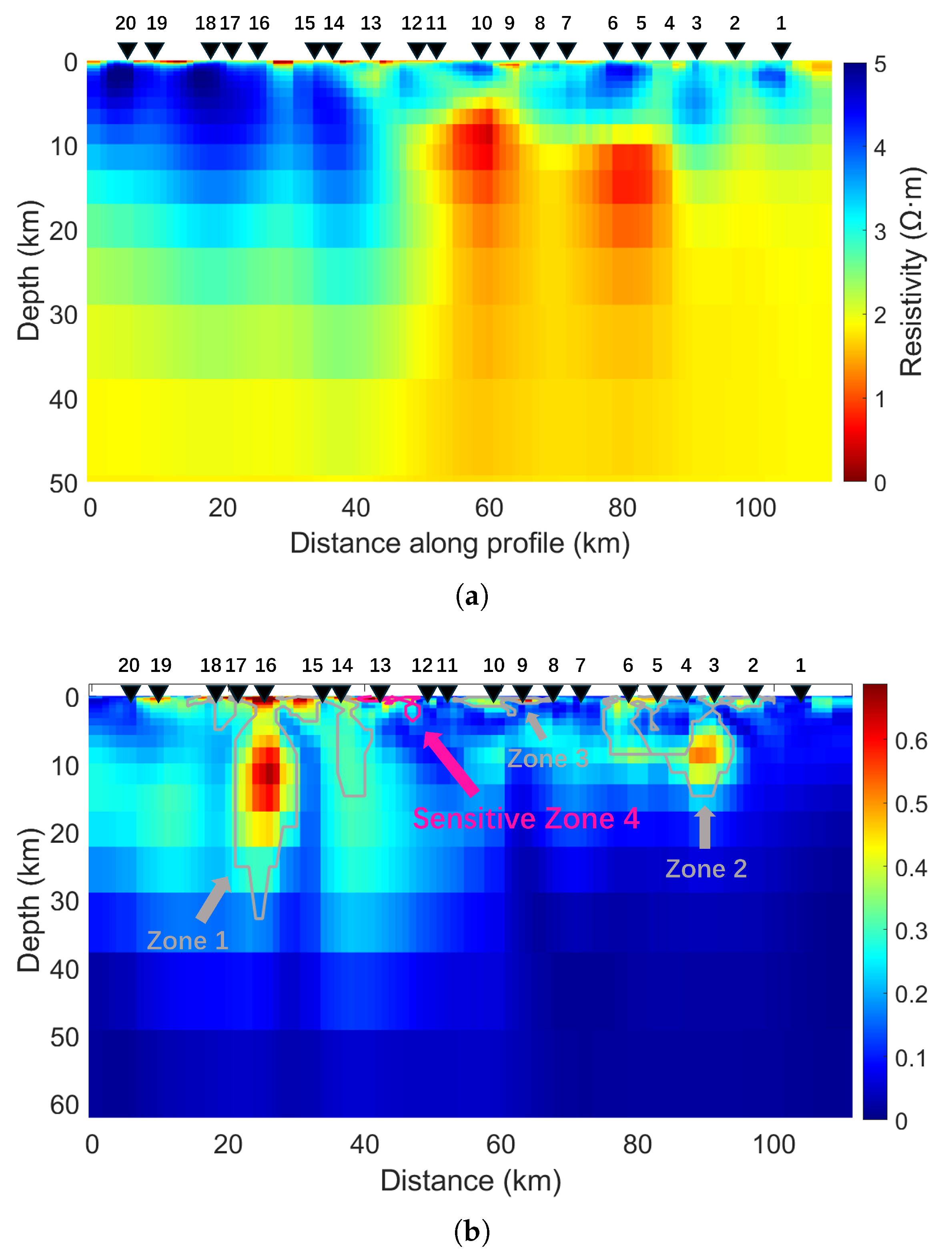
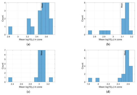
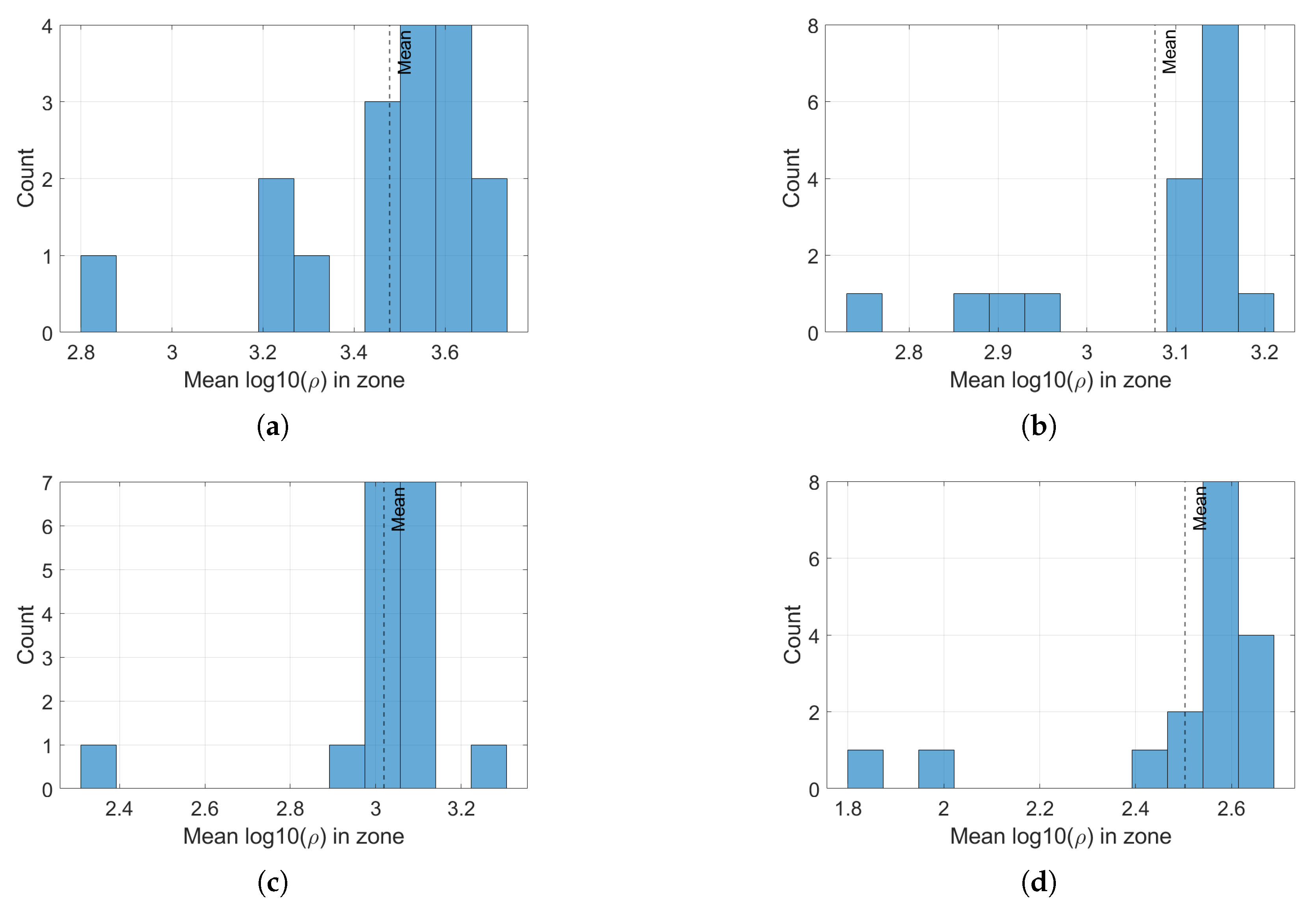
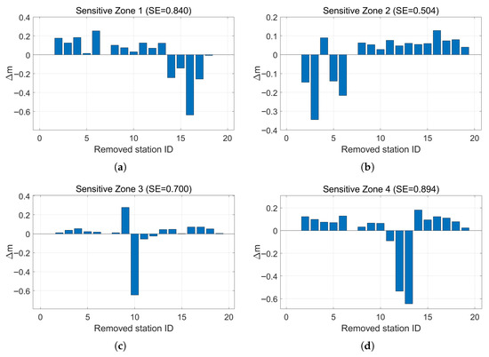
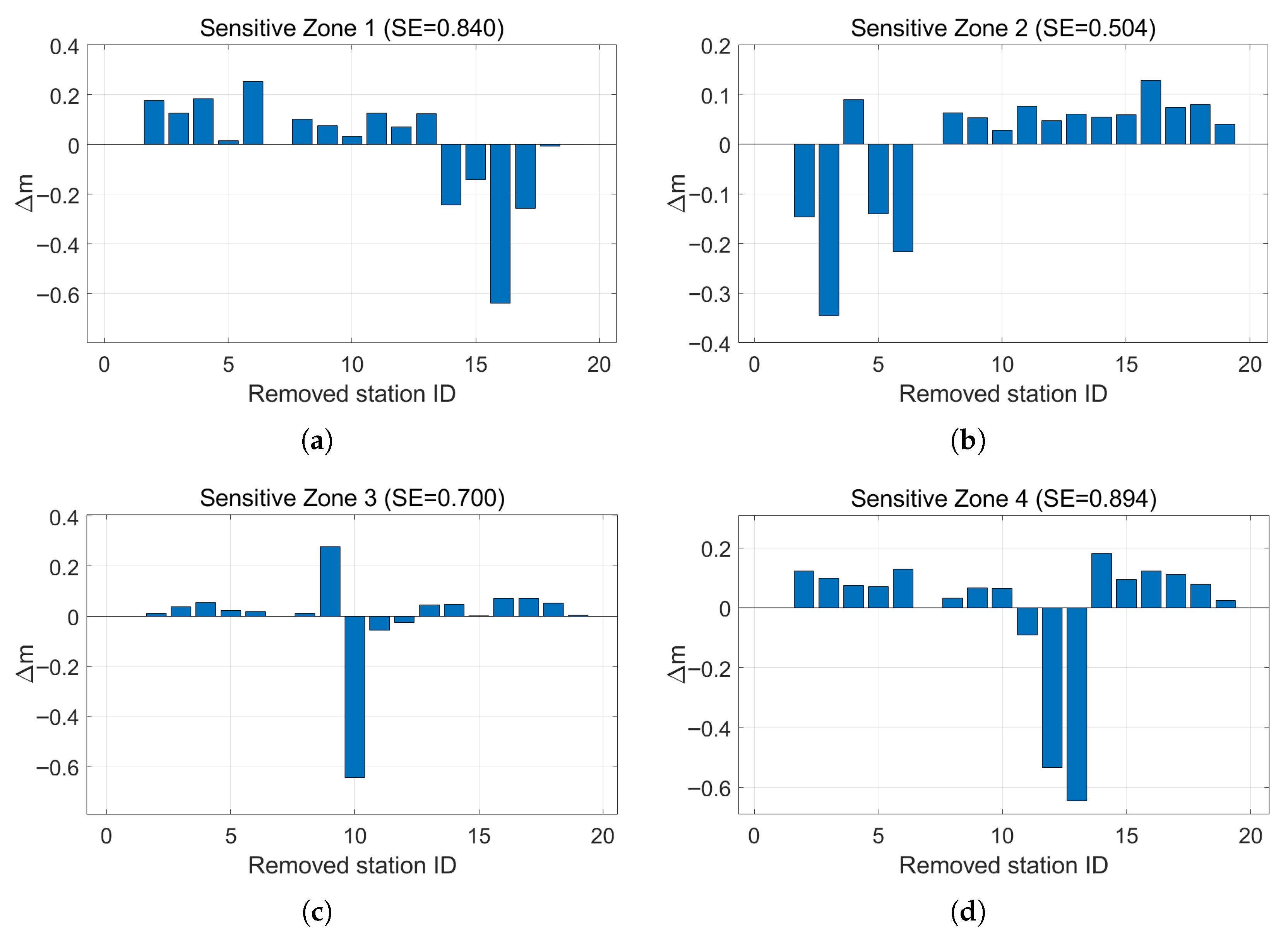
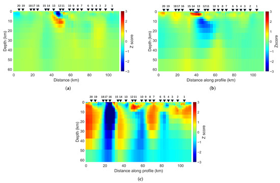
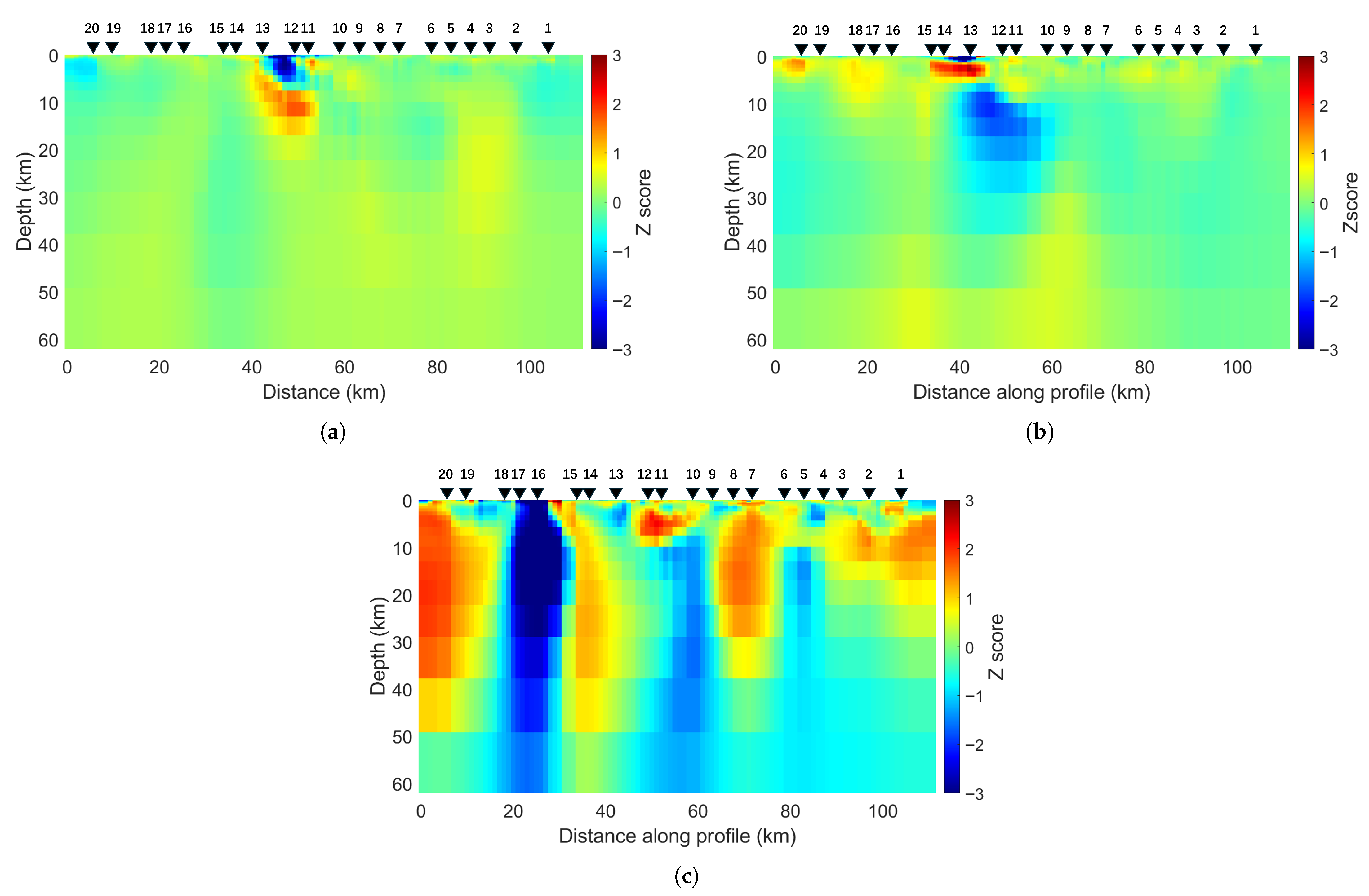
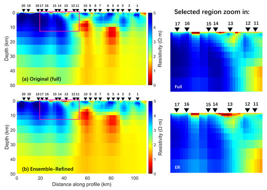
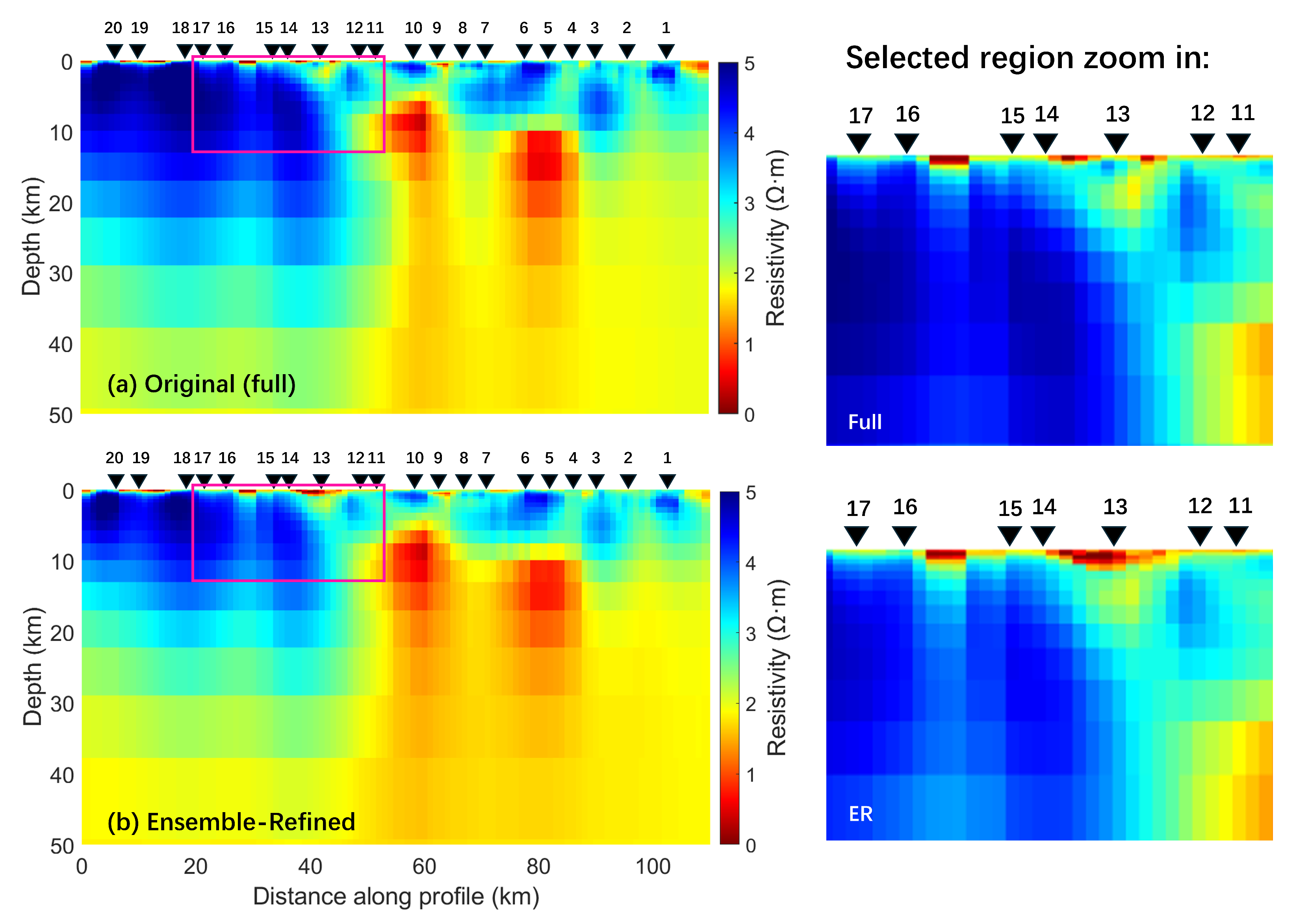
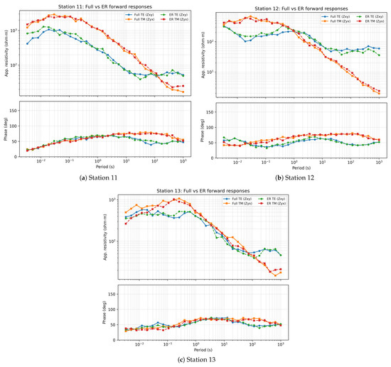
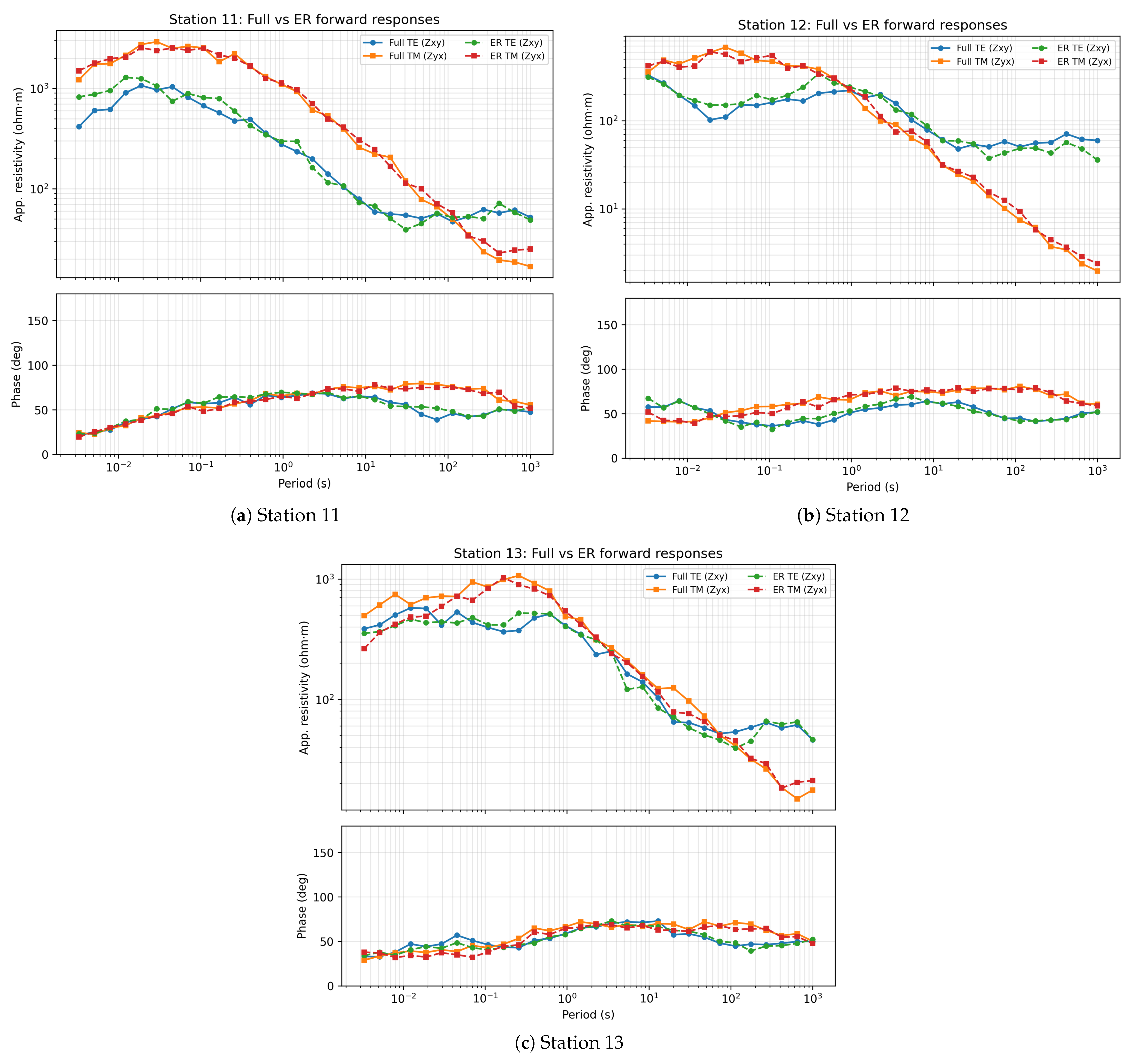

Disclaimer/Publisher’s Note: The statements, opinions and data contained in all publications are solely those of the individual author(s) and contributor(s) and not of MDPI and/or the editor(s). MDPI and/or the editor(s) disclaim responsibility for any injury to people or property resulting from any ideas, methods, instructions or products referred to in the content. |
© 2026 by the authors. Licensee MDPI, Basel, Switzerland. This article is an open access article distributed under the terms and conditions of the Creative Commons Attribution (CC BY) license.