


Abstract
Soil erosion assessments for policy are often derived from continental-scale datasets, but their suitability for regional planning remains unclear. This study compares two Revised Universal Soil Loss Equation (RUSLE) applications for Tuscany, Italy: one using high-resolution regional data (TuscReg) and another using European-scale data from the European Soil Data Centre (TuscNat). We found the mean estimated actual soil erosion rate was 58% higher in the regional assessment (10.7 vs. 6.8 Mg ha−1 yr−1). Remarkably, the spatial patterns diverged significantly in the complex landscapes characterizing some Tuscan soil regions. In mountainous areas like the Apuan Alps, TuscReg estimated soil erosion control (potential minus actual erosion) to be over 500 Mg ha−1 yr−1 greater than TuscNat for 30% of the area. Correlation analysis revealed these major differences were primarily driven by disparities in the rainfall erosivity (R) and soil erodibility (K) factors. Our results demonstrate that while EU-scale models provide a consistent, broad-scale overview, they can substantially underestimate erosion and the ecosystem service of erosion control in specific, high-risk environments. To implement policies like the EU Soil Monitoring Law (Directive (EU) 2025/2360), regional-scale data are essential to accurately identify priority areas for soil conservation and set meaningful local thresholds.
1. Introduction
Soil is a multifunctional system supporting critical ecosystem services from biomass production to carbon storage and water regulation, which are undermined by various threats [1,2]. In 2006, the European Union (EU) established a European Thematic Strategy for Soil Protection [3], renewed in the EU Soil Strategy for 2030 [4], which identifies seven major soil threats: compaction, erosion, salinization, organic matter decline, landslides, pollution, and sealing [5]. Among these, soil erosion by water is a primary driver of land degradation, leading to soil truncation, fertility loss, and diminished ecosystem services, with often irreversible impacts on a finite soil resource [6,7,8,9].
Accurate mapping of soil erosion across scales, from continental to local, is essential for informing policies such as the Common Agricultural Policy (CAP), the UN Sustainable Development Goals (SDGs), and the UN Convention to Combat Desertification (UNCCD) [10]. Moreover, soil erosion risk maps guide conservation planning, help target agri-environmental measures, and support commitments like Land Degradation Neutrality (SDG 15.3). The recent EU Soil Monitoring and Resilience Law [11] further stresses the need for standardized reference approaches and harmonized, yet regionally adaptable, methods and data, allowing soil-related thresholds to reflect Europe’s diverse pedoclimatic conditions rather than imposing a uniform approach.
The Revised Universal Soil Loss Equation (RUSLE) [12] is a widely adopted empirical model for estimating long-term average soil loss from sheet and rill erosion valued for its flexibility, data accessibility, and comparability across regions [10]. It provides a scientifically justifiable indicator of erosion rate (Mg ha−1 yr−1) [12]. However, the reliability of this indicator depends heavily on the scale and quality of input data, which determine how well local environmental, terrain and soil conditions are represented [13]. Since the RUSLE model is designed to estimate soil loss from sheet and rill erosion, it does not account for other erosive processes such as landsliding or gullying, which, therefore, are not considered in this study.
Many European countries, including Italy, lack harmonized national soil erosion databases at the detailed scales required by decision makers (regional, provincial, and local). Consequently, national-scale assessments often rely on continental-scale datasets, such as those from the European Soil Data Centre (ESDAC) [14,15,16]. These may differ significantly from regional-scale applications that use local data at higher resolution, such as those available for Veneto [17], Emilia-Romagna [18], and Marche [19]. Understanding the comparability and discrepancies between EU-scale and regional-scale erosion products is, therefore, crucial to assess their respective suitability to support regional policies and land planning.
This study focuses on Tuscany (central Italy), which possesses a detailed regional soil database and for which a RUSLE-based erosion mapping was conducted within the framework of EJP SOIL [20] internal project SERENA [21]. We compare two RUSLE applications: one using high-resolution regional data (TuscReg) and another using ESDAC data (TuscNat). Despite the availability of both data types, a systematic, quantitative analysis of their differences in estimating erosion and erosion control—a key ecosystem service indicator—is lacking. We hypothesize that discrepancies will be greatest in areas of complex topography and high climatic variability, primarily due to differences in the rainfall erosivity (R) and soil erodibility (K) factors. Therefore, the objectives of this study are: (i) to quantitatively and spatially compare soil erosion and erosion control maps from TuscReg and TuscNat across Tuscany and its soil regions; (ii) to identify which RUSLE factors drive the main differences; and (iii) to discuss the implications for soil conservation policy and land use planning. These comparisons are vital for evaluating soil health and ensuring that erosion management strategies are based on appropriately scaled information.
2. Materials and Methods
2.1. Study Area
Tuscany covers ≈ 23,000 km2 (9–12° E, 42–44° N) and exhibits remarkable variability in landscapes, climate, and land use. The climate ranges from Mediterranean along the coast (Figure 1) to temperate inland. Average annual temperatures range from 10–13 °C along the Apennine ridge to 15–17 °C along the coast. Mean annual precipitation varies from about 400 mm in the southernmost areas and exceeds 2000 mm in the Apuan Alps. Land use patterns are closely linked to topography: plains are largely occupied by urban settlements and agriculture, whereas hills and mountains are a mosaic of farmland, grassland, and forest. Forests cover nearly half of Tuscany’s territory [22].
Tuscan landforms include coastal plains and marine terraces along the coast in the west, extensive river valleys, and hilly to mountainous terrain extending toward the Apennine range, reaching elevations up to 2054 m a.s.l. Notable geomorphological features include the Apuan Alps (1946 m a.s.l.), Monte Amiata (1485 m a.s.l.), the rolling Chianti Hills (892 m a.s.l.), the Mugello Valley, and the Colline Metallifere (1060 m a.s.l.). The region’s complex morphology and geology create a wide range of pedo-landscapes with distinct soil properties and dynamic geomorphic processes [22].
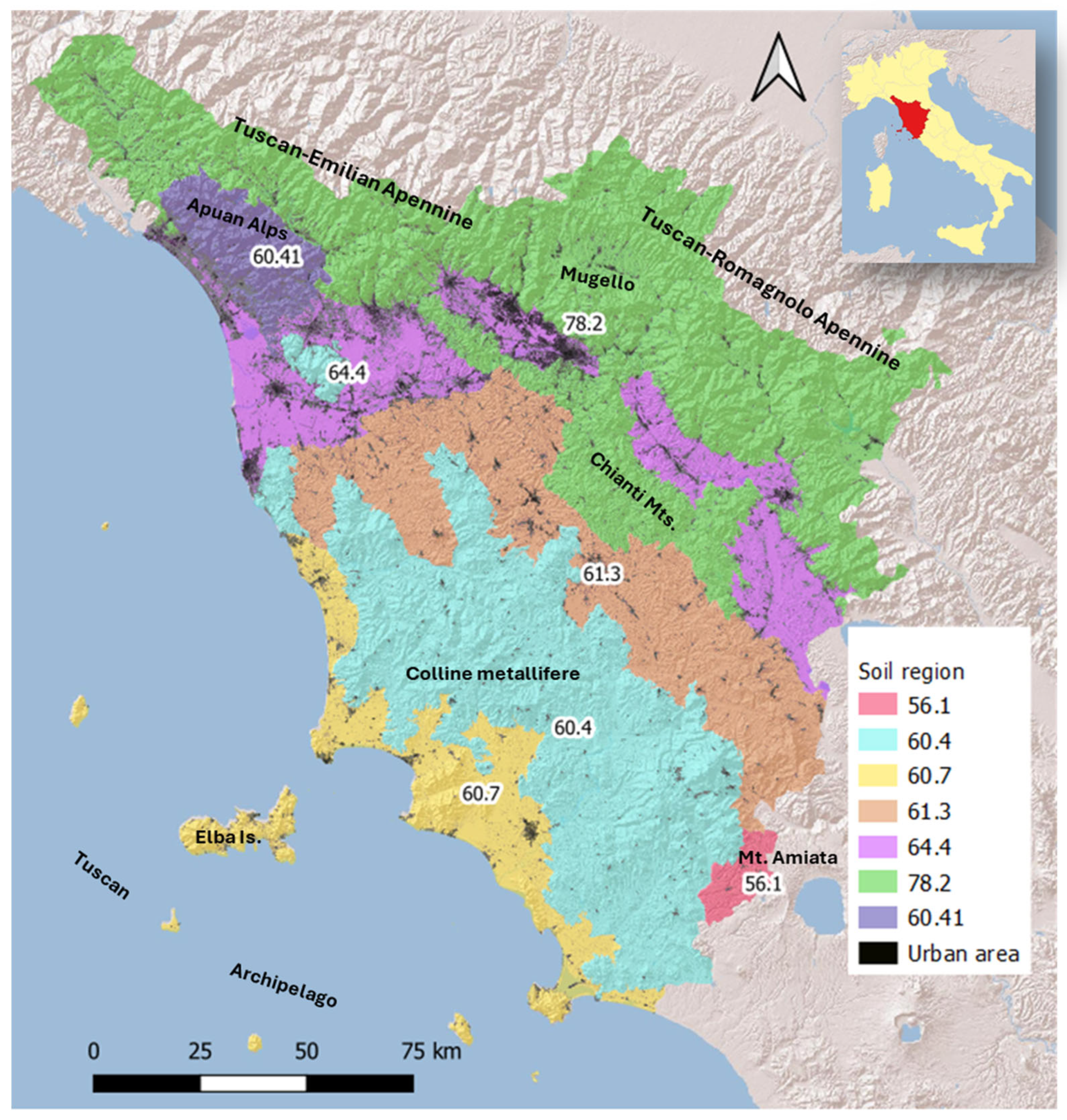
According to the World Reference Base (WRB) for Soil Resources [23], Cambisols are the most common type in hilly areas, while Vertisols and Luvisols typically occur in alluvial plains and older geological formations, particularly along the southern coast. Regosols and Leptosols are widespread along the Chianti uplands and the Apennine ridges, where Podzols also occur locally under coniferous forests. Andosols are restricted to the remnants of the Quaternary volcanic district in southern areas. Tuscany comprises seven soil regions—areas with soils sharing similar climatic, lithological, and morphological conditions (Figure 1) [24,25,26].
Figure 1.
Soil regions of Tuscany [25]: 78.2: mountainous ranges of the central and northern Apennines; 60.41: mountainous ranges of northwest Tuscany (Apuan Alps); 64.4: alluvial inland plains and coastal plains of northern Tuscany; 60.4: hilly and mountainous ranges of central Tuscany; 61.3: hills of central Tuscany on Pliocene and Pleistocene deposits; 60.7: coastal plains, including hills and archipelago islands; 56.1: hills of southern Tuscany on extrusive volcanic rocks (Mount Amiata). Map delineated at a reference scale of 1:1,000,000 based on climatic and geological differences.
2.2. Methodological Approach and Available Data
The Revised Universal Soil Loss Equation (RUSLE) [12,27] estimates the mean annual soil loss rates by sheet and rill erosion (other forms of water erosion, such as gully erosion, are not estimated by the model). The RUSLE does not assess deposition either. The model has the following form:
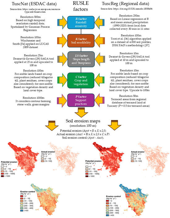
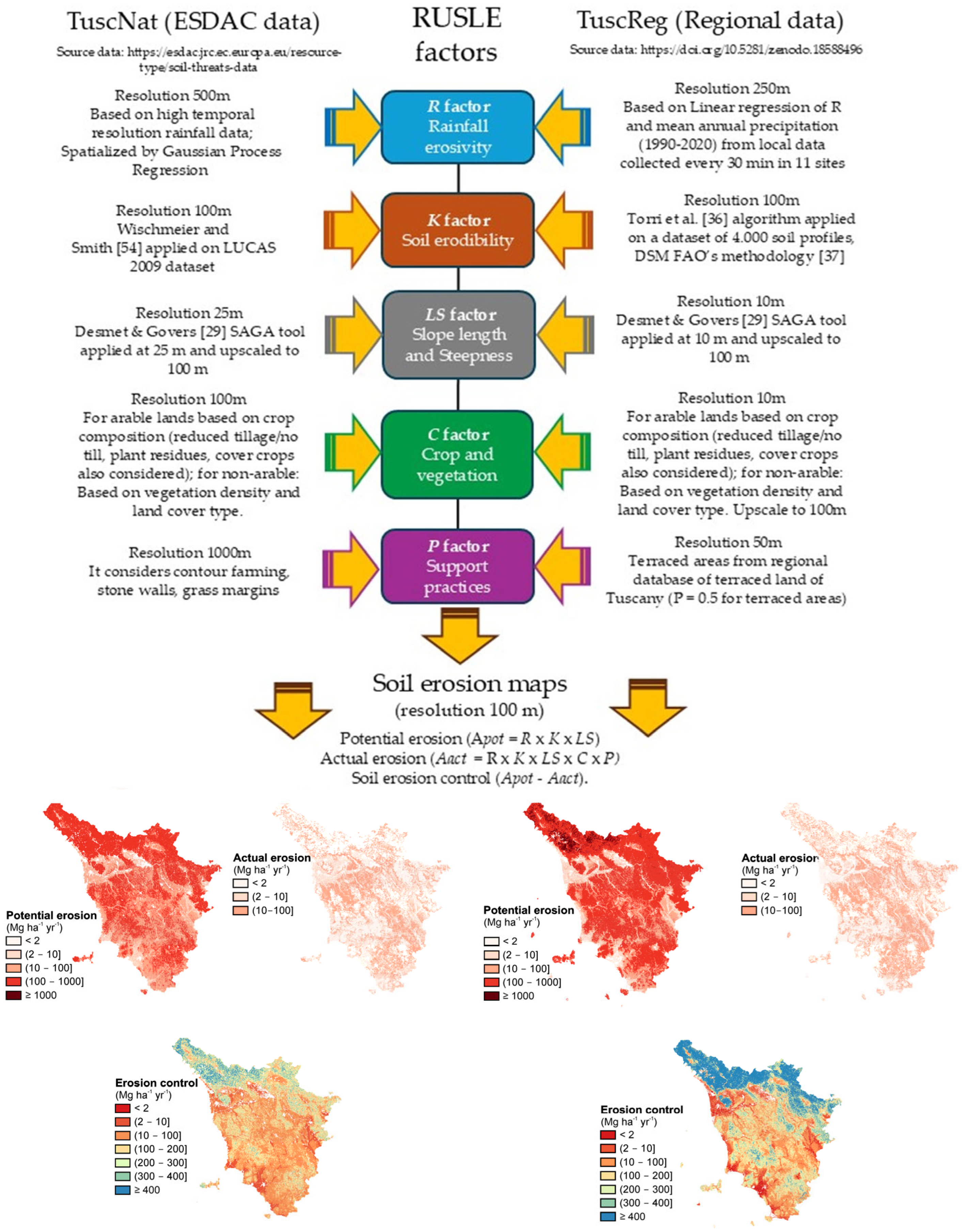
where A (Mg ha−1 yr−1) is the annual average soil loss, R (MJ mm ha−1 h−1 yr−1) is the rainfall-runoff erosivity factor, K (Mg ha h ha−1 MJ−1 mm−1) is the soil erodibility factor, LS (dimensionless) is the slope length and slope steepness factor, C (dimensionless, ranges between 0 and 1) is the cover-management factor, and P (dimensionless, ranges between 0 and 1) is the support practices factor. Figure 2 shows the entire methodological workflow for both the TuscNat and TuscReg assessments. The workflow reports the data sources and summarizes the processing steps and the resolution for each RUSLE factor and the final erosion estimates.
A = R × K × LS × C × P
Figure 2.
Entire methodological workflow for both the TuscNat and TuscReg assessments.
2.2.1. RUSLE Factor Assessment Based on ESDAC Datasets
All data for the application labeled “national” were requested from ESDAC in March 2024. All the layers were provided as raster files in ETRS89-extended/LAEA Europe EPSG: 3035. They were reprojected to EPSG:3003 (Monte Mario/Italy zone 1) through bilinear resampling to a 100 m resolution for comparisons with the regional-based application. Below, we describe each RUSLE factor for the national application.
- Rainfall-runoff erosivity factor (R factor)
The R factor for the national application is based on Panagos et al. [28]. It was downloaded from https://esdac.jrc.ec.europa.eu/content/rainfall-erosivity-european-union-and-switzerland (accessed on 20 February 2026). They estimated R from the rainfall data of several regional and national bodies in the EU to determine the kinetic energy of 30 min rainfall events (although for many stations, 1 h rainfall data were used and made compatible through regressions). The data were then spatialized using Gaussian process-based regression (with monthly climate, terrain, and geographic covariates). In their estimation, Italy was one of the countries with the highest number of weather stations (251) with rainfall data but with a relatively limited temporal coverage of around 10 yrs on average [7]. The original map is available at 500 m resolution, and thus, it was downscaled to 100 m.
- Soil erodibility factor (K factor)
The K factor for the national assessment is based on Panagos et al. [16] and was downloaded from https://esdac.jrc.ec.europa.eu/content/soil-erodibility-k-factor-high-resolution-dataset-europe (accessed on 20 February 2026). The K factor was estimated by combining data from the LUCAS 2009 sampling campaign for soil organic matter and texture of topsoils (0–30 cm). Structural and permeability classes were assigned according to existing pedotransfer functions or main textural groups, and the resulting K factor was corrected for the surface stone fraction. The K factor was spatially interpolated, combining regression (cubist models based on geographical and environmental covariates) with the splines of the residuals of the regression models. The data was available at 100 m resolution.
- Slope length and slope steepness factor (LS factor)
The national LS is based on a 25 m resolution digital elevation model (DEM), derived from a hybrid ASTER/SRTM product, applying the Desmet and Govers [29] algorithm, as incorporated in SAGA ver. 9.5.0 [30], as described by Panagos et al. [31]. It was downloaded from https://esdac.jrc.ec.europa.eu/content/ls-factor-slope-length-and-steepness-factor-eu (accessed on 20 February 2026) and upscaled to 100 m to be used at the same resolution as the other layers.
- Cover-management factor (C factor)
The C factor was derived from the work by Panagos et al. [32] and downloaded from https://esdac.jrc.ec.europa.eu/content/cover-management-factor-c-factor-eu (accessed on 20 February 2026). They estimated C using CORINE land cover data from 2014, differentiating between arable and non-arable land. For arable land, they estimated C values for different crops based on the literature and assigned a C value to a location based on the proportion of crops present in the location (derived from statistical data in Eurostat) and the C values obtained in their literature review. They furthermore weighed cropland C values in terms of the management practices of tillage, cover crops, and the use of crop residues based on information on the proportion of arable land under a particular management practice. For non-arable lands, the C factor value of a location determination was based on the values found in the literature and weights that consider the fraction of land cover under a particular land cover class. The C factor layer was available at 100 m resolution.
- Support practices factor (P factor)
The P factor for the national application was based on Panagos et al. [33] and downloaded from https://esdac.jrc.ec.europa.eu/content/support-practices-factor-p-factor-eu (accessed on 20 February 2026). They based the estimation of P on a combination of weights for different slope values derived from a high-resolution DEM (25 m) for the contour P subfactor. Additionally, they used LUCAS 2012 records for the soil conservation practices of stone walls and grass margins to derive P subfactor values for these conditions, derived from the literature. They used ordinary kriging to interpolate the stone walls and grass margins of the LUCAS sampling points to the extent of the whole EU and then combined the contour, stone walls and grass margins’ subfactors into a single P factor value. As the original layer was available at 1000 m resolution, it was downscaled to 100 m.
2.2.2. RUSLE Factor Application Based on Regional Databases
In the following sections, each factor of the RUSLE used for the regional application in Tuscany is described according to the information provided by regional services. All the layers were originally in EPSG:3003. All layers were scaled to 100 m (using bilinear interpolation) in order to make them comparable with those of the national application.
- Rainfall-runoff erosivity factor (R factor)
The R factor was calculated from interpolated data of mean annual rainfall for the period 1990–2020, a product elaborated by the meteorological database available at the Lamma Consortium (https://www.lamma.toscana.it/en, accessed on 20 on February 2026) algorithm [34], which interpolates meteorological values using a digital elevation model (DEM). The original algorithm was calibrated for Tuscany; the input data is a dataset collected from 1995 to 2017 in 965 thermometric stations and 1403 pluviometric stations. The calculation of the R factor for the calibration was done using a linear regression between the R factor and mean annual precipitation (R2 = 0.94), obtained from 30 min precipitation data for 11 stations in Mugello (FI) [35]. The original layer is available at 250 m resolution.
- Soil erodibility factor (K factor)
The K factor for the regional application was obtained through the algorithm proposed by Torri et al. [36], which uses, as inputs, soil textural size fractions (sand, silt, and clay; USDA limits) and organic matter concentration. The above input data were obtained from the regional soil database (https://www502.regione.toscana.it/geoscopio/pedologia.html, accessed on 20 February 2026), which was then interpolated over a 100 m resolution grid covering Tuscany [37].
- Slope length and slope steepness factor (LS factor)
The LS factor for the regional application followed the same methodology as that for the national one but was elaborated from a DEM with a 10 m resolution (https://www502.regione.toscana.it/geoscopio/cartoteca.html).
- Cover-management factor (C factor)
A similar methodology to that described for the national application was used to derive the C factor for the regional application. For arable lands, the same values from the literature and the same coefficients for residue management, cover crops and no tillage were used, while for non-arable lands, the fraction cover was calculated from Copernicus Sentinel images. In this case, the values of the C factor were calculated based on the fraction cover, resorting to Google Earth Engine, taking 2018 as the reference year [32]. The vector of the regional land use and the landcover database were used (https://www502.regione.toscana.it/geoscopio/usocoperturasuolo.html, accessed on 20 February 2026) to derive C at 10 m resolution.
- Support practices factor (P factor)
The P factor was determined using the regional database of “terraced areas”, a non-freely available layer created by the Lamma Consortium (https://www.lamma.toscana.it/). It represents areas where terraces and embankments, which were created in the past, are widely spread. The terraced areas were assigned a P factor value of 0.5 based on expert judgement. The original layer is available at 50 m resolution.
2.2.3. RUSLE Implementation
Soil loss was estimated at a common 100 m resolution using the raster data layers of each RUSLE factor for the two different applications. In the rest of the article, these are referred to as TuscReg (our estimation) and TuscNat (ESDAC estimation) applications. The administrative boundary of Tuscany was used to delineate the area of interest for the following estimations: (i) potential erosion (Apot = R × K × LS), (ii) actual erosion (Aact; see Equation (1)), and (iii) soil erosion control (Apot − Aact). We then analyzed the results of both applications using specific ranges of erosion values (value classes) for the different erosion estimations. The classes were defined for ease of comparisons, yet some represent soil erosion thresholds set in environmental policy (e.g., 2 Mg ha−1 yr−1 maximum in the EU Soil Monitoring Law to consider a soil “healthy” or 10 Mg ha−1 yr−1 considered the limit of “severe” erosion by the EU soil dashboard). When Aact was calculated, differences in the final total area of both TuscReg and TuscNat occurred. This indicated discrepancies in the extent of spatial gaps produced by both assessments, stemming mainly from different sources of land cover data. Due to the very small magnitude of the differences (i.e., ≈ 0.6% for TuscReg and ≈ 4% for TuscNat Aact), we considered the methodology we adopted as not being influenced by them. It should be noted that a direct validation of the model outputs against measured soil erosion data was not feasible, as spatially distributed and homogeneous experimental datasets covering the entire study area are currently unavailable. Therefore, the robustness of the regional assessment was evaluated through a comparative analysis with published experimental studies conducted in Tuscany, both at the field scale [38,39,40] and at the catchment scale [41,42,43]. While this approach does not constitute a formal validation, the estimated soil loss values and their spatial patterns fall within the ranges reported in these independent studies, suggesting that the model outputs are reasonable and physically consistent.
A spatially explicit analysis (at the co-occurring pixel level) was carried out, focusing on the differences between erosion control estimates between TuscNat and TuscReg (i.e., erosion control TuscNat − erosion control TuscReg, or Δerosion control). The analysis was performed by aligning TuscReg to TuscNat through resampling with the terra package in R [44]. Additionally, a local version of Geary’s C index [45] was applied to Δerosion control values with an 8 nearest spatial matrix (corresponding to first-order queen contiguity) to explore patterns of spatial autocorrelation at the location level through the rgeoda package in R environment for statistical computing and graphics [46]. Local Geary is an index of spatial dissimilarity showing how much a location differs from its local neighborhood (as defined by the spatial matrix definition) in terms of the variable of interest (Δerosion control in this case).
Pearson’s correlations were used to investigate the correlation between erosion rate differences between applications (differences between TuscNat and TuscReg), and the underlying RUSLE factors’ differences between assessments to determine which factors accounted for the main differences in erosion estimates between both applications.
The analysis and interpretation of the results were carried out at the Tuscany region general level and at the SR level.
3. Results
3.1. Differences in RUSLE Factors Between the National and Regional Assessments
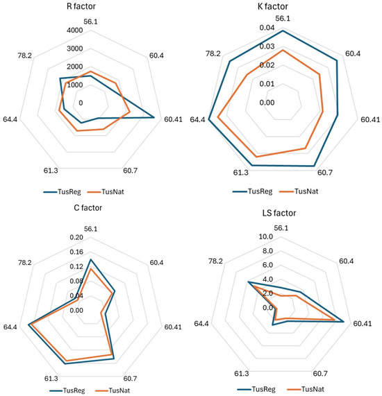
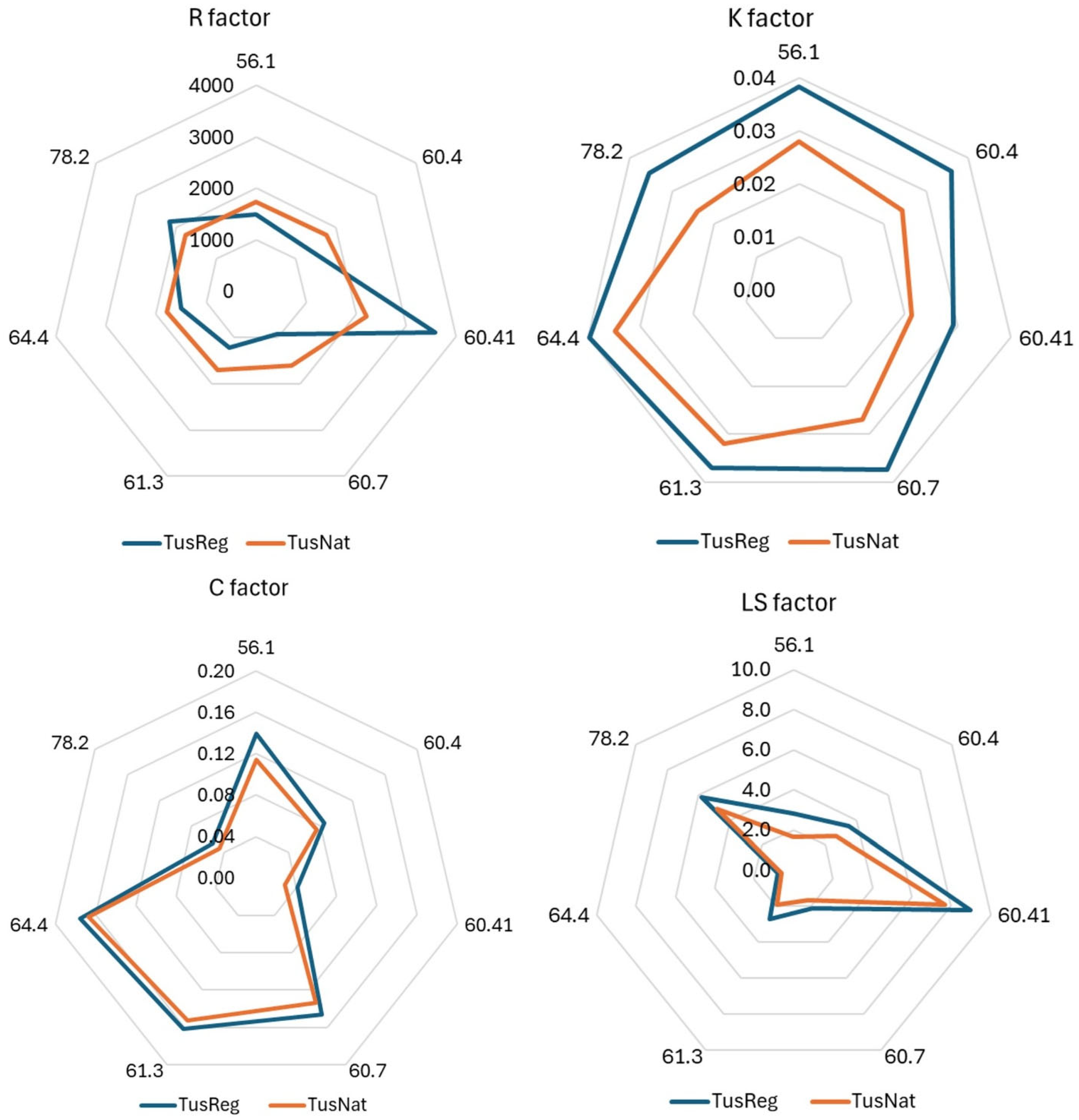
A comparison of the main statistics of the RUSLE factors for the region between the TuscNat (National Scale Application for Tuscany) and TuscReg (Regional Scale Application for Tuscany) assessments is reported in Table 1. The P factor was not included in the table, as, due to the large differences in its estimation methods, we considered the comparison inconsequential. Figure 3 graphically summarizes the averaged values at the landscape level per SR (soil region).
Table 1.
Descriptive statistics of the R (MJ mm ha−1 h−1 yr−1), K (Mg ha h ha−1 MJ−1 mm−1), LS (−), and C (-) RUSLE factors derived for the regional (TuscReg) and national (TuscNat) assessments, using the regional and ESDAC databases respectively.
Figure 3.
Mean values (zonal statistics) at soil regions (SR) level, for the TuscNat and the TuscReg assessments of the rainfall erosivity R factor (MJ mm ha−1 h−1 yr−1), the soil erodibility K factor (Mg ha h ha−1 MJ−1 mm−1), the cover management C factor (dimensionless), and the soil slope length and slope steepness (LS) factor (unitless). SR codes are reported in Figure 1.
When comparing the RUSLE factors between the two assessments, we always observed significant differences in the mean values of the factors at the SR level (p-value ≤ 0.05), mostly due to dataset size, although in several cases, very little difference occurred. For the R factor (rainfall erosivity), the two assessments showed markedly different ranges, with higher mean rainfall erosivity for TuscReg. Indeed, although the spatial patterns of higher and lower values were similar, the modeled R factor for TuscReg produced more extreme values (at both ends of the distribution) than TuscNat. The differences in the R factor between TuscNat and TuscReg were consistent, with significantly different values among SRs. Mountain landscapes presented TuscReg values much higher than TuscNat, in particular, SR 60.41 (corresponding to the Apuan Alps), and secondarily, SR 78.2 (with more heterogeneous landscapes), while in SR 60.7 (coastal plains), R was higher in TuscNat. For the K factor (soil erodibility), estimates produced by TuscReg were slightly higher than those observed for TuscNat, and differences were slightly more marked for the central hilly and mountainous areas of SRs 78.2 and 60.4. Although the results of the LS factor were very similar between the TuscNat and TuscReg assessments, TuscNat slightly underestimates LS with respect to TuscReg; the largest differences occurred in soil regions 60.41 and 56.1, namely the mountain landscapes of the Apuan Alps and Mt. Amiata, respectively. The TuscNat and TuscReg results also seemed very similar concerning the C factor, and mean values followed the same behavior among the SRs. TuscNat slightly underestimated C in all the SRs, and the largest differences occurred in SRs 56.1 (M. Amiata) and 60.41 (Apuan Alps), both dominated by forests. Larger discrepancies emerged in more fragmented land use contexts (see Supplementary Figures S7–S9).
A more in-depth examination of the spatial distribution and the differences between the two assessments is provided in the Supplementary Materials for each of the RUSLE factors, except for the P factor.
3.2. Actual Erosion, Potential Erosion and Soil Erosion Control Comparisons
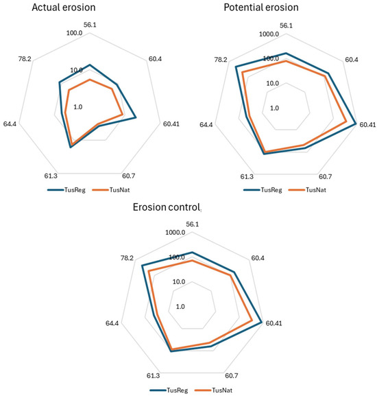
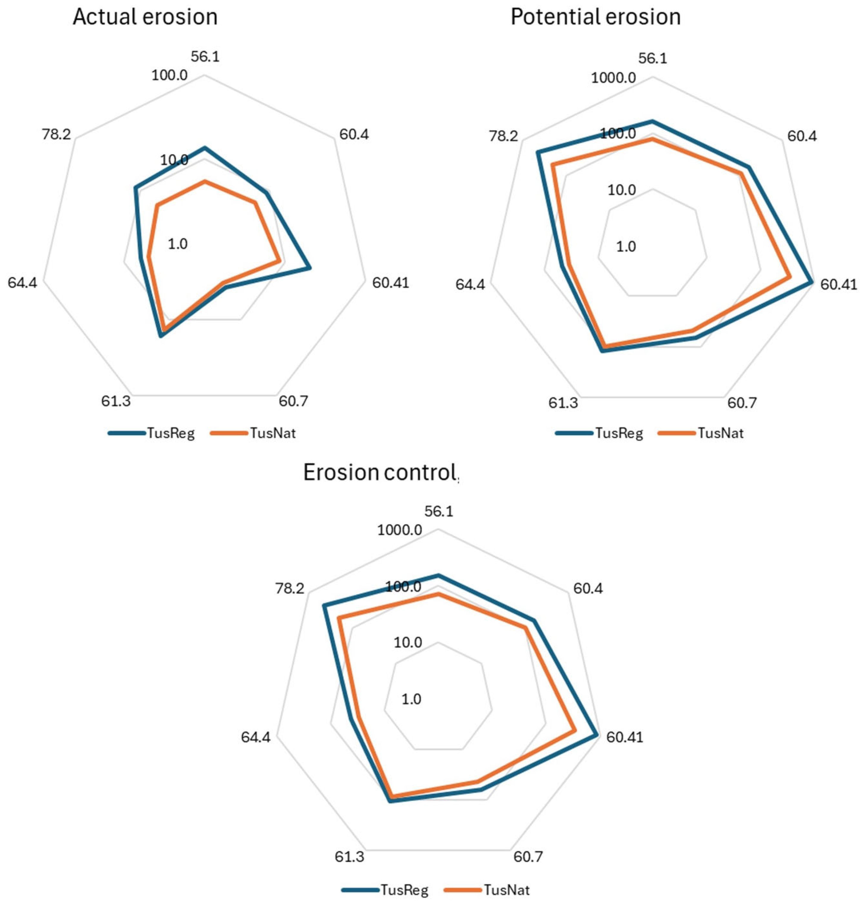
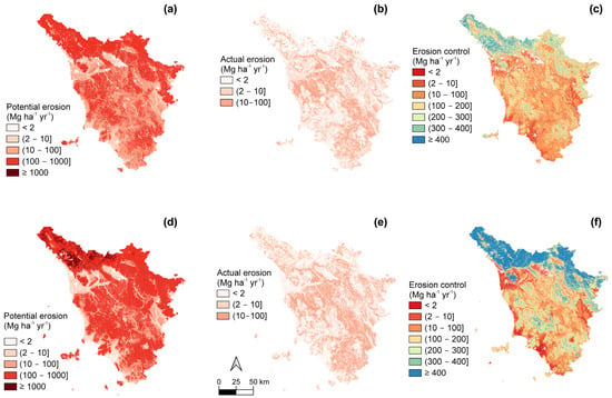
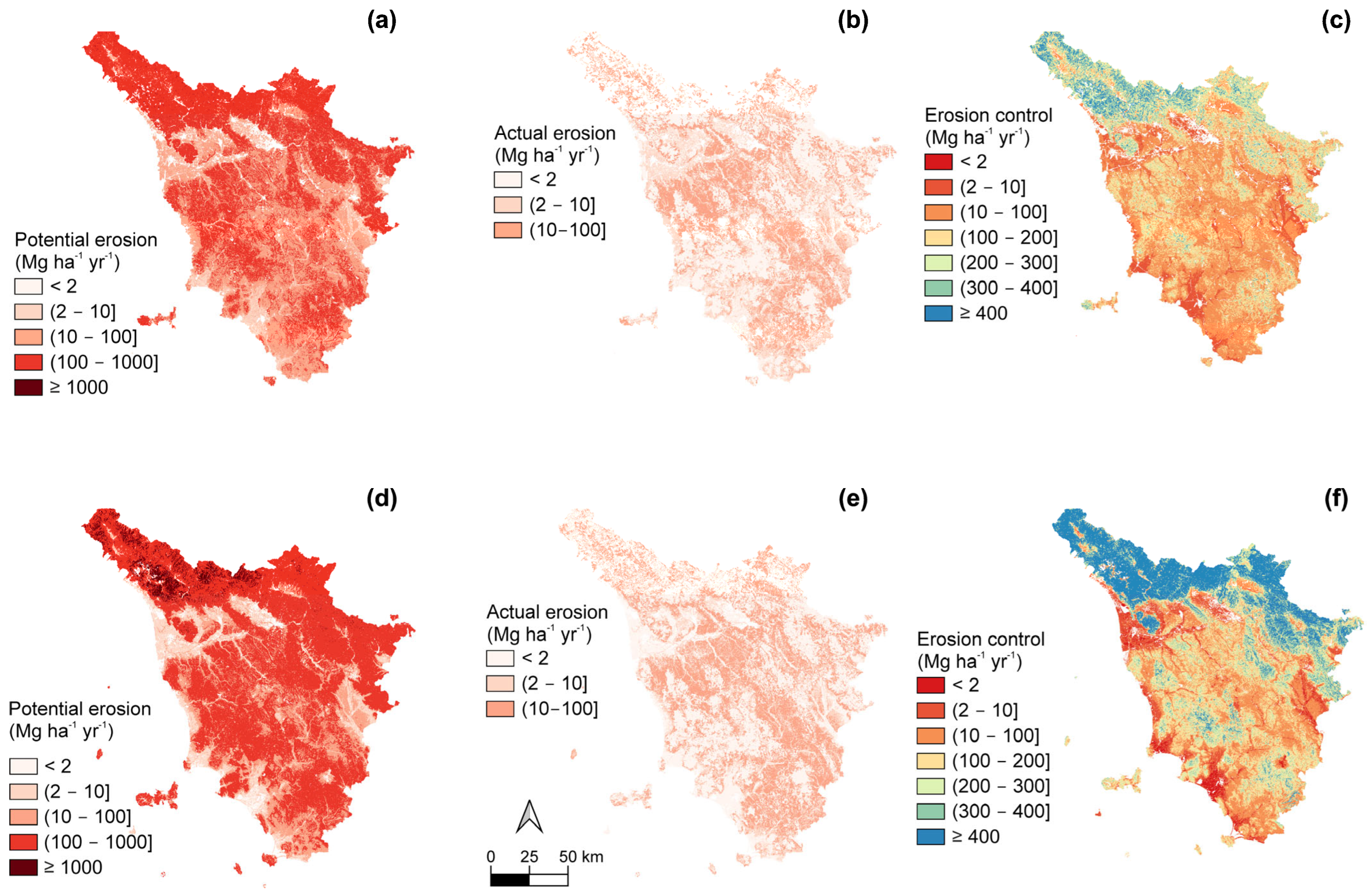
Table 2 and Figure 4 summarize the results per SR for actual erosion, potential erosion, and erosion control. In general, Apot (Potential Soil Loss) rates (Mg ha−1 yr−1) were much higher in the NW and NE parts of Tuscany, characterized by high precipitation and a complex mountain landscape (SR 78.2, including Apennines and pre-Apennine hills, and SR 60.41, with Apuan Alps) (Figure 5). Further territories with high erosion potential corresponded to areas characterized by complex landscapes, particularly those linked to SRs with hill systems (60.4), such as the Colline Metallifere in central-W, the mountain–hill system of Mount Amiata in the south, or the western part of Elba Island (Figure 5). These areas did not necessarily correspond to the highest estimates of Aact (Actual Soil Loss), as they are mostly covered by forest vegetation.
Table 2.
Summary statistics of actual and potential soil erosion rates and soil erosion control rate (Mg ha−1 yr−1) for the whole Tuscany region (based on count = 21,553,800 locations).
Figure 4.
Mean values at the SR level for the TuscNat and TuscReg assessments of soil erosion (Mg ha−1 yr−1), potential soil erosion (Mg ha−1 yr−1), and soil erosion control (Mg ha−1 yr−1) (count = 35,000 random points).
Figure 5.
Estimates of potential erosion (left panels), actual erosion (middle panels), and soil erosion control (potential–actual, (right panels)) in Tuscany, central Italy. Estimates were calculated using RUSLE with either national-level data from the European Soil Data Centre (ESDAC) (a–c) or from Tuscany regional-level data (d–f).
Percentages of land area under reference soil loss classes for Apot and Aact are reported in Table 3. Larger differences in land area between the two assessments were observed for Apot (Table 3), where TuscReg produced a larger area of low and moderate Apot classes (<2 Mg ha−1 yr−1 and 2 to 10 Mg ha−1 yr−1 respectively) and a lower area of intense Apot (class 10 to 100 Mg ha−1 yr−1) yet a larger area of heavy erosion (class 100 to 1000 Mg ha−1 yr−1) with respect to that produced by TuscNat (Table 3).
Table 3.
Percentage of land area in the region of Tuscany, central Italy, falling under a soil loss class according to either the regional (TuscReg) or the EU-ESDAC (TuscNat) erosion estimates by RUSLE. Round brackets correspond to closed intervals (containing the value), whereas square brackets denote open intervals.
For Aact, TuscReg produced a larger area under intense erosion (Table 3). Aact, as estimated by both assessments, did not exceed, in general, 100 Mg ha−1 yr−1.
Such discrepancies also resulted in marked differences in erosion control (Table 4; two additional categories were introduced to enable a more detailed assessment). The major difference in erosion control was that the TuscReg assessment returned to a higher area falling under higher supply values than TuscNat overall (Table 4), with a much higher surface area in the highest supply category. These areas of high supply were located in SRs related to mountain ranges. TuscNat showed a much higher area than TuscReg in the erosion control category of 10 to 100 Mg ha−1 yr−1, distributed in several SRs associated with hills and lowland plains (e.g., 60.4, 61.3, and 64.4).
Table 4.
Percentage of land area falling in soil loss control (potential erosion minus actual erosion) classes according to either the regional (TusRceg) or EU-ESDAC (TuscNat) erosion estimates created by RUSLE. Round brackets correspond to closed intervals (containing the value), whereas square brackets denote open intervals.
3.3. Spatially Explicit Coherence Between Assessments for Soil Erosion Control
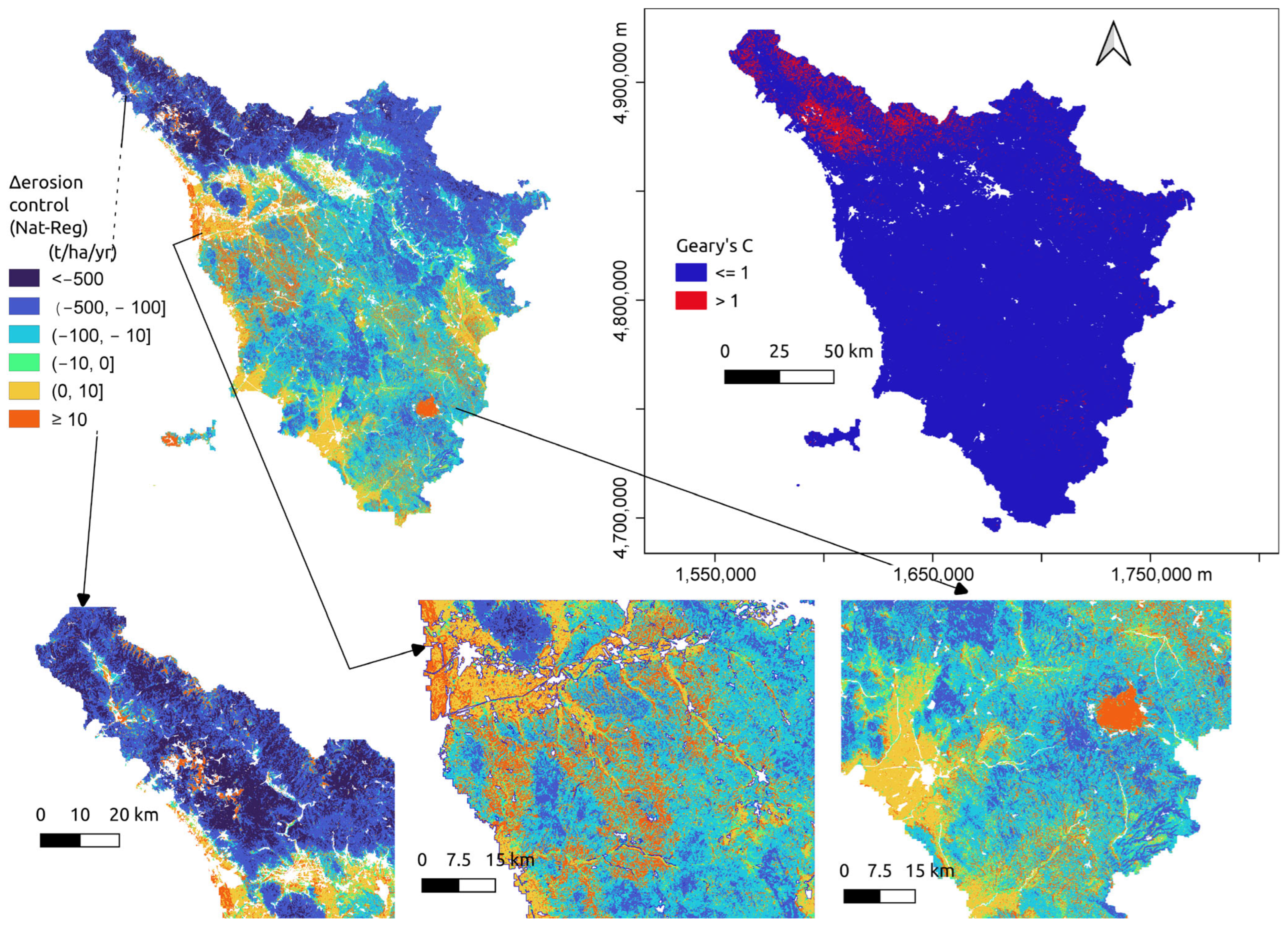
By classifying soil erosion control differences (i.e., Δerosion control at common spatial units for both assessments; see the Section 2) into several classes, some spatial patterns at the region level became evident. First, the two assessments did not yield Δerosion control in a simple linear way (i.e., an estimation consistently producing always higher or lower values; Figure 5 and Figure 6). Second, there were characteristic patterns in the spatial distribution of Δerosion control related to the landscape and soil region factors implicitly contained in the input data (we understood this in terms of terrain, soil, and vegetation). In this way, soil erosion control estimated through the TuscReg assessment yielded much higher supply (i.e., high Δerosion control negative values, corresponding to classes lower than –500, and from –500 to –100 Mg ha−1 yr−1) in the areas of more complex terrain (high LS), forest vegetation (low C), and high precipitation (high R) in the NW tip of the region (Figure 6 bottom left), associated with the SRs of the Apennines (78.2), and the Apuan Alps (60.4) (Figure 6). These TuscReg >> TuscNat classes of Δerosion control represented around 30% of the surface (for which locations were common to both assessments) in Tuscany. Additionally, the NW tip of the region was associated with negative spatial autocorrelation (i.e., higher dissimilarity) between the two assessments, as shown by the local Geary’s index (Figure 6 upper right), unlike the rest of the region. These locations with high spatial dissimilarity in Δerosion control values (first two classes) corresponded well with those where the differences in the R factor among the two assessments were particularly large (≥2000 MJ mm ha−1 h−1 yr−1; Figure 6 bottom left). In general, most of the region showed positive spatial similarity (local Geary’s C ≤ 1).
Figure 6.
Erosion control differences (Δerosion control; this is the value: erosion controlTuscNat − erosion controlTuscReg) in the region of Tuscany, central Italy (upper left). Figures in the bottom panels are magnifications of the Δerosion control map with areas of representative values. The (upper-right) panel is the spatial distribution of significant local Geary’s values in the region. Values of Δerosion control for the different classes are in Mg ha−1 yr−1.
The Δerosion control class from −100 to –10 Mg ha−1yr−1 covered 45 of the surface, and it occurred within SRs associated mainly with hills, lowlands, and coastal plains (60.4, 61.3, 64.4). The Δerosion control classes with the lowest differences between the two assessments (−10 to 0, and 0 to 10 Mg ha−1 yr−1; around 16% of the surface) were associated mainly with SRs located on lowland plains (64.4, and 60.7), annual croplands, and (secondarily) permanent crops (Figure 6, bottom center). Finally, the class representing zones where TuscNat yielded higher erosion control (class of 10 Mg h−1 yr−1 and higher; around 8% of the surface) occurred mainly in SR 61.3 under different land covers; on small clumped locations on mountainous SRs 60.41 and 78.2; and in a single location in SR 60.4 with complex terrain, that of Mount Amiata (Figure 6, bottom right). In mountain locations, the differences between the two assessments were mainly due to the much higher values of the K factor estimated through TuscNat (Figure 3), so the estimates of Apot from TuscNat were higher than those in TuscReg, and as such, TuscNat produced higher soil erosion control estimates. Differences in estimates of the R factor between the two assessments were the main reason for the differences between the two assessments. TuscNat estimated significantly higher R values than TuscReg in all SRs, except those with mountain landscapes, such as 78.2 (Central and Northern Appennine) and 60.41 (Apuan Alps), where R factor values were significantly higher for TuscReg.
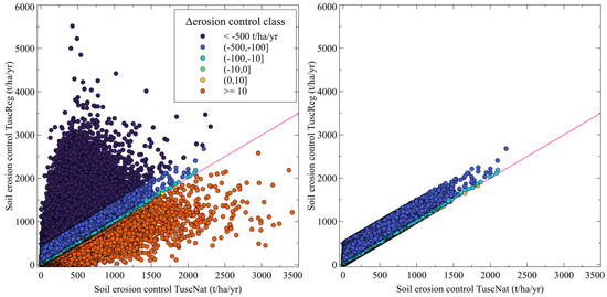
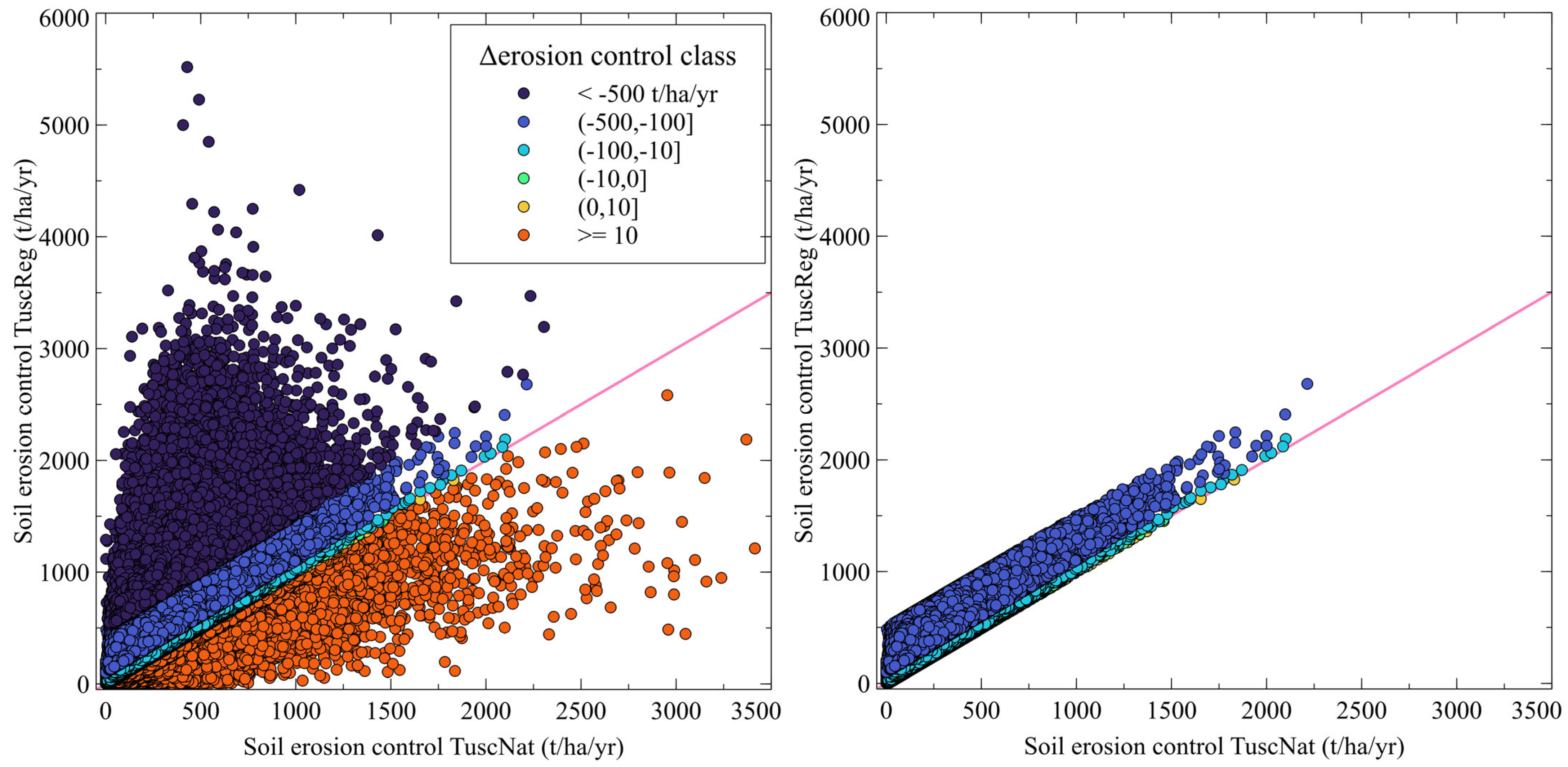
Overall, erosion control estimates between the two assessments were generally coherent (linear relation) across Δerosion control classes (Figure 7). However, for the class where TuscNat >> TuscReg, the dispersion increased for high values of erosion control. Moreover, as the Δerosion control values became larger (e.g., for the lower than –500 class, i.e., where TuscReg >> TuscNat in erosion control), the Δerosion control relationship between the two assessments weakened (Figure 7). At the extreme Δerosion control values (TuscReg >> TuscNat in erosion control), the two assessments even became non-coherent.
Figure 7.
Coherence between soil erosion control differences (potential erosion–actual erosion calculated through RUSLE) in Tuscany estimated through either regionally based data (Tusked) or EU-based data (TuscNat). Classes in the legend are for Δerosion control classes (see main text for details). The right panel shows all Δerosion control classes, except those when either TuscNat − TuscReg < –500 Mg ha−1 yr−1 (i.e., TuscReg >> TuscNat) and when TuscNat − TuscReg >= 10 Mg ha−1 yr−1 (i.e., TuscReg >> TuscNat). The red line is the 1:1 line. All graph axes and Δerosion control values for the different classes are in Mg ha−1 yr−1.
3.4. Correlation Between the Difference in Erosion Products and Erosion Factors in the Soil Regions
Correlations between the differences in RUSLE factors (i.e., CTuscNat−CTuscReg) and differences in erosion estimations (i.e., AactTuscNat−AactTuscReg) identified the main drivers of discrepancies between assessments. In general, the differences in Aact were moderately correlated with the differences in the C factor, but they did not affect erosion control, which was mainly correlated with R and secondarily with LS, as it was for the difference in Apot (Table 5).
Table 5.
Pearson correlation coefficients (r) between the differences (diffs) in RUSLE factors between national and regional assessments and the assessment diffs for actual erosion, potential erosion, and erosion control. Correlation analysis was carried out within each soil region and at the regional level. Colors highlight the strength of the correlation: |r| < 0.1 → negligible; 0.1 ≤ |r| < 0.3 → weak; 0.3 ≤ |r| < 0.5 → moderate; 0.5 ≤ |r| < 0.7 → strong; |r| ≥ 0.7 → very strong (from yellow to brown for positive correlations; blue for negative ones).
Just as it was reported above for the C factor, the correlations between the assessments’ differences in Aact and the differences in the C factor were stronger in the SRs dominated by forests, namely, 78.2, corresponding to the chain of the Apennines; 60.41, the Apuan Alps; and 60.4, the hilly and mountainous ranges of central Tuscany. Regarding Apot (where the C factor is excluded from the calculations), the differences in the R factor between assessments seemed to have the highest impact on SR 78.2, the chain of the Apennines. On the other hand, differences in LS were strongly correlated with differences in Apot both for the lowland plains (SR 64.4) and Mount Amiata (56.1). These differences did not lead to different erosion classes. Differences in K moderately correlated with differences in Apot in SRs 60.7 (coastal plains) and 60.4 (hilly and mountainous ranges of central Tuscany).
Differences in erosion control followed the same Apot trend in terms of correlation with differences in RUSLE factors: in the SRs of mountains 78.2 and 60.41, differences in R showed the strongest correlation to differences in erosion control; in the plains of SRs 64.4 and 56.1, differences in LS had the strongest correlation; in the large heterogeneous central SR 60.4 and in the coastal plains of SR 60.7, both differences in the K factor and in LS showed correlation to differences in erosion control.
Graphical comparison and Pearson correlation coefficients (r) confirmed that the variation in erosion control mainly derived from Apot differences.
4. Discussion
Tuscany exhibits pronounced variability in soil erosion rates due to its highly heterogeneous geology, complex topography, and land use practices, and the interplay of clay-rich badlands, steep vineyards, and Apennine slopes creates distinct erosion hotspots, exacerbated by Mediterranean rainfall regimes and anthropogenic pressures. In this context, soil regions represent a useful tool for analyzing results within more homogenous lands for soil environmental drivers. The highly erodible clay badlands soils of the Crete Senesi in SR 61.3 exhibit some of Italy’s most severe erosion rates (10–50 Mg ha−1 yr−1, escalating to >100 Mg ha−1 yr−1 in active gullies [47]), where clay behavior and sparse vegetation accelerate rill and gully erosion. Slopes under viticulture in the sandy–limestone hills of Chianti in SR 78.2 experience moderate to high erosion (5–10 Mg ha−1 yr−1), occasionally exceeding 22 Mg ha−1 yr−1 due to sheetwash and tillage-induced compaction [48]. Erosion is locally amplified on gradients >15%, where bare inter-rows lack vegetative cover. Mountain forested areas in SR 78.2 retain soils effectively with erosion rate <1 Mg ha−1 yr−1, while pastures and deforested slopes can reach 5–15 Mg ha−1 yr−1, with landslides exceeding 50 Mg ha−1 [49,50]. Lower-energy environments such as the Maremma hills and coastal areas of SR 60.7 exhibit low erosion rates (2–6 Mg ha−1 yr−1), though intensive agriculture and extreme rainfall events exacerbate topsoil loss.
Such variability explains the differences between TuscNat and TuscReg at local scales. The differences in the erosion factors stem from variations in both the datasets and the interpolation algorithms, whose individual contributions cannot be separated. Resampling was done on homogeneous RUSLE layers. The original datasets used different base grain sizes, spanning from 10 to 500 m.
Regarding the R factor, we can interpret the main differences because of the different numbers and spatial distribution of weather stations. In TuscReg, the use of a spatial multiple linear regression calibrated on a large regional dataset (1403 pluviometric stations) captured local extremes better. In contrast, ESDAC modeled the R factor across the entire EU, offering a more generalized representation, unable to properly capture the local variability in Tuscany, particularly in the northern part of the region. Low spatial or temporal resolution data can lead to an underestimation of erosivity [51,52]. In the Italian context, Petroselli et al. [53] showed how empirical R formulas vary in accuracy depending on data quality, stressing the need for high-resolution precipitation data.
K factor differences were affected both by data inputs and algorithms, such as in Torri et al. [36] with TuscReg; whereas, for the TuscNat map, the authors used the Wischmeier and Smith [54] nomograph with the LUCAS dataset. The results show that TuscNat generally has higher K, suggesting that Torri et al. underestimate erodibility in mineral soils rich in organic carbon (e.g., forests). This discrepancy is especially noticeable in areas like Mount Amiata, Elba Island, the Apuan Alps, and the highest Apennine ridges (soil organic carbon > 2.5%, [37]) Our results on the difference between using Torri et al. [36] and Wischmeier and Smith [54] are in line with the literature on databases of European erodibility, which highlights the need to limit the application of K on soils rich in organic carbon (typical of forests). The previous literature [16] advises caution when applying K to soils rich in organic carbon.
The LS factor differences are minimal, consistent with using the same Desmet & Govers [29] algorithm via SAGA GIS, and they arise from DEM resolution (25 m TuscNat, 10 m TuscReg). A slightly higher LS in TuscReg may relate to source DEMs and algorithm parameters. Indeed, DEM resolution is known to have an impact on LS accuracy [24,55,56], and differences also occur when resampling DEMs to coarser grids [57,58].
The differences in C factor values between TuscNat and TuscReg seem to be due to two main sources. For land uses, where the C factor was calculated with the inclusion of the fractional vegetation cover of several land covers (e.g., the percentage of cover of forests, pastures, sparsely vegetated areas, vineyards, orchards, and olive groves in mixed pixels), the discrepancies were more pronounced. Although the minimum and maximum tabular C values for each land use/cover class—used to weigh the fractional cover—are identical in both TuscNat and TuscReg, the differences in fractional cover between the input layers used appear to have a major influence. The stark contrast in land cover resolution (100 m in TuscNat vs. 10 m in TuscReg) contributes to the differences. During the resampling process from 10 m to 100 m, land use classes not represented in the coarser resolution in the national assessment may still be considered in the regional assessment, particularly in complex and heterogeneous landscapes. This issue is less relevant in areas dominated by extensive and homogeneous land use patterns.
Overall, RUSLE factor differences cause notable variation in potential erosion and soil erosion control outputs; however, it is worth highlighting how soil erosion control has the potential to become an important soil-based ecosystem service indicator [21,59,60]. Our results on spatial similarity and the spatially explicit relationship between the two assessments support the idea that erosion control assessments are qualitatively similar if the differences in their constituent RUSLE factors remain under a certain limit. When discrepancies become too large, the assessments become unrelated (i.e., qualitatively different). In our case, this was the case in soil regions with complex landscapes with significant differences in the R (TuscReg >>> TuscNat) and K factors (TuscNat >>> TuscReg), suggesting that some attention should be paid to similar areas when using RUSLE-based indicators. Other studies have highlighted how differences in the scale of the spatial products used as inputs to derive soil properties and processes or ecosystem services can have significant effects on the final results [61,62,63]. Similarly, no simple rule explains how scale differences between TuscNat and TuscReg affect outputs. In the case of Hamel et al. [62] and Bagstad et al. [63], resampling the DEM used as input was associated with estimations of higher erosion rates in small synthetic watersheds and at regional scales, respectively. In our case, the effect of the original scale and interpolation method is likely to be context-dependent.
Overall, the significant differences in the results are due to multiple factors, notably the resampling of fine-resolution data to a coarser grid. The averaging may reduce the model’s ability to capture peaks and spatial discontinuities, leading to an under- or overestimation. Furthermore, since the RUSLE model is multiplicative, the error may have been propagated and amplified in the results. In particular, the C factor, having gone from a resolution of 10 m to 100 m, reduced the model’s ability to distinguish protective cover from exposed areas. This may underestimate the effect of protective cover in fragmented areas and overestimate it in agricultural or urbanized areas. Another limitation in using European data for regional evaluation lies in the use of estimation based on models fitted all over Europe. This condition implies the realistic possibility of missing the estimation of extreme local values, as it was for the R factor.
5. Conclusions
According to our analyses, the results show that the use of layers with poor detail leads to underestimates or overestimates of the erosion phenomenon, resulting in defining intervention strategies that are ineffective or inadequate to the real distribution and magnitude of the actual processes. This is particularly evident in areas with complex and fragmented landscapes (hilly and mountainous areas of Tuscany), where data aggregation can distort the representation of erosive factors, significantly influencing the erosion estimate.
In more detail, our results show that the differences between the two assessments based on regional and EU scale datasets were mainly affected by (i) differences in R factors in mountain SRs, where precipitation is very intense and European-scale models are unable to capture extreme values and (ii) differences in LS factors in plain SRs, even if erosion values are so low that this weight does not translate into changes in Aact classes or in soil erosion control. In the more heterogeneous SRs, differences in K factors also had importance in determining the differences between national and regional levels of erosion products.
There were significant differences found in the estimation of soil erosion between the two applications: one based on European-scale data and the other on regional-scale data. These highlight a critical aspect of the application of regulations such as the EU Soil Monitoring and Resilience Law [11], which is aimed at protecting and restoring soil health, ensuring sustainable soil use, as we believe that the effectiveness of soil protection policies and management measures strictly depends on the level of detail of the data used to describe the status of soil health indicators. Therefore, to ensure the effectiveness of actual and future directives addressing soil health, it is essential that the processing is conducted with data of adequate resolution, especially at local and regional levels. Only in this way will it be possible to develop targeted policies and actions for soil protection, based on an accurate and realistic analysis of the vulnerability of the territory.
The results of this study support CAP 2023–2027 implementation in Italy, where soil erosion is managed through Good Agricultural and Environmental Conditions (GAEC) standards and rural development measures in Tuscany. High-resolution regional modeling better identifies erosion-prone areas than continental-scale products, improving the targeting of conservation measures and informing soil health assessment under the EU Soil Monitoring and Resilience Law, which relies on scientific thresholds of tolerable soil loss to classify soils as healthy or unhealthy. Each MS, in compliance with the law, shall identify its own maximum value at a level that would not result in any damage to human health or to the environment. As for farmers, our results will enable more precise identification of vulnerable areas, easier compliance with CAP, better access to support schemes, and long-term soil fertility preservation.
Supplementary Materials
The following supporting information can be downloaded at https://www.mdpi.com/article/10.3390/land15030417/s1.
Author Contributions
Conceptualization, E.M.-R., G.B., L.G., R.L. and F.U.; methodology, E.M.-R., G.B., L.G., R.L. and F.U.; formal analysis, E.M.-R., G.B., L.G., R.L. and F.U.; data curation, E.M.-R., G.B., L.G., R.L. and F.U.; writing—original draft preparation, E.M.-R., G.B., L.G., R.L. and F.U.; writing—review and editing, E.M.-R., G.B., L.G., R.L. and F.U.; visualization, E.M.-R., G.B., L.G., R.L. and F.U.; project administration, R.L. and F.U.; funding acquisition, F.U. All authors have read and agreed to the published version of the manuscript.
Funding
This research was funded by the SERENA project. SERENA (Soil Ecosystem seRvices and soil threats modElling aNd mApping) is an EJP SOIL internal project. EJP SOIL has received funding from the European Union’s Horizon 2020 research and innovation program: Grant agreement No. 862695.
Data Availability Statement
Data supporting the reported results can be found at https://zenodo.org/records/13952098 (accessed on 20 February 2026) and https://doi.org/10.5281/zenodo.18588496 (accessed on 20 February 2026).
Acknowledgments
The authors wish to thank the three anonymous reviewers of this paper for providing constructive comments, which have contributed to the improvement of the published version.
Conflicts of Interest
The authors declare no conflicts of interest.
Abbreviations
The following abbreviations are used in this manuscript:
| Aact | Actual Soil Loss (Mg ha−1 yr−1) |
| Apot | Potential Soil Loss (Mg ha−1 yr−1) |
| ASTER | Advanced Spaceborne Thermal Emission and Reflection Radiometer |
| C | Cover Management RUSLE Factor |
| CAP | Common Agricultural Policy |
| DEM | Digital Elevation Model |
| EPSG | European Petroleum Survey Group (Coordinate Reference System Codes) |
| ESDAC | European Soil Data Centre |
| ETRS89 | European Terrestrial Reference System 1989 |
| EU | European Union |
| GAEC | Good Agricultural and Environmental Conditions |
| IPBES | Intergovernmental Science Policy Platform on Biodiversity and Ecosystem Services |
| K | Soil Erodibility RUSLE Factor |
| LAEA | Lambert Azimuthal Equal Area (Projection) |
| LS | Slope Length and Steepness RUSLE Factor |
| LUCAS | Land Use/Cover Area Frame Survey |
| P | Support Practices RUSLE Factor |
| R | Rainfall Runoff Erosivity RUSLE Factor |
| RUSLE | Revised Universal Soil Loss Equation |
| SAGA | System for Automated Geoscientific Analyses |
| SDGs | Sustainable Development Goals |
| SRTM | Shuttle Radar Topography Mission |
| SR | Soil Region |
| TuscNat | National Scale Application for Tuscany |
| TuscReg | Regional Scale Application for Tuscany |
| UNCCD | United Nations Convention to Combat Desertification |
| USDA | United States Department of Agriculture |
References
- Saljnikov, E.; Eulenstein, F.; Lavrishchev, A.; Mirschel, W.; Blum, W.E.H.; McKenzie, B.M.; Lilburne, L.; Römbke, J.; Wilke, B.-M.; Schindler, U.; et al. Understanding Soils: Their Functions, Use and Degradation. In Advances in Understanding Soil Degradation, Innovations in Landscape Research; Saljnikov, E., Mueller, L., Lavrishchev, A., Eulenstein, F., Eds.; Springer: Cham, Switzerland, 2022; pp. 1–42. [Google Scholar] [CrossRef] [Scilit]
- Montagne, D.; Scammacca, O.; Walter, C.; Cousin, I. The Concept of Ecosystem Services and Its Application to Soil. In Agricultural Soil Science; Wiley: Hoboken, NJ, USA, 2025; pp. 161–209. [Google Scholar]
- European Commission. Communication from the Commission to the Council, the European Parliament, the European Economic and Social Committee and the Committee of the Regions: Thematic Strategy for Soil Protection; European Commission: Brussels, Belgium, 2006.
- European Commission. EU Soil Strategy for 2030. Reaping the Benefits of Healthy Soils for People, Food, Nature and Climate. COM(2021) 699 Final; European Commission: Brussels, Belgium, 2021.
- Evangelista, S.J.; Field, D.J.; McBratney, A.B.; Minasny, B.; Ng, W.; Padarian, J.; Román Dobarco, M.; Wadoux, A.M.J.-C. Soil Security—Strategizing a Sustainable Future for Soil. Adv. Agron. 2024, 138, 1–70. [Google Scholar] [CrossRef] [Scilit]
- Panagos, P.; Montanarella, L.; Barbero, M.; Schneegans, A.; Aguglia, L.; Jones, A. Soil Priorities in the European Union. Geoderma Reg. 2022, 29, e00510. [Google Scholar] [CrossRef] [Scilit]
- Panagos, P.; Borrelli, P.; Poesen, J.; Ballabio, C.; Lugato, E.; Meusburger, K.; Montanarella, L.; Alewell, C. The New Assessment of Soil Loss by Water Erosion in Europe. Environ. Sci. Policy 2015, 54, 438–447. [Google Scholar] [CrossRef] [Scilit]
- Morgan, R.P.C. Soil Erosion and Conservation; Wiley-Blackwel: Hoboken, NJ, USA, 2005. [Google Scholar]
- FAO; ITPS. Status of the World’s Soil Resources (SWSR)—Main Report; Food and Agriculture Organization of the United Nations and Intergovernmental Technical Panel on Soils: Rome, Italy, 2015. [Google Scholar]
- Alewell, C.; Borrelli, P.; Meusburger, K.; Panagos, P. Using the USLE: Chances, Challenges and Limitations of Soil Erosion Modelling. Int. Soil Water Conserv. Res. 2019, 7, 203–225. [Google Scholar] [CrossRef] [Scilit]
- European Commission. Directive (EU) 2025/2360 of the European Parliament and of the Council of 12 November 2025 on Soil Monitoring and Resilience (Soil Monitoring Law). Off. J. Eur. Union 2025, L 336, 1–Xx. [Google Scholar]
- Renard, K.G.; Foster, G.R.; Weesies, G.A.; McCool, D.K.; Yoder, D.C. Predicting Soil Erosion by Water: A Guide to Conservation Planning with the Revised Universal Soil Loss Equation (RUSLE). Agriculture Handbook No. 703; US Department of Agriculture: Washington, DC, USA, 1997.
- Stein, A.; Riley, J.; Halberg, N. Issues of Scale for Environmental Indicators. Agric. Ecosyst. Environ. 2001, 87, 215–232. [Google Scholar] [CrossRef] [Scilit]
- Orgiazzi, A.; Ballabio, C.; Panagos, P.; Jones, A.; Fernández-Ugalde, O. LUCAS Soil, the Largest Expandable Soil Dataset for Europe: A Review. Eur. J. Soil Sci. 2018, 69, 140–153. [Google Scholar] [CrossRef] [Scilit]
- Panagos, P.; Van Liedekerke, M.; Jones, A.; Montanarella, L. European Soil Data Centre: Response to European Policy Support and Public Data Requirements. Land Use Policy 2012, 29, 329–338. [Google Scholar] [CrossRef] [Scilit]
- Panagos, P.; Meusburger, K.; Ballabio, C.; Borrelli, P.; Alewell, C. Soil Erodibility in Europe: A High-Resolution Dataset Based on LUCAS. Sci. Total Environ. 2014, 479–480, 189–200. [Google Scholar] [CrossRef] [Scilit]
- Vinci, I. Valutazione del Rischio d’Erosione per la Regione Veneto. Available online: https://geomap.arpa.veneto.it/documents/316#more (accessed on 10 February 2026).
- Staffilani, F. Carta dell’Erosione Idrica Attuale della Regione Emilia-Romagna. Note Illustrative; Direzione Generale Cura del Territorio e dell’Ambiente, Regione Emilia-Romagna: Bologna, Italy, 2019. Available online: https://mappegis.regione.emilia-romagna.it/gstatico/documenti/dati_pedol/NOTE_ILLUSTRATIVE_EROSIONE.pdf (accessed on 20 February 2026).
- Tiberi, M.; Bernacconi, C.; Ciabocco, G.; Maggiori, F. Carta del Rischio di Erosione Attuale della Regione Marche. Available online: https://www.regione.marche.it/portals/0/PSR_Marche/eventi/SoiLandPro.23.03.23/Carta_rischio_erosione.pdf (accessed on 20 February 2026).
- Visser, S.; Keesstra, S.; Ní Choncubhair, Ó.; Mulder, T.; Costantini, E.; Sousanna, J.F.; Chenu, C.; Kuikman, P.; Barron, J.; Halberg, N.; et al. Roadmap for the European Joint Program SOIL: Towards Climate-Smart Sustainable Management of Agricultural Soils. Proc. West. Mark. Ed. Assoc. Conf. 2019, 30, 89. [Google Scholar] [CrossRef] [Scilit]
- Cousin, I.; Ungaro, F.; Bispo, A.; Altobelli, F.; Asins-Velis, S.; Assennato, F.; Astover, A.; Ay, J.-S.; Besnault, A.; Bondi, G.; et al. Synthesis of SERENA Outcomes; Zenodo: Geneva, Switzerland, 2024. [Google Scholar] [CrossRef]
- Regione Toscana Piano di Indirizzo Territoriale Con Valenza di Piano Paesaggistico. Available online: https://www.regione.toscana.it/-/piano-di-indirizzo-territoriale-con-valenza-di-piano-paesaggistico (accessed on 5 August 2025).
- IUSS Working Group WRB. World Reference Base for Soil Resources 2014, Update 2015 International Soil Classification System for Naming Soils and Creating Legends for Soil Maps; FAO: Rome, Italy, 2015. [Google Scholar]
- Regione Toscana SIPT: Database Pedologico. Available online: https://www502.regione.toscana.it/geoscopio/pedologia.html (accessed on 5 August 2025).
- Costantini, E.A.C.; Fantappié, M.; L’Abate, G. Climate and Pedoclimate of Italy. In The Soils of Italy; Springer: Dordrecht, The Netherlands, 2013; pp. 19–37. [Google Scholar]
- Righini, G.; Costantini, E.E.A.; Sulli, L. La Banca Dati Delle Regioni Pedologiche Italiane. Boll. Soc. Ital. Sci. Suolo 2001, 50, 261–271. [Google Scholar]
- Renard, K.G.; Foster, G.R.; Weesies, G.A.; Porter, J.P. RUSLE: Revised Universal Soil Loss Equation. J. Soil Water Conserv. 1991, 46, 30–33. [Google Scholar] [CrossRef] [Scilit]
- Panagos, P.; Ballabio, C.; Borrelli, P.; Meusburger, K.; Klik, A.; Rousseva, S.; Tadić, M.P.; Michaelides, S.; Hrabalíková, M.; Olsen, P.; et al. Rainfall Erosivity in Europe. Sci. Total Environ. 2015, 511, 801–814. [Google Scholar] [CrossRef] [Scilit] [PubMed]
- Desmet, P.J.J.; Govers, G. A GIS Procedure for Automatically Calculating the USLE LS Factor on Topographically Complex Landscape Units. J. Soil Water Conserv. 1996, 51, 427–433. [Google Scholar] [CrossRef] [Scilit]
- Conrad, O.; Bechtel, B.; Bock, M.; Dietrich, H.; Fischer, E.; Gerlitz, L.; Wehberg, J.; Wichmann, V.; Böhner, J. System for Automated Geoscientific Analyses (SAGA) v. 2.1.4. Geosci. Model Dev. 2015, 8, 1991–2007. [Google Scholar] [CrossRef] [Scilit]
- Panagos, P.; Borrelli, P.; Meusburger, K. A New European Slope Length and Steepness Factor (LS-Factor) for Modeling Soil Erosion by Water. Geosciences 2015, 5, 117–126. [Google Scholar] [CrossRef] [Scilit]
- Panagos, P.; Borrelli, P.; Meusburger, K.; Alewell, C.; Lugato, E.; Montanarella, L. Estimating the Soil Erosion Cover-Management Factor at the European Scale. Land Use Policy 2015, 48, 38–50. [Google Scholar] [CrossRef] [Scilit]
- Panagos, P.; Borrelli, P.; Meusburger, K.; van der Zanden, E.H.; Poesen, J.; Alewell, C. Modelling the Effect of Support Practices (P-Factor) on the Reduction of Soil Erosion by Water at European Scale. Environ. Sci. Policy 2015, 51, 23–34. [Google Scholar] [CrossRef] [Scilit]
- Thornton, P.E.; Running, S.W.; White, M.A. Generating Surfaces of Daily Meteorological Variables over Large Regions of Complex Terrain. J. Hydrol. 1997, 190, 214–251. [Google Scholar] [CrossRef] [Scilit]
- Borselli, L.; Cassi, P.; Salvador-Sanchis, P.; Ungaro, F.; Menduni, G.; Brugioni, M.; Sulli, L.; Montini, G. Studio della Dinamica delle Aree Sorgenti Primarie di Sedimento Nell’area 712 Pilota del Bacino di Bilancino: PROGETTO BABI. Relazione Finale Attività di Progetto; Consiglio Nazionale delle Ricerche, Istituto di Ricerca per la Protezione Idrogeologica: Firenze, Italy, 2007. [Google Scholar]
- Torri, D.; Poesen, J.; Borselli, L. Predictability and Uncertainty of the Soil Erodibility Factor Using a Global Dataset. Catena 1997, 31, 1–22. [Google Scholar] [CrossRef] [Scilit]
- Gardin, L.; Lorenzetti, R.; Ungaro, F. Maps of Topsoil (0–30 cm) Properties of Tuscany (Italy); Zenodo: Geneva, Switzerland, 2024. [Google Scholar] [CrossRef]
- Zanchi, C.A. Influenza Dell’azione Battente Della Pioggia e Del Ruscellamento Nel Processo Erosivo e Variazioni Dell’erodibilità Del Suolo Nei Diversi Periodi Stagionali. Ann. dell’Istituto Sper. Studio Dif. Suolo Firenze 1983, 14, 347–358. [Google Scholar]
- Rodolfi, G.; Zanchi, C.A. Caratteristiche Fondamentali e Dinamica Del Paesaggio Dell’Appennino Tosco Romagnolo. Ann. dell’Istituto Sper. Studio Dif. Suolo Firenze 1983, 14, 289–336. [Google Scholar]
- Zanchi, C.A. Primi Risultati Sperimentali Sull’influenza Di Differenti Colture Nei Confronti Del Ruscellamento Superficiale e Dell’erosione. Ann. dell’Istituto Sper. Studio Dif. Suolo Firenze 1983, 14, 277–289. [Google Scholar]
- Bazzoffi, P.; Pellegrini, S.; Chisci, G.; Papini, R.; Scagnozzi, A. Erosione e Deflussi a Scala Parcellare e Di Bacino in Suoli Argillosi a Diversa Utilizzazione Nella Val d’Era. Agric. Ric. 1997, 11, 5–20. [Google Scholar]
- Zanchi, C.A.; Cecchi, S.; Napoli, M. La Carta Del Rischio Erosivo per l’uso Sostenibile Del Territorio Agricolo Del Chianti. In Agricoltura e Erosione del Suolo in Toscana; Bonari, E., Debolini, M., Eds.; Felici Editore: Pisa, Italy, 2010; pp. 91–134. [Google Scholar]
- Napoli, M.; Cecchi, S.; Orlandini, S.; Mugnai, G.; Zanchi, C.A. Simulation of Field-Measured Soil Loss in Mediterranean Hilly Areas (Chianti, Italy) with RUSLE. Catena 2016, 145, 246–256. [Google Scholar] [CrossRef] [Scilit]
- Hijmans, R.J. Terra: Spatial Data Analysis; The R-Universe Platform: Vienna, Austria, 2025. [Google Scholar]
- Geary, R.C. The Contiguity Ratio and Statistical Mapping. Inc. Stat. 1954, 5, 115. [Google Scholar] [CrossRef] [Scilit]
- Li, X.; Anselin, L. Rgeoda: R Library for Spatial Data Analysis; The R-Universe Platform: Vienna, Austria, 2025. [Google Scholar]
- Bazzoffi, P. Measurement of Rill Erosion through a New UAV-GIS Methodology. Ital. J. Agron. 2015, 10, 1–18. [Google Scholar] [CrossRef] [Scilit]
- Napoli, R.; Piccini, C.; Di Bene, C.; Farina, R.; Marchetti, A.; Gazzetti, C.; Sarandrea, P. Agricultural Activities Effects on Groundwater Contamination in a Nitrate Vulnerable Zone of Latina Province. Rend. Online Soc. Geol. Ital. 2017, 42, 46–49. [Google Scholar] [CrossRef] [Scilit]
- Segoni, S.; Tofani, V.; Lagomarsino, D.; Moretti, S. Landslide Susceptibility of the Prato–Pistoia–Lucca Provinces, Tuscany, Italy. J. Maps 2016, 12, 401–406. [Google Scholar] [CrossRef] [Scilit]
- Rosi, A.; Tofani, V.; Tanteri, L.; Tacconi Stefanelli, C.; Agostini, A.; Catani, F.; Casagli, N. The New Landslide Inventory of Tuscany (Italy) Updated with PS-InSAR: Geomorphological Features and Landslide Distribution. Landslides 2018, 15, 5–19. [Google Scholar] [CrossRef] [Scilit]
- Porto, P. Exploring the Effect of Different Time Resolutions to Calculate the Rainfall Erosivity Factor R in Calabria, Southern Italy. Hydrol. Process. 2016, 30, 1551–1562. [Google Scholar] [CrossRef] [Scilit]
- Fischer, F.K.; Winterrath, T.; Auerswald, K. Temporal- and Spatial-Scale and Positional Effects on Rain Erosivity Derived from Point-Scale and Contiguous Rain Data. Hydrol. Earth Syst. Sci. 2018, 22, 6505–6518. [Google Scholar] [CrossRef] [Scilit]
- Petroselli, A.; Apollonio, C.; De Luca, D.L.; Salvaneschi, P.; Pecci, M.; Marras, T.; Schirone, B. Comparative Evaluation of the Rainfall Erosivity in the Rieti Province, Central Italy, Using Empirical Formulas and a Stochastic Rainfall Generator. Hydrology 2021, 8, 171. [Google Scholar] [CrossRef] [Scilit]
- Wischmeier, W.H.; Smith, D.D. Predicting Rainfall Erosion Losses. A Guide to Conservation Planning. Agriculture Handbook No 537; U.S. Department of Agriculture: Washington, DC, USA, 1978.
- Wang, G.; Gertner, G.; Parysow, P.; Anderson, A. Spatial Prediction and Uncertainty Assessment of Topographic Factor for Revised Universal Soil Loss Equation Using Digital Elevation Models. ISPRS J. Photogramm. Remote Sens. 2001, 56, 65–80. [Google Scholar] [CrossRef] [Scilit]
- Matheus, F.D.; Angelo, E.S.; Jean, S.d.S. Effects of DEM Resolution on the RUSLE-LS Factor and Its Implications on Soil and Water Management Policies through the Land Cover Seasonality. Afr. J. Agric. Res. 2020, 16, 1755–1765. [Google Scholar] [CrossRef] [Scilit]
- Akhila, R.; Pramada, S.K. Suitability of Different Digital Elevation Models in the Estimation of LS Factor and Soil Loss. Environ. Monit. Assess. 2025, 197, 511. [Google Scholar] [CrossRef] [Scilit]
- Delgado, D.; Sadaoui, M.; Ludwig, W.; Méndez, W. DEM Spatial Resolution Sensitivity in the Calculation of the RUSLE LS-Factor and Its Implications in the Estimation of Soil Erosion Rates in Ecuadorian Basins. Environ. Earth Sci. 2024, 83, 36. [Google Scholar] [CrossRef] [Scilit]
- Guerra, C.A.; Pinto-Correia, T.; Metzger, M.J. Mapping Soil Erosion Prevention Using an Ecosystem Service Modeling Framework for Integrated Land Management and Policy. Ecosystems 2014, 17, 878–889. [Google Scholar] [CrossRef] [Scilit]
- Paul, C.; Kuhn, K.; Steinhoff-Knopp, B.; Weißhuhn, P.; Helming, K. Towards a Standardization of Soil-related Ecosystem Service Assessments. Eur. J. Soil Sci. 2021, 72, 1543–1558. [Google Scholar] [CrossRef] [Scilit]
- Lemercier, B.; Lagacherie, P.; Amelin, J.; Sauter, J.; Pichelin, P.; Richer-de-Forges, A.C.; Arrouays, D. Multiscale Evaluations of Global, National and Regional Digital Soil Mapping Products in France. Geoderma 2022, 425, 116052. [Google Scholar] [CrossRef] [Scilit]
- Hamel, P.; Falinski, K.; Sharp, R.; Auerbach, D.A.; Sánchez-Canales, M.; Dennedy-Frank, P.J. Sediment Delivery Modeling in Practice: Comparing the Effects of Watershed Characteristics and Data Resolution across Hydroclimatic Regions. Sci. Total Environ. 2017, 580, 1381–1388. [Google Scholar] [CrossRef] [Scilit]
- Bagstad, K.J.; Cohen, E.; Ancona, Z.H.; McNulty, S.G.; Sun, G. The Sensitivity of Ecosystem Service Models to Choices of Input Data and Spatial Resolution. Appl. Geogr. 2018, 93, 25–36. [Google Scholar] [CrossRef] [Scilit]

Disclaimer/Publisher’s Note: The statements, opinions and data contained in all publications are solely those of the individual author(s) and contributor(s) and not of MDPI and/or the editor(s). MDPI and/or the editor(s) disclaim responsibility for any injury to people or property resulting from any ideas, methods, instructions or products referred to in the content. |
© 2026 by the authors. Licensee MDPI, Basel, Switzerland. This article is an open access article distributed under the terms and conditions of the Creative Commons Attribution (CC BY) license.