


Abstract
In regions where severe topographic constraints coincide with intensive human activity, the mechanisms underlying landscape ecological risk (LER) and its spatial differentiation remain poorly understood. In particular, the nonlinear responses and threshold effects arising from the combined influence of complex natural gradients, urban expansion, and policy interventions have not been adequately characterized, limiting effective regional ecological management and policy formulation. Taking the Taiyuan section of the Fen River Basin as the study area, this study constructed an LER index using land-use data for 2014, 2019, and 2024. Landscape metrics and spatial autocorrelation analyses were used to characterize the spatiotemporal evolution of LER, and a LightGBM-SHAP model with spatial block cross-validation was employed to identify the nonlinear effects of natural and socioeconomic drivers. A four-quadrant zoning framework integrating current risk state and driver sensitivity was then developed. The results showed that: (1) LER followed a fluctuating trajectory, rising from 2014 to 2019 and declining from 2019 to 2024, with evident spatial differentiation. Low- and relatively low-risk zones dominated about 71% of the area, while medium- to high-risk zones clustered mainly in the northeast, south, and parts of the northwest; high-risk agglomerations gradually contracted. (2) LER was driven by both natural and socioeconomic factors, with natural factors playing the stronger role. Slope, NDVI, elevation, and GDP were the key drivers. (3) The effects of these drivers were strongly nonlinear: slope increased risk at 5–13° but reduced it above 13°; NDVI displayed an inverted U-shaped relationship, with the strongest positive contribution at 0.60–0.75.; and elevation shifted from a positive to negative contribution near 1200 m. Based on these results, the framework coupling risk state and driver sensitivity delineated differentiated management units, providing fine-scale spatial guidance for ecological protection, restoration, and development control in topographically constrained river-valley basins.
1. Introduction
Under the combined pressures of global environmental change and rapid urbanization, land-use structures and landscape patterns are being continuously reorganized, exposing regional ecosystems to increasing fragmentation, functional degradation, and cumulative risk [1,2]. Human land-use activities not only alter land-use composition but also reshape landscape configuration and ecological processes, potentially undermining ecosystem stability and ecosystem-service provision while increasing ecological risk [3,4]. Landscape ecological risk (LER) represents the integrated potential for adverse ecological effects or damage arising from natural factors and human disturbances at a given regional scale [5]. LER indices translate spatial landscape characteristics into quantitative measures, thereby capturing landscape heterogeneity within a study area [6]. The resulting assessments provide an important basis for ecological protection, restoration, and spatial regulation [7,8]. LER assessment has been widely applied at watershed [9] and urban [10,11] scales. In practice, however, zoning approaches based solely on a single risk assessment are inherently static and outcome-oriented; consequently, areas with similar risk levels but different underlying mechanisms may be assigned to the same management category [12,13].
Recent studies have increasingly examined the determinants and spatial differentiation of LER and proposed differentiated management strategies tailored to specific drivers [5,14,15]. In ecologically fragile areas, mountainous watersheds, and arid regions, natural background conditions often shape the fundamental spatial pattern of LER [15,16]. In areas subject to intensive development and land use, human activities tend to determine the rate, direction, and spatial concentration of risk increases [17,18]. In regions with relatively unconstrained terrain, LER more commonly exhibits continuous clustering and accumulation or transitions from medium-low to higher risk levels [19,20]. Nevertheless, because environmental conditions and the intensity of human activity vary among regions, both the mechanisms and spatial patterns of LER differ substantially [5,21]. Particularly complex trajectories are likely where natural constraints and anthropogenic disturbance are strongly intertwined [22,23].
Drivers influence land-use transitions, landscape reconfiguration, and spatial aggregation, thereby generating the spatiotemporal differentiation of LER [24]. Rigorous attribution analysis is therefore essential for identifying priorities for spatial management. Common approaches include linear statistical models, such as ordinary least squares (OLS), in which model coefficients are used to interpret the effects of individual drivers [20]. Spatial attribution methods, including geographical detectors, geographically weighted regression (GWR) [25,26], and multiscale geographically weighted regression (MGWR) [27,28], have also been used to identify risk sources and spatial heterogeneity and to support ecological protection planning [29]. However, conventional spatial statistical models generally require prespecified functional forms or emphasize the effects of individual factors, limiting their ability to capture complex mechanisms [23]. LightGBM, by contrast, can efficiently represent nonlinear relationships and high-order interactions between environmental factors and LER, improving the identification of risk-driving processes [30]. When coupled with SHAP, it also quantifies the magnitude and direction of each factor’s contribution, thereby enabling interpretable analysis of LER formation mechanisms [31].
Overall, previous studies have developed differentiated strategies for managing regional landscape risk by examining natural and socioeconomic drivers and their spatial heterogeneity [21,32,33]. Analytical frameworks have expanded from single to multiple factors, with recent research explicitly considering interactions among drivers [34]. Methodological approaches have likewise progressed from simple linear models to machine-learning algorithms capable of capturing nonlinear relationships and high-order interactions [35,36]. Nevertheless, the mechanisms and spatial differentiation of ecological risk remain insufficiently understood in areas where strong topographic constraints coincide with intensive human activity. In particular, nonlinear responses and threshold effects arising from the combined influence of complex natural gradients, urban expansion, and policy interventions have yet to be fully characterized. Moreover, most existing studies focus either on risk patterns or on attribution alone and lack a framework that directly links LER assessment and driving mechanisms to spatial management. This gap limits the translation of research findings into fine-scale territorial governance [37].
Accordingly, this study uses the Taiyuan section of the Fen River Basin as a representative topographically constrained river-valley area. It constructs an LER assessment system, applies an interpretable LightGBM-SHAP framework to identify nonlinear driving mechanisms and interactions, and integrates these results with spatial zoning to develop a management framework that couples risk state with driver sensitivity. The study aims to provide methodological support and decision-making evidence for ecological-risk identification and differentiated spatial governance in complex terrain. Specifically, the objectives are to: (1) characterize land-use change, landscape-pattern evolution, and the spatiotemporal differentiation of LER in the Taiyuan section of the Fen River Basin from 2014 to 2024; (2) identify the dominant drivers of LER using LightGBM-SHAP and clarify the nonlinear responses and interactions of slope, NDVI, elevation, GDP, and other factors; and (3) integrate current LER with the contribution intensity of its drivers to delineate differentiated management zones and propose corresponding governance strategies.
2. Materials and Methods
2.1. Study Area
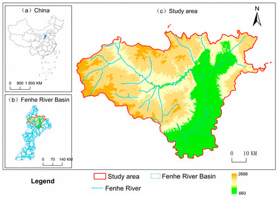
The Taiyuan section of the Fen River Basin was selected as the study area because it typifies a region in which strong topographic constraints coincide with intensive human activity. It lies between 37°27′–38°15′ N and 111°30′–113°01′ E (Figure 1) and encompasses a major part of Taiyuan, the capital of Shanxi Province. The area has a semi-humid continental monsoon climate, with mean annual precipitation of approximately 569 mm, mean annual evapotranspiration of approximately 450 mm, and a mean annual temperature of 8.1 °C. Precipitation is strongly seasonal, and droughts occur relatively frequently. Mountains cover approximately 65% of the study area, while the Fen River flows through its central valley. The natural gradient is pronounced: high mountains surround the basin, and the river valley extends longitudinally through its interior. The terrain can be broadly divided into three zones: high-elevation mountains, hilly transition zones, and the Fen River valley. Topographic and hydrological constraints concentrate human activities and urban development within the relatively narrow valley. In recent years, Taiyuan has undergone rapid development and economic transition as a resource-based city, intensifying competition for scarce land and increasing pressure for urban expansion. The study area therefore represents a typical coupled system in which a resource-based city intersects with an ecologically fragile region [36]. Its closely interwoven mountain–river–city pattern provides a suitable setting for examining interactions between natural and socioeconomic drivers.
Figure 1.
Location of the study area. (a) Shanxi Province, China; (b) the Fen River Basin; and (c) the Taiyuan section of the Fen River Basin.
2.2. Data Sources
The land-cover data comprised the 30 m annual China Land Cover Dataset (CLCD) developed by Xin Huang’s team at Wuhan University [38]. The dataset (Table 1) comprises nine land-use types: cropland, forest, shrubland, grassland, water bodies, snow and ice, bare land, wetlands, and impervious surfaces. All classes were used in the study area except for snow and ice and wetlands. Then we reclassified these land types into six land-use categories: cropland, forest land, grassland, water bodies, construction land, and unused land. The LightGBM–SHAP model was employed to analyze nine selected influencing factors: the normalized difference vegetation index (NDVI), precipitation, elevation (DEM), slope, population density, gross domestic product (GDP), distance to water bodies, distance to roads, and distance to towns (Table 1). Bilinear interpolation was used for continuous data, while nearest-neighbor interpolation was used for categorical data. ArcMap 10.8 was used to clip the land-cover and driving-factor datasets, transform them to a common coordinate system (WGS 1984 UTM Zone 49 N), and align their spatial extents. This preprocessing ensured that all raster layers had identical numbers of rows and columns, and perfectly aligned pixel grids, enabling accurate cell-by-cell spatial analysis.
Table 1.
Data sources.
2.3. Analytical Framework
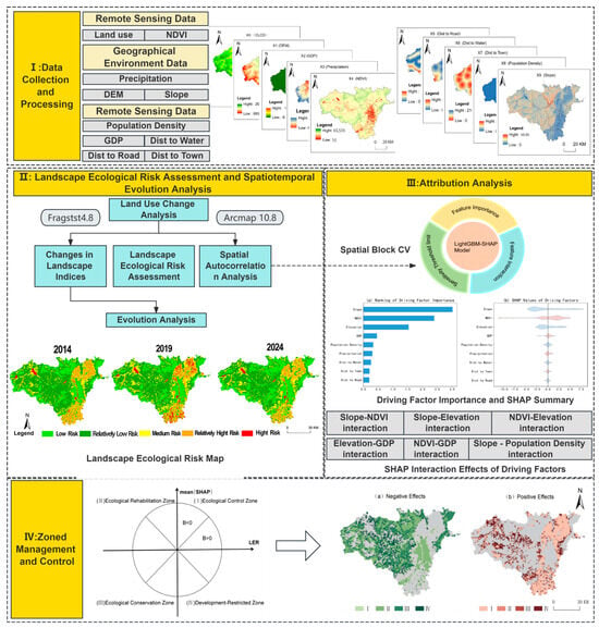
The analytical workflow integrated remote-sensing (Figure 2), environmental, and socioeconomic data to assess changes in LER and delineate differentiated territorial management zones. First, land-cover data were reclassified into six land-use categories, and land-use change was analyzed. A set of evaluation grids was then established to calculate LER. Next, landscape metrics were computed in FRAGSTATS 4.8 to characterize changes in landscape patterns. Based on the 2024 LER assessment and spatial autocorrelation results, a LightGBM-SHAP model with spatial block cross-validation was fitted to improve the reliability of spatial modeling. SHAP was used to interpret the machine-learning model, rank the global importance of the drivers, and identify thresholds and interactions among the principal factors affecting LER. The local contributions of the dominant factors were aggregated to represent driver sensitivity in each grid cell. Finally, current LER and driver sensitivity were integrated in a four-quadrant framework to delineate differentiated management zones that account for both present risk and potential future change.
Figure 2.
Analytical framework of the study.
2.4. Landscape-Pattern Analysis and Landscape Ecological Risk Assessment
Drawing on previous studies, landscape-pattern change at the municipal scale was assessed from five dimensions: fragmentation, connectivity, shape complexity, spatial aggregation, and landscape heterogeneity. These dimensions help explain changes in landscape ecological risk (LER).
Five landscape metrics were selected. The number of patches (NP) represents the total number of patches and reflects landscape fragmentation. The percentage of like adjacencies (PLADJ) measures the proportion of adjacent cell pairs belonging to the same class. It reflects the aggregation and adjacency of similar patches. Fractal dimension (FRAC) indicates patch-shape complexity. Higher FRAC values represent more complex and irregular patch boundaries. The clumpiness index (CLUMPY) measures the aggregation or dispersion of patches of the same class. Higher values indicate greater aggregation. Shannon’s diversity index (SHDI) reflects the richness and evenness of landscape types. It is therefore used to represent landscape heterogeneity.
To obtain evaluation units that were both spatially informative and readily interpretable, the study area was divided into compact, equal-sized ecological-risk units. FRAGSTATS 4.8 was used to calculate the total landscape area and number of patches. To ensure that each spatial unit contained sufficient landscape information while maintaining an appropriate visualization scale, this study evaluated the robustness of grid-size selection through sensitivity analyses at three spatial resolutions—500 m, 700 m, and 900 m (Figure A1, Figure A2 and Figure A3). The overall LER gradients and principal spatial patterns were consistent across the three scales. A 700 m grid was therefore selected as a compromise between spatial resolution and computational efficiency. Specifically, 700 × 700 m cells were generated with reference to a scale of approximately five times the mean patch area in the study area [39]. The LER index was constructed following the approach described in [40].
where (Li) denotes the landscape fragmentation index; (Ji) is the landscape separation index; (Qi) represents the landscape dominance index; (ni) is the number of patches of landscape type (i); (Ai) is the area of landscape type (i) (m2); and (A) is the total landscape area. (Di) denotes the ratio of the number of quadrats in which landscape type (i) occurs to the total number of quadrats; (Si) represents the proportion of patches of landscape type (i) relative to the total number of patches; and (Oi) is the proportion of the patch area of landscape type (i) relative to the total quadrat area. (Yi) and (Wi) denote the landscape loss index and landscape vulnerability index, respectively, while LER represents the landscape ecological risk index. The parameters (a), (b), and (c) are the weights assigned to the landscape fragmentation, separation, and dominance indices, respectively, satisfying (a + b + c = 1), and were set to 0.5, 0.3, and 0.2, respectively. (Mi) characterizes the degree to which a landscape type is affected by natural processes or human activities. The landscape vulnerability index (Wi) measures the extent to which a landscape type is susceptible to structural damage and functional degradation under external disturbances, as well as its difficulty in recovering from such disturbances. The landscape ecological risk index (LER) is an effective indicator for identifying regional ecological risks and evaluating regional ecological security.
Landscape ecological vulnerability refers to the relative susceptibility of different land-use types to structural degradation, loss of ecological functions, and difficulty in returning to their original state when subjected to the same degree of landscape disturbance. A higher value indicates greater landscape vulnerability and, consequently, a higher level of ecological risk [41]. Landscape vulnerability was assigned through expert judgment. Riverine water bodies are generally fragmented, and their shorelines are affected by development, reclamation, and encroachment, which amplify ecological risk; they were therefore assigned a vulnerability score of 5. Unused land has limited ecological recovery capacity and was assigned a score of 6. Cropland can partially mitigate risk under active management and was assigned a score of 4. Urban and industrial-mining land was considered structurally stable and was assigned the lowest score (1). Forest land and grassland received intermediate scores of 2 and 3, respectively. Thus, vulnerability scores for cropland, forest land, grassland, water bodies, urban and industrial-mining land, and unused land were 4, 2, 3, 5, 1, and 6, respectively [42]. The assigned scores represent ordinal and relative vulnerability coefficients rather than directly measured ecological quantities. Their purpose is to distinguish the relative susceptibility of land-use types within a unified LER framework. The score sequence and relative spacing were established by combining the ecological characteristics described above with scoring schemes used in previous landscape ecological risk studies. Because the vulnerability weights were largely determined through expert judgment, their assignment could substantially affect the resulting landscape ecological risk index. Therefore, a sensitivity analysis was conducted using Spearman’s rank correlation coefficient, in which the weight of each individual influencing factor was increased and decreased by 20%. As shown in Table 2, all correlation coefficients exceeded 0.96 and were statistically significant at the 0.01 level (p < 0.01), indicating a strong positive correlation between the adjusted and original results. These findings suggest that the landscape ecological risk assessment results are robust and insensitive to moderate variations in weight assignment.
Table 2.
Evaluation of LER sensitivity based on Spearman’s correlation analysis.
To examine changes in LER classes from 2014 to 2024, the assessments for 2014, 2019, and 2024 were classified using the Jenks natural breaks method. The three years were pooled before classification, and a common set of five thresholds was applied to all years to ensure consistent and reliable interannual comparisons.
2.5. Analysis of the Drivers of Landscape Ecological Risk
2.5.1. Spatial Autocorrelation Analysis
Spatial autocorrelation analysis was conducted to characterize the spatial clustering of LER and to determine whether spatial blocking was required to avoid attribution bias in the LightGBM-SHAP model (Section 2.5.2). Spatial autocorrelation measures the similarity of a variable across locations and thus quantifies the degree to which attribute values cluster among spatial units [43]. Moran’ s I includes both global and local statistics. Global Moran’s I was used to assess overall spatial dependence, whereas local Moran’s I identified local clusters and spatial outliers by measuring the association between each grid cell and its neighbors. These results also informed the spatial-blocking design used in subsequent modeling. The calculations followed the method of Anselin [44].
2.5.2. LightGBM-SHAP Attribution Analysis
To characterize complex relationships between natural and socioeconomic factors and LER, this study employed LightGBM. LightGBM is a high-performance gradient-boosting framework and an efficient implementation of gradient-boosted decision trees (GBDT). The model has an additive structure: its final prediction is the sum of the outputs from multiple decision trees [45]. This structure enables LightGBM to capture nonlinear responses and high-order interactions among multiple drivers of LER.
The model was trained by minimizing a specified loss function, L_ (y, Fz(x)), where y denotes the observed value and F(x) the ensemble prediction [46]. At iteration t, a new weak learner ℎt (x) was fitted to the prediction error of the current ensemble, Ft-1(x). The algorithm approximates the steepest-descent direction using the negative gradient of the loss function with respect to Ft-1(x), yielding the pseudo-residual rti. The calculations followed the method of Friedman [47].
Model predictive performance was evaluated using the root mean square error (RMSE) and coefficient of determination (R2), calculated as described in [48].
Prior to model construction, multicollinearity among the candidate influencing factors was assessed using the variance inflation factor (VIF). Variables with VIF values greater than 5 were excluded to reduce the potential influence of intervariable collinearity on model interpretation. Missing values in the influencing factors were imputed using the median. To minimize the interference of extreme values on model fitting, samples with landscape ecological risk values below the 1.5th percentile or above the 98.5th percentile were removed. All spatial datasets were projected to the WGS 1984 UTM Zone 49N coordinate system, with planar coordinates expressed in meters.
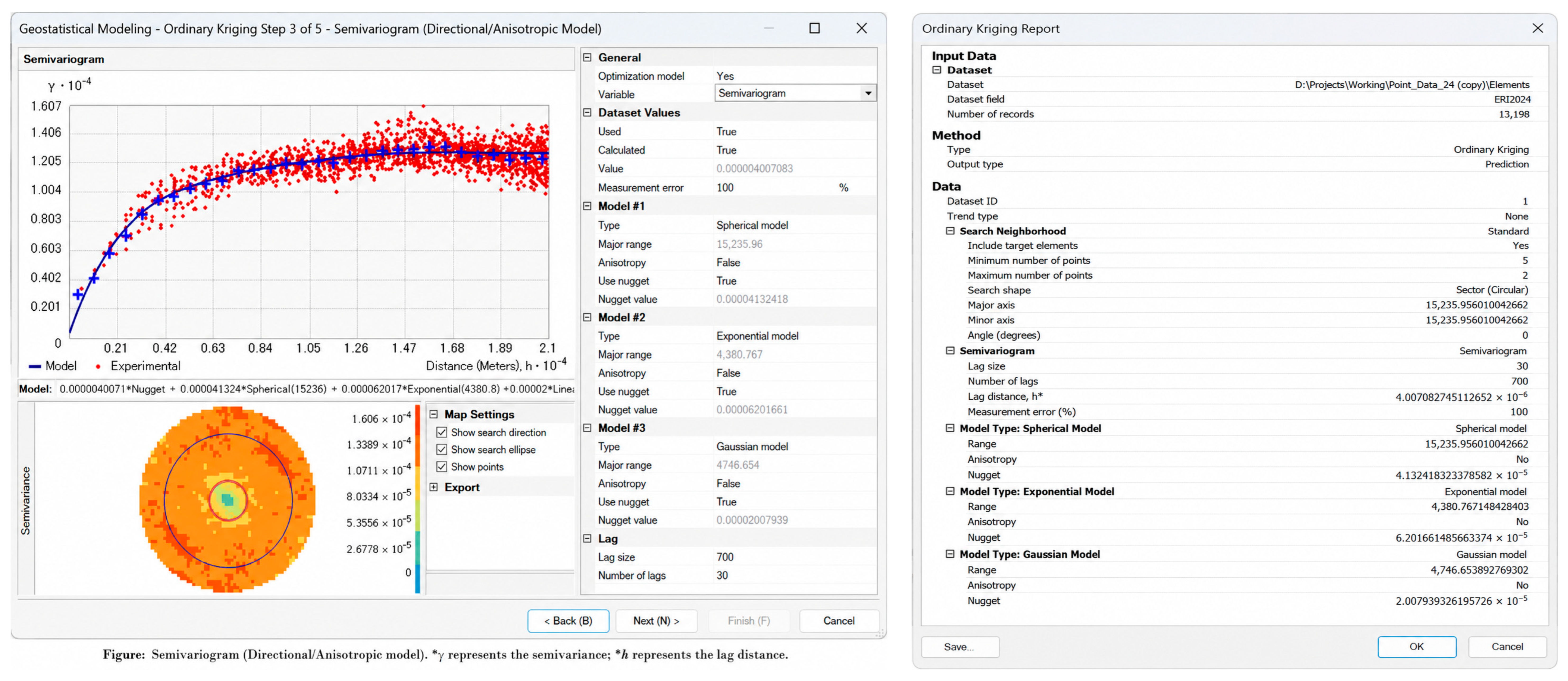
The Light Gradient Boosting Machine (LightGBM) model was constructed using the gradient boosting decision tree algorithm. The objective was specified as regression, and the root mean square error (RMSE) was used as the evaluation metric during model training. The main hyperparameters were set as follows: the maximum number of leaves was 63, the maximum tree depth was 10, the learning rate was 0.02, the feature sampling fraction was 0.80, and the sample subsampling fraction was 0.80. Sample resampling was performed every five boosting iterations. The minimum number of samples per leaf was set to 15, and both the L1 and L2 regularization coefficients were set to 0.1. The maximum number of boosting iterations was set to 3000. Early stopping was applied when the validation-set RMSE failed to improve for 150 consecutive iterations. The random seed was fixed at 42 to enhance the reproducibility of the results. Model performance was evaluated using the coefficient of determination (R2) and RMSE, and the means and standard deviations obtained from 5-fold spatial cross-validation were reported. To prevent spatial clustering from inflating model accuracy, we set the spatial blocking distance to 15,400 m based on the long-range variogram range, which represented the maximum distance of significant spatial autocorrelation.
SHAP is a model-interpretation framework that quantifies the contribution of each feature to an individual prediction and provides intuitive, consistent explanations of complex nonlinear models [49]. Coupling SHAP with LightGBM enabled the contributions of natural and socioeconomic conditions to predicting LER to be quantified and the principal underlying mechanisms to be identified.
The 2024 LER value for each 700 × 700 m grid cell served as the response variable. The predictor matrix comprised nine drivers: slope, elevation (DEM), NDVI, GDP, population density, distance to water bodies, distance to roads, distance to towns, and mean annual precipitation. Samples were first partitioned spatially into an 80% training set and a 20% independent test set. Based on the spatial autocorrelation results (Section 2.5.1), an appropriate block size and blocking scheme were selected, after which 5-fold spatial block cross-validation was conducted within the training set. This design reduced spatial information leakage and the overestimation of model performance arising from spatial autocorrelation, thereby improving the reliability of the spatial modeling results.
3. Results
3.1. Land-Use and Landscape-Pattern Changes
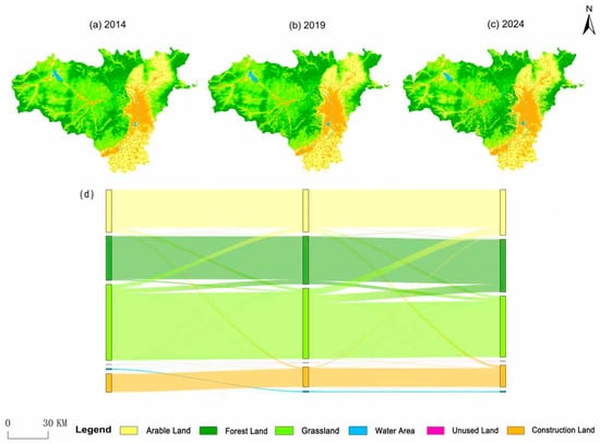
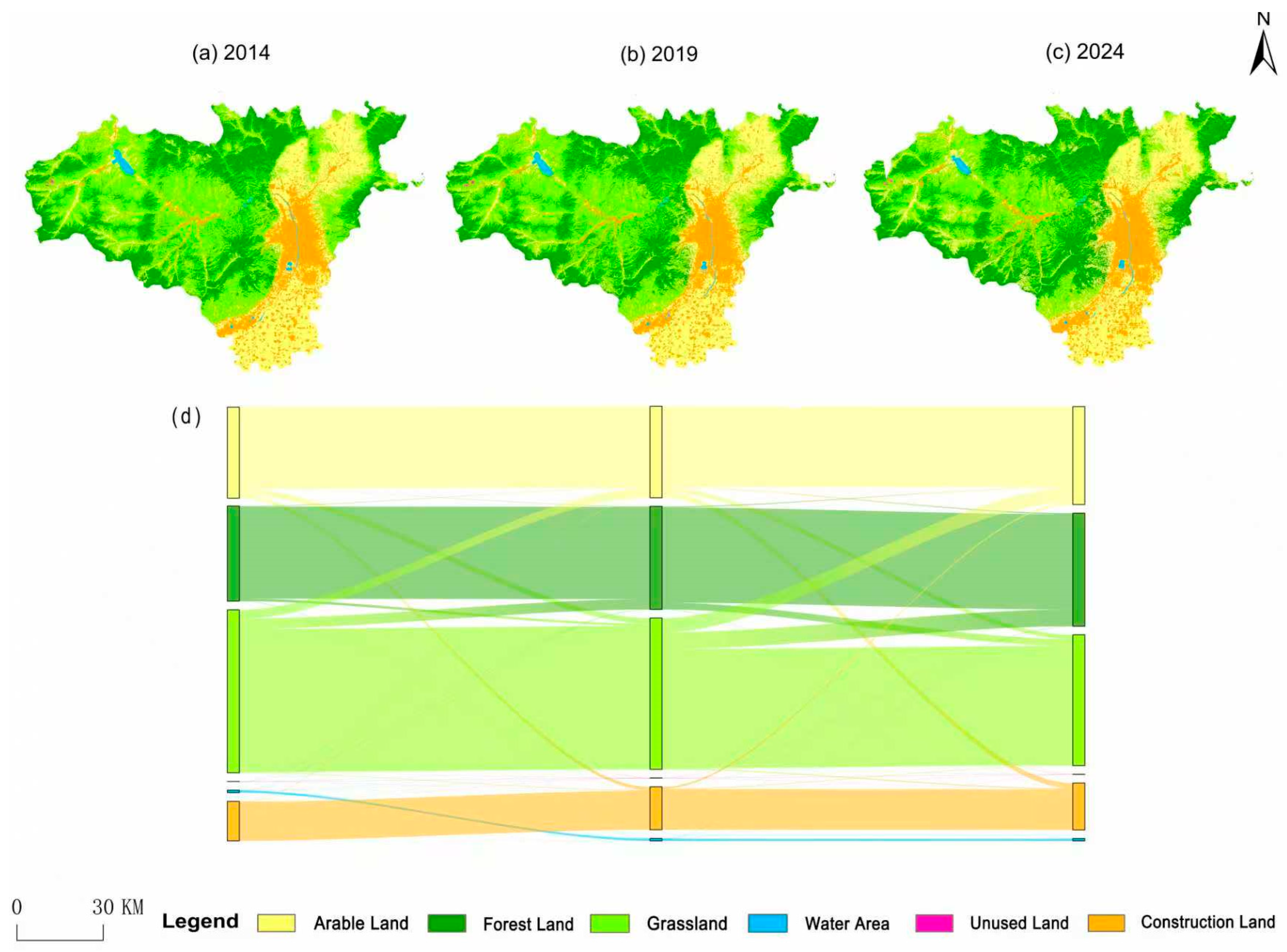
Forest land and grassland were the dominant land-use types throughout 2014–2024 (Figure 3). Together, they covered more than 62% of the study area, indicating a high overall level of vegetation cover. Grassland was the single largest category, accounting for more than 33% of the total area.
Figure 3.
Land-use distribution and transitions from 2014 to 2024. (a) 2014; (b) 2019; (c) 2024; and (d) Sankey diagram of land-use transitions between 2014 and 2024.
Land use changed substantially between 2014 and 2024. The areas of forest land, urban and industrial-mining land, and cropland increased, whereas grassland, water bodies, and unused land declined. Forest expansion occurred mainly through the conversion of grassland, representing approximately 1.70% of the total study area. Growth in urban and industrial-mining land occurred primarily at the expense of cropland (approximately 2.14%), while cropland expansion mainly replaced grassland (approximately 4.87%). The principal losses in grassland, water bodies, and unused land were therefore associated with conversion to forest land, cropland, and grassland, respectively. Forest land showed the largest net increase and accounted for 29% of the study area in 2024, with most of the gain originating from grassland.
Changes in the landscape metrics (Table 3) indicate an initial increase in fragmentation followed by landscape integration, together with a gradual increase in diversity. NP first increased and then decreased. Between 2014 and 2019, NP rose from 63,100 to 68,032 (7.8%), indicating intensified fragmentation, potentially associated with urban development and the conversion of grassland to forest land. Between 2019 and 2024, NP fell to 57,825 (15.0%), suggesting a subsequent reduction in fragmentation, possibly related to forest restoration and larger-scale land consolidation. Over the full decade, PLADJ and CLUMPY changed by only approximately 0.03% and remained close to 90, indicating consistently high aggregation among similar landscape types. FRAC increased slightly (0.44%) from 2014 to 2019 and then declined by 2.97% from 2019 to 2024. Patch shapes therefore became less complex overall, shifting from irregular and fragmented forms toward more regular and integrated configurations. SHDI increased continuously, increasing by 3.34% over the decade, indicating greater landscape diversity and potentially enhanced resistance to external disturbance.
Table 3.
Landscape metrics in the Taiyuan section of the Fen River Basin from 2014 to 2024.
3.2. Landscape Ecological Risk Assessment
LER values were classified into five levels: low risk (LER ≤ 0.024), relatively low risk (0.024 < LER ≤ 0.033), medium risk (0.033 < LER ≤ 0.042), relatively high risk (0.042 < LER ≤ 0.051), and high risk (LER > 0.051). The maps for 2014, 2019, and 2024 were spatially overlaid to construct transition matrices for 2014–2019, 2019–2024, and 2014–2024.
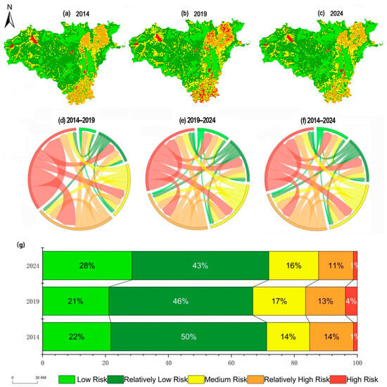
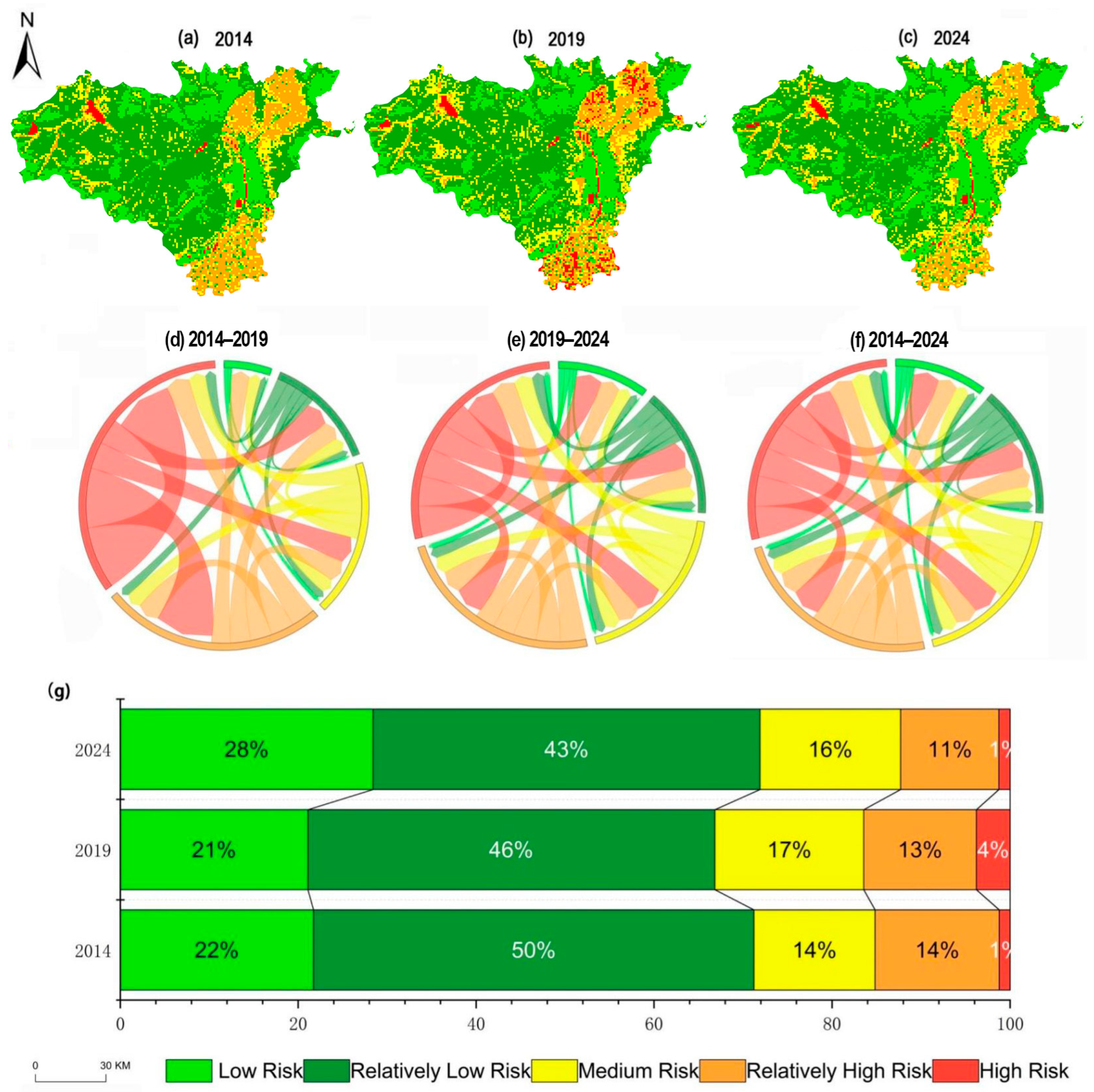
From 2014 to 2024, the distribution of LER classes followed a fluctuating trajectory (Figure 4), with the largest changes occurring in the low- and relatively low-risk zones. Low-risk zones decreased slightly and then expanded sharply; medium- and high-risk zones increased initially and subsequently declined; and relatively low-risk zones decreased continuously. Nevertheless, low- and relatively low-risk zones together accounted for 71% of the study area and remained the dominant classes. The expansion of low-risk zones was especially pronounced between 2019 and 2024, when their area increased by 457.90 km2, equivalent to 7.3% of the study area. Over the full decade, the share of relatively low-risk zones declined by 6%; approximately 422 km2 shifted from relatively low to low risk, indicating an overall improvement in ecological conditions. Medium-risk zones fluctuated, with approximately 216.59 km2 transitioning to relatively low risk. Relatively high-risk zones decreased by 2.92%, primarily through conversion to medium risk. High-risk zones expanded substantially from 2014 to 2019, reaching 3.79% of the study area, but had largely returned to their 2014 extent by 2024.
Figure 4.
Spatial distribution and transitions of LER in the Taiyuan section of the Fen River Basin, 2014–2024. (a–c) LER distributions in 2014, 2019, and 2024; (d–f) chord diagrams of LER transitions during 2014–2019, 2019–2024, and 2014–2024; and (g) area shares of the five LER classes.
3.3. Spatial Attribution of Landscape Ecological Risk
3.3.1. Spatial Autocorrelation Analysis
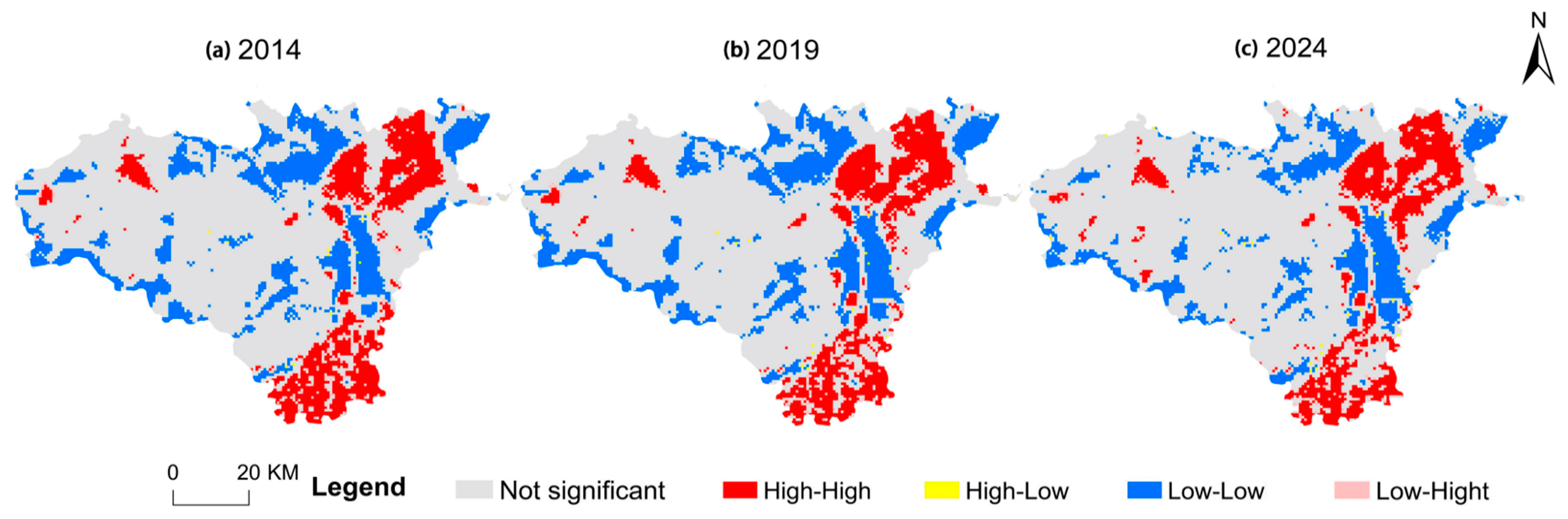
Global and local Moran’s I statistics were calculated to assess the spatial clustering of LER in 2014, 2019, and 2024. As shown in Table 4, global Moran’s I values were 0.184, 0.203, and 0.134, respectively. The corresponding z-scores and p-values indicated significance at the 99% confidence level, confirming positive spatial autocorrelation and significant clustering of LER. The local indicators of spatial association (LISA) maps (Figure 5) were dominated by high–high and low–low clusters, both of which were spatially concentrated and relatively stable. High–low and low–high outliers were rare and scattered. The number of high–high cells declined by 179 over the study period, indicating weaker clustering and a contraction of high-risk agglomerations. High–high clusters occurred mainly in cropland. Because cropland often adjoins urban land, it is susceptible to urban encroachment, has relatively low structural stability, and can readily be converted to urban and industrial-mining land. The number of low–low cells increased slightly and then declined markedly, with a net decrease of 387 cells, indicating reduced persistence of low-risk clusters. Low–low clusters were concentrated in forest land and urban and industrial-mining land. The latter is relatively stable because conversion costs are high and replacement by other land-use types is uncommon. Forest land, however, is vulnerable to conversion to cropland, which may explain the gradual decline in forest-dominated low–low clusters.
Table 4.
LISA cluster types for LER (number of grid cells).
Figure 5.
Spatial clusters of LER from 2014 to 2024. (a) 2014; (b) 2019; and (c) 2024.
3.3.2. Dominant Drivers of Landscape Ecological Risk
Because LER in the Taiyuan Basin is shaped by both topographic constraints and urban expansion, LightGBM-SHAP was used to identify complex nonlinear relationships and potential thresholds, particularly for slope, NDVI, and elevation. Based on the short and second-longest ranges of the semivariogram (Figure A4), the spatial block side length was set to 15,400 m, and five-fold spatial block cross-validation was performed. The data were split into training and test sets at an 80:20 ratio; outliers were removed, and missing values were imputed using the median to reduce distortion and improve predictive accuracy. Across the spatial cross-validation folds, the model achieved a mean R2 of 0.7805 ± 0.0272 and a mean RMSE of 0.0037 ± 0.0005, indicating strong explanatory performance for LER.
SHAP values from the fitted LightGBM model were then used to rank the drivers (Figure 6) and examine their nonlinear effects and interactions.
Figure 6.
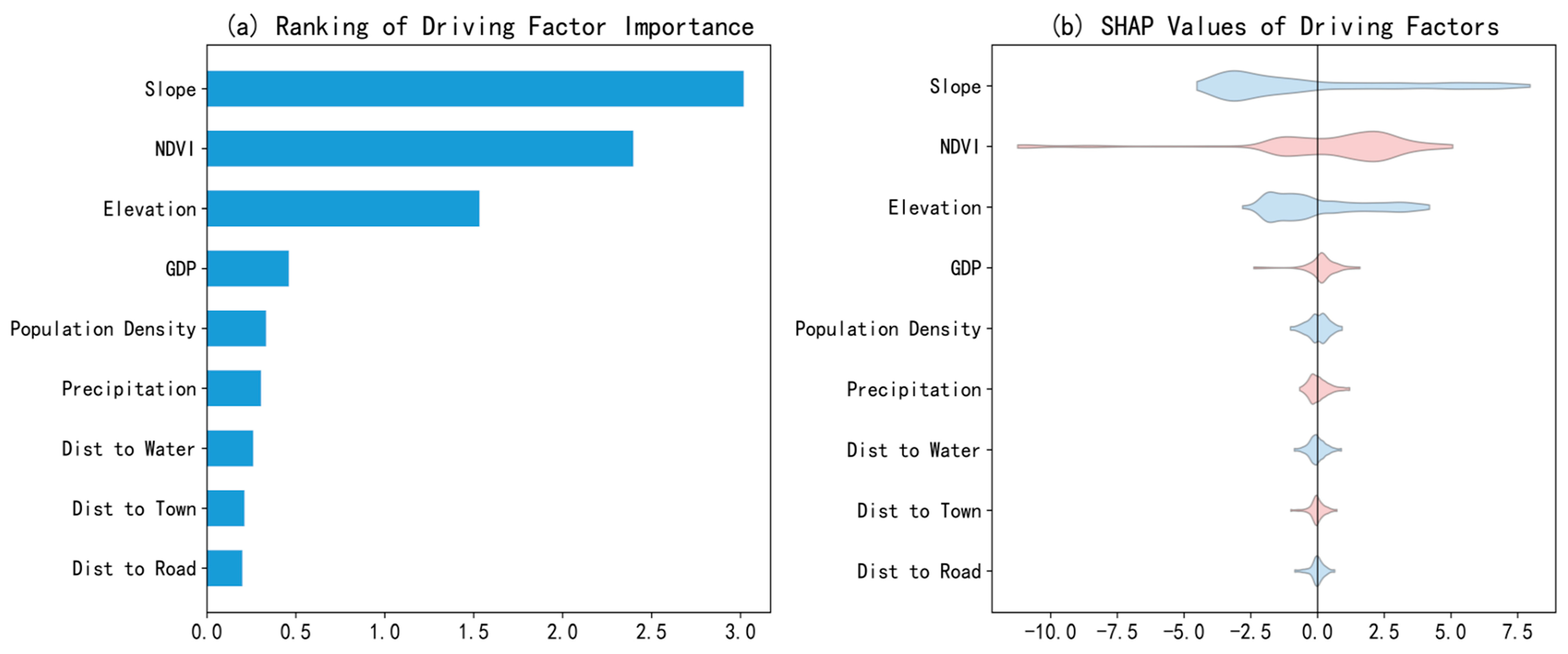
Importance of the drivers of LER. (a) Global importance ranking; and (b) distribution of SHAP values for each driver.
Global SHAP importance indicated that slope, NDVI, elevation, and GDP were the leading determinants of LER. Slope ranked first, underscoring the strong role of topographic conditions in shaping LER across the study area. Distance to roads had the lowest importance. Overall, natural factors exerted greater influence than socioeconomic factors.
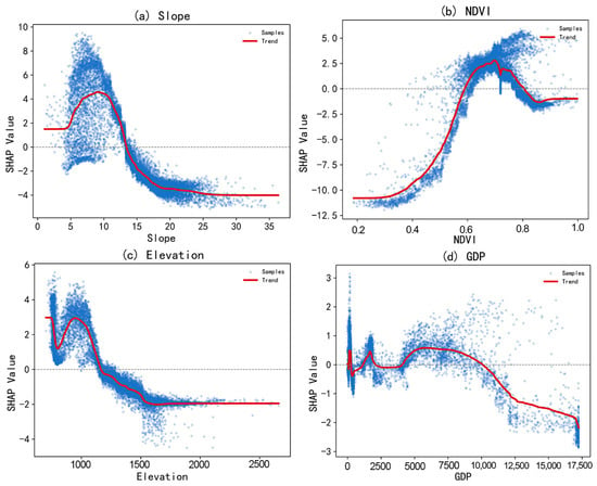
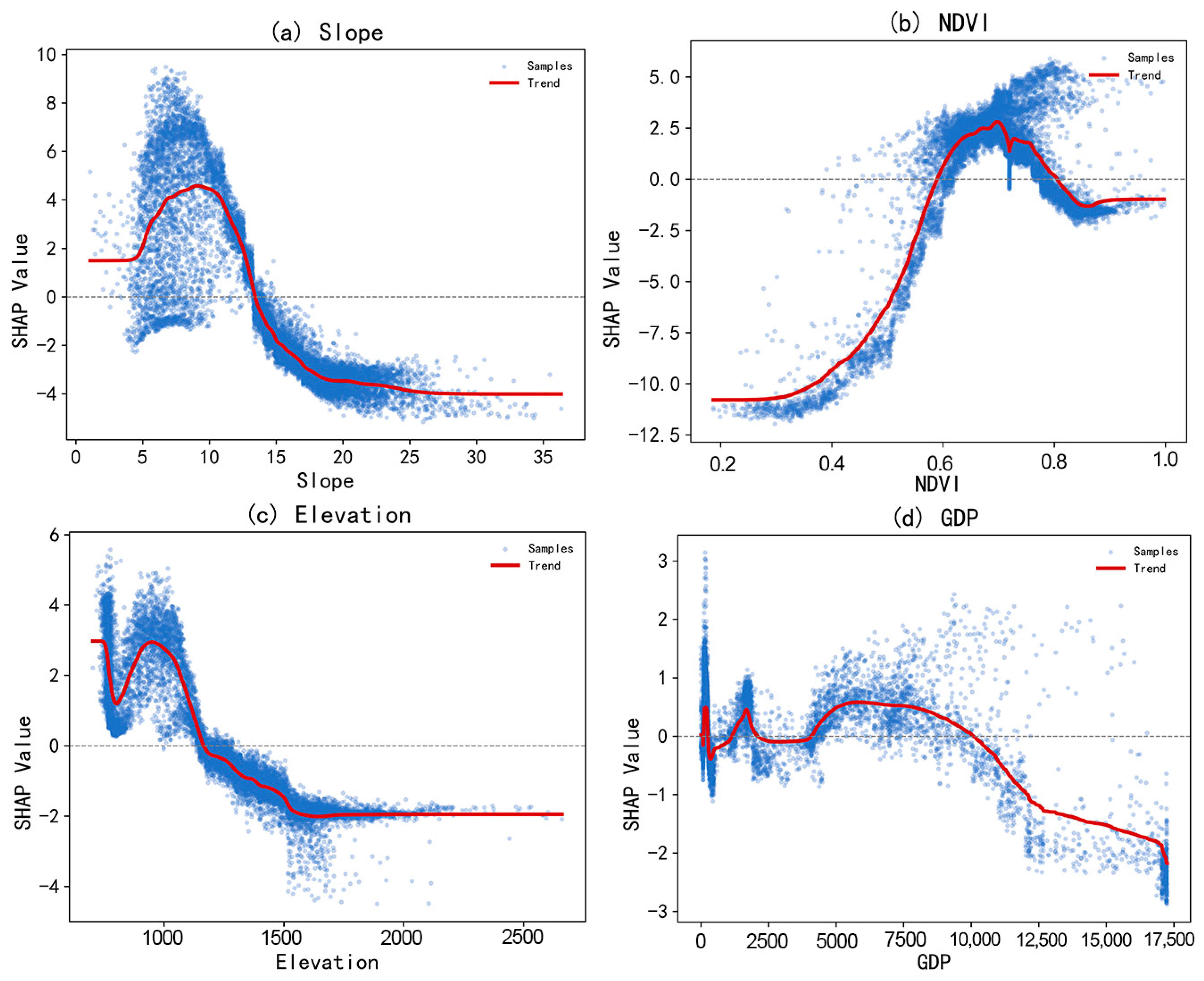
The SHAP-value distributions (Figure 7) differed markedly among drivers. A wider distribution indicates greater spatial variation in a driver’s effect and potentially more complex underlying processes. NDVI had the broadest distribution, including a pronounced negative tail, indicating that its relationship with LER was not monotonic; in some locations, higher vegetation cover substantially reduced risk. Slope and elevation also exhibited wide SHAP ranges, suggesting threshold behavior and interactions with land-use type and the intensity of human activity.
Figure 7.
Effects of individual drivers on LER. (a) Slope; (b) NDVI; (c) elevation and (d) GDP.
Slope exhibited a clear nonlinear relationship with LER. As slope increased, SHAP values generally rose and then declined. Between 5° and 13°, SHAP values were predominantly positive and highly dispersed, indicating that slopes in this range generally increased LER, although the magnitude varied among locations. Above 13°, SHAP values became mostly negative and more tightly clustered, suggesting that steeper terrain reduced LER by constraining human development and functioning as a topographic barrier.
NDVI displayed an approximately inverted U-shaped relationship with LER. SHAP values were predominantly positive at NDVI values of 0.60–0.75, indicating elevated risk within this intermediate range of vegetation cover. Areas with NDVI < 0.60 were generally urbanized or sparsely vegetated and had comparatively low modeled LER. At NDVI > 0.75, SHAP values generally declined; these areas typically corresponded to highly vegetated ecological spaces, such as forest land and nature reserves.
Elevation was negatively associated with LER overall, although the strength and direction of its effect varied across elevation bands. Below 1200 m, SHAP values were generally positive, indicating greater exposure to human disturbance and higher LER in low-elevation areas. As elevation increased beyond approximately 1200 m, SHAP values gradually shifted into the negative range. GDP also exhibited a nonlinear relationship with LER, but the pattern was less distinct than those for slope, NDVI, and elevation. Its contribution varied more widely among locations, indicating a more spatially heterogeneous and context-dependent mechanism.
3.3.3. Interactions Among the Dominant Drivers
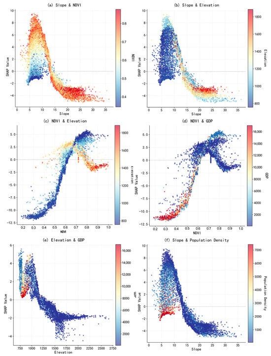
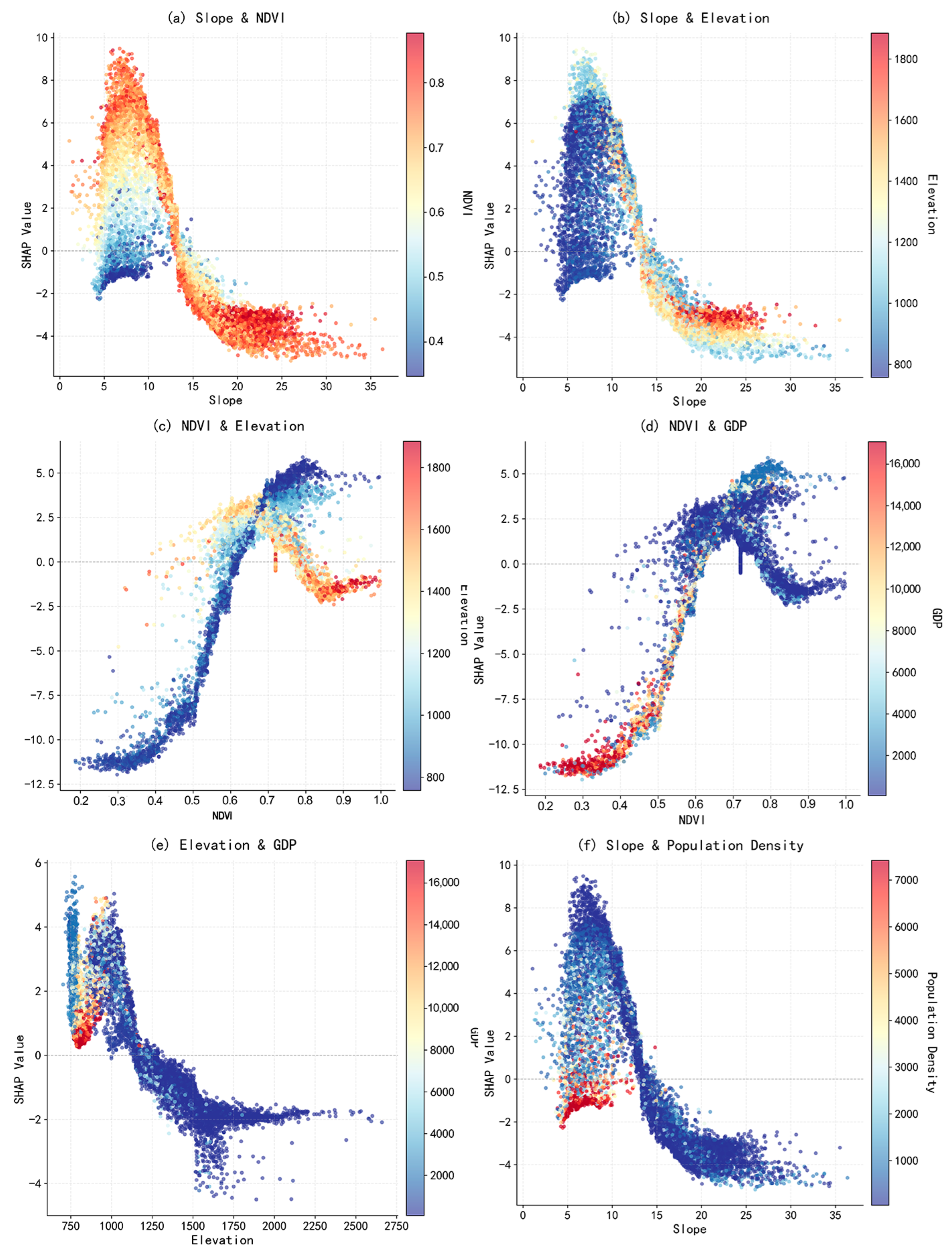
The effect of slope on LER was strongly nonlinear at lower gradients (Figure 8). SHAP values increased and reached a maximum between 0° and 8°, but then declined; above approximately 13°, they became negative and stabilized, indicating that steep terrain had a risk-reducing effect. High-elevation areas generally coincided with steeper slopes and also showed negative SHAP contributions, suggesting that the combination of high elevation and steep terrain constrains the expansion of human activity. Slope, elevation, and NDVI therefore did not act independently; together, they captured the influence of topographic constraints on human disturbance and landscape-pattern change.
Figure 8.
Pairwise interactions among the dominant drivers of LER. (a) Slope and NDVI; (b) slope and elevation; (c) NDVI and elevation; (d) NDVI and GDP; (e) elevation and GDP; and (f) slope and population density.
As NDVI increased from 0.20 to approximately 0.60, SHAP values rose from low levels and became positive, suggesting that increasing vegetation cover in low- to moderately vegetated areas was associated with landscape fragmentation, land-use transition, or changes in ecological space. At NDVI values above 0.80, however, SHAP values no longer increased monotonically and instead diverged according to elevation. In low-NDVI areas, high-elevation samples generally had higher SHAP values than low-elevation samples, whereas in high-elevation areas with very dense vegetation, SHAP values declined rapidly below zero, indicating that intact vegetation cover mitigated LER. High-GDP samples were concentrated mainly in low-NDVI areas and generally had negative SHAP values. Together, these patterns reveal the joint regulation of LER by vegetation, topography, and economic activity.
At elevations below 1200 m, SHAP values for elevation were positive, indicating that low-lying terrain generally increased LER. The values crossed zero and became negative as elevation rose, confirming a pronounced risk-reducing effect in high-elevation areas. Low-elevation (<1200 m), low-GDP locations made particularly large positive contributions to LER, likely reflecting extensive land expansion in economically less-developed plains and basin margins. In these areas, cropland and low-efficiency construction land strongly fragment natural patches, making the effect of elevation especially pronounced in low-lying terrain.
However, the contribution rate of GDP as a single factor does not differ markedly from those of the lower-ranked factors. Moreover, the data points are widely scattered rather than concentrated around the trend line, indicating that the variation is characterized by considerable specificity and complexity, with no clear pattern available for further analysis. Therefore, no interaction analysis was conducted for GDP.
4. Discussion
By focusing on a topographically constrained river-valley region along a terrain–water–urban gradient, this study characterized the evolution of LER, identified nonlinear effects and interactions among its drivers, and translated the findings into differentiated spatial-management strategies.
4.1. Temporal Evolution of Landscape Ecological Risk
LER in the Taiyuan section of the Fen River Basin followed a nonmonotonic trajectory, increasing from 2014 to 2019 and declining from 2019 to 2024. The initial increase coincided with a 7.8% rise in NP and greater patch-shape complexity, consistent with rapid urban development, encroachment on ecological and agricultural land, and fragmentation of existing land-use types. During 2019–2024, LER decreased as NP fell by 15%, FRAC declined by approximately 3%, and landscape aggregation remained stable. Across the full decade, NP decreased by 8.36%, FRAC decreased by 2.54%, and SHDI increased by 3.34%, indicating a shift toward greater aggregation, a more regular spatial structure, and a more balanced composition of landscape types. Comparable studies have reported similarly fluctuating trajectories in LER associated with land-use change, including initial increases followed by declines in overall risk, low-risk areas that first contract and then expand, and medium- and high-risk areas that show the opposite pattern [36,50]. Research on urbanized watersheds has likewise demonstrated that rapid urbanization can substantially alter land-use structure and landscape configuration, with consequences for aquatic environments and ecological processes [20,51]. In light of municipal ecological-restoration initiatives and territorial spatial controls, the observed variation in LER may reflect a staged response to the combined effects of urban expansion, ecological restoration, and spatial regulation. However, the specific contribution of each process cannot be determined from the present analysis. In particular, it remains difficult to identify whether the observed land-cover transitions were primarily caused by the conversion of ecological or agricultural land to urban land, by restoration-induced changes in land cover, or by other forms of human disturbance. Consequently, although changes in landscape patterns and influencing factors were associated with temporal variations in LER, these relationships should not be interpreted as direct causal effects. The lack of direct data on land-use transition drivers, restoration activities, and policy implementation represents an important limitation of this study.
4.2. Spatial Differentiation and Its Evolution
LER fluctuated over the study period, but low- and relatively low-risk zones consistently dominated, together accounting for 71% of the study area and indicating generally stable landscape conditions. Several classes nevertheless changed substantially. High-risk zones expanded to 3.79% of the study area in 2019 but had returned to approximately their 2014 extent by 2024. Relatively low-risk zones contracted continuously, largely through transition to low risk, while low-risk zones expanded markedly between 2019 and 2024, by an area equivalent to 7.3% of the study area. Overall, these shifts indicate an improvement in ecological conditions. The large-scale conversion of grassland to forest land during 2019–2024 represented not only an increase in the area of ecological land but also a potential improvement in its quality. In zones where cropland and construction land were interspersed, the consolidation of small patches and increasing regularity of landscape patches associated with higher risk may reflect the effects of spatial planning and land management on otherwise spontaneous development.
LER also displayed pronounced spatial heterogeneity associated with the basin’s constrained terrain. Unlike a typical plain, the Taiyuan section is a topographically confined river-valley basin whose spatial structure is jointly shaped by the Lüliang Mountains, the Taihang Mountains, and the main channel of the Fen River. Development is concentrated on low-elevation, gently sloping land, while the river corridor further promotes the clustering of population, industry, and infrastructure. Consequently, the spatiotemporal evolution of LER followed a distinct terrain–water–urban gradient rather than a random pattern [28]. Low- and relatively low-risk zones were concentrated in high-elevation areas with dense vegetation and contiguous ecological land, where development costs are high, topographic barriers are strong, and ecological space remains comparatively intact. Relatively high- and high-risk zones, by contrast, were concentrated in the eastern valley and along the Fen River, where human disturbance is more intensive. The urban core divides the eastern valley and creates clear agro-urban transition zones to the north and south. Within the established urban area, land-use patterns are relatively stable and therefore less prone to abrupt change. The flatter northern and southern margins, however, combine high development suitability with severe land scarcity. Competition between cropland and construction land is consequently acute, patches are more fragmented, and landscape structure is less stable. These patterns directly link the basin’s terrain–water–urban configuration to LER and demonstrate how limited developable space intensifies land-use conflict. By altering landscape configuration, such conflicts can undermine ecosystem stability and ecosystem-service provision, thereby increasing LER. Previous studies have similarly linked landscape fragmentation, patch aggregation, and shape complexity to ecosystem stability and LER [14,21], and have shown that intense land-use conflict can substantially elevate ecological risk [52].
4.3. Nonlinear Driving Mechanisms and Threshold Effects
The threshold and stage-dependent responses identified here show that LER evolution in river-valley basins is not a simple cumulative process but is governed by nonlinear feedbacks. Slope, elevation, and NDVI ranked well above GDP, population density, and distance to roads, indicating that natural conditions remain the primary determinants of spatial variation in LER in topographically constrained basins. By contrast, studies of rapidly urbanizing watersheds without strong topographic constraints have identified human disturbance and socioeconomic factors, such as GDP, as dominant drivers [53]. The difference suggests that, in basins with strong natural constraints, mountains, rivers, and urban space jointly structure the LER pattern, giving slope, NDVI, and elevation greater explanatory power. Socioeconomic factors remain relevant, but their effects are more localized and weaker at the regional scale.
The effects of these natural conditions were nevertheless strongly nonlinear. Slope contributed positively to LER between 5° and 13°, but its contribution declined rapidly above 13°; elevation exhibited a clear threshold at approximately 1200 m; and NDVI followed an inverted U-shaped response. These results demonstrate that LER is not aligned monotonically with either a single natural gradient or low-elevation urbanization [29]. High-elevation mountains are physically constrained but experience little human disturbance and therefore do not exhibit the highest risk. Conversely, although human activity is concentrated in the urban core, its land-use configuration is relatively stable, which limits LER. The highest risk instead occurred mainly in peri-urban transition zones and along the Fen River, indicating a pronounced urban-edge effect. Mountain–urban transition zones can accommodate cropland, grassland, and construction land simultaneously; the resulting mixture of landscape types, frequent land-use conversion, and high fragmentation promote risk accumulation. The river valley also has favorable environmental conditions and high potential vegetation cover, yet industrial production and residential activities are concentrated along the river corridor and depend heavily on its water resources. This concentration of disturbance helps explain the high-risk status assigned to water bodies. More broadly, the result underscores that land-use vulnerability in LER assessment is context dependent: the same land-use type can represent different ecological states in different settings. Previous studies likewise suggest that vegetation generally acts as a protective factor but can also indicate vulnerability during rapid landscape transformation [54].
4.4. Differentiated Spatial Management and Policy Implications
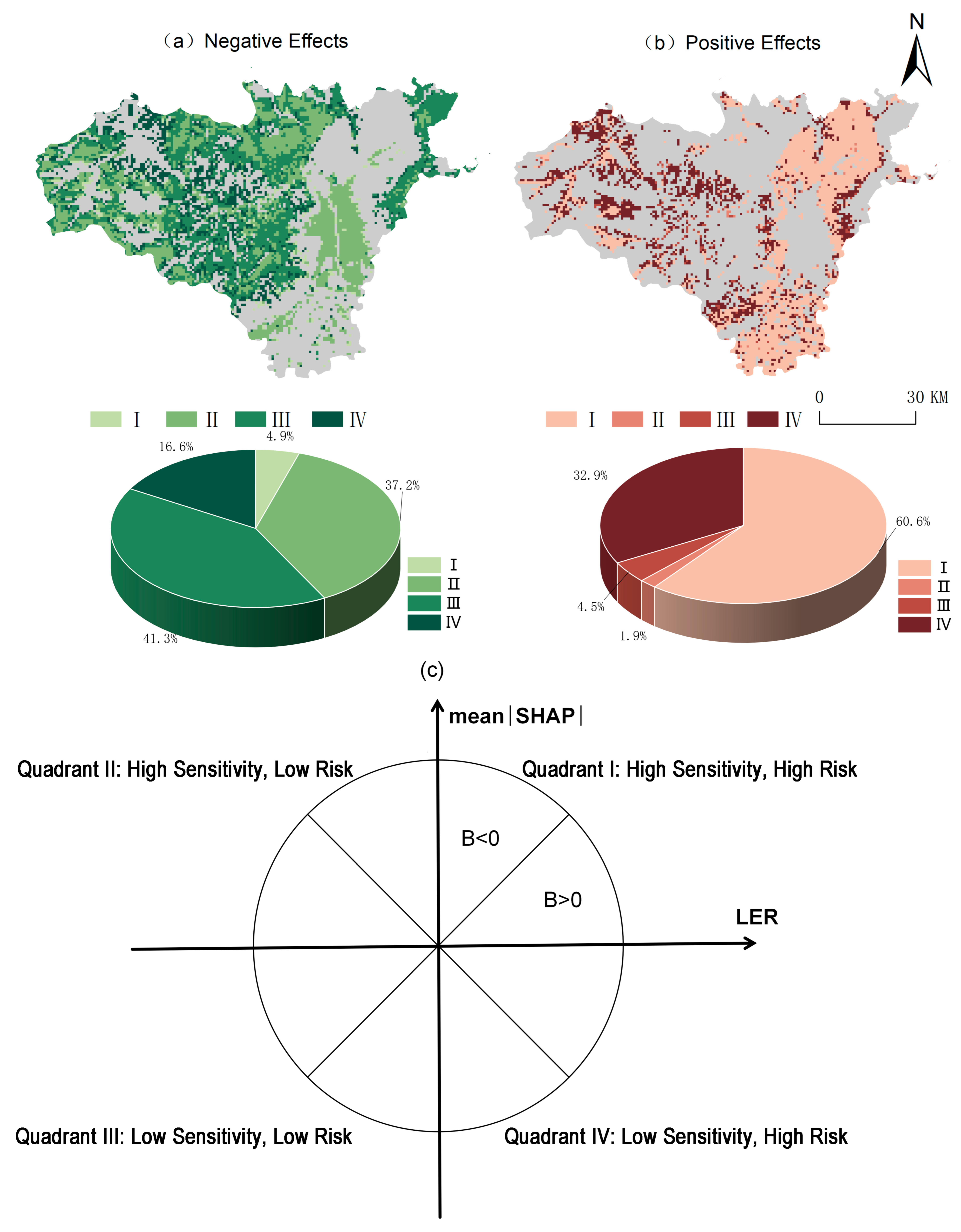
Given the spatial heterogeneity of landscape ecological risk, differentiated territorial spatial zoning and management were conducted based on landscape ecological risk. A 700 m × 700 m grid was used as the basic zoning unit. At the grid-cell scale, slope, elevation, and NDVI were selected as the primary influencing factors, and the median values of landscape ecological risk (LER) and the corresponding SHAP values were used as thresholds for the four-quadrant classification. The x-axis represents the LER value, reflecting the current state of landscape ecological risk, whereas the y-axis represents the mean absolute SHAP value (mean |SHAP|) of the dominant factors, indicating the sensitivity of risk to these drivers. A larger mean |SHAP| value suggests a greater likelihood that the underlying conditions of the dominant factors will induce changes in ecological risk. Accordingly, the current risk state and its driving sensitivity in 2024 can be integrated to anticipate future risk trends and formulate differentiated management strategies.
Quadrant I represents areas characterized by relatively high risk and substantial changes, whereas Quadrant II comprises areas with relatively low risk but substantial changes. Quadrant III includes areas with relatively low risk and limited changes, while Quadrant IV represents areas with relatively high risk but limited changes. To further distinguish the direction of these effects, Bi was introduced as an indicator of positive or negative effects. A value of Bi > 0 indicates a positive effect, whereas Bi < 0 indicates a negative effect.
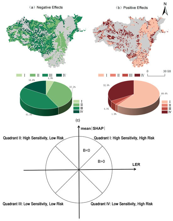
The results (Figure 9) show that negative effects accounted for 60.12% of the study area, while positive effects accounted for 39.88%. Despite being less dominant, positive effects still represented a substantial proportion, suggesting that the underlying natural conditions may increase landscape ecological risk across a considerable portion of the study area. Therefore, targeted policy interventions should be implemented in specific areas according to their corresponding land-use types to prevent further increases in landscape ecological risk.
Figure 9.
Spatial zoning of landscape ecological risk (LER) based on the current risk state and sensitivity to the dominant drivers in 2024. (a) Four-quadrant zoning under the negative effects of slope, elevation, and NDVI on LER (Bi < 0); (b) four-quadrant zoning under their positive effects on LER (Bi > 0); and (c) conceptual framework of the four-quadrant classification. Quadrants I–IV represent high risk–high sensitivity, low risk–high sensitivity, low risk–low sensitivity, and high risk–low sensitivity, respectively.
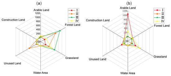
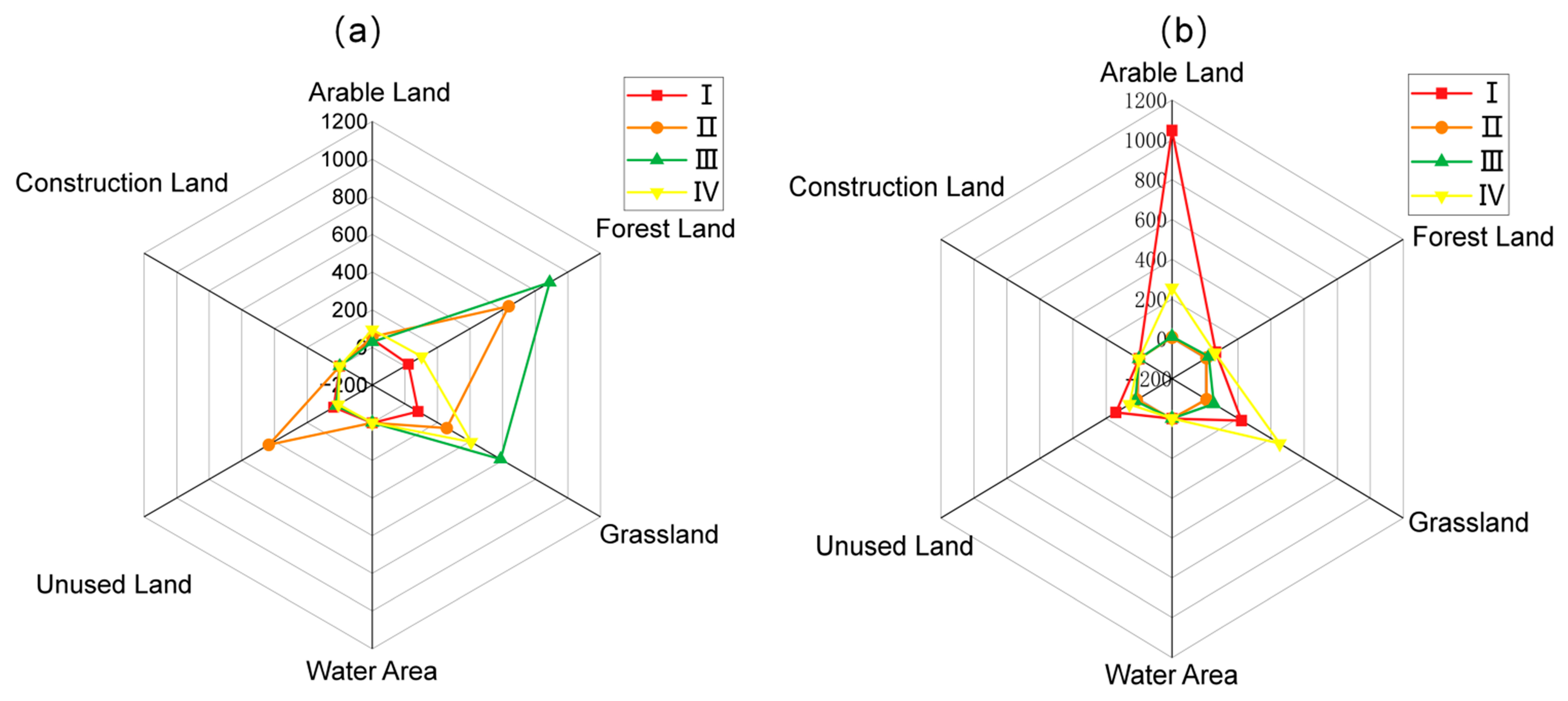
The positive and negative effects are shown in Figure 10. Under negative-effect driving conditions, Quadrants II and III accounted for relatively large proportions, indicating that low-risk areas were either stable or continuing to improve and therefore had the potential for further reductions in landscape ecological risk. Quadrant II was particularly prominent in forestland and built-up land, suggesting that ecological risk recovery primarily depended on these two land-use types. Quadrant III was mainly distributed across forestland and grassland, where landscape ecological risk remained low and generally stable. Quadrant IV was concentrated in some grassland areas characterized by relatively high ecological risk but slow recovery under the prevailing natural background conditions. Quadrant I represented the smallest proportion, indicating that areas with both high risk and favorable conditions for rapid recovery were relatively limited.
Figure 10.
Distribution of land-use types across the four risk–driver sensitivity quadrants under (a) negative effects (Bi < 0) and (b) positive effects (Bi > 0). Quadrants I–IV represent high risk–high sensitivity, low risk–high sensitivity, low risk–low sensitivity, and high risk–low sensitivity, respectively.
Under positive-effect driving conditions, Quadrants I and IV were dominant, together accounting for approximately 90% of the positively affected areas. This pattern indicates that high-risk areas followed two distinct trajectories: rapid change and relatively slow change. Quadrant I was mainly associated with cropland, where landscape ecological risk was high and likely to continue increasing in the future. Therefore, priority should be given to controlling risk increases caused by cropland conversion and other land-use changes. Quadrant IV was dominated by grassland and cropland. Although these areas also exhibited high risk levels, changes induced by the natural background conditions were relatively slow; nevertheless, the risk may still increase over time.
Conventional LER assessments usually delineate management zones directly from risk classes and are therefore outcome-oriented. Yet areas with the same risk level may arise from entirely different mechanisms, and risk class alone cannot support precise governance [55]. Nonlinear models provide a more realistic representation of these context-dependent processes. By linking LER assessment directly to territorial spatial regulation, the present framework improves attribution while generating differentiated management zones. The integrated assessment–attribution–management framework combines current outcomes and underlying mechanisms within common spatial decision units, shifting risk governance from static classification toward dynamic, driver-informed anticipation. From a spatial perspective, the four types of zones occupy distinct positions along the regional gradient. Forestland and grassland in Quadrant III under negative effects are primarily distributed within mountainous ecological barrier zones. Cropland in Quadrant I under positive effects is mainly located in urban–rural transition zones, whereas grassland in Quadrant IV is concentrated along the main stem of the Fen River and at the urban expansion frontier. Quadrant IV under positive effects and Quadrants II and IV under negative effects are often overlooked in conventional risk assessments. However, this study identifies these areas as priorities for forward-looking risk prevention and control, highlighting the value of the proposed framework in anticipating risk-driving processes and identifying potential ecological risks.
4.5. Limitations and Future Research
The LER index, derived from land-use patterns and landscape metrics, provides a systematic representation of spatial heterogeneity. However, although LightGBM-SHAP quantifies variable contributions to model predictions and reveals nonlinear associations, these explanations should not be interpreted as causal effects [31]. Future research should validate the identified mechanisms using field observations, data on policy implementation, and formal causal-inference methods. Moreover, this study characterized drivers based on current dominant factors but did not simulate future spatial scenarios under alternative policy pathways. Future work could couple SHAP-based attribution with scenario-based predictive models that explicitly incorporate planning and development policies, thereby better representing policy-regulated landscape change.
Further research is also needed to disentangle the terrain–water–urban gradient more explicitly. The nonlinear mechanisms identified in the Taiyuan section of the Fen River Basin may be transferable to other rapidly urbanizing regions subject to similar topographic constraints, although this proposition requires comparative validation. The results show that LER does not simply accumulate with increasing land-use intensity; it is also structured by gradients created by topographic barriers, the stability of established urban landscapes, and mixtures of competing land-use types. This perspective extends LER research in complex terrain. Methodologically, the framework advances spatial planning from static pattern assessment toward mechanism-based analysis and may also inform related analyses of ecological resistance and human disturbance. Overall, the study provides a more refined spatial basis for ecological protection, restoration, and development control.
5. Conclusions
Using the Taiyuan section of the Fen River Basin as a case study, this research developed an integrated assessment–attribution–management framework. LightGBM-SHAP was used to quantify the nonlinear contributions and interactions of natural and socioeconomic drivers of LER, and a four-quadrant approach was applied to delineate differentiated management zones. The principal conclusions are as follows:
- (1)
- Land use and landscape structure followed a fragmentation-to-integration trajectory. Between 2014 and 2024, forest land, urban and industrial-mining land, and cropland increased by 284.53 km2, 115.58 km2, and 106.72 km2, respectively, whereas grassland, water bodies, and unused land declined. NP increased from 2014 to 2019 and then decreased from 2019 to 2024, indicating that fragmentation first intensified and subsequently weakened. SHDI increased by approximately 3.3%, reflecting greater landscape diversity. Overall, the landscape shifted from a more irregular and fragmented configuration toward a more regular and integrated one.
- (2)
- LER exhibited a fluctuating temporal pattern and clear spatial differentiation. Low- and relatively low-risk zones dominated, covering 71% of the study area. Low-risk zones declined initially and then expanded sharply, including an increase of 457.90 km2 during 2019–2024; medium- and high-risk zones showed the opposite trajectory, while relatively high-risk zones declined continuously by 2.92%. Low- and relatively low-risk zones were concentrated mainly in the northern and central parts of the study area, whereas medium- and high-risk zones occurred primarily in the northeast, south, and a small area in the northwest. High-risk zones were closely associated with water bodies. Following ecological protection and restoration during 2019–2024, many higher-risk zones transitioned to lower-risk classes, indicating overall mitigation of LER.
- (3)
- Natural factors dominated the spatial differentiation of LER and exhibited pronounced nonlinear effects. The principal drivers ranked as follows: slope > NDVI > elevation > GDP. Slope increased LER primarily between 5° and 13° but reduced it below 5° and above 13°. NDVI followed an inverted U-shaped relationship, with the greatest positive contribution at 0.60–0.75, while elevation increased risk below approximately 1200 m and reduced it above this threshold. Interactions among the factors highlighted the constraint imposed by topography on human activity: risk was lowest in high-elevation areas with dense vegetation, whereas low-elevation, low-GDP areas made large positive contributions because of extensive land expansion.
- (4)
- Integrating current risk with driver sensitivity enabled more precise zoning and management. Landscape ecological risk in the study area was predominantly influenced by negative effects, accounting for 60.12%, with most areas exhibiting relatively low risk levels and trends toward stability or improvement. Positive effects accounted for 39.88% and were mainly concentrated in croplands along the urban fringe, areas along the Fen River, and urban expansion frontiers, where ecological risks were relatively high and showed an upward trend, thus requiring priority management. By integrating risk level, magnitude of change, and direction of influence, the “state–driver” zoning framework addresses the limitations of conventional risk-based zoning and facilitates differentiated and forward-looking management of landscape ecological risk.
Author Contributions
Conceptualization, J.L., X.F., and C.Z.; methodology, Y.Y., X.C., and X.Y.; validation, X.F.; formal analysis, J.L., Y.L., and C.Z.; investigation, J.L.; resources, C.Z.; data curation, Z.Z., Y.Y., and Y.M.; writing—original draft, J.L.; writing—review & editing, Y.L., C.Z., X.F., and J.L.; visualization, Y.Y., L.Z., and Y.L.; supervision, C.Z., X.F., and X.Y.; project administration, X.Y.; funding acquisition, C.Z., and X.F. All authors have read and agreed to the published version of the manuscript.
Funding
This research was funded by the National Natural Science Foundation of China (grant No. 42201298), the Shanxi Provincial Philosophy and Social Sciences Planning Project (grant No. 2025QN072), and the Scientific and Technological Innovation Foundation of Shanxi Agricultural University (Ph.D. Research Startup; grant No. 2022BQ10).
Data Availability Statement
The original contributions presented in this study are included in the article. Further inquiries can be directed to the corresponding author.
Conflicts of Interest
The authors declare no conflicts of interest. The funders had no role in the design of the study; in the collection, analyses, or interpretation of data; in the writing of the manuscript, or in the decision to publish the results.
Appendix A
Appendix A.1
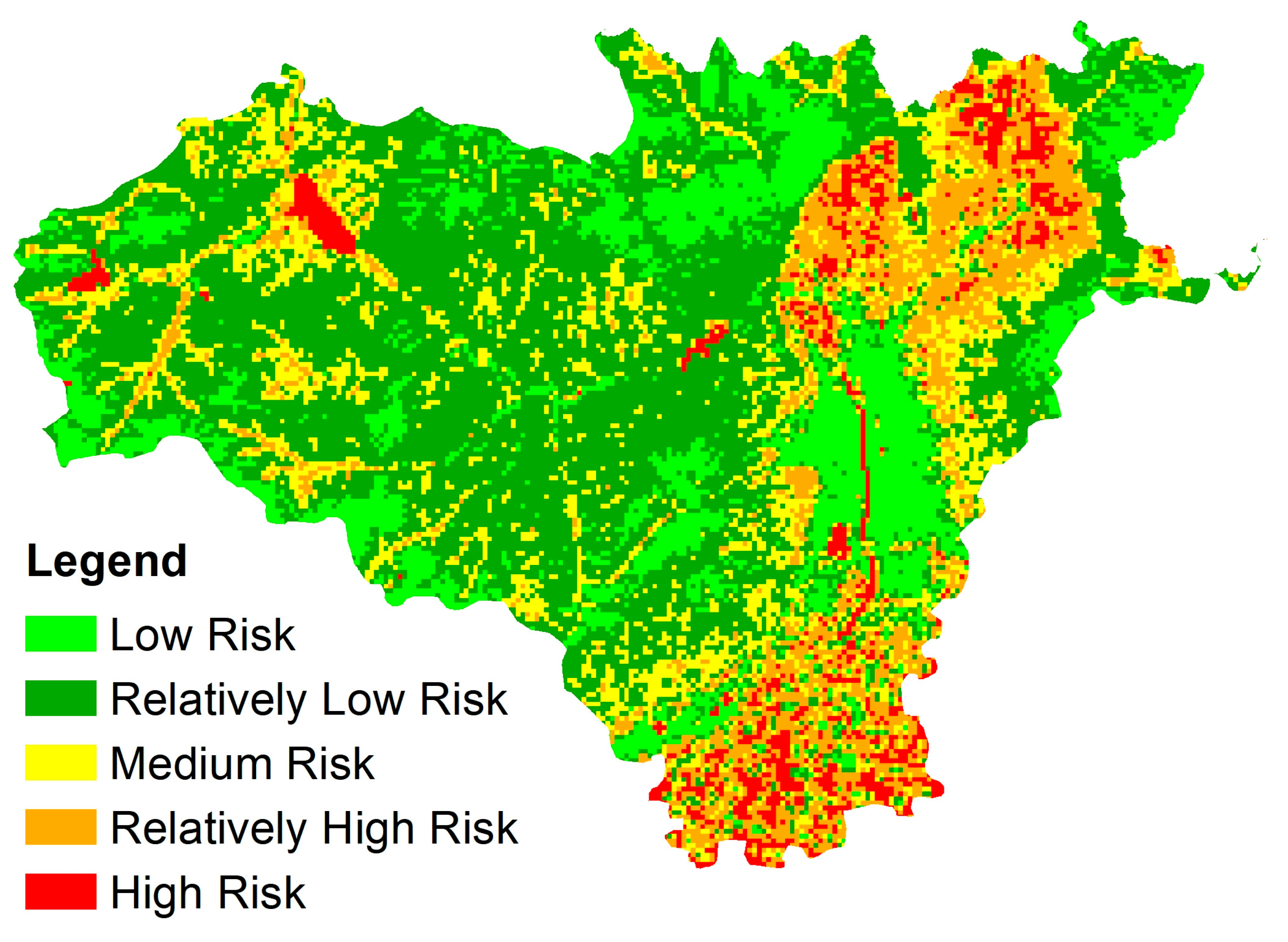
The results obtained at the 500 m, 700 m, and 900 m grid scales showed relatively consistent broad-scale spatial patterns, although the classification of local risk levels was affected by grid size. For example, in 2019, compared with the 500 m grid, the 900 m grid produced noticeable differences in the distribution of relatively high- and high-risk areas in the northeastern and southern parts of the study area. These differences may be attributable to the spatial clustering of risk factors, neighborhood aggregation effects, and classification-threshold effects. Therefore, the results demonstrate a certain degree of robustness in terms of the overall spatial pattern, but they are not entirely consistent with respect to local risk levels and the extent of high-risk areas. The 700 m grid was selected as a compromise between spatial detail and overall pattern stability. As a supplementary sensitivity experiment, the threshold for the 500 m grid in 2019 was reduced by 0.01 (Figure A4).
Figure A1.
Spatial distribution of landscape ecological risk at 500 m, 700 m, and 900 m grid scales: (a–c) 2014, (d–f) 2019, and (g–i) 2024.
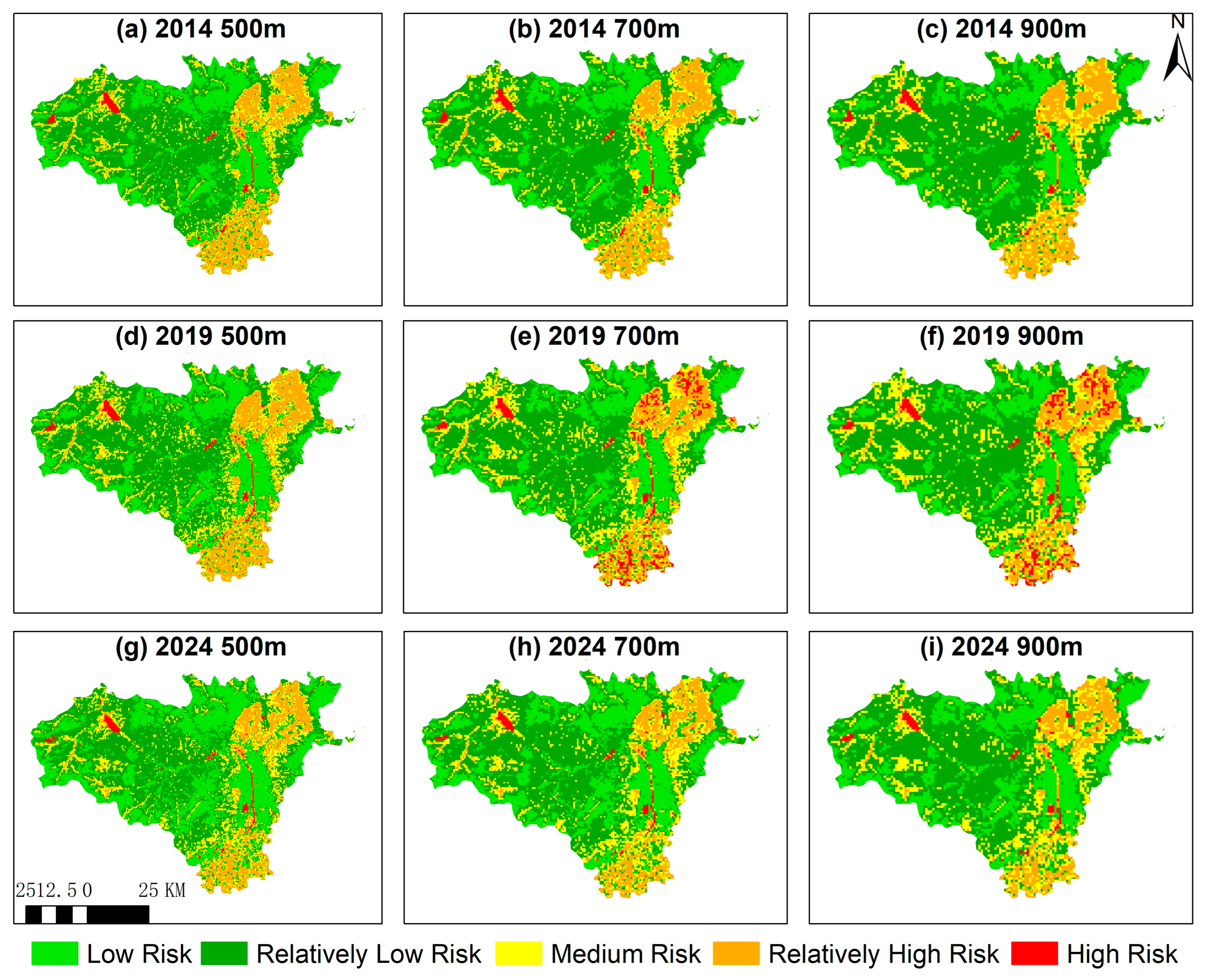
Figure A2.
Landscape ecological risk grade areas (km2) at 500 m, 700 m and 900 m grid scales.
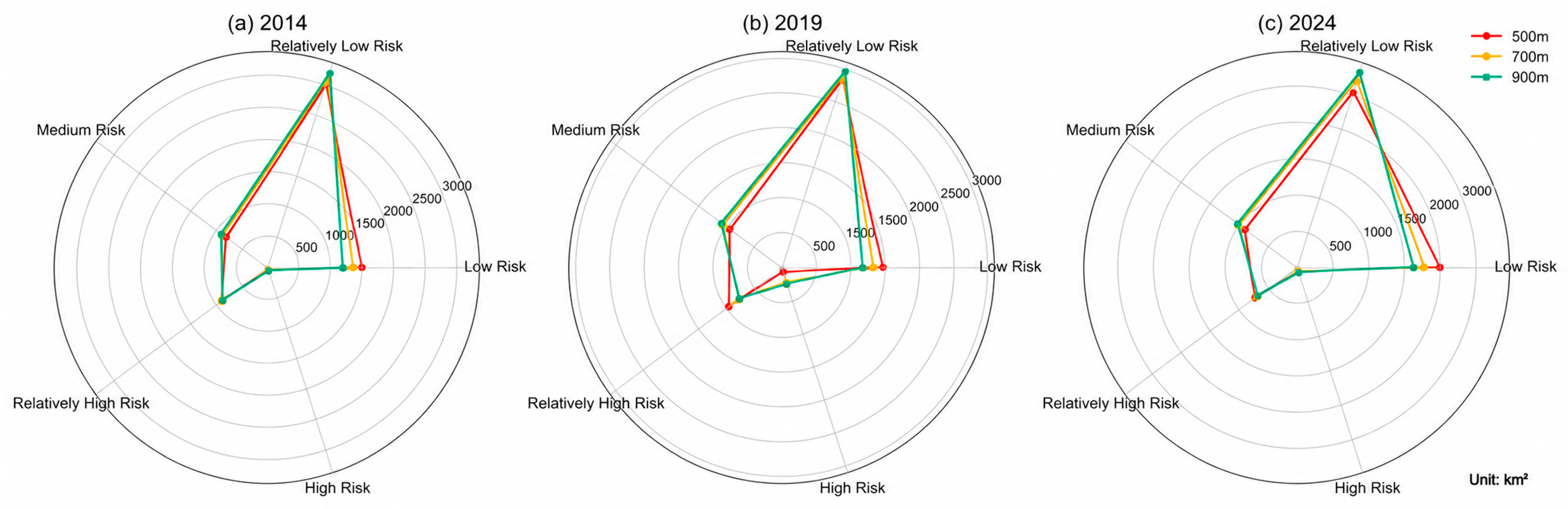
Figure A3.
Sensitivity Analysis of Landscape Ecological Risk Types Based on 500 m Grids in 2019.
Appendix A.2
A semivariogram analysis was conducted using the landscape ecological risk values to reassess the spatial blocking scale. The data exhibited a short-range spatial structure accounting for 73% of the total spatial variation and a secondary long-range spatial correlation structure accounting for the remaining 27%. Therefore, to improve the methodological rigor of the study, a spatial block side length of 15,400 m was used in the subsequent attribution analysis.
Figure A4.
Semivariogram model configuration and results for LER.
References
- Pickens, A.H.; Hansen, M.C.; Song, Z.; Poulson, A.; Komarova, A.; Baggett, A.; Kerr, T.; Mikus, A.; Dominguez, C.O.; Tyukavina, A.; et al. Rapid monitoring of global land change. Nat. Commun. 2025, 16, 8948. [Google Scholar] [CrossRef] [Scilit] [PubMed]
- Soni, H.; Yadav, R.K.; Patra, S.K. Global impact of urbanization on ecosystems: A comprehensive bibliometric analysis. Nat. Hazards Res. 2025, 5, 21–35. [Google Scholar] [CrossRef] [Scilit]
- Du, L.; Dong, C.; Kang, X.; Qian, X.; Gu, L. Spatiotemporal evolution of land cover changes and landscape ecological risk assessment in the Yellow River Basin, 2015–2020. J. Environ. Manag. 2023, 332, 117149. [Google Scholar] [CrossRef] [Scilit] [PubMed]
- Seto, K.C.; Güneralp, B.; Hutyra, L.R. Global forecasts of urban expansion to 2030 and direct impacts on biodiversity and carbon pools. Proc. Natl. Acad. Sci. USA 2012, 109, 16083–16088. [Google Scholar] [CrossRef] [Scilit] [PubMed]
- Cheng, X.; Zhang, Y.; Nie, W.; Wang, Y.; Wang, J.; Xu, B. Landscape ecological risk assessment and influencing factor analysis of basins in suburban areas of large cities—A case study of the Fuchunjiang River Basin, China. Front. Ecol. Evol. 2023, 11, 1184273. [Google Scholar] [CrossRef] [Scilit]
- Tonetti, V.; Pena, J.C.; Scarpelli, M.D.; Sugai, L.S.; Barros, F.M.; Anunciação, P.R.; Santos, P.M.; Tavares, A.L.; Ribeiro, M.C. Landscape heterogeneity: Concepts, quantification, challenges and future perspectives. Environ. Conserv. 2023, 50, 83–92. [Google Scholar] [CrossRef] [Scilit]
- Guo, H.; Cai, Y.; Li, B.; Wan, H.; Yang, Z. An improved approach for evaluating landscape ecological risks and exploring its coupling coordination with ecosystem services. J. Environ. Manag. 2023, 348, 119277. [Google Scholar] [CrossRef] [Scilit] [PubMed]
- Li, S.; Tu, B.; Zhang, Z.; Wang, L.; Zhang, Z.; Che, X.; Wang, Z. Exploring new methods for assessing landscape ecological risk in key basin. J. Clean. Prod. 2024, 461, 142633. [Google Scholar] [CrossRef] [Scilit]
- Zhang, Z.; Yu, H.; He, N.; Jin, G. Future land use simulation model-based landscape ecological risk prediction under the localized shared socioeconomic pathways in the Xiangjiang River Basin, China. Environ. Sci. Pollut. Res. 2024, 31, 22774–22789. [Google Scholar] [CrossRef] [Scilit] [PubMed]
- Deng, R.; Ding, X.; Wang, J. Landscape ecological risk assessment and spatial pattern evolution analysis of the Central Yunnan Urban Agglomeration from 1995 to 2020 based on land use/cover change. Sustainability 2023, 15, 16641. [Google Scholar] [CrossRef] [Scilit]
- Du, J.; Liu, B.; Jing, M.; Zhou, Y.; Yan, Q.; Li, G. Construction of ecological security pattern of arid area based on landscape ecological risk assessment: A case study of the Wu-Chang-Shi urban agglomeration. Environ. Sci. Pollut. Res. 2024, 31, 45622–45635. [Google Scholar] [CrossRef] [Scilit] [PubMed]
- Yang, N.; Zhang, T.; Li, J.; Feng, P.; Yang, N. Landscape ecological risk assessment and driving factors analysis based on optimal spatial scales in Luan River Basin, China. Ecol. Indic. 2024, 169, 112821. [Google Scholar] [CrossRef] [Scilit]
- Sui, X.; Sun, Y.; Wang, X.; Yuan, J. Research on ecological quality and restoration of fragile mining areas in the Yellow River Basin—The case of Xiegou coal mine. Ecol. Indic. 2025, 174, 113426. [Google Scholar] [CrossRef] [Scilit]
- Li, X.; Li, S.; Zhang, Y.; O’Connor, P.J.; Zhang, L.; Yan, J. Landscape ecological risk assessment under multiple indicators. Land 2021, 10, 739. [Google Scholar] [CrossRef] [Scilit]
- Lin, X.; Wang, Z. Landscape ecological risk assessment and its driving factors of multi-mountainous city. Ecol. Indic. 2023, 146, 109823. [Google Scholar] [CrossRef] [Scilit]
- Xue, L.; Zhu, B.; Wu, Y.; Wei, G.; Liao, S.; Yang, C.; Wang, J.; Zhang, H.; Ren, L.; Han, Q. Dynamic projection of ecological risk in the Manas River basin based on terrain gradients. Sci. Total Environ. 2019, 653, 283–293. [Google Scholar] [CrossRef] [Scilit] [PubMed]
- Mo, W.; Wang, Y.; Zhang, Y.; Zhuang, D. Impacts of road network expansion on landscape ecological risk in a megacity, China: A case study of Beijing. Sci. Total Environ. 2017, 574, 1000–1011. [Google Scholar] [CrossRef] [Scilit] [PubMed]
- Lin, Y.; Zhang, F.; Jin, Y.; Wen, L.; Yu, Y.; Zhang, L.; Weng, A.; Ge, Y. Spatial non-stationarity effects of the driving factors on landscape ecological risk: A case of the Xiamen-Zhangzhou-Quanzhou Urban Agglomeration, China. Ecol. Indic. 2024, 167, 112660. [Google Scholar] [CrossRef] [Scilit]
- Zhang, X.; Yu, J.; Feng, H.; Yao, L.; Li, X.; Du, H.; Liu, Y. Landscape ecological risk and drivers of land-use transition under the perspective of differences in topographic gradient. Land 2024, 13, 876. [Google Scholar] [CrossRef] [Scilit]
- Zhu, C.; Zhang, X.; Zhou, M.; He, S.; Gan, M.; Yang, L.; Wang, K. Impacts of urbanization and landscape pattern on habitat quality using OLS and GWR models in Hangzhou, China. Ecol. Indic. 2020, 117, 106654. [Google Scholar] [CrossRef] [Scilit]
- Chen, H.; Chen, H.; Huang, X.; Zhang, S.; He, T.; Gao, Z. Landscape ecological risk assessment and driving factor analysis in southwest China. Sci. Rep. 2024, 14, 23208. [Google Scholar] [CrossRef] [Scilit] [PubMed]
- Liu, L.; Wei, J.; Luo, P.; Zhang, Y.; Wang, Y.; Elbeltagi, A.; Zainol, M.R.R.M.A. A novel quantity assessment of landscape ecological risk using human-nature driving mechanism for sustainable society. Sci. Total Environ. 2024, 947, 173892. [Google Scholar] [CrossRef] [Scilit] [PubMed]
- Qiao, B.; Yang, H.; Cao, X.; Zhou, B.; Wang, N.A. Driving mechanisms and threshold identification of landscape ecological risk: A nonlinear perspective from the Qilian Mountains, China. Ecol. Indic. 2025, 173, 113342. [Google Scholar] [CrossRef] [Scilit]
- Zeng, J.; Wu, J.; Chen, W. Coupling analysis of land use change with landscape ecological risk in China: A multi-scenario simulation perspective. J. Clean. Prod. 2024, 435, 140518. [Google Scholar] [CrossRef] [Scilit]
- Li, M.; Abuduwaili, J.; Liu, W.; Feng, S.; Saparov, G.; Ma, L. Application of geographical detector and geographically weighted regression for assessing landscape ecological risk in the Irtysh River Basin, Central Asia. Ecol. Indic. 2024, 158, 111540. [Google Scholar] [CrossRef] [Scilit]
- Yu, T.; Bao, A.; Xu, W.; Guo, H.; Jiang, L.; Zheng, G.; Yuan, Y.; Nzabarinda, V. Exploring variability in landscape ecological risk and quantifying its driving factors in the Amu Darya Delta. Int. J. Environ. Res. Public Health 2020, 17, 79. [Google Scholar]
- Wang, W.; Xue, X.; Wang, Z.; Zhang, Q. Multiscale driving mechanisms and spatial non-stationarity of landscape ecological risk based on an OPGD–MGWR framework: Evidence from township-level units in the Nanjing metropolitan area (NMA), China. Ecol. Indic. 2026, 186, 114840. [Google Scholar] [CrossRef] [Scilit]
- Li, H.; Zhang, S.; Zeng, Y.; Xu, Z.; Yang, X.; Liu, Y. Multiscale landscape ecological risk response to natural and social factors in China: Thresholds identification. Habitat Int. 2026, 168, 103691. [Google Scholar] [CrossRef] [Scilit]
- Gao, J.; Pan, N.; Zhou, D. Integrating Landscape Ecological Risk and Ecosystem Services for Ecological Zoning in the Qilian Mountain National Park. Ecosyst. Health Sustain. 2025, 11, 0441. [Google Scholar] [CrossRef] [Scilit]
- Wu, Y.; Luo, M.; Ding, S.; Han, Q. Using a Light Gradient-Boosting Machine–Shapley Additive Explanations Model to Evaluate the Correlation Between Urban Blue–Green Space Landscape Spatial Patterns and Carbon Sequestration. Land 2024, 13, 1965. [Google Scholar] [CrossRef] [Scilit]
- He, N.; Ding, R. A dual-method approach integrating dynamic QCA and LightGBM-SHAP algorithms to uncover the configuration paths and key drivers of water resource green efficiency in China. Ecol. Indic. 2025, 175, 113540. [Google Scholar] [CrossRef] [Scilit]
- Liu, S.; Zhang, L.; Chi, Y.; Fu, L.; Wang, J.; Wang, X. Evaluating the Coupling Coordination Degree of the Water-Energy-Ecology System in the Yellow River Basin. Ecol. Indic. 2025, 182, 114461. [Google Scholar] [CrossRef] [Scilit]
- Wang, Y.; Wang, X.; Zhang, W.; Man, W.; Liu, M.; Jiao, L. Spatiotemporal evolution of landscape ecological risk and its driving factors of the Beijing–Tianjin–Hebei major mineral belt, 1985–2022. Sci. Rep. 2025, 15, 2425. [Google Scholar] [CrossRef] [Scilit] [PubMed]
- Du, J.; Bi, S.; Zhang, Y.; Chen, M. Landscape ecological risk assessment and driving factors in Guyi Basin cultural heritage sites: A multi-scenario simulation perspective. npj Herit. Sci. 2026, 14, 36. [Google Scholar] [CrossRef] [Scilit]
- Li, Z.; Ding, X.; Wang, S.; Wang, H.; Yan, Y.; Zhang, T.; Long, Y. Landscape Ecological Risk Assessment and Driving Factors During 1995–2024 in the Dianzhong Five Lakes Region of Yunnan Province, China Using the XGBoost-SHAP and Random Forest Models. Land 2026, 15, 508. [Google Scholar] [CrossRef] [Scilit]
- Zhang, S.; Feng, Z.; Kang, L.; Wu, K. Unraveling nonlinear landscape pattern effects on habitat quality: A Yangtze river delta case study for data-driven management. J. Environ. Manag. 2025, 394, 127665. [Google Scholar] [CrossRef] [Scilit] [PubMed]
- Wang, H.; Zhang, Y.A.; Niu, J.; Huang, W.; Yin, J.; Liu, D. Trade-offs between land use intensity and ecosystem services in ecologically critical areas from a decoupling perspective and their policy implications. Ecol. Indic. 2026, 182, 114505. [Google Scholar] [CrossRef] [Scilit]
- Qiao, Q.; Zhen, Z.; Liu, L.; Luo, P. The Construction of Ecological Security Pattern under Rapid Urbanization in the Loess Plateau: A Case Study of Taiyuan City. Remote Sens. 2023, 15, 1523. [Google Scholar] [CrossRef] [Scilit]
- Li, Q.; Ma, B.; Zhao, L.; Mao, Z.; Luo, L.; Liu, X. Landscape Ecological Risk Evaluation Study under Multi-Scale Grids—A Case Study of Bailong River Basin in Gansu Province, China. Water 2023, 15, 3777. [Google Scholar] [CrossRef] [Scilit]
- Xie, H.; Wang, P.; Huang, H. Ecological Risk Assessment of Land Use Change in the Poyang Lake Eco-economic Zone, China. Int. J. Environ. Res. Public Health 2013, 10, 328–346. [Google Scholar] [CrossRef] [Scilit] [PubMed]
- De Lange, H.J.; Sala, S.; Vighi, M.; Faber, J.H. Ecological vulnerability in risk assessment—A review and perspectives. Sci. Total Environ. 2010, 408, 3871–3879. [Google Scholar] [CrossRef] [Scilit] [PubMed]
- Guo, Y.; Guo, W. Landscape ecological risk analysis of urban agglomeration in the central basin of Shanxi from the perspective of “production-living-ecological spaces. Chin. J. Ecol. 2022, 41, 1813–1824. (In Chinese) [Google Scholar]
- Anselin, L. Spatial Econometrics: Methods and Models; Springer Science & Business Media: Berlin/Heidelberg, Germany, 1988. [Google Scholar]
- Anselin, L. Local indicators of spatial association—LISA. Geogr. Anal. 1995, 27, 93–115. [Google Scholar] [CrossRef] [Scilit]
- Ke, G.; Meng, Q.; Finley, T.; Wang, T.; Chen, W.; Ma, W.; Ye, Q.; Liu, T.-Y. LightGBM: A Highly Efficient Gradient Boosting Decision Tree. Adv. Neural Inf. Process. Syst. 2017, 30, 3146–3154. [Google Scholar]
- Cuomo, S.; Di Cola, V.S.; Giampaolo, F.; Rozza, G.; Raissi, M.; Piccialli, F. Scientific machine learning through physics–informed neural networks: Where we are and what’s next. J. Sci. Comput. 2022, 92, 88. [Google Scholar] [CrossRef] [Scilit]
- Friedman, J.H. Greedy function approximation: A gradient boosting machine. Ann. Stat. 2001, 29, 1189–1232. [Google Scholar] [CrossRef] [Scilit]
- Draper, N.R.; Smith, H. Applied Regression Analysis; John Wiley & Sons: Hoboken, NJ, USA, 1998. [Google Scholar]
- Lundberg, S.M.; Lee, S.I. A unified approach to interpreting model predictions. Adv. Neural Inf. Process. Syst. 2017, 30, 4768–4777. [Google Scholar]
- Gao, H.; Song, W. Assessing the Landscape Ecological Risks of Land-Use Change. Int. J. Environ. Res. Public Health 2022, 19, 13945. [Google Scholar] [CrossRef] [Scilit] [PubMed]
- Nafi’Shehab, Z.; Jamil, N.R.; Aris, A.Z.; Shafie, N.S. Spatial variation impact of landscape patterns and land use on water quality across an urbanized watershed in Bentong, Malaysia. Ecol. Indic. 2021, 122, 107254. [Google Scholar] [CrossRef] [Scilit]
- Chen, J.; Zhang, L.; Zhao, S.; Zong, H. Assessing Land-Use Conflict Potential and Its Correlation with LULC Based on the Perspective of Multi-Functionality and Landscape Complexity: The Case of Chengdu, China. Land 2023, 12, 742. [Google Scholar] [CrossRef] [Scilit]
- Gao, C.; Zhang, W.; Li, C.; Fan, Y. Landscape Ecological Risk Assessment and Analysis of Driving Factors in the Zhang–Wei River Basin, North China Plain. Sustainability 2026, 18, 2170. [Google Scholar] [CrossRef] [Scilit]
- Guo, B.; Xu, M.; Zhang, R.; Luo, W. A new monitoring index for ecological vulnerability and its application in the Yellow River Basin, China from 2000 to 2022. J. Arid Land 2024, 16, 1163–1182. [Google Scholar] [CrossRef] [Scilit]
- Karimian, H.; Zou, W.; Chen, Y.; Xia, J.; Wang, Z. Landscape ecological risk assessment and driving factor analysis in Dongjiang river watershed. Chemosphere 2022, 307, 135835. [Google Scholar] [CrossRef] [Scilit] [PubMed]

Disclaimer/Publisher’s Note: The statements, opinions and data contained in all publications are solely those of the individual author(s) and contributor(s) and not of MDPI and/or the editor(s). MDPI and/or the editor(s) disclaim responsibility for any injury to people or property resulting from any ideas, methods, instructions or products referred to in the content. |
© 2026 by the authors. Licensee MDPI, Basel, Switzerland. This article is an open access article distributed under the terms and conditions of the Creative Commons Attribution (CC BY) license.