Spatiotemporal Dynamics and Predictors of Cropland Change in Hunan Province, China: An XGBoost-SHAP Approach

Abstract

This study examines the spatiotemporal patterns of cropland change in Hunan Province and identifies the factors associated with net cropland decrease from 2000 to 2020. Using land-use transition analysis, spatial autocorrelation, Lorenz curves, Gini coefficients, and an interpretable XGBoost-SHAP model, this study analyzed cropland outflow, cropland inflow, net cropland change, and their associated explanatory patterns. The results show that: (1) cropland outflow was mainly concentrated in central and western Hunan, whereas cropland inflow was relatively more evident in central Hunan, but also occurred in parts of western and eastern Hunan. Total cropland area increased by 2961.73 km² from 2000 to 2020, but decreased by 1467.91 km² after peaking in 2009, indicating an inverted U-shaped trajectory; (2) the Gini coefficient of cropland outflow decreased from 0.4024 to 0.2891, while that of cropland inflow decreased from 0.3780 to 0.2538, indicating stronger spatial concentration of cropland outflow, although its spatial imbalance weakened over time; and (3) XGBoost-SHAP results showed that mechanical efficiency, gross domestic product (GDP), and fiscal conditions made the highest contributions to net cropland decrease, with mean absolute SHAP values of 0.21, 0.17, and 0.16, respectively. Overall, cropland change exhibited clear spatial heterogeneity, and socioeconomic and human-activity factors were dominant factors associated with net cropland decrease. These findings provide support for differentiated cropland protection and sustainable land-use management in major grain-producing regions.

1. Introduction

Hunan Province, as one of China’s major grain-producing regions, is located in areas characterized by a double-cropping system and an annual precipitation exceeding 1000 mm. The province ranks first nationally in both early rice planting area, covering approximately 12,109 km², and total rice production, amounting to 7.33 million tonnes [1,2]. While production has steadily increased, sediment accumulation and reclamation around Dongting Lake, the largest lake in Hunan Province, have caused its surface area to decrease by 47.93% between 1896 and 2014 [3]. Furthermore, concentrated cropland around Dongting Lake coexists with fragmented cropland in other regions of Hunan [4,5]. Recently, a phenomenon of rural “re-agriculturalization” has emerged, whereby young people return to agricultural activities, intersecting with ongoing urbanization trends [6,7,8]. Maintaining a stable cropland base is essential for safeguarding food security and supporting agricultural modernization [9,10]. In particular, the development of new quality productive forces in agriculture requires secure and well-organized agricultural production space [11,12]. Therefore, against the broader goal of stabilizing agricultural production capacity, investigating the spatiotemporal dynamics of cropland in Hunan Province is of substantial practical and comparative significance [13]. From a broader land-system perspective, cropland change reflects coupled interactions among food-security demands, socioeconomic development, institutional arrangements, and biophysical conditions across multiple scales [14,15]. More broadly, Hunan represents a typical traditional agricultural region in which food-security requirements, urbanization pressure, agricultural modernization, rural livelihood transformation, and land conversion under structural change intersect. Its cropland dynamics therefore provide a useful empirical window for understanding land-use transition processes in other major grain-producing regions facing similar tensions between cropland protection and development demand.

To date, studies on cropland change have approached the topic from different perspectives. A common focus is the analysis of land-use transitions between different land types rather than merely net increases or decreases [16,17,18]. For instance, Liu et al. [19] reported that between 2010 and 2015, cropland area decreased in southern China and increased in northern China, with the total area remaining stable; the center of newly added cropland shifted from the northeast to the northwest. Differences among studies are mainly reflected in three dimensions: spatial delineation, methodological approach, and causal analysis.

In terms of spatial delineation, researchers typically define cropland change in terms of non-agriculturalization and non-grain utilization, selecting datasets accordingly to represent cropland variation within the study area. Generally, non-agricultural use refers to cropland employed for activities other than agricultural production, while non-grain use refers to cropland utilized for purposes other than grain production [20,21,22]. Methodologically, studies adopt various technical approaches and inferential models (as detailed in Table 1), including Geographical Detector analysis [23], empirical analysis [24], remote sensing interpretation [25], and boosted regression tree (BRT) algorithms [26]. In causal analyses, previous studies have commonly used socioeconomic indicators from statistical yearbooks, together with multisource spatial data such as distance, density, survey, and remote-sensing variables, to identify the drivers of cropland change [27,28,29,30].

Table 1. Analysis of Cropland Change across Different Regions of China.

Research Area	Research Methods	Influencing Factors
Northeastern China	Geographic detector	Regional population size, urban–rural income gap, GDP, and the added value of the secondary and tertiary industries are the main influencing factors
Northwestern China	Empirical analysis	The expansion of production scale for relatively profitable agricultural products, advances in agricultural science and technology, and agriculture-related policies are the main influencing factors
Qinghai–Tibet Region, China	Remote sensing interpretation	Cropland protection policies, ecological conversion of farmland to forest/grassland, land development and consolidation projects, major construction projects, population, and urbanization processes are the main influencing factors
Southern China	BRT algorithm	Coastlines, water bodies, road traffic, distance to built-up areas, population, and per capita GDP are the main influencing factors

However, several limitations remain in existing studies. First, many studies have focused primarily on cropland loss, cropland outflow, or cropland non-agriculturalization, whereas the spatial patterns and driving mechanisms of cropland inflow have received comparatively less attention. Second, existing analyses often rely on single-source or single-dimensional datasets, which may limit a comprehensive understanding of cropland change. Third, although machine learning methods have increasingly been applied to land-use and cropland change studies [31,32,33,34], their ability to integrate multi-source variables and reveal nonlinear, threshold, and interaction effects remains insufficiently explored in analyses of net cropland decrease. And existing studies often emphasize prediction or factor ranking, while the nonlinear responses, threshold effects, and interactions associated with net cropland decrease remain insufficiently examined. SHAP improves model interpretability by quantifying variable contributions and revealing heterogeneous effects, but its explanations mainly indicate predictive associations rather than causal relationships, especially when explanatory variables are interdependent [35,36,37]. Therefore, an XGBoost-SHAP framework is employed to identify the key variables, non-linear patterns, and interaction effects associated with net cropland decrease, while improving model transparency and avoiding causal overinterpretation.

This study focuses on Hunan Province and adopts a multi-dimensional, multi-temporal, and multi-factorial approach to investigate cropland dynamics and associated factors. Utilizing natural, economic, and social datasets, the study employs spatial autocorrelation analysis, centroid migration modeling, Lorenz curves, Gini coefficients, and the XGBoost-SHAP model, implemented through ArcGIS 10.8 (ESRI, Redlands, CA, USA) and R software (version 4.4.1, R Core Team, Vienna, Austria). This study aims to identify the spatial patterns of cropland outflow, cropland inflow, and net cropland change from 2000 to 2020, examine the factors associated with net cropland decrease, and provide scientific support for cropland protection and sustainable land-use management in Hunan Province.

2. Materials and Methods

2.1. Study Area

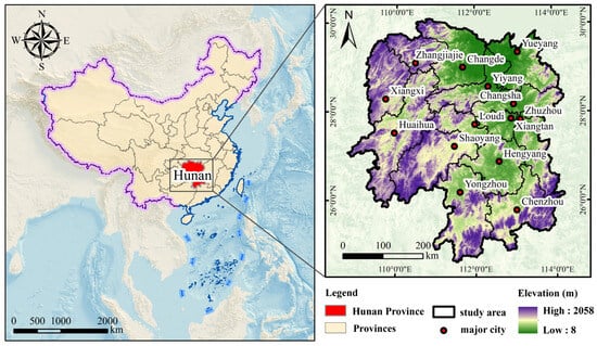
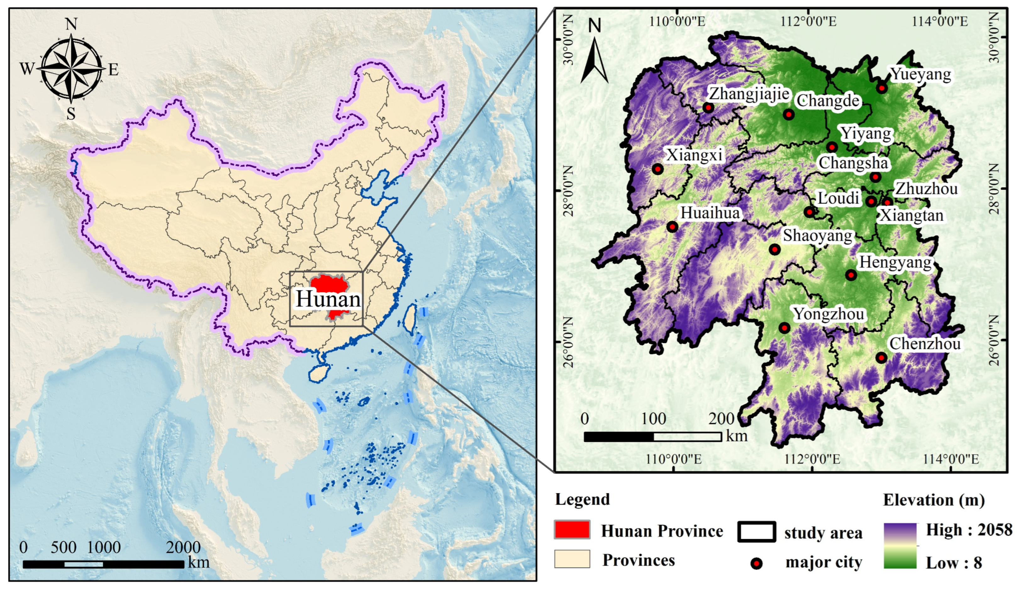
Hunan Province is located in central China, in the middle reaches of the Yangtze River, between 24°38′–30°08′ N and 108°47′–114°15′ E, with a total area of 211,800 km². In terms of natural conditions, Hunan lies in the transitional zone from the Yunnan–Guizhou Plateau to the Jiangnan Hills and from the Nanling Mountains to the Jianghan Plain (Figure 1). It is bordered by mountains to the east, south, and west, while the northern lake-basin plain opens toward the Yangtze River. Most of central Hunan consists of basins, hills, and terraces, with an average elevation below 500 m. Economically, Hunan’s gross regional product reached RMB 5.00129 trillion in 2023, and its gross agricultural output value reached RMB 819.94 billion. From 2013 to 2023, the gross value of agricultural production increased by RMB 152.2 billion. The province ranked among the leading regions in China in terms of agricultural socialized services, total agricultural machinery capacity, and moderate-scale farmland management under diverse operational forms.

Figure 1. The study area.

2.2. Data Sources and Processing

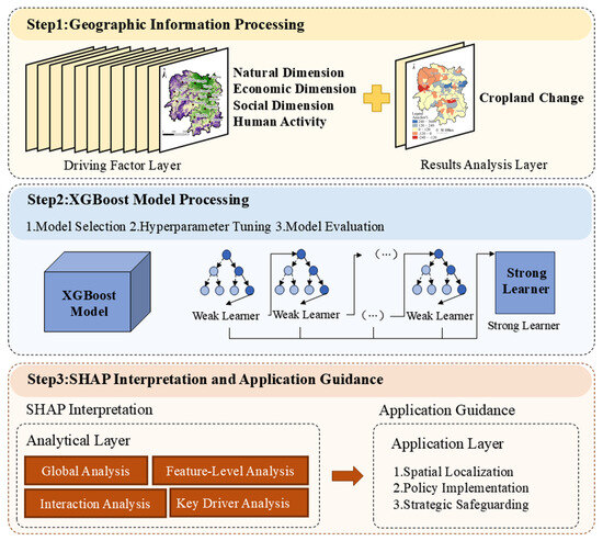
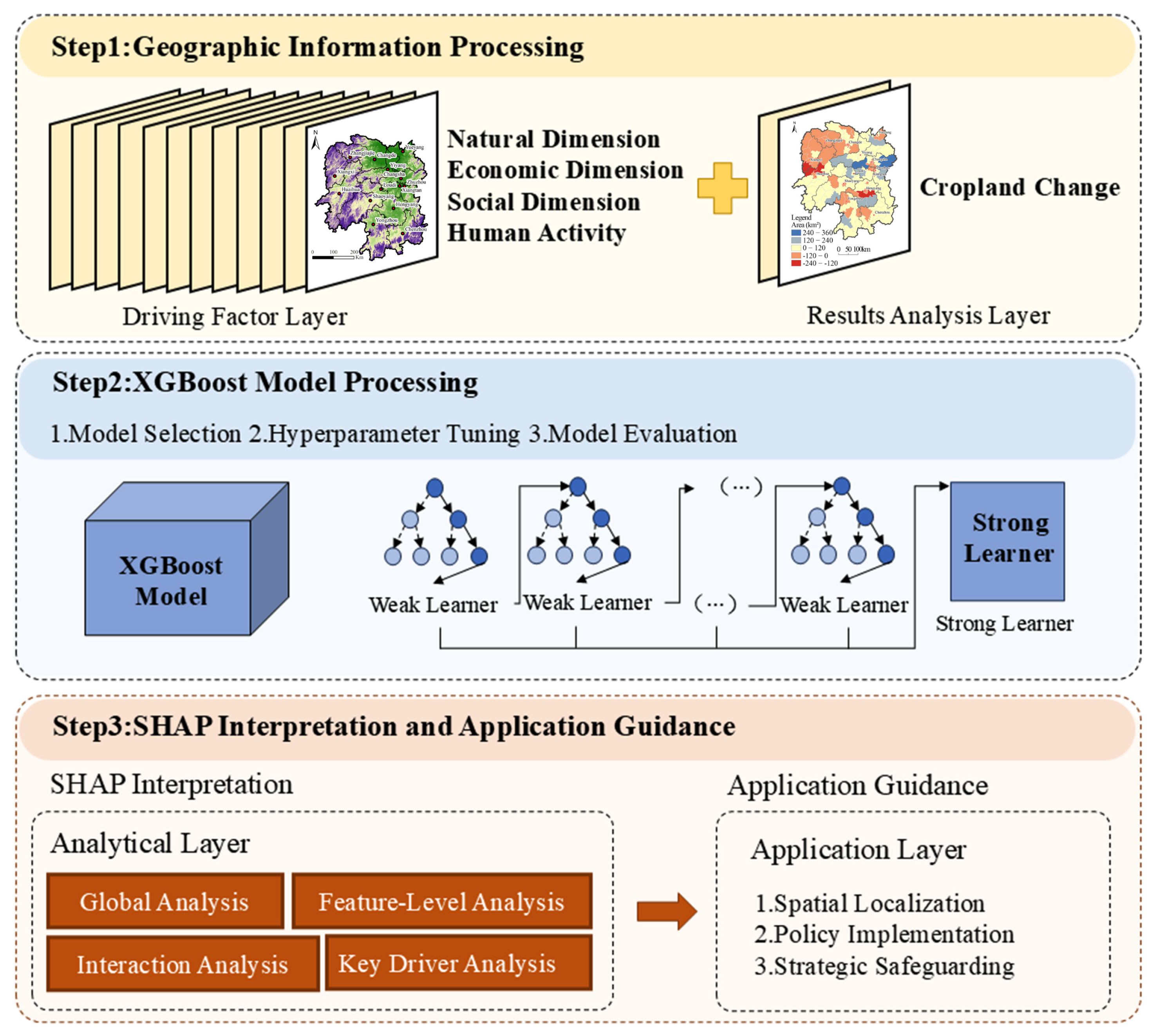
This study (Figure 2) used land-use data from 2000 to 2020 with a spatial resolution of 30 m × 30 m. The cropland data were obtained from the Landsat-derived China Land Cover Dataset (CLCD) published by Jie Yang and Xin Huang on the Google Earth Engine platform [38]. The CLCD dataset provides annual land-cover classification data for China and includes nine land-cover types: cropland, forest, shrub, grassland, water, snow/ice, barren land, impervious surface, and wetland. Based on this classification system, the cropland class was extracted as the basic land-use category for analyzing cropland transitions in Hunan Province. Natural-environment data were obtained from the Geospatial Data Cloud and the Resource and Environmental Science Data Center of the Chinese Academy of Sciences, while socioeconomic data were derived from the China County Statistical Yearbook and the Hunan Statistical Yearbook, as detailed in Table 2.

Figure 2. The framework of the research.

Table 2. Basic data.

Data Type	Data Name	Spatial Resolution	Data Source
Land data	Land data	30 m	China Annual Land Cover Dataset
Natural data	Elevation	30 m	Geospatial Data Cloud (http://www.gscloud.cn/home)
	Slope	30 m	Extracted from elevation data
	Soil data	1000 m	Resource and Environmental Science Data Center, Chinese Academy of Sciences (http://www.resdc.cn/)
Economic data	Regional GDP	1000 m	Resource and Environmental Science Data Center, Chinese Academy of Sciences (http://www.resdc.cn/)
	Fiscal revenue	1000 m	Hunan Statistical Yearbook; county-level statistical yearbooks, with missing years supplemented by interpolation
	Fiscal expenditure	1000 m	Hunan Statistical Yearbook; county-level statistical yearbooks, with missing years supplemented by interpolation
	Rural residents’ income	1000 m	Hunan Statistical Yearbook; county-level statistical yearbooks, with missing years supplemented by interpolation
Social data	Population density	1000 m	Resource and Environmental Science Data Center, Chinese Academy of Sciences (http://www.resdc.cn/)
	Urbanization rate	1000 m	Hunan Statistical Yearbook; county-level statistical yearbooks, with missing years supplemented by interpolation
	Rural labor force	1000 m	China County Statistical Yearbook; Hunan Statistical Yearbook, with missing years supplemented by interpolation
Human activity	Mechanical efficiency	1000 m	China County Statistical Yearbook; Hunan Statistical Yearbook, with missing years supplemented by interpolation
	Road density	1000 m	Resource and Environmental Science Data Center, Chinese Academy of Sciences (http://www.resdc.cn/)
	Nighttime light data	1000 m	Resource and Environmental Science Data Center, Chinese Academy of Sciences (http://www.resdc.cn/)
Vector data	Administrative boundary	County level	the standard base map from the Hunan Provincial Standard Map Service website (http://bzdt.ch.mnr.gov.cn/)

2.3. Methodology

2.3.1. Extraction of Cropland Outflow and Inflow

To identify cropland transitions during the study period, annual land-use raster data were overlaid in ArcGIS 10.8. Cropland outflow and cropland inflow were extracted by comparing the land-use types between two consecutive years. Cropland outflow refers to areas that were classified as cropland in year t − 1 but converted to non-cropland in year t, whereas cropland inflow refers to areas that were classified as non-cropland in year t − 1 but converted to cropland in year t.

In this study, cropland outflow and cropland inflow were calculated annually from 2000 to 2020 and were further summarized at the county level to analyze their spatial distribution characteristics and influencing factors.

2.3.2. Moran’s I

Global Moran’s I and Local Moran’s I were used to examine the spatial autocorrelation of cropland outflow and cropland inflow at five-year intervals from 2000 to 2020. Global Moran’s I measured overall spatial clustering, while Local Moran’s I identified local clusters and spatial outliers. Getis–Ord Gi* analysis was further applied to detect significant hotspot and coldspot areas. Moran’s I ranges from −1 to 1, with positive values indicating spatial clustering, values close to 0 indicating randomness, and negative values indicating spatial dispersion [39,40,41]. The formulas are presented in Equations (1) and (2).

$$Global Moran’s I={\displaystyle \frac{n{\sum }_{i=1}^n{\sum }_{j=1}^n{W}_{ij}(x_i-\overline{x})(x_j-\overline{x})}{\left({\sum }_{i=1}^n{\sum }_{j=1}^n{W}_{ij}\right){\sum }_{i=1}^n{(x_i-\overline{x})}^2}}$$

(1)

$$Local Moran’s I={\displaystyle \frac{n(x_i-\overline{x}){\sum }_{j=1}^n{W}_{ij}(x_i-\overline{x})}{{\sum }_{i=1}^n{(x_i-\overline{x})}^2}}$$

(2)

where $n$ denotes the number of samples; $x_i$ and $x_j$ represent the observed values of variable $x$ at spatial locations $i$ and $j$, respectively; $\overline{x}$ is the mean value of $x$; and $W_{ij}$ denotes the spatial weight. An adjacent spatial weight matrix was used in this study. If region $i$ and region $j$ are adjacent, $W_{ij}$ is assigned a value of 1; otherwise, it is assigned a value of 0.

2.3.3. Standard Deviational Ellipse

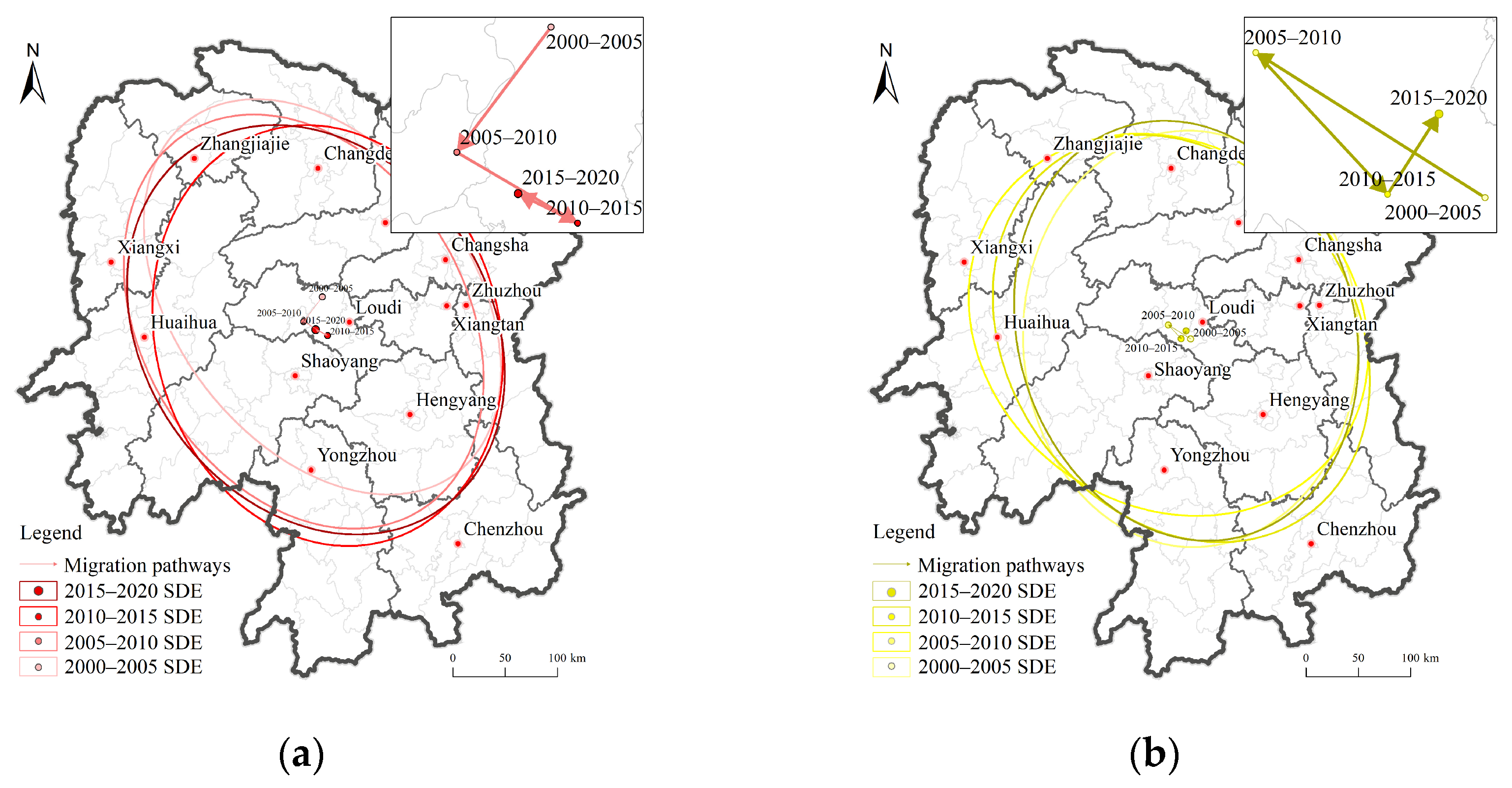
The standard deviational ellipse (SDE) is a widely used spatial statistical method for summarizing the central tendency, dispersion, and directional orientation of geographic features [42,43]. It characterizes spatial distribution through the mean center, major and minor axes, ellipse area, and rotation angle. In this study, SDE analysis was applied to identify the centroid migration and directional evolution of cropland outflow and cropland inflow across different time intervals from 2000 to 2020. Within each interval, the SDE was used to quantify the overall spatial concentration and orientation of cropland change from a province-wide perspective. The formula is presented in Equation (3).

$$C=\left[{\displaystyle \genfrac{}{}{0pt}{}{cov(x,y)}{cov(y,x)}}{\displaystyle \genfrac{}{}{0pt}{}{var\left(x\right)}{var\left(y\right)}}\right]={\displaystyle \frac{1}{n}}\left({\displaystyle \genfrac{}{}{0pt}{}{{\displaystyle {\sum }_{i=1}^n}{\overline{x_i}}^2}{{\displaystyle {\sum }_{i=1}^n}\overline{x_i}\overline{y_i}}}{\displaystyle \genfrac{}{}{0pt}{}{{\displaystyle {\sum }_{i=1}^n}\overline{x_i}\overline{y_i}}{{\displaystyle {\sum }_{i=1}^n}{\overline{y_i}}^2}}\right)$$

(3)

where $(x,y)$ denotes the longitude and latitude coordinates of each geographic feature, and $x$ and $y$ represent the coordinate deviations of each geographic feature from the mean center in the longitudinal and latitudinal directions, respectively.

2.3.4. Lorenz Curve and Gini Coefficient

The Lorenz curve and Gini coefficient have been widely used to quantify inequality, spatial concentration, and distributional imbalance in land-use studies [44,45]. In this study, the research period was divided into four intervals: 2000–2005, 2005–2010, 2010–2015, and 2015–2020. The Lorenz curve and Gini coefficient were used to evaluate the spatial concentration and imbalance of cropland outflow and cropland inflow in Hunan Province. The formula is presented in Equation (4).

$$Gini=1-{\sum }_{i=1}^n(x_{i+1}-x_i)(y_{i+1}+y_i)$$

(4)

where $Gini$ denotes the Gini coefficient of the spatial distribution of cropland outflow or cropland inflow; $n$ represents the number of counties in Hunan Province; $x_i$ denotes the cumulative proportion of cropland outflow or cropland inflow; and $y_i$ denotes the proportion of the land area of each county.

2.3.5. XGBoost-SHAP Method

The XGBoost algorithm is an ensemble learning method. It constructs multiple weak learners through residual fitting and integrates them into a strong learner. Each newly generated learner is trained based on the previously fitted model, thereby continuously optimizing model performance and enabling the final predictions to approximate the observed values as closely as possible [46,47]. However, XGBoost has limited interpretability and is often regarded as a black-box model, making it difficult to determine the relationships between selected features and prediction outcomes [48]. To address this limitation, researchers have introduced SHAP to enhance model interpretability [49].

The SHAP framework proposed by Lundberg uses Shapley values from game theory as an explanatory metric, thereby improving the interpretability of black-box models. Subsequent studies have demonstrated its advantages in terms of strong variable interpretability, quantification of variable contributions, and effective graphical visualization. Therefore, this study introduced the XGBoost-SHAP method to analyze the factors influencing cropland change in Hunan Province within the study area. This approach is highly applicable and enables interpretable analysis. The specific formulas are presented in Equations (5) and (6).

$$\widehat{y}={\displaystyle \sum _{k=1}^K}{f}_k(x_i)$$

(5)

$$L={\displaystyle {\sum }_{i=1}^m}l(y_i,{\widehat{y}}_i)+{\displaystyle {\sum }_{k=1}^K}\Omega (f_k)$$

(6)

where $x_i$ denotes the input variable; ${\widehat{y}}_i$ represents the predicted value generated by the prediction model for $x_i$; K denotes the number of regression trees; $f_k$ is the $k$th base learner; $L$ represents the loss function; and $\Omega$ denotes the regularization term.

3. Results

3.1. Current Spatial Pattern of Cropland in Hunan Province

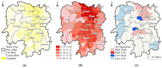
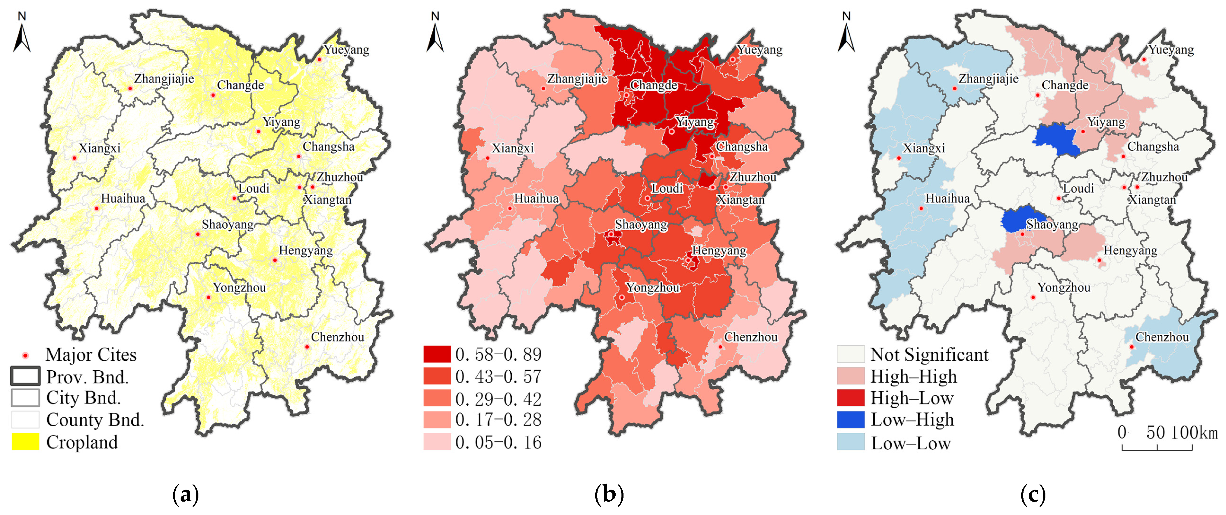
Based on the land-use dataset, cropland patches in Hunan Province were extracted according to the cropland classification code and converted into vector polygons (Figure 3a). To characterize county-level cropland distribution, this study introduced the indicator of cropland abundance, defined as the proportion of cropland area within each county. The cropland abundance values were classified into five levels using the Natural Breaks (Jenks) method in ArcGIS, thereby visualizing spatial variation in cropland proportions across the province (Figure 3b). Cluster and outlier analysis was then performed to identify local spatial association patterns of cropland distribution (Figure 3c). Figure 3c shows that High–High clusters were mainly distributed in northern and central Hunan, indicating counties with high cropland abundance surrounded by neighboring counties with similarly high cropland abundance. Low–Low clusters were primarily located in western and southern Hunan, reflecting contiguous areas with relatively low cropland abundance.

Figure 3. Spatial Distribution Pattern of Cropland in Hunan Province in 2023: (a) Distribution of Cropland; (b) Cropland Abundance; and (c) Cluster and Outlier Analysis of Cropland Distribution.

The results show that cropland resources are mainly concentrated in northern and central Hunan, whereas cropland is relatively sparse in western and southern Hunan, where topographic constraints are more pronounced. The Global Moran’s I value was 0.535, with a z-score of 8.247 and p < 0.001, indicating significant positive spatial autocorrelation and confirming that cropland distribution in Hunan Province exhibits a non-random clustered pattern.

3.2. Spatiotemporal Patterns of Cropland Change in Hunan Province

To characterize the spatiotemporal dynamics of cropland change, annual areas and spatial distributions of cropland outflow and cropland inflow were calculated, followed by a phased analysis of their spatiotemporal evolution. Polygon vectorization was performed without geometric simplification to preserve the spatial fidelity of cropland patches. The analysis consisted of two parts: (i) a disaggregated analysis of cropland outflow and cropland inflow from 2000 to 2020 (Section 3.2.1), and (ii) an integrated assessment of province-wide cropland change (Section 3.2.2).

3.2.1. Disaggregated Analysis

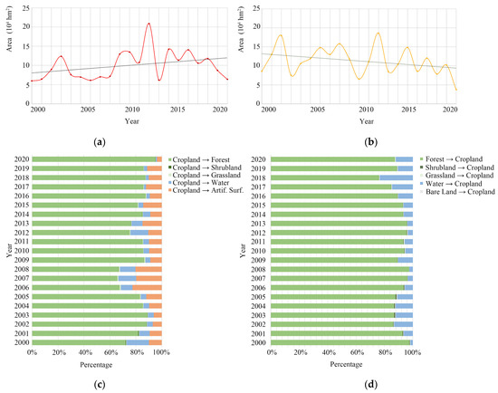
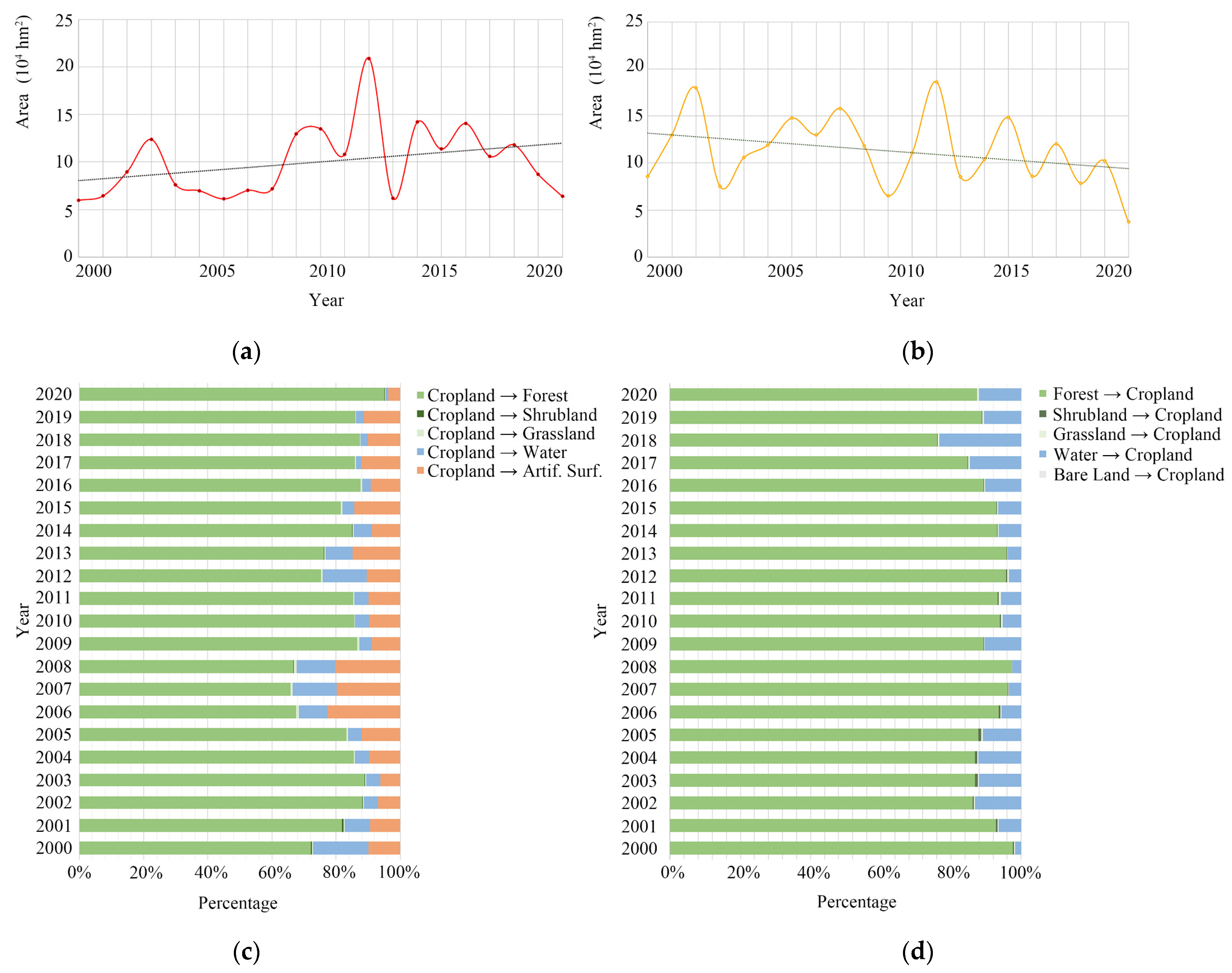
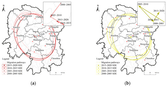
Cropland outflow exhibited a fluctuating temporal pattern during the study period, while the linear regression trendline indicated an overall upward tendency (Figure 4a). The maximum annual cropland outflow occurred in 2012, reaching 209,156.9 ha. In terms of land-cover transition types, cropland was mainly converted to forestland, artificial surfaces, and water bodies, whereas conversions to shrubland and grassland accounted for relatively small proportions (Figure 4c). Across successive intervals, the cumulative spatial extent of cropland outflow expanded gradually (Figure 5a). The SDE results showed that the centroid of areas of cropland outflow progressively migrated from the northwest toward the southeast (Figure 5a).

Figure 4. Spatiotemporal Trends and Transition-Type Analysis of Cropland Outflow and Inflow: (a) Trend of Cropland Outflow; (b) Trend of Cropland Inflow; (c) Land-Use Type Statistics of Cropland Outflow; (d) Land-Use Type Statistics of Cropland Inflow.

Figure 5. Standard Deviational Ellipse: (a) Cropland Outflow; (b) Cropland Inflow.

Cropland inflow also showed a fluctuating temporal pattern, but its linear regression trendline indicated an overall downward tendency (Figure 4b). The highest annual cropland inflow was also recorded in 2012, amounting to 186,185.4 ha. The main sources of cropland inflow were forestland, water bodies, and shrubland, while grassland and bare land contributed only marginally (Figure 4d). Across successive intervals, the cumulative spatial extent of areas converted to cropland declined (Figure 5b). The SDE centroid of areas of cropland inflow migrated in the opposite direction, shifting from the southeast toward the northwest (Figure 5b).

Global Moran’s I analysis showed that both cropland outflow and cropland inflow exhibited statistically significant positive spatial autocorrelation across all four subperiods: 2000–2005, 2005–2010, 2010–2015, and 2015–2020 (Table 3). For both processes, the z-scores exceeded 2.0 and the p-values were below 0.05, indicating that the spatial distributions of cropland outflow and cropland inflow were significantly clustered rather than randomly distributed. However, the relative strength of spatial clustering differed between the two processes and varied across periods. During 2000–2005, cropland inflow showed stronger spatial clustering than cropland outflow, as reflected by its higher Global Moran’s I and z-score. In contrast, from 2005 onward, cropland outflow consistently exhibited higher Global Moran’s I values and z-scores than cropland inflow, suggesting stronger spatial clustering of cropland loss in the later stages of the study period. Temporally, the spatial clustering of cropland outflow followed a non-monotonic pattern, increasing sharply from 2000–2005 to 2005–2010, declining during 2010–2015, and then increasing again during 2015–2020.

Table 3. Global Moran’s I of Cropland Change in Hunan Province.

Year	Spatial Distribution of Cropland Outflow			Spatial Distribution of Cropland Inflow
	G Morans’I	Z Value	p Value	G Morans’I	Z Value	p Value
2000~2005	0.284422	4.481715	<0.001	0.683081	10.623497	<0.001
2005~2010	0.746113	11.692810	<0.001	0.476428	7.399441	<0.001
2010~2015	0.526567	8.139247	<0.001	0.156024	2.564536	0.010
2015~2020	0.618520	9.514378	<0.001	0.268900	4.482475	<0.001

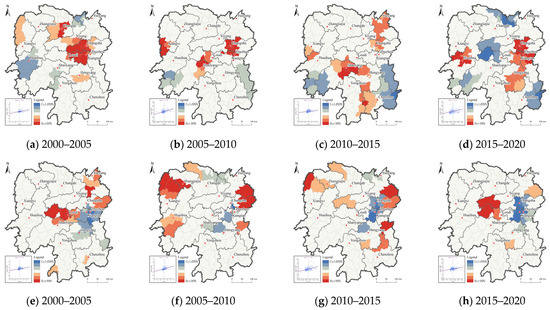
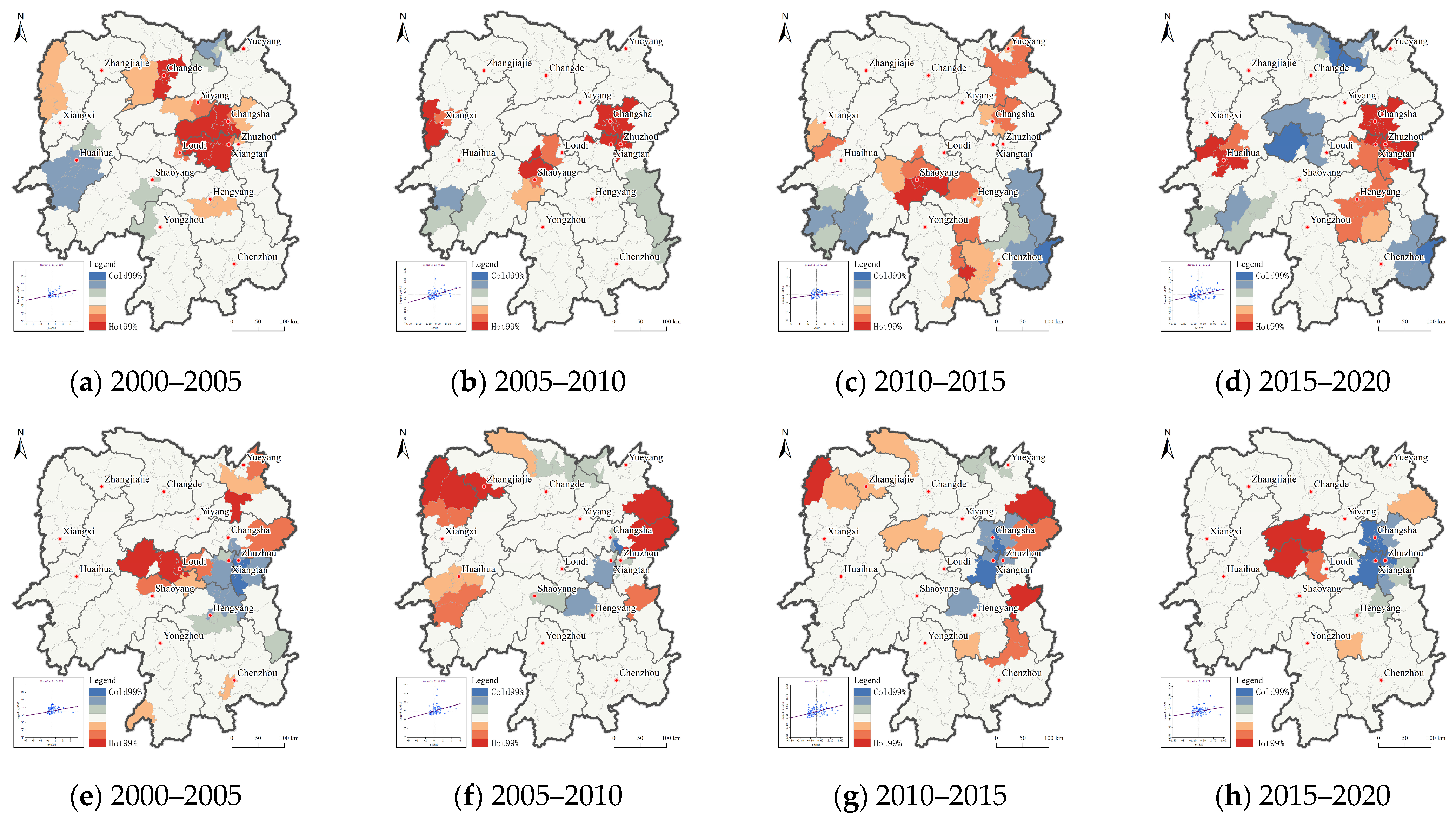
Local spatial association and hotspot–coldspot analyses were conducted to further examine the spatial clustering patterns of cropland outflow and cropland inflow in Hunan Province (Figure 6). The results show that both processes exhibited evident local spatial clustering across the four subperiods.

Figure 6. Local Moran’s I and Hotspot–Coldspot Analysis: (a–d) cropland outflow; (e–h) cropland inflow.

Hotspot–coldspot analysis showed clear spatial heterogeneity in cropland outflow and cropland inflow across Hunan Province. For cropland outflow, hotspots were mainly distributed in central and northern Hunan, while coldspots were more common in western and southern Hunan. In particular, outflow hotspots and inflow coldspots were repeatedly observed in Changsha and its surrounding urban agglomeration, where rapid urbanization, intensive construction activities, and mature secondary and tertiary industries may increase pressure for the conversion from cropland to non-cropland while limiting the potential for new cropland development. In addition to the Changsha metropolitan area, cropland outflow hotspots were also identified in western Hunan and parts of central Hunan, suggesting that cropland loss also occurred in areas with complex terrain and relatively constrained agricultural production conditions. By contrast, cropland inflow hotspots were more scattered and appeared mainly in parts of central, western, and eastern Hunan across different subperiods, with central Hunan showing relatively stronger inflow potential. Overall, the hotspot–coldspot patterns indicate that cropland change in Hunan Province was spatially heterogeneous and locally clustered, consistent with the significant positive Global Moran’s I results in Table 3.

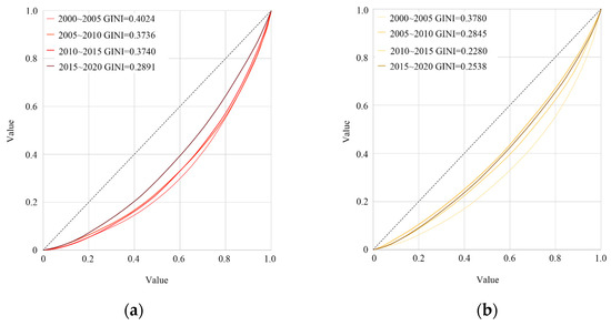
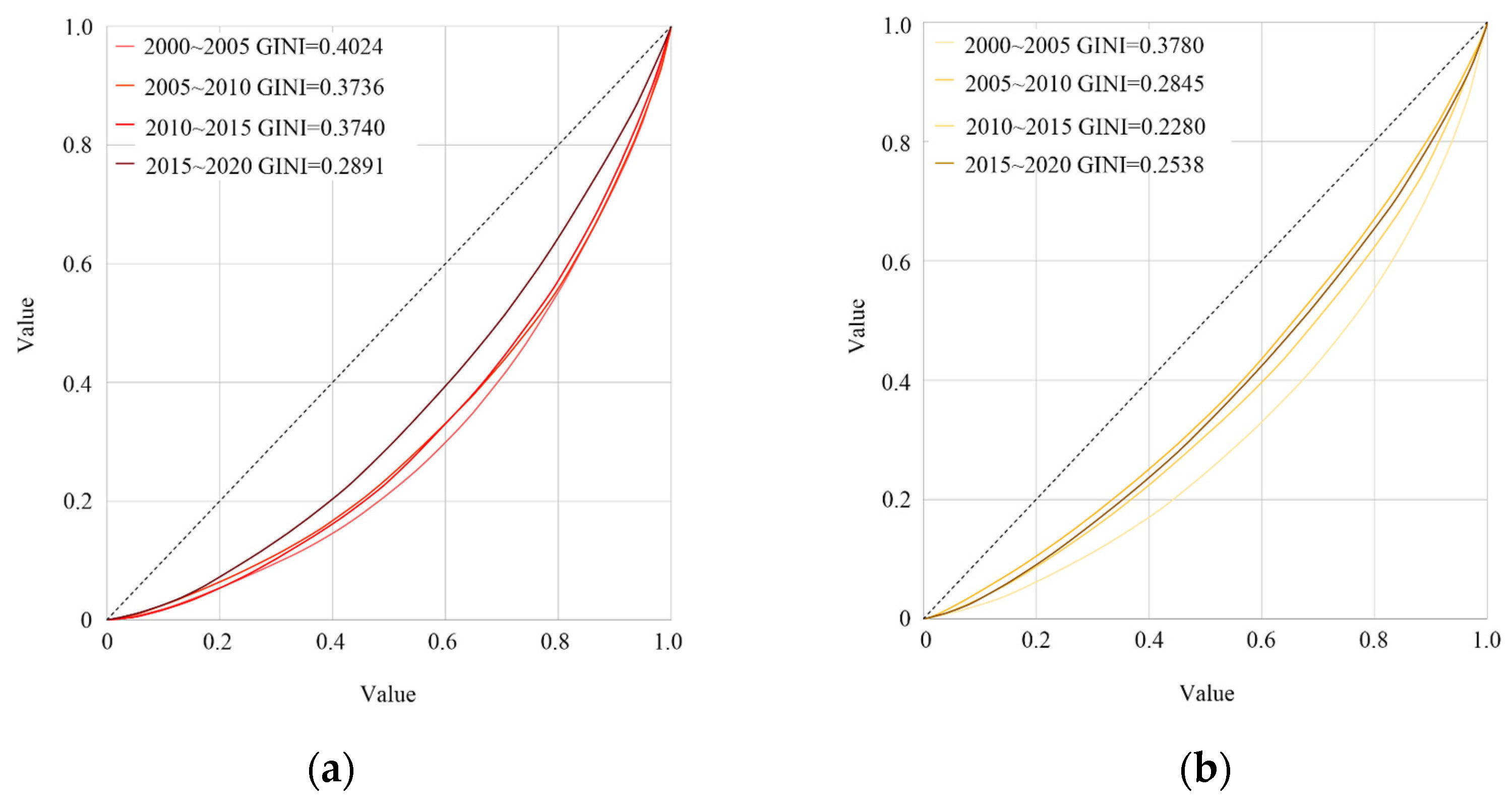
Using five-year intervals as the analytical units, Lorenz curves and Gini coefficients were calculated to evaluate the spatial concentration of areas of cropland outflow and areas of cropland inflow in Hunan Province. The Gini coefficients for areas of cropland outflow were 0.4024, 0.3736, 0.3740, and 0.2891 for 2000–2005, 2005–2010, 2010–2015, and 2015–2020, respectively. The corresponding values for areas of cropland inflow were 0.3780, 0.2845, 0.2280, and 0.2538. In all four periods, the Gini coefficients for areas of cropland outflow were higher than those for areas of cropland inflow, indicating that cropland outflow was more spatially concentrated than cropland inflow (Figure 7). Over time, the Lorenz curves for cropland outflow gradually approached the line of perfect equality, suggesting a decline in the spatial imbalance of cropland outflow. By contrast, the spatial imbalance of cropland inflow decreased during the first three periods but showed a slight rebound during 2015–2020.

Figure 7. The Gini Coefficient and Lorenz Curve: (a) cropland outflow; (b) cropland inflow.

3.2.2. Integrated Analysis

At the provincial scale, the total cropland area in Hunan Province showed an inverted U-shaped trajectory from 2000 to 2020, increasing initially and then decreasing, with a peak in 2009. Based on the endpoint comparison between 2000 and 2020, the province recorded a net cropland increase of 2961.73 km² over the entire study period. However, after the 2009 peak, cropland area declined by 1467.91 km² between 2009 and 2020, indicating a shift from net expansion to net contraction.

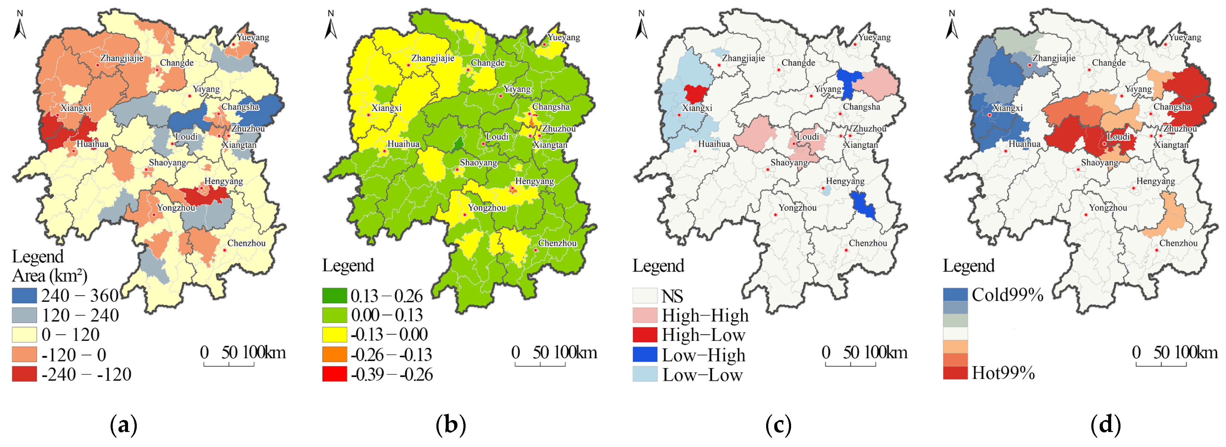
At the prefecture-level city scale, cropland area decreased in three administrative units: Xiangxi Tujia and Miao Autonomous Prefecture (−714.77 km²), Zhangjiajie City (−170.34 km²), and Changde City (−39.73 km²). In contrast, the remaining prefecture-level cities experienced net cropland gains, with an average increase of 353.32 km².

At the county scale, 46 counties experienced a reduction in cropland area, with an average loss of 42.86 km² per county. The largest decreases occurred in Fenghuang County, Mayang Miao Autonomous County—both located in western Hunan (Xiangxi)—and Hengnan County in central Hunan (Xiangzhong). Conversely, 76 counties recorded cropland gains, with an average increase of 64.91 km² per county. The largest increases were observed in Liuyang City and Ningxiang City in northern Hunan (Xiangbei), and Lianyuan City in central Hunan (Xiangzhong).

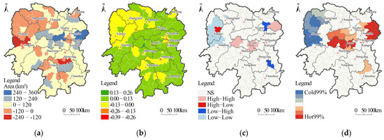
Spatially, counties and prefecture-level cities with net cropland decrease were mainly distributed in western Hunan (Xiangxi) and parts of central Hunan (Xiangzhong), whereas areas with net cropland increase were concentrated primarily in central Hunan (Figure 8a). Based on z-score normalization, the strongest decreases were observed in Furong District and Yuhua District of Changsha City, as well as Yanfeng District and Zhengxiang District of Hengyang City. In contrast, the strongest increase occurred in Lengshuijiang City, a county-level city under the administration of Loudi City (Figure 8b). Spatial autocorrelation analysis further showed that net cropland change was mainly characterized by high–high (HH) and low–low (LL) clustering patterns (Figure 8c). The Global Moran’s I value was 0.23 (z = 3.59, p = 0.000327), indicating statistically significant positive spatial autocorrelation and confirming that net cropland change in Hunan Province followed a non-random clustered spatial pattern. Hotspot–coldspot analysis further identified significant hotspots of net cropland change primarily in central and northern Hunan (Xiangzhong and Xiangbei), whereas coldspots were mainly located in western Hunan (Xiangxi) (Figure 8d).

Figure 8. Analysis of Cropland Change in Hunan Province: (a) Cropland Change Statistics; (b) Normalization; (c) Spatial Clustering Analysis; (d) Hotspot–Coldspot Analysis.

Overall, these spatial diagnostic results reveal the location, clustering characteristics, direction of movement, and spatial concentration of cropland change in Hunan Province. However, these results mainly answer the questions of where cropland change occurred and how it evolved spatially. The underlying socioeconomic mechanisms require further interpretation based on the key factors identified by the XGBoost-SHAP model. And a multicollinearity diagnostic test was conducted before the XGBoost-SHAP analysis. The VIF values of all explanatory variables were below 5, with the maximum VIF being 3.526, indicating no severe multicollinearity among the selected variables. Therefore, all variables were retained in the model. SHAP values were interpreted as predictive contributions rather than independent causal effects.

3.3. Factors Associated with Net Cropland Decrease Based on XGBoost-SHAP

3.3.1. Model Construction and Performance Evaluation

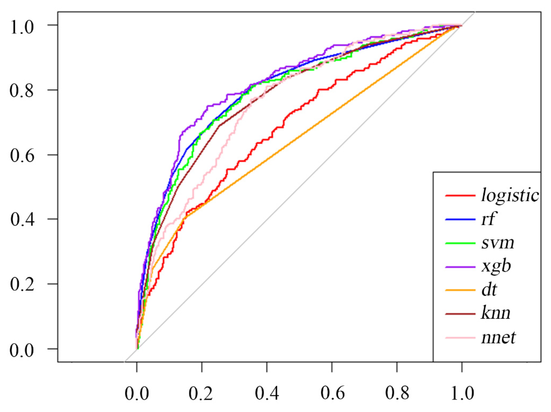
In the XGBoost-SHAP analysis, grid cells with net cropland decrease from 2000 to 2020 were coded as 1, whereas grid cells with net cropland increase or no net change were coded as 0. In the model comparison, XGBoost achieved higher predictive accuracy than Random Forest and Artificial Neural Network models, as indicated by the ROC curves (Figure 9).

Figure 9. ROC Curves of Multiple Models.

In this study, Hunan Province was divided into 2311 non-overlapping 10 km × 10 km grid cells using ArcGIS 10.8 to establish a unified spatial analysis unit for model construction. Spatial overlay calculations were performed for each grid cell to extract cropland change information and match it with the corresponding natural, socioeconomic, and human-activity variables. Based on the binary classification scheme defined above, an XGBoost model was constructed to quantify the relationships between explanatory variables and net cropland decrease at the grid-cell scale. To improve model interpretability and move beyond conventional black-box prediction, SHAP was integrated with XGBoost to evaluate the relative importance, directional associations, nonlinear response patterns, and potential interactions of explanatory variables in relation to the predicted probability of net cropland decrease. This framework enabled both global interpretation of important predictors and local explanation of feature contributions across different grid cells.

Given that cropland change is influenced by multiple interacting natural, socioeconomic, and human-activity factors, a total of 12 explanatory variables were selected based on prior analyses and existing literature. These variables were chosen to reflect the regional characteristics of cropland distribution and change in Hunan Province. Hyperparameter tuning was conducted using grid search combined with five-fold cross-validation, with ROC-AUC used as the optimization metric. The optimal parameter configuration for the XGBoost model was as follows: nrounds = 150, max_depth = 5, eta = 0.01, gamma = 0.25, colsample_bytree = 1, min_child_weight = 1, and subsample = 0.5, with all other parameters set to their default values. A binary logistic objective (objective = “binary:logistic”) was specified for this dichotomous classification task. The optimized model achieved a testing ROC-AUC of 0.899, indicating good predictive performance.

3.3.2. Global Importance and Directional Effects of Predictive Factors

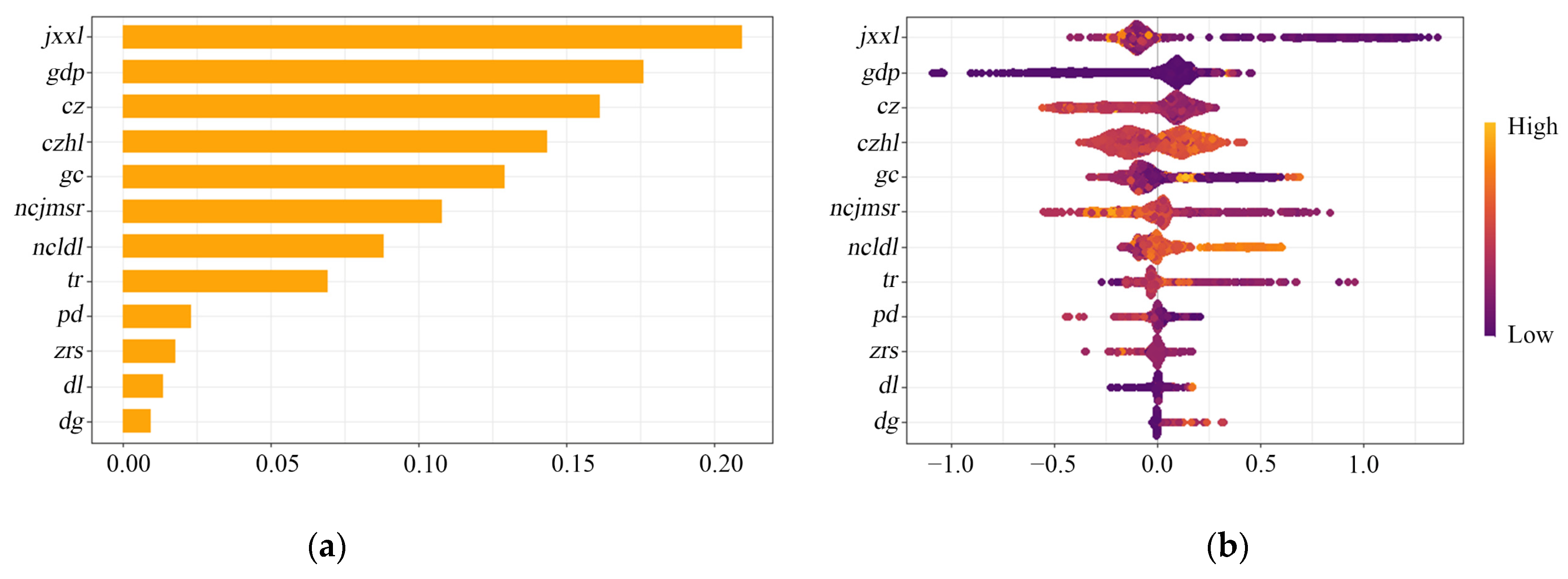
The mean absolute SHAP values were used to rank the relative importance of the 12 explanatory variables associated with cropland change (Figure 10a). The factors were ranked as follows: mechanical efficiency, GDP, fiscal conditions, urbanization rate, elevation, rural residents’ income, rural labor force, soil type, slope, total population, road density, and nighttime light intensity. Overall, socioeconomic and human-activity factors showed higher explanatory contributions than natural factors, indicating that cropland change in Hunan Province was mainly associated with agricultural production capacity, economic development, fiscal conditions, and urbanization. Among these variables, mechanical efficiency had the highest mean absolute SHAP value, suggesting that agricultural mechanization played a key role in shaping cropland change.

Figure 10. Importance and effect direction of predictors for net cropland decrease based on XGBoost-SHAP: (a) importance ranking based on mean absolute SHAP values; (b) SHAP summary plot showing the distribution and direction of feature effects. Note: The factor abbreviations are as follows: jxxl = mechanical efficiency; gdp = gross domestic product; cz = fiscal condition; czhl = urbanization rate; gc = elevation; ncjmsr = rural residents’ income; ncldl = rural labor force; tr = soil type; pd = slope; zrs = total population; dl = road density; and dg = nighttime light intensity. The same abbreviations are used hereafter.

Natural factors had relatively lower SHAP values, but their effects should not be overlooked. In particular, elevation ranked fifth among all variables and accounted for approximately 12% of the total mean absolute SHAP value, indicating that topographic conditions also influenced cropland change in Hunan Province. This is consistent with the province’s complex terrain, where mountainous and hilly areas occupy a large proportion of the land surface and differ substantially from the low-lying plains of northern Hunan.

The SHAP summary plot further illustrates the direction and distribution of feature effects (Figure 10b). Because the model defined cropland decrease as the positive class, positive SHAP values indicate an increased probability of cropland decrease, whereas negative SHAP values indicate a reduced probability. Taking mechanical efficiency as an example, high values of mechanical efficiency were mainly distributed in the negative SHAP region, suggesting that higher mechanization levels tended to reduce the probability of cropland decrease. Conversely, low mechanical efficiency values were mostly associated with positive SHAP values, indicating a higher risk of cropland decrease in less mechanized areas. This pattern may reflect lower agricultural production efficiency, weaker cropland management stability, and a greater likelihood of marginal cropland withdrawal in areas with limited mechanization. However, the SHAP summary plot mainly provides a global overview of feature importance and effect direction. To further examine nonlinear responses and interaction effects among key explanatory variables, SHAP dependence plots, interaction analysis, and heatmaps were used in the subsequent sections.

3.3.3. Nonlinear Associations and Threshold Patterns of Key Explanatory Variables

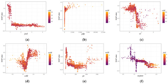
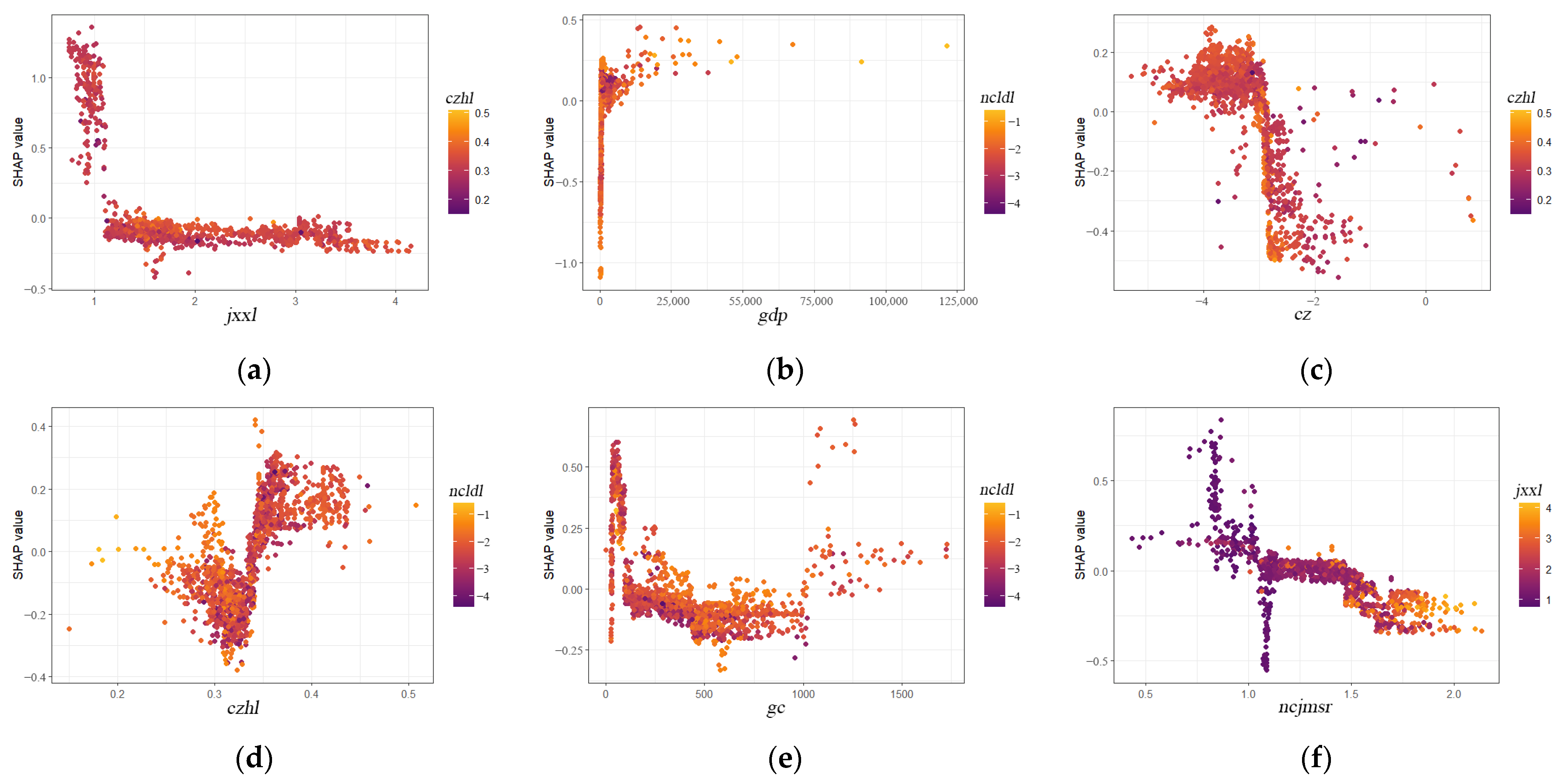
Mechanical efficiency, proxied by agricultural machinery power intensity, was the most important explanatory variable in the model. When mechanical efficiency was below approximately 1.0 (unit: 10⁵ kW per 100 km² grid cell), SHAP values were mostly positive, indicating that low mechanization levels were associated with a higher probability of cropland decrease (Figure 11a). Once mechanical efficiency increased to approximately 1.0–1.2, SHAP values declined rapidly and became negative, suggesting that improved mechanization tended to reduce the probability of cropland decrease. This effect may be related to lower farming costs, higher production efficiency, and more stable cropland management.

Figure 11. SHAP dependence plots of key explanatory variables for net cropland decrease: (a) mechanical efficiency colored by urbanization rate; (b) GDP colored by rural labor force; (c) fiscal condition colored by urbanization rate; (d) urbanization rate colored by rural labor force; (e) elevation colored by rural labor force; and (f) rural residents’ income colored by mechanical efficiency.

GDP showed an overall positive association with cropland decrease. As GDP increased, SHAP values generally tended to rise, indicating that economically developed areas may face stronger pressure from industrial development, urban construction, and infrastructure expansion, thereby increasing the likelihood of the conversion from cropland to non-cropland (Figure 11b). Fiscal conditions exhibited a staged and nonlinear effect. Areas with weaker fiscal capacity were generally associated with positive SHAP values and a higher probability of cropland decrease, whereas stronger fiscal capacity tended to reduce this risk, possibly through agricultural infrastructure investment, land consolidation, and cropland protection measures (Figure 11c). However, stronger fiscal conditions may also be accompanied by greater construction demand, suggesting a potential dual effect on cropland change.

Urbanization rate also exhibited a threshold effect. At low to moderate levels, SHAP values were mostly negative or close to zero, indicating a limited association with cropland decrease. When the urbanization rate exceeded approximately 0.34–0.36, SHAP values became positive, suggesting that urban expansion may increase the probability of conversion from cropland to non-cropland (Figure 11d).

Elevation, the most important natural factor in the model, showed a nonlinear relationship with cropland decrease. Low-elevation areas may be more vulnerable to urban encroachment, whereas mid-elevation areas appeared to maintain relatively stable cropland use. In high-elevation areas, positive SHAP values may reflect cropland decrease associated with poorer farming conditions, fragmented plots, and agricultural marginalization (Figure 11e).

Rural residents’ income was generally associated with a lower probability of cropland decrease. Low-income areas were mostly linked to positive SHAP values, suggesting that insufficient rural income may weaken farmers’ capacity or willingness to maintain cropland. As rural income increased, SHAP values tended to decline and became negative, indicating that higher income levels may support agricultural investment and cropland management stability (Figure 11f). Rural residents’ income and mechanical efficiency may also have a synergistic effect in supporting sustained cropland use.

Overall, the SHAP dependence plots indicate that cropland decrease in Hunan Province was associated with the combined effects of natural conditions, economic development, urban expansion, fiscal capacity, and agricultural production conditions. Mechanical efficiency and rural residents’ income reflect agricultural productivity and management stability; GDP and urbanization rate represent development pressure; fiscal conditions indicate governance and protection capacity; and elevation reflects topographic constraints. These nonlinear and threshold relationships suggest that cropland protection strategies should be region-specific and adapted to local economic, urbanization, fiscal, topographic, and agricultural conditions.

3.3.4. Interaction Patterns and Local Variations Among Explanatory Variables

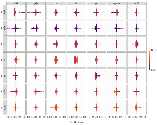
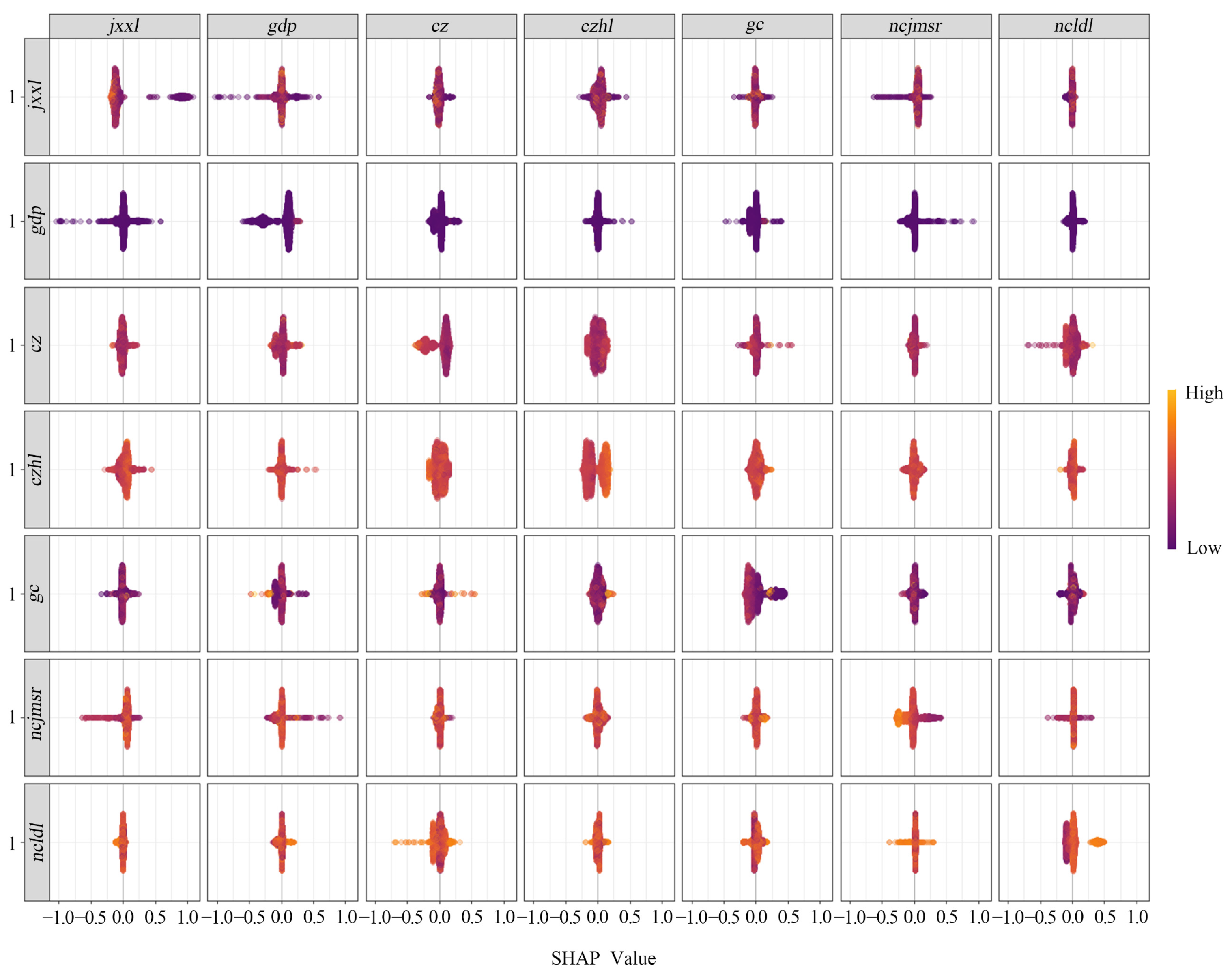
The SHAP interaction matrix further revealed pairwise interaction patterns among the explanatory variables associated with the predicted probability of cropland decrease (Figure 12).

Figure 12. SHAP analysis of pairwise interaction effects among key explanatory variables for net cropland decrease.

Overall, variables such as mechanical efficiency, GDP, elevation, and rural residents’ income showed relatively strong interaction effects with other factors, suggesting that cropland decrease was not determined by individual variables alone but by multiple interacting processes. Among them, mechanical efficiency exhibited the most prominent interactions, particularly with GDP, urbanization rate, and rural residents’ income. This indicates that the effect of agricultural mechanization on cropland decrease may vary under different levels of economic development, urbanization pressure, and rural household income.

GDP and urbanization rate jointly reflected development-related pressure on cropland, whereas fiscal conditions showed a more complex role. Stronger fiscal capacity may support agricultural infrastructure, land consolidation, and cropland protection, but it may also be associated with greater construction demand. Elevation also interacted with socioeconomic variables, suggesting that topographic conditions may modify the effects of economic development and urban expansion on cropland decrease. In low-elevation areas, cropland may be more exposed to urban encroachment, whereas in high-elevation areas, cropland decrease may be related to fragmented plots, poorer farming conditions, and agricultural marginalization. In addition, the interaction between rural residents’ income and mechanical efficiency suggests that improved rural income and mechanization may jointly support more stable cropland use.

These results indicate that cropland decrease in Hunan Province was associated with the combined effects of agricultural production conditions, economic development, urbanization pressure, fiscal capacity, topography, and rural livelihood factors. Therefore, cropland protection strategies should account for regional differences in mechanization level, development stage, urbanization intensity, and terrain conditions.

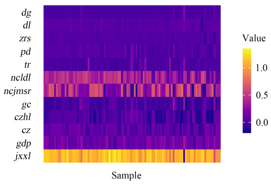
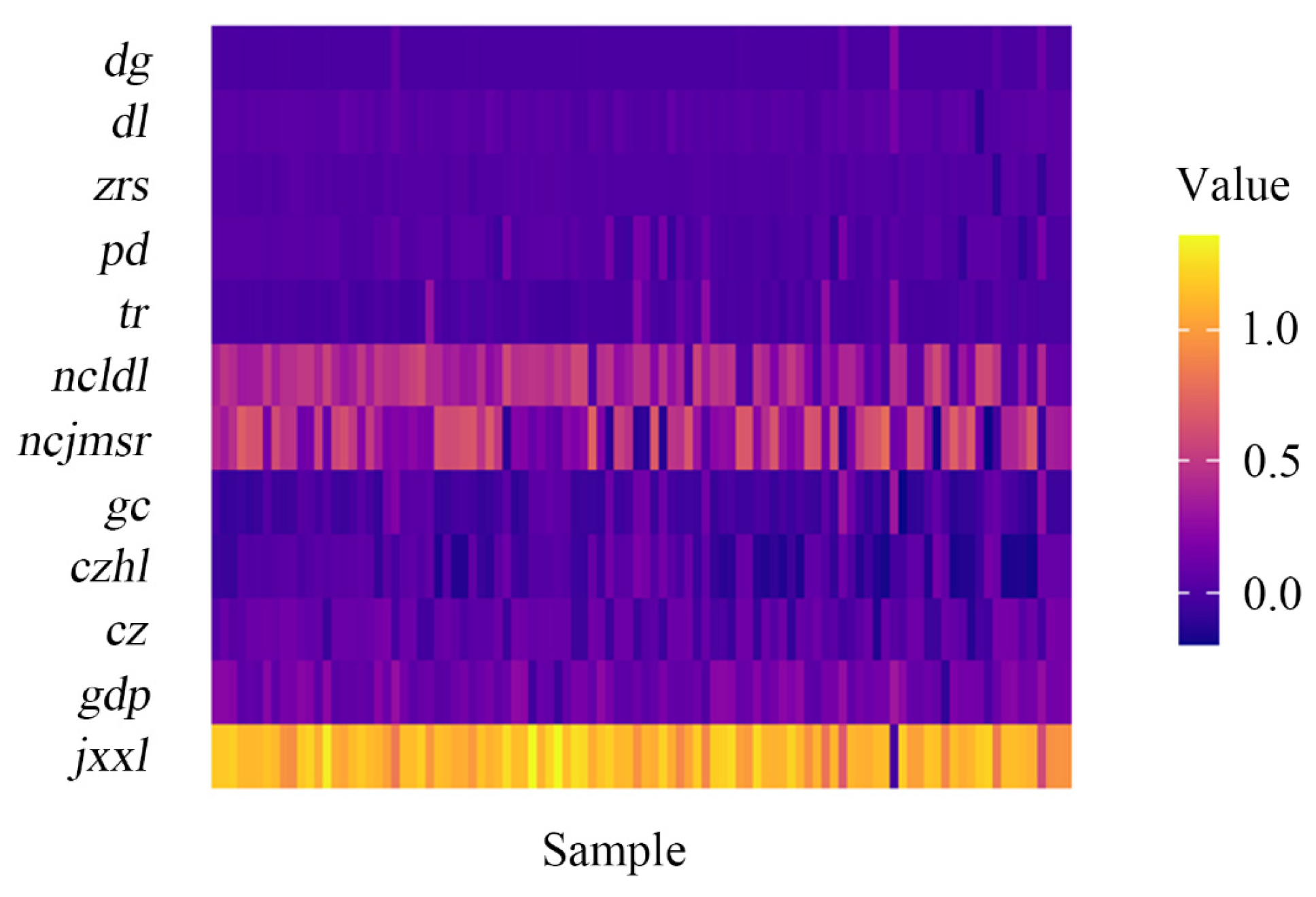
To further examine sample-level heterogeneity in model explanations, the first 100 grid-cell samples were selected for SHAP heatmap analysis (Figure 13). The heatmap shows that socioeconomic and human-activity variables generally contributed more strongly to the model output than most natural variables. In particular, variables such as GDP, fiscal conditions, mechanical efficiency, rural residents’ income, and rural labor force showed relatively high SHAP values across multiple samples, indicating their important roles in explaining the probability of net cropland decrease.

Figure 13. Heatmap Analysis.

Nevertheless, the contribution of natural factors should not be overlooked. Elevation, slope, and soil type also showed noticeable SHAP values in some samples, suggesting that topographic and soil conditions may influence cropland change in specific local contexts. Overall, the heatmap results complement the global importance ranking and interaction analysis by revealing heterogeneous feature contributions at the grid-cell level.

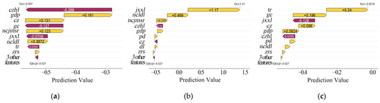
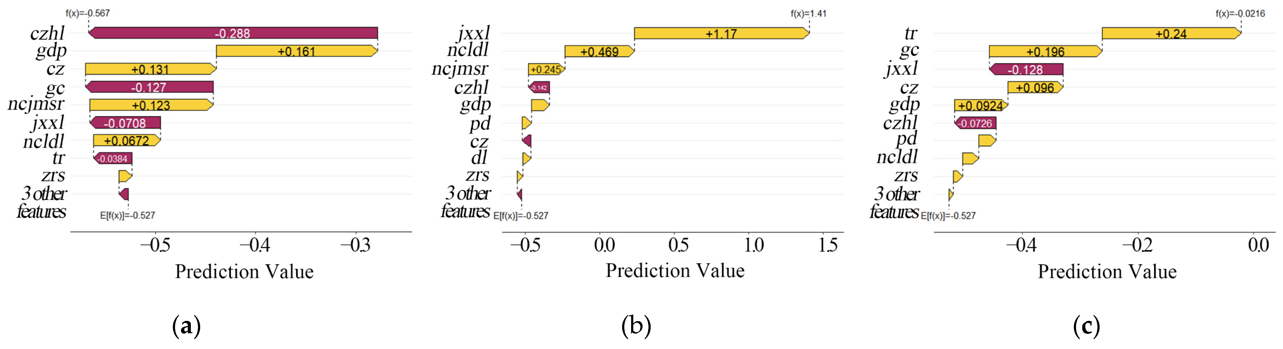
To provide illustrative examples of local variations in feature contributions, three grid-cell cases were selected for case-specific SHAP analysis: one from the western Hunan mountainous region (grid ID: 2249), one from the northern Hunan plain region (grid ID: 1610), and one from the central Hunan hilly-basin region (grid ID: 1838) (Figure 14).

Figure 14. SHAP feature values: (a) Western mountainous region; (b) Northern plain region; (c) Central hilly-basin region.

In the western mountainous region, urbanization rate, GDP, and fiscal conditions showed relatively high SHAP contributions, suggesting that socioeconomic development and urban expansion were closely associated with the probability of net cropland decrease in this area (Figure 14a). This pattern may reflect the continuing demand for infrastructure construction and socioeconomic development in western Hunan.

In the northern plain region, mechanical efficiency showed the strongest contribution to the model output (Figure 14b). This indicates that agricultural mechanization plays an important role in explaining cropland change in the plain region, where large-scale and mechanized agricultural production is more feasible.

In the central hilly-basin region, natural factors, particularly soil type and elevation, showed relatively high SHAP contributions (Figure 14c). This suggests that local topographic and soil conditions may exert a stronger influence on cropland change in hilly-basin areas than in plain regions. Overall, these case-specific examples provide supplementary evidence that feature contributions may vary across local geographic contexts. However, the broader relationships among socioeconomic, agricultural, and natural factors are mainly supported by the global SHAP importance ranking, interaction analysis, and heatmap results.

4. Discussion

The 2025 No. 1 Central Document of the Communist Party of China and the State Council, Opinions on Further Deepening Rural Reforms and Solidly Promoting Comprehensive Rural Revitalization, emphasizes the need to strengthen the supply security of grain and other key agricultural products, stabilize the grain-sown area, reinforce cropland protection, and improve cropland quality. Hunan Province accounts for 2.8% of China’s total cropland area, contributes 4.5% of national grain production, and produces 12.2% of the country’s rice output. As one of China’s major grain-producing provinces, Hunan plays an important role in maintaining national food security and stabilizing cropland resources. In addition, the Hunan Province Farmland Protection Special Plan for Territorial Space (2021–2035) highlights the need to promote high-quality cropland protection and efficient cropland utilization, and to develop permanent basic farmland into concentrated, contiguous, high-standard farmland with stable yields and strong resistance to drought and flooding.

Based on the empirical results and regional characteristics identified in this study, three policy implications can be proposed.

First, cropland quantity, quality, and productivity should be stabilized and improved simultaneously. The results show that Hunan’s total cropland area has declined since its peak in 2009, and that the spatial concentration of cropland outflow is generally stronger than that of cropland inflow. This suggests that cropland protection should not focus only on compensating for area loss, but should also emphasize the quality and productivity of newly added or restored cropland. In particular, northern Hunan’s plain region and central Hunan’s hilly-basin region should be prioritized for cropland consolidation and high-standard farmland construction. As mechanical efficiency increases, cropland protection policies should further coordinate improvements in cropland quality, mechanized production capacity, and grain yield stability.

Second, county-level urban–rural planning should be strengthened. The SHAP results indicate that mechanical efficiency and urbanization rate are important factors associated with net cropland decrease. In some areas, rapid urbanization and construction expansion may increase pressure on cropland, whereas insufficient rural infrastructure may limit agricultural modernization. Therefore, county-level planning should better coordinate urban expansion, rural infrastructure improvement, and agricultural production space. In areas with low road density and weak nighttime light intensity, targeted investment in rural infrastructure may provide necessary material support for agricultural modernization and the development of new-generation agricultural operators.

Third, differentiated cropland protection strategies should be adopted according to regional conditions. The SHAP analysis shows that the dominant factors associated with net cropland decrease vary across western mountainous areas, northern plain areas, and central hilly-basin areas. In western Hunan, where terrain constraints are strong and socioeconomic development remains uneven, cropland protection should balance urbanization demand with the conservation of suitable cropland resources. In northern Hunan’s plain areas, policy efforts should focus on large-scale, mechanized, and high-standard farmland construction. In central Hunan’s hilly-basin areas, greater attention should be paid to soil quality, terrain suitability, and farmland improvement measures, including the conversion of suitable dryland into paddy fields where appropriate. Overall, cropland protection in Hunan Province should integrate spatial planning, agricultural modernization, and region-specific land management measures.

Despite these contributions, this study has several limitations.

(1) Although the 10 km × 10 km grid provided a consistent unit for integrating multi-source data, it may obscure fine-scale land-use heterogeneity. In addition, the significant Moran’s I values suggest spatial dependence among grid cells, which was not explicitly modelled in the XGBoost-SHAP framework. Thus, the results should be interpreted as model-based associations rather than causal effects, and future studies should consider alternative grid resolutions and spatially explicit modelling approaches.

(2) Although the analysis was conducted in Hunan Province, the findings should be understood through transferable regional characteristics, including terrain conditions, urbanization intensity, socioeconomic development, agricultural mechanization, and cropland suitability, rather than through place-specific divisions alone.

(3) The selected variables captured multiple dimensions of cropland change, but some relevant factors, such as land prices and urban accessibility, were not included because of limited long-term gridded data availability. Future research could incorporate more refined land-market and accessibility variables when comparable datasets become available.

5. Conclusions

This study examined cropland change in Hunan Province from two perspectives: the spatiotemporal patterns of cropland change and the factors associated with net cropland decrease. The main conclusions are as follows:

(1) From 2000 to 2020, the total cropland area in Hunan Province showed an inverted U-shaped trajectory, increasing initially and then decreasing. Cropland area increased continuously from 2000 to 2009, followed by a decline after reaching its peak in 2009. Based on county-level statistics and hotspot–coldspot analysis, areas with net cropland decrease were mainly distributed in western Hunan and parts of central Hunan, whereas areas with net cropland increase were concentrated primarily in central Hunan.

(2) Cropland outflow showed stronger spatial concentration than cropland inflow. The Lorenz curve and Gini coefficient results based on five-year intervals indicate that the spatial imbalance of cropland outflow gradually decreased over time, whereas that of cropland inflow first declined and then slightly increased in the final period.

(3) The XGBoost-SHAP results show that socioeconomic and human-activity factors generally made greater contributions to net cropland decrease than natural factors. The explanatory variables were ranked by mean absolute SHAP value as follows: mechanical efficiency > GDP > fiscal conditions > urbanization rate > elevation > rural residents’ income > rural labor force > soil type > slope > total population > road density > nighttime light intensity.

(4) SHAP dependence and interaction analyses revealed nonlinear responses, threshold patterns, and interaction effects among key explanatory variables. Mechanical efficiency, GDP, fiscal conditions, urbanization rate, elevation, and rural residents’ income showed nonlinear effects on the probability of net cropland decrease. Interactions such as mechanical efficiency × GDP, rural residents’ income × mechanical efficiency, and rural residents’ income × GDP played important roles in explaining spatial differences in cropland change.

(5) Case-specific SHAP analysis of three illustrative grid cells showed that the dominant factors associated with net cropland decrease varied across regional contexts. In western Hunan’s mountainous region, urbanization rate, GDP, and fiscal conditions showed relatively high SHAP contributions. In northern Hunan’s plain region, mechanical efficiency made the strongest contribution. In central Hunan’s hilly-basin region, natural factors, especially soil type and elevation, showed relatively high contributions. These findings indicate that cropland protection policies in Hunan Province should be region-specific and should account for differences in socioeconomic development, agricultural mechanization, and natural conditions.

Beyond these empirical findings, this study contributes to the literature in three main aspects. First, from a methodological perspective, it demonstrates the usefulness of integrating XGBoost with SHAP for identifying nonlinear and interactive relationships between cropland change and multiple associated factors, thereby improving the interpretability of machine-learning-based land-use change analysis. Second, from an empirical perspective, it provides grid-scale evidence on the spatiotemporal dynamics of cropland change and the relative importance of socioeconomic, agricultural, and natural factors associated with net cropland decrease in a major grain-producing province. Third, from a practical perspective, the findings provide evidence-based implications for differentiated cropland protection, agricultural mechanization, and land-use management under different geographic and socioeconomic conditions.

References

- He, A.; Li, J.; Long, J.; Ai, Z.; Zhang, P.; Guo, X. Spatial and Temporal Variations of Climate Resources during the Growing Season of Early-Season Rice in Hunan Province. Agriculture 2024, 14, 1514. [Google Scholar] [CrossRef] [Scilit]
- Hu, P.; Peng, C.; Chen, C. Hunan Leads Nation in Early Rice Planting Area and Total Output. Hunan Daily, 27 August 2024; p. 1.
- Yu, D.; Yu, S.; He, Q.; Li, C.; Wei, C. Monitoring of Dongting Lake Atrophy in the Past 100 Years by Combining Historical Map and Remote Sensing Technology. Remote Sens. Land Resour. 2016, 28, 116–122. [Google Scholar]
- Zhao, C.; Zhou, Y.; Li, X.; Xiao, P.; Jiang, J. Assessment of Cultivated Land Productivity and Its Spatial Differentiation in Dongting Lake Region: A Case Study of Yuanjiang City, Hunan Province. Sustainability 2018, 10, 3616. [Google Scholar] [CrossRef] [Scilit]
- Lin, D.; Tang, H. Current Status and Governance Strategies for Farmland Fragmentation: A Case Study of Town R, Hunan Province. Rural Econ. Technol. 2024, 35, 30–34. [Google Scholar]
- Tian, Y. Building Homes and Careers: The Operational Logic of Returning Youth “Re-Agriculturalization”. Theory Mon. 2024, 138–147. [Google Scholar] [CrossRef]
- Wang, L. A Narrative Study of Why Young People Go “Back-to-the-Land”: Interpretation from the Perspective of Self-Identity Theory. J. Rural Stud. 2025, 120, 103832. [Google Scholar]
- Huang, Q.; Guo, W.; Wang, Y. A Study of the Impact of New Quality Productive Forces on Agricultural Modernization: Empirical Evidence from China. Agriculture 2024, 14, 1935. [Google Scholar] [CrossRef] [Scilit]
- Viana, C.M.; Freire, D.; Abrantes, P.; Rocha, J.; Pereira, P. Agricultural Land Systems Importance for Supporting Food Security and Sustainable Development Goals: A Systematic Review. Sci. Total Environ. 2022, 806, 150718. [Google Scholar] [CrossRef] [Scilit] [PubMed]
- Bren d’Amour, C.; Reitsma, F.; Baiocchi, G.; Barthel, S.; Güneralp, B.; Erb, K.-H.; Haberl, H.; Creutzig, F.; Seto, K.C. Future urban land expansion and implications for global croplands. Proc. Natl. Acad. Sci. USA 2017, 114, 8939–8944. [Google Scholar] [PubMed]
- Lu, X.; Zhang, Y.; Zou, Y. Evaluation the Effect of Cultivated Land Protection Policies Based on the Cloud Model: A Case Study of Xingning, China. Ecol. Indic. 2021, 131, 108247. [Google Scholar] [CrossRef] [Scilit]
- Wang, X.; Hu, H.; Ning, A.; Li, G.; Wang, X. The Impact of Farmers’ Perception on Their Cultivated Land Quality Protection Behavior: A Case Study of Ningbo, China. Sustainability 2022, 14, 6357. [Google Scholar] [CrossRef] [Scilit]
- Yu, D.; Hu, S.; Tong, L.; Xia, C. Spatiotemporal Dynamics of Cultivated Land and Its Influences on Grain Production Potential in Hunan Province, China. Land 2020, 9, 510. [Google Scholar] [CrossRef] [Scilit]
- Lambin, E.F.; Turner, B.L., II; Geist, H.J.; Agbola, S.B.; Angelsen, A.; Bruce, J.W.; Coomes, O.T.; Dirzo, R.; Fischer, G.; Folke, C.; et al. The Causes of Land-Use and Land-Cover Change: Moving beyond the Myths. Glob. Environ. Change 2001, 11, 261–269. [Google Scholar]
- Verburg, P.H.; Crossman, N.; Ellis, E.C.; Heinimann, A.; Hostert, P.; Mertz, O.; Nagendra, H.; Sikor, T.; Erb, K.-H.; Golubiewski, N.; et al. Land System Science and Sustainable Development of the Earth System: A Global Land Project Perspective. Anthropocene 2015, 12, 29–41. [Google Scholar] [CrossRef] [Scilit]
- Winkler, K.; Fuchs, R.; Rounsevell, M.; Herold, M. Global Land Use Changes Are Four Times Greater than Previously Estimated. Nat. Commun. 2021, 12, 2501. [Google Scholar] [CrossRef] [Scilit] [PubMed]
- Yang, F.; Dong, G.; Wu, P.; He, F. Stylized Facts of Past 1000-Year of China’s Cropland Changes. Land Use Policy 2024, 144, 107258. [Google Scholar] [CrossRef] [Scilit]
- Hu, Y.; Batunacun; Zhen, L.; Zhuang, D. Assessment of Land-Use and Land-Cover Change in Guangxi, China. Sci. Rep. 2019, 9, 2189. [Google Scholar] [PubMed]
- Liu, J.; Kuang, W.; Zhang, Z.; Xu, X.; Qin, Y.; Ning, J.; Zhou, W.; Zhang, S.; Li, R.; Yan, C.; et al. Spatiotemporal characteristics, patterns, and causes of land-use changes in China since the late 1980s. J. Geogr. Sci. 2014, 24, 195–210. [Google Scholar] [CrossRef] [Scilit]
- Wang, Y.; Song, D.; Liu, C.; Li, S.; Yuan, M.; Gong, J.; Yang, J. Spatial Correlation of Non-Agriculturalization and Non-Grain Utilization Transformation of Cultivated Land in China and Its Implications. Land 2025, 14, 1031. [Google Scholar]
- Lu, D.; Wang, Z.; Su, K.; Zhou, Y.; Li, X.; Lin, A. Understanding the Impact of Cultivated Land-Use Changes on China’s Grain Production Potential and Policy Implications: A Perspective of Non-Agriculturalization, Non-Grainization, and Marginalization. J. Clean. Prod. 2024, 434, 140647. [Google Scholar]
- Cui, J.; Jin, H.; Luo, Y.; Lin, Y.; Tong, X.; Zhu, Y. Non-Agricultural Transformation and Non-Grain Production and Their Coordinated Relationships with Rural Population Hollowing: A Case Study of Yangtze River Economic Belt. Acta Ecol. Sin. 2024, 44, 1822–1836. [Google Scholar]
- Liu, W. Spatial Characteristics and Driving Factors of Non-Agricultural Use of Farmland in Northeast China. Master’s Thesis, Jilin Agricultural University, Changchun, China, 2024. [Google Scholar]
- Zhu, H.; Li, Y. Empirical Analysis of the Causes of Farmland Expansion in Arid Regions of Northwest China. Prog. Geogr. 2011, 30, 615–620. [Google Scholar]
- Wan, F.; Deng, Q.; Liu, L.; Li, P.; Yang, X. Spatiotemporal Evolution of Cultivated Land in the Hehuang Valley from 1990 to 2018. Bull. Soil Water Conserv. 2021, 41, 275–282. [Google Scholar]
- Yu, W.; Wu, T.; Luo, Y.; Li, X. Spatiotemporal Patterns of Farmland Evolution and Their Driving Mechanisms in the Urbanization Process: A Case Study of Yangzhou City. J. Southwest Univ. Nat. Sci. Ed. 2023, 45, 147–159. [Google Scholar]
- Zhang, G.; Li, X.; Zhang, L.; Wei, X. Dynamics and Causes of Cropland Non-Agriculturalization in Typical Regions of China: An Explanation Based on Interpretable Machine Learning. Ecol. Indic. 2024, 166, 112348. [Google Scholar] [CrossRef] [Scilit]
- Wu, X.; Zhao, N.; Wang, Y.; Zhang, L.; Wang, W.; Liu, Y. Cropland Non-Agriculturalization Caused by the Expansion of Built-Up Areas in China during 1990–2020. Land Use Policy 2024, 146, 107312. [Google Scholar]
- Gui, S.; Li, J.; Chen, G.; Zhao, J.; Tang, B.; Li, L. Identification of Abandoned Cropland and Global–Local Driving Mechanism Analysis via Multi-Source Remote Sensing Data and Multi-Objective Optimization. Remote Sens. 2025, 17, 3086. [Google Scholar]
- Zhang, L.; Lu, D.; Li, Q.; Lu, S. Impacts of Socioeconomic Factors on Cropland Transition and Its Adaptation in Beijing, China. Environ. Earth Sci. 2018, 77, 575. [Google Scholar] [CrossRef] [Scilit]
- Yan, H.; Chen, H.; Wang, F.; Qiu, L. Dynamics of Cropland Non-Agriculturalization in Shaanxi Province of China and Its Attribution Using a Machine Learning Approach. Land 2025, 14, 190. [Google Scholar] [CrossRef] [Scilit]
- Batunacun; Wieland, R.; Lakes, T.; Nendel, C. Using Shapley Additive Explanations to Interpret Extreme Gradient Boosting Predictions of Grassland Degradation in Xilingol, China. Geosci. Model Dev. 2021, 14, 1493–1510. [Google Scholar] [CrossRef] [Scilit]
- Mao, C.; Feng, S.; Zhou, C. Cropland Loss under Different Urban Expansion Patterns in China (1990–2020): Spatiotemporal Characteristics, Driving Factors, and Policy Implications. Land 2025, 14, 343. [Google Scholar] [CrossRef] [Scilit]
- Han, H.; Peng, H.; Li, S.; Yang, J.; Yan, Z. The Non-Agriculturalization of Cultivated Land in Karst Mountainous Areas in China. Land 2022, 11, 1727. [Google Scholar] [CrossRef] [Scilit]
- Aas, K.; Jullum, M.; Løland, A. Explaining Individual Predictions When Features Are Dependent: More Accurate Approximations to Shapley Values. Artif. Intell. 2021, 298, 103502. [Google Scholar] [CrossRef] [Scilit]
- Janzing, D.; Minorics, L.; Blöbaum, P. Feature Relevance Quantification in Explainable AI: A Causal Problem. In Proceedings of the Twenty Third International Conference on Artificial Intelligence and Statistics, Palermo, Italy, 26–28 August 2020; pp. 2907–2916. [Google Scholar]
- Kumar, I.E.; Venkatasubramanian, S.; Scheidegger, C.; Friedler, S. Problems with Shapley-Value-Based Explanations as Feature Importance Measures. In Proceedings of the 37th International Conference on Machine Learning, Online, 13–18 July 2020; pp. 5491–5500. [Google Scholar]
- Yang, J.; Huang, X. The 30 m Annual Land Cover Dataset and Its Dynamics in China from 1990 to 2019. Earth Syst. Sci. Data 2021, 13, 3907–3925. [Google Scholar] [CrossRef] [Scilit]
- Moran, P.A.P. Notes on Continuous Stochastic Phenomena. Biometrika 1950, 37, 17–23. [Google Scholar] [CrossRef] [Scilit] [PubMed]
- Anselin, L. Local Indicators of Spatial Association—LISA. Geogr. Anal. 1995, 27, 93–115. [Google Scholar] [CrossRef] [Scilit]
- Getis, A.; Ord, J.K. The Analysis of Spatial Association by Use of Distance Statistics. Geogr. Anal. 1992, 24, 189–206. [Google Scholar] [CrossRef] [Scilit]
- Yuill, R.S. The Standard Deviational Ellipse; An Updated Tool for Spatial Description. Geogr. Ann. Ser. B Hum. Geogr. 1971, 53, 28–39. [Google Scholar] [CrossRef]
- Wang, B.; Shi, W.; Miao, Z. Confidence Analysis of Standard Deviational Ellipse and Its Extension into Higher Dimensional Euclidean Space. PLoS ONE 2015, 10, e0118537. [Google Scholar] [CrossRef] [Scilit] [PubMed]
- Zheng, X.; Xia, T.; Yang, X.; Yuan, T.; Hu, Y. The Land Gini Coefficient and Its Application for Land Use Structure Analysis in China. PLoS ONE 2013, 8, e76165. [Google Scholar] [CrossRef] [Scilit] [PubMed]
- Yan, F.; Zhang, S.; Liu, X.; Chen, D.; Chen, J.; Bu, K.; Yang, J.; Chang, L. The Effects of Spatiotemporal Changes in Land Degradation on Ecosystem Services Values in Sanjiang Plain, China. Remote Sens. 2016, 8, 917. [Google Scholar] [CrossRef] [Scilit]
- Chen, T.; Guestrin, C. XGBoost: A Scalable Tree Boosting System. In Proceedings of the 22nd ACM SIGKDD International Conference on Knowledge Discovery and Data Mining, San Francisco, CA, USA, 13–17 August 2016; pp. 785–794. [Google Scholar]
- Lundberg, S.M.; Lee, S.-I. A Unified Approach to Interpreting Model Predictions. In Proceedings of the 31st International Conference on Neural Information Processing Systems, Long Beach, CA, USA, 4–9 December 2017; pp. 4765–4774. [Google Scholar]
- Guidotti, R.; Monreale, A.; Ruggieri, S.; Turini, F.; Giannotti, F.; Pedreschi, D. A Survey of Methods for Explaining Black Box Models. ACM Comput. Surv. 2019, 51, 93. [Google Scholar]
- Lundberg, S.M.; Erion, G.; Chen, H.; DeGrave, A.; Prutkin, J.M.; Nair, B.; Katz, R.; Himmelfarb, J.; Bansal, N.; Lee, S.-I. From Local Explanations to Global Understanding with Explainable AI for Trees. Nat. Mach. Intell. 2020, 2, 56–67. [Google Scholar] [CrossRef] [Scilit] [PubMed]
Disclaimer/Publisher’s Note: The statements, opinions and data contained in all publications are solely those of the individual author(s) and contributor(s) and not of MDPI and/or the editor(s). MDPI and/or the editor(s) disclaim responsibility for any injury to people or property resulting from any ideas, methods, instructions or products referred to in the content. |
© 2026 by the authors. Licensee MDPI, Basel, Switzerland. This article is an open access article distributed under the terms and conditions of the Creative Commons Attribution (CC BY) license.