Research on the Influence Mechanism of Urban Morphology Indicators on the Diurnal and Seasonal Surface Temperature

Abstract

Urban morphology influences the distribution and variation of land surface temperature (LST) by altering surface cover type. However, the coupling effects of the daily LST cycle and the multidimensional morphological driving mechanisms remain insufficiently explored in existing studies. This study, based on ECOSTRESS diurnal LST data, focuses on Harbin, a representative city in China’s cold climate regions. By integrating land cover data, urban morphology vector data, and interpretable machine learning models, it investigates the intricate relationship between urban morphology indicators and LST over a 24 h cycle under cold climate conditions. LST prediction was carried out using Gradient Boosting Decision Trees (XGBoost), Random Forests (RF), Support Vector Machines (SVM), and Multiple Linear Regression (MLR), with an evaluation of the prediction accuracy of each model. The findings indicated the following: (1) The influence of 2D and 3D urban morphological indicators on LST exhibits significant seasonal variation, with Building Otherness (BO), Mean Building Height (BH), and the Normalized Difference Vegetation Index (NDVI) exerting notable impacts on LST in both winter and summer. (2) Significant interactions exist between certain urban morphological indicators that can effectively reduce LST, when the Patch Land Area Proportion (PLAND) exceeds 40%, increasing the Largest Patch Index (LPI) contributes to lowering LST in summer. (3) Among the evaluated machine learning algorithms, XGBoost demonstrates the highest prediction accuracy. This study provides scientific insights for urban planning and policy development, aiding in the optimization of urban morphological designs to effectively regulate LST.

1. Introduction

With the acceleration of urbanization, natural landscapes are increasingly replaced by impervious surfaces, resulting in significant changes to the urban thermal environment [1]. Land Surface Temperature (LST) serves as a key indicator for assessing changes in urban thermal systems and their degree of warming [2]. LST is influenced by various factors, including seasonal variations, temporal factors, the proportion of impervious areas, and vegetation cover [3]. In recent years, climatologists have shifted their focus to the impact of anthropogenic factors on local climates to better understand these influences on LST [4,5]. Existing studies have shown that changes in landscape and urban structure resulting from urban expansion and renewal are primary drivers of LST increase, significantly affecting the internal temperature distribution of cities [6,7]. Therefore, a quantitative analysis of urban morphology is essential for understanding its relationship with LST.

A variety of urban morphology parameters have been proposed to reveal the relationship between urban morphology and LST, providing scientific insights for urban planning [8]. Among these, increasing urban green spaces is considered one of the most common and effective methods for mitigating heat [9]. Green spaces reduce the direct exposure of the surface to solar radiation through shading and lower air temperature via evapotranspiration. Urban green spaces including green roofs, courtyard gardens, urban forests, roadside greenery, and scattered trees, shrubs, and grass, all of which have been proven to have significant cooling effects at the local scale [10]. In addition to nature-based measures, factors such as building density, form, and layout also significantly influence LST [11]. Two-dimensional (2D) urban morphology indicators, such as urban green cover ratio and impervious surface area, are key factors affecting spatial variation in LST. Recent studies have indicated that incorporating three-dimensional (3D) urban morphology factors can improve the explanatory power of LST variation by approximately 20% [12,13]. These findings have deepened the understanding of the mechanisms by which urban morphology influences LST. However, the precise impact of 2D and 3D urban morphology indicators on hourly LST remains unclear.

Remote sensing inversion is a commonly used technique in urban thermal environment studies [14]. Satellites such as Landsat, MODIS, ASTER, and HJ-1B provide rapid access to urban thermal environment data. However, polar-orbiting satellites lack the ability to capture both day and night data, making it difficult to fully monitor the temporal changes in the urban heat environment, thus hindering a comprehensive understanding of the daily dynamics of LST and its driving factors [15]. This limitation can be addressed by the data from the Ecosystem Spaceborne Thermal Radiometer Experiment on Space Station (ECOSTRESS), which provides the highest spatial resolution (38 m × 69 m) thermal infrared data currently available and covers multiple time periods throughout the day and night. ECOSTRESS has been widely applied in urban thermal environment research [16,17,18]. LST is influenced by a combination of factors, including solar radiation, surface material properties, and urban morphology, and exhibits significant dynamic fluctuations over the day-night cycle. Studying hourly LST variations helps to identify periods of high temperatures and spatial distribution patterns, advancing the understanding of the mechanisms behind urban thermal processes and providing more precise scientific evidence for heat environment prediction and urban planning regulation.

There exists a complex interaction between LST and urban morphology parameters [19]. While existing studies have explored the relationship between urban morphology parameters and LST, the contribution weights of different indicators have not yet been thoroughly analyzed [20,21]. Most current studies rely on linear relationship analysis, correlation coefficients, or linear regression models to investigate the relationship between urban morphology and LST. However, these methods fail to capture the intricate nonlinear interactions comprehensively [22]. Therefore, machine learning algorithms, such as Random Forest (RF) and Gradient Boosting Trees (GBRT), offer a promising approach to overcome the limitations of traditional linear models, enabling a deeper analysis of the factors influencing LST variations.

Machine learning, grounded in statistical learning theory, offers innovative methods for high-precision LST prediction by constructing adaptive algorithms that analyze the spatial and temporal heterogeneity of LST [23,24]. In LST prediction tasks, different models exhibit varying performance due to differences in their algorithmic structure and data adaptability. Model selection is influenced not only by the prediction objectives and sample size but also by the climate context and characteristic indicators of the study area. Extreme Gradient Boosting (XGBoost), based on the gradient boosting mechanism and regularization strategies, demonstrates high predictive accuracy in modeling complex nonlinear feature interactions and offers strong interpretability. However, it has limitations in time series modeling and handling spatial autocorrelation [25]. Long Short-Term Memory (LSTM), relying on a gating mechanism, effectively captures the temporal dynamics of LST but incurs high computational costs for large-scale training data and is prone to overfitting in data-sparse regions [26]. RF, by integrating multiple decision trees, enhances predictive accuracy and robustness, efficiently handling high-dimensional data and noise interference. However, it is sensitive to highly correlated features and has high computational costs [27]. Support Vector Machine (SVM) performs well in small sample and high-dimensional data environments, particularly suited for regression tasks in complex feature spaces. However, its training efficiency on large datasets is low, and the parameter tuning process is complex, making it less suited for large-scale spatiotemporal predictions [28]. Although various machine learning models have been applied to LST prediction, fine-scale prediction studies, especially for extremely cold cities, remain relatively scarce. There is a lack of horizontal comparison and performance evaluation of different models in such regions. Therefore, exploring the adaptability and optimization strategies of models in cold regions is crucial for improving LST simulation accuracy and understanding its spatial variation mechanisms. A rational selection and optimization of predictive models will help achieve refined LST regulation and provide regionally adaptive technical support.

Existing studies have explored the influence of urban morphology on LST from different perspectives; however, several limitations remain. Most studies focus on daily mean or extreme LST values, while limited attention has been paid to the diurnal variability of LST and its underlying driving mechanisms. In addition, the integrated representation of multidimensional 2D and 3D urban morphology indicators and their interaction mechanisms has not been sufficiently examined, and the applicability of different machine learning models under complex urban forms and varying climatic conditions remains inadequately evaluated, particularly for cold-climate cities. Against this background, this study focuses on the cold-region city of Harbin and integrates high-resolution ECOSTRESS LST data with multidimensional 2D and 3D urban morphology indicators to systematically characterize the dynamic effects of urban morphology on summer and winter LST at an hourly scale, thereby addressing existing gaps in temporal resolution and climatic context. Moreover, a comparative analysis of multiple machine learning models is conducted to reduce uncertainties associated with a single modeling approach and to enhance the robustness and reliability of LST prediction results. Accordingly, the objectives of this study are to: (1) quantify the contributions of 2D and 3D urban morphology indicators to hourly LST variations; (2) analyze the interaction mechanisms among key morphological indicators and derive implications for urban planning; and (3) evaluate the applicability of different machine learning models for LST prediction in cold-climate cities.

2. Materials and Methods

2.1. Study Area

Harbin (125°42′–130°44′ E longitude, 10°04′–46°40′ N latitude) is the capital of Heilongjiang province and the largest city in northeastern China. The city has a temperate continental monsoon climate, with long and cold winters (November to March), where the average temperature is −19 °C, and short and hot summers (July to August), with an average temperature of 23 °C [29].

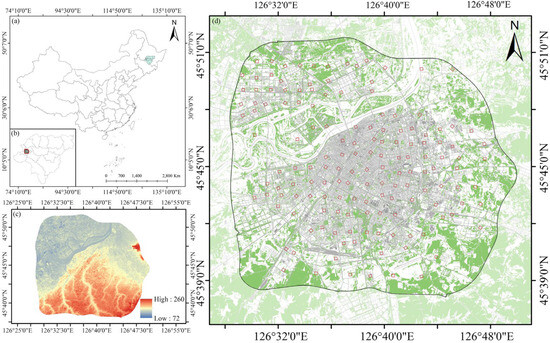
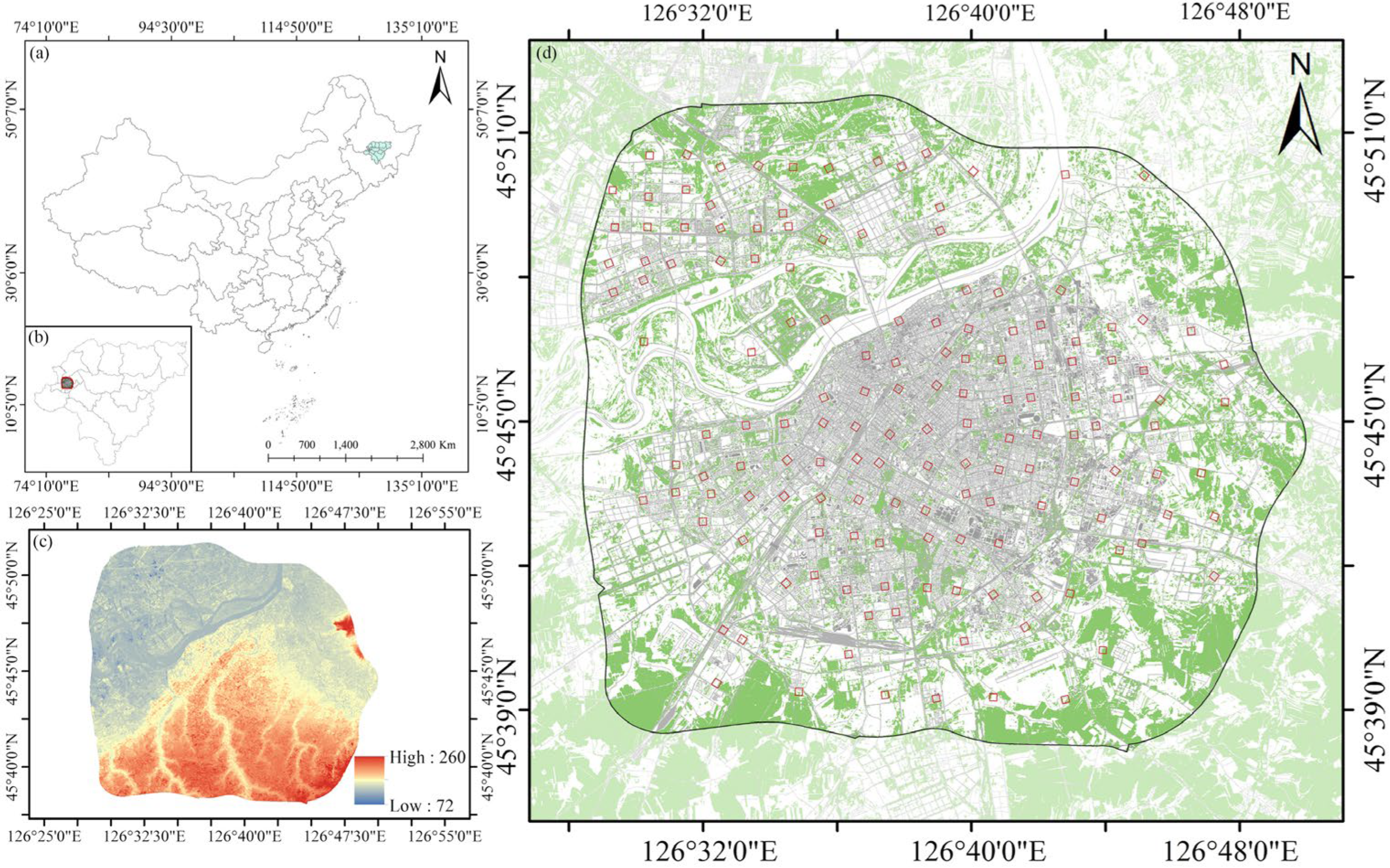
Harbin consists of nine urban districts and nine county-level cities. The urban development pattern is characterized by a series of traffic rings, including the first, second, third, and fourth ring roads. The primary built-up area is located within the fourth ring road, while the building density significantly decreases beyond this area. Given that most social activities are concentrated within this zone, studying this area is crucial for assessing the impact of recent urban development on the environment. The total study area spans approximately 592.3 km², with the main street blocks arranged in a 400 m × 400 m grid. The streets predominantly follow southeast-northwest and northeast-southwest orientations [30]. The study area is shown in Figure 1.

Figure 1. (a) Geographical distribution of Harbin in China. (b) The geographical location of the study area in Harbin. (c) Elevation distribution map of the research area. (d) The geographic distribution of sample blocks.

2.2. Urban Morphological Metrics Measurement and Computation

To systematically investigate the impact of urban morphology on LST, a comprehensive set of 20 urban morphology parameters was selected based on a rational and scientifically sound sampling design. Indicators were selected according to their frequent use in previous urban climate and morphology studies, distinct spatial interpretations, and limited redundancy among variables.

The study area was sampled using a random selection of 150 blocks, each with a size of 400 m × 400 m. The 400 m × 400 m block size corresponds to the typical urban block scale defined by Harbin’s road network and is suitable for representing neighborhood-level urban morphology. Given that the spatial resolution of ECOSTRESS LST data is approximately 70 m, each sampling unit contains several LST pixels, allowing LST values to be summarized at the block level for subsequent analysis. Although spatial autocorrelation may still exist in urban environmental variables, the use of randomly distributed sampling blocks helps reduce potential spatial dependence among samples, and a detailed assessment of spatial autocorrelation is conducted in Section 2.4. The selected urban morphology indicators, including both 2D and 3D parameters, are summarized in Table 1 and were chosen with reference to previous studies in the field [31,32,33,34]. Landscape pattern indicators were computed using FRAGSTATS 4.2, while NDVI and building morphology parameters were calculated in ArcGIS 10.7. Leaf area index (LAI) data were obtained from the Geographic Remote Sensing Ecological Network Platform (www.gisrs.cn).

Table 1. 2D and 3D urban morphology parameters.

Urban Forms	Metrics	Formula	Description
2D	Patch density (PD)	$PD={\displaystyle \frac{Ni}{A}}$	the ratio between number of patches to the areas, it describes the fragmentation of the landscape.
	Number of patches(NP)	$NP=N$	number of Patches.
	Edge density (ED)	$ED={\displaystyle {\sum }_{k=1}^{\mathrm{n}}eik}\times {\displaystyle \frac{10000}{A}}$	all edges in the landscape in relation to the landscape area.
	Aggregation Index (AI)	$AI=\left|{\displaystyle \frac{\mathrm{gii}}{\max \to gii}}\right|\times 100$	extent of aggregation of the corresponding type.
	Shape index (SHAPE)	$SHAPE={\displaystyle \frac{L}{2\sqrt{\pi \mathrm{aij}}}}$	an index used to measure the complexity of patch shapes.
	Landscape shape index (LSI)	$LSI={\displaystyle \frac{0.25\mathrm{e}ik}{\sqrt{A}}}$	the ratio between the actual landscape edge length and the hypothetical minimum edge length.
	Largest patch Index (LPI)	$LPI={\displaystyle \frac{{\max }_{\mathrm{j}=1}^{\mathrm{n}}(aij)}{A}}$	the percentage of the landscape covered by corresponding largest patch of each class.
	Percentage of patch type (PLAND)	$PLAND={\displaystyle \frac{{\displaystyle \sum _{j=1}^{\mathrm{n}}aij}}{A}}\times 100$	percentage of the landscape.
	Normalized Difference Vegetation Index (NDVI)	$NDVI={\displaystyle \frac{NIR-R}{NIR+R}}$	an index used to assess the condition of vegetation growth.
	Building density (BD)	$BD={\displaystyle \frac{{\displaystyle {\sum }_{i=1}^{\mathrm{n}}BS\mathrm{i}}}{A}}$	the ratio of the land area occupied by buildings to the total land area.
3D	Leaf Area Index (LAI)	$LAI={\displaystyle \frac{S\mathrm{leaf}}{A}}$	the ratio of the total leaf area of plants to the land area on a given piece of land.
	Mean tree height (TH)	$TH={\displaystyle \frac{{\displaystyle {\sum }_{i=1}^{\mathrm{n}}Hi}}{n}}$	average tree height.
	Road Density (RD)	$RD={\displaystyle \frac{L}{A}}$	the ratio of the total road length to the area of the region.
	Building structure index (BSI)	$BSI={\displaystyle \frac{1}{\mathrm{n}}}{\displaystyle {\sum }_{\mathrm{i}=1}^n\frac{Ai}{H\mathrm{i}}}$	building structure feature characterized by the ratio of building roof area to building height.
	Building height (BH)	$BH={\displaystyle \frac{{\displaystyle {\sum }_{i=1}^{\mathrm{n}}BS\mathrm{i}\times H\mathrm{i}}}{{\displaystyle {\sum }_{\mathrm{i}=z}^{n}BS\mathrm{i}}}}$	the height from the roof surface to the outdoor ground level.
	Floor Area Ratio (FAR)	$FAR={\displaystyle \frac{{\displaystyle {\sum }_{i=1}^{\mathrm{n}}BS\mathrm{i}\times \frac{B\mathrm{H}}{3}}}{A}}$	the ratio of the total floor area of buildings on a site to the net land area of that site.
	Mean Volume index (VOL)	$VOL={\displaystyle \frac{{\displaystyle {\sum }_{i=1}^{\mathrm{n}}V\mathrm{i}}}{n}}$	mean volume of buildings.
	Building otherness (BO)	$BO={\displaystyle \frac{\Delta \mathrm{H}}{BH}}$	changes in relative height of buildings.
	Uniformity of building spatial distribution (UBSD)	$UBSD=\sqrt{{\displaystyle \frac{{\displaystyle {\sum }_{\mathrm{i}=1}^n{(Vi-VOL)}^2}}{A}}}$	uniformity of spatial distribution of buildings.
	Space congestion degree (SCD)	$SCD={\displaystyle \frac{{\displaystyle {\sum }_{\mathrm{i}=1}^{n}Vi}}{H\max A}}$	ratio of the sum of the volume of the buildings to the maximum volume of the area.

Where A is total area of block; N is number of patches; e_ik is total length of edge in landscape involving patch type i; g_ii is number of like adjacencies between pixels of patch type i based on the single-count method; a_ij is area of patch ij; H_i is the height of buildings; H_max is the maximum value of building height; V_i is the volume of buildings; L is the total length of the road; NIR is the near-infrared band; R is the red light band; S_leaf is the total one-side leaf area.

2.3. Estimation of LST

The ECOSTRESS LST data is sourced from the ECOSTRESS Level-2 product provided by the National Aeronautics and Space Administration (NASA), Pasadena, CA, USA. This dataset allows for multiple observations of the same area within a single day, thereby supporting the analysis of LST’s diurnal dynamics. The revisit cycle of ECOSTRESS LST data is between three to five days, with a spatial resolution of 70 m [35]. Compared to ground-based observation data, ECOSTRESS LST offers higher accuracy, with a mean root mean square error (RMSE) of 1.07 K, an average absolute error of 0.4 K, and a coefficient of determination (r²) greater than 0.988 [36]. Considering that single-scene imagery is often affected by cloud cover and cannot provide complete hourly temperature information, multi-temporal ECOSTRESS observations from 2022 to 2023 were integrated to reconstruct a representative diurnal LST profile for typical days, improving the temporal completeness and reliability of the dataset. All data have been converted to the local standard time of the study area (UTC + 8).

To further analyze the long-term relationship between land use and thermal patterns, land use and corresponding LST data from 2008 to 2023 were collected at five-year intervals to construct a multi-period dataset. These data were used to establish the relationship between land use and LST through model training, and, based on simulated land use patterns, future scenarios for 2028 and 2033 were generated to predict the corresponding LST distributions.

2.4. Spatial Autocorrelation Assessment

2.4.1. Global Moran’s I

Global Moran’s I is used to quantify the overall spatial correlation among study units and to assess whether the study area exhibits spatial clustering. For n spatial units, let y_i be the observed value at unit Ai, and $\overline{y}$ the mean across all units. Global Moran’s I is defined as

$$I={\displaystyle \frac{\mathrm{n}}{W}}\times {\displaystyle \frac{{\displaystyle {\sum }_i{\displaystyle \sum _{\mathrm{j}}{w}_{ij}(y_i-\overline{y})(y_j-\overline{y})}}}{{\displaystyle \sum _{\mathrm{i}}{(y_i-\overline{y})}^2}}}$$

where W is the spatial weight matrix representing the neighborhood relationships between units Ai and Aj. The index ranges from −1 to 1: I > 0 indicates positive spatial autocorrelation (clustering), I < 0 indicates negative spatial autocorrelation (dispersion), and I = 0 indicates spatial independence.

2.4.2. Assessment Results of Spatial Autocorrelation

Moran’s I values for daytime land surface temperature were 0.312 in summer and 0.324 in winter (p < 0.01), indicating only weak to moderate positive spatial autocorrelation. This demonstrates that spatial dependence is substantially reduced compared with finer-resolution observations, supporting the relative independence of the samples for subsequent analysis.

2.5. Machine Learning Algorithm

Different machine learning algorithms vary in prediction accuracy, computational efficiency, and adaptability, leading to differences in performance for specific tasks. Proper hyperparameter configuration is therefore essential to optimize prediction performance. In this study, a random search combined with cross-validation was used to systematically explore the hyperparameter space and identify optimal or near-optimal configurations, enhancing model stability and generalization [37]. Cross-validation was conducted by iteratively partitioning the training set into sub-training and validation subsets, reducing reliance on any single data split.

The 150-sample dataset was randomly divided into training and test sets, with model training and hyperparameter optimization performed using k-fold cross-validation on the training set. To assess robustness, multiple random splits and alternative train–test ratios were tested, and the results indicated that model performance remained relatively stable across most partitions. Based on these experiments, a 70% training set and 30% test set split was selected to ensure sufficient training data for learning complex relationships while maintaining an adequately independent test set for reliable evaluation. Prediction outputs (train true, train pred, test true, test pred) were generated for subsequent accuracy assessment and model comparison. The performance characteristics and hyperparameter search ranges of the various algorithms are summarized in Table 2. The trained models were then used to predict LST under the 2028 and 2033 land use scenarios.

Table 2. Algorithm performance and hyperparameter ranges.

Algorithm	Principle	Advantages	Disadvantages	Parameter Settings
XGBoost	The gradient boosting decision tree ensemble algorithm iteratively optimizes residuals to achieve more precise predictions.	Powerful capability to process large-scale data, with automatic handling of missing values and resistance to overfitting.	Requires extensive data preprocessing and longer training time.	Number of estimators = 500 learning_rate = 0.08 depth of trees = 7
SVM	Based on the maximum margin principle, it classifies or regresses data by constructing a hyperplane.	Performs well on small sample, high-dimensional datasets, and effectively handles nonlinear problems.	Training efficiency is relatively low for large-scale datasets, and it requires extensive parameter tuning.	Kernel = ’rbf’
RF	An ensemble learning algorithm that makes predictions by constructing multiple decision trees.	Strong resistance to overfitting, capable of handling missing data, and insensitive to outliers.	Long training time, limited model interpretability, and suitable for medium- to small-scale datasets.	Number of estimators = 60 depth of trees = 10
MLR	Assumes a linear relationship between variables and constructs a linear model for prediction.	The model is simple and computationally efficient, making it suitable for regression problems with strong linear relationships.	Requires a strong linear relationship in the data and is sensitive to multicollinearity.	-

2.6. SHAP Analysis

SHAP, a model explanation package developed for Python 3.13, quantitatively assesses the contribution of individual variables to model predictions and reveals interaction effects between variables [38]. SHAP interaction values quantify the average contribution of each variable to the prediction outcome under different feature combinations, thus providing valuable insights into the complex relationships between features [39].

3. Results and Analysis

3.1. Diurnal SUHI in City Scale

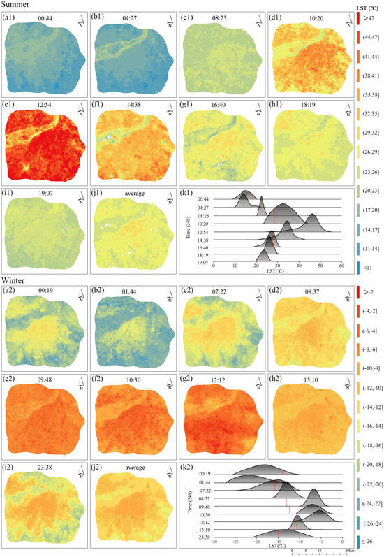
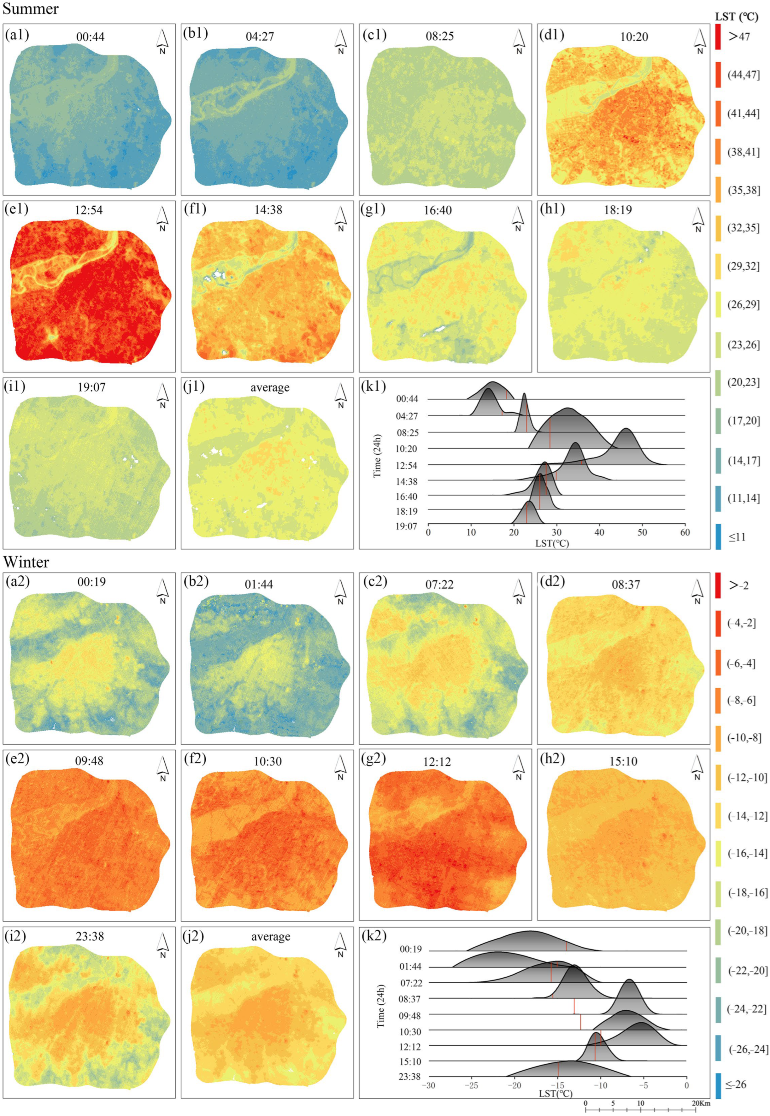
The diurnal variation in LST in summer and winter is shown in Figure 2. LST exhibits distinct diurnal patterns in summer and winter, with urban centers generally warmer than suburban areas. Cumulative analysis reveals that, in summer, the LST reaches its minimum value at 04:27 AM and experiences the fastest increase between 10:20 AM and 12:54 PM, reaching its peak around 12:54 PM before gradually decreasing. During the daytime, LST is notably higher than air temperature, especially around noon, when LST peaks above 50 °C, while air temperature remains significantly lower, indicating rapid surface heating from solar radiation, especially in exposed surfaces and urban areas, where the temperature difference is most pronounced. At night, LST gradually decreases but remains generally higher than air temperature, indicating slower heat release from the surface and more moderate nighttime cooling.

Figure 2. Diurnal variation and spatial pattern of LST in the study area. (a1–j1,a2–j2) show LST at different times of day. (k1,k2) shows the distribution of LST values for all time periods. The red line indicates air temperature, illustrating the difference between surface and air heating throughout the day. The shaded area represents the distribution of LST.

In winter, LST reaches its minimum value at 01:44 AM, with temperatures in some areas dropping below −21 °C. It then gradually increases after sunrise, with the most significant warming occurring between 08:37 AM and 09:48 AM, reaching its peak around 12:12 PM, with temperatures in some areas exceeding −5 °C, before gradually decreasing. At night, LST is noticeably lower than air temperature, indicating faster surface heat loss and a larger temperature drop, leading to an enhanced cooling effect. During the day, LST is slightly higher than air temperature, but the overall temperature difference is smaller, with the average LST fluctuation ranging from −15 °C to −5 °C, indicating a weaker heating effect from solar radiation in winter, with smaller LST fluctuations. Compared to summer, winter LST is less influenced by solar radiation, and nighttime cooling is more pronounced.

3.2. The Nonlinear Influence of Urban Morphological Metrics on LST

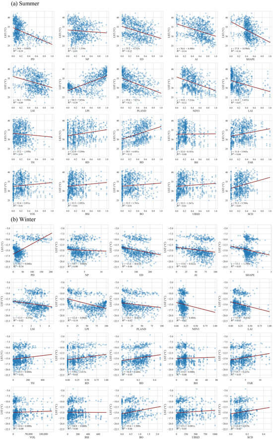
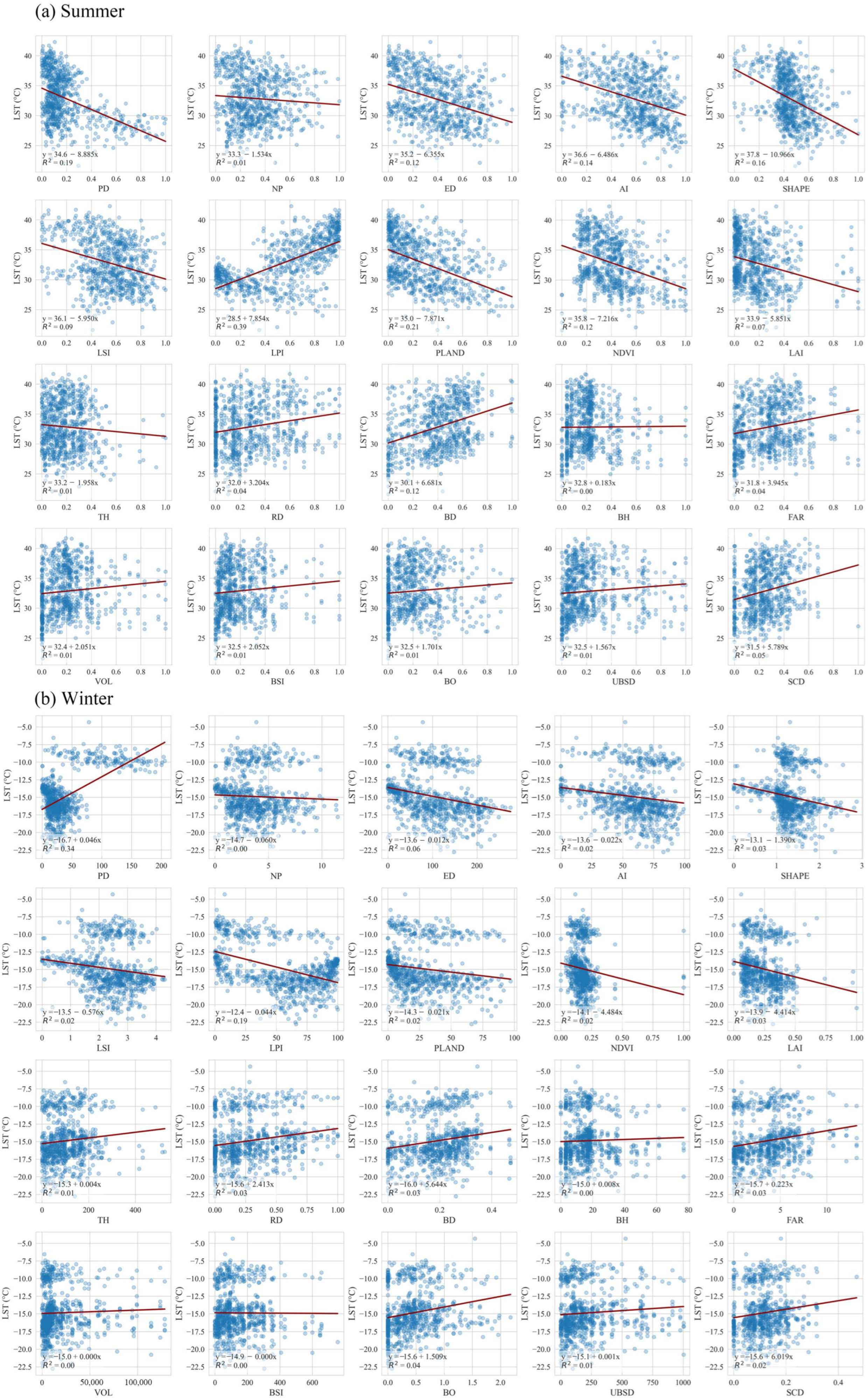
The influence of urban morphological metrics on LST appears generally weak, with most parameters showing little or no linear correlation in either summer or winter. Figure 3 provides an exploratory view of potential linear trends. While some parameters show minor associations with LST, the overall data exhibit considerable scatter. These observations suggest that linear relationships alone may not fully capture the influence of urban morphology on LST, and further research is needed to investigate more complex nonlinear or interactive effects.

Figure 3. Scatter plots and regression lines for urban morphology and summer LST; (b) Scatter plots and regression lines for urban morphology and winterLST. Blue dots represent the observed data points, and the red lines represent the fitted linear regression lines.

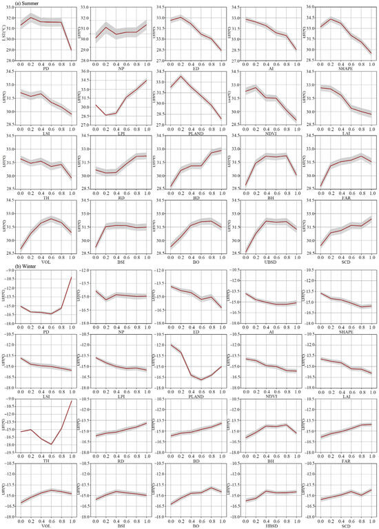
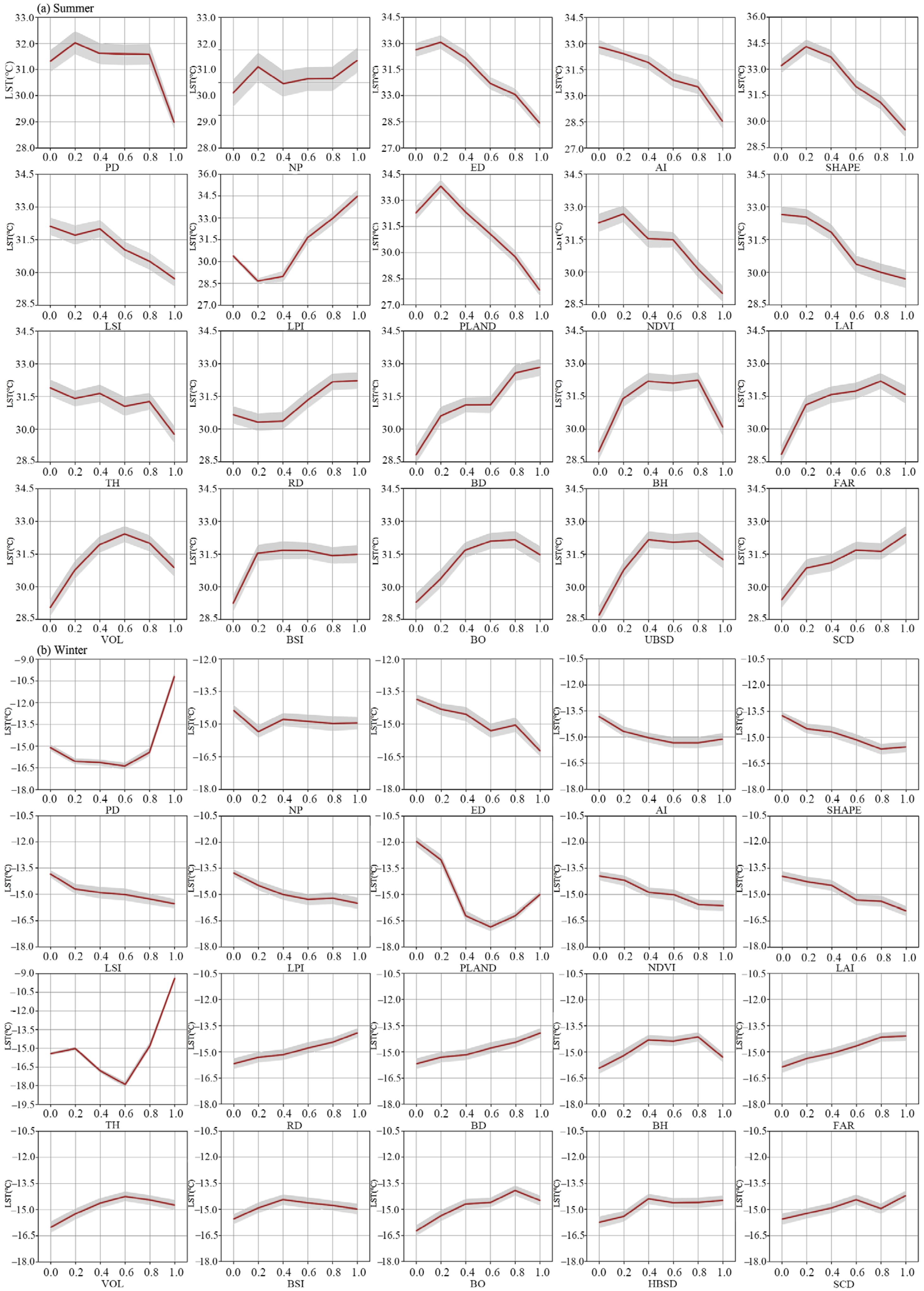
The further nonlinear analysis results, shown in Figure 4, reveal a significant nonlinear relationship between urban morphology and LST. Statistical analysis indicates that, in summer, except for NP and LPI, other landscape pattern indices exhibit a negative influence trend with LST. When RD, BD, and SCD values are high, the urban heat absorption and heat retention effects become more significant. BH, FAR, VOL, BSI, BO, and UBSD show a positive influence on LST in the low-to-medium range, but become negatively correlated with LST at higher values. This may be due to the expansion of buildings and impervious surfaces, which intensifies heat accumulation and retention effects. However, as building height and volume increase further, the shading effect between buildings becomes stronger, reducing solar radiation absorption by the surface and, consequently, lowering LST.

Figure 4. Correlation analysis between 2D and 3D urban morphological metrics and LST. (a) summer and (b) winter. The x-axis shows the values of each urban morphological metric, the y-axis shows LST values, and the lines represent the fitted relationships between each metric and LST. The shaded areas indicate the confidence intervals.

In winter, except for PD, landscape pattern indices exhibit a negative influence trend with LST, but this trend is milder compared to summer. Additionally, TH is negatively correlated with LST at low values and positively correlated at medium-to-high values. This could be because low evergreen shrub crowns block solar radiation from reaching the surface in winter, while taller tree crowns are relatively sparse, allowing more solar radiation to penetrate and reach the surface. RD, BD, and FAR show a positive correlation with LST, and FAR stabilizes at higher values. BH, VOL, BSI, BO, and UMSD exhibit a trend of positive correlation followed by negative correlation with LST. This change may be due to the dominance of heat capacity, shading effects, and heat retention effects at lower and medium values, which increase LST. However, at higher values, shading, reflection, and air flow factors gradually become dominant, leading to a decrease in LST. This suggests that as the number or volume of buildings increases, their contribution to the overall temperature in the area gradually diminishes.

3.3. Relative Importance of Urban Morphology Metrics on Diurnal LST

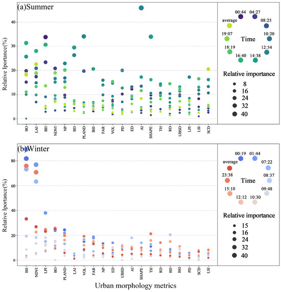
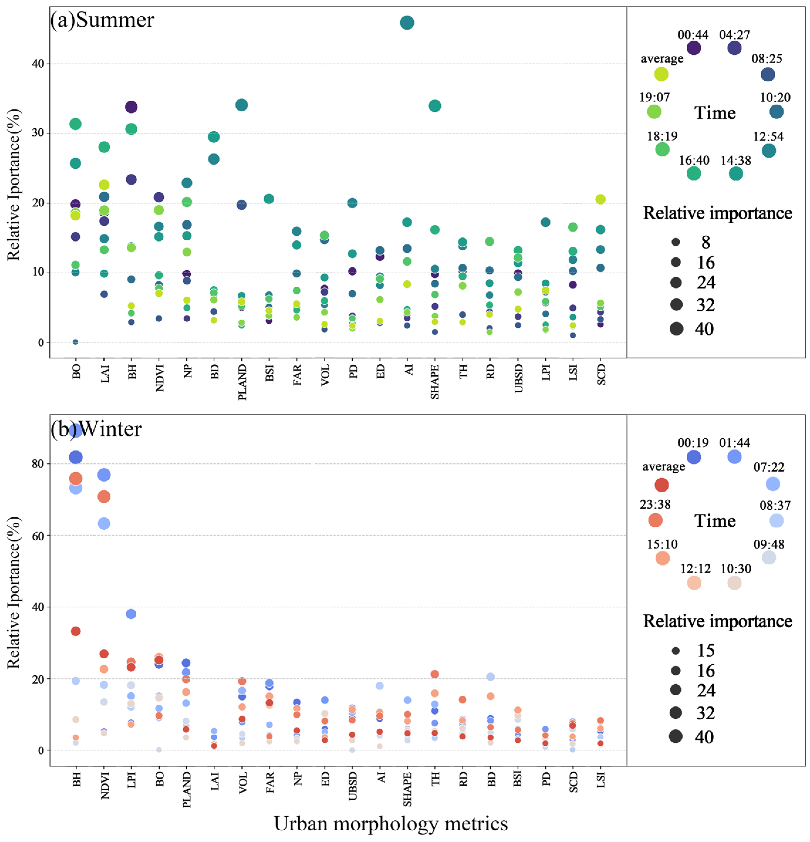
The assessment of the relative importance of urban morphology indicators on daily LST is presented in Figure 5, based on SHAP-derived feature importance rankings from the trained machine learning model. In summer, the top five indicators with the highest impact on daily LST are: BO (16.72%), LAI (16.55%), BH (15.19%), NDVI (13.04%), and NP (12.80%). The relative importance of these indicators fluctuates over time. At 12:54, AI has the highest relative importance, reaching 45.89%. In winter, the top five indicators influencing daily LST are: BH (39.67%), NDVI (33.10%), LPI (15.87%), BO (15.09%), and PLAND (12.68%). Compared to summer, winter LST changes are more heavily influenced by BH and NDVI, suggesting that building height and vegetation indices play a more significant role in winter. Particularly at 01:44, BH’s relative importance reaches 89.24%, indicating its dominant influence on LST during winter nights. Both BO, BH, and NDVI exhibit high relative importance in both summer and winter, indicating that these indicators have a stable influence on LST across seasons.

Figure 5. Relative importance of urban morphology metrics on diurnal LST. The x-axis represents the urban morphology metrics, and the y-axis shows the relative importance (%) of each metric. The color of the points indicates the observation time, including the daily average (average), the size of the points represents the relative importance level, and the position of each point reflects the percentage importance of the corresponding metric at that time. (a) summer, (b) winter.

3.4. The Interactive Effects Between Urban Morphological Parameters

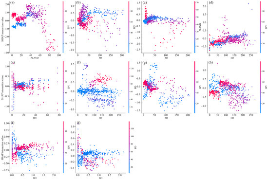
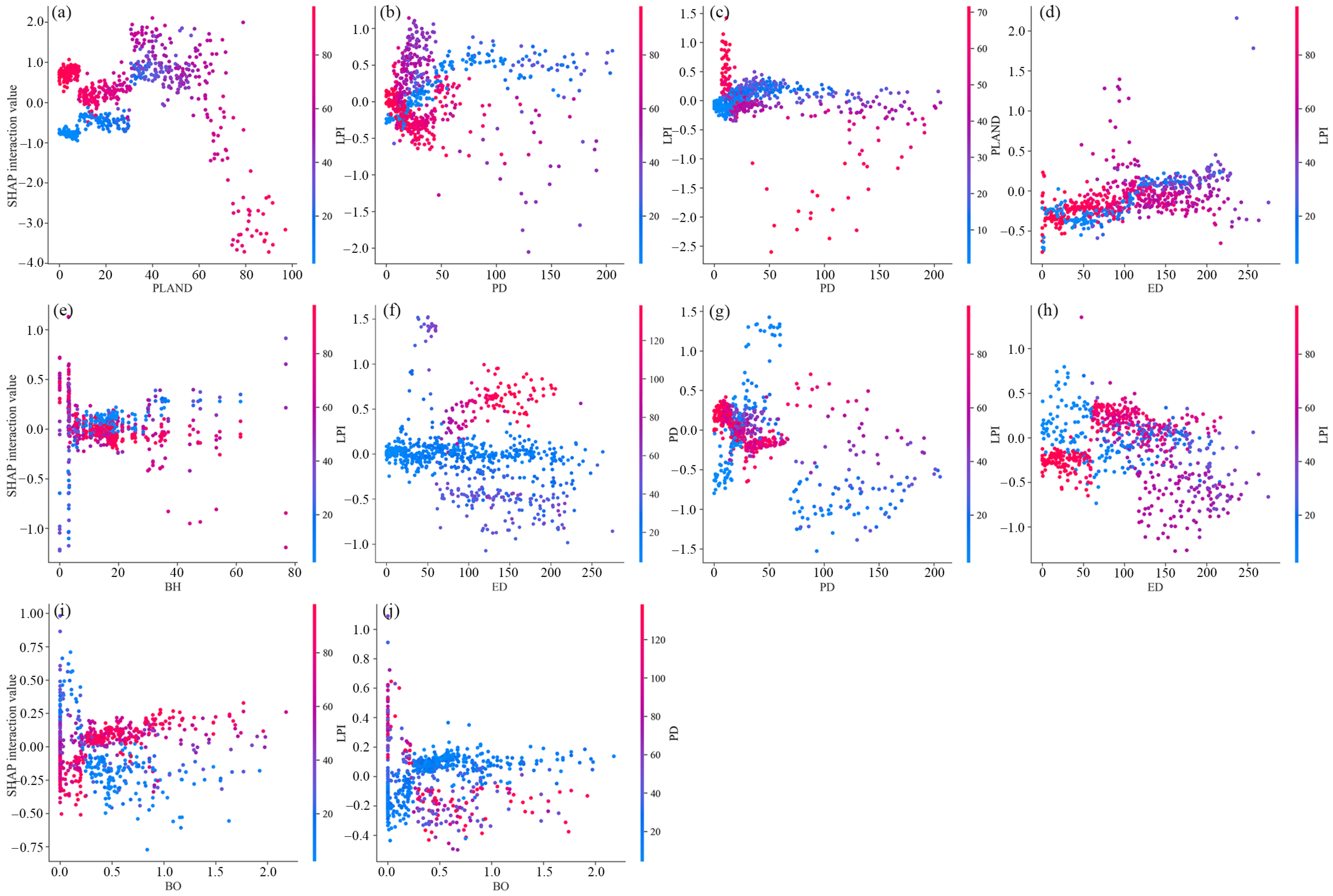
A total of 380 pairwise SHAP interaction plots were generated, and the top 10 strongest interactions were selected to examine how urban morphology metrics jointly influence LST, as shown in Figure 6. The x-axis represents a specific urban morphology parameter, the color bar on the right indicates the urban morphology parameter with the strongest interaction, and the y-axis shows the SHAP interaction values between the two parameters. A SHAP interaction value above 0 reflects a positive interaction, while a value below 0 indicates a negative interaction. When the SHAP interaction value is negative, its absolute value correlates with the strength of the interaction, with larger values leading to a greater reduction in LST.

Figure 6. SHAP interaction effects between urban morphology metrics on LST. The x-axis represents the values of one urban morphology metric, and the y-axis shows the corresponding SHAP interaction values. The color of each point indicates the values of another urban morphology metric. Subplots (a–j) show the interactions between different pairs of urban morphology metrics.

3.4.1. The Effect of Summertime Interactive Effects on LST

In summer, negative interactions are observed among several urban morphology metrics, indicating joint contributions to reductions in LST. For example, PLAND interacts negatively with LPI in ranges such as 0–35 with low LPI (0–20) and 40–100 with high LPI (60–100). Similarly, PD shows negative interactions with LPI across ranges including PD 0–50 with high LPI (80–100) and PD 50–200 with mid LPI (40–60). Other interactions, such as between PD and PLAND or ED and LPI, also exhibit negative effects in certain intervals. Overall, these patterns demonstrate that the strength and direction of interactions vary across parameter values and are nonlinear and condition-dependent.

3.4.2. The Effect of Wintertime Interactive Effects on LST

In winter, negative interactions are observed among ED, PD, LPI, and BO across multiple ranges. For instance, ED interacts negatively with mid-value PD (40–640), while PD shows negative interactions with high LPI (60–100) when PD is 15–70 and with low LPI (0–50) when PD exceeds 70. Interactions involving ED and LPI, as well as BO with PD or LPI, also display negative effects in specific ranges. These results indicate that the interactive influence of urban morphology on LST is nonlinear and context-dependent, with both magnitude and direction of effects varying among parameter combinations.

3.5. Prediction of Seasonal LST

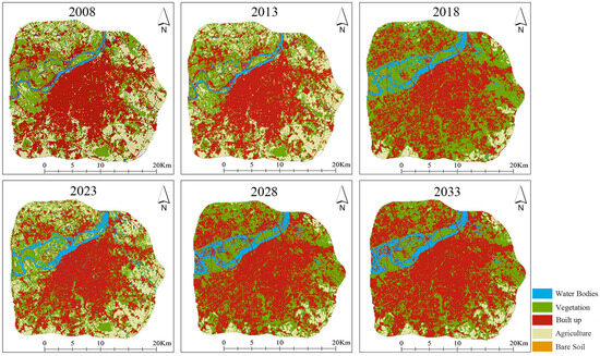
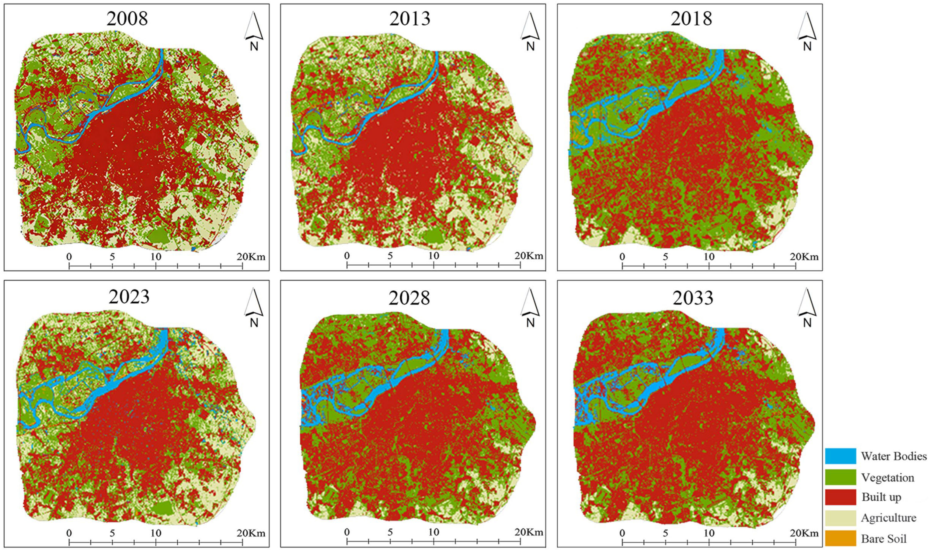
This study is based on land use change information and aims to characterize the potential future evolution of the urban thermal environment. Land use change information predicted using machine learning methods is introduced as a key input factor into the LST prediction model to simulate the spatiotemporal distribution of future land surface temperature. The predicted land use results are shown in Figure 7.

Figure 7. Land use change in the study area.

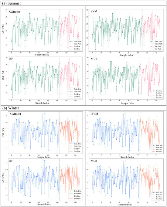
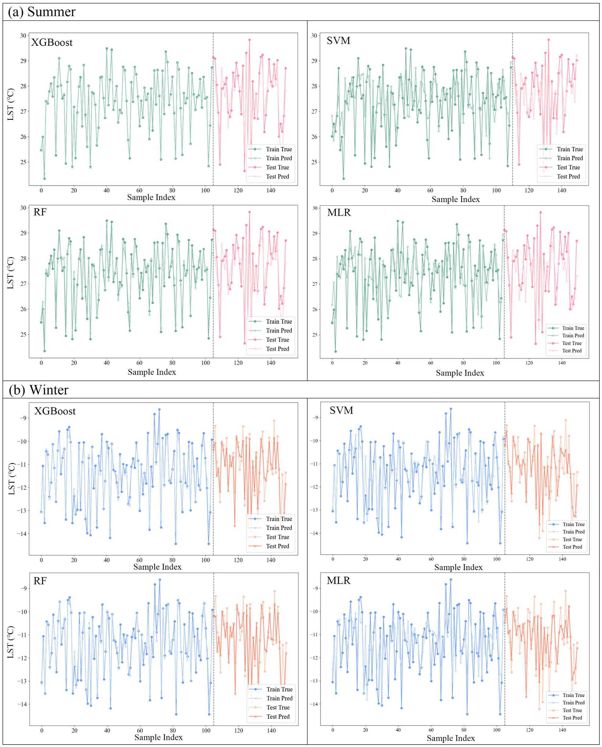
On this basis, the LST prediction performance of five machine learning models under summer and winter conditions was systematically evaluated, as presented in Table 3. Model performance was comprehensively assessed using RMSE, MAPE, and R². The results indicate that XGBoost exhibits the highest prediction accuracy and fitting capability in both seasons, with the lowest error levels and high stability. SVM and RF also demonstrate good predictive performance and reliability, although their overall performance is inferior to that of XGBoost. In contrast, MLR shows relatively weaker predictive capability and fails to adequately capture the nonlinear characteristics of LST and its temporal variation patterns. A comparison between predicted and observed values is shown in Figure 8, where XGBoost exhibits a high degree of consistency in both summer and winter, indicating its effectiveness in simulating the spatiotemporal variations in LST.

Table 3. Performance evaluation of different selected algorithms.

Model	Season	RMSE	MAPE%	R2
XGBoost	Summer	0.60	1.83	0.77
	Winter	0.56	3.89	0.81
SVM	Summer	0.72	2.22	0.70
	Winter	0.68	4.47	0.74
RF	Summer	0.65	1.95	0.74
	Winter	0.61	3.98	0.78
MLR	Summer	0.73	2.20	0.66
	Winter	0.71	4.97	0.71

Figure 8. Comparison of actual LST and predicted LST from different models.

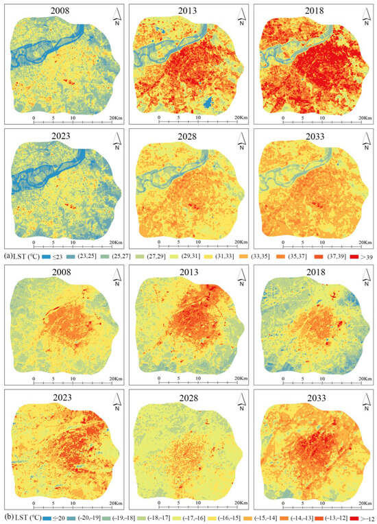
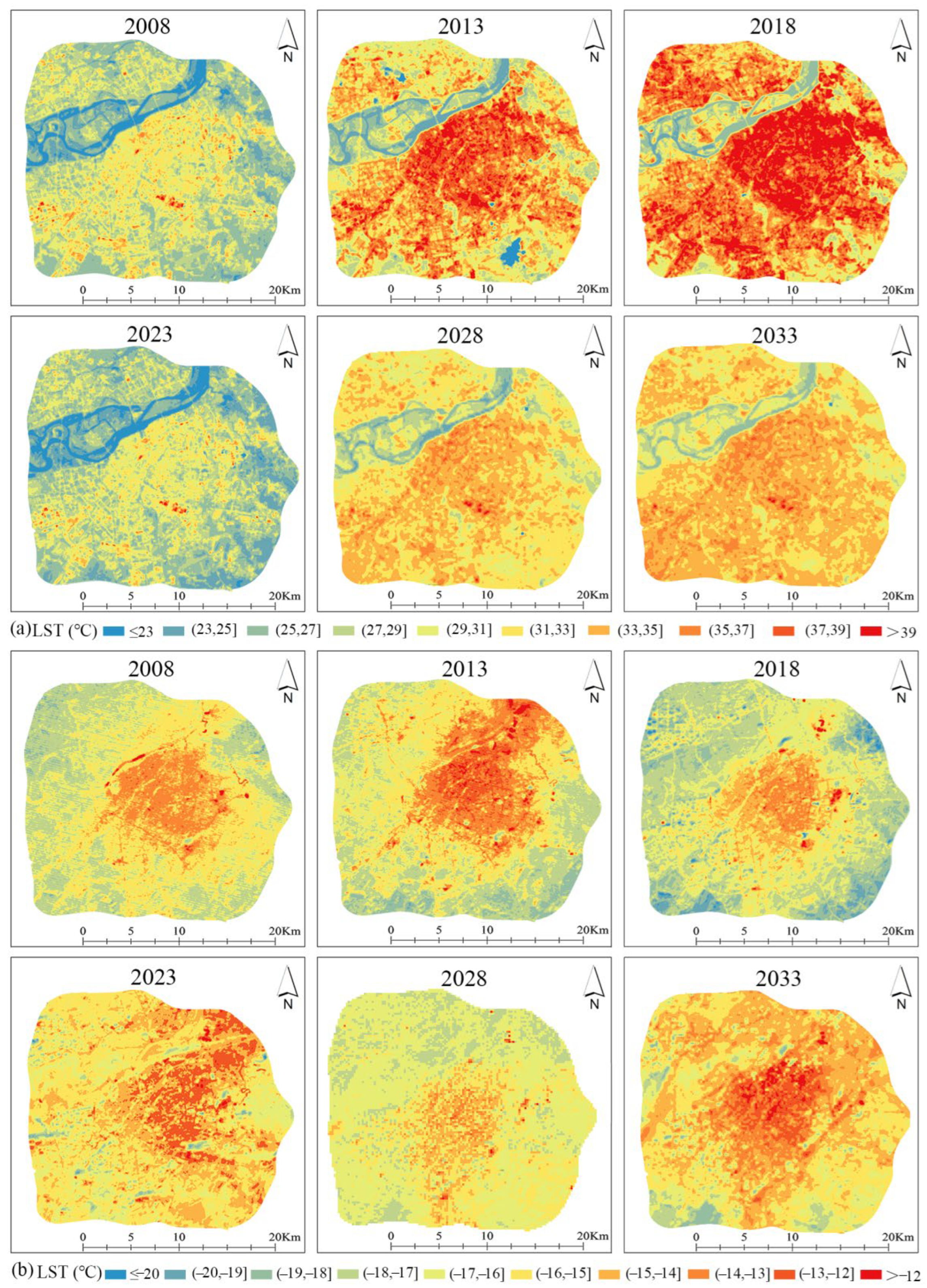
After comparing the prediction performance of five machine learning models, XGBoost was selected for LST prediction analysis. The predicted LST results for the summer and winter of 2028 and 2033 are shown in Figure 9. The results indicate that the area of the highest LST values in the summer of 2028 and 2033 has a relatively small increase, while the area of the highest LST values in winter decreases. Between 2008 and 2033, the area of the highest temperature zone in summer increased by 0.30 km², while the high-temperature area expanded by 45.61 km². In winter, the area of the highest temperature zone decreased by 0.58 km², while the high-temperature area increased by 7.69 km². Overall, from 2008 to 2033, the area of high-temperature zones increased in both summer and winter, while the area of extreme high-temperature zones remained stable. This analysis highlights the significant changes in LST distribution over time, indicating a trend toward higher temperatures in urban areas, particularly in the summer months.

Figure 9. Simulated Summer and Winter LST maps of the study area for years 2028 and 2033.

4. Discussion

4.1. The Effect of 2D and 3D Urban Morphology on LST

Urban morphology is a key factor influencing LST, exhibiting complex nonlinear relationships that vary with season and time of day. Our research further verifies this relationship and reveals a more complex underlying mechanism. The impact of urban morphology on LST exhibits a nonlinear relationship, rather than a simple positive or negative correlation. The influence of urban morphology varies across seasons and times of day. This variation is related to changes in solar radiation, air temperature fluctuations, and differences in surface heat storage and release. This conclusion is consistent with previous research findings [40]. Table 4 summarizes the main findings from related studies.

Table 4. Urban morphology and surface temperature study table.

Research Site	Köppen Climate Zone Classification	Method	Related Conclusions
Chengdu, China (2025) [41]	Cwa	GBRT + SHAP	Impervious surfaces have a profound impact on LST, with vegetation and building configurations playing a particularly significant role during spring and winter nights. BH between 10 and 20 m and densities ranging from 30% to 40% are found to notably raise LST.
Hong Kong, China (2025) [42]	Cfa	ANN + RF	The relationships between urban form and air temperature are predominantly non-linear.
Beijing, China (2024) [43]	Dwa	Correlation Analysis + XGBoost	2D/3D vegetation parameters have the greatest summer cooling effect at 21:00, while SVF impacts minimum nighttime temperature more.
Shenyang, China (2024) [44]	Dwa	Spearman coefficient + BRT	Vegetation contributed to the cooling effect on daytime LST in summer, contributing 29.79%. 3D indicators, such as building height and building density, contributed to diurnal LST.
Guangzhou, China (2024) [45]	Cfa	RF	Vegetation serves as a significant cooling factor in summer, with its patchy and irregular distribution enhancing the cooling effect, particularly in commercial and residential areas.
Hangzhou, China (2023) [46]	Cfa	RF	2D indicators generally exert a stronger influence on LST during warmer seasons, whereas 3D indicators have a more pronounced effect in cooler seasons.

The impact of 2D and 3D urban morphology indicators on LST shows different patterns of influence across seasons and affects the spatial distribution of LST [47]. In both summer and winter, the effects of 2D urban morphology parameters (such as PD and LPI) and 3D urban morphology parameters (such as TH) on LST exhibit significant differences in their mechanisms. In winter, the evaporative cooling effect of green space patches significantly weakens, while bare soil or dead grass, with lower heat capacity, switches from cooling to heat absorption [48]. At the same time, the shading and transpiration cooling effects of trees become ineffective in winter, causing LST to rise further. As the values of BH and other 3D building morphology indicators (such as VOL, BSI, BO, UBSD) increase, the relationship between 3D building morphology indicators and LST shifts from positive to negative, eventually stabilizing as a negative correlation. This phenomenon is consistent with Zhang’s findings [49]. The reason may be that, initially, the increase in building volume enhances heat absorption, but as shading effects and high albedo surfaces increase, heat absorption gradually decreases, leading to surface cooling [50].

The interpretability results from the machine learning model analysis indicate that the importance of 2D and 3D urban morphology parameters on LST exhibits significant diurnal variation. Urban green spaces are identified as key factors in regulating summer LST. AI, PLAND, and SHAPE significantly influence daytime LST, which aligns with previous research findings [51]. Increasing LAI and the amount of green space can enhance the shading effect of trees on impervious surfaces, especially during midday and afternoon periods [52]. Urban green spaces also have an impact on winter nighttime LST. In cases where vegetation has shed its leaves or is sparse, larger areas of bare land promote the dissipation of surface heat by enhancing surface permeability and air circulation, significantly altering LST distribution and variation. Apart from vegetation, 3D urban morphology plays a key role in the diurnal variation in LST. BO has the most significant impact on afternoon LST in both summer and winter. This is because BO regulates heat through the shadow effect and reflection properties of buildings, while BH reduces heat loss due to the larger building volume [53].

In conclusion, a single linear model is inadequate for revealing the complex nonlinear relationship between urban morphology and LST. Nonlinear models have distinct advantages in capturing the multidimensional impact of urban morphology on LST, especially when considering seasonal changes and diurnal temperature variations.

4.2. Interaction Effect of 2Dand 3D Urban Morphology Variables on LST

Our findings suggest that the influence of 2D and 3D urban morphology variables on LST varies across seasons, with building-related metrics and vegetation variables jointly associated with urban thermal patterns. In summer, variables such as BO, LAI, BH, NDVI, and NP appear to have relatively higher contributions, while in winter, BH and NDVI show stronger associations with LST. These patterns may reflect the combined influence of urban structures and vegetation on surface temperatures, although the underlying mechanisms cannot be directly inferred from the model results. Across both seasons, BO, BH, and NDVI tend to be recurrently associated with LST variations, highlighting the dynamic nature of urban thermal processes.

Building on this temporal analysis, SHAP analysis is employed to examine the interactions between urban morphology variables across different seasons. Ten pairs of features with relatively strong interactions are identified and further analyzed for their seasonal and diurnal trends. In summer, negative interactions between building height and green space indicators are associated with lower LST, suggesting that the interaction between building and landscape morphology may be related to urban thermal patterns [54]. Additionally, relatively strong negative contributions to LST are observed under conditions of higher green space coverage and larger patch dominance (e.g., coverage above 60%), indicating that certain landscape configurations are associated with cooling patterns. These patterns may be related to the spatial organization of green spaces and their interaction with built structures [55]. Overall, the results indicate that variations in green space configuration may be associated with differences in LST, although these relationships are better understood as data-driven associations rather than direct causal links.

In winter, interactions between building morphology and landscape features, as well as among different landscape variables, exhibit varying influences on urban surface temperatures [56]. The cooling effects associated with green spaces appear to depend on both the distribution and size of patches, as well as the variability of building heights. In general, larger and more continuous green spaces tend to correspond with relatively lower LST, whereas smaller or more dispersed patches can also contribute to local temperature moderation under certain urban configurations [57]. These observations suggest that the thermal environment is shaped by complex interactions between built structures and landscape elements, with effects that may vary across space and time. Overall, the results suggest that both building and landscape morphology may influence urban thermal conditions during winter.

4.3. Recommendations for Mitigating UHI Effects

Mitigating urban heat requires integrated strategies that optimize both 2D and 3D urban morphology, taking into account seasonal and diurnal variations in LST. In neighborhoods with higher LST, the landscape pattern indicators and BH have a more significant negative impact on LST, further confirming the critical role of green spaces in reducing LST. The findings highlight the potential of optimizing both 2D and 3D urban morphology in mitigating thermal environments. The specific strategies are as follows:

(1) In blocks with high BH, increasing the proportion of the largest green space patches helps reduce summer LST. However, when the proportion of green patches is too low, LST increases. Therefore, when planning and constructing new urban areas, priority should be given to increasing the amount of green space, particularly by expanding the area of the largest green patches to enhance their cooling effects.

(2) In blocks with a large proportion of green patches, increasing the ED and PD can effectively lower summer LST. Thus, when establishing new parks and green spaces, a dispersed layout of green spaces should be adopted, ensuring that the shapes of green patches are regular in order to maximize heat transfer and dissipation effects.

(3) In blocks with high BO, expanding the area of the largest green patches helps store heat during winter, providing a more comfortable outdoor environment for residents in colder regions.

These strategies emphasize the need to carefully consider both the spatial configuration of green spaces and building morphology in urban planning to address both summer and winter thermal challenges.

4.4. Limitations

This study primarily simulates the potential future evolution of the urban thermal environment based on land-use change, under the assumption of a relatively stable urban spatial structure within the selected spatial scale and temporal scope. Accordingly, the analysis focuses on the effects of land-use changes on the spatiotemporal distribution of LST, while the dynamic evolution of urban morphological elements over time is not explicitly considered.

It should be noted that the interaction results presented in this study exhibit some dispersion, reflecting the inherent variability of urban morphology and environmental conditions across different sample blocks. These results should be regarded as preliminary exploratory analyses, providing general trend indications rather than definitive conclusions.

Therefore, over longer temporal scales or broader spatial extents, relying solely on land-use change predictions may be insufficient to fully capture the complex evolution of the urban thermal environment. Future studies could incorporate dynamic changes in urban morphology by integrating land-use transitions with urban form evolution processes, enabling more refined and reliable LST predictions.

5. Conclusions

This study focuses on cities in cold regions and analyzes the daily dynamic characteristics of LST at the block scale. It investigates the nonlinear relationship between LST and both 2D and 3D urban morphological parameters, as well as forecasts future LST changes. The research integrates ECOSTRESS high spatiotemporal resolution LST data, land cover data, and 3D building vector data, extracting 20 urban morphology parameters The XGBoost algorithm and the SHAP framework are employed to quantify the impact of each parameter on LST, with model performance validated using RMSE, MAPE, and R². The main conclusions are as follows:

(1) The influence of urban morphology on LST demonstrates significant seasonal, temporal, and nonlinear characteristics. In the summer, especially at noon and in the afternoon, green space systems have a marked cooling effect; in the winter, particularly at night and in the early morning, BH has a more substantial impact on LST. Some urban morphology parameters (e.g., BH, FAR, VOL, BSI, BO, and UBSD) increase summer LST at low to moderate levels but exhibit cooling effects at higher values. High levels of BH, VOL, BSI, BO, and UBSD contribute to lower winter LST.

(2) In summer, interactions between building and landscape features are associated with variations in urban land surface temperature, with certain combinations of building height and green space configuration showing relatively stronger cooling associations. In winter, the influence of building morphology and green spaces also varies, and both centralized and dispersed green spaces may contribute to temperature regulation.

(3) Among the five predictive models compared, XGBoost outperforms the others, followed by RF, SVM, and MLR. The XGBoost model demonstrates high accuracy and reliability, with RMSE values for summer and winter LST predictions of 0.60 and 0.56, respectively.

This study reveals the nonlinear relationship between urban morphology and LST, emphasizing the importance of rational green space and building layout configurations. This research provides a theoretical foundation for urban heat environment regulation and climate change adaptation in cold region cities, offering insights for future research in these areas.

References

- Akbari, H.; Kolokotsa, D. Three decades of urban heat islands and mitigation technologies research. Energy Build. 2016, 133, 834–842. [Google Scholar] [CrossRef] [Scilit]
- Bansal, P.; Quan, S. Examining temporally varying nonlinear effects of urban form on urban heat island using explainable machine learning: A case of Seoul. Build. Environ. 2024, 247, 110957. [Google Scholar] [CrossRef] [Scilit]
- Guo, A.; Yang, J.; Xiao, X.; Xia, J.; Jin, C.; Li, X. Influences of urban spatial form on urban heat island effects at the community level in China. Sustain. Cities Soc. 2020, 53, 101972. [Google Scholar] [CrossRef] [Scilit]
- Tian, Y.; Zhou, W.; Qian, Y.; Zheng, Z.; Yan, J. The effect of urban 2D and 3D morphology on air temperature in residential neighborhoods. Landsc. Ecol. 2019, 34, 1161–1178. [Google Scholar] [CrossRef] [Scilit]
- Han, J.; Chong, A.; Lim, J.; Ramasamy, S.; Wong, N.; Biljecki, F. Microclimate spatio-temporal prediction using deep learning and land use data. Build. Environ. 2024, 253, 111358. [Google Scholar] [CrossRef] [Scilit]
- Deilami, K.; Kamruzzaman, M.; Liu, Y. Urban heat island effect: A systematic review of spatio-temporal factors, data, methods, and mitigation measures. Int. J. Appl. Earth Obs. 2018, 67, 30–42. [Google Scholar] [CrossRef] [Scilit]
- Zhou, W.; Huang, G.; Cadenasso, M.L. Does spatial configuration matter? Understanding the effects of land cover pattern on land surface temperature in urban landscapes. Landsc. Urban Plan. 2011, 102, 54–63. [Google Scholar] [CrossRef] [Scilit]
- Xu, Y.; Yang, J.; Zheng, Y.; Li, W. Impacts of two-dimensional and three-dimensional urban morphology on urban thermal environments in high-density cities: A case study of Hong Kong. Build. Environ. 2024, 252, 111249. [Google Scholar] [CrossRef] [Scilit]
- Rietze, N.; Assmann, J.J.; Plekhanova, E.; Naegeli, K.; Damm, A.; Maximov, T.C.; Karsanaev, S.V.; Hensgens, G.; Schaepman-Strub, G. Summer drought weakens land surface cooling of tundra vegetation. Environ. Res. Lett. 2024, 19, 044043. [Google Scholar] [CrossRef] [Scilit]
- Gao, J.; Gong, J.; Yang, J.; Li, J.; Li, S. Measuring spatial connectivity between patches of the heat source and sink (SCSS): A new index to quantify the heterogeneity impacts of landscape patterns on land surface temperature. Landsc. Urban Plan. 2022, 217, 104260. [Google Scholar] [CrossRef] [Scilit]
- Seddon, N.; Chausson, A.; Berry, P.; Girardin, C.A.; Smith, A.; Turner, B. Understanding the value and limits of nature-based solutions to climate change and other global challenges. Philos. Trans. R. Soc. Lond. B Biol. Sci. 2020, 375, 20190120. [Google Scholar] [CrossRef] [Scilit] [PubMed]
- Berger, C.; Rosentreter, J.; Voltersen, M.; Baumgart, C.; Schmullius, C.; Hese, S. Spatiotemporal analysis of the relationship between 2D/3D urban site characteristics and land surface temperature. Remote Sens. Environ. 2017, 193, 225–243. [Google Scholar] [CrossRef] [Scilit]
- Wu, W.; Yu, Z.; Ma, J.; Zhao, B. Quantifying the influence of 2D and 3D urban morphology on the thermal environment across climatic zones. Landsc. Urban Plan. 2022, 226, 104499. [Google Scholar] [CrossRef] [Scilit]
- Weng, Q.; Lu, D.; Schubring, J. Estimation of land surface temperature–vegetation abundance relationship for urban heat island studies. Remote Sens. Environ. 2004, 89, 467–483. [Google Scholar] [CrossRef] [Scilit]
- Kamaraj, N.P.; Shekhar, S.; Sivashankari, V.; Balasubramani, K.; Prasad, K.A. Detecting heat-inducing urban built-up surface material with multi remote sensing datasets using reflectance and emission spectroscopy. Remote Sens. Environ. 2021, 264, 112591. [Google Scholar] [CrossRef] [Scilit]
- Chang, Y.; Xiao, J.; Li, X.; Middel, A.; Zhang, Y.; Gu, Z.; Wu, Y.; He, S. Exploring diurnal thermal variations in urban local climate zones with ECOSTRESS land surface temperature data. Remote Sens. Environ. 2021, 263, 112544. [Google Scholar] [CrossRef] [Scilit]
- Yuan, B.; Zhou, L.; Hu, F.; Zhang, Q. Diurnal dynamics of heat exposure in Xi’an: A perspective from local climate zone. Build. Environ. 2022, 222, 109400. [Google Scholar] [CrossRef] [Scilit]
- Hamberg, L.J.; Fisher, J.B.; Ruppert, J.L.; Tureček, J.; Rosen, D.H.; James, P.M. Assessing and modeling diurnal temperature buffering and evapotranspiration dynamics in forest restoration using ECOSTRESS thermal imaging. Remote Sens. Environ. 2022, 280, 113178. [Google Scholar] [CrossRef] [Scilit]
- Li, W.; Cao, Q.; Lang, K.; Wu, J. Linking potential heat source and sink to urban heat island: Heterogeneous effects of landscape pattern on land surface temperature. Sci. Total Environ. 2017, 586, 457–465. [Google Scholar] [CrossRef] [Scilit]
- Zhang, J.; Li, Z.; Wei, Y.; Hu, D. The impact of the building morphology on microclimate and thermal comfort—A case study in Beijing. Build. Environ. 2022, 223, 109469. [Google Scholar] [CrossRef] [Scilit]
- Wu, Y.; Hou, H.; Wang, R.; Murayama, Y.; Wang, L.; Hu, T. Effects of landscape patterns on the morphological evolution of surface urban heat island in Hangzhou during 2000–2020. Sustain. Cities Soc. 2022, 79, 103717. [Google Scholar] [CrossRef] [Scilit]
- Mehrotra, S.; Bardhan, R.; Ramamritham, K. Urban form as policy variable for climate-sensitive area planning under heterogeneity: A geographically weighted regression approach. Area Dev. Policy 2020, 5, 167–188. [Google Scholar] [CrossRef] [Scilit]
- Aslam, B.; Maqsoom, A.; Khalid, N.; Ullah, F.; Sepasgozarilal, S. Urban overheating assessment through prediction of surface temperatures: A case study of Karachi, Pakistan. ISPRS Int. J. Geo-Inf. 2021, 10, 539. [Google Scholar] [CrossRef] [Scilit]
- Mohammad, P.; Goswami, A.; Chauhan, S.; Nayak, S. Machine learning algorithm based prediction of land use land cover and land surface temperature changes to characterize the surface urban heat island phenomena over Ahmedabad city, India. Urban Clim. 2022, 42, 101116. [Google Scholar] [CrossRef] [Scilit]
- Jabeur, S.B.; Mefteh-Wali, S.; Viviani, J.L. Forecasting gold price with the XGBoost algorithm and SHAP interaction values. Ann. Oper. Res. 2024, 334, 679–699. [Google Scholar] [CrossRef] [Scilit]
- Tsai, C.; Chen, Y.; Peña, A.; Paniagua, G. A visiting sequence recommendation framework: Enhanced by dynamic landmark and stay time. Expert Syst. Appl. 2023, 230, 120662. [Google Scholar] [CrossRef] [Scilit]
- Ge, J.; Meng, B.; Liang, T.; Feng, Q.; Gao, J.; Yang, S.; Huang, X.; Xie, H. Modeling alpine grassland cover based on MODIS data and support vector machine regression in the headwater region of the Huanghe River, China. Remote Sens. Environ. 2018, 218, 162–173. [Google Scholar] [CrossRef] [Scilit]
- Ullah, S.; Qiao, X.; Tariq, A. Impact assessment of planned and unplanned urbanization on land surface temperature in Afghanistan using machine learning algorithms: A path toward sustainability. Sci. Rep. 2025, 15, 3092. [Google Scholar] [CrossRef] [Scilit]
- Zhang, J.; Cui, P.; Song, H. Impact of urban morphology on outdoor air temperature and microclimate optimization strategy base on Pareto optimality in Northeast China. Build. Environ. 2020, 180, 107035. [Google Scholar] [CrossRef] [Scilit]
- Cui, P.; Jiang, J.; Zhang, J.; Wang, L. Effect of street design on UHI and energy consumption based on vegetation and street aspect ratio: Taking Harbin as an example. Sustain. Cities Soc. 2023, 92, 104484. [Google Scholar] [CrossRef] [Scilit]
- He, Y.; Abel, T.; Wong, N. A parametric study of angular road patterns on pedestrian ventilation in high-density urban areas. Build. Environ. 2019, 151, 251–267. [Google Scholar] [CrossRef] [Scilit]
- Welegedara, N.P.Y.; Agrawal, S.K.; Lotfi, G. Exploring spatiotemporal changes of the urban heat island effect in high-latitude cities at a neighbourhood level: A case of Edmonton, Canada. Sustain. Cities Soc. 2023, 90, 104403. [Google Scholar] [CrossRef] [Scilit]
- Li, H.; Li, Y.; Wan, T.; Wang, Z.; Gao, M.; Shen, H. Quantifying 3D building form effects on urban land surface temperature and modeling seasonal correlation patterns. Build. Environ. 2021, 204, 108132. [Google Scholar] [CrossRef] [Scilit]
- Liu, Y.; Li, Q.; Yang, L.; Mu, K.; Zhang, M.; Liu, J. Urban heat island effects of various urban morphologies under regional climate conditions. Sci. Total Environ. 2020, 743, 140589. [Google Scholar] [CrossRef] [Scilit]
- Hulley, G.C.; Gottsche, F.M.; Rivera, G.; Hook, S.J.; Freepartner, R.J.; Martin, M.A.; Cawse-Nicholson, K.; Johnson, W.R. Validation and quality assessment of the ECOSTRESS level-2 land surface temperature and emissivity product. IEEE Trans. Geosci. Remote Sens. 2021, 60, 5000523. [Google Scholar] [CrossRef] [Scilit]
- Tan, W.; Wei, C.; Lu, Y.; Xue, D. Reconstruction of all-weather daytime and nighttime MODIS Aqua–Terra land surface temperature products using an XGBoost approach. Remote Sens. 2021, 13, 4723. [Google Scholar] [CrossRef] [Scilit]
- Liu, F.; Wang, X.; Sun, F.; Wang, H.; Wu, L.; Zhang, X.; Liu, W.; Che, H. Correction of overestimation in observed land surface temperatures based on machine learning models. J. Clim. 2022, 35, 5359–5377. [Google Scholar] [CrossRef] [Scilit]
- Lundberg, S. A unified approach to interpreting model predictions. arXiv 2017, arXiv:1705.07874. [Google Scholar] [CrossRef] [Scilit]
- Lundberg, S.M.; Erion, G.G.; Lee, S.I. Consistent individualized feature attribution for tree ensembles. arXiv 2018, arXiv:1802.03888. [Google Scholar]
- Wang, Z.; Zhou, R.; Yu, Y. The impact of urban morphology on land surface temperature under seasonal and diurnal variations: Marginal and interaction effects. Build. Environ. 2025, 272, 112673. [Google Scholar] [CrossRef] [Scilit]
- Wang, Z.; Zhou, R.; Rui, J.; Yu, Y. Revealing the impact of urban spatial morphology on land surface temperature in plain and plateau cities using explainable machine learning. Sustain. Cities Soc. 2025, 118, 106046. [Google Scholar] [CrossRef] [Scilit]
- Tian, L.; Hao, T.; He, X.; Chan, I.; Niu, J.; Chan, P.; Ng, W.; Huang, J. Examining the non-linear relationship between urban form and air temperature at street level: A case of Hong Kong. Build. Environ. 2024, 264, 111884. [Google Scholar] [CrossRef] [Scilit]
- He, W.; Cao, S.; Du, M.; Meng, X.; Yang, Z.; Yang, Y. The effect of urban form parameters on annual and diurnal cycles of land surface temperature with 30-meter hourly resolution. Sustain. Cities Soc. 2024, 115, 105806. [Google Scholar] [CrossRef] [Scilit]
- Zhang, Q.; Yang, J.; Ma, X.; Xin, J.; Ren, J.; Yu, W.; Xiao, X.; Xia, J. Influence of 2D/3D urban morphology on diurnal land surface temperature from the perspective of functional zones. IEEE J. Sel. Top. Appl. Earth Obs. Remote Sens. 2024, 17, 17036–17051. [Google Scholar] [CrossRef] [Scilit]
- Liu, Y.; Zhang, W.; Liu, W.; Tan, Z.; Hu, S.; Ao, Z.; Li, J.; Xing, H. Exploring the seasonal effects of urban morphology on land surface temperature in urban functional zones. Sustain. Cities Soc. 2024, 103, 105268. [Google Scholar] [CrossRef] [Scilit]
- Han, S.; Hou, H.; Estoque, R.C.; Zheng, Y.; Shen, C.; Murayama, Y.; Pan, J.; Wang, B.; Hu, T. Seasonal effects of urban morphology on land surface temperature in a three-dimensional perspective: A case study in Hangzhou, China. Build. Environ. 2023, 228, 109913. [Google Scholar] [CrossRef] [Scilit]
- Guo, L.; Du, S.; Sun, W.; Fan, D.; Wu, Y. Multi-scale impact of urban building function and 2D/3D morphology on urban heat island effect: A case study in Shanghai, China. Energy Build. 2025, 338, 115719. [Google Scholar] [CrossRef] [Scilit]
- Chen, H.; Liu, R.; Zhang, Y. The impact of vegetation canopy on the outdoor thermal environment in cold winter and spring. Sustainability 2023, 15, 12818. [Google Scholar] [CrossRef] [Scilit]
- Zhang, Z.; Luan, W.; Yang, J.; Guo, A.; Su, M.; Tian, C. The influences of 2D/3D urban morphology on land surface temperature at the block scale in Chinese megacities. Urban Clim. 2023, 49, 101553. [Google Scholar] [CrossRef] [Scilit]
- Yang, C.; Zhu, W.; Sun, J.; Xu, X.; Wang, R.; Lu, Y.; Zhou, W. Assessing the effects of 2D/3D urban morphology on the 3D urban thermal environment by using multi-source remote sensing data and UAV measurements: A case study of the snow-climate city of Changchun, China. J. Clean. Prod. 2021, 321, 128956. [Google Scholar] [CrossRef] [Scilit]
- Li, J.; Song, C.; Cao, L.; Zhu, F.; Meng, X.; Wu, J. Impacts of landscape structure on surface urban heat islands: A case study of Shanghai, China. Remote Sens. Environ. 2011, 115, 3249–3263. [Google Scholar] [CrossRef] [Scilit]
- Cui, Y.Y.; De Foy, B. Seasonal variations of the urban heat island at the surface and the near-surface and reductions due to urban vegetation in Mexico City. J. Appl. Meteorol. Clim. 2012, 51, 855–868. [Google Scholar] [CrossRef] [Scilit]
- Loughner, C.P.; Allen, D.J.; Zhang, D.L.; Pickering, K.E.; Dickerson, R.R.; Landry, L. Roles of urban tree canopy and buildings in urban heat island effects: Parameterization and preliminary results. J. Appl. Meteorol. Climatol. 2012, 51, 1775–1793. [Google Scholar] [CrossRef] [Scilit]
- Yang, F.; Lau, S.S.Y.; Qian, F. Summertime heat island intensities in three high-rise housing quarters in inner-city Shanghai China: Building layout, density and greenery. Build. Environ. 2010, 45, 115–134. [Google Scholar] [CrossRef] [Scilit]
- Wu, Y.; Patuano, A.; Mashhoodi, B.; Lenzholzer, S.; Acred, A.; Zertuche, L.N. How small green spaces cool urban neighbourhoods: Optimising distribution, size and shape. Landsc. Urban Plan. 2025, 253, 105224. [Google Scholar] [CrossRef] [Scilit]
- Wang, Y.; Ren, Y. Cooling efficiency of urban green spaces across functional zones: Mitigating heat island effects through spatial configuration. Sustainability 2025, 17, 2275. [Google Scholar] [CrossRef] [Scilit]
- Bao, T.; Li, X.; Zhang, J.; Zhang, Y.; Tian, S. Assessing the distribution of urban green spaces and its anisotropic cooling distance on urban heat island pattern in Baotou, China. ISPRS Int. J. Geo-Inf. 2016, 5, 12. [Google Scholar] [CrossRef] [Scilit]
Disclaimer/Publisher’s Note: The statements, opinions and data contained in all publications are solely those of the individual author(s) and contributor(s) and not of MDPI and/or the editor(s). MDPI and/or the editor(s) disclaim responsibility for any injury to people or property resulting from any ideas, methods, instructions or products referred to in the content. |
© 2026 by the authors. Licensee MDPI, Basel, Switzerland. This article is an open access article distributed under the terms and conditions of the Creative Commons Attribution (CC BY) license.