


Abstract
To enhance the resilience of urban road networks under frequent recurrent disturbances such as morning peak commuting congestion, this study develops a dynamic resilience assessment framework from the perspective of land-use mix. The model evaluates network resilience by quantifying performance evolution and recovery capacity during the morning peak from both road segment and node dimensions, using land-use mix entropy to characterize functional complexity. The compounded effects of tidal commuting directions and land-use mix are further investigated. Results indicate clear heterogeneity in degradation and recovery trajectories across different land-use mix levels: segments and nodes in high land-use mix areas exhibit more pronounced performance deterioration and delayed recovery. When high land-use mix areas spatially overlap with predominant commuting directions, performance degradation is further amplified and recovery at the end of the morning peak remains lower, revealing critical resilience weaknesses. Accordingly, a land-use mix-oriented targeted optimization strategy is proposed, which enhances system-level resilience by prioritizing capacity improvements on high land-use mix segments. Simulation results show that the proposed strategy increases the network resilience value by 9.46% compared with the baseline scenario, achieving an improvement 2.3 times that of a random capacity expansion strategy. This study provides quantitative evidence for the linkage between land-use mix and dynamic road-network resilience and offers a spatially informed framework for resilience enhancement under recurrent disturbances.
1. Introduction
Urban transportation networks constitute critical infrastructure supporting commuting and urban functioning. Network resilience refers to its capacity to maintain functionality, adapt to changes, and recover rapidly during disruptive events. It is a crucial issue for ensuring sustainable operation of urban transportation systems [1]. With climate change and rising travel demand, robust operation and fast recovery under multiple disturbance sources have become a key concern in transport governance and planning.
In recent years, research on transportation resilience has primarily focused on extreme events [2,3,4,5], such as natural disasters [6,7,8,9], terrorist attacks, and system failures that cause structural damage and functional interruptions to road networks [10,11,12,13,14], with relatively well-developed theoretical and methodological frameworks. A microscopic-simulation-based framework (Simulation of Urban Mobility, SUMO) is proposed to quantify both structural features and functional performance changes across emergency scenarios [15]. Spatial patterns of hazard impacts were incorporated, including hazard intensity and spatial distribution, to track resilience evolution [7]. An indicator-based assessment was developed using origin–destination (OD) datasets and evaluates potential shifts from motorized modes to active modes under disruptions [16]. Crowdsourced data have been applied to assess how rainstorm intensity and demand variation jointly affect resilience [17]. Cascading-failure simulations based on nonlinear load-capacity assumptions further show how modeling choices can alter resilience outcomes [18]. However, research remains relatively underdeveloped regarding high-frequency recurrent disturbances, such as gradual and periodic performance degradation of road networks caused by morning and evening commuting congestion [19]. GPS-based analyses further suggest that peak-period demand fluctuations and weather-related traffic changes can substantially alter network operating states [20]. Although such recurrent disturbances do not cause structural damage, their high frequency and long duration constrain road network service capacity, significantly impacting urban transportation efficiency and residents’ travel experience [21,22]. Understanding dynamic response under recurrent disturbances is therefore important. Scenario-consistent assessment and optimization frameworks are also needed.
Among resilience assessment metrics, various indicators based on complex network theory are extensively employed to quantify road network structural characteristics [23], such as betweenness centrality [24] and node degree [25]. While these indicators effectively characterize static structural features of road networks, they struggle to reflect time-varying traffic flow characteristics and dynamic performance changes under disturbances [26]. To address this limitation, some studies have adopted dynamic performance indicators to assess road network functional status during disturbances, including travel time [2,27], travel flow [28,29,30], and generalized travel cost [31]. Multidimensional quantitative indicators provide a crucial methodological foundation for research on transportation system resilience. To capture degradation and recovery processes, dynamic network vulnerability frameworks have also been introduced [32]. Typical approaches include percolation-based representations [33], stochastic capacity-loss models [34], and simulation methods coupled with dynamic user equilibrium (DUE) [35]. These methods can represent flow redistribution and performance evolution over time. Such methods highlight coupling among network topology, capacity changes, and traveler behavior. Their mechanistic explanations primarily address network responses under pre-specified demand. Morning peak congestion differs in nature. It is a demand-driven recurrent disturbance. Network stress largely comes from rapid, time-varying demand concentration. Demand organization in space and time is closely associated with land-use patterns and functional layout.
Meanwhile, land-use mix intensity serves as a key indicator for characterizing urban spatial functional complexity and potentially influences road network resilience by reshaping spatiotemporal distribution of travel demand [36]. Built-environment research provides a classic theoretical anchor. A 3D framework was proposed covering density, diversity, and design, and identified land-use diversity as an important determinant of travel demand [37]. Ewing and Cervero further synthesize extensive empirical evidence through meta-analysis and confirm stable associations between built-environment attributes [38], including land-use diversity, and travel behavior. In addition, research indicated that incorporating land use patterns into resilience analysis can provide new perspectives for understanding system resilience characteristics [39]. Researchers found that land use significantly influences road network load patterns by reshaping spatial distribution of travel demand [40]. Therefore, integrating land-use factors into a dynamic resilience framework helps clarify links between land-use pattern and resilience degradation.
Under extreme disturbance scenarios, land-use mix intensity exerts relatively limited impact on traffic flow compared to capacity loss caused by physical damage. However, during morning peak, the root cause of large passenger flow disturbance lies not in physical damage but in high spatiotemporal concentration of travel demand [20]. Its spatial and temporal distribution shows strong association with land-use structure and functional layout [41]. High land-use mix areas, such as zones containing multiple different land-use types like schools and hospitals simultaneously, tend to generate multi-directional and continuous traffic demands, making associated road segments more susceptible to becoming traffic bottlenecks. Additionally, non-commuting demands in high-mix intensity areas, such as medical visits, demonstrate persistent and all-day characteristics. Even after commuting peak hours, these areas maintain high traffic attraction, making them more prone to persistent congestion and greater pressure during recovery phases. Notably, morning peak commuting traffic exhibits distinct tidal directionality. When high land-use mix intensity areas spatially overlap with predominant commuting directions, multi-purpose traffic flows generated in these areas and main commuting flows create superposition effects that may further amplify supply–demand imbalances. In a demand-driven morning peak setting, spatial organization of trip generation and attraction, together with tidal commuting, makes land-use structure more influential on system performance. Although this phenomenon has attracted attention, research that systematically integrates land-use mix intensity with directional characteristics into dynamic resilience assessment models remains relatively scarce. Quantitative evidence also remains limited, especially work that links mix-driven demand-organization differences to observable degradation trajectories and recovery differences within a dynamic resilience framework.
Road network resilience is shaped by multiple factors, including demand structure and intensity, network supply such as road class and lane provision, management and enforcement such as curb parking and pick-up or drop-off control, and external conditions such as weather, crashes, construction, and unexpected incidents. These factors jointly affect resilience performance under disturbances. Therefore, this paper firstly constructs a dynamic resilience assessment model for road networks that integrates land-use mix intensity. Secondly, using the Xi’an urban road network as a case study, it examines performance evolution and resilience differences of road segments and nodes across mix levels, and analyzes superposition effects between land-use mix and tidal commuting direction. Finally, a spatial resilience optimization strategy guided by land-use mix intensity is proposed, with simulation results verifying its superiority over a random strategy. This research provides both theoretical foundation and decision support for enhancing urban road network resilience against recurrent disturbances.
2. Materials and Methods
2.1. Qualitative Description of Road Network Resilience
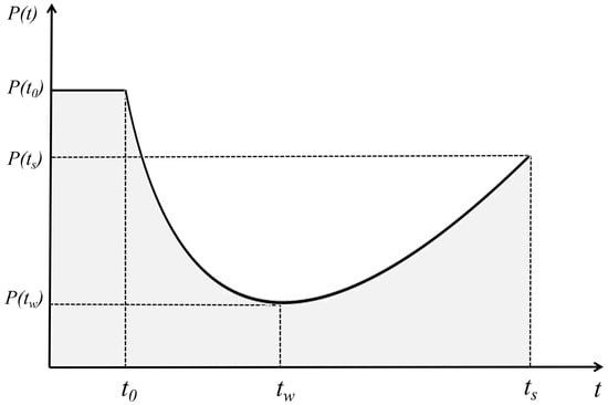
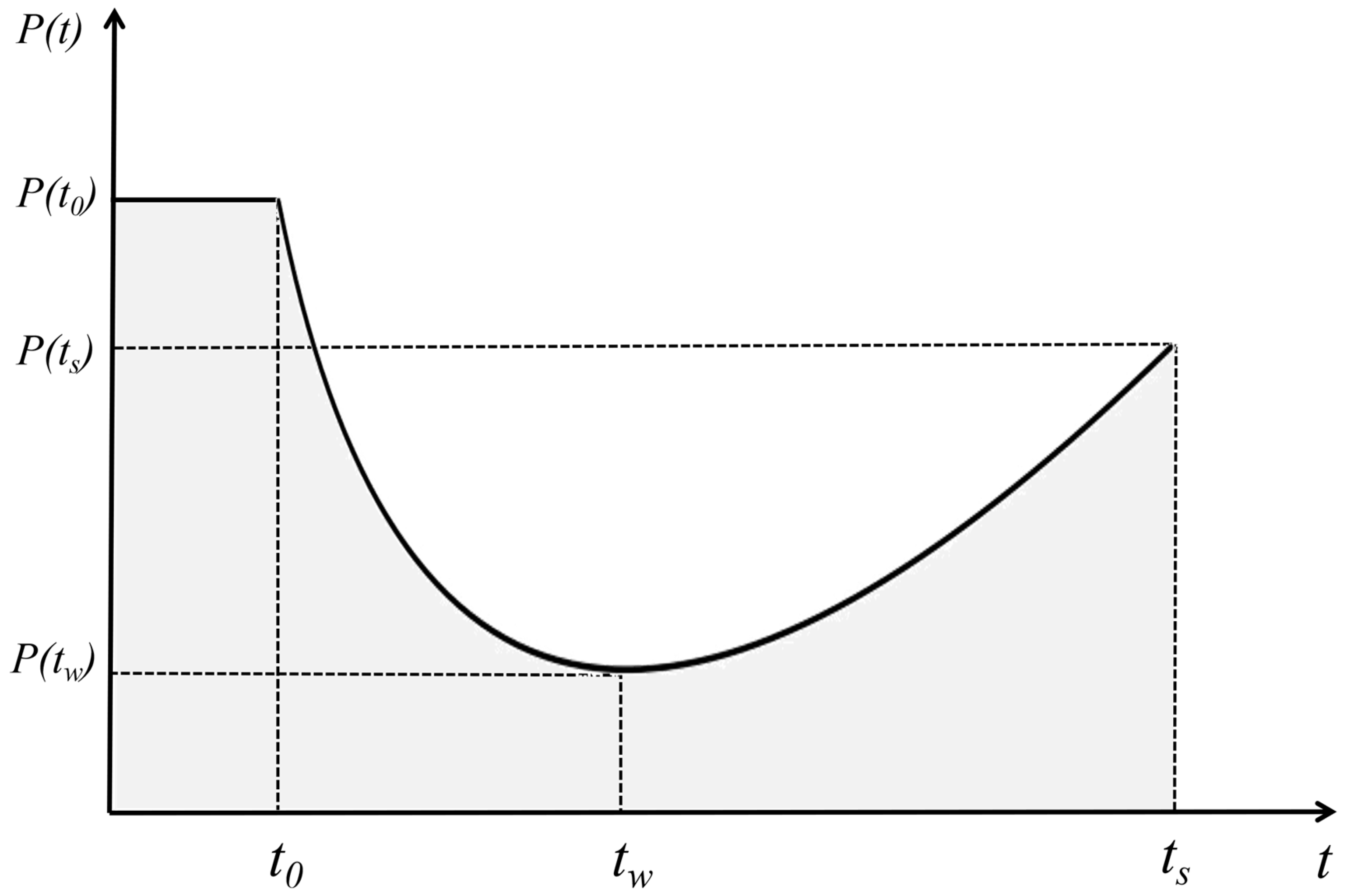
Figure 1 depicts performance evolution of an urban road network under a disruptive event. Time denotes onset of disturbance. Time denotes the moment when system performance reaches its minimum. Time denotes the moment when performance recovers to a certain level and the system enters a new steady state. Corresponding performance values at these times are , , and . Based on this representation, performance evolution under disturbance can be decomposed into two canonical phases: a disturbance-resistance phase from to during which performance degrades as the system resists disturbance. A recovery phase from to , during which performance rebounds toward a post-disturbance steady state.
Figure 1.
Illustration of road network resilience.
Resilience is commonly understood through two core dimensions. Firstly, resistance capacity is reflected by magnitude of performance loss, . Second, recovery capacity is reflected by recovery speed and final recovery level, represented by after disturbance [42]. In this view, overall resilience is associated with how well performance is maintained throughout an entire disruption–recovery cycle. Accordingly, resilience triangle theory is widely adopted to quantify resilience by relative area under a performance curve [43]. Resilience can be computed using Equation (1).
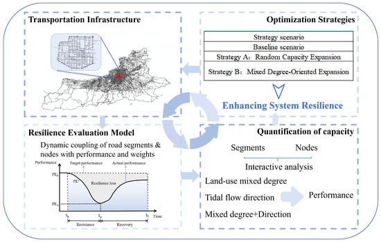
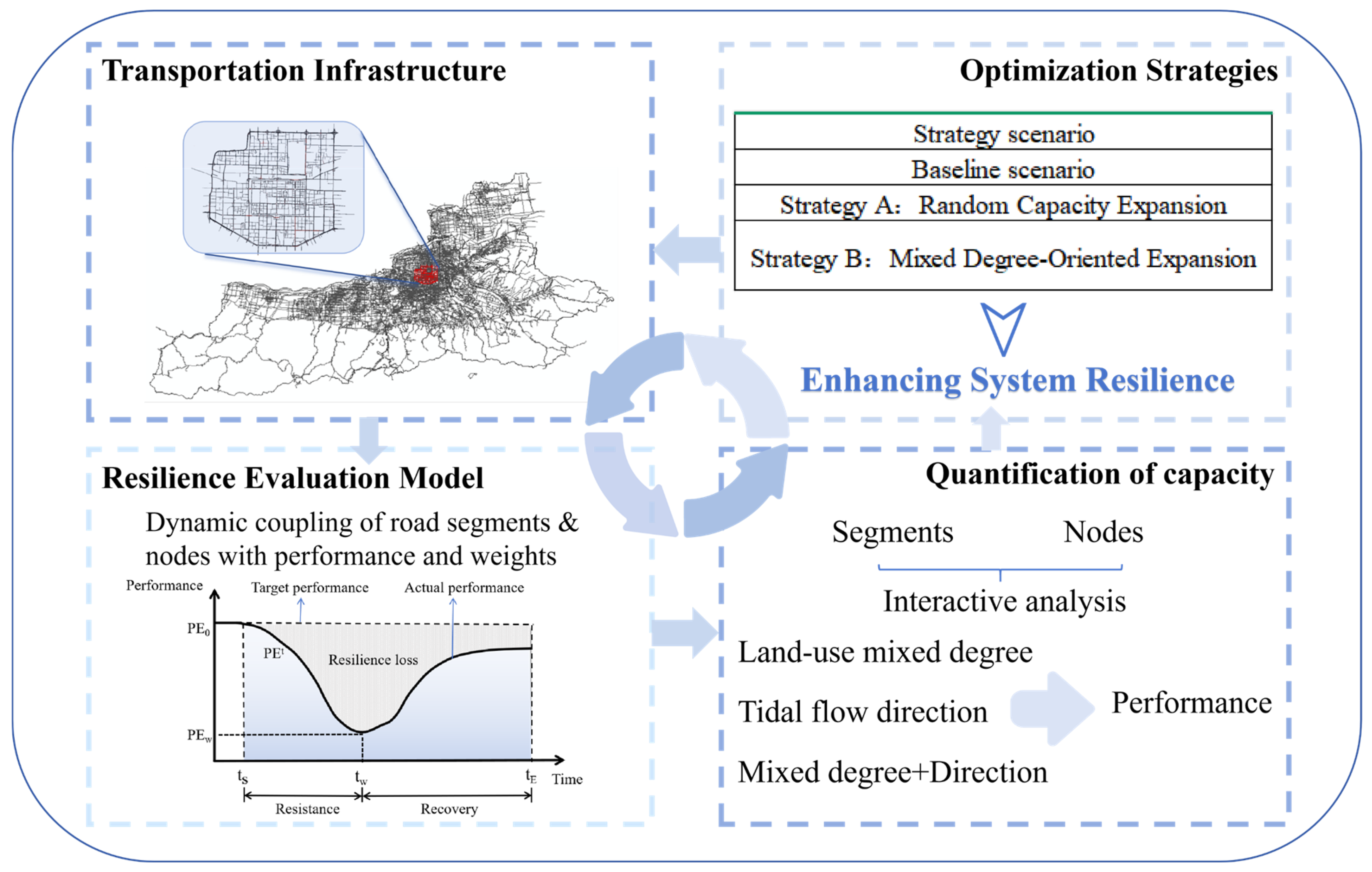
Based on the clarified concept of transportation network resilience, this study is organized into three parts. First, a road-network resilience assessment model is developed. Second, effects of land-use mix levels and tidal traffic-flow direction on performance variation of road segments and nodes are investigated. Third, a resilience enhancement strategy is proposed based on these findings and a simulation is conducted to validate effectiveness of the proposed strategy. Figure 2 provides an overview.
Figure 2.
Framework for assessing and optimizing urban road network resilience.
2.2. Road Network Construction
Based on graph theory, an urban road system is abstracted as a directed weighted graph . Here, the node set represents road intersections, with being the total number of nodes. Edge set represents road segments connecting two intersections. Within the directed graph, a directed edge represents the directed road segment from node to , whose reverse segment is denoted as , where and are treated as two independent edges.
2.3. Road Network Resilience Assessment Model
2.3.1. Road Segment Performance Assessment Indicators
Road segment importance is closely related to urban spatial function distribution. Areas with a high land-use mix intensity tend to generate multi-directional overlapping traffic demands due to their functional complexity, making segments in these areas priority targets for road network management during morning peak hours. This paper introduces the land-use mix entropy model [44]. A 500 m buffer is established on both sides of each segment midline in the road network as a basic research unit to quantify land-use mix intensity within segment buffer area [45], as shown in Equation (2).
where represents the land-use mix entropy of the road segment , with a higher value indicating greater land-use mix functionality, denotes the total number of land use categories, is the proportion of area occupied by land-use type within the 500 m buffer of road segment , satisfying . Because land-use information is derived from POI data, parcel boundaries and precise area shares are unavailable. Therefore, is treated as a functional weight. Equal weights are assigned to categories that appear within a buffer: if categories appear, , categories not appearing take . When , the limit convention is applied. Higher entropy indicates higher land-use mix within 500 m of a segment. High mix implies that morning peak demand may be generated and attracted simultaneously for multiple purposes and time patterns, such as commuting, school trips, medical visits, and shopping. This can induce spatiotemporal superposition of multi-source and multi-directional flows in local networks. It should be noted that the buffer zones generated by this method may overlap between adjacent and parallel road segments, meaning that the mixed-use functionality of some areas may be counted multiple times across different segments. Such spatial overlap objectively reflects the interaction between urban transportation and land use, indicating that a single land parcel may simultaneously influence the transportation demand of multiple adjacent roads.
The importance of a road segment is also influenced by its design classification [46,47]. In China, urban roads are categorized into four grades based on traffic volume, service function, and design parameters: expressway, arterial road, collector road, and local road. This study assigns them values of 4, 3, 2, and 1, respectively [48]. The formula for calculating the road grade weight is defined as Equation (3):
where is the grade weight of road segment , is the assigned grade value of road segment .
Considering the above influencing factors, the comprehensive importance index of the road segment is shown in Equation (4), where weight coefficients and are the coefficients for the land-use mix intensity weight and the grade weight, respectively, satisfying . In this study, the road network’s grade and mix intensity are considered equally important; therefore, both and are assigned a value of 0.5 [49,50,51,52].
Quantitative analysis of road segment performance serves as a critical link connecting land-use mix intensity and traffic operational conditions. Existing research commonly uses travel time as a measure of road segment performance, for instance, utilizing time delay data to directly reflect actual congestion levels [53]. This study adopts the dynamic travel time ratio as the measurement indicator, defined as the ratio of free-flow travel time on a road segment to the actual vehicle travel time under real traffic conditions, as shown in Equation (5):
where is the performance value of the road segment during time window . A value closer to 1 indicates an operational state nearer to free-flow conditions and better performance. This indicator directly quantifies the real-time functional state of a road segment under disturbance. and are the free-flow travel time and actual average travel time of the road segment during time window , respectively. is computed as , where is segment length and is the design speed. Design speed was specified as follows [54]: expressway 60–100 km/h, arterial 40–60 km/h, collector 30–50 km/h, local 20–40 km/h. Midpoint values are used in implementation: 80, 50, 40, and 30 km/h for expressway, arterial, collector, and local roads, respectively. Actual travel time is derived from Baidu Maps API (Baidu Maps Open Platform Traffic API, accessed in October 2024, queried via Python 3.9 (64-bit)), which provides 5 min segment average speed, capturing real-time traffic state.
The performance of all road segments in the network is calculated by taking the weighted sum of each segment’s comprehensive importance weight and its performance value, as shown in Equation (6).
where is the overall performance of all road segments in the network during time window .
2.3.2. Node Performance Assessment Indicators
Nodes located in areas of high land-use mix intensity zones experience multi-directional and multi-purpose traffic flows during morning peak hours, due to the diversity of surrounding land functions. This study also employs a land-use mix entropy model, as shown in Equation (7), to establish a circular zone with a radius of 500 m centered on the node’s geometric center as the fundamental research unit. This approach quantifies the land-use mix intensity within a 500 m radius surrounding the node.
where is the land-use mix entropy value of node , denotes the proportion of area occupied by land-use type within the 500 m buffer zone of node , satisfying .
In complex network theory, closeness centrality is calculated by taking the reciprocal of the sum of the shortest physical path distances from a given node to all other nodes in the network, evaluating its overall proximity to the rest [49]. This study adopts closeness centrality as an indicator to measure a node’s global positional criticality, as shown in Equation (8). This indicator quantifies effective accessibility of a node under real-time traffic conditions.
where is the closeness centrality of node , is the shortest physical distance (km) from node to any other node , measured in kilometers. It refers to shortest-path distance on road network graph. It is obtained by shortest-path computation on directed weighted road graph, where edge weight equals actual segment length.
Synthesizing the above influencing factors, the comprehensive importance index of nodes is shown in Equation (9).
where represents the comprehensive importance of the node . and are the coefficients for the land-use mix intensity weight and structural weight of the node, respectively, satisfying . This paper considers the functional and structural aspects of nodes equally important. Therefore, both and are set to 0.5.
Based on the definition of node closeness centrality, this paper introduces a dynamic temporal closeness centrality metric to reflect spatiotemporal costs arising from congestion in real traffic scenarios [48], as shown in Equation (10). This metric characterizes a node’s actual operational performance under real-time traffic conditions by taking the reciprocal of the sum of the shortest travel times from that node to all other nodes in the network.
where is the performance metric of the node within the time window , is the shortest travel time from the node to any other node within the time window .
The performance of all nodes in the road network is calculated by the weighted summation of each node’s weight and its performance value, as shown in Equation (11).
where is the overall performance of all nodes in the road network within time window .
2.3.3. Road Network Performance Assessment Indicators
The overall performance of a road network is the integrated outcome of the coordinated interaction between road segments and nodes under spatial connectivity and functional dependence. The two components form a mutually supportive relationship, such that degradation on either side can destabilize the whole system. Accordingly, this study adopts the product of the performance of all road segments and nodes across the network as a quantitative indicator of the network’s operational state, as shown in Equation (12). Representing the overall network performance through additive aggregation of segments and nodes introduces a masking effect where strengths compensate for weaknesses. That is, the outstanding performance of one component may to some extent conceal severe deficiencies in others, thereby maintaining the overall metric at a relatively high level without accurately reflecting the structural risks present in the system. In contrast, the product operation is more sensitive to localized performance variations within the system. When any dimension (road segment or node) exhibits performance shortcomings, the overall metric will simultaneously show a significant decline, thereby more accurately revealing the system’s bottleneck constraints and vulnerabilities.
where is the overall performance value of the road network within the time window .
Based on the resilience triangle theory proposed by M. Bruneau [43,55,56], this paper quantifies the road network resilience value by calculating the ratio of the area between the actual performance curve and the ideal performance curve, as shown in Equation (13).
where is the resilience value of the road network during the morning peak period, with a value range of [0, 1], is the start time of the morning peak, is the end time of the morning peak, is the baseline performance value of the road network under steady state before the morning peak begins.
3. Result
3.1. Study Area and Data Foundation
The study focuses on the road network within the Second Ring Road of Xi’an, China, which constitutes the city’s most traffic-intensive core area. It features a highly complex network structure and a dense mixture of residential and commercial land uses. The area exhibits high spatial heterogeneity in land-use patterns. During the morning peak hours, diverse travel demands, including commuting, business, medical, and educational trips, intensely overlap in both space and time, leading to pronounced traffic pressure. From a spatial perspective, the area within the Second Ring Road shows clear land-use functional heterogeneity. Areas with high land-use mix intensity are mainly concentrated in the central business district, major transport hubs, and clusters of public service facilities. Such areas typically integrate residential, commercial, educational, and medical functions, showing stronger functional interweaving and higher trip generation and attraction intensity.
The datasets employed in this study comprise the following components: Road network topology data extracted from OpenStreetMap (official web platform, accessed in October 2024), encompassing 370 bidirectional road segments and 69 intersection nodes. Traffic congestion data obtained from the Baidu Maps API, covering a 5-day weekday period in October 2024 during the morning peak hours (07:00–10:00), with data recorded at 5 min intervals. Land-use data derived from Baidu Maps Points of Interest (POI) (Baidu Maps Open Platform Place API, accessed in October 2024, queried via Python 3.9 (64-bit)), based on which the study area is categorized into five primary functional zones: residential, commercial, educational, medical, and municipal facilities. This classification comprehensively considers the traffic generation and attraction effects of different functional areas during the morning peak period. Residential areas primarily serve as the origins of commuting trips. Schools and hospitals generate concentrated directional flows associated with class start times and medical appointments. Municipal facilities are characterized by regular official commuting patterns. In contrast, recreational land uses such as parks and scenic spots exert minimal influence on peak-hour traffic and are therefore excluded from the primary functional classification system. It should be noted that in resilience analysis, buffer delineation around segments and nodes lacks universally fixed physical boundaries. Existing studies often define such spatial ranges based on walking accessibility, typically corresponding to a spatial scale of about 480–720 m [57]. Regarding selection of buffer size, 500 m, 800 m, and 1000 m are commonly adopted in practice [58]. In transportation and land-use interaction research, North American studies commonly adopt 400–800 m, while European studies often use about 700 m [59]. Under Asian urban contexts, some scholars, based on a Seoul metro passenger survey, identify about 460 m as an influential radius [45]. From a planning–practice perspective, 500 m is widely regarded as a basic community life circle or walking service radius. Relevant planning standards commonly adopt 500 m as a reference service range for community-level facilities such as primary schools [60]. Considering that land-use mix intensity in this study covers multiple functions such as residence, commerce, education, and healthcare, and that these functions can directly affect road traffic, a 500 m buffer is adopted for both segments and nodes in the resilience assessment framework. This study employs 10 min time windows, spanning from 7:00–7:10 to 9:50–10:00, dividing the analysis period into 18 consecutive time windows.
3.2. Road Segment Performance Analysis
This section uses statistical analysis and visualization to systematically present associations between land-use mix intensity and road segment performance. The analysis first examines the overall relationship between mix intensity and performance, then introduces direction to explore the spatial superposition effect between mix intensity and tidal commuting flow.
3.2.1. Land-Use Mix Intensity-Segment Performance Analysis
To systematically analyze the impact of land-use mix intensity on road segment performance, this study first quantifies the mix intensity of each road segment based on an entropy model. During computation, equal weights are assigned to land-use types that appear within each segment buffer, given limited availability of parcel boundaries and area shares. Based on this approach, the land-use mix intensity values of 370 bidirectional road segments are derived. The calculation results show that the entropy values of all road segments can be summarized into four distinct numerical levels. Accordingly, these values are categorized into four levels: Level 1: single land-use mix intensity, Level 2: low land-use mix intensity, Level 3: medium land-use mix intensity, and Level 4: high land-use mix intensity (representing areas with overlapping functions such as commercial, residential, educational, and medical facilities). To characterize the temporal performance variations of road segments with different mixing levels during the morning peak, the average performance value of all road segments within each mixing level is calculated for every 10 min time window. This serves as a representation of the overall performance of segments at that mixing level for a given time interval. Subsequently, the range of variation and median value of the average performance of road segments across the 18 morning peak time windows are statistically summarized for each mixing level. The median value reflects the typical performance level of road segments at a given mixing level across most periods of the morning peak, while the variation range measures the stability of these segments under the influence of fluctuating morning peak traffic flows. Table 1 presents the median values and variation ranges of the average performance for the four types of mixing level road segments across 18 consecutive time windows during the morning peak.
Table 1.
Statistical summary of average performance values for segments under different mix intensity levels.
As shown in Table 1, as the mixing level increases, the median value of road segment performance decreases significantly while the range of variation widens. Segments with a high land-use mix intensity (Level 4) exhibit a median performance value of 0.46, which is considerably lower than that of single-function segments (Level 1) with a median value of 0.87, indicating that highly mixed segments experience more severe performance degradation during the morning peak period. Meanwhile, segments with moderate to high mixing levels (Levels 3 and 4) display a considerably wider range of performance variation, suggesting greater sensitivity to fluctuations in traffic flow and reduced operational stability.
To further test statistical significance of performance differences across mix intensity levels, a nonparametric Kruskal–Wallis H test is applied to segment performance data for four levels. Results indicate highly significant differences among levels (H = 215.36, p = 0.13 × 10⁻³), supporting that land-use mix intensity acts as a key determinant of segment performance with strong statistical reliability. To quantify practical significance, effect sizes are evaluated using Cliff’s Delta. Following guidance [61], |δ| ≥ 0.43 indicates a large effect, 0.28 ≤ |δ| < 0.43 indicates a medium effect, and smaller values imply limited practical difference. The corresponding effect sizes are reported in Table 2.
Table 2.
Effect sizes of average performance values for segments under different mix intensity levels.
Effect-size results show that high mix intensity segments (Level 4) differ from Levels 1–3 with medium-to-large effects (δ ≥ 0.327), with the largest contrast observed against single-function segments (Level 1, δ = 0.722). Medium mix intensity segments (Level 3) differ from low mix intensity segments (Levels 1–2) with medium effects. Differences between Levels 1 and 2 remain relatively small. Overall, both statistical tests and effect-size analysis reveal a clear gradient: segment performance declines systematically with increasing mix intensity level.
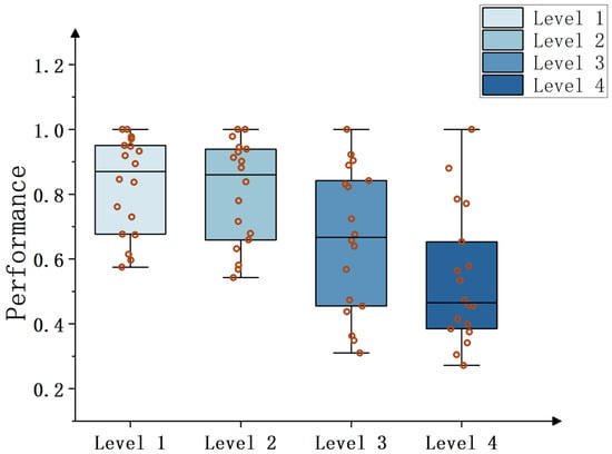
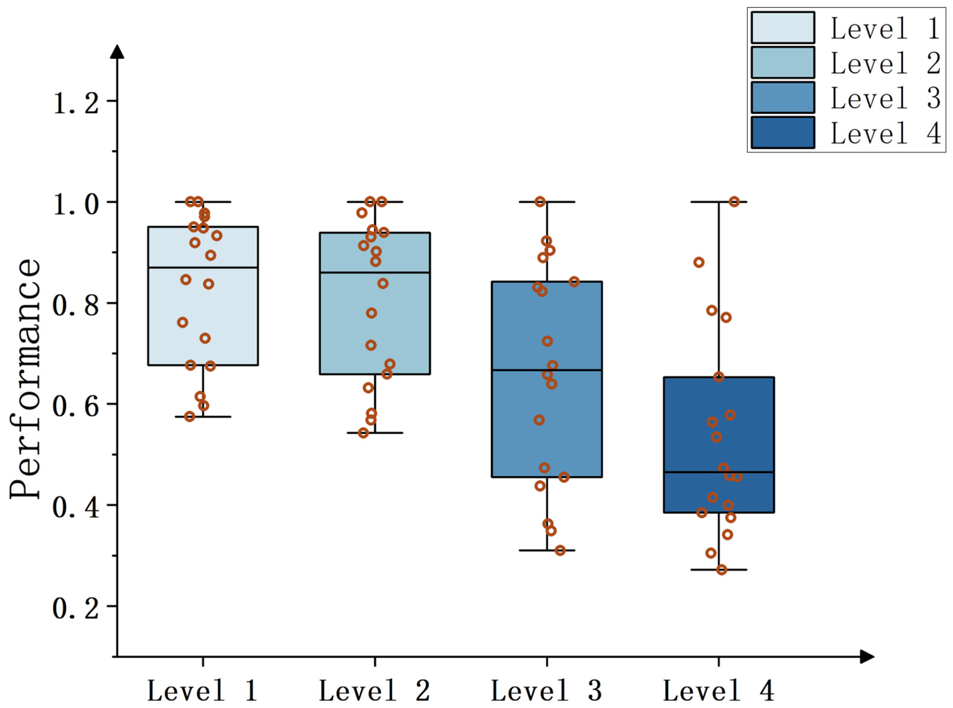
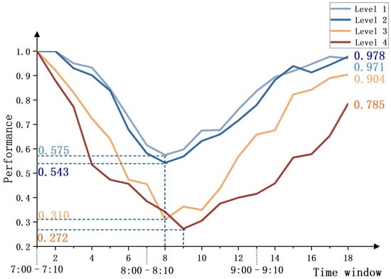
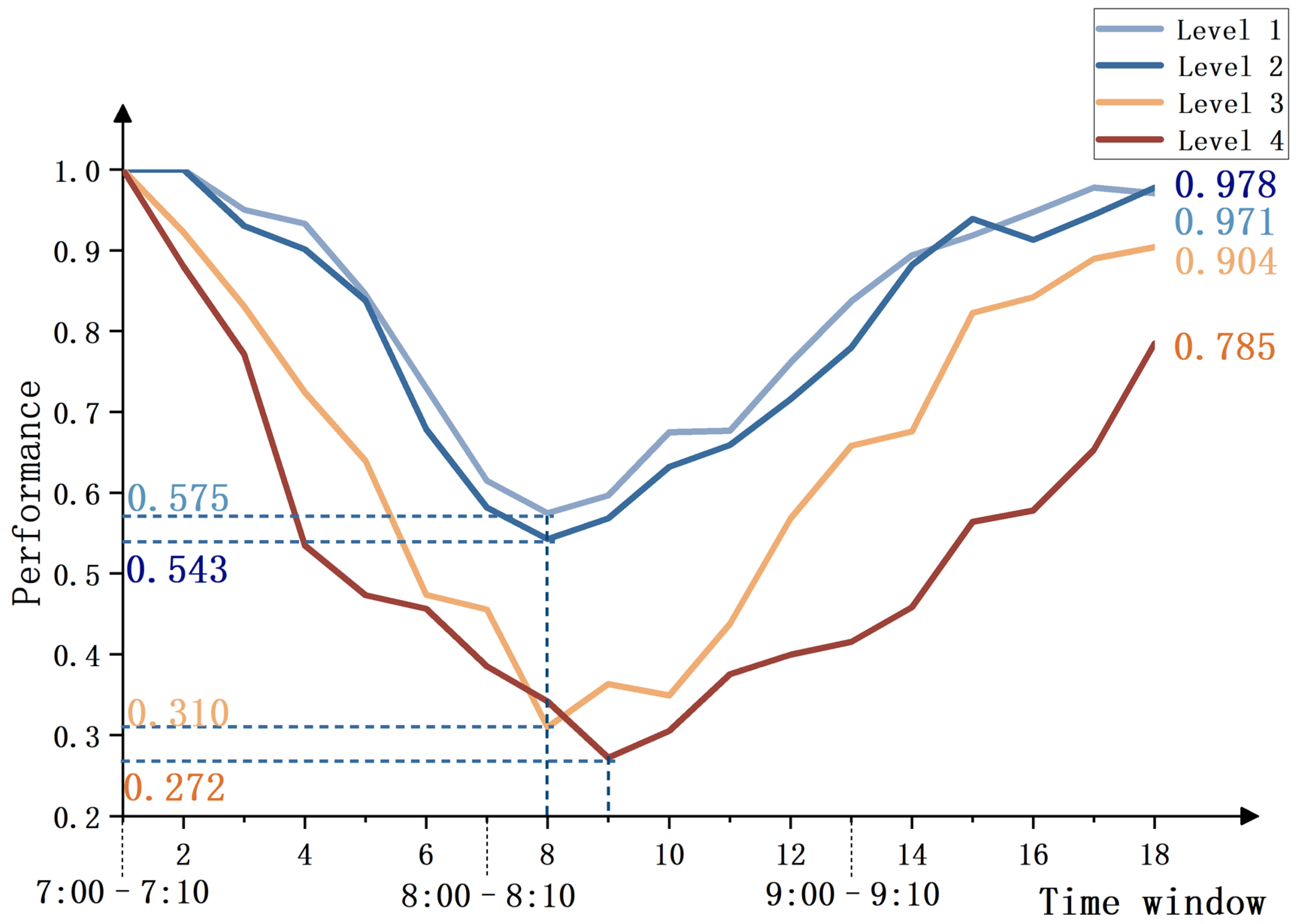
Figure 3 and Figure 4 present the boxplots and line charts of the average performance values of road segments with different land-use mix levels across the 18 times windows. These visualizations further illustrate the relationship between land-use mix intensity and road segment performance during the morning peak period from both statistical distribution and dynamic temporal evolution perspectives.
Figure 3.
Boxplots of average performance values distribution for segments with different mix intensity levels across 18 times windows.
Figure 4.
Dynamic evolution curves of average performance values for segments with different mix intensity degrees across 18 times windows.
From the boxplot in Figure 3, it can be observed that as the level of land-use mix increases, the boxes progressively shift downward and exhibit a wider distribution range. Specifically, the average performance values of single land-use mix intensity segments (Level 1) are concentrated in higher value range with compact box shapes, indicating relatively stable operational conditions and minimal external interference. In contrast, high land-use mix intensity segments (Level 4) display a pronounced downward shift of the box, with most performance values clustered at lower levels, reflecting intense performance fluctuations and poor stability in this mixing level of road segments.
As illustrated in Figure 4, compared with single and low land-use mix intensity segments (Levels 1 and 2), the medium and high land-use mix intensity segments (Levels 3 and 4) exhibit significantly steeper declines in their average performance curves, lower trough values, and noticeably delayed recovery process, a typical low-resilience pattern. In particular, the land-use mix intensity segments (Level 4) nearly remain at the lowest performance level throughout the entire morning peak period: their performance drops to a minimum of 0.272 at time window 9 and recovers only to 0.785 by the end of the peak period. This pattern indicates a distinct feature of rapid degradation and slow recovery, reflecting limited traffic resilience. By contrast, the single land-use mix intensity segments (Level 1) demonstrate a much higher minimum performance value of 0.575, approximately 2.1 times greater than that of the high land-use mix intensity segments. Furthermore, their performance gradually recovers to near the initial level by the end of the morning peak.
Figure 3 and Figure 4 indicate that an increase in land-use mix intensity during the morning peak period not only systematically reduces the overall performance level of road segments and amplifies their volatility, but also exacerbates the severity of performance degradation and delays the recovery process under traffic disturbances.
3.2.2. Direction-Mix Intensity-Segment Performance Analysis
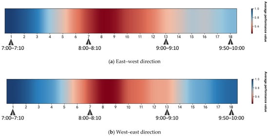
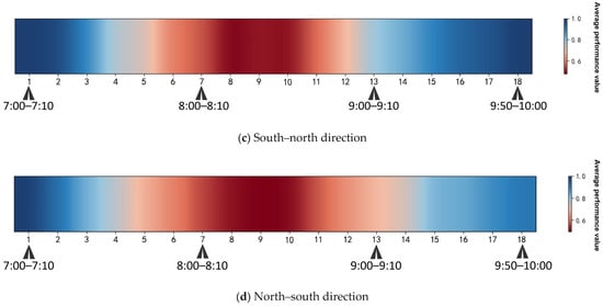
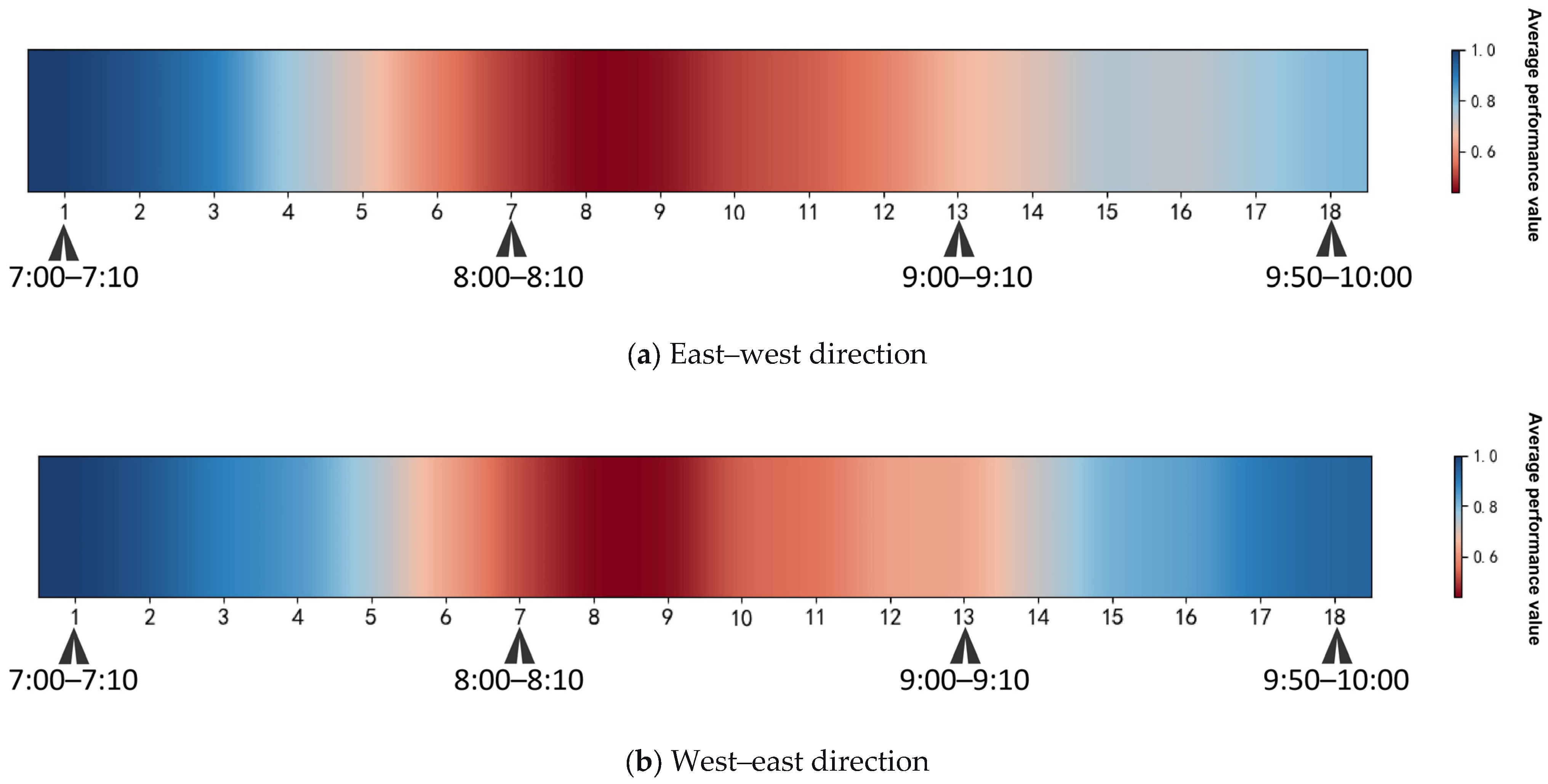
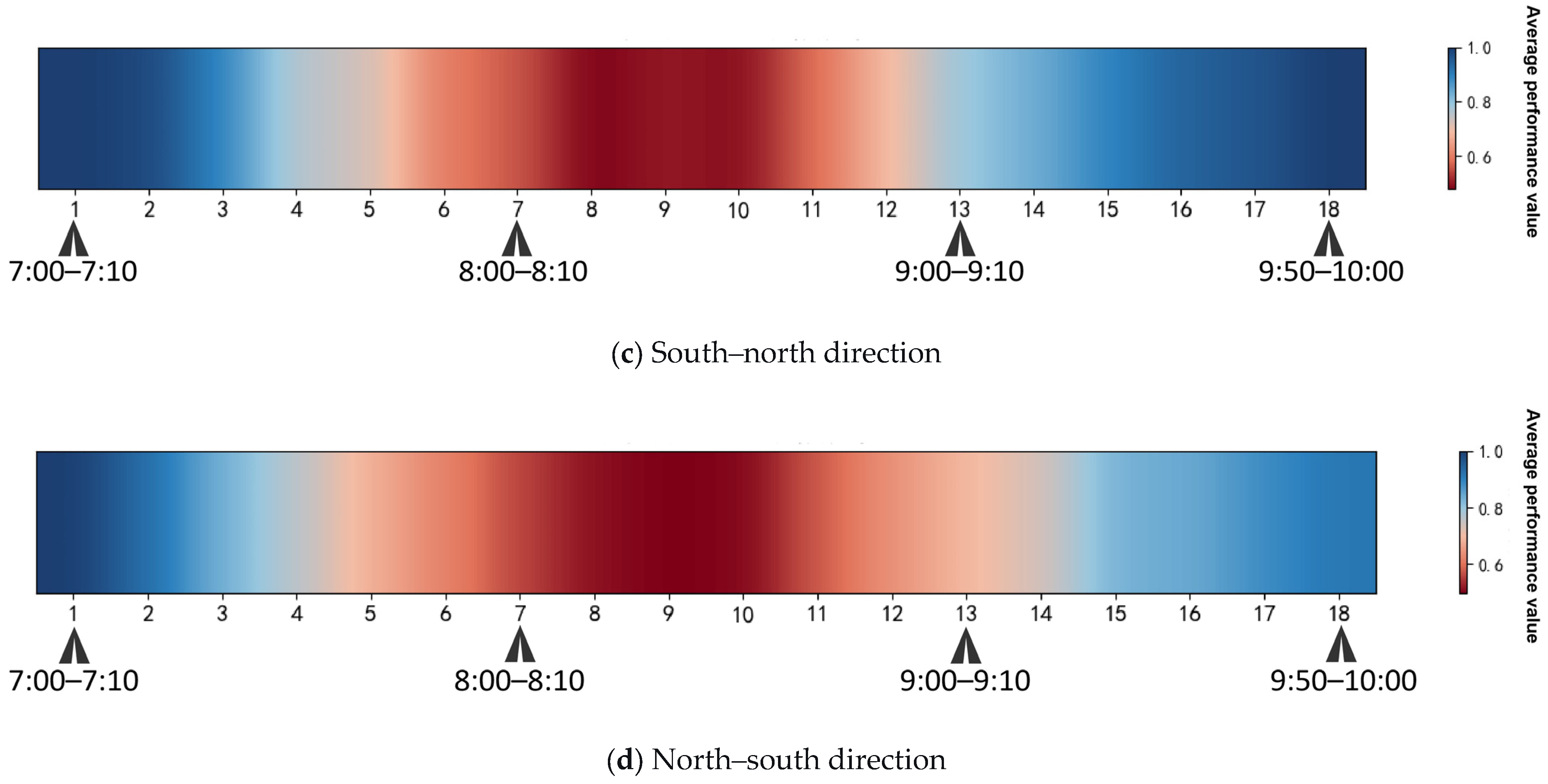
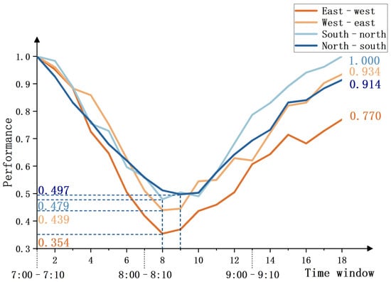
Following the previous analysis of mix intensity, this section further incorporates the directional dimension to examine the combined effects between tidal traffic flow and land-use mix intensity during the morning peak period. Firstly, based on the average performance heatmaps and dynamic variation line charts of road segments in different directions as shown in Figure 5 and Figure 6, respectively, this study compares the performance of segments in opposite directions within the same corridor. For east–west corridors, the analysis contrasts the performance between eastbound and westbound segments, while for north–south corridors, it compares northbound and southbound segments. Through this comparison, the study identifies the dominant flow directions within each corridor that bear the main traffic pressure during the morning peak hours.
Figure 5.
Heatmaps of average performance values for segments in different directions across 18 times windows.
Figure 6.
Dynamic evolution curves of average performance values for segments in different directions across 18 times windows.
In Figure 5, deeper red hues indicate lower performance, while deeper blue hues represent higher performance. Performance values range from 0 to 0.5 representing the low-performance range. Analysis reveals that the east–west and north–south road segments enter the low-performance state earlier than their opposite directions, with the red areas persisting for a longer duration. Moreover, during the late recovery phase between time windows 15 and 18, the performance recovery level of these segments is noticeably delayed, particularly for the east–west direction, which shows a lower degree of performance restoration.
Figure 6 further confirms this trend from a dynamic process perspective: the performance curves of the east–west and north–south segments remain almost consistently below those of their opposite direction counterparts throughout the entire morning peak period. By the end of the morning peak, the performance values of these two directional segments only recovered to 0.770 and 0.914, respectively, both lower than their opposite directions. Integrating the findings from Figure 5 and Figure 6, it can be concluded that the east–west and north–south directions are the primary pressure directions during the morning peak, exhibiting greater vulnerability, with congestion issues characterized by both persistence and delayed recovery.
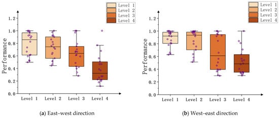
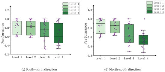
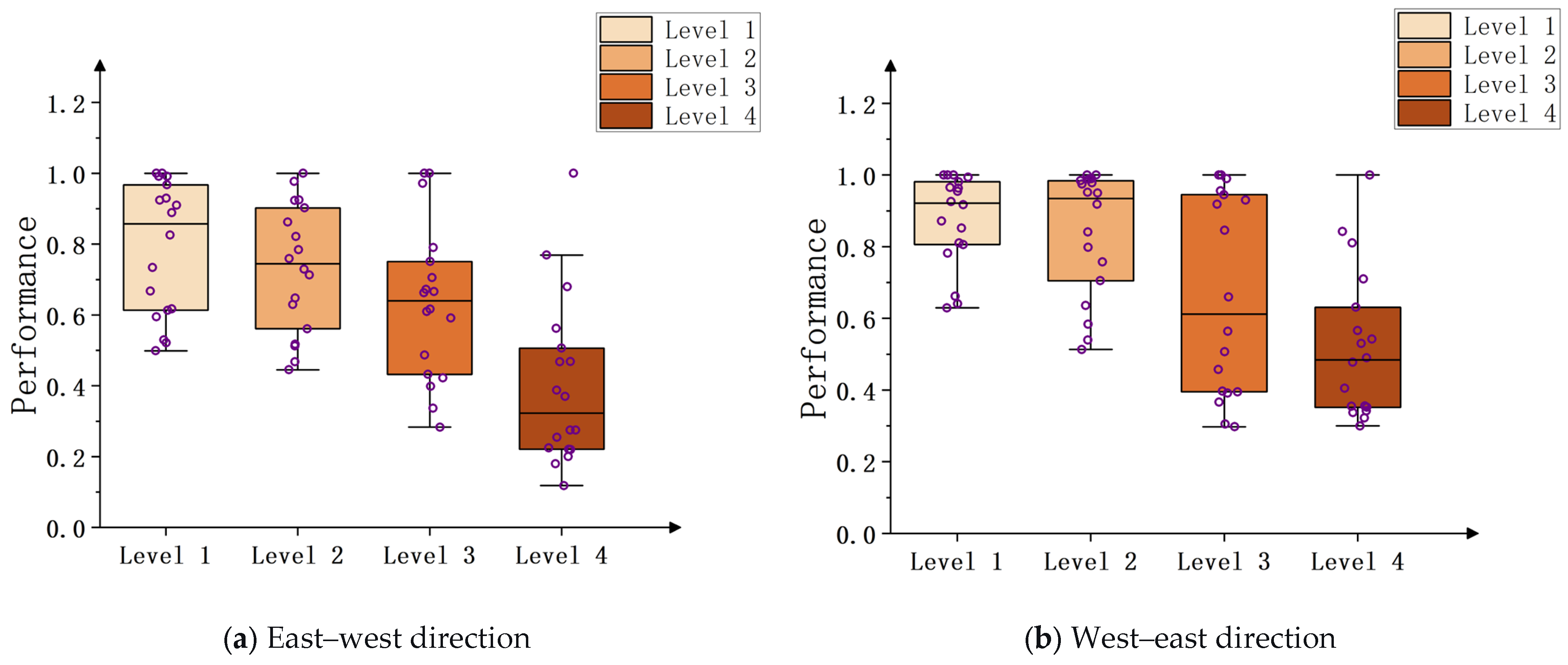
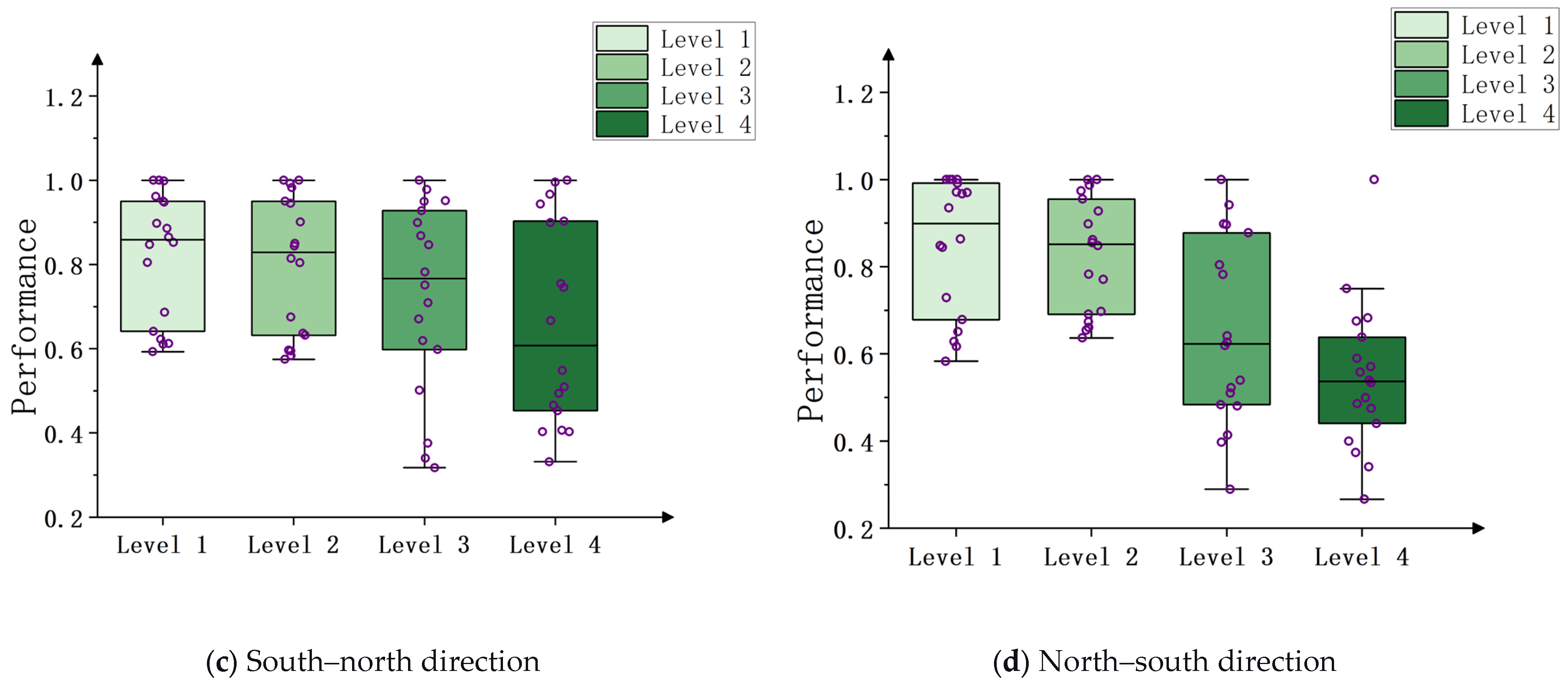
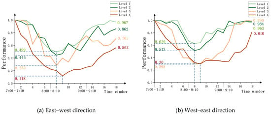
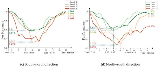
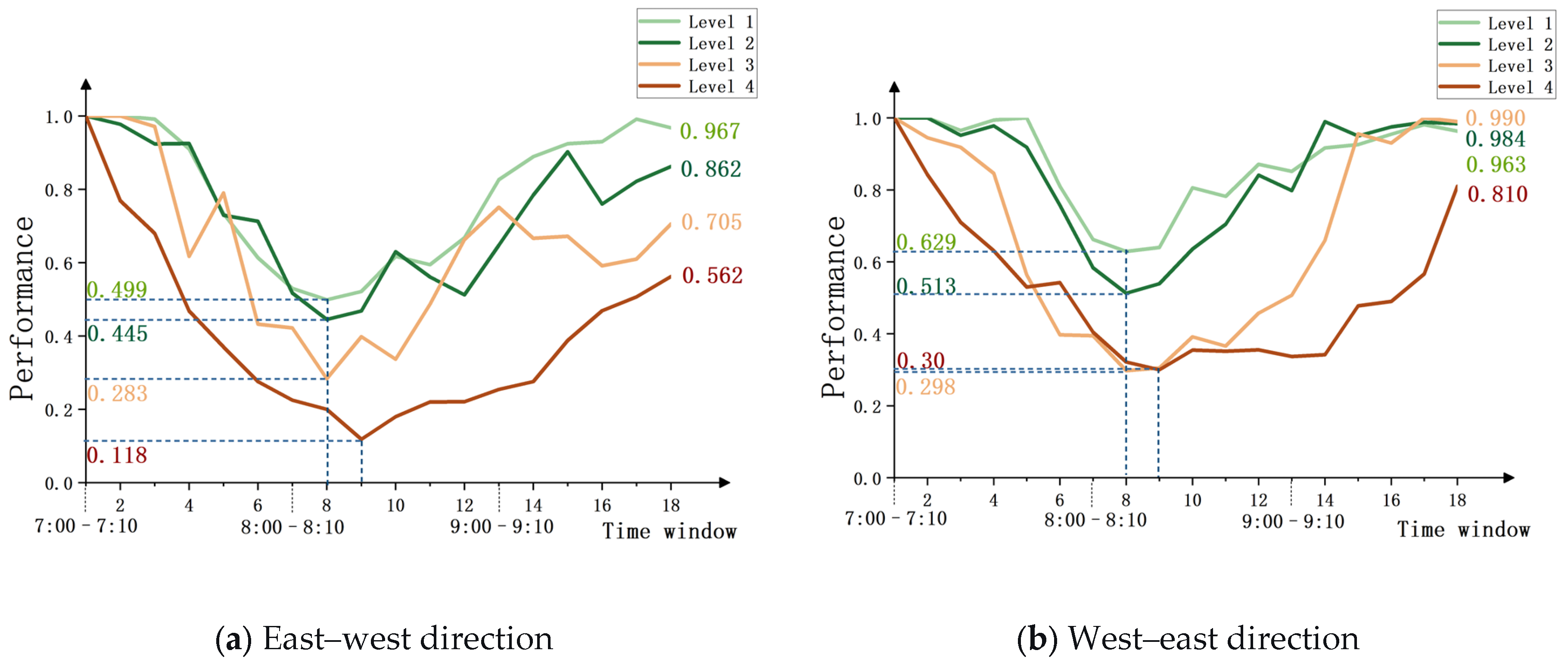
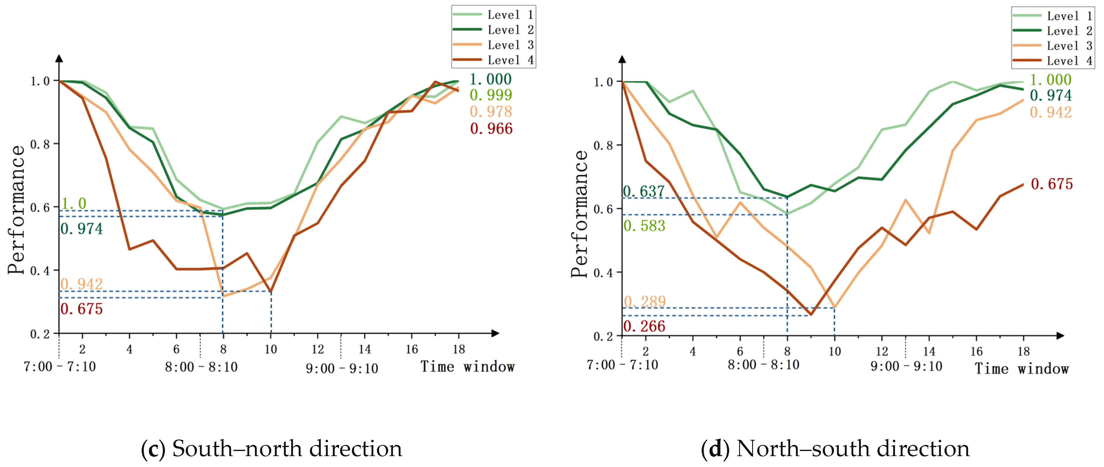
Secondly, this study extends the analysis by presenting boxplots of average performance distribution and dynamic line charts for road segments with varying mixing levels under different traffic directions, as shown in Figure 7 and Figure 8, respectively. These visualizations facilitate the analysis of the interaction between the land-use mix intensity and the traffic direction.
Figure 7.
Boxplots of average performance values distribution for segments with different mix intensity levels under various traffic directions.
Figure 8.
Dynamic evolution curves of average performance values for segments with different mix intensity levels under various traffic directions.
The statistical distribution in Figure 7 reveals that dominant traffic pressure exacerbates the performance vulnerability of high mix intensity (Level 4) segments. In the east–west corridor, the median performance value for high mix intensity segments in the east–west dominant direction (Figure 7a) is exceptionally low, with a concentrated distribution of low-performance values. In contrast, the same-level segments in the opposite west–east direction (Figure 7b) exhibit a clear improvement in performance distribution. A similar pattern is also found in the north–south corridor, revealing a superimposed effect between high land-use mix intensity and mainstream traffic direction pressure.
Figure 8 validates the mentioned effect from a dynamic evolution perspective. Along the dominant pressure directions: east–west and north–south, high mix intensity segments (Level 4) exhibit greater performance degradation and lower trough values compared to their opposite-direction counterparts. During the recovery phase, performance rebounds more slowly, with performance levels remaining substantially lower than the initial state by the end of the morning peak. Specifically, in the east–west corridor, high mixing segments (Level 4) in the east–west direction deteriorated to a trough value of 0.118 during time window 9, recovering only to 0.562 by the end of the morning peak. In contrast, the comparable west–east segments of the same level reach a trough of 0.30 and recover to 0.810 by the end, demonstrating a faster and more complete recovery. A similar pattern is observed for the dominant pressure direction in the north–south corridor. Integrating the evidence from Figure 7 and Figure 8, it can be concluded that the spatial coincidence of high mix intensity areas with primary commuter directions creates a compounding effect of mixed-traffic intensity and tidal flows, which exacerbates performance degradation and delays recovery across these segments.
3.3. Node Performance Analysis
3.3.1. Land-Use Mix Intensity-Node Performance Analysis
Similarly to the road segment analysis, this study first calculates the land-use mix intensity values of 69 nodes based on the entropy model and classifies them into four levels according to their numerical value distribution. Table 3 presents the median values and fluctuation ranges of the average performance of nodes with different land-use mix intensity levels during the morning peak period.
Table 3.
Statistical summary of average performance values for nodes under different mix intensity levels.
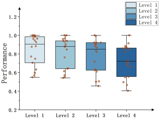
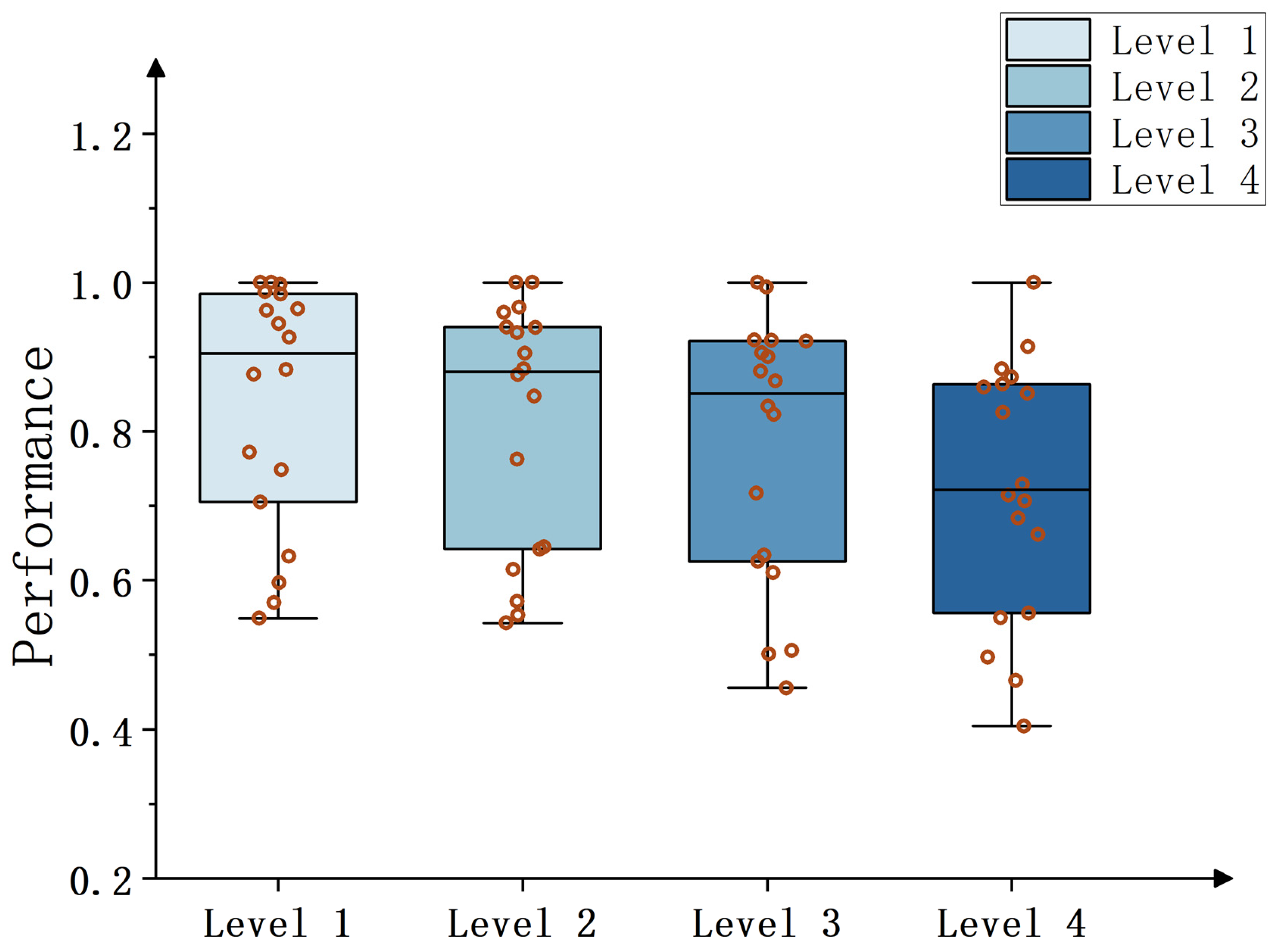
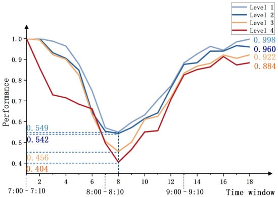
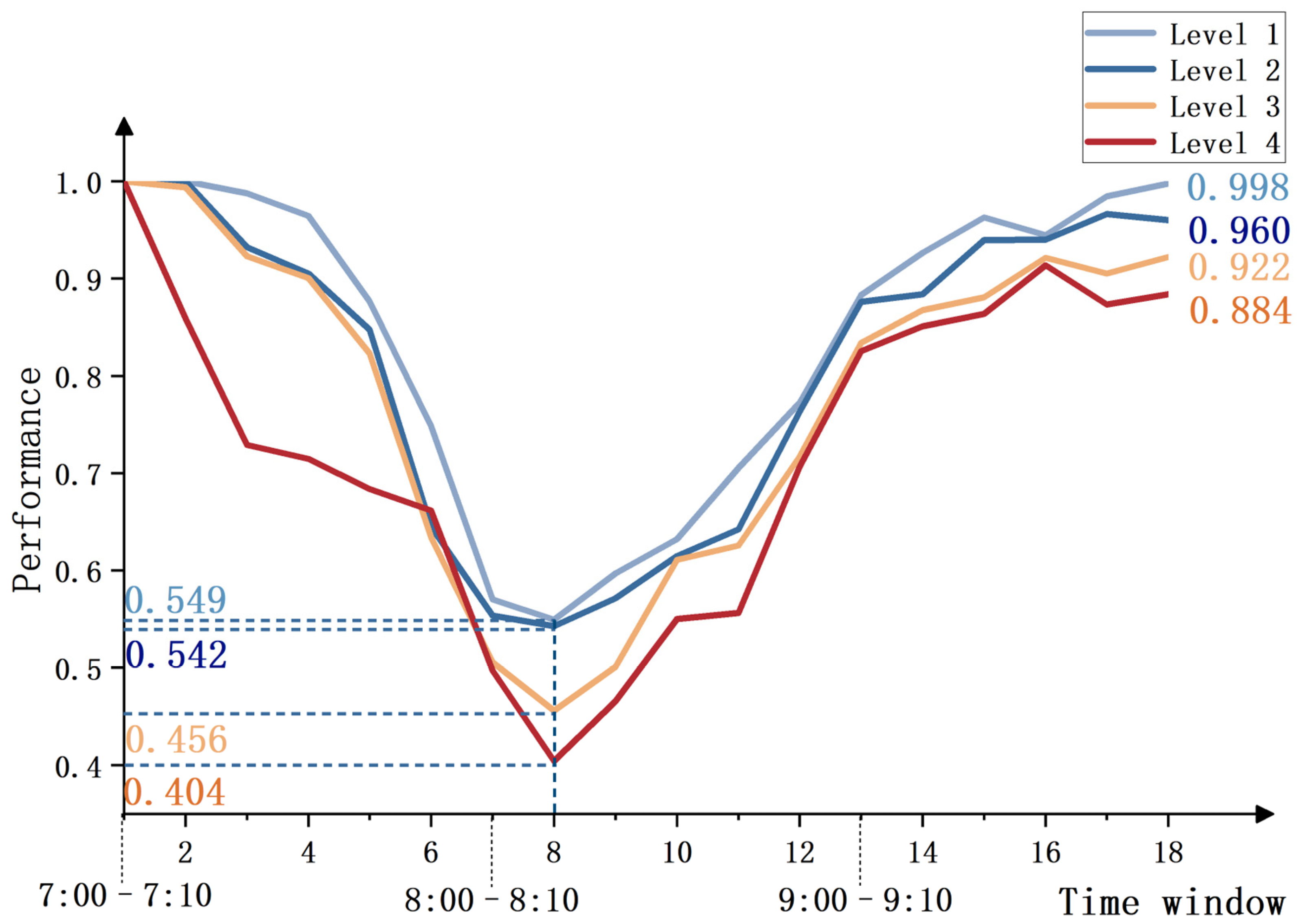
According to the analysis results in Table 3, node performance exhibits a systematic declining trend with the increase in land-use mix intensity. Specifically, the median performance value of high mix intensity nodes (Level 4) is only 0.72, which is significantly lower than that of single mix intensity nodes (Level 1) with a median value of 0.91. Meanwhile, their performance exhibits a wider fluctuation range and greater instability in performance states. Figure 9 and Figure 10 present the boxplots and line charts of the average performance values of road nodes with different land-use mix intensity levels across the 18 times windows.
Figure 9.
Boxplots of average performance values distribution for nodes with different mix intensity levels across 18 times windows.
Figure 10.
Dynamic evolution curves of average performance values for nodes with different mix intensity levels across 18 times windows.
A Kruskal–Wallis H test is conducted to examine performance differences among node mix intensity levels. Results show no statistically significant difference among the four levels (H = 5.78, p = 0.123). Although statistical significance is not reached, Cliff’s Delta is further used to quantify practical differences among levels. The corresponding effect sizes are reported in Table 4.
Table 4.
Effect sizes of average performance values for nodes under different mix intensity levels.
Cliff’s Delta results indicate noticeable differences between selected levels. In particular, performance contrast between Level 1 and Level 4 reaches a medium effect size (Cliff’s Delta = 0.407), suggesting weaker node performance in high mix intensity areas. The effect size between Levels 2 and 3 is small (Cliff’s Delta = 0.160), implying limited difference, while the contrast between Levels 3 and 4 shows a small effect (Cliff’s Delta = 0.222), further supporting performance attenuation in high mix intensity areas.
Figure 9 presents the performance distribution characteristics of nodes with varying mix intensities through box plots. It can be observed that the boxes for single and low mix intensity nodes (Levels 1 and 2) are compact, indicating minimal overall performance fluctuations. In contrast, the boxes for medium and high mix intensity nodes (Levels 3 and 4) exhibit a noticeable downward shift and expanded range, with a dense distribution of lower values. This visually demonstrates their lower performance levels and poorer operational reliability.
Figure 10 reveals the performance evolution characteristics of nodes with different mix intensities during the morning peak period from a dynamic perspective. High mix intensity nodes (Level 4) experience the most severe performance degradation under disturbance, with a trough value dropping as low as 0.404. During the recovery phase, their performance rebound rate also delays significantly. By the end of the morning peak, single mix intensity nodes (Level 1) largely return to their initial performance state, while high mix intensity nodes only recover to 0.884. In summary, due to sustained multi-purpose travel demand, high land-use mix intensity nodes face greater traffic pressure during the morning peak, exhibiting deficiencies in both resistance and recovery capabilities.
3.3.2. Correlation and Differences Between Node and Segment Performance
Comparing segment and node performance in Table 1 and Table 3 shows that at the high mix intensity (Level 4), the median performance value of nodes is 0.72, approximately 1.6 times that of segments. By comparing Figure 4 and Figure 10, it can be observed that the performance trough of high mix intensity nodes is 0.404, exceeding the 0.272 trough value for high-mix road segments. Moreover, by the end of the morning peak, the recovery level of high mix intensity nodes is significantly better than that of segments. These differences may stem from their distinct functional roles and physical characteristics within the road network. As traffic hubs, junctions are typically equipped with signal control systems, allowing for more flexible management of accumulated traffic flow and demonstrating stronger self-organizing capability. In contrast, segments serve as linear channels where congestion tends to form rapidly and becomes difficult to dissipate internally once traffic demand exceeds their physical capacity, resulting in more severe performance degradation.
Results above indicate that, under morning peak congestion as a representative demand-driven recurrent disturbance scenario, segments and nodes located in high land-use mix areas generally exhibit more severe performance deterioration and more pronounced recovery delay. Compared with low-mix or single-function areas, high-mix areas show lower performance troughs, larger performance variability, and less complete recovery by the end of morning peak, indicating relatively higher vulnerability during morning peak periods. Land-use types in the study area are classified into five categories: residential, commercial, school, hospital, and municipal facilities. A buffer containing at least four categories is defined as high land-use mix. This pattern suggests that, in dense urban cores, high land-use mix does not necessarily represent balanced and random co-location of multiple functions. Instead, it often reflects a composite spatial form centered on high trip-generating public service facilities, such as schools and hospitals, with residential, commercial, and municipal-service functions superimposed.
Under this spatial structure, performance disadvantages observed in high-mix areas during morning peak cannot be attributed to a single mechanism. On one hand, schools and hospitals generate concentrated school-arrival and medical-visit trips, together with associated pick-up and drop-off movements. Such demand is short-duration, high-intensity, and strongly directional, imposing direct operational stress on adjacent segments and nodes. On other hand, strong co-location of multiple functions induces multi-purpose and multi-directional travel behavior. It is also associated with more complex operational interactions, including curbside stopping, frequent lane changes, and intensified turning conflicts. These effects reduce effective capacity on segments and at intersections. Spatial superposition of these mechanisms makes high-mix areas more likely to experience rapid performance decline and slower recovery under morning peak disturbances. Evidence from Figure 4 and Figure 10 further supports this interpretation: for land-use mix Level 4, both segments and nodes show lower trough values, larger fluctuation ranges, and limited recovery near the end of morning peak. This set of observations characterizes operating patterns of road networks under recurrent disturbances for a typical spatial form where high land-use mix is coupled with public service facilities.
Based on segment- and node-level results, reduced resilience of high-mix segments is not solely attributable to higher demand volume. Mixed-use areas often concentrate schools, hospitals, commercial activities, and residential functions. In addition to commuting flows, morning peak periods can involve substantial facility-related short-term behaviors, including pick-up and drop-off, curbside temporary stopping, parking search, and delivery loading and unloading. Such behaviors increase frequency of speed reduction and lane changing, amplify turning conflicts and intersection delays, and thereby reduce effective capacity of segments and intersections. Queue spillback and congestion diffusion become more likely, leading to lower performance troughs and slower recovery. Accordingly, resilience around mixed-use areas depends not only on demand intensity, but also on access organization and convenience, such as curbside pick-up and drop-off management, network capacity, and regulatory policies. It is also closely related to travel-behavior complexity induced by land-use mix. This study identifies that high-mix segments, particularly along predominant tidal commuting directions, exhibit more pronounced performance deterioration and recovery delay. It should be noted that high-mix areas often overlap spatially with high-intensity urban activities, such as employment and commercial concentrations. Therefore, observed performance disadvantages may be partially confounded by activity intensity.
4. Discussion on Mix Intensity-Oriented Spatial Optimization Strategy
High mix intensity areas tend to concentrate multiple urban functions such as residential, commercial, educational, and medical activities. During the morning peak period, segments in these areas simultaneously accommodate commuting trips and various non-commuting travel demands, leading to complex traffic organization and dense conflict points. As a result, their operating performance is more prone to pronounced degradation and delayed recovery. To improve the capacity of critical road segments under resource-constrained conditions, this study proposes a land-use mix–oriented spatial optimization strategy. Specifically, priority is given to enhancing the capacity of key segments located in areas with high land-use mix intensity, so as to strengthen the overall resistance and recovery capability of the road network system. To evaluate the effectiveness of the proposed strategy, one baseline scenario and two spatial optimization scenarios are constructed for comparative analysis. The baseline scenario maintains the original network structure and lane configuration, representing the resilience level of the road network under current conditions during the morning peak disturbance. Strategy A (random capacity expansion) randomly selects 10% of network segments to add one lane, simulating improved traffic efficiency through enhanced management or social resource inputs. Strategy B (mix intensity-oriented expansion) prioritizes adding one lane to the top 10% of segments ranked by mix intensity.
To test the effectiveness of the proposed optimization measures and ensure a controlled comparison, a traffic simulation environment is established in the SUMO platform (Eclipse SUMO v1.20.0 (Command Line), accessed in October 2024, used via Python 3.9 (64-bit)) using the actual road network within the Second Ring Road of Xi’an [62]. The network topology, road hierarchy, and signalized intersection control schemes are constructed according to publicly available road network data from Baidu Maps and the OpenStreetMap official platform. Lane numbers and functional road classifications are kept consistent with real-world conditions. The free-flow speed (maximum allowable speed) of each road segment in the simulation is specified in accordance with the Chinese national standard Code for Design of Urban Road Engineering (CJJ 37-2012) [54]. According to this standard, the design speed ranges are 60–100 km/h for expressways, 40–60 km/h for arterial roads, 30–50 km/h for collector roads, and 20–40 km/h for local roads. To obtain deterministic simulation parameters, the midpoint of each design speed range is adopted: 80 km/h for expressways, 50 km/h for arterial roads, 40 km/h for collector roads, and 30 km/h for local roads, thereby reflecting basic capacity differences across road classes. Signal phases and timing plans at major intersections are simplified based on field survey data to represent basic signal control conditions. Due to the lack of fine-grained origin-destination (OD) data, the built-in random trip generation tool (randomTrips.py in Eclipse SUMO v1.20.0) in SUMO is used to generate vehicle trips within the network. Departure times are controlled to follow a normal distribution, so that travel demand peaks in the middle of the simulation period and gradually decreases before and after, thus reproducing the concentrated travel pattern characteristic of the morning peak. In terms of route choice behavior, a dynamic route re-planning mechanism is introduced to account for continuous changes in network operating conditions under varying traffic loads. Vehicles periodically re-calculate their routes based on current network states. Path searching is implemented using the Dijkstra shortest-path algorithm [63,64], representing drivers’ adaptive responses and detour behavior under congestion during the morning peak period. For strategy implementation and result extraction, the TraCI (Traffic Control Interface) interface (Traffic Control Interface) is used to modify lane attributes of target road segments under different scenarios, thereby simulating capacity adjustments corresponding to different spatial optimization strategies. Simulation outputs provide average segment speeds at a temporal resolution of 5 min, which are then incorporated into the proposed resilience evaluation model for comparative analysis. In this way, the impacts of different spatial optimization strategies on road network resilience are quantitatively assessed.
Simulation experiments are conducted on three strategy scenarios to verify the effectiveness of the spatial optimization strategies. The experimental results are shown in Table 5 below.
Table 5.
Simulation results of different spatial optimization strategies.
The simulation results in Table 5 demonstrate that Strategy B (mix intensity-oriented capacity expansion) outperforms both the baseline scenario and Strategy A (random capacity expansion) across all metrics by enhancing the traffic capacity of high mix intensity segments. Specifically, Strategy B improves the network resilience value by 9.46%, which is 2.3 times greater than the improvement achieved by Strategy A. It also raises the system’s performance minimum from 0.202 in the baseline to 0.273, reflecting a 35.1% increase. By the end of the morning peak, Strategy B restores the system performance to 0.921, whereas Strategy A results in a level slightly below the baseline. These findings confirm that prioritizing the protection and management of high mix intensity segments through land-use mix intensity-based spatial resource optimization during morning peak hours is an effective approach to enhancing overall network resilience. It should be noted that resilience improvement in high-mix areas depends not only on supply-side capacity expansion, but also on demand-side governance. One approach is to strengthen green public transport supply and implement bus priority, thereby reducing the share of car-oriented travel. Another approach is to refine curbside pick-up and parking management, and optimize access openings and turning-channel design. These measures reduce short-term stopping interference and conflict points, recover effective capacity, and shorten congestion dissipation time. Such policy instruments complement the proposed spatial optimization strategy, and jointly mitigate congestion around mixed-use areas while improving recovery capability.
5. Conclusions
This study develops a dynamic resilience assessment framework for urban road networks from the perspective of land-use mix by integrating both the segment and node dimensions. Using the road network within the Second Ring Road area of Xi’an as a case study and employing observed traffic data during the morning peak period, the degradation and recovery processes of road segments and node performance under different land-use mix intensity levels are systematically examined. Furthermore, the study discusses the synergistic effect of high land-use mix intensity and dominant traffic directions during morning peak hours. Finally, SUMO simulation experiments are employed to compare the effectiveness of different spatial optimization strategies. Findings demonstrate that a land-use mix intensity-oriented optimization strategy proves superior to a random resource allocation approach in enhancing network resilience.
5.1. Main Conclusions
The main conclusions of this study can be summarized as follows.
First, a systematic association between land-use mix and network performance is revealed. Statistical evidence confirms that land-use mix is associated with deterioration and recovery characteristics of segment performance. Findings confirm that land-use mix serves as a key environmental factor affecting road network performance evolution during morning peak hours. Both high mix intensity segments and nodes generally exhibit more severe performance degradation, greater volatility, and significant recovery delays. This pattern is mainly attributed to the sustained multi-purpose travel demand generated in high mix intensity areas, which creates continuous pressure on limited road resources during morning peak periods. It should be noted that segment and node performance is not determined by mix intensity alone; congestion can also occur in low mix intensity areas when demand is highly concentrated or supply is constrained. In addition, land-use mix intensity considered here is a spatial-complexity indicator, which quantifies co-existence degree of different functional land-use types within an area. This indicator may arise from balanced functional co-location or from dominance of high trip-generating facilities such as schools and hospitals. Focus of this study is to reveal the macro-level association between such spatial functional complexity and road network performance. Findings systematically show a macro-level association pattern between performance evolution trajectories and land-use complexity under the specific morning-peak scenario.
Second, the interaction between land-use mix and commuting flow direction further amplifies network vulnerability. By incorporating the directional dimension, the research reveals that the spatial overlap of high land-use mix intensity and dominant commuter flows creates a compounding high mix intensity–tidal flow effect. This effect further exacerbates the supply–demand imbalance, leading to more severe performance degradation and slower recovery in the dominant flow directions of related road segments.
Third, the mix intensity-oriented optimization strategy shows higher efficiency in resilience enhancement. Simulation experiments demonstrate that targeted resource optimization based on land-use mix intensity can more effectively enhance overall network resilience compared to a conventional random capacity expansion strategy. This strategy improves the network resilience value by 9.46%, which is 2.3 times greater than the improvement achieved by the random strategy.
In summary, this study adopts a land-use perspective into the analysis of urban road network resilience under recurrent disturbances. Contributions are mainly reflected in two aspects. Regarding theoretical contribution, this study addresses a gap in prior work that focuses more on extreme events while overlooking high-frequency routine disturbances. By constructing an association framework of land-use characteristics–travel-demand patterns–network performance responses, it quantifies associations between land-use mix intensity and performance changes of segments and nodes. It further identifies a specific vulnerability formed by superposition with tidal traffic flow. From a practical perspective, conclusions provide actionable guidance for urban and transport planners and relevant decision-making agencies. Under limited resources, agencies are advised to prioritize segments and nodes with high mix intensity and strong spatial overlap with dominant commuting directions during the morning peak. Flexible supply-side measures such as bottleneck mitigation, signal optimization, and tidal lanes, should be implemented in coordination with demand-side policies such as bus priority, improvement of walking and cycling systems, refined pick-up or drop-off management, and refined curbside parking management, so as to systematically enhance overall network resilience.
5.2. Future Work
The proposed resilience assessment framework in this study mainly focuses on the morning peak period. Future research may extend the analysis to the entire day or to the evening peak period, in order to examine the generalizability of the findings. Regarding optimization strategies, this study simulates capacity enhancement by adding an extra lane to represent the effects of strengthened traffic management or increased resource input. In addition to capacity expansion, policy measures such as bus priority, green-travel guidance, curbside parking management, and pick-up or drop-off control are also critical for enhancing resilience around mixed-use areas. Future research may explore integrating flexible control strategies, such as tidal lanes and demand management, with land-use planning to form a more comprehensive resilience-enhancement scheme. Moreover, due to data limitations, this study does not include finer demand-side control variables, such as population density and job density. Future studies may integrate multi-source data, including fine-grained population and employment dynamics, public transport supply information, and POI composition shares, to more comprehensively consider impacts of different factors on road-network resilience. With the availability of parcel boundaries or remote-sensing land-use area data, real area proportions may be used to improve robustness and spatial interpretability. Finally, conclusions of this study exhibit certain scenario dependence. Applicability mainly targets urban cores with highly concentrated public service facilities and high functional complexity. In other types of urban areas, the relationship between land-use mix and traffic performance may differ, which warrants further comparative research.
Author Contributions
Conceptualization, L.F., Y.H. and W.C.; methodology, L.F. and Y.H.; software, L.F.; validation, L.F. and W.C.; formal analysis, L.F., Y.H. and W.C.; data curation, W.C.; writing—original draft preparation, L.F.; writing—review and editing, Y.H. and W.C.; supervision, Y.H. and W.C.; funding acquisition, W.C. All authors have read and agreed to the published version of the manuscript.
Funding
This research was funded by the Natural Science Foundation of Shanxi Province (No. 2025JC-YBMS-374) and the Fundamental Research Funds for the Central Universities of CHD (No. 300102344203).
Data Availability Statement
The raw data supporting the conclusions of this article will be made available by the authors on request.
Conflicts of Interest
The authors declare that they have no known competing financial interests or personal relationships that could have appeared to influence the work reported in this paper.
References
- Zhou, Y.; Wang, J.; Yang, H. Resilience of Transportation Systems: Concepts and Comprehensive Review. IEEE Trans. Intell. Transp. Syst. 2019, 20, 4262–4276. [Google Scholar] [CrossRef] [Scilit]
- Zhou, L.; Chen, Z. Measuring the Performance of Airport Resilience to Severe Weather Events. Transp. Res. Part D Transp. Environ. 2020, 83, 102362. [Google Scholar] [CrossRef] [Scilit]
- Morelli, A.B.; Cunha, A.L. Measuring Urban Road Network Vulnerability to Extreme Events: An Application for Urban Floods. Transp. Res. Part D Transp. Environ. 2021, 93, 102770. [Google Scholar] [CrossRef] [Scilit]
- Wang, H.; Peng, Z.; Wang, D.; Meng, Y.; Wu, T.; Sun, W.; Lu, Q. Evaluation and Prediction of Transportation Resilience under Extreme Weather Events: A Diffusion Graph Convolutional Approach. Transp. Res. Part C Emerg. Technol. 2020, 115, 102619. [Google Scholar] [CrossRef] [Scilit]
- Ji, T.; Yao, Y.; Dou, Y.; Deng, S.; Yu, S.; Zhu, Y.; Liao, H. The Impact of Climate Change on Urban Transportation Resilience to Compound Extreme Events. Sustainability 2022, 14, 3880. [Google Scholar] [CrossRef] [Scilit]
- Chen, J.; Liang, C.; Liu, J.; Du, B.; Yin, Y.; Peng, Q. Resilience Assessment of a Highway-Railway Complementary Network under Rainstorms. Transp. Res. Part D Transp. Environ. 2023, 121, 103841. [Google Scholar] [CrossRef] [Scilit]
- Shen, Z.; Ji, C.; Lu, S. Transportation Network Resilience Response to the Spatial Feature of Hazards. Transp. Res. Part D Transp. Environ. 2024, 128, 104121. [Google Scholar] [CrossRef] [Scilit]
- Fang, C.; Chu, Y.; Fu, H.; Fang, Y. On the Resilience Assessment of Complementary Transportation Networks under Natural Hazards. Transp. Res. Part D Transp. Environ. 2022, 109, 103331. [Google Scholar] [CrossRef] [Scilit]
- Liu, Q.; Zhang, B.; Tang, A. Landslide Risk of Regional Roads: Consider the Road Mileage of Expected Losses. Transp. Res. Part D Transp. Environ. 2023, 120, 103771. [Google Scholar] [CrossRef] [Scilit]
- Wan, C.; Yang, Z.; Zhang, D.; Yan, X.; Fan, S. Resilience in Transportation Systems: A Systematic Review and Future Directions. Transp. Rev. 2018, 38, 479–498. [Google Scholar] [CrossRef] [Scilit]
- Hu, X.; Huang, J.; Long, X.; Wang, J. Service Vulnerability Assessment of China’s High-Speed Train Network: A Simulation Approach. Reliab. Eng. Syst. Saf. 2024, 245, 109971. [Google Scholar] [CrossRef] [Scilit]
- Chen, J.; Liu, J.; Du, B.; Peng, Q.; Yin, Y. Resilience Assessment of an Urban Rail Transit Network Under Short-Term Operational Disturbances. IEEE Trans. Intell. Transp. Syst. 2022, 23, 24841–24853. [Google Scholar] [CrossRef] [Scilit]
- Fan, H.; Lyu, J.; Wang, S.; Gong, X. Leverage Rule-Based Bayesian Network on Assessing Straits/Canals Resilience Performance on a Risk Coupling Analysis Perspective. Marit. Policy Manag. 2025, 52, 250–268. [Google Scholar] [CrossRef] [Scilit]
- Xu, P.; Lu, Q.; Xie, C.; Cheong, T. Modeling the Resilience of Interdependent Networks: The Role of Function Dependency in Metro and Bus Systems. Transp. Res. Part A Policy Pract. 2024, 179, 103907. [Google Scholar] [CrossRef] [Scilit]
- Wang, W.P.; Wan, Y.Y.; Liu, Q.; Liu, H.; Li, C.H.; Yang, S.N.; Lai, X.J.; Liu, Y.M.; Yue, Q. Urban road network resilience under emergencies: A microscopic simulation framework. Transp. Res. Part D Transp. Environ. 2026, 151, 105158. [Google Scholar] [CrossRef] [Scilit]
- Martins, M.C.D.; Da Silva, A.N.R.; Pinto, N. An indicator-based methodology for assessing resilience in urban mobility. Transp. Res. Part D Transp. Environ. 2019, 77, 352–363. [Google Scholar] [CrossRef] [Scilit]
- Li, M.; Zhang, K.; Zhang, Y.C. Resilience assessment for road network under rainstorm events using crowdsourced data. Transp. Res. Part D Transp. Environ. 2025, 149, 105030. [Google Scholar] [CrossRef] [Scilit]
- Liu, Z.Z.; Chen, H.; Liu, E.Z.; Hu, W.Y. Exploring the resilience assessment framework of urban road network for sustainable cities. Phys. A Stat. Mech. Its Appl. 2022, 586, 126465. [Google Scholar] [CrossRef] [Scilit]
- Calvert, S.C.; Snelder, M. A Methodology for Road Traffic Resilience Analysis and Review of Related Concepts. Transp. A Transp. Sci. 2018, 14, 130–154. [Google Scholar] [CrossRef] [Scilit]
- Pan, X.; Dang, Y.; Wang, H.; Hong, D.; Li, Y.; Deng, H. Resilience Model and Recovery Strategy of Transportation Network Based on Travel OD-Grid Analysis. Reliab. Eng. Syst. Saf. 2022, 223, 108483. [Google Scholar] [CrossRef] [Scilit]
- Zang, J.; Jiao, P.; Liu, S.; Zhang, X.; Song, G.; Yu, L. Identifying Traffic Congestion Patterns of Urban Road Network Based on Traffic Performance Index. Sustainability 2023, 15, 948. [Google Scholar] [CrossRef] [Scilit]
- Alderson, D.L.; Brown, G.G.; Carlyle, W.M.; Wood, R.K. Assessing and Improving the Operational Resilience of a Large Highway Infrastructure System to Worst-Case Losses. Transp. Sci. 2018, 52, 1012–1034. [Google Scholar] [CrossRef] [Scilit]
- Sun, C.; Pei, X.; Hao, J.; Wang, Y.; Zhang, Z.; Wong, S.C. Role of Road Network Features in the Evaluation of Incident Impacts on Urban Traffic Mobility. Transp. Res. Part B Methodol. 2018, 117, 101–116. [Google Scholar] [CrossRef] [Scilit]
- Pregnolato, M.; Ford, A.; Robson, C.; Glenis, V.; Barr, S.; Dawson, R. Assessing Urban Strategies for Reducing the Impacts of Extreme Weather on Infrastructure Networks. R. Soc. Open Sci. 2016, 3, 160023. [Google Scholar] [CrossRef] [Scilit] [PubMed]
- Zhang, N.; Alipour, A. Multi-Scale Robustness Model for Highway Networks under Flood Events. Transp. Res. Part D Transp. Environ. 2020, 83, 102281. [Google Scholar] [CrossRef] [Scilit]
- Chen, X.; Ma, S.; Chen, L.; Yang, L. Resilience Measurement and Analysis of Intercity Public Transportation Network. Transp. Res. Part D Transp. Environ. 2024, 131, 104202. [Google Scholar] [CrossRef] [Scilit]
- He, Z.; Navneet, K.; Van Dam, W.; Van Mieghem, P. Robustness Assessment of Multimodal Freight Transport Networks. Reliab. Eng. Syst. Saf. 2021, 207, 107315. [Google Scholar] [CrossRef] [Scilit]
- Muriel-Villegas, J.E.; Alvarez-Uribe, K.C.; Patiño-Rodríguez, C.E.; Villegas, J.G. Analysis of Transportation Networks Subject to Natural Hazards—Insights from a Colombian Case. Reliab. Eng. Syst. Saf. 2016, 152, 151–165. [Google Scholar] [CrossRef] [Scilit]
- Ma, Z.; Yang, X.; Wu, J.; Chen, A.; Wei, Y.; Gao, Z. Measuring the Resilience of an Urban Rail Transit Network: A Multi-Dimensional Evaluation Model. Transp. Policy 2022, 129, 38–50. [Google Scholar] [CrossRef] [Scilit]
- Zhang, Y.; Ayyub, B.M.; Saadat, Y.; Zhang, D.; Huang, H. A Double-Weighted Vulnerability Assessment Model for Metrorail Transit Networks and Its Application in Shanghai Metro. Int. J. Crit. Infrastruct. Prot. 2020, 29, 100358. [Google Scholar] [CrossRef] [Scilit]
- Janic, M. Modelling the Resilience, Friability and Costs of an Air Transport Network Affected by a Large-Scale Disruptive Event. Transp. Res. Part A Policy Pract. 2015, 71, 1–16. [Google Scholar] [CrossRef] [Scilit]
- Li, C.K.; Yang, X.Y.; Yang, D. Port vulnerability to natural disasters: An integrated view from hinterland to seaside. Transp. Res. Part D Transp. Environ. 2025, 139, 104563. [Google Scholar] [CrossRef] [Scilit]
- Hamedmoghadam, H.; Zheng, N.; Li, D.Q.; Vu, H.L. Percolation-based dynamic perimeter control for mitigating congestion propagation in urban road networks. Transp. Res. Part C Emerg. Technol. 2022, 145, 103922. [Google Scholar] [CrossRef] [Scilit]
- Su, Z.Y.; Lee, E.; Du, K.J.; Ma, Q.R.; Lo, H.K. Resilient bus services design in a multimodal network with uncertain metro system disruption. Transp. Res. Part C Emerg. Technol. 2025, 174, 105118. [Google Scholar] [CrossRef] [Scilit]
- Han, K.; Friesz, T.L.; Szeto, W.Y.; Liu, H.C. Elastic demand dynamic network user equilibrium: Formulation, existence and computation. Transp. Res. Part B Methodol. 2015, 81, 183–209. [Google Scholar] [CrossRef] [Scilit]
- Gao, W.; Lu, Y.; Wang, N.; Cheng, G.; Qiu, Z.; Hu, X. Measurement and Prediction of Subway Resilience under Rainfall Events: An Environment Perspective. Transp. Res. Part D Transp. Environ. 2024, 136, 104479. [Google Scholar] [CrossRef] [Scilit]
- Cervero, R.; Kockelman, K. Travel demand and the 3Ds: Density, diversity, and design. Transp. Res. Part D Transp. Environ. 1997, 2, 199–219. [Google Scholar] [CrossRef] [Scilit]
- Ewing, R.; Cervero, R. Travel and the built environment: A meta-analysis. J. Am. Plan. Assoc. 2010, 76, 265–294. [Google Scholar] [CrossRef] [Scilit]
- Renne, J.; Wolshon, B.; Murray-Tuite, P.; Pande, A. Emergence of Resilience as a Framework for State Departments of Transportation (DOTs) in the United States. Transp. Res. Part D Transp. Environ. 2020, 82, 102178. [Google Scholar] [CrossRef] [Scilit]
- Gao, W.; Hu, X.; Wang, N. Resilience Analysis in Road Traffic Systems to Rainfall Events: Road Environment Perspective. Transp. Res. Part D Transp. Environ. 2024, 126, 104000. [Google Scholar] [CrossRef] [Scilit]
- Akbarzadeh, M.; Memarmontazerin, S.; Derrible, S.; Reihani, S.F.S. The role of travel demand and network centrality on the connectivity and resilience of an urban street system. Transportation 2019, 46, 1127–1141. [Google Scholar] [CrossRef] [Scilit]
- Gu, Y.; Fu, X.; Liu, Z.Y.; Xu, X.D.; Chen, A. Performance of transportation network under perturbations: Reliability, vulnerability, and resilience. Transp. Res. Part E Logist. Transp. Rev. 2020, 133, 101809. [Google Scholar] [CrossRef] [Scilit]
- Bruneau, M.; Chang, S.E.; Eguchi, R.T.; Lee, G.C.; O’Rourke, T.D.; Reinhorn, A.M.; Shinozuka, M.; Tierney, K.; Wallace, W.A.; von Winterfeldt, D. A framework to quantitatively assess and enhance the seismic resilience of communities. Earthq. Spectra 2003, 19, 733–752. [Google Scholar] [CrossRef] [Scilit]
- Chen, P.; Shen, Q. Identifying High-Risk Built Environments for Severe Bicycling Injuries. J. Saf. Res. 2019, 68, 1–7. [Google Scholar] [CrossRef] [Scilit]
- Sung, H.; Choi, K.; Lee, S.; Cheon, S. Exploring the Impacts of Land Use by Service Coverage and Station-Level Accessibility on Rail Transit Ridership. J. Transp. Geogr. 2014, 36, 134–140. [Google Scholar] [CrossRef] [Scilit]
- Wang, J.; Wu, J.; Ni, J.; Chen, J.; Xi, C. Relationship Between Urban Road Traffic Characteristics and Road Grade Based on a Time Series Clustering Model: A Case Study in Nanjing, China. Chin. Geogr. Sci. 2018, 28, 1048–1060. [Google Scholar] [CrossRef] [Scilit]
- Borowska-Stefanska, M.; Bartnik, A.; Dulebenets, M.A.; Kowalski, M.; Sahebgharani, A.; Tomalski, P.; Wisniewski, S. Changes in Intra-City Transport Accessibility Accompanying the Occurrence of an Urban Flood. Transp. Res. Part D Transp. Environ. 2024, 126, 104040. [Google Scholar] [CrossRef] [Scilit]
- Ma, F.; Ao, Y.; Wang, X.; He, H.; Liu, Q.; Yang, D.; Gou, H. Assessing and Enhancing Urban Road Network Resilience under Rainstorm Waterlogging Disasters. Transp. Res. Part D Transp. Environ. 2023, 123, 103928. [Google Scholar] [CrossRef] [Scilit]
- Wang, N.; Wu, M.; Yuen, K.F. A Novel Method to Assess Urban Multimodal Transportation System Resilience Considering Passenger Demand and Infrastructure Supply. Reliab. Eng. Syst. Saf. 2023, 238, 109478. [Google Scholar] [CrossRef] [Scilit]
- Ip, W.H.; Wang, D. Resilience and Friability of Transportation Networks: Evaluation, Analysis and Optimization. IEEE Syst. J. 2011, 5, 189–198. [Google Scholar] [CrossRef] [Scilit]
- Wang, N.; Yuen, K.F. Resilience assessment of waterway transportation systems: Combining system performance and recovery cost. Reliab. Eng. Syst. Saf. 2022, 226, 108673. [Google Scholar] [CrossRef] [Scilit]
- Sun, D.; Guan, S. Measuring vulnerability of urban metro network from line operation perspective. Transp. Res. Part A Policy Pract. 2016, 94, 348–359. [Google Scholar] [CrossRef] [Scilit]
- Fang, X.; Lu, L.; Li, Y.; Hong, Y. A Driver-Pressure-State-Impact-Response Study for Urban Transport Resilience under Extreme Rainfall-Flood Conditions. Transp. Res. Part D Transp. Environ. 2023, 121, 103819. [Google Scholar] [CrossRef] [Scilit]
- CJJ 37-2012; Code for Design of Urban Road Engineering. China Architecture & Building Press: Beijing, China, 2012.
- Tang, J.; Xu, L.; Luo, C.; Ng, T.S.A. Multi-Disruption Resilience Assessment of Rail Transit Systems with Optimized Commuter Flows. Reliab. Eng. Syst. Saf. 2021, 214, 107715. [Google Scholar] [CrossRef] [Scilit]
- Martello, M.V.; Whittle, A.J.; Keenan, J.M.; Salvucci, F.P. Evaluation of Climate Change Resilience for Boston’s Rail Rapid Transit Network. Transp. Res. Part D Transp. Environ. 2021, 97, 102908. [Google Scholar] [CrossRef] [Scilit]
- Gong, T.W.; Yun, Y.X. Functional identification method for urban rail transit station areas based on factor analysis and cluster analysis. Stat. Decis. 2020, 36, 177–180. [Google Scholar]
- Rong, P.J.; Zhang, L.J.; Qin, Y.C.; Li, Y.; Zhang, Z. Impact of built environment on carbon emissions from daily travel of urban residents: A case study of 248 residential areas in Kaifeng. Geogr. Res. 2019, 38, 1464–1480. [Google Scholar]
- Wang, Y.J. International studies on the interaction between urban rail transit and land use of station areas. Urban Plan. Int. 2018, 33, 111–118. [Google Scholar] [CrossRef] [Scilit]
- GB 50180-2018; Standard for Urban Residential Area Planning and Design. China Architecture & Building Press: Beijing, China, 2018.
- Romano, J.L.; Kromrey, J.D.; Coraggio, J.; Skowronek, J. Appropriate statistics for ordinal level data: Should we really be using t-test and Cohen’s d for evaluating group differences on the NSSE and other surveys? In Proceedings of the Annual Meeting of the Florida Association of Institutional Research (FAIR), Cocoa Beach, FL, USA, 1–3 February 2006; pp. 1–3. [Google Scholar]
- Lopez, P.A.; Wiessner, E.; Behrisch, M.; Bieker-Walz, L.; Erdmann, J.; Flötteröd, Y.-P.; Hilbrich, R.; Lücken, L.; Rummel, J.; Wagner, P. Microscopic traffic simulation using SUMO. In Proceedings of the IEEE Conference on Intelligent Transportation Systems (ITSC); IEEE: Piscataway, NJ, USA, 2018; pp. 2575–2582. [Google Scholar] [CrossRef] [Scilit]
- Dijkstra, E.W. A note on two problems in connexion with graphs. Numer. Math. 1959, 1, 269–271. [Google Scholar] [CrossRef] [Scilit]
- Adjetey-Bahun, K.; Birregah, B.; Châtelet, E.; Planchet, J.L. A model to quantify the resilience of mass railway transportation systems. Reliab. Eng. Syst. Saf. 2016, 153, 1–14. [Google Scholar] [CrossRef] [Scilit]

Disclaimer/Publisher’s Note: The statements, opinions and data contained in all publications are solely those of the individual author(s) and contributor(s) and not of MDPI and/or the editor(s). MDPI and/or the editor(s) disclaim responsibility for any injury to people or property resulting from any ideas, methods, instructions or products referred to in the content. |
© 2026 by the authors. Licensee MDPI, Basel, Switzerland. This article is an open access article distributed under the terms and conditions of the Creative Commons Attribution (CC BY) license.