Article

Multi-Model Assessment of Key Ecosystem Services in Horqin Sandy Land: Spatio-Temporal Dynamics, Drivers and Trade-Offs/Synergies


1
State Key Laboratory of Water Engineering Ecology and Environment in Arid Area, Inner Mongolia Agricultural University, Hohhot 010018, China
2
The College of Water Conservancy and Civil Engineering, Inner Mongolia Agricultural University, Hohhot 010018, China
3
Inner Mongolia Key Laboratory of Ecohydrology and High-Efficient Utilization of Water Resources, Hohhot 010018, China
4
Horqin Sandy Land (Grassland) Eco-Hydrology Field Scientific Observation and Research Station of Inner Mongolia Autonomous Region, Hohhot 010018, China
5
Department of Biological and Agricultural Engineering & Zachry Department of Civil Engineering, Texas A&M University, College Station, TX 77843, USA
*
Author to whom correspondence should be addressed.
These authors contributed equally to this work.
Land 2026, 15(2), 299; https://doi.org/10.3390/land15020299
Submission received: 16 January 2026 / Revised: 4 February 2026 / Accepted: 7 February 2026 / Published: 11 February 2026

Abstract

The spatio-temporal dynamics of ecosystem services (ESs) are essential for ecological restoration and sustainable management in arid regions. Although ESs have been extensively studied in sandy landscapes, research on the multi-model evaluation of various ESs remains limited. This study assessed the spatio-temporal quantification and driving factors of, and interrelationships among, Net Primary Productivity (NPP), Habitat Quality (HQ), Carbon Stock (C), Water Yield (WY), and Soil Retention (SR) in the Horqin Sandy Land. This assessment utilized the InVEST model, the CASA model, geographic detectors, and Spearman correlation analysis. The results indicate the following: (1) From 2000 to 2024, land use transformation in the Horqin Sandy Land was characterized by a substantial reduction in fixed sand dunes (−1047 km2) and a shift toward dryland and semi-fluid sand dunes, while semi-fixed sand dunes and forested areas expanded significantly. (2) NPP, HQ, and SR exhibited an overall increase with notable spatial improvement, whereas WY experienced a general decline. The changes in each service displayed marked differentiation in both time and space. (3) NDVI, land use and precipitation are the dominant factors of different services, and the explanatory power of the interaction among these factors is generally stronger, jointly driving the spatial pattern of ecosystem services. (4) The collaboration and trade-off relationships among services evolve dynamically over time. Among them, the transformation from trade-off to collaboration between C and WY is the most prominent, and the spatial distribution of various relationships shows significant regional heterogeneity. The research results provide a scientific basis for revealing the ecological restoration in arid areas.

1. Introduction

Ecosystems provide diverse service functions through intricate ecological processes, primarily encompassing Soil Retention and Water Yield. These functions, rooted in the intrinsic properties of ecosystems and shaped by human utilization, play a pivotal role in sustaining and enhancing human well-being [1,2,3]. Within the standard classification framework for ecosystem services (ESs), research typically focuses on several key indicators: Net Primary Productivity (NPP) as the fundamental basis of provisioning services, Habitat Quality as a critical parameter characterizing supporting services, and Carbon Stock, Soil Retention, and Water Yield as essential components of regulating services. These core ESs are indispensable for maintaining a continuous supply of renewable re-sources and effectively mitigating environmental change pressures [4,5,6].
As the link between human socio-economic activities and ecological processes, land use is a key factor influencing ESs [7,8]. The evolution of global ESs is primarily driven by land use/land cover (LULC) change that represents the core driver of ecosystem degradation. LULC patterns shaped by human intervention have become essential indicators for ecological restoration and landscape management, as they define differentiated pathways of development. The rapid proliferation of Earth observation satellites, along with advances in computational technology, has provided remote sensing with unprecedented capabilities, enabling the comprehensive acquisition of spatial distribution characteristics and dynamic change information on land surface cover [9]. The development of Google Earth Engine (GEE) has revolutionized the paradigm of remote sensing data processing. Its cloudbased architecture and parallel computing capabilities have significantly improved the efficiency of handling large volumes of geospatial data [10]. The GEE platform integrates multiple machine learning algorithms, each with specific performance limitations and optimal application scenarios. This holds a crucial position for ecosystem services in long-term and large-scale remote sensing. Ensemble learning techniques have been widely applied to enhance the overall generalization capability of models. Among these, Stacking has emerged as a representative ensemble strategy that systematically combines the strengths of diverse base algorithms to achieve performance optimization [11,12]. Despite the continuous advancement of remote sensing technology and machine learning, which have generated numerous land use classification methods, no single classification approach has consistently demonstrated stable and high-precision results across all application scenarios. This limitation arises from the complexity of surface cover spectral characteristics, constraints of spatial resolution in remote sensing imagery, and multifaceted influence of environmental interference factors [13,14]. The complexity of surface spectra presents challenges that hinder a single classification method from consistently achieving high accuracy across all application scenarios. The stacked learning approach offers a more effective solution to this issue. Several studies employ a variety of specialized models, such as InVEST, SWAT [15], and SoLVES [16]. Among these, the InVEST model with its seamless integration into ArcGIS 10.8technology facilitates the visualization of spatial heterogeneity in ESs. This advantage has contributed to its extensive application in related fields. Vegetation NPP monitoring and simulation techniques have evolved from traditional field-based and statistical methods to mechanistic approaches. Relevant studies have reported that the CASA model achieves high accuracy and reliability in NPP forecasting [17]. In recent decades, ESs assessment models have systematically examined the impacts of climate change and land use practices on NPP, Water Yield (WY), and Soil Retention (SR). This has been achieved through the integration of multi-source remote sensing data (e.g., climate, soil, and land use) with InVEST and CASA modeling [18]. However, more recent studies employing multi-temporal and multi-scale analyses have highlighted the dynamic heterogeneity of ES interactions [19,20]. Current research still lacks a systematic integration of multi-model collaborative mechanisms for investigating multi-dimensional interactive patterns of ESs. Most existing studies remain constrained by insufficient long-term, high-resolution spatio-temporal data, limiting the ability to quantitatively characterize the continuous evolutionary trajectories of ESs. Under varying environmental conditions, combinations of driving factors exert distinct impacts on ESs [21]. Accurate identification of the driving mechanisms of ESs provides a theoretical foundation for scientifically informed policy formulation. By systematically analyzing multi-dimensional drivers of ESs (e.g., dynamic land use change and ecological process interactions), more targeted intervention strategies can be developed. We categorize the driving factors into three distinct groups: “natural/climatic driving forces,” which include precipitation, temperature, and topography; “anthropogenic/socio-economic driving forces,” characterized primarily by land use and cover change, along with supplementary indicators such as population density; and “vegetation state driving forces,” which focus on the NDVI. This classification will enhance the clarity of the subsequent discussion regarding the analysis of the mechanisms driving ESs. This approach improves both the provisioning efficiency of ESs and the rationality of their spatial allocation, ultimately achieving the strategic goals of ecological conservation [22]. Geodetector is a spatial statistical method used to systematically quantify environmental drivers and their interaction mechanisms by measuring the spatial consistency of geographical features [23,24]. This method is characterized by the absence of complex parameter settings and independence from linear assumptions. It quantifies the explanatory power of individual factors and reveals the interaction effects between them, thereby addressing the limitations of traditional statistical methods in analyzing non-linear relationships [25]. Owing to these analytical advantages, it has been widely applied in studies on the drivers of land cover change and has demonstrated substantial value in elucidating the mechanisms underlying wetland ecosystem evolution [26]. The assessment of ESs quantifies their contribution to human well-being through multi-dimensional indicator integration and spatially explicit analysis, thereby revealing synergies and trade-offs among services to provide scientific support for ecological management decisions [27]. Research on trade-offs and synergies among ESs has been gaining increasing attention in both academic and policy-making communities, with findings increasingly applied to management decision-making practices [20]. Methodologically, some studies have employed Spearman’s correlation and partial correlation to assess trade-offs and synergies under different environmental stresses [28]. However, systematic frameworks integrating high-precision LUCC data, collaborative ES analyses, ecological driver detection, and inter-ES correlation assessment remain unexplored.
The Horqin Sandy Land serves as a typical ecologically fragile agropastoral transition zone in northern China and exhibits distinctive transitional vegetation across semi-humid and semi-arid climatic zones. Water scarcity represents a fundamental constraint in arid and semi-arid environments, severely limiting agricultural and pastoral development and intensifying widespread land degradation processes [29,30,31]. Existing research has primarily concentrated on humid, developed regions, while systematic investigations of the long-term change patterns and driving mechanisms of multiple key ESs, such as Soil Retention and Water Yield, in typical arid and semi-arid fragile ecosystems, such as the Horqin Sandy Land, remain limited. Ecosystem research in the Horqin region faces four major challenges: (1) monitoring and modeling difficulties caused by alternating dune depression topography; (2) complex multi-scale coupling mechanisms between natural and anthropogenic drivers; (3) the absence of long-term baseline data; and (4) verification bottle-necks. These challenges arise from the desert’s strong heterogeneity, unclear cross-scale link ages, overlapping feedback, and data gaps, which continue to constrain in-depth analysis and accurate assessment of service patterns.
This study adopted the Horqin Sandy Land as a representative case study. The Stacking Ensemble algorithm was applied to improve land use classification accuracy. By systematically quantifying regional ESs, this study explored the trade-offs and synergies among multiple services and their underlying drivers, which could provide scientific guidance for regulating ecosystem functions and advancing ecological conservation and restoration within the study area. The specific objectives were: (1) to reveal the dynamic characteristics of land use change in the Horqin dune-meadow zone between 2000 and 2024; (2) to achieve the precise quantification of ESs through the integration of the InVEST and CASA models; (3) to identify the dominant driving factors of ES dynamics through the Geodetector method; and (4) to examine the trade-offs and synergies of ESs across multiple scales using Spearman’s correlation.

2. Materials and Methods

2.1. Study Area

The study area is located in the southeastern part of the Left Rear Banner of Horqin, Tongliao City, Inner Mongolia Autonomous Region, China (geographical coordinates: 122°00′–123°50′ E, 42°50′–43°46′ N), covering approximately 8000 km2. It lies in the transitional zone between the southeastern margin of the Horqin Sandy Land and the closed-runoff basin of the West Liao River (Figure 1). The climate is classified as semi-arid to semi-humid continental monsoon. The annual precipitation ranges from 272.3 to 467.5 mm, with over 60% concentrated between June and August, reflecting strong seasonality. Annual evaporation reaches two to three times the precipitation volume, resulting in frequent drought events. The landscape exhibits a mosaic of dunes, meadows, farmland, and lakes, forming a distinct “dune-meadow” pattern. Dominant sandy vegetation species include shrubs (Caragana korshinskii and Salix cheilophila), subshrubs, and sparse woodlands (Populus spp. and Ulmus pumila). Meadow vegetation is primarily composed of Leymus chinensis and Elymus species. Major crops include maize (Zea mays), rice (Oryza sativa), soybean (Glycine max), and silage maize, and cattle and sheep farming is widely practiced.

2.2. Data Sources and Preprocessing

The meteorological data used in this study were obtained from the Global Land Data Assimilation System (GLDAS) of the National Aeronautics and Space Administration (NASA). Harmonic Analysis of Time Series (HANTS) was applied as a widely used method for time-series reconstruction in remote sensing. Landsat long-term historical data were used to generate pixel-based reference NDVI time series and simulated sequences with added noise for evaluation [32]. The MODIS NPP (MOD17A3HGFv061) dataset was employed to validate the accuracy of the model inversion results.
The coordinate system for all data layers was standardized to WGS_1984_UTM_Zone_51N (Table 1). In this study, bilinear interpolation was employed to resample temperature, precipitation, and population density data to a resolution of 30 m, aligning it with land use, topography, and soil factors. This method is suitable for continuous spatial variables and effectively mitigates spatial discrepancies arising from scale mismatches [33].

2.3. Land Use Classification Methodology

This study employed multi-source data from the GEE platform and applied the Stacking algorithm to classify land use types in the study area between 2000 and 2024. Based on this, a spatio-temporal change analysis was conducted on the multi-year classification results. The classification framework referenced the national remote sensing land use system while also accounting for the specific conditions of the study area. Accordingly, ten land use categories were defined: dryland, paddy field, forest land, water, semi-fixed sand dune, semi-fluid dune, fluid sand dune, fixed dune, meadow, and building land. The sample data were primarily obtained from field surveys conducted across the study area during the 2024 vegetation growing season (April to August) and supplemented by high-resolution Google Earth imagery. For years without field survey data, additional samples were acquired using Google Earth imagery and sample migration methods, producing a total of 1937 supplementary points. This approach ensured the uniform distribution of training and validation samples across the entire study area, with 70% allocated for training and 30% reserved for accuracy validation.

2.3.1. Sample Migration

To systematically capture the dynamic characteristics and spatio-temporal variations in land cover types, this study employed a combined approach that utilized multispectral remote sensing features and index-based methods for sample transfer. The constructed feature set included spectral bands from Landsat 5/8, together with derived indices such as the Normalized Difference Vegetation Index (NDVI), Normalized Difference Water Index (NDWI), Normalized Difference Building Index (NDBI), Enhanced Vegetation Index (EVI), and Difference Vegetation Index (DVI). These indices were employed to characterize the interannual variations in the spectral response of land cover. Elevation and slope were further extracted from DEM data as auxiliary features. To enhance the accuracy of pixel-scale assessments of land cover change intensity, the spectral angular mapping (SAM) algorithm was applied on the GEE platform. This approach determines the spatial angle between the spectral vectors of the corresponding pixels across two image periods, thereby representing spectral similarity. Using the GEE function “ee.Image.spectralDistance()”, the spectral angular distances were computed pixel by pixel between years (or periods), where smaller distances indicated higher similarity and lower change, and larger distances indicated greater change. Subsequently, a spectral distance difference matrix covering the entire study area was generated. By applying its inherent radiometric invariance, the SAM method effectively demonstrates the objective patterns and heterogeneous characteristics of spatio-temporal dynamics in land cover [34]. The complete method is explained in the Supplementary Materials.

2.3.2. Stacking Method for Multi-Classifier Ensembles

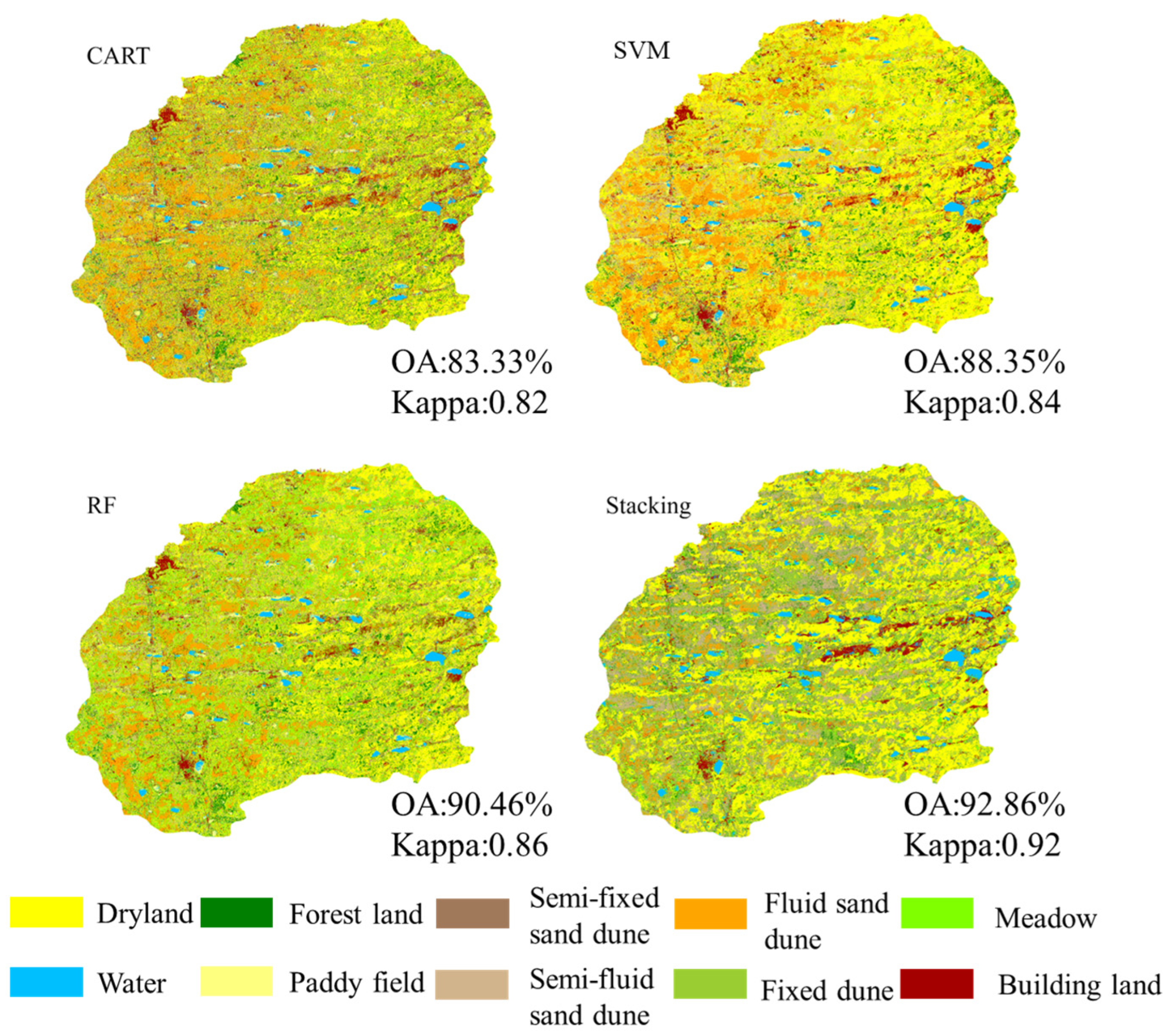
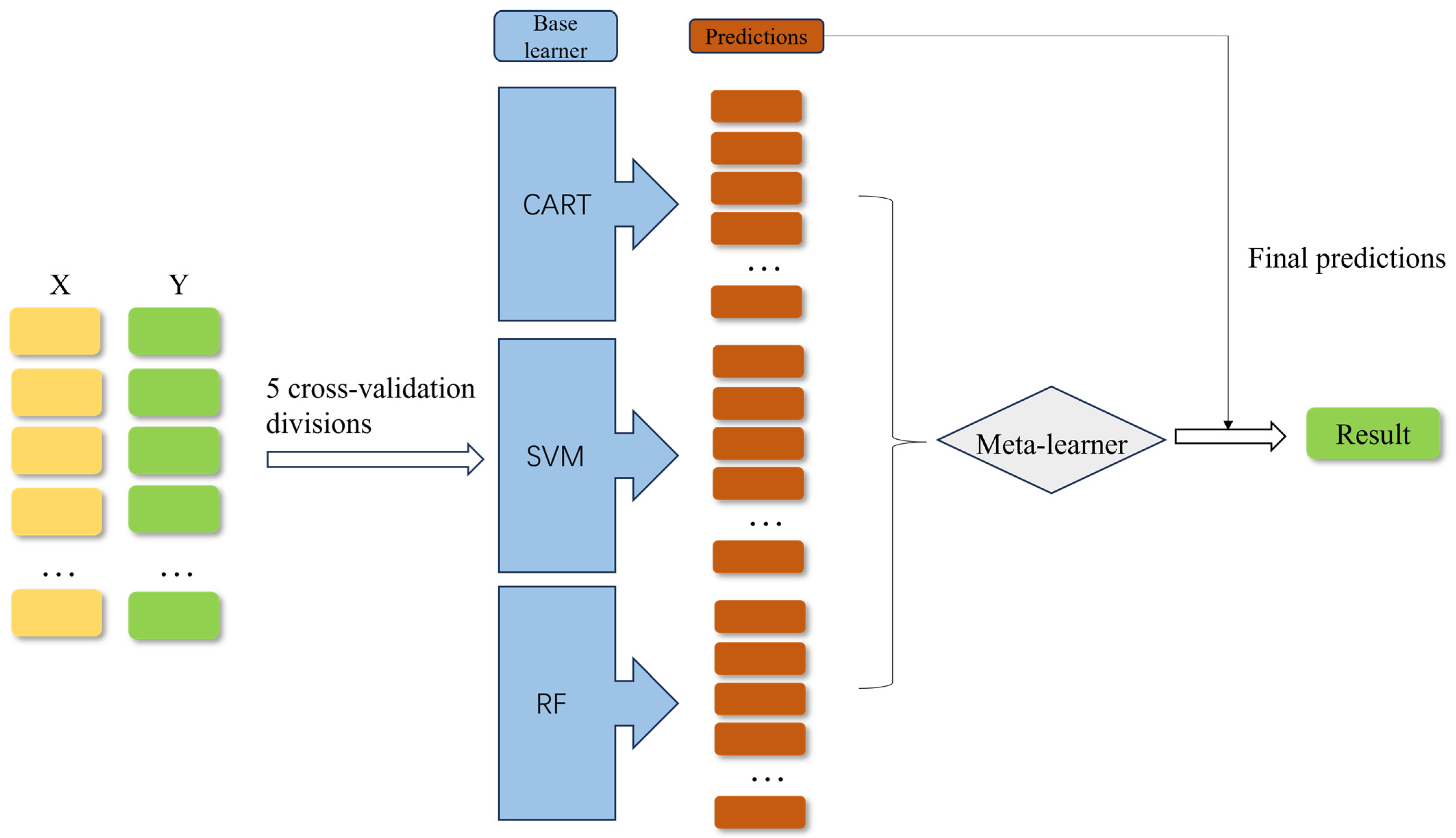
For the final land cover classification, this study applied the Stacking algorithm, a representative ensemble learning approach. The method was generalized into a two-stage classifier consisting of first-stage “base learners” (BLs) and a second-stage “meta-learner” (ML). To enhance the classification diversity that can be positively correlated to accuracy, three classical machine learning algorithms available on the GEE platform, including Classification and Regression Trees (CARTs), Support Vector Machines (SVMs), and Random Forests (RFs), were selected as the base learners (Figure 2), which are described in detail in the Supplementary Materials. In terms of meta-learner selection, prior studies have suggested that Random Forest can consistently outperform simple logistic regression classifiers. Accordingly, Random Forest was employed as the ML component within the Stacking framework [11]. Comparative experiments demonstrated that the Stacking algorithm substantially outperformed the three individual classifiers (CART, SVM, and RF), achieving an overall accuracy of 92.86% with a Kappa coefficient of 0.92 (Figure 3). The optimal hyperparameters of the basic learner are all determined by the random search method [35].

2.4. Quantification and Trend Analysis of Ecosystem Services

This study applied the CASA model to estimate NPP and employed the InVEST model to simulate the spatio-temporal variations in five key ESs within the study area: Habitat Quality (HQ), Carbon Stock (C), Water Yield (WY), and Soil Retention (SR). The specific parameters of the InVEST model and CASA model are in the Supplementary Materials. To further analyze the spatio-temporal dynamics and drivers of ESs, non-parametric trend estimation methods (Theil–Sen regression and Mann–Kendall tests) were integrated with the Geodetector model. Statistical analyses were performed using R to characterize the spatio-temporal evolution and interrelations of ESs. We will conduct a trend analysis on the quantified ESs (the details will be explained in the Supplementary Materials).
(1)
Net Primary Productivity (NPP)
Defined as the net photosynthetic carbon fixation of vegetation after plant respiration, NPP reflects the total carbon assimilated [36,37]. The improved CASA model, widely adopted at the regional scale [38], was applied using ENVI 5.6 software. The monthly mean temperature, precipitation, total solar radiation, and NDVI for different vegetation types were used as inputs to estimate the regional NPP from 2000 to 2024. The formula is as follows:
N P P x , t = A P A R x , t × ε x , t ,
where NPP(x,t) denotes the NPP at location x and time t, expressed in grams of carbon per square meter (gC/m2); APAR(x,t) represents the absorbed photosynthetically active radiation at location x and time t, measured in megajoules per square meter (MJ/m2); and ε(x,t) indicates the light use efficiency at location x and time t.
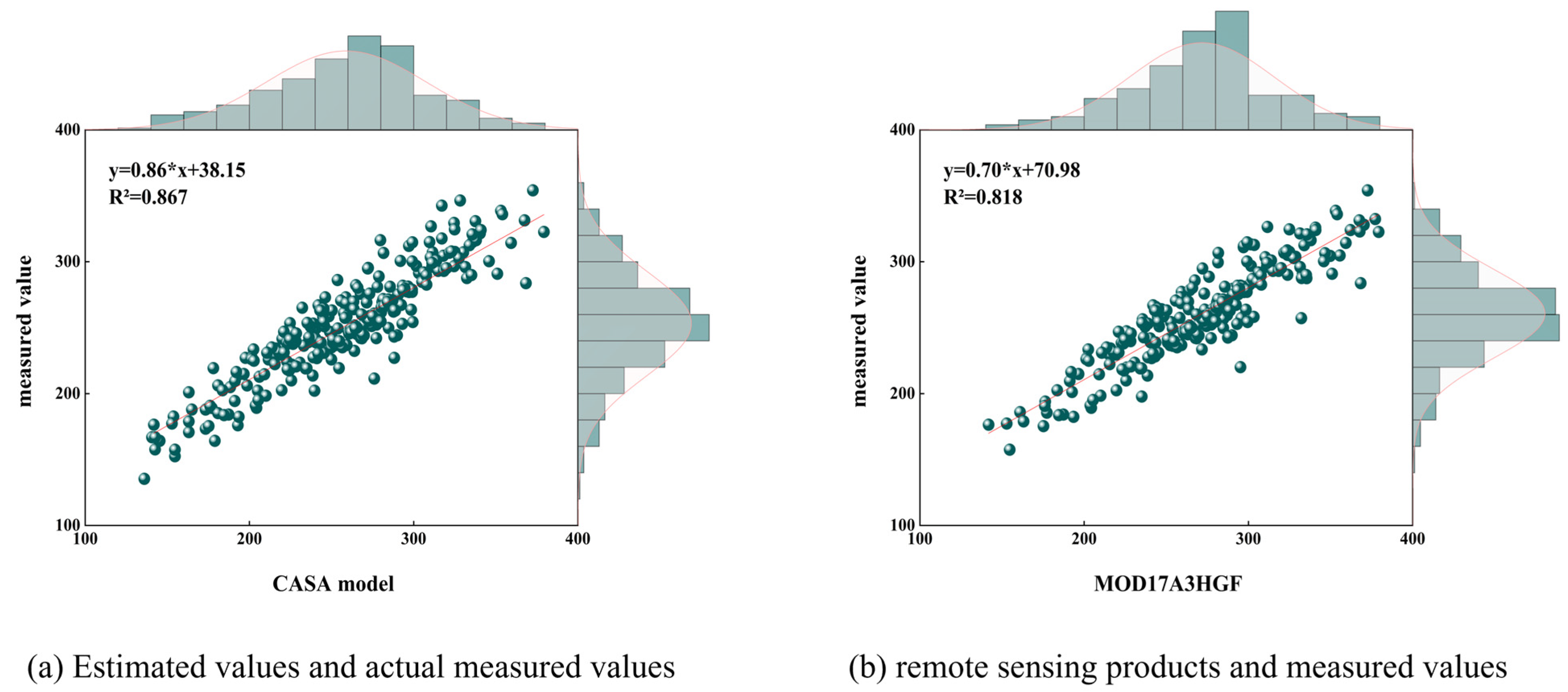
The 2024 field measurements and the MOD17A3HGF NPP dataset were used to validate the CASA model for estimating vegetation NPP within the study area [39]. A total of 27 field plots were established (Figure 1), with five 1 m × 1 m quadrats arranged at each location according to vegetation type, topography, elevation, and soil characteristics. In October, the field samples for NPP validation were collected. The harvested plants were transferred to gauze nets, litter was washed with water, and samples were oven-dried at 85 °C to a constant weight to determine biomass. The biomass values were subsequently multiplied by a conversion factor of 0.45 to estimate NPP (gC/m2) [40]. The validation results demonstrated a highly significant positive correlation between NPP estimated by the improved CASA model and observed values, with R2 = 0.867 (Figure 4a), confirming the model’s reliability. Further comparison revealed that NPP derived from the MOD17A3HGF dataset was also strongly correlated with the measured NPP in the study area (R2 = 0.818; Figure 4b). These findings further demonstrate the feasibility of applying the CASA model for regional NPP estimation.
(2)
Habitat Quality (HQ)
Habitat Quality modeling is inherently spatial and is estimated by integrating land use and land cover data with threats to species habitats. The Habitat Quality module evaluates regional habitats by incorporating parameters such as LUCC data, stress factors, and associated weights, thereby quantifying the current HQ of the study area. The index can be calculated based on landscape sensitivity and the intensity of external threats [41]. The formula is expressed as follows:
Q x j = H j 1 D x j z D x j Z + k z ,
where Qxj denotes the Habitat Quality index for grid cell x within land cover type j; Hj represents the habitat suitability of land cover type j; Dxj represents the total stress level experienced by grid cell x within land cover type j; K is the semi-saturation coefficient, with a default value of 0.05; and z is the normalization constant, set to 0.5 [42,43].
(3)
Carbon Stock (C)
Ecosystem Carbon Stock consists of four components: aboveground biomass, belowground biomass, soil carbon, and dead organic matter [44,45,46]. Aboveground biomass includes all aboveground organic matter, such as tree trunks, branches, and foliage. Belowground biomass refers to the living roots of plants beneath the soil surface. Soil organic matter represents the organic fraction of soil, whereas dead organic matter includes fallen branches, leaves, and dead trees. The formula is defined as follows [33,47]:
C t o t a l = C a b o v e + C b e l o w + C s o i l + C d e a d ,
where Ctotal denotes the total Carbon Stock within the study area, Cabove represents the aboveground biomass Carbon Stock, Cbelow indicates the belowground biomass Carbon Stock, Csoil denotes the soil Carbon Stock, and Cdead denotes the dead organic Carbon Stock.
(4)
Water Yield (WY)
The InVEST model incorporates factors such as topography and soil permeability variations to estimate Water Yield, thereby improving the reliability of its results [33,48]. This model allows flexible parameter adjustment and provides robust spatial outputs. In this study, the Water Yield module of the InVEST model was applied based on the Budyko water–heat coupling balance hypothesis, expressed as follows:
Y x = 1 A E T x P x × P x ,
where Y(x) denotes the annual Water Yield (mm) for each grid cell x within the watershed, AET(x) represents the annual actual evapotranspiration (mm) for grid cell x, and P(x) represents the annual precipitation (mm) for grid cell x.
(5)
Soil Retention (SR)
Soil Retention was quantified using the sediment transport ratio module of the InVEST model. The Universal Soil Loss Equation (USLE) was applied to calculate actual soil erosion and potential soil loss (RKLS), with Soil Retention (SR) determined as follows [49]:
S R = R K L S U S L E ,
U S L E = R × L S × P × C ,
R K L S = R × K × L S ,
where USLE denotes the annual average soil erosion rate (t∙hm−2); R denotes the rainfall erosion factor; K denotes the soil erodibility factor; SAND denotes the percentage of sand particles in the soil; SILT denotes the percentage of silt particles in the soil; OC represents the percentage of organic matter in the soil; LS represents the slope length and steepness factor; C represents the cover and management factor; and P represents the protective measures factor.

2.5. Analysis of Driving Factors

Geodetector models are widely applied to detect spatial heterogeneity and its driving factors, allowing the investigation of the impact levels of individual factors and their interactions. Compared with traditional regression models, they provide distinct analytical benefits. It developed a parameter-optimized Geodetector framework that automatically identifies the optimal discretization method and the number of classes for continuous data, thereby improving the precision of spatial analysis [50]. In this study, 10 factors, including land use type (X1), NDVI (X2), slope (X3), DEM (X4), precipitation (X5), temperature (X6), population density (X7), sand content (X8), silt content (X9), and clay content (X10), were employed to quantitatively analyze the drivers of ESs in the study area from 2000 to 2024. By applying the factor detection, and interaction detection of the Optimal Parameter Geodetector (OPGD), the underlying factors influencing the changes in functions such as NPP within the study area from 2000 to 2024 were systematically revealed. Due to the potential endogeneity issue between NDVI as a driving factor and NPP, we will provide a detailed explanation in the Supplementary Materials.
Differentiation and factor detection: detecting the spatial differentiation of Y; and the extent to which the detection of a certain factor X explains the spatial differentiation of attribute Y. Measured by the q value, the expression is as follows:
q = 1 h = 1 L N h σ h 2 N σ 2 = 1 S S W S S T ,
S S W = h = 1 L N h σ h 2 , S S T = N σ 2
In the formula, h = 1,… L represents the Strata of the variable Y or the factor X, that is, classification or partitioning. N h and N represent the number of units in layer h and the entire region, respectively. σ h 2 and σ 2 are the variances of the Y values of layer h and the entire region, respectively. SSW and SST are, respectively, the sum of variances within the layer and the total sum of squares in the entire are. The range of q is [0, 1]. The larger the value, the more obvious the spatial discrimination of Y.
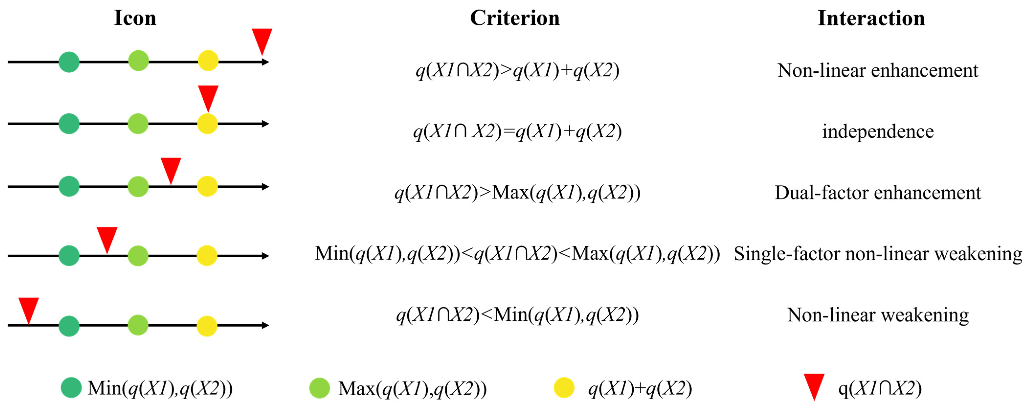
Interaction detection: Identify the interaction between different risk factors Xs, that is, evaluate whether the combined action of factors X1 and X2 will increase or decrease the explanatory power for the dependent variable Y, or whether the influence of these factors on Y is independent of each other (Figure 5).

2.6. Identification of ESs Trade-Offs and Synergies

This study uses Spearman correlation coefficient to quantify the spatial correlation between ecosystem services, as a fundamental tool for identifying trade-off (negative correlation) and synergy (positive correlation) statistical patterns. It should be clearly pointed out that statistical correlation reflects the co-occurrence of spatial patterns, but it is not directly equivalent to causal relationships or specific ecological mechanisms. To avoid overinterpretation, this article will first report these statistical patterns in the results Section 3.4, and then in the discussion Section 4.3, we will combine the land use dynamics, water resource conditions, vegetation characteristics, and policy background of the study area to explore in-depth the potential ecological and geographical processes behind these key patterns, in order to establish a logical connection between statistical laws and systematic processes [51]. This method was selected for its robustness in handling non-linear relationships and resistance to the influence of extreme values, while not requiring data normalization. It has been widely used in ES trade-off and synergy studies. Data processing, correlation analysis, and result visualization were conducted in R, with correlation matrices primarily visualized using the corrplot package. The formula is expressed as follows:
R a , b = 1 6 Σ d a b 2 n 3 n ,
t = R × n 2 1 R 2 ,
where a and b represent the ESs of different categories; R(a,b) denotes the correlation coefficient between a and b; dab represents the rank difference between a and b; n is the sample size; and t is the test value. R(a,b) > 0 corresponds to a positive correlation, signifying synergistic interactions, with larger values representing stronger synergies. Conversely, R(a,b) < 0 indicates a negative correlation, reflecting the trade-offs between ESs, with smaller values corresponding to stronger trade-offs. Based on the long-term changes in ESs, a pixel-by-pixel spatial analysis was conducted to calculate the correlation coefficients between ES pairs within each grid cell, thereby identifying spatial trade-offs and synergies. Employing this pixel-level approach to quantify the trade-offs and synergies in long-term change datasets further strengthens the analysis of overall ES interactions (Table 2).

3. Results

3.1. Spatial and Temporal Dynamics of Land Use

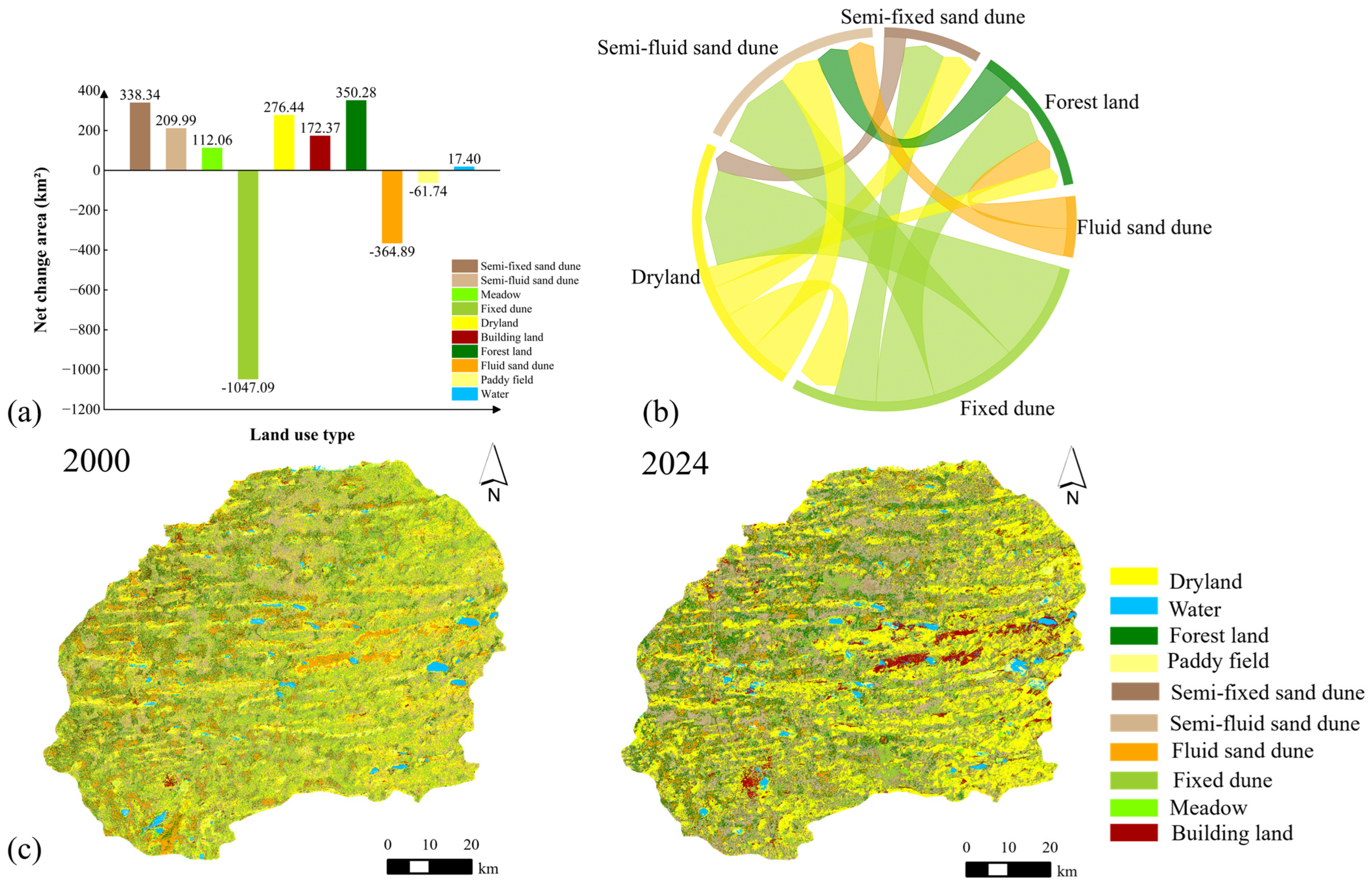
The results of the net change in land use types (Figure 6a) indicate that semi-fixed sand dunes and forest land experienced the most substantial area increases, with net gains of 338.34 km2 and 350.28 km2, respectively. In contrast, fixed sand dunes exhibited the most pronounced decline, with a net reduction of 1047.09 km2. Additionally, the areas of dryland, semi-fluid land, building land, meadow land, and water have all increased to varying extents, whereas fluid sand dunes and paddy fields have seen reductions in area.
The chord plot analysis based on the transition matrix (Figure 6b) reveals that the transformation of fixed sand dunes is the predominant process of land use change during the study period, with the area undergoing transformation comprising 27% of the total transformation area. The primary types of fixed sand dunes have transitioned to dryland and semi-fluid sand dunes, with additional transfers occurring to other land use categories. Regarding spatial distribution patterns (Figure 6c), from 2000 to 2024, the expansion of semi-fixed sand dunes and forest land was predominantly concentrated in the western region of the study area. Conversely, the reduction in fixed sand dunes exhibits a global characteristic, demonstrating a significant trend of area decline across the entire study area, which underscores the extensive spatial nature of this land use change.

3.2. The Spatio-Temporal Distribution Pattern of Ecosystem Services

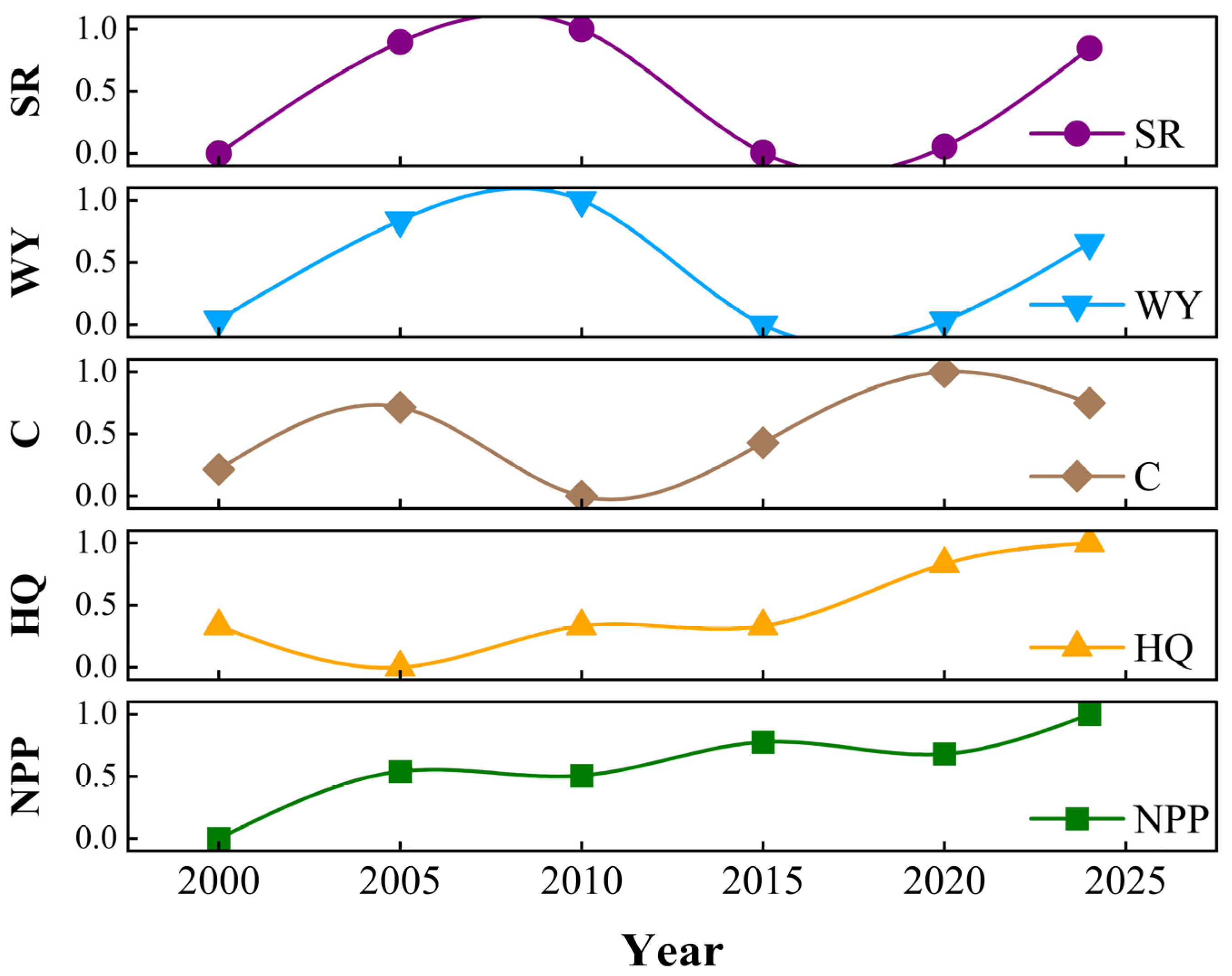
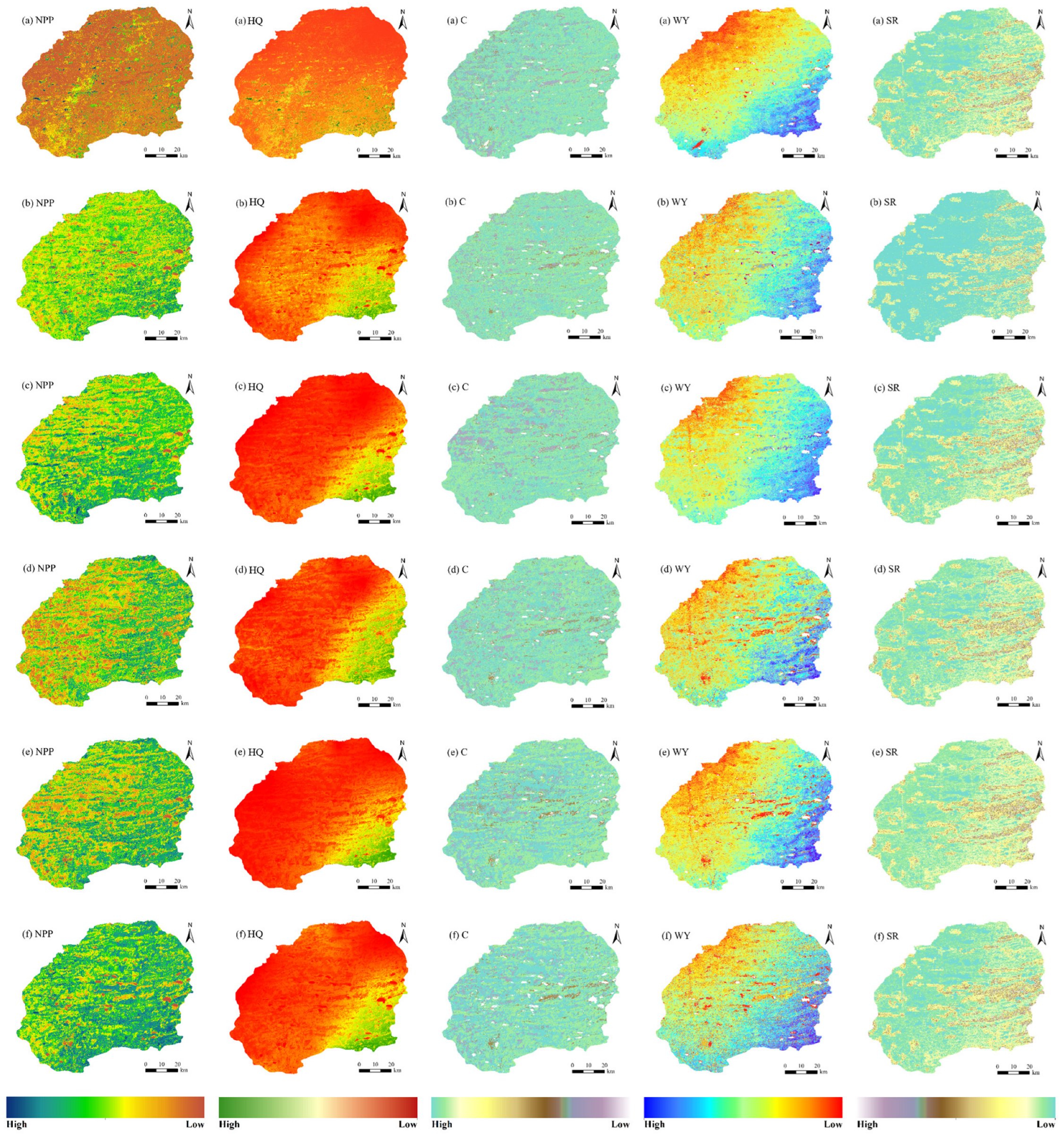
From 2000 to 2024, the changes in ecosystem services in the study area showed significant spatio-temporal differentiation (Figure 7 and Figure 8). In terms of the time dimension, NPP, HQ and SR generally show an upward trend and C remains relatively stable, while WY generally declines. These overall trends exhibit obvious heterogeneity in space. The results of Theil–Sen slope estimation and the Mann–Kendall trend test further reveal that NPP has significantly increased in the 69.22% region. HQ significantly improved in 66.43% of the regions, and the improved areas were mainly concentrated in the east. WY shows a downward trend in 53.22% of the southern region. Although SR rose overall, the spatial differentiation was significant. The areas with significant improvement were concentrated in the northeastern part, while 40.85% of the areas still showed a downward trend.

3.3. Analysis of Factors Influencing ESs

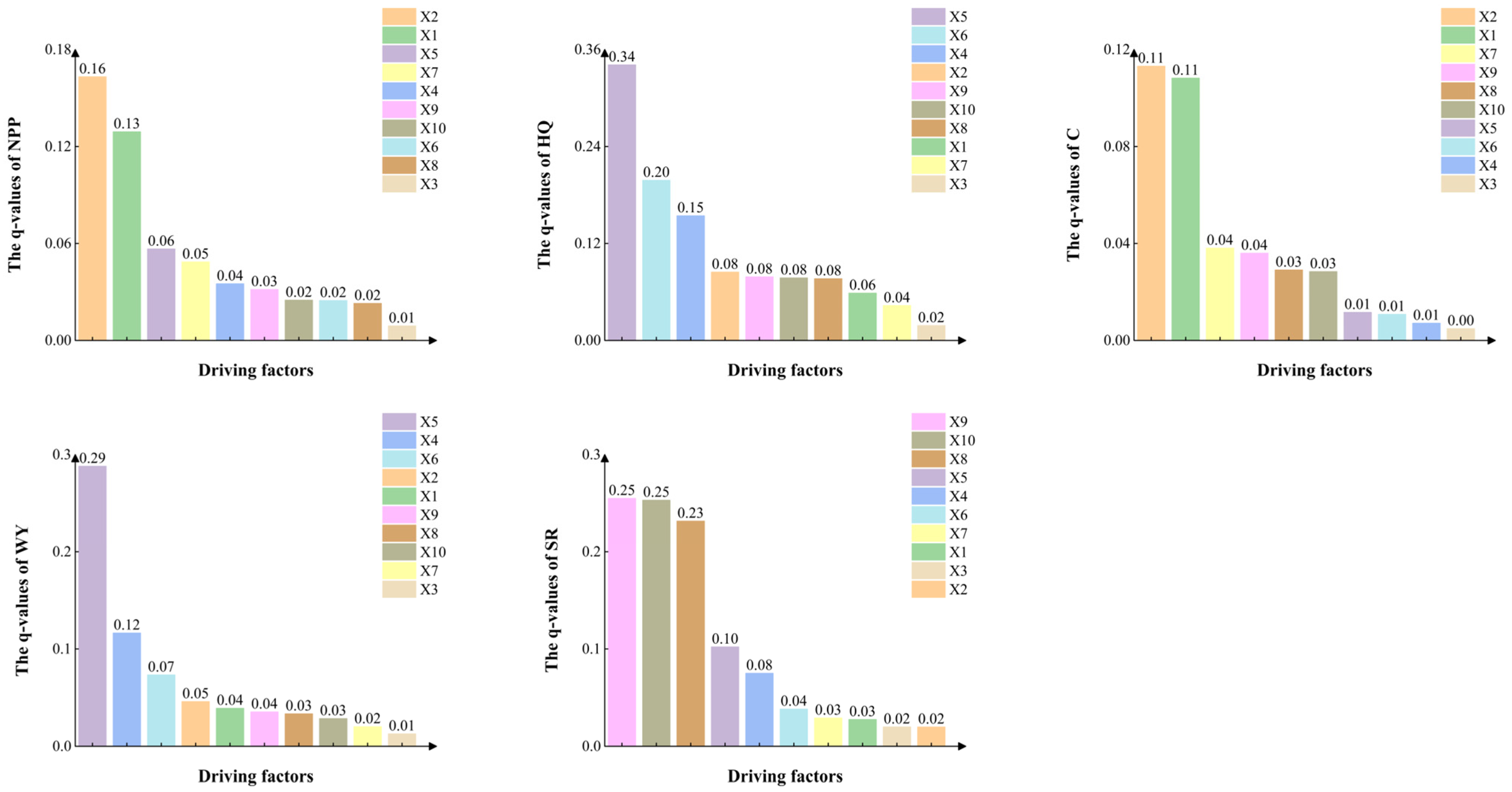
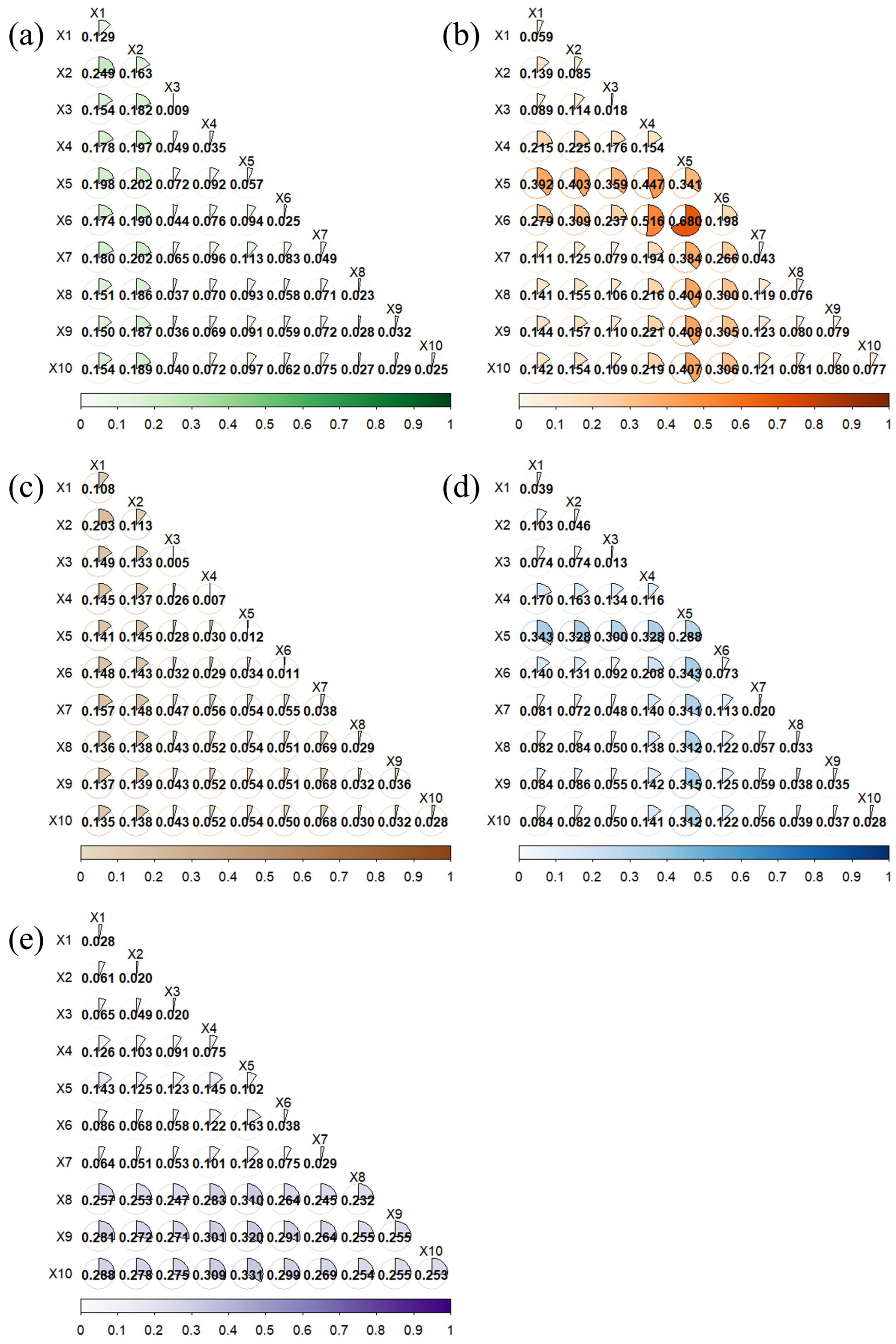
Analyze the driving effects of single factors and interaction factors on ecosystem services through geographic detectors. The results show that the dominant driving factors of different ecosystem services vary significantly (Figure 9 shows the explanatory power of single factors from high to low), and the explanatory power of interaction factors is generally greater than that of single factors (Figure 10). As the dominant factors, NDVI and land use type have an explanatory power of more than 25% for both NPP and C. For HQ and WY, the precipitation factor is dominant, with an explanatory power of over 30% for both. The explanatory power of soil texture (silt content q = 0.25, clay content q = 0.25, sand content q = 0.23) for SR accounts for 70%. However, slope and population density have relatively weak explanatory power for all services, with an overall explanatory power of less than 10%.
Under the influence of the interaction factor, the interaction between X1 and X2 shows a two-factor enhancement in the explanatory power of NPP and C, and both are greater than 25%. The interaction between X5 and X6 has a non-linear enhancement effect on HQ. X5, X6 and other factors all show a two-factor enhancement, while the other two factors are non-linear weakened. Among them, the interactions between X6 and X4 and between X5 and X6 are the strongest, and the degree of interaction is all above 50%. The interaction between X5 and X1 has a non-linear enhancement effect on WY, with an interaction exceeding 30%. X5 and the other factors all show a synergistic enhancement. The interactions of X8, X9, and X10 with all other factors have a significantly greater impact on SR than the pairwise interactions. The interactions with other factors, from largest to smallest, are X10 > X9 > X8, showing a two-factor enhancement.

3.4. Trade-Offs and Synergies in ESs

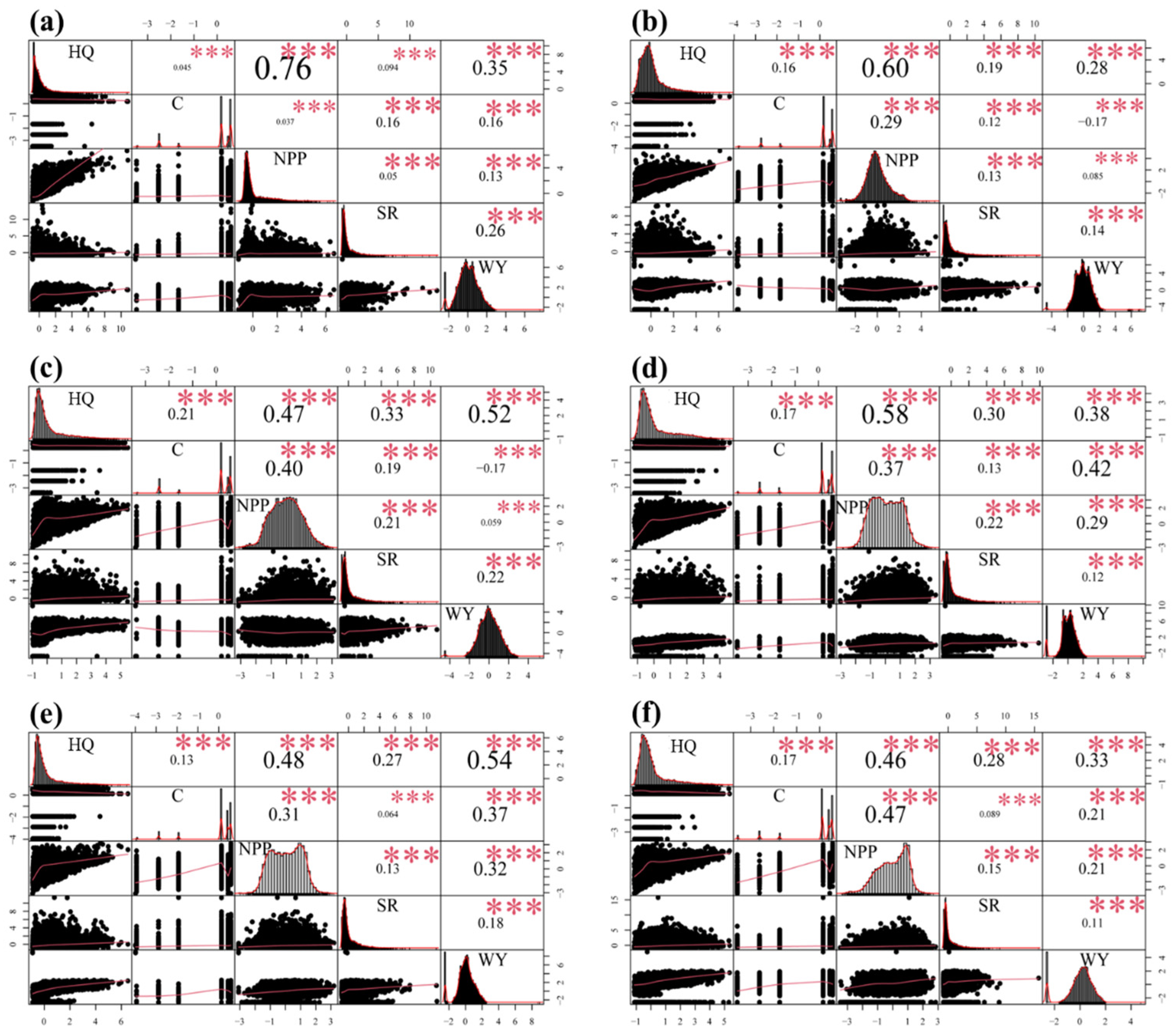
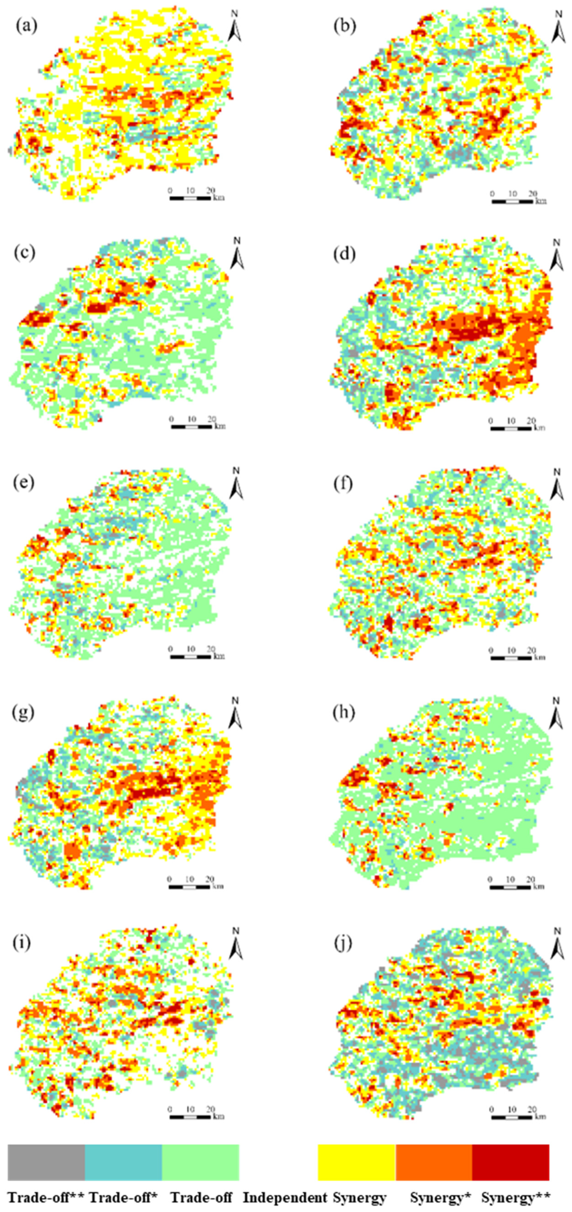
From 2000 to 2024, there was a significant positive correlation (p < 0.01) among ecosystem services (ESs) within the study area. In terms of timing, NPP and HQ, as well as HQ and WY, mostly maintain synergy in most years. The synergy between NPP and C, as well as HQ and SR, was particularly significant in certain years, such as 2005, 2010, 2015, and 2024. Only C and WY showed a weak trade-off (index 0.17) in 2005 and 2010, and then turned to synergy. Among them, 2015 was the peak year for the collaborative relationship of multiple pairs of ESs. After that, the overall synergy strengthened, and the six pairs of ESs showed strong synergy.
Spatially, the relationships among ecosystem services show significant heterogeneity (Figure 11). The eastern region mainly presents two patterns: NPP–WY and C–WY show strong synergy, while HQ–SR, NPP–SR and C–SR mostly show trade-off relationships. Overall, SR–WY is mainly collaborative, and C–HQ also shows overall collaboration and remains stable in the east. The remaining services (HQ–WY, C–NPP, NPP–HQ) show a weak trade-off overall, but there are significant synergy areas locally (Figure 12).

4. Discussion

4.1. Patterns of Change in ESs

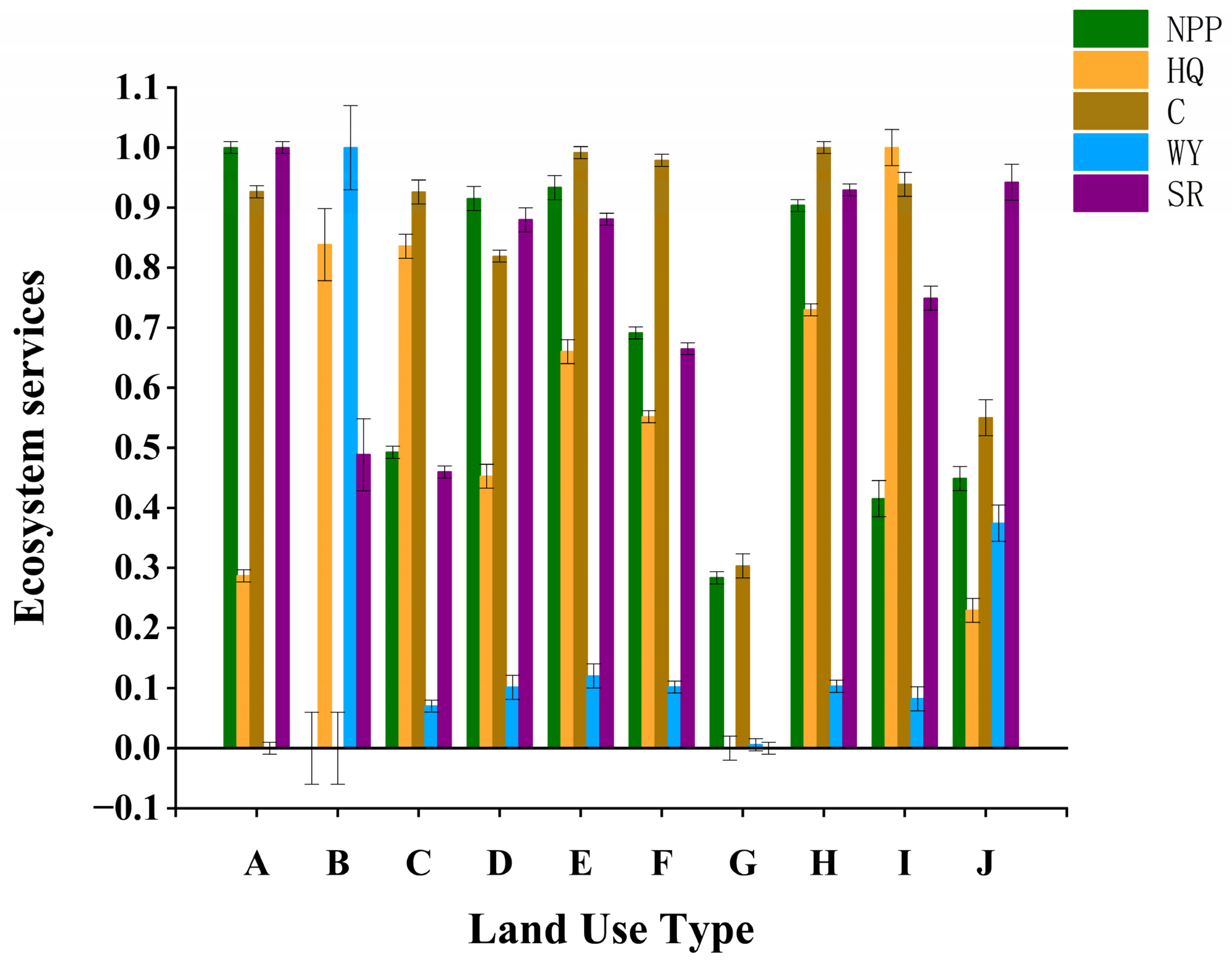
From 2000 to 2024, the ecosystem services of the Horqin Sandy Land ecotone exhibited complex characteristics typical of an ecological–agricultural interface (Figure 13). Driven by land use transformation, the overall increases in NPP, SR, HQ, and C sharply contrast with the decline in WY. The differing capacities of various land use types to provide essential ecosystem services intensified the cumulative effects of these disparities during the study period. The key findings of this study regarding ESs in the alternating dune-meadow regions of Horqin were highly consistent with those of multiple recent investigations across arid, semi-arid, and ecologically fragile zones. For instance, it reported an increasing trend in NPP from 2000 to 2020 in the Hexi Corridor, consistent with the results of this study [52]. The rise in NPP can be attributed primarily to the expansion of dryland and semi-fixed sand dunes. Concurrently, the forested areas that have experienced the most significant increase also contribute substantially to cumulative biomass. This phenomenon highlights the synergistic impact of agricultural practices and ecological engineering on enhancing productivity.
Similarly, the findings of this study of an overall increase in SR are aligned with the conclusions of research conducted in the Hexi Corridor and other ecologically fragile regions in northern China [53,54]. The essence of SR enhancement is the large-scale transformation of SR values from extremely low fluid and fixed sand dunes to semi-fixed sand dunes, dryland, or meadow. This process facilitates the transition from an erosion “source” to a “sink” by improving surface coverage and the capacity for root consolidation [55].
However, despite widespread regional vegetation restoration, trade-offs among key ESs persist, primarily driven by alterations in water cycle processes. The present findings and those of the Hexi study [52] indicate a declining trend in WY. The explanation for this phenomenon is that the substantial increase in dryland, forest land, and meadows consists of land types characterized by relatively low water production capacity per unit area. In contrast, the water area associated with high-water-producing types remains relatively stable. Consequently, the overall shift in land use toward low-water-producing types directly contributes to the decline in regional WY. In semi-arid regions, the total evapotranspiration of forest ecosystems, including canopy interception, understory transpiration, and vegetation transpiration, frequently exceeds precipitation inputs [55,56]. In areas characterized by limited and uneven precipitation, trees extract groundwater through deep root systems, further intensifying water loss. On the other hand, the widespread expansion of dryland areas, primarily in the east and southeast, requires intensive agricultural irrigation. This artificial diversion of water for irrigation has amplified surface runoff and groundwater extraction, significantly reducing the water resources available for ecosystem storage and gradual release. The combined effects of water consumption from afforestation and dryland expansion have altered the regional water cycle. Along with findings from other northern regions, evidence from this study consistently documented a decline in WY [55,57]. Consequently, land use change has a profound impact on water conservation functions by directly modifying surface energy balance (via evapotranspiration) and water fluxes, including infiltration, runoff generation, and groundwater extraction.
The findings of Mao et al. [58] for the Beijing–Tianjin–Hebei region indicated that the increases in HQ and C can be primarily driven by vegetation restoration, which is consistent with the present study. These results largely reflect the universal pattern of ES under shared policy drivers, such as the Grain-for-Green Program, ecological engineering initiatives, and climate change. Structural transformations in LUCC during the “degradation–restoration” process regulate the synergistic and trade-off patterns of ESs. The improvement in HQ and C is closely related to the restoration of natural vegetation: The area of meadow land and forest land with the highest supply capacity of HQ has significantly increased, directly enhancing habitat suitability. The change in C reflects the characteristics of sandy land. The area of high carbon storage types such as fixed sand dunes has decreased, and most of them have been transformed into semi-fixed sand dunes and forest land with medium carbon storage, achieving a stable transformation of the carbon pool from “high-density storage” to “higher density and also featuring living vegetation carbon sinks”, thereby supporting the overall growth of carbon storage.
Our findings indicate that the expansion of dryland in the Horqin Sandy Land contributes to an increase in NPP; however, its extremely low water production capacity significantly exacerbates the imbalance of water resources. Contrary to the prevailing belief that forests serve as the primary carbon sinks, this study reveals that the fixed and semi-fixed sand dunes in Horqin represent important soil carbon reservoirs. Consequently, the fixation of sandy land during the ecological restoration process not only enhances vegetation carbon sinks but also induces morphological changes and potential risks to the original soil carbon pool. Furthermore, a spatial differentiation exists between NPP and SR: The eastern region primarily relies on dryland, whereas the western ecological restoration area is dependent on forest and grass vegetation.

4.2. Driving Mechanisms of Trends in ES Changes

To elucidate the regulatory mechanisms underlying trade-offs and synergies among ESs in the Horqin Sandy Land, this study quantified their spatio-temporal dynamics and identified key drivers. The results indicated that the interactions between multiple factors significantly enhanced explanatory power for the spatial differentiation of ESs, as evidenced by elevated q-values. This finding aligned with the results of [59]. ESs arise from complex coupling processes between natural elements and human activities, with the influence of individual factors amplified or moderated through synergistic or antagonistic interactions with other spatially heterogeneous variables, resulting in a comprehensive non-linear dynamic pattern. The spatial differentiation of NPP is mainly driven by the interaction between land use types and NDVI, and its explanatory power is on the rise. This result is the same as the analysis in Section 4.1: Land use types (such as dryland and forest land) determine the upper limit of NPP, while NDVI reflects the actual vegetation growth status. The combination of the two explains the significant spatial heterogeneity of NPP under the same land use types. It is proved that the improvement in vegetation productivity depends on the combination of appropriate land use and good vegetation conditions [60]. HQ is mainly dominated by precipitation and its interaction with temperature. As key climatic variables, these two drivers directly or indirectly shape vegetation productivity, structural complexity, and species distribution, thereby influencing habitat suitability and connectivity. This pattern corroborates the findings from the study [61]. The substantial increase in the interaction q-values between these factors during 2000–2020 further suggests that climatic variability and its combined effects increasingly dominated HQ dynamics. The C formation was predominantly governed by the interaction between land use and NDVI but also strongly affected by population density and slope gradient. Land use change shapes carbon pool structures and sequestration potential, whereas vegetation biomass dynamics driven by NDVI determine carbon distribution. Rising population density has intensified land use pressures, with slope gradients further amplifying disturbance effects in vulnerable regions. Together, these drivers constitute a “human–geography” composite pressure system, exposing carbon stocks to multi-dimensional stresses [62,63]. HQ is more constrained by a relatively stable climate background, while C is more directly exposed to rapidly changing human land use activities. Precipitation is the fundamental climatic factor explaining the spatial patterns of WY and SR. However, its explanatory power shows a downward trend in WY, indicating that, in the context of climate warming, WY no longer solely depends on precipitation. The moderating effects of land use types and other factors on WY are becoming increasingly important [53]. In arid and semi-arid regions under climate warming and drying trends, prolonged drought stress intensifies vegetation degradation and soil crusting, and reduces infiltration, thereby weakening the responsiveness of hydrological processes to precipitation and diminishing WY. SR was largely driven by precipitation, with rainfall intensifying water erosion risks through enhanced runoff and scouring, which is consistent with the findings from the Loess Plateau [64]. Soil texture also emerged as a decisive factor, with clay-rich soils contributing to aggregate stability and erosion resistance, whereas sandy soils were more susceptible to erosion. For SR, the interaction between precipitation and soil types has become the most explanatory factor, and its influence continues to increase. This indicates that the erosive force of precipitation needs to be combined with erosive soil to be transformed into actual soil erosion risks. The expansion of erosive areas such as semi-fixed sand dunes may have enhanced this effect. In conclusion, the spatial differentiation of ESs in the Horqin Sandy Land is driven by the coupling of multiple factors. Climatic factors provide the fundamental environmental background and resource input; land use directly reflects the transformation of the surface structure and ecological processes by human activities. The dynamics of vegetation are an important link for realizing ecological functions. The interaction among these factors is the core mechanism for the complex spatial differences presented by regional ecosystem services [65].

4.3. Trade-Offs and Synergies Between ESs

From 2000 to 2024, the various ecosystem services in the Horqin Sandy Land were dominated by collaborative relationships, and there was a significant positive correlation generally (p < 0.01), especially in years such as 2015 and 2020 when the benefits of ecological engineering were remarkable. This indicates that regional ecological restoration measures have, in most cases, led to the simultaneous improvement of multiple benefits. However, limited and specific trade-off relationships also exist and exhibit obvious temporal fluctuations and spatial heterogeneity. This pattern reveals that the ES correlation is not static but a complex network that dynamically adjusts with climate fluctuations, policy intervention stages, and the evolution of land use patterns. In the initial phase of the study area (2000), vegetation coverage in the Horqin Sandy Land was relatively low. The restoration of vegetation markedly enhanced HQ, establishing a synergistic relationship between NPP and HQ. However, in subsequent stages, the simplification of artificial vegetation and potential landscape fragmentation from excessive afforestation in certain localities led to a gradual weakening of this synergy. This shift underscores the necessity for adjustments in ecological governance policies. Following 2021, the Horqin Sandy Land has fostered a combination of engineering governance and natural restoration, which has positively contributed to the restoration and regulation of this ecosystem service. Similarly, the synergy between NPP and C in specific years (2005, 2010, 2015, and 2024) highlighted the critical role of vegetation in carbon sequestration. Since 2000, the Horqin Sandy Land has progressively undertaken ecological initiatives, including the conversion of farmland to forest and meadow, as well as artificial afforestation. These efforts have markedly increased the NPP of vegetation. The ongoing accumulation of vegetation biomass has concurrently improved the C capacity of the region, illustrating the synergy between vegetation restoration and Carbon Stock functions driven by policy measures. This development aligns closely with China’s strategic objective of enhancing the carbon sink capacity of ecosystems in the context of the “dual carbon” goals. However, the interannual variability in these synergies (e.g., NPP–C synergy was not significant in all years) reflects the regulatory influence of climate change, such as precipitation variability, or phased human interventions. The ongoing implementation and cumulative effects of the fifth phase of the Three-North Shelter Forest Program and the “Double Million Mu” comprehensive management project in the Left Wing Rear Banner of Horqin have led to a synergistic peak in HQ and WY services in 2010 and 2020. The significant increase in vegetation coverage has not only directly enhanced HQ but also improved the soil’s capacity for water retention and runoff regulation. This observation underscores the synergistic relationship between these two key ecosystem services, driven by major ecological policies. In 2015, WY exhibited significant synergies with HQ, C, and NPP. The implementation of ecological projects in Inner Mongolia, such as the Natural Forest Conservation Program and the Beijing–Tianjin Sandstorm Source Control Project, has substantially enhanced the hydrological regulation and carbon stock of vegetation [66,67].
In human-dominated landscapes, land use transitions and conservation policies constitute major disturbances, altering ES interrelationships. Land use transformations disrupt ecological equilibrium by modifying landscape connectivity and patch structures, thereby intensifying ESs trade-offs. Conversely, conservation policies foster synergies by optimizing landscape patterns and promoting cooperative ES relationships [68]. Compared with synergies, significant trade-offs were limited, with only weak negative correlations observed between C and WY in 2005 and 2010. In the initial stage of vegetation restoration, the forested area within the study region experienced a continuous increase. The early artificial forests, predominantly composed of water-intensive species such as poplar trees, contributed to rising C. However, the heightened water consumption associated with these trees may have diminished regional runoff, thereby creating a trade-off between C and WY services. At the regional scale, SR and WY generally exhibited weak synergies, with topography and vegetation cover favoring soil conservation and indirectly supporting water conservation. However, a dominant weak trade-off between NPP and SR was identified in eastern regions, likely associated with intensive agricultural development. The encroachment of cultivated land into natural vegetation was linked to SR decline.
Studies have indicated that, while ES interactions can exhibit certain interannual fluctuations, such as changes in the strength of synergies, with carbon–water trade-offs occurring only in certain years, no fundamental directional reversal has occurred in the long term. This relative stability suggests that regional ecosystems maintain a degree of resilience. Long-term observations have further revealed that, while NPP–WY trade-offs and synergies present cyclical fluctuations due to climatic variability, they remain embedded within core associative patterns [69,70]. Regional variations in ES association patterns were equally pronounced. Within the Belt and Road region, driven by restoration policies, HQ consistently exhibited stable synergies with both C and SR, consistent with findings from ecologically comparable regions. This concordance underscores the universality of ecological policies in enhancing synergies. However, the high spatial heterogeneity also highlights the fragility of local systems, which depends strongly on the alignment of human management strategies with natural endowments. The dynamic changes in the correlation of ecosystem services in the Horqin Sandy Land from 2000 to 2024 illustrate a significant transformation in ecological governance policies, evolving from an initial focus on “single sand prevention and control” to a framework of “multi-functional collaborative governance of the ecosystem.” Notably, the transition from a trade-off relationship to a synergistic interaction between C and WY, along with the ongoing enhancement of synergy between vegetation NPP and C, reflects the interplay between policy optimization and the ecosystem’s positive feedback mechanisms. These findings provide a crucial foundation for advancing the coordinated enhancement of multiple ecosystem services during ecological restoration efforts in arid and semi-arid regions.

5. Conclusions

From 2000 to 2024, significant changes occurred in land use and the ecosystem in the study area. The fixed sand dunes have decreased on a large scale, mainly transforming into dryland and semi-fluid sand dunes. At the same time, the area of semi-fixed sand dunes and forests increased. This process of land use change has profoundly influenced ecosystem services. Ecosystem services present a pattern of overall improvement but significant internal differences. NPP and HQ have significantly improved, while WY has declined. The spatial patterns of changes in various services are not consistent. Analysis shows that the main driving factors of different services are different. Among them, NDVI and land use type have prominent influences on NPP and C, precipitation is the key factor of WY, and soil type is the key factor of SR. When two factors interact, their explanatory power is usually stronger than that of any single factor. During this period, the interaction relationships among various ecosystem services have undergone dynamic evolution, moving from relatively simple to complex. The synergy among some services has strengthened, while that among others has weakened, reflecting the internal dynamic adjustment of ecosystem services. In conclusion, ecological management in the study area needs to comprehensively consider the complex relationships among different services and their main driving factors to support the balance between sustainable land use and ecological protection.

Supplementary Materials

The following supporting information can be downloaded at: https://www.mdpi.com/article/10.3390/land15020299/s1, Figure S1: (a) Changes in land use types in the study area, (b) Sankey diagram of the conversion of each land use type from 2000 to 2024; Figure S2: Spatial distribution of land use types in the study area; Figure S3: Trends in ecosystem services in the study area (2000–2024) ((a) NPP, (b) HQ, (c) C, (d) WY, and (e) SR); Figure S4: Trends in spatially averaged ecosystem services ((a) NPP, (b) HQ, (c) C, (d) WY, and (e) SR) in the study area (2000–2024); Figure S5: The q values of ecosystem services for different land types with and without NDVI; Figure S6: Results of driving factor interaction detection; Table S1: Threshold information of each band for sample points without land class change; Table S2: Changes in land use area; Table S3: Transition matrix 2000–2024; Table S4: CASA model Parameters; Table S5: Threat source parameters; Table S6: Threat sensitivity parameters; Table S7: The carbon density for each land use type in the study area (mg C/hm2); Table S8: Water yield module parameters; Table S9: Cover management factor (C) and conservation practice factor (P); Table S10: Classification of Mann–Kendall test results; Table S11: Changes in ecosystem service trends; Table S12: The temporal variation in q values with and without NDVI; Table S13: Table group driving factors Q value; Table S14: Impact factor classification method and number of tiers.

Author Contributions

Conceptualization, X.G., Y.B. and T.L.; Formal analysis, X.G.; Methodology, X.G., Y.B. and T.L.; Visualization, X.G., Y.B. and V.P.S.; Writing—original draft, X.G.; Writing—review and editing, Y.B., L.H. and T.L.; Funding acquisition, L.H., L.D. and T.L.; Data curation, Y.B., S.L., J.S. and V.P.S.; Resources, Y.B. and T.L.; Supervision, Y.B., L.H., L.D., S.L., J.S. and T.L. All authors have read and agreed to the published version of the manuscript.

Funding

This study was supported by the National Natural Science Foundation of China [Grant Nos. 52439004, 52309021, and 52109022]; the National Key Research and Development Program of China [Grant No. 2024YFF1306302]; the Inner Mongolia Autonomous Region Science and Technology Leading Talent Team [Grant No. 2022LJRC0007]; the Inner Mongolia Agricultural University Basic Research Project [Grant Nos. BR221012, BR221204 and BR251018]; the First-class Academic Subjects Special Research Project of the Education Department of Inner Mongolia Autonomous Region (Grant Nos. YLXKZX-NND-010 and YLXKZX-NND-028); the Ministry of Education of China Innovative Research Team [Grant No. IRT_17R60]; the Chinese Ministry of Science and Technology Innovative Research Team in Priority Areas [Grant No. 2015RA4013].

Data Availability Statement

Data will be made available on request.

Acknowledgments

We would like to thank the anonymous reviewers for their valuable commentsand suggestions.

Conflicts of Interest

The authors declare that they have no known competing financial interests or personal relationships that could have appeared to influence the work reported in this paper.

Abbreviations

The following abbreviations are used in this manuscript:
ESsEcosystem Services
NPPNet Primary Productivity
HQHabitat Quality
CCarbon Stock
WYWater Yield
SRSoil Retention

References

  1. Li, C.; Zheng, H.; Li, S.; Chen, X.; Li, J.; Zeng, W.; Liang, Y.; Polasky, S.; Feldman, M.W.; Ruckelshaus, M.; et al. Impacts of Conservation and Human Development Policy across Stakeholders and Scales. Proc. Natl. Acad. Sci. USA 2015, 112, 7396–7401. [Google Scholar] [CrossRef] [PubMed]
  2. Baldassini, P.; Sans, G.C.; Segura, D.A.; Conde, C.; Paruelo, J.M. Mapping Cropping Systems and Their Effects on Ecosystem Functioning and Services in the Argentine Pampas. Agric. Ecosyst. Environ. 2024, 369, 109027. [Google Scholar] [CrossRef]
  3. Assandri, G.; Bogliani, G.; Pedrini, P.; Brambilla, M. Beautiful Agricultural Landscapes Promote Cultural Ecosystem Services and Biodiversity Conservation. Agric. Ecosyst. Environ. 2018, 256, 200–210. [Google Scholar] [CrossRef]
  4. Cardinale, B.J.; Duffy, J.E.; Gonzalez, A.; Hooper, D.U.; Perrings, C.; Venail, P.; Narwani, A.; Mace, G.M.; Tilman, D.; Wardle, D.A.; et al. Biodiversity Loss and Its Impact on Humanity. Nature 2012, 486, 59–67. [Google Scholar] [CrossRef]
  5. Niu, W.; Ding, J.; Fu, B.; Zhao, W.; Eldridge, D. Global Effects of Livestock Grazing on Ecosystem Functions Vary with Grazing Management and Environment. Agric. Ecosyst. Environ. 2025, 378, 109296. [Google Scholar] [CrossRef]
  6. Straubinger, C.; Reisch, C.; Poschlod, P. The Influence of Historical Management on the Vegetation and Habitat Properties of Semi-Dry Grassland. Agric. Ecosyst. Environ. 2021, 320, 107587. [Google Scholar] [CrossRef]
  7. Dang, L.; Zhao, F.; Teng, Y.; Teng, J.; Zhan, J.; Zhang, F.; Liu, W.; Wang, L. Scale Dependency of Trade-Offs/Synergies Analysis of Ecosystem Services Based on Bayesian Belief Networks: A Case of the Yellow River Basin. J. Environ. Manage. 2025, 375, 124410. [Google Scholar] [CrossRef]
  8. Hu, Z.; Wang, S.; Bai, X.; Luo, G.; Li, Q.; Wu, L.; Yang, Y.; Tian, S.; Li, C.; Deng, Y. Changes in Ecosystem Service Values in Karst Areas of China. Agric. Ecosyst. Environ. 2020, 301, 107026. [Google Scholar] [CrossRef]
  9. Chen, Z.; Huang, M.; Zhu, D.; Altan, O. Integrating Remote Sensing and a Markov-FLUS Model to Simulate Future Land Use Changes in Hokkaido, Japan. Remote Sens. 2021, 13, 2621. [Google Scholar] [CrossRef]
  10. Tamiminia, H.; Salehi, B.; Mahdianpari, M.; Quackenbush, L.; Adeli, S.; Brisco, B. Google Earth Engine for Geo-Big Data Applications: A Meta-Analysis and Systematic Review. ISPRS J. Photogramm. Remote Sens. 2020, 164, 152–170. [Google Scholar] [CrossRef]
  11. Cai, Y.; Li, X.; Zhang, M.; Lin, H. Mapping Wetland Using the Object-Based Stacked Generalization Method Based on Multi-Temporal Optical and SAR Data. Int. J. Appl. Earth Obs. Geoinf. 2020, 92, 102164. [Google Scholar] [CrossRef]
  12. Zhang, M.; Lin, H.; Long, X.; Cai, Y. Analyzing the Spatiotemporal Pattern and Driving Factors of Wetland Vegetation Changes Using 2000-2019 Time-Series Landsat Data. Sci. Total Environ. 2021, 780, 146615. [Google Scholar] [CrossRef]
  13. Clinton, N.; Yu, L.; Gong, P. Geographic Stacking: Decision Fusion to Increase Global Land Cover Map Accuracy. ISPRS J. Photogramm. Remote Sens. 2015, 103, 57–65. [Google Scholar] [CrossRef]
  14. Healey, S.P.; Cohen, W.B.; Yang, Z.; Kenneth Brewer, C.; Brooks, E.B.; Gorelick, N.; Hernandez, A.J.; Huang, C.; Joseph Hughes, M.; Kennedy, R.E.; et al. Mapping Forest Change Using Stacked Generalization: An Ensemble Approach. Remote Sens. Environ. 2018, 204, 717–728. [Google Scholar] [CrossRef]
  15. Dennedy-Frank, P.J.; Muenich, R.L.; Chaubey, I.; Ziv, G. Comparing Two Tools for Ecosystem Service Assessments Regarding Water Resources Decisions. J. Environ. Manage. 2016, 177, 331–340. [Google Scholar] [CrossRef] [PubMed]
  16. Zhang, D.; Wang, J.; Wang, Y.; Xu, L.; Zheng, L.; Zhang, B.; Bi, Y.; Yang, H. Is There a Spatial Relationship between Urban Landscape Pattern and Habitat Quality? Implication for Landscape Planning of the Yellow River Basin. Int. J. Environ. Res. Public Health 2022, 19, 11974. [Google Scholar] [CrossRef]
  17. Wu, C.; Chen, K.; E, C.; You, X.; He, D.; Hu, L.; Liu, B.; Wang, R.; Shi, Y.; Li, C.; et al. Improved CASA Model Based on Satellite Remote Sensing Data: Simulating Net Primary Productivity of Qinghai Lake Basin Alpine Grassland. Geosci. Model Dev. 2022, 15, 6919–6933. [Google Scholar] [CrossRef]
  18. Xiao, J.; Song, F.; Su, F.; Shi, Z.; Song, S. Quantifying the Independent Contributions of Climate and Land Use Change to Ecosystem Services. Ecol. Indic. 2023, 153, 110411. [Google Scholar] [CrossRef]
  19. Andersson, E.; McPhearson, T.; Kremer, P.; Gomez-Baggethun, E.; Haase, D.; Tuvendal, M.; Wurster, D. Scale and Context Dependence of Ecosystem Service Providing Units. Ecosyst. Serv. 2015, 12, 157–164. [Google Scholar] [CrossRef]
  20. Cord, A.F.; Bartkowski, B.; Beckmann, M.; Dittrich, A.; Hermans-Neumann, K.; Kaim, A.; Lienhoop, N.; Locher-Krause, K.; Priess, J.; Schröter-Schlaack, C.; et al. Towards Systematic Analyses of Ecosystem Service Trade-Offs and Synergies: Main Concepts, Methods and the Road Ahead. Ecosyst. Serv. 2017, 28, 264–272. [Google Scholar] [CrossRef]
  21. Luo, Y.; Guo, X.; Lü, Y.; Zhang, L.; Li, T. Combining Spatiotemporal Interactions of Ecosystem Services with Land Patterns and Processes Can Benefit Sensible Landscape Management in Dryland Regions. Sci. Total Environ. 2024, 909, 168485. [Google Scholar] [CrossRef] [PubMed]
  22. Chen, T.; Peng, L.; Liu, S.; Wang, Q. Spatio-Temporal Pattern of Net Primary Productivity in Hengduan Mountains Area, China: Impacts of Climate Change and Human Activities. Chin. Geogr. Sci. 2017, 27, 948–962. [Google Scholar] [CrossRef]
  23. Wang, J.; Li, X.; Christakos, G.; Liao, Y.; Zhang, T.; Gu, X.; Zheng, X. Geographical Detectors-based Health Risk Assessment and Its Application in the Neural Tube Defects Study of the Heshun Region, China. Int. J. Geogr. Inf. Sci. 2010, 24, 107–127. [Google Scholar] [CrossRef]
  24. Ye, S.; Ren, S.; Song, C.; Cheng, C.; Shen, S.; Yang, J.; Zhu, D. Spatial Patterns of County-Level Arable Land Productive-Capacity and Its Coordination with Land-Use Intensity in Mainland China. Agric. Ecosyst. Environ. 2022, 326, 107757. [Google Scholar] [CrossRef]
  25. Huang, S.; Xiao, L.; Zhang, Y.; Wang, L.; Tang, L. Interactive Effects of Natural and Anthropogenic Factors on Heterogenetic Accumulations of Heavy Metals in Surface Soils through Geodetector Analysis. Sci. Total Environ. 2021, 789, 147937. [Google Scholar] [CrossRef]
  26. Wang, S.; Zhang, L.; Zhang, H.; Han, X.; Zhang, L. Spatial–Temporal Wetland Landcover Changes of Poyang Lake Derived from Landsat and HJ-1A/B Data in the Dry Season from 1973–2019. Remote Sens. 2020, 12, 1595. [Google Scholar] [CrossRef]
  27. Griffiths, J.R.; Schindler, D.E.; Armstrong, J.B.; Scheuerell, M.D.; Whited, D.C.; Clark, R.A.; Hilborn, R.; Holt, C.A.; Lindley, S.T.; Stanford, J.A.; et al. Performance of Salmon Fishery Portfolios across Western North America. J. Appl. Ecol. 2014, 51, 1554–1563. [Google Scholar] [CrossRef] [PubMed]
  28. Qiao, X.; Gu, Y.; Zou, C.; Wang, L.; Luo, J.; Huang, X. Trade-Offs and Synergies of Ecosystem Services in the Taihu Lake Basin of China. Chin. Geogr. Sci. 2018, 28, 86–99. [Google Scholar] [CrossRef]
  29. Duan, H.; Wang, T.; Xue, X.; Yan, C. Dynamic Monitoring of Aeolian Desertification Based on Multiple Indicators in Horqin Sandy Land, China. Sci. Total Environ. 2019, 650, 2374–2388. [Google Scholar] [CrossRef]
  30. Jia, X.; Bai, X.; Liu, C.; Zhao, C.; Shao, M.; Pan, Y. Differences in Plant Water Use between Check-Dam Land and Slope Land on the Loess Plateau: Significance for Vegetation Restoration. Agric. Ecosyst. Environ. 2024, 362, 108849. [Google Scholar] [CrossRef]
  31. Li, Y.; Li, F.Y.; Shi, C.; Wang, H.; Wu, L.; Wang, Y.; Minggagud, H. Precipitation and Grazing Intensity Jointly Shape Plant Compensatory Growth and Productivity in a Semi-Arid Steppe Ecosystem. Agric. Ecosyst. Environ. 2025, 393, 109834. [Google Scholar] [CrossRef]
  32. Zhou, J.; Jia, L.; Menenti, M.; Liu, X. Optimal Estimate of Global Biome—Specific Parameter Settings to Reconstruct NDVI Time Series with the Harmonic ANalysis of Time Series (HANTS) Method. Remote Sens. 2021, 13, 4251. [Google Scholar] [CrossRef]
  33. Zhang, W.; Fan, Y.; Qiao, Q.; Shao, G.; Zhang, M.; Lei, S.; Han, Y. Delineating Ecological Restoration Zoning Integrating Functional and Structural Models in Horqin Sandy Land, China. Forests 2025, 16, 1616. [Google Scholar] [CrossRef]
  34. Yan, X.; Li, J.; Smith, A.R.; Yang, D.; Ma, T.; Su, Y. Rapid Land Cover Classification Using a 36-Year Time Series of Multi-Source Remote Sensing Data. Land 2023, 12, 2149. [Google Scholar] [CrossRef]
  35. Bochenek, R. Random Search Optimization Approach for Highly Multi-Modal Nonlinear Problems. Adv. Eng. Softw. 2005, 36, 504–517. [Google Scholar] [CrossRef]
  36. Peng, J.; Shen, H.; Wu, W.; Liu, Y.; Wang, Y. Net Primary Productivity (NPP) Dynamics and Associated Urbanization Driving Forces in Metropolitan Areas: A Case Study in Beijing City, China. Landsc. Ecol 2016, 31, 1077–1092. [Google Scholar] [CrossRef]
  37. Bai, W.; Fang, Y.; Zhou, M.; Xie, T.; Li, L.; Zhang, W.-H. Heavily Intensified Grazing Reduces Root Production in an Inner Mongolia Temperate Steppe. Agric. Ecosyst. Environ. 2015, 200, 143–150. [Google Scholar] [CrossRef]
  38. Zheng, Z.; Zhu, W.; Zhang, Y. Seasonally and Spatially Varied Controls of Climatic Factors on Net Primary Productivity in Alpine Grasslands on the Tibetan Plateau. Glob. Ecol. Conserv. 2020, 21, e00814. [Google Scholar] [CrossRef]
  39. Liu, L.; Guan, J.; Zheng, J.; Wang, Y.; Han, W.; Liu, Y. Cumulative Effects of Drought Have an Impact on Net Primary Productivity Stability in Central Asian Grasslands. J. Environ. Manag. 2023, 344, 118734. [Google Scholar] [CrossRef] [PubMed]
  40. Zhang, M.; Yuan, N.; Lin, H.; Liu, Y.; Zhang, H. Quantitative Estimation of the Factors Impacting Spatiotemporal Variation in NPP in the Dongting Lake Wetlands Using Landsat Time Series Data for the Last Two Decades. Ecol. Indic. 2022, 135, 108544. [Google Scholar] [CrossRef]
  41. Yohannes, H.; Soromessa, T.; Argaw, M.; Dewan, A. Spatio-Temporal Changes in Habitat Quality and Linkage with Landscape Characteristics in the Beressa Watershed, Blue Nile Basin of Ethiopian Highlands. J. Environ. Manage. 2021, 281, 111885. [Google Scholar] [CrossRef]
  42. Pan, R.; Yan, J.; Ling, H.; Xia, Q. Exploring Multi-Scale Synergies, Trade-Offs, and Driving Mechanisms of Ecosystem Services in Arid Regions: A Case Study of the Ili River Valley. Land 2025, 14, 2166. [Google Scholar] [CrossRef]
  43. Terrado, M.; Sabater, S.; Chaplin-Kramer, B.; Mandle, L.; Ziv, G.; Acuña, V. Model Development for the Assessment of Terrestrial and Aquatic Habitat Quality in Conservation Planning. Sci. Total Environ. 2016, 540, 63–70. [Google Scholar] [CrossRef]
  44. Nan, G.; Wang, J.; Han, L.; He, X.; Jiang, W.; Ma, J. Does Slope Cropland to Natural and Artificial Conversion Change Patterns of Soil Moisture–Carbon Trade-Offs in Time and Depth on the Water-Scarce Loess Plateau, China? Agric. Ecosyst. Environ. 2025, 385, 109583. [Google Scholar] [CrossRef]
  45. Tölgyesi, C.; Kelemen, A.; Bátori, Z.; Kiss, R.; Hábenczyus, A.A.; Havadtői, K.; Varga, A.; Erdős, L.; Frei, K.; Tóth, B.; et al. Maintaining Scattered Trees to Boost Carbon Stock in Temperate Pastures Does Not Compromise Overall Pasture Quality for the Livestock. Agric. Ecosyst. Environ. 2023, 351, 108477. [Google Scholar] [CrossRef]
  46. Zafar, Z.; Zubair, M.; Zha, Y.; Mehmood, M.S.; Rehman, A.; Fahd, S.; Nadeem, A.A. Predictive Modeling of Regional Carbon Storage Dynamics in Response to Land Use/Land Cover Changes: An InVEST-Based Analysis. Ecol. Inf. 2024, 82, 102701. [Google Scholar] [CrossRef]
  47. Xu, C.; Zhang, Q.; Yu, Q.; Wang, J.; Wang, F.; Qiu, S.; Ai, M.; Zhao, J. Effects of Land Use/Cover Change on Carbon Storage between 2000 and 2040 in the Yellow River Basin, China. Ecol. Indic. 2023, 151, 110345. [Google Scholar] [CrossRef]
  48. Wang, H.; Huang, L.; Zhang, H.; Fu, Y.; Guo, W.; Jiao, X.; Zhou, H.; Zhu, Y. Development of a Decision Framework for River Health and Water Yield Ecosystem Service in Watershed. J. Hydrol. 2023, 623, 129773. [Google Scholar] [CrossRef]
  49. Marques, S.M.; Campos, F.S.; David, J.; Cabral, P. Modelling Sediment Retention Services and Soil Erosion Changes in Portugal: A Spatio-Temporal Approach. ISPRS Int. J. Geo-Inf. 2021, 10, 262. [Google Scholar] [CrossRef]
  50. Song, Y.; Wang, J.; Ge, Y.; Xu, C. An Optimal Parameters-Based Geographical Detector Model Enhances Geographic Characteristics of Explanatory Variables for Spatial Heterogeneity Analysis: Cases with Different Types of Spatial Data. GIScience Remote Sens. 2020, 57, 593–610. [Google Scholar] [CrossRef]
  51. Qu, S.; Jiang, Y.; Gao, J.; Cao, Q.; Wang, L.; Zhang, Y.; Huang, F. Spatial–Temporal Evolution and Driving Factors of Ecosystem Services Trade-Offs and Synergies in Karst Areas from a Geospatial Perspective. Land Degrad. Dev. 2024, 35, 3448–3460. [Google Scholar] [CrossRef]
  52. Xiao, S.; Xia, H.; Zhai, J.; Jin, D.; Gao, H. Trade-off and Synergy Relationships and Driving Factor Analysis of Ecosystem Services in the Hexi Region. Remote Sens. 2024, 16, 3147. [Google Scholar] [CrossRef]
  53. Wang, X.; Wu, J.; Liu, Y.; Hai, X.; Shanguan, Z.; Deng, L. Driving Factors of Ecosystem Services and Their Spatiotemporal Change Assessment Based on Land Use Types in the Loess Plateau. J. Environ. Manag. 2022, 311, 114835. [Google Scholar] [CrossRef]
  54. Yang, S.; Zhao, W.; Liu, Y.; Wang, S.; Wang, J.; Zhai, R. Influence of Land Use Change on the Ecosystem Service Trade-Offs in the Ecological Restoration Area: Dynamics and Scenarios in the Yanhe Watershed, China. Sci. Total Environ. 2018, 644, 556–566. [Google Scholar] [CrossRef]
  55. Wang, H.; Wang, W.J.; Liu, Z.; Wang, L.; Zhang, W.; Zou, Y.; Jiang, M. Combined Effects of Multi-Land Use Decisions and Climate Change on Water-Related Ecosystem Services in Northeast China. J. Environ. Manag. 2022, 315, 115131. [Google Scholar] [CrossRef]
  56. Bernal, S.; Lupon, A.; Ribot, M.; Sabater, F.; Martí, E. Riparian and In-Stream Controls on Nutrient Concentrations and Fluxes in a Headwater Forested Stream. Biogeosciences 2015, 12, 1941–1954. [Google Scholar] [CrossRef]
  57. Jiang, W.; Fu, B.; Gao, G.; Lv, Y.; Wang, C.; Sun, S.; Wang, K.; Schüler, S.; Shu, Z. Exploring Spatial-Temporal Driving Factors for Changes in Multiple Ecosystem Services and Their Relationships in West Liao River Basin, China. Sci. Total Environ. 2023, 904, 166716. [Google Scholar] [CrossRef]
  58. Mao, B.; Wang, X.; Liao, Z.; Miao, Y.; Yan, S. Spatiotemporal Variations and Tradeoff-Synergy Relations of Ecosystem Services under Ecological Water Replenishment in Baiyangdian Lake, North China. J. Environ. Manag. 2023, 343, 118229. [Google Scholar] [CrossRef] [PubMed]
  59. Chen, Z.; Wei, K.; Hu, L.; Yi, C.; Liu, S. Spatiotemporal Variation and Driving Forces of Carbon Storage in the Fuhe River Basin, China. Sci. Rep. 2025, 15, 30224. [Google Scholar] [CrossRef] [PubMed]
  60. Tang, C.; Li, J.; Zhou, Z.; Zeng, L.; Zhang, C.; Ran, H. How to Optimize Ecosystem Services Based on a Bayesian Model: A Case Study of Jinghe River Basin. Sustainability 2019, 11, 4149. [Google Scholar] [CrossRef]
  61. Zeng, X.; Hu, Z.; Chen, A.; Yuan, W.; Hou, G.; Han, D.; Liang, M.; Di, K.; Cao, R.; Luo, D. The Global Decline in the Sensitivity of Vegetation Productivity to Precipitation from 2001 to 2018. Glob. Change Biol. 2022, 28, 6823–6833. [Google Scholar] [CrossRef] [PubMed]
  62. Tao, J.; Dong, J.; Zhang, Y.; Yu, X.; Zhang, G.; Cong, N.; Zhu, J.; Zhang, X. Elevation-Dependent Effects of Growing Season Length on Carbon Sequestration in Xizang Plateau Grassland. Ecol. Indic. 2020, 110, 105880. [Google Scholar] [CrossRef]
  63. Zong, R.; Wang, Z.; Wu, Q.; Guo, L.; Lin, H. Characteristics of Carbon Emissions in Cotton Fields under Mulched Drip Irrigation. Agric. Water Manag. 2020, 231, 105992. [Google Scholar] [CrossRef]
  64. Feng, Q.; Zhao, W.; Hu, X.; Liu, Y.; Daryanto, S.; Cherubini, F. Trading-off Ecosystem Services for Better Ecological Restoration: A Case Study in the Loess Plateau of China. J. Clean. Prod. 2020, 257, 120469. [Google Scholar] [CrossRef]
  65. Gudmundsson, L.; Greve, P.; Seneviratne, S.I. The Sensitivity of Water Availability to Changes in the Aridity Index and Other Factors—A Probabilistic Analysis in the Budyko Space. Geophys. Res. Lett. 2016, 43, 6985–6994. [Google Scholar] [CrossRef]
  66. Pang, Y.; Wu, B.; Cao, Y.; Jia, X. Spatiotemporal Changes in Terrestrial Water Storage in the Beijing-Tianjin Sandstorm Source Region from GRACE Satellites. Int. Soil Water Conserv. Res. 2020, 8, 295–307. [Google Scholar] [CrossRef]
  67. Tang, X.; Zhao, X.; Bai, Y.; Tang, Z.; Wang, W.; Zhao, Y.; Wan, H.; Xie, Z.; Shi, X.; Wu, B.; et al. Carbon Pools in China’s Terrestrial Ecosystems: New Estimates Based on an Intensive Field Survey. Proc. Natl. Acad. Sci. USA 2018, 115, 4021–4026. [Google Scholar] [CrossRef]
  68. Cimon-Morin, J.; Darveau, M.; Poulin, M. Fostering Synergies between Ecosystem Services and Biodiversity in Conservation Planning: A Review. Biol. Conserv. 2013, 166, 144–154. [Google Scholar] [CrossRef]
  69. Tian, Y.; Wang, S.; Bai, X.; Luo, G.; Xu, Y. Trade-Offs among Ecosystem Services in a Typical Karst Watershed, SW China. Sci. Total Environ. 2016, 566–567, 1297–1308. [Google Scholar] [CrossRef]
  70. Wei, C.; Su, K.; Jiang, X.; You, Y.; Zhou, X.; Yu, Z.; Chen, Z.; Liao, Z.; Zhang, Y.; Wang, L. Increase in Precipitation and Fractional Vegetation Cover Promote Synergy of Ecosystem Services in China’s Arid Regions—Northern Sand-Stabilization Belt. Front. Ecol. Evol. 2023, 11, 1116484. [Google Scholar] [CrossRef]
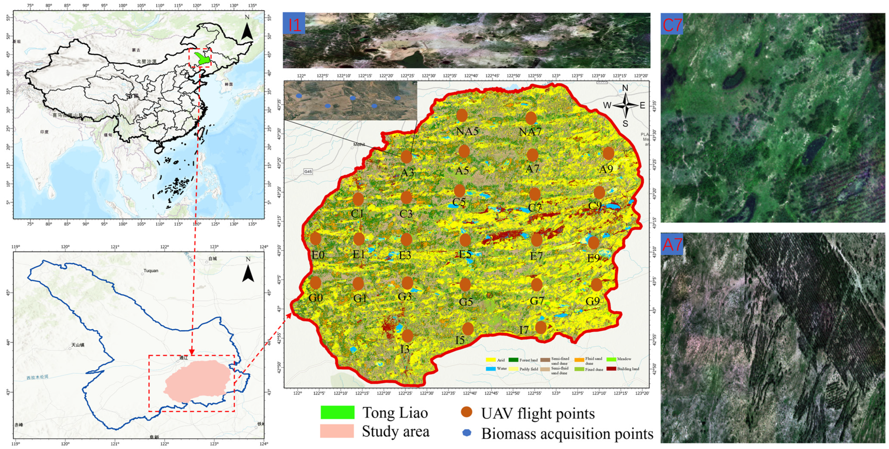
Figure 1. Study area.
Land 15 00299 g001
Figure 2. Principle of stacking algorithm.
Land 15 00299 g002
Figure 3. Comparison of land use methods.
Land 15 00299 g003
Figure 4. NPP estimate validation. (The asterisk (*) in the regression equations represents the multiplication sign).
Land 15 00299 g004
Figure 5. Types of interaction between two covariates.
Land 15 00299 g005
Figure 6. (a) Net change in land use from 2000 to 2024, (b) the main types of land use that will undergo transfer and change from 2000 to 2024, (c) spatial distribution of land use types from 2000 to 2024.
Land 15 00299 g006
Figure 7. Trends in average ecosystem services in the study area (2000–2024).
Land 15 00299 g007
Figure 8. Distribution of spatial patterns of Net Primary Productivity (NPP), Habitat Quality (HQ), Carbon Stock (C), Water Yield (WY), and Soil Retention (SR) (2000–2024).
Land 15 00299 g008
Figure 9. Ranking of the impact of single factor X1 (land use type), X2 (NDVI), X3 (slope), X4 (DEM), X5 (precipitation), X6 (temperature), X7 (population density), X8 (sand content), X9 (silt content), X10 (clay content) on ecosystem services.
Land 15 00299 g009
Figure 10. The impact of interactive detection factors (a) NPP, (b) HQ, (c) C, (d) WY and (e) SR on ecosystem services.
Land 15 00299 g010
Figure 11. (af) Index of ecosystem service trade-offs and synergies (2000–2024). HQ, C, NPP, SR, and WY represent Habitat Quality index, Carbon Stock, Net Primary Productivity, Soil Retention, and Water Yield, respectively. *** The size of changes with the magnitude of the correlation coefficient r.
Land 15 00299 g011
Figure 12. The trade-offs and synergies spatial relationship between different combinations of ecosystem services (a) SR–WY, (b) HQ–WY, (c) HQ–SR, (d) NPP–WY, (e) NPP–SR, (f) NPP–HQ, (g) C–WY, (h) C–SR, (i) C–HQ and (j) C–NPP. The strength of the trade-off and synergy relationship: * represents (0.01 < p < 0.05), ** represents (p < 0.01).
Land 15 00299 g012
Figure 13. The changes in ecosystem services under different land use types (A: dryland, B: water, C: forest land, D: paddy field, E: semi-fixed sand dune, F: semi-fluid dune, G: fluid sand dune, H: fixed dune, I: meadow, J: building land).
Land 15 00299 g013
Table 1. Description of the study data.
Impact FactorsSpatial ResolutionTime RangeData Sources and Related References
NDVI30 m2000–2024https://github.com/jiezhou87/HANTS-GEE/, accessed on 10 March 2025
Temperature1 km2000–2024https://www.resdc.cn/Default.aspx/, accessed on 20 July 2025
Precipitation1 km2000–2024https://www.resdc.cn/Default.aspx/, accessed on 20 July 2025
Population density1 km2000–2024https://landscan.ornl.gov/, accessed on 27 July 2025
Soil sand30 m2000–2024https://www.resdc.cn/Default.aspx/, accessed on 20 May 2025
Soil clay30 m2000–2024https://www.resdc.cn/Default.aspx/, accessed on 20 May 2025
Soil silt30 m2000–2024https://www.resdc.cn/Default.aspx/, accessed on 20 May 2025
DEM30 m2000–2024https://www.gscloud.cn/, accessed on 17 March 2025
NPP500 m2000–2024Google Earth Engine
Table 2. Judgment method for balancing synergy relationships.
Intensity of Trade-Off and Synergy RelationshipsBasis for Determination
Synergy **r > 0, p < 0.01
Synergy *r > 0.0.01 < p < 0.05
Synergyr > 0, 0.05 < p < 0.1
Independentp > 0.1
Trade-offr < 0, p < 0.01
Trade-off *r < 0, 0.01 < p < 0.05
Trade-off **r < 0, 0.05 < p < 0.1
The strength of the trade-off and synergy relationship: * represents (0.01 < p < 0.05), ** represents (p < 0.01).
Disclaimer/Publisher’s Note: The statements, opinions and data contained in all publications are solely those of the individual author(s) and contributor(s) and not of MDPI and/or the editor(s). MDPI and/or the editor(s) disclaim responsibility for any injury to people or property resulting from any ideas, methods, instructions or products referred to in the content.