


Abstract
Digital soil mapping (DSM) supports the implementation of the EU Soil Monitoring Law by providing spatially explicit information on key soil properties over large areas. Despite widespread use of machine learning techniques, the influence of modelling strategy and covariate quality on predictive performance remains unclear in heterogeneous regions. This study evaluated three Random Forest-based approaches, Random Forest (RF), Quantile Random Forest (QRF), and a regime-based model (RF-REGIME5), to predict topsoil properties (0–30 cm) across Tuscany (23,000 km2). Two predictor sets were tested: BASE (environmental covariates only) and AUGMENTED (with legacy soil data). Within the three RF-based approaches examined, the inclusion of legacy soil-derived predictors produced more consistent improvements in predictive performance than changes in modelling strategy. Soil-derived covariates improved predictive performance, while differences among modelling approaches were generally limited and property-dependent. QRF performed comparably and additionally quantified prediction uncertainty, especially for skewed variables like soil organic carbon. In contrast, the regime-based approach did not consistently outperform global models, as potential benefits from reduced environmental heterogeneity were offset by smaller sample sizes within individual domains. Overall, improving predictor datasets and expanding soil observation networks appear more effective than increasing model complexity for enhancing regional DSM applications and supporting future soil monitoring efforts.
1. Introduction
The internal EJP SOIL project SERENA (https://projects.au.dk/ejpsoil/soil-research/serena, accessed on 29 October 2026) contributed to the evaluation of soil multifunctionality, aiming to provide assessment tools to support land planning and soil-related policies across multiple spatial scales. Through close collaboration with relevant stakeholders, the project developed a set of indicators and associated “cookbooks” for their assessment and mapping, enabling the evaluation of soil degradation processes, soil-based ecosystem services, and their interactions under current conditions as well as under scenarios of climate and land-use change at the regional, national, and European levels.
The spatial predictions presented in this study were developed within this framework to support the assessment of soil ecosystem services in the SERENA/EJP Soil project, with reference to the Soil Organic Carbon (CORG) and soil loss cookbooks [1].
Soil organic carbon stock (C-stock, t ha−1) has been a key component of greenhouse gas (GHG) accounting within the IPCC framework since the mid-1990s, due to the role of soils as both a source and a sink of carbon. Intensive land management and land degradation have historically led to substantial losses of CORG [2], as well as an increase in temperature due to climate change [3], while also highlighting the significant potential of soils for carbon sequestration. More recently, the importance of CORG has been increasingly recognized in relation to soil health, food security, and climate change mitigation, making it a central indicator within the EU Soil Monitoring Law [4] and several United Nations Sustainable Development Goals.
In addition to CORG, soil physical and chemical properties such as particle size distribution (clay, silt, sand, and coarse fragments) and pH play a fundamental role in determining soil hydrological behavior, structural stability, nutrient availability, and overall land capability. These properties are strongly controlled by soil-forming factors and exhibit complex spatial variability across landscapes.
Digital soil mapping (DSM) provides a quantitative framework to model and predict the spatial distribution of soil properties based on their relationships with environmental covariates. This approach is conceptually grounded in the CLORPT [5] and SCORPAN [6] models, which describe soil properties as a function of climate, organisms, relief, parent material, time, and spatial position. Within this framework, spatial prediction relies on the assumption that these factors can be represented by measurable covariates and linked to observed soil data through statistical or machine learning models.
In recent years, machine learning techniques have become widely adopted in DSM due to their ability to capture non-linear relationships and complex interactions among predictors. Among these, Random Forest (RF) has emerged as one of the most used algorithms, providing robust performance across a wide range of soil properties and environmental conditions [7,8]. Extensions such as Quantile Random Forest (QRF) allow for the estimation of the full conditional distribution of the response variable, enabling a more explicit characterization of prediction uncertainty [9].
Despite these advances, several challenges remain. Model performance is often soil-property-dependent, reflecting differences in the strength and structure of soil–environment relationships, while spatial heterogeneity can limit model transferability across environmental domains. Previous DSM studies have compared RF and QRF for soil property prediction and uncertainty characterization [10,11]. Similarly, Brungard et al. [12] compared global and region-specific RF-based models, showing that spatial stratification does not necessarily improve predictive accuracy, although it may influence prediction uncertainty. These studies demonstrate that QRF and regionalized modelling are already established approaches in DSM while highlighting the importance of evaluating their performance under different environmental and data conditions.
This study compares three Random Forest-based approaches—standard RF, QRF, and RF-REGIME5—for predicting ten soil properties across environmentally heterogeneous Tuscany (Italy). Its specific contribution is the joint evaluation of modelling strategy and predictor configuration within a common regional framework. Two predictor sets were considered: BASE, comprising environmental covariates, and AUGMENTED, additionally incorporating legacy soil-derived information. Predictive performance, spatial patterns, and model-specific measures of prediction dispersion were compared across soil properties with contrasting characteristics. This design allows us to assess the relative influence of RF-based modelling strategies and the inclusion of pre-existing soil information on regional DSM predictions.
2. Materials and Methods
2.1. Study Area
Tuscany covers an area of about 23,000 km2 (9–12° East longitude, 42–44° North latitude) and is characterized by a diverse landscape, climate, and land cover. The topography of the region ranges from coastal plains and large river valleys to hilly and mountainous areas approaching the Apennine chain. The climate varies from Mediterranean near the coast to temperate, warm or cold, depending on altitude, latitude, and distance from the sea.
In terms of land use (Regione Toscana, SIPT: Database Uso e Copertura del suolo, https://www502.regione.toscana.it/geoscopio/usocoperturasuolo.html, accessed on 5 August 2025), the plains are mainly occupied by urban developments and agricultural activities, while the hills and mountains are a patchwork of farmland, grassland, and forest. Around 25% of the land is dedicated to seasonal crops such as wheat, maize, and vegetables, whereas tree crops such as vineyards and olive groves account for approximately 5%. Forests cover nearly half of Tuscany’s surface, predominantly consisting of Mediterranean pines (Pinus pinea L., P. pinaster Ait.), oaks (Quercus ilex L., Q. pubescens Willd., Q. cerris L.), beech (Fagus sylvatica L.), and white fir (Abies alba Mill.), along with other species including Pinus nigra Arnold, Cupressus sempervirens L., and Ostrya carpinifolia Scop.
The regional soil pattern reflects the strong variability in environmental conditions. According to the World Reference Base (WRB) for Soil Resources [13], Cambisols are widespread across hilly areas, while Luvisols and Vertisols are mainly associated with alluvial plains and older geological formations, particularly in southern sectors. Regosols and Leptosols commonly occur in upland and mountainous areas, including the Chianti hills and the Apennine ridges, where Podzols may locally develop under coniferous forest cover. Andosols are limited to the volcanic districts of southern Tuscany, while Histosols are locally present in poorly drained sectors of alluvial plains (Regione Toscana, SIPT: Database Pedologico, https://www502.regione.toscana.it/geoscopio/pedologia.html, accessed on 5 August 2025).
The region can be divided into seven soil regions (SRs), defined by recurring combinations of climatic, lithological, and geomorphological conditions, which provide a useful framework for interpreting spatial variability in soil properties and were used to define modelling domains [14].
2.2. Soil Sampling and Laboratory Analysis
A dataset of detailed soil profile analyses conducted in Tuscany from the 1980s to the present was used for data processing. The soil dataset was obtained from the Tuscany Region soil database (Regione Toscana, SIPT: Database Pedologico, https://www502.regione.toscana.it/geoscopio/pedologia.html, accessed on 5 August 2025) and was complemented with additional point data provided by the regional Environmental Monitoring and Modeling Laboratory (LaMMA Consortium).
The horizons considered include mineral soil horizons within the upper 30 cm for mineral soils and organic horizons for organic soils, in accordance with the Soil Survey Manual [15].
Based on the available soil classification records, eight profiles included in the modelling dataset were identified as Histosols or their taxonomic equivalents. These profiles were pooled with mineral soil observations in the regional modelling approaches. Given their very limited representation in the dataset, separate model calibration for organic soils was not considered feasible.
Soil properties for the 0–30 cm layer were calculated by weighting the contribution of each horizon according to its thickness within this depth interval. Laboratory analyses were carried out following official soil analysis standards [16].
To improve the comparability of soil organic carbon measurements obtained using different analytical methods, SOC values determined using the Walkley–Black method were adjusted following the harmonization approach adopted for the Italian contribution to the FAO Global Soil Organic Carbon Map [17].
No temporal adjustment of soil property values to a common reference year was performed, owing to the lack of consistent historical information on land management and other factors influencing temporal changes.
Soil depth (PROF) was derived from field profile descriptions. As soil pits were generally excavated to a conventional maximum depth of approximately 150 cm, observations reaching this depth may be right-censored when the actual soil depth exceeds the excavation limit. Consequently, PROF represents the recorded soil depth within the observational limits of the survey, rather than necessarily the full depth of deeper soils. As the predictive models were calibrated using recorded depths not exceeding 150 cm, as expected, the resulting PROF maps systematically underestimate the actual depth of soils extending beyond this limit.
2.3. Environmental Covariates
A wide range of spatial covariates, including both numerical and categorical variables, was prepared for modelling. The reference digital elevation model (DEM100) has a spatial resolution of 100 m and was derived by resampling the 10 m regional DEM (Regione Toscana, SIPT: Cartoteca, https://www502.regione.toscana.it/geoscopio/cartoteca.html, accessed on 5 August 2025). Several covariates were derived from the DEM, including morphometric indices such as slope, curvature, topographic wetness index, solar radiation potential, and the multiresolution valley bottom flatness index (MRVBF). Terrain derivatives and morphometric indices were computed using SAGA GIS software (v. 9.5.0) [18].
Meteorological data, originally available at a spatial resolution of 250 m, were obtained from the LaMMA Consortium regional database and used to derive climatic variables such as mean annual temperature (TMA), mean annual precipitation (PMA), and aridity indices, namely the Aridity Index (AI), Fournier Index (FI), and Bagnouls–Gaussen Index (BG).
Additional covariates were derived from thematic vector layers, including lithology (parent material), semidetailed soil maps, and pedo-landscape units (Regione Toscana, SIPT: Database Pedologico, https://www502.regione.toscana.it/geoscopio/pedologia.html, accessed on 5 August 2025).
Remote sensing products were also included, in particular vegetation indices such as the Normalized Difference Vegetation Index with mean value in summer (NDVI_EST) and Short-Wave Infrared with mean value in spring (SWIR_PRIM). Remote sensing data were obtained from the Sentinel-2 mission (Copernicus Programme) and processed using Google Earth Engine [19] to derive vegetation and spectral indices.
These remote sensing covariates represent relatively recent vegetation and land-surface conditions and were not temporally matched to the dates of soil sampling. Consequently, their use alongside historical soil observations introduces a potential temporal mismatch, particularly for dynamic soil properties such as soil organic carbon, which may have changed in response to land management practices.
In addition, soil-derived predictors obtained from existing soil maps and previously spatialized variables were included in the predictor set (Regione Toscana, SIPT: Database Pedologico, https://www502.regione.toscana.it/geoscopio/pedologia.html, accessed on 5 August 2025).
For the prediction of soil properties, we resorted to a total of 56 covariates; these can be referred to five categories: climatic variables and aridity indices derived from temperature and precipitation data (5 covariates); morphometric and topographic indices derived from the DEM (21 covariates); vegetation and moisture indices derived from Sentinel imagery (15 covariates); lithology (1 covariate); and soil-derived predictors (14 covariates). The latter comprised two distinct groups: pre-existing attributes of level-2 soil mapping units (UCLIV2) from the regional 1:50,000 soil map and raster predictions generated sequentially within the present DSM workflow (Section 2.6). Unlike the DSM-derived raster predictions, the UCLIV2 predictors are attributes associated with soil mapping units rather than direct point interpolations of the target properties. In the traditional soil survey paradigm, map units are delineated through a stepwise integration of terrain morphology, lithological information from geological surveys, dominant land use, and field-described soil profiles using both qualitative and quantitative descriptors. A map unit therefore represents a soil-landscape concept rather than the analytical value of any single property: two profiles with similar pH or clay content may legitimately belong to different units because they differ in depth, drainage, horizonation, or parent material. Consequently, the UCLIV2 predictors encode prior pedological knowledge at the map-unit level, and their relationship with the target variables is conceptual and indirect rather than a direct transfer of point observations. Because the legacy map units integrate field observations that may partially coincide with the profiles used in this study, the AUGMENTED configuration is interpreted as a knowledge-assisted modelling approach rather than as a test of independent predictive skill, and the reported performance gains represent an upper bound on true out-of-sample accuracy.
A second, and perhaps more important, characteristic of the UCLIV2 predictors is that they implicitly encode subsoil information that is not represented by the environmental covariates. Conventional soil survey delineates map units by integrating the full soil profile concept—including horizonation, depth, drainage, and parent material weathering—whereas surface-derived covariates (terrain attributes, vegetation indices, climate surfaces) describe only the uppermost boundary conditions. For topsoil properties such as clay content, pH, carbonate content, and cation exchange capacity, which are strongly influenced by subsoil processes (clay translocation, carbonate dynamics, weathering fronts, water table depth), this profile-scale information is otherwise inaccessible. The soil map-derived predictors provide a complementary, concept-based representation of the soil system that is structurally absent from the environmental covariate set. This distinction is central to the interpretation of the AUGMENTED configuration and is further discussed in Section 4.
All raster data layers were initially re-projected to a common reference system (EPSG 6707) and resampled to a spatial resolution (pixel size) of 100 m. The other data layers (i.e., pedo-landscape, soil maps), which were originally in a vector format, were rasterized to the same reference system and spatial resolution.
The full covariate dataset is described in Table A1 of Appendix A.
2.4. Modelling Framework
2.4.1. Conceptual Approach
The spatial prediction of topsoil properties was performed using a machine learning framework based on Random Forest (RF) algorithms, designed to address both non-linear relationships between soil properties and environmental covariates and the heterogeneous nature of the study area.
Three modelling strategies were implemented and compared: (i) standard Random Forest (RF), (ii) Quantile Random Forest (QRF), and (iii) a regime-based Random Forest approach (RF-REGIME5), in which separate models were calibrated for distinct environmental strata. This multi-model framework was adopted to evaluate how different RF-based approaches respond to common challenges in digital soil mapping, including non-normal distributions of target variables, presence of extreme values, and spatial heterogeneity in soil–environment relationships. All models were trained using the same set of predictor variables and soil observations to ensure comparability.
Model performance was evaluated using a 75/25 training–test split. For each soil property, the dataset was partitioned into training (75%) and testing (25%) subsets using weighted random sampling without replacement. To increase the representation of extreme observations in model calibration, samples falling below the 5th percentile or above the 95th percentile of the observed distribution were assigned twice the sampling weight of the remaining observations. The weighted selection was applied to the training subset, while the unselected observations constituted the held-out test dataset. As this procedure did not explicitly account for spatial autocorrelation, we resorted to variograms to assess the degree of spatial autocorrelation of each soil property. The spatial structure of each soil property was characterised using experimental omni-directional semivariograms computed on the full dataset. Lag bins of 1 km were used up to a maximum lag of 40 km, with a lag tolerance of 50%. Where the experimental variograms showed a clear change in slope, indicating the presence of multiple scales of spatial variation, a nugget + double spherical model was fitted; otherwise a single spherical model was used. Models were fitted using weighted least squares (gstat, fit.method = 7, weights proportional to 1/h2). For each property, the nugget (C0), the short-range (a1) and long-range (a2) ranges, the corresponding partial sills (C1, C2), and the nugget-to-sill ratio C0/(C0 + C1 + C2) were extracted. Spatial dependence was classified according to Cambardella et al. [20] as strong (<0.25), moderate (0.25–0.75), or weak (>0.75). The mean and median nearest-neighbour distances between observations were computed and compared with the fitted ranges to assess the expected influence of spatial autocorrelation on random split validation.
All modelling procedures were implemented in the R statistical computing environment [21]. Clay (ARG), silt (LIM), and sand (SAB) were modelled independently, without imposing a compositional sum-to-100 constraint. This approach was adopted to maintain a consistent modelling framework across the ten soil properties, while log-ratio transformations were not investigated because the study focused on comparing RF-based modelling strategies rather than alternative approaches to compositional prediction.
A pixel-wise closure transformation was applied separately to RF-derived texture rasters used as soil-derived covariates in the AUGMENTED configuration. However, model performance statistics and the spatial predictions presented in this study refer to the original, non-normalized outputs.
2.4.2. Random Forest
Random Forest (RF; [7]) was used as the baseline modelling approach, given its robustness and widespread application in digital soil mapping (e.g., [8]). In this study, RF was primarily used to capture non-linear relationships between soil properties and environmental covariates under a global modelling framework.
Model hyperparameters, including the number of trees (ntree), the number of candidate predictors randomly selected at each split (mtry), and the minimum terminal node size (nodesize), were fixed prior to model evaluation. No systematic hyperparameter optimization was performed, and test-set performance metrics were not used to select or adjust these settings [8,22,23].
2.4.3. Quantile Random Forest
Quantile Random Forest (QRF; [9]) was applied to extend the RF framework by estimating the conditional distribution of the response variable. This approach was particularly relevant for soil properties characterized by skewed distributions and heterogeneous variance, such as soil organic carbon.
In this study, QRF was used to derive prediction intervals and to assess the variability in model outputs across the study area. The conditional median (Q50) was used as the QRF point prediction for model accuracy assessment and spatial mapping, whereas RF and RF-REGIME5 point predictions were based on the ensemble mean. This distinction should be considered when interpreting differences in prediction bias, particularly for skewed soil properties.
The same predictor set and model configuration as those for RF were adopted to ensure comparability, with differences in results primarily attributable to differences in model formulation. The same model parameterization as that for RF was adopted, with no additional tuning specific to the QRF implementation.
2.4.4. Regime-Based Modelling (RF-REGIME5)
To account for spatial heterogeneity in soil–environment relationships, a regime-based modelling approach was implemented. The approach was designed to test whether partitioning the study area into more homogeneous pedo-landscape domains would improve the representation of soil–environment relationships compared to a single global model.
Two levels of spatial stratification were considered to support this analysis: Soil Regions (SRs) and Geographical Systems (SGs) (Regione Toscana, SIPT: Database Pedologico, https://www502.regione.toscana.it/geoscopio/pedologia.html, accessed on 5 August 2025). Soil Regions represent broad pedological domains defined by recurring combinations of climate, lithology, and morphology at regional scale (Figure 1). Geographical Systems (SGs) correspond to a finer spatial partitioning of the pedo-landscape based on physiographic and environmental criteria, capturing more localized variability in landscape structure.
Figure 1.
Study area (Tuscany, Italy) with soil regions (SRs) and representative locations of specific soil environments. Soil regions are defined at a reference scale of 1:1,000,000 based on climatic and geological differences. Major regions include mountainous domains of the Apennines (78.2) and Apuan Alps (60.41), alluvial and coastal plains (64.4 and 60.7), hilly systems developed on Neogene deposits (61.3), volcanic areas (56.1), and mixed lithology hilly systems including the Mount Amiata volcanic complex (60.4). Locations such as Mount Amiata, the Massaciuccoli plain, the Crete Senesi and Val d’Orcia highlight key soil environments discussed in the text.
Although Soil Region (SR) was available as a spatial covariate, neither SR nor its dummy-coded variables were included among the predictors of the global RF models. Soil Regions were instead used to define the geographical domains adopted in RF-REGIME5.
The spatial distribution of the 4500 observations used for clay content (ARG) modelling is shown in Appendix A (Figure A1). Sampling locations cover all seven Soil Regions, although their spatial density is heterogeneous, with localized concentrations and less densely sampled areas.
Exploratory grouped cross-validation analyses were performed for clay content (ARG) using Random Forest models with the BASE predictor configuration, comprising 39 environmental covariates without explicit geographical identifiers or coordinates. Soil Regions (SRs) and Geographical Systems (SGs) were used as alternative spatial grouping variables. A leave-one-group-out procedure was adopted, whereby observations belonging to one geographical domain were withheld for validation, while the model was calibrated using observations from the remaining domains. The analyses included seven SR folds (4500 validation observations) and 49 SG folds (4218 validation observations), with minimum validation sample sizes of 50 and 30 observations per fold, respectively. Fourteen SG units did not meet the minimum sample-size requirement and were excluded as validation folds, although their observations remained available for calibration in the other folds. Model performance was assessed using RMSE, bias, the squared Pearson correlation coefficient between observed and predicted values (R2), and NSE, and overall statistics were calculated as averages of fold-level metrics weighted by the number of validation observations. These exploratory analyses were intended to assess predictive transferability across pedoenvironmental domains and were conducted separately from the 75/25 training–testing procedure used to evaluate the final modelling approaches.
The reduction from seven Soil Regions to five pedoenvironmental modelling regimes was based on a knowledge-guided assessment of regional pedological differentiation, sample availability, and preliminary modelling results. The exploratory grouped cross-validation analyses described above provided additional evidence of limited predictive transferability across spatial domains, supporting the investigation of regionalized modelling strategies, but were not used to statistically optimize the number or composition of regimes. SR1, SR2, and SR3 were retained as separate regimes because they represent distinct pedoenvironmental settings associated with the Apennine mountains, the Apuan Alps, and alluvial plains, respectively. SR5 was also maintained as an independent regime based on its distinctive pedological characteristics, particularly the prevalence of hilly landscapes developed on Pliocene marine sediments. Conversely, SR4, SR6, and SR7 were combined into a single composite regime to limit calibration dataset fragmentation, particularly considering the very limited number of observations in SR7. This aggregation does not imply pedological homogeneity among the merged regions. The resulting five-regime configuration was therefore adopted as a pragmatic compromise between pedoenvironmental differentiation and adequate calibration sample size, rather than as a statistically optimized partition. The composition, sample sizes, and pedoenvironmental rationale of each regime are reported in Table 1.
Table 1.
Composition, sample size, and pedoenvironmental rationale of the five regimes used in RF-REGIME5. Sample sizes refer to the clay (ARG) dataset.
Within each regime, an independent Random Forest model was calibrated using only the observations belonging to that subset, adopting the same model hyperparameters as in the global RF model to ensure comparability across modelling approaches. Spatial predictions were generated by applying the corresponding local model to each pixel within its respective regime, and the final prediction map was obtained by spatially combining the outputs of the regime-specific models.
This approach represents a prediction-oriented regionalization designed to account for major pedoenvironmental differences while maintaining sufficient observations for regional model calibration.
2.5. Model Parametrization
The standard RF models were implemented using the R package randomForest in RStudio (version 2025.09.2, Build 418), with 2000 trees (ntree = 2000), 10 candidate predictors at each split (mtry = 10), and a minimum terminal node size of 5 (default for regression). Bootstrap sampling was performed with replacement, using a sample size equal to the number of training observations. Variable importance calculation was enabled (importance = TRUE). QRF models were implemented using the R package ranger, with quantile regression enabled (quantreg = TRUE), 2000 trees (num.trees = 2000), 10 candidate predictors (mtry = 10), a minimum node size of 5 (default), bootstrap sampling with replacement (sample.fraction = 1), the default variance splitting rule, and permutation-based variable importance. The conditional median (Q50) was used as the QRF point prediction, whereas standard RF predictions were based on the ensemble mean. RF-REGIME5 used the same hyperparameter settings as the global RF models. No hyperparameter tuning was performed within the reported modelling procedures.
2.6. Model Evaluation and Validation
Two modelling configurations were defined with the aim of assessing the contribution of different types of predictors: (i) a BASE configuration including only environmental covariates, representing a conventional digital soil mapping framework, and (ii) an AUGMENTED configuration including both environmental and soil-derived predictors obtained from existing soil maps and previously spatialized variables. The two configurations are therefore not alternative specifications of the same predictive model but represent two distinct modelling objectives. The BASE configuration provides a fully standard data-driven predictive assessment, in which soil properties are predicted solely from environmental covariates and model performance reflects the degree to which soil–environment relationships are captured by the available surface and terrain descriptors. The AUGMENTED configuration represents a knowledge-assisted assessment, in which the model is additionally informed by prior pedological knowledge encoded in soil map units. As discussed in Section 2.3, these map-unit predictors carry profile-scale and subsoil information—horizonation, drainage, parent material weathering—that is structurally absent from the environmental covariate set, particularly for properties with strong subsoil control. The comparison between the two configurations is therefore not intended to identify a single “best” model but to quantify the complementary contribution of legacy soil information to environmental covariates and to assess how this contribution varies across soil properties according to their underlying pedological controls. In this framework, the BASE configuration provides the reference for evaluating purely predictive skill, whereas the AUGMENTED configuration evaluates the added value of integrating prior soil knowledge into the modelling workflow. This distinction is maintained throughout the Results and Discussion.
In the AUGMENTED configuration, soil-derived covariates included both pre-existing soil map-unit attributes and raster predictions generated sequentially within the present DSM workflow. The latter were used as predictors for subsequently modelled soil properties but never for the same property from which they were derived. For each property, raster predictions were obtained using the model trained on its corresponding 75% training subset. Training and test subsets were selected separately for each soil property through property-specific weighted sampling.
The inclusion of soil-derived predictors introduces potential concerns regarding circularity or information overlap with the target variables. To explicitly address this aspect, the two configurations were analyzed separately, allowing for a transparent evaluation of the added value of prior soil information while maintaining a clear distinction between purely predictive and knowledge-assisted modelling approaches.
Model performance was assessed using multiple evaluation metrics, including root mean square error (RMSE), bias, R2, and Nash–Sutcliffe efficiency (NSE), computed on both training and independent test datasets. Performance on the two datasets was compared to assess predictive capability and identify potential overfitting.
As an additional benchmark, the pre-existing soil map-unit attributes (UCLIV2) were evaluated directly against the observed values at the held-out test locations, without fitting any predictive model. RMSE, R2, and NSE were calculated for the nine soil properties with a directly comparable legacy attribute. Bulk density (DA) was excluded because no corresponding legacy estimate was available. Where the BASE and AUGMENTED test subsets differed, the comparison was restricted to observations common to both configurations.
Prediction uncertainty was characterized using model-specific measures. For RF and RF-REGIME5, uncertainty was quantified as the standard deviation of bootstrap-based model predictions, using the predUncertain() function of the R package soil assessment (k = 4, z = 95), following an ensemble-based approach to uncertainty assessment [8,19]. For QRF, uncertainty was estimated from the conditional predictive distribution [9] by approximating the standard deviation as (Q95 − Q05)/3.29, where Q05 and Q95 represent the 5th and 95th conditional percentiles, respectively, assuming an approximately normal distribution. These measures capture different aspects of predictive uncertainty and are therefore not directly equivalent. In particular, they should not be interpreted as direct estimates of actual prediction error or as directly comparable measures of total predictive uncertainty.
The empirical coverage of the nominal 90% QRF prediction intervals was evaluated on the held-out test dataset for both BASE and AUGMENTED predictor configurations. Coverage was calculated as the proportion of observed values falling between the predicted 5th (Q05) and 95th (Q95) percentiles. This assessment provides an indication of interval calibration under the adopted random 75/25 training–test partition, although it does not constitute spatially independent validation. To assess interval sharpness and potential asymmetry between the lower and upper tails, the mean width of the nominal 90% QRF prediction intervals (Q95 − Q05) and the empirical quantile coverage probabilities at Q05 and Q95 (QCP05 and QCP95, defined as the proportions of observations less than or equal to the corresponding predicted quantiles) were also calculated. In addition, the proportions of observations falling strictly below Q05 or above Q95 were examined to distinguish tail exceedances from observations coinciding with the predicted quantile boundaries.
Finally, a point-to-pixel comparison was carried out by extracting predicted raster values at the locations of soil observations. This procedure enabled direct comparison between observed and predicted values and was used as a diagnostic check of the spatial prediction workflow, including verification of raster alignment, projection consistency, masking operations (e.g., exclusion of non-soil areas and areas outside the study region), and absence of systematic spatial mismatches. This step provided an additional quality control layer, ensuring that discrepancies between observations and predictions were attributable to model performance rather than to artefacts introduced during spatial processing, as recommended in digital soil mapping workflows [8,24].
3. Results
3.1. Descriptive Statistics of Soil Properties
Descriptive statistics of the analyzed soil properties are reported in Table 2. All parameters refer to the topsoil layer 0–30 cm, except for soil depth (PROF), which is reported as a profile attribute.
Table 2.
Descriptive statistics of soil parameters. ARG: clay (dag/kg); LIM: silt (dag/kg); SAB: sand (dag/kg); CORG: organic carbon (dag/kg); DA: bulk density (g/cm3); SKEL: rock fragment (vol/vol); PROF: soil depth (cm); PH: pH in water; CSC: cation exchange capacity (meq/100 g); CACO3: total carbonates (dag/kg).
The analyzed variables show contrasting distribution patterns, reflecting differences in their spatial variability and underlying soil-forming processes. Soil pH exhibits relatively limited variability and a near-symmetric distribution, indicating a strong control by lithology and large-scale environmental gradients. In contrast, soil organic carbon (CORG) displays a markedly skewed distribution, with a concentration of low to moderate values and a limited number of high-value observations, consistent with the localized occurrence of organic-rich soils.
Particle-size fractions, such as clay content (ARG), show intermediate variability, with a broad range of values reflecting the diversity of parent materials and geomorphological settings across the study area. Soil depth (PROF), on the other hand, is characterized by high variability, highlighting the influence of local factors such as erosion, deposition, and landscape position.
These models provide a first indication of the different levels of predictability between soil properties, which are further explored through the variogram analysis and modelling results.
3.2. Spatial Structure of the Soil Dataset and Implications for Validation
The fitted variogram parameters for the ten soil properties are reported in Table 3; experimental and modeled semivariograms are shown in Figure A2 in Appendix A. Nugget-to-sill ratios ranged from 0.39 (clay) to 0.68 (skeleton), with a mean of 0.51. According to the Cambardella et al. [20] classification, all properties fall within the moderate spatial dependence class, with skeleton, total carbonates, and bulk density properties tending towards the weak end. Approximately half of the total variance is therefore spatially structured, while the remaining half is attributable to short-range variation below the sampling resolution or to measurement and analytical uncertainty.
Table 3.
Semivariogram model parameters for selected soil properties. For all properties, the parameters refer to nested spherical models. The spherical semivariogram model can be written as: γ(h) = C0 + Σni=1 Ci(1.5 h/ai − 0.5h3/ai3), for h ≤ ai, where h is the distance (m), C0 is the nugget, Ci (I = 1, …, n) the sill of the i nested structure, and ai its spatial range (m).
Nine of the ten properties exhibited a double-range structure, with a short-range component (a1 = 3.0–14.0 km) and a long-range component (a2 = 17.0–40.0 km). Carbonates showed a single long-range structure (a = 38 km), consistent with its strong lithological control. The double structure reflects the multi-scale nature of soil variation in Tuscany: local soil-forming processes operating at the hillslope and patch scale and regional climatic and geological gradients operating at the landscape scale.
The mean nearest-neighbor distance (MND) between observations was 1.09 km. The long-range component operates at distances well beyond the observation spacing and is therefore not a source of random-split bias. The short-range component is comparable to a few times the MND (a1 ≈ 3–6 × MND for most properties), indicating that random splitting may place spatially proximate observations in different folds. However, the short-range component accounts for only a limited fraction of the total sill (rel C1 = 0.16–0.37, mean 0.27). Combined with the moderate nugget-to-sill ratios, this indicates that the bias introduced by random split validation is bounded and property-dependent, largest for properties with a strong short-range component (e.g., clay, silt) and smallest for those dominated by nugget or long-range variation (e.g., skeleton, carbonates).
3.3. Model Performance
3.3.1. Performance on Independent Test Data for Clay Content
The exploratory grouped cross-validation analyses conducted for clay content (ARG) indicated limited predictive transferability across pedoenvironmental domains (Table 4). Leave-one-SR-out validation, comprising seven folds and 4500 validation observations, yielded a weighted mean R2 of 0.168 and an NSE of 0.141, whereas leave-one-SG-out validation, comprising 49 folds and 4218 validation observations, resulted in a weighted mean R2 of 0.169 and an NSE of 0.014. Predictive performance varied considerably among validation groups, with negative NSE values recorded in one of the seven SR folds and 19 of the 49 SG folds. Particularly poor transferability was observed for SR7, which included only 55 validation observations (NSE = −0.511). These findings highlight the difficulty of transferring soil–environment relationships across heterogeneous domains and the challenges associated with uneven sample availability. As these analyses were exploratory, restricted to ARG, and based on the BASE predictor configuration, they should not be interpreted as spatial cross-validation results for all the final RF, QRF, and RF-REGIME5 models.
Table 4.
Summary of preliminary grouped cross-validation results for clay content (ARG) using Random Forest models.
The three modelling approaches (RF, QRF and RF-REGIME5) showed comparable performance across most soil properties (Table 5). Random Forest and its variants achieved moderate predictive accuracy, with R2 values generally ranging between 0.22 and 0.51 and NSE values between 0.16 and 0.50. Differences among models were limited. QRF tended to produce slightly higher RMSE and lower NSE values compared to RF, reflecting a more conservative behavior in the presence of skewed distributions. The regime-based approach (RF-REGIME5) did not consistently improve predictive performance, although slight improvements were observed for specific variables. Model performance varied substantially among soil properties. Higher predictive accuracy was observed for variables such as pH and clay content, whereas properties such as PROF and SKEL showed lower R2 and NSE values, indicating greater modelling difficulty.
Table 5.
Model test performance under the AUGMENTED predictor configuration.
3.3.2. Training Performance and Generalization Ability
Model performance on the training dataset was high across all soil properties and modelling approaches (Table 6), with R2 values generally ranging between 0.91 and 0.99 and NSE values between 0.87 and 0.98, indicating strong fitting ability.
Table 6.
Model training performance under the AUGMENTED predictor configuration.
It should be noted that the training statistics reported in Table 6 were calculated from in-sample predictions rather than out-of-bag (OOB) estimates. Consequently, these high values primarily reflect the models’ ability to fit the calibration data and should not be interpreted as estimates of predictive generalization. Predictive performance was therefore assessed primarily using the held-out test dataset (Table 5), while the exploratory grouped cross-validation analyses (Table 4) provided additional information on spatial transferability for ARG.
Among the tested approaches, QRF exhibited the highest performance on the training data, with consistently lower RMSE and higher R2 and NSE values compared to both RF and RF-REGIME5. This behavior reflects its ability to more flexibly capture complex and non-linear relationships within the training dataset.
However, when compared with the results obtained on the independent test dataset, a clear reduction in performance was observed for all models, indicating the presence of overfitting, which is common in machine learning applications to heterogeneous environmental data.
Despite this reduction, the relative differences among models remained consistent between training and test datasets. In particular, the regime-based approach did not show a systematic improvement in predictive performance compared to the global models, suggesting that spatial stratification provided limited benefits in terms of generalization.
Overall, these results indicate that while all models accurately reproduce the training data, their ability to generalize to unseen data is moderate and strongly dependent on the soil property considered.
3.3.3. Effect of Predictors’ Configuration
The inclusion of soil-derived predictors in the AUGMENTED configuration resulted in a consistent improvement in predictive performance compared to the BASE configuration across all modelling approaches (Table 7), reflecting the complementary contribution of prior pedological knowledge discussed in Section 2.6. Reductions in RMSE, expressed as relative gains, and corresponding increases in R2 and NSE were observed for all soil properties on the independent test dataset.
Table 7.
Performance gains of the AUGMENTED configuration relative to BASE on the independent test dataset, reported for each soil property and modelling approach (RF, QRF and RF-REGIME5). RMSE improvements are expressed as relative gains (%), while R2 and NSE are reported as absolute differences. Positive values indicate improved model performance.
The magnitude of improvement varied among soil properties. More pronounced gains were observed for CSC, ARG, PH, LIM and SAB, whereas more limited improvements were found for CORG, DA, PROF and SKEL. This pattern indicates that environmental covariates alone already capture a substantial portion of the variability, while soil-derived information provides a complementary contribution that is variable-specific.
Importantly, the magnitude of improvement was remarkably consistent across modelling approaches (RF, QRF and RF-REGIME5). This consistency suggests that the added predictive value of soil-derived variables is primarily driven by their intrinsic information content rather than by model-specific capabilities. In other words, the benefit of the AUGMENTED configuration appears to be largely independent of the modelling strategy.
In contrast, differences between BASE and AUGMENTED configurations were generally smaller on the training dataset, indicating that the additional predictors mainly contribute to improving model generalization rather than simply enhancing the fit to the calibration data.
Overall, these results demonstrate that the AUGMENTED configuration improves predictive robustness in a systematic manner, particularly in terms of out-of-sample performance, without substantially altering the relative ranking of the modelling approaches.
For completeness, the absolute R2 values obtained under the BASE configuration are reported in Table 8. These results highlight the comparatively limited predictive performance achieved using environmental covariates alone, particularly for CSC, SKEL, LIM, and PROF. The improvements observed under the AUGMENTED configuration should therefore be interpreted in relation to these lower baseline accuracies.
Table 8.
Squared Pearson correlation coefficient (R2) obtained on the held-out test dataset under the BASE predictor configuration for Random Forest (RF), Quantile Regression Forest (QRF), and RF-REGIME5. BASE includes environmental covariates without the additional soil-derived predictors used in the AUGMENTED configuration.
The direct comparison with pre-existing soil map-unit estimates (UCLIV2) provided an additional benchmark for assessing the predictive value of the AUGMENTED configuration (Table A2). RF AUGMENTED achieved lower RMSE and higher NSE than the corresponding legacy estimates for all nine comparable soil properties. However, the improvements were marginal for ARG (NSE increasing from 0.476 to 0.484) and LIM (from 0.331 to 0.336), and modest for SAB (from 0.400 to 0.435). For these three textural fractions, the legacy estimates also outperformed RF BASE, indicating that the pre-existing soil maps already contained substantial predictive information. More pronounced improvements over the legacy baseline were observed for CORG, SKEL, PROF, PH, CACO3, and CSC.
3.4. Variable Importance
Variable importance derived from the Random Forest models showed clear differences among soil properties, reflecting the varying strength and structure of soil–environment relationships.
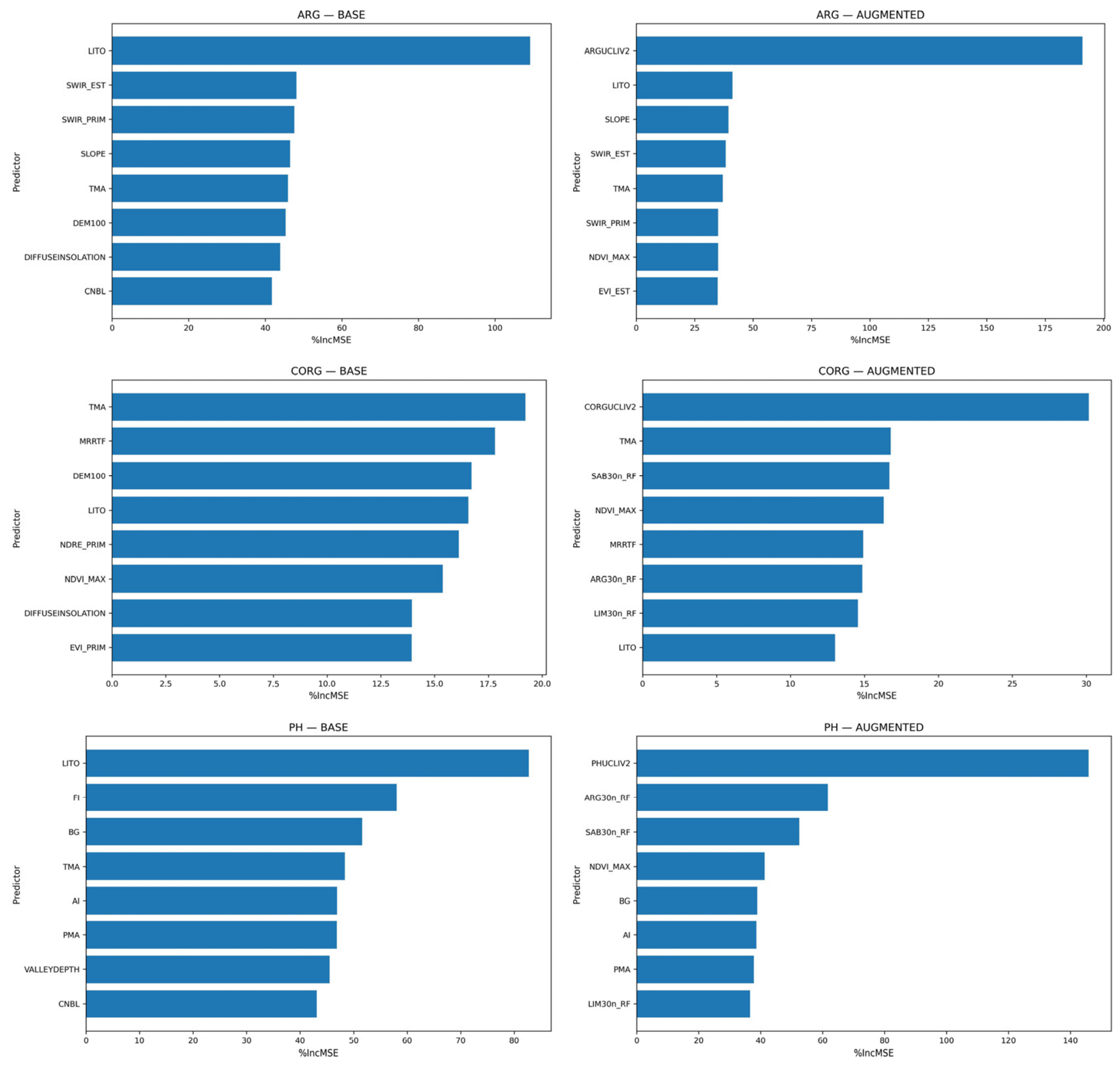
In the BASE configuration, importance was generally distributed across multiple environmental covariates. Lithology (LITO) consistently emerged as one of the most influential predictors for several soil properties (e.g., ARG, CACO3, PH), confirming the strong control exerted by parent material. Terrain attributes and remote sensing indices also contributed, indicating the combined influence of geomorphological and surface-related processes. However, the strength and structure of these relationships varied among variables: importance patterns were well defined for ARG, whereas they were weaker and more diffuse for CORG.
The AUGMENTED configuration substantially modified these patterns. Soil-derived predictors became dominant for several properties, particularly ARG, LIM, SAB, and PH, often concentrating a large proportion of the model explanatory power in a single variable. In these cases, the contribution of environmental covariates became secondary, indicating a strong reliance on pre-existing soil information.
This behavior was not uniform across all variables. For CSC and DA, importance remained distributed across multiple predictors, suggesting more complex controls. For CORG, the inclusion of soil-derived predictors led to only limited changes, and importance values remained relatively evenly distributed, indicating the absence of a dominant driver.
Overall, the results highlight that the effect of augmented predictors is strongly variable-dependent, with substantial improvements for structurally controlled properties such as ARG and pH, while more limited effects are observed for variables such as CORG, which are influenced by multiple interacting processes that are only partially represented by the available covariates (Figure 2).
Figure 2.
Variable importance (% increase in MSE) for three representative soil properties (ARG, CORG, and pH) under the BASE and AUGMENTED configurations. Only the eight most important covariates are shown for each soil property and configuration. In the BASE configuration, importance is distributed among multiple environmental covariates, with lithology and terrain attributes playing a key role. In the AUGMENTED configuration, soil-derived predictors dominate for structurally controlled variables (e.g., ARG and pH), whereas a more distributed importance pattern is retained for variables with more complex controls (e.g., CORG). Full names and descriptions of all covariates are reported in Appendix A, Table A1.
3.5. Spatial Predictions
Spatial predictions of selected soil properties (0–30 cm) were generated using Random Forest (RF), Quantile Regression Forest (QRF), and RF-REGIME5 models across the study area. Representative maps for clay content (ARG), soil organic carbon (CORG), and pH are presented to illustrate the spatial variability captured by the different modelling approaches.
The three models produced broadly consistent patterns at regional scale, indicating a robust representation of the main environmental gradients controlling soil variability. Differences among models were mainly observed at local scale, particularly in transitional areas and in zones characterized by higher environmental complexity.
Clay content (ARG) exhibits a well-defined and structured pattern across all models, with a high degree of agreement in the identification of major geomorphological domains. Mountainous areas are consistently associated with lower values, whereas plains and valley bottoms show higher clay contents, particularly in areas such as the Arno Valley. Despite this overall coherence, differences emerge in the representation of intermediate and high values. RF and QRF produce very similar outputs, characterized by sharper contrasts and more continuous high-value areas, whereas RF-REGIME5 shows a smoother pattern with reduced extremes and a tendency toward intermediate classes, especially in transitional zones (Figure 3).
Figure 3.
Spatial distribution of clay content (ARG, 0–30 cm) predicted by (a) Random Forest (RF), (b) Quantile Regression Forest (QRF), and (c) RF-REGIME5 models. All approaches reproduce consistent large-scale patterns, with lower values in mountainous areas and higher contents in plains and alluvial systems. Differences among models mainly concern the representation of local variability and the extent of extreme values, with RF and QRF showing sharper spatial contrasts and RF-REGIME5 producing a smoother and more generalized patterns.
To further illustrate these differences, relative difference maps comparing QRF and RF-REGIME5 predictions against RF are provided in Appendix A (Figure A3).
An additional pixel-wise assessment of the independently predicted particle-size fractions, prior to compositional closure, was performed for all three modelling approaches under both predictor configurations. The mean sums of ARG, LIM, and SAB ranged from 97.71% to 100.77%, with mean absolute deviations from 100% ranging from 2.22 to 3.61 percentage points. The 95th percentiles of absolute deviations ranged from 5.81 to 7.95 percentage points. Depending on the model and predictor configuration, between 8.15% and 21.82% of valid pixels showed deviations exceeding 5 percentage points, whereas deviations exceeding 10 percentage points occurred in fewer than 3% of valid pixels. QRF generally exhibited larger compositional deviations than RF and RF-REGIME5. These results indicate that the independently predicted fractions were close to compositional closure on average, although appreciable deviations occurred at individual pixels.
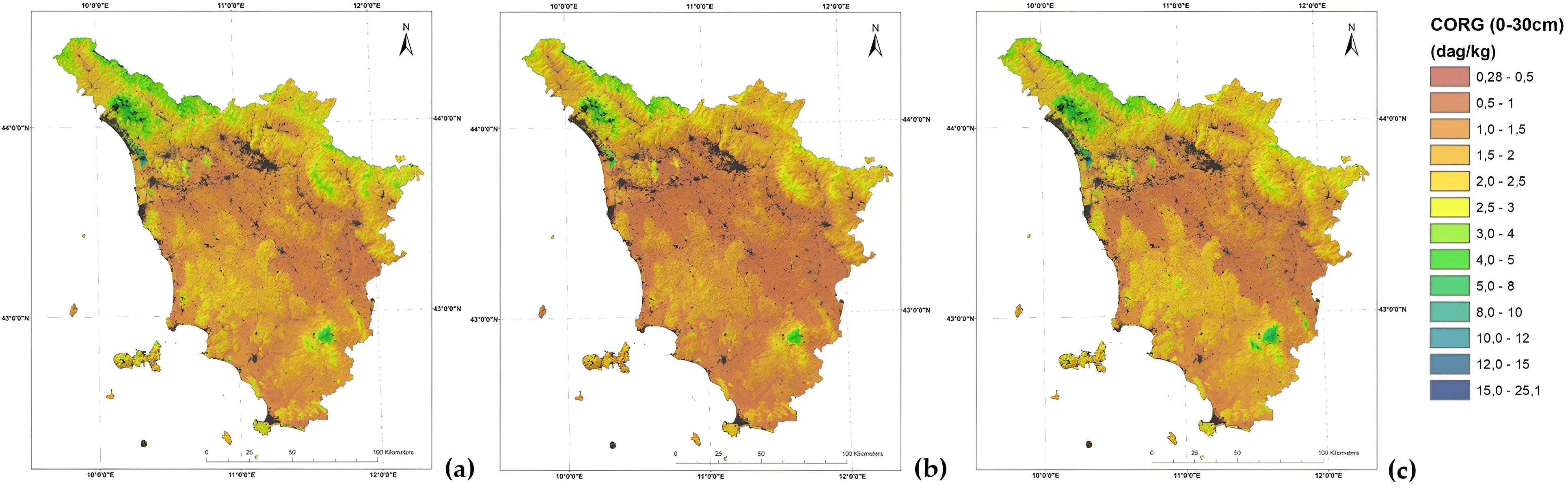
Soil organic carbon (CORG) displays a diffuse spatial distribution, with low to moderate values prevailing across most of the study area and higher concentrations confined to relatively limited and well-defined zones, such as the volcanic environments of Mount Amiata and the mountainous areas of the Apuan Alps. All models consistently identify these high-CORG areas, although their extent and intensity vary. RF and QRF highlight more distinct and spatially detailed hotspots, whereas RF-REGIME5 provides a more generalized representation, with smoother transitions and a reduced expression of extreme values (Figure 4).
Figure 4.
Spatial distribution of soil organic carbon (CORG, 0–30 cm) predicted by (a) Random Forest (RF), (b) Quantile Regression Forest (QRF), and (c) RF-REGIME5 models. All models show a broadly consistent pattern characterized by widespread low to moderate values and localized high-CORG areas. Differences among modelling approaches mainly concern the extent and intensity of these zones, with RF and QRF highlighting more distinct and spatially detailed hotspots, while RF-REGIME5 provides a smoother and more generalized representation.
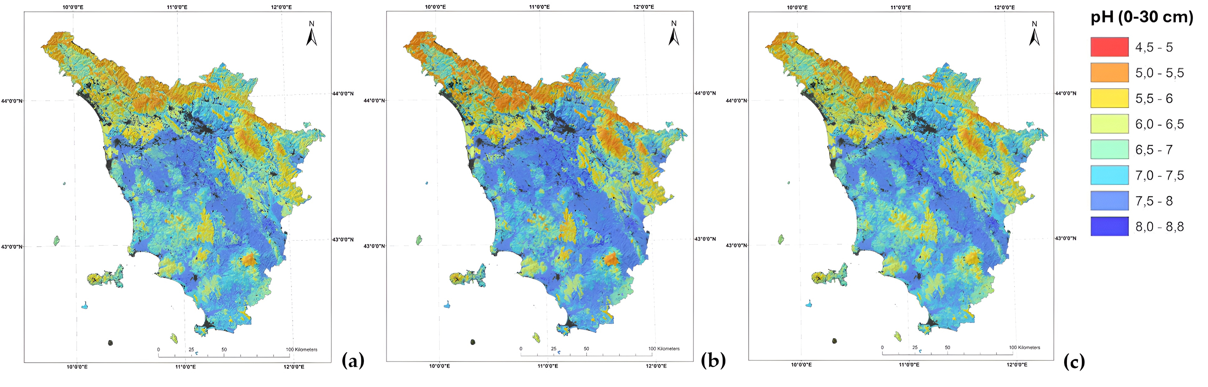
Soil pH shows the most spatially coherent pattern among the considered variables, with a clear large-scale organization and relatively smooth gradients. Acidic conditions dominate mountainous areas, such as the Mount Amiata and the Apennine higher ridge, while neutral to alkaline values prevail in lowland and alluvial systems such as the Lower Arno Valley. The three models are highly consistent in reproducing this pattern, with only minor differences at local scale. RF and QRF capture slightly finer spatial detail, whereas RF-REGIME5 produces a more smoothed representation (Figure 5).
Figure 5.
Spatial distribution of soil pH (0–30 cm) predicted by (a) Random Forest (RF), (b) Quantile Regression Forest (QRF), and (c) RF-REGIME5 models. All models show a highly consistent spatial pattern, with acidic conditions prevailing in mountainous areas and neutral to alkaline values in lowland and alluvial systems. Differences among modelling approaches are limited and mainly related to local variability, with RF and QRF capturing slightly finer spatial detail and RF-REGIME5 producing a smoother pattern.
The comparison indicates that model choice has a limited influence on the identification of large-scale spatial patterns while mainly affecting the representation of local variability and extreme values. These differences form the basis for interpreting model reliability, which is further examined through the analysis of prediction uncertainty.
The point-to-pixel comparison confirmed the consistency of the spatial prediction workflow, showing that differences between observed and predicted values reflect model performance rather than artefacts introduced during spatial processing, thereby supporting the reliability of the spatial outputs.
3.6. Prediction Uncertainty
For RF, prediction dispersion was quantified as the standard deviation of predictions across resampled model realizations, as described in Section 2.6. Due to the use of variable-specific quantile-based classification, the comparison focuses on relative spatial patterns rather than absolute uncertainty values. The spatial distribution of uncertainty varied markedly among soil properties (Figure 6). For clay content (ARG), uncertainty was widespread and spatially heterogeneous, with numerous areas of intermediate to high values across the region. For soil organic carbon (CORG), uncertainty was generally low over large portions of the study area but with localized hotspots corresponding to specific environmental settings. In contrast, soil pH showed a more continuous and homogeneous distribution of uncertainty, with fewer sharply defined peaks.
Figure 6.
Spatial distribution of prediction uncertainty (standard deviation) for (a) clay content (ARG), (b) soil organic carbon (CORG), and (c) soil pH (0–30 cm), derived from Random Forest models. Uncertainty is expressed as the standard deviation of predictions across resampled RF model realizations, reflecting variability associated with model recalibration. Due to the strongly skewed distribution of uncertainty values, maps are displayed using a quantile-based classification (nine classes) to enhance the visualization of spatial patterns and highlight areas of relatively higher uncertainty. Classes are defined independently for each variable and are therefore not directly comparable in absolute terms.
An exploratory analysis of relative prediction dispersion for CORG, using the RF model under the AUGMENTED configuration and expressing dispersion as the coefficient of variation (CV = SD/predicted value × 100), showed that normalization substantially reduced the association between predicted values and dispersion (Spearman’s ρ decreasing from 0.733 for SD to 0.279 for CV). This indicates that the spatial pattern of absolute SD is partly influenced by the magnitude of predicted CORG values.
These patterns indicate that model stability is strongly property-dependent and reflects the complexity of the underlying soil–environment relationships. For ARG and CORG, higher uncertainty values tend to co-occur with areas of higher predicted values, suggesting greater variability and reduced representation of extreme conditions within the training dataset.
Although uncertainty maps are shown for the Random Forest model, similar spatial patterns were observed for the RF-REGIME5 approach, which is based on a comparable standard deviation metric. In contrast, Quantile Regression Forest (QRF) expresses uncertainty through the spread of predicted quantiles, making direct comparison with standard deviation-based measures inappropriate. Nevertheless, consistent spatial agreement in the location of higher and lower uncertainty areas can be observed across models, although QRF displays a more fragmented and locally variable pattern compared to the smoother distributions produced by RF and RF-REGIME5 (Figure 7).
Figure 7.
Spatial distribution of prediction dispersion for soil organic carbon (CORG) derived from three models: (a) Random Forest (RF), represented by the resampling-based prediction standard deviation; (b) Quantile Regression Forest (QRF), represented by the quantile-based predictive standard deviation, approximated as (Q95 − Q05)/3.29; and (c) RF-REGIME5, represented by the regime-specific resampling-based prediction standard deviation.
The maps highlight different spatial patterns of predictive dispersion across the study area, with RF and RF-REGIME5 showing relatively low prediction variability in several areas, while QRF exhibits more localized areas of high predictive dispersion. These differences reflect the distinct uncertainty estimation procedures adopted by the three modelling approaches. Because the reported measures capture different components of predictive uncertainty, the maps are intended primarily for qualitative comparison of relative spatial patterns and should not be interpreted as directly comparable indicators of absolute uncertainty, model accuracy, or reliability.
The empirical coverage of nominal 90% QRF prediction intervals exceeded 90% for all ten properties, ranging from 92.7% to 97.9% under BASE and from 93.3% to 97.1% under AUGMENTED. Mean interval widths were lower under AUGMENTED for every property (reductions of 1.2–15.3%), decreasing, for example, from 35.32 to 31.02 dag/kg for ARG and from 2.42 to 2.26 dag/kg for CORG. Tail exceedances were sometimes asymmetric. For CACO3, the proportions falling below Q05 and above Q95 were 0.10% and 3.49% under BASE, compared with 0.60% and 2.59% under AUGMENTED. The corresponding QCP05 values (21.0% and 21.5%) reflected numerous observations exactly coinciding with Q05, predominantly at zero.
4. Discussion
The comparison of modelling approaches highlights marked differences in predictive performance among soil properties, with the relative influence of predictor information and modelling strategy varying across properties.
Variables such as pH, characterized by strong links with lithology and large-scale environmental gradients, show high spatial coherence and predictability, consistent with previous findings in digital soil mapping [6,25]. In contrast, soil organic carbon (CORG) exhibits lower predictive performance and a more diffuse spatial structure, reflecting the influence of multiple interacting and partially unresolved drivers, including land use, land management, and biological processes, which are often difficult to capture through environmental covariates alone [26]. Although remotely sensed vegetation indices were included among the predictors, explicit land-use variables were not retained in the final models. The available land-use datasets, originally mapped at 1:10,000 scale using third-level CORINE Land Cover categories, presented potential limitations associated with their rasterization to the 100 m modelling grid, including loss of spatial detail and mixed-pixel effects. Furthermore, the CORINE classification does not provide explicit information on land-management practices, which are particularly relevant to soil organic carbon dynamics. Consequently, the absence of detailed land-use and management information remains a potential limitation in modelling local CORG variability.
Clay content (ARG) represents an intermediate case, where both lithological and geomorphological controls are effectively captured, as observed in clay-rich landscapes such as the Crete Senesi, Val d’Orcia and the lower Arno Valley, although local variability remains only partially explained. These patterns indicate that model performance in digital soil mapping largely reflects the degree to which soil-forming processes are structured and represented by the available covariates [6].
The spatial structure of the soil properties provides a quantitative basis for interpreting the validation results. Nugget-to-sill ratios of 0.39–0.68 indicate that approximately half of the variance of each soil property is spatially structured, with the remaining half attributable to short-range variation or analytical noise. The double-range structure observed for nine of the ten properties reflects the multi-scale nature of soil variation in Tuscany, with a short-range component (3–14 km) linked to local soil-forming processes and a long-range component (17–40 km) linked to regional climatic and geological gradients. This structure has direct implications for the interpretation of the performance metrics reported in Table 5, Table 6 and Table 7. Because the long-range component operates well beyond the observations spacing, it does not contribute to the bias introduced by random split validation. The short-range component does extend across a few nearest neighbors, but it accounts for only a limited fraction of the total variance. The absolute performance values should therefore be interpreted as upper bounds on true out-of-sample performance, while the relative comparison between RF, QRF, and RF-REGIME5—the central contribution of this study—is minimally affected because all models were evaluated on the same split.
This property-specific picture also reinforces the interpretation of the AUGMENTED configuration developed earlier. Properties with the strongest short-range structure and the highest nugget-to-sill ratios (skeleton, carbonates) are those for which the AUGMENTED configuration provides the smallest gains, because map-unit attributes operate at a coarser spatial resolution than the short-range processes controlling these properties. Conversely, properties with a well-defined and spatially continuous structure (clay, pH, CSC) benefit most from the integration of map-unit knowledge, which operates at the same spatial scales as the dominant soil-forming processes.
An additional limitation arises from the temporal heterogeneity of the regional soil database, which combines observations collected over several decades. Although analytical harmonization was applied where necessary, no temporal standardization of soil property values was performed. This limitation is particularly relevant for soil organic carbon, whose temporal evolution is strongly influenced by land management practices that are not systematically documented in regional soil databases. Consequently, retrospective adjustment of historical carbon measurements to a common reference year was considered insufficiently reliable. The temporal sensitivity of other properties varies: soil pH may remain relatively stable under unchanged environmental and management conditions, whereas bulk density in cultivated topsoil can exhibit substantial short-term variations associated with tillage and compaction.
Furthermore, combining historical soil observations with recent Sentinel-2 covariates may weaken the inferred relationships between soil properties and environmental predictors, particularly for CORG in areas where land cover or agricultural management has changed since soil sampling.
Together, these factors introduce an additional source of uncertainty that cannot be explicitly quantified with the available information. Therefore, the resulting maps should be interpreted as spatial representations integrating observations from different periods, rather than as temporally standardized estimates of present-day soil conditions.
Within this context, the limited improvement observed for the regime-based approach (RF-REGIME5) can be interpreted as a consequence of the trade-off between environmental homogeneity and sample size. While spatial stratification reduces internal variability, it simultaneously restricts the number of observations available for model calibration, thereby constraining the ability to learn complex relationships. Similar limitations of stratified or local modelling approaches have been reported in heterogeneous landscapes, where gains from reduced variance are offset by reduced data support [8,27]. This behavior is consistent with previous studies emphasizing the role of spatial transferability and domain-specific modelling in digital soil mapping [8,24,28] and extends these approaches by linking model performance across domains to the definition of modelling units.
Moreover, the persistence of substantial variability within regimes suggests that soil–environment relationships vary more continuously than discretely, limiting the effectiveness of hard regionalization schemes. These results indicate that, at regional scale, global models can provide comparable or more stable performance when data density is insufficient to support local model calibration.
Although the sampling locations provide broad geographical coverage of Tuscany, this does not necessarily ensure complete representation of the environmental predictor space. Since no formal Area of Applicability (AOA) analysis was performed, areas with environmental conditions poorly represented in the training data could not be identified [29,30,31]. Consequently, predictions in these areas may be less reliable than suggested by the overall test-set performance metrics, and their uncertainty may not be adequately characterized. This also limits our ability to identify where additional validation or soil sampling would be the most needed.
Consistently across all modelling approaches, the inclusion of soil-derived predictors (AUGMENTED configuration) resulted in improved predictive performance, confirming that model accuracy is primarily data-driven. The magnitude of this improvement was largely independent of the modelling strategy, highlighting the dominant role of predictor quality over algorithm choice, in agreement with previous studies emphasizing the importance of covariate selection in DSM [8,24]. However, the effect was strongly variable-dependent, and the structure of this variability is itself informative. The largest gains were observed for properties with strong subsoil control—clay, silt, sand, pH, and cation exchange capacity—whereas the weakest gains were observed for soil organic carbon, which is predominantly controlled by surface processes (land use, litter input, microbial activity) that are already partially captured by remote sensing and climatic covariates. This pattern is consistent with the interpretation that the map-unit predictors encode profile-scale pedological knowledge—particularly subsoil properties, drainage conditions, and parent material weathering—that surface-derived covariates cannot represent. Soil map units are delineated by integrating the full soil profile concept, including horizonation, depth, and drainage, whereas environmental covariates describe only the uppermost boundary conditions. For topsoil properties whose spatial distribution is partly inherited from subsoil processes such as clay translocation, carbonate dynamics, and weathering fronts, this information is otherwise inaccessible within a purely environmental covariate framework. The variable-dependent pattern of improvement therefore provides direct evidence that the AUGMENTED configuration does not merely add correlated numerical values but integrates two complementary information sources: continuous environmental covariates describing the surface boundary conditions, and discrete pedological knowledge describing the soil system as a whole. In this sense, the AUGMENTED configuration is not simply a data-augmentation exercise but an integration of two complementary representations of the soil-landscape. This interpretation also helps to explain why the improvement for CORG remained limited. Soil organic carbon is a dynamic, surface-driven property influenced by land management, litter input, and biological processes that operate at timescales and spatial scales not represented by the legacy map units, which were compiled primarily to describe relatively stable morphological and textural properties. The highly skewed distribution of CORG values, characterized by a large proportion of low to moderate values and a limited number of extreme observations reaching substantially higher concentrations, further reduces the ability of the models to adequately represent the full range of variability and may lead to reduced stability and increased uncertainty in specific environmental contexts.
The weighted sampling procedure also influenced the distribution of CORG observations between training and test datasets. Although designed to increase the representation of extreme values during model calibration, it resulted in a lower variability in the test dataset (SD = 0.89) than in the training dataset (SD = 1.56). An examination of the observed CORG values showed that both tails were represented in the test dataset, but only 16 of the 232 observations below the overall 5th percentile and 18 of the 232 observations above the overall 95th percentile were included. Moreover, only two observations above the overall 99th percentile were retained in the test dataset. Consequently, the reported test metrics mainly reflect predictive performance within the central portion of the observed distribution and provide a less robust assessment of model performance for extreme CORG values. The dataset included eight profiles classified as Histosols or their taxonomic equivalents, representing approximately 0.2% of the total observations. Their specific influence on CORG prediction accuracy was not quantified.
These findings suggest that environments associated with extreme CORG values, such as organic-rich soils (e.g., in the surroundings of Lake Massaciuccoli) or specific pedological settings, may not be optimally represented within a single regional modelling framework. In this perspective, the adoption of targeted modelling strategies—such as the separate treatment of these environments or their exclusion from global calibration—could improve both model performance and interpretability. This highlights that model performance is constrained by the representativeness of the available data, particularly in complex and weakly structured systems, and that the value of legacy soil information is greatest where the target property has a strong, conceptually well-defined relationship with the pedolandscape.
The use of soil-derived predictors in the AUGMENTED configuration nonetheless requires careful interpretation, as it may introduce partial redundancy with the target variables. Rather than representing a limitation, this aspect was explicitly addressed in the modelling design by distinguishing between BASE and AUGMENTED configurations, allowing for separation of the contribution of environmental covariates from that of prior soil knowledge.
In this context, the observed improvements in the AUGMENTED configuration should not be interpreted solely as enhanced predictive skill but also as the effect of integrating pre-existing spatial information. This highlights the difference between purely data-driven modelling and hybrid approaches that incorporate legacy soil information.
The direct comparison with the legacy soil map-unit estimates further qualifies the benefits of the AUGMENTED configuration. While substantial improvements were observed for several soil properties, the additional predictive gain over existing map-unit information was marginal for ARG and LIM. For these properties, the legacy estimates themselves already provided relatively high predictive performance. Moreover, the improvements achieved by AUGMENTED reflect the combined contribution of its predictor set and cannot be attributed exclusively to individual legacy layers.
While the latter can substantially improve prediction accuracy, particularly for structurally controlled properties, they may also reduce the independence of predictions, especially when soil-derived predictors are closely related to the target variables. Their use should therefore be carefully evaluated depending on the intended application, particularly in contexts where independent prediction is required.
For soil monitoring applications, the use of pre-existing soil information requires additional consideration. The regional soil database integrates observations collected over several decades, with older surveys predominating, but more recent observations also represented. Consequently, the soil map-unit attributes should not be interpreted as representing conditions at a single historical reference date. Nevertheless, their inclusion as predictors may reinforce established spatial patterns and potentially reduce sensitivity to temporal changes not captured by the available covariates, particularly for dynamic properties such as soil organic carbon. Assessing the suitability of the AUGMENTED configuration for detecting soil changes over time would therefore require temporally referenced validation data.
These considerations provide a framework for interpreting the observed patterns of prediction uncertainty. Although RF, RF-REGIME5, and QRF show general agreement in the spatial location of higher and lower uncertainty areas, they differ in how uncertainty is expressed. RF and RF-REGIME5 produce relatively smooth and spatially coherent patterns, reflecting ensemble stability, whereas QRF exhibits a more fragmented structure, capturing local variability and distributional features such as skewness and extreme values. This difference is consistent with the theoretical properties of quantile regression forests, which estimate the full conditional distribution rather than a single central tendency [9]. Importantly, this behavior does not indicate lower reliability of QRF but rather a higher sensitivity to fine-scale variability.
The uncertainty maps produced by RF, RF-REGIME5, and QRF should be interpreted with caution, as they represent different components of predictive uncertainty. While RF and RF-REGIME5 quantify variability across resampled model predictions, QRF provides a quantile-based approximation of the dispersion of the conditional predictive distribution. Consequently, these measures are not directly comparable and should not be used to assess the relative predictive accuracy or reliability of the three modelling approaches.
The broadly consistent spatial patterns of prediction dispersion across models suggest that environmental heterogeneity and the available predictor information may influence their spatial distribution, while model-specific uncertainty measures affect their expression. This interpretation is consistent with recent DSM research showing that local prediction uncertainty depends on the contributions of individual environmental covariates [32]. The stronger association between high predicted values and higher absolute prediction dispersion, particularly for ARG and CORG, should also be interpreted in light of the limited overall frequency of extreme observations and the dependence of absolute dispersion on the magnitude of predicted values.
Although QRF interval coverage consistently exceeded the nominal 90% level, this alone does not establish optimal calibration, as high coverage may also result from excessively wide intervals. The reduced mean interval widths under AUGMENTED indicate improved average sharpness while maintaining coverage above the nominal level. Differences between lower- and upper-tail exceedance rates suggest asymmetric interval behaviour for some properties, although quantile coverage probabilities require caution when observations coincide with predicted quantile boundaries, particularly for zero-inflated variables. These findings remain subject to the limitations of the adopted random hold-out validation and do not establish spatially independent uncertainty calibration. A comparable empirical calibration of the resampling-based dispersion measures obtained from RF and RF-REGIME5 was not performed.
A more rigorous comparison of predictive uncertainty across the three modelling approaches would require constructing prediction intervals at a common nominal coverage level, for example 90%, and evaluating them on the same independent test observations. For RF and RF-REGIME5, such intervals could be obtained through residual-based calibration, potentially using conformal prediction methods, to account for predictive variability not captured by the resampling-based standard deviations. These could then be compared with the QRF quantile-based intervals in terms of empirical coverage, interval width, and interval score [33,34]. This approach would provide a common basis for assessing probabilistic predictive performance, although its implementation and spatially independent validation were beyond the scope of the present study.
Taken together, these results suggest that Random Forest represents a practical approach for regional-scale applications, providing competitive predictive performance across different soil properties, as widely reported in environmental modelling studies [7,8]. However, the choice of modelling strategy should be guided by the specific objectives of the analysis. While RF is well suited for generating reliable spatial predictions, QRF offers additional insight into the distribution of possible outcomes and is particularly valuable when uncertainty characterization is a primary goal. This is especially relevant for variables with skewed distributions or pronounced extreme values, where the ability to estimate conditional quantiles provides a more complete representation of the response behavior and supports more informed interpretation and decision-making.
More broadly, within the RF-based approaches investigated here, the AUGMENTED configuration consistently improved predictive performance across all soil properties, although the relative influence of predictor enrichment and modelling strategy varied among properties. In particular, for CORG and PROF, differences in NSE among modelling approaches exceeded the improvements associated with the AUGMENTED configuration. A similar pattern was observed for CACO3, particularly under the BASE configuration.
Improving the quality and representativeness of covariates, together with increasing the density and coverage of soil observations, remains the most effective pathway to enhance predictive performance and reduce uncertainty, particularly in heterogeneous environments.
In addition, recent developments in machine learning suggest that alternative algorithms such as gradient boosting methods (XGBoost; [35]) may offer further improvements in predictive performance for complex soil properties, particularly soil organic carbon. Preliminary results presented in the conference proceedings of ASITA 2024 [36] have highlighted the potential of these approaches when integrated with advanced hyperparameter optimization frameworks. Ongoing work in this direction aims to systematically compare these methods with Random Forest-based approaches within the current modelling framework.
From an operational perspective, the results of this study are relevant to the implementation of the EU Soil Monitoring Law (Directive (EU) 2025/2360), which establishes a common framework for assessing soil health through standardized soil descriptors. Several properties mapped in this study are directly related to these requirements. In particular, soil organic carbon (CORG) and clay content (ARG) provide the spatial information needed to support the assessment of the SOC-to-clay ratio, a descriptor used to evaluate soil organic carbon status in mineral soils. Soil pH is directly relevant to the assessment of acidification, while bulk density (DA) and particle-size distribution provide information relevant to soil compaction. Additional properties, including soil depth, coarse fragments, cation exchange capacity, and calcium carbonate content, contribute complementary information for characterizing soil functions and potential degradation processes.
Although clay, silt, and sand were modelled independently, their predicted values can be made compositionally consistent through proportional closure, as applied to the RF-derived texture covariates in the AUGMENTED configuration. Log-ratio transformations provide an alternative approach to compositional prediction [37,38,39]. However, previous comparisons indicate that improvements in predictive accuracy are not systematic and may depend on the modelling approach and evaluation criteria [38,39]. The accuracy of derived indicators, such as the SOC-to-clay ratio, was not independently evaluated in this study. Therefore, for applications requiring compositionally consistent texture (e.g., SOC-to-clay ratio within the EU Soil Monitoring Law), the three fractions should be closed proportionally before use.
Within the limitations already discussed, the resulting maps provide a spatially explicit knowledge base to support the implementation of regional soil monitoring programmes. In particular, the combined analysis of mapped soil properties, pedoenvironmental variability, and spatial patterns of prediction uncertainty can contribute to the identification of representative monitoring areas and the selection of sampling locations. These spatial products can support the stratification of the territory into different soil and environmental conditions while highlighting areas characterized by greater variability or uncertainty where additional observations may be particularly valuable. In this perspective, digital soil mapping can contribute not only to the preliminary assessment of soil conditions but also to the planning and progressive optimization of monitoring networks, supporting the establishment of an effective and spatially representative soil monitoring framework in accordance with the objectives of the EU Soil Monitoring Law.
5. Conclusions
This study compared three Random Forest-based modelling strategies for predicting topsoil properties across Tuscany. The results demonstrate that the inclusion of legacy soil-derived predictors (AUGMENTED configuration) consistently improved predictive accuracy across all models, while the choice between RF, QRF, and regime-based approaches had only marginal effects on performance. These findings lead to the following conclusions and practical recommendations.
For regional-scale DSM in heterogeneous landscapes, our results highlighted that the choice of input covariates has a greater impact on predictive accuracy than the choice between RF, QRF, or regime-based strategies. Therefore, the AUGMENTED configuration is recommended whenever prior spatial soil information is available and independent prediction is not a strict requirement. In this context, the value of legacy soil information should be understood not only in terms of statistical correlation with the target variables but also in terms of the profile-scale pedological knowledge it encodes. Soil map units integrate subsoil properties, drainage conditions, and parent material weathering that surface-derived covariates cannot represent, and the variable-dependent pattern of improvement observed in this study—strongest for subsoil-controlled properties such as clay, pH, and CEC—supports this interpretation. Legacy soil maps should therefore be regarded as a conceptual complement to environmental covariates, rather than as a redundant predictor set.
Based on the study’s objectives and typical DSM applications, standard Random Forest (RF) represents a practical choice for general-purpose spatial prediction, providing competitive predictive performance across most soil properties. However, QRF achieved better predictive accuracy for CORG and offers the additional advantage of estimating conditional prediction intervals, making it particularly useful when uncertainty characterization is a primary objective.
Resorting to a regime-based approach (RF-REGIME5) is recommended only when (a) sample size within each stratum is sufficiently large, and (b) there is strong prior evidence that soil–environment relationships differ substantially across domains. For the Tuscany dataset, the global models were generally preferable.
For Tuscany, hard regionalization into five pedo-landscape domains did not improve predictive performance over a single global model. This suggests that soil–environment relationships vary more continuously than discretely at this scale. Future work should explore soft regionalization or spatially varying coefficient models instead of discrete strata. Additionally, standard regional models failed to represent localized extreme values, particularly for organic-rich soils. For variables with highly skewed distributions and for specific environmental niches, alternative strategies should be considered, such as stratified sampling to increase representation of tail values, separate modelling of organic and mineral soils where sufficient observations are available, or targeted local models for specific pedological hotspots.
The resulting maps (e.g., for CORG, ARG, and pH) can support regional-scale assessments of soil properties relevant to soil degradation and ecosystem services. However, their use should account for property-specific predictive limitations, particularly the moderate accuracy for CORG (R2 ≈ 0.3), and the spatial variability in prediction uncertainty. These maps should therefore be considered supporting information rather than stand-alone evidence for site-specific assessments or management decisions.
Beyond their predictive value, the resulting soil property and uncertainty maps provide a spatially explicit knowledge base to support the implementation of the EU Soil Monitoring Law, particularly by informing territorial stratification and guiding the selection of representative sampling locations for future soil monitoring networks.
Increasing the density and spatial coverage of soil observations, particularly in underrepresented environments (e.g., organic-rich soils, mountainous areas), remains the most effective pathway to improving DSM predictions in Tuscany—more so than further algorithmic refinement. Future work should prioritize targeted sampling in the high-uncertainty zones identified in this study.
Author Contributions
Conceptualization, L.G., R.L. and F.U.; methodology, L.G., R.L. and F.U.; formal analysis, L.G., R.L. and F.U.; data curation, L.G., R.L. and F.U.; writing—original draft preparation, L.G., R.L. and F.U.; writing—review and editing, L.G., R.L. and F.U.; visualization, L.G., R.L. and F.U.; project administration, R.L. and F.U.; funding acquisition, F.U. All authors have read and agreed to the published version of the manuscript.
Funding
This research was funded by the SERENA project. SERENA (Soil Ecosystem seRvices and soil threats modElling aNd mApping) is an EJP SOIL internal project. EJP SOIL has received funding from the European Union’s Horizon 2020 research and innovation program: Grant agreement No. 862695.
Data Availability Statement
The Random Forest soil property maps presented in this study are publicly available for download at https://zenodo.org/records/14039386 (accessed on 10 September 2026). The comparative performance results of the RF, QRF, and RF-REGIME5 approaches are reported in the manuscript and its appendices. The underlying soil observations were derived from the Tuscany Region soil database and additional datasets kindly provided by the LaMMA Consortium.
Acknowledgments
The authors gratefully acknowledge the LaMMA Consortium (Laboratory for Monitoring and Environmental Modelling for Sustainable Development) for providing access to the Tuscan pedological and environmental datasets used in this study. The availability of these datasets was essential for the development and completion of the research. The authors wish to thank the three anonymous reviewers whose comments and suggestions contributed to improve the scientific rigor and the quality of the manuscript.
Conflicts of Interest
The authors declare no conflicts of interest.
Abbreviations
The following abbreviations are used in this manuscript:
| AI | Aridity index |
| AOA | Area of Applicability |
| ARG | Clay content (0–30 cm; dag/kg) |
| ARG30n_RF | Clay content (0–30 cm; dag/kg) derived from DSM |
| ARGUCLIV2 | Clay content (0–30 cm; dag/kg) derived from existing soil maps |
| BG | Bagnouls–Gaussen Index |
| BSI_EST | Summer Bare soil index |
| BSI_PRIM | Spring Bare soil index |
| CACO3 | Total carbonate content (0–30 cm; dag/kg) |
| CI | Convergence Index |
| CNBL | Channel Network Base Level |
| CORG | Organic carbon content (0–30 cm; dag/kg) |
| CORG30_RF | Organic carbon content (0–30 cm; dag/kg) derived from DSM |
| CORGUCLIV2 | Organic carbon content (0–30 cm; dag/kg) derived from existing soil maps |
| CSC | Cation Exchange Capacity (0–30 cm; meq/100 g) |
| CSCUCLIV2 | Cation Exchange Capacity (0–30 cm; meq/100 g) derived from existing soil maps |
| C-stock | Soil organic carbon stock (0–30 cm; t/ha) |
| DA | Bulk Density (0–30 cm; g/cm3) |
| DEM | Digital Elevation Model |
| DEM100 | 100 m Digital Elevation Model resampled from the regional 10 m DEM |
| DIFFUSEINSOLATION | Diffuse insolation |
| DIRECTINSOLATION | Direct insolation |
| DSM | Digital Soil Mapping |
| EJP SOIL | European Joint Programme Soil |
| EU | European Union |
| EVI_EST | Summer Enhanced Vegetation Index |
| EVI_PRIM | Spring Enhanced Vegetation Index |
| FI | Fournier modified Index |
| GHG | Greenhouse gas |
| IPCC | Intergovernmental Panel on Climate Change |
| IUSS | International Union of Soil Sciences |
| LaMMA | Laboratory for Environmental Monitoring and Modeling for Sustainable Development |
| LIM | Silt content (0–30 cm; dag/kg) |
| LIM30n_RF | Silt content (0–30 cm; dag/kg) derived from DSM |
| LIMUCLIV2 | Silt content (0–30 cm; dag/kg) derived from existing soil maps |
| LITO | Lithology map |
| LS | Slope Length |
| MBI | Mass Balance Index |
| MiPAAF | Ministero dell’Agricoltura, della Sovranità alimentare e delle Foreste |
| MRRTF | Multi-resolution Ridge Top Flatness |
| MRVBF | Multi-resolution Valley Bottom Flatness |
| MSI_EST | Multi-year mean summer MSI (Moisture Stress Index). |
| MSI_PRIM | Multi-year mean spring MSI (Moisture Stress Index). |
| mtry | number of variables randomly sampled at each split |
| NDMI_EST | Multi-year mean summer NDMI (Normalized Difference Moisture Index). |
| NDMI_PRIM | Multi-year mean spring NDMI (Normalized Difference Moisture Index). |
| NDRE_EST | Multi-year mean summer NDRE (Normalized Difference Red Edge). |
| NDRE_PRIM | Multi-year mean spring NDRE (Normalized Difference Red Edge). |
| NDVI_EST | Multi-year mean summer NDVI. |
| NDVI_MAX | Multi-year mean annual maximum NDVI. |
| NDVI_PRIM | Multi-year mean spring NDVI. |
| NSE | Nash–Sutcliffe efficiency |
| pH | pH in water (0–30 cm) |
| PHUCLIV2 | pH in water (0–30 cm) derived from existing soil maps |
| PLANCURVATURE | Plan curvature |
| PMA | Mean annual precipitation (mm) |
| PROF | Soil depth (cm) |
| PROFILECURVATURE | Profile curvature |
| PROFUCLIV2 | Soil depth (cm) derived from existing soil maps |
| QCP | Quantile Coverage Probability |
| QRF | Quantile Random Forest |
| RELATIVESLOPEPOSITION | Relative slope position |
| R2 | Squared Pearson correlation coefficient between observed and predicted values |
| RF | Random Forest |
| RF-REGIME5 | Random Forest Regime-based model |
| SAB | Sand content (0–30 cm; dag/kg) |
| SAB30n_RF | Sand content (0–30 cm; dag/kg) derived from DSM |
| SABUCLIV2 | Sand content (0–30 cm; dag/kg) derived from existing soil maps |
| SAGA | System for Automated Geoscientific Analyses |
| SERENA | Soil Ecosystem seRvices and soil threats modElling aNd mApping Project |
| SG | Geographical Systems |
| SIPT | Information Systems and Spatial Planning |
| SKEL | Rock fragment content (0–30 cm; vol/vol) |
| SKELUCLIV2 | Rock fragment content (0–30 cm; vol/vol) derived from existing soil maps |
| SLOPE | Terrain slope derived from the DEM |
| SP | Stream Power Index. |
| SP2 | Modified Stream Power Index. |
| SR | Soil region |
| SWIR_EST | Short-Wave Infrared value for the summer period (June-September 2022) |
| SWIR_PRIM | Short-Wave Infrared mean value in spring |
| TMA | Mean annual Temperature (°C) |
| TPI20 | Multiscale Topographic Position Index at 200 m scale |
| TPI5 | Multiscale Topographic Position Index at 50 m scale |
| TWI | Topographic Wetness Index |
| UCLIV2 | Level-2 soil mapping units (1:50,000 scale) |
| VALLEYDEPTH | Valley depth |
| VDCN | Vertical distance to channel network |
| WRB | World Reference Base |
Appendix A
Table A1.
List and description of environmental covariates.
Figure A1.
Spatial distribution of soil sampling locations used for clay content (ARG) modelling (n = 4500) across the seven Soil Regions of Tuscany. Red dots indicate sampling locations, while grey lines represent Soil Region boundaries. Soil Region codes identify the following pedoenvironmental domains: 78.2—Apennine mountains; 60.41—Apuan Alps; 64.4—inland alluvial and northern coastal plains; 60.4—mixed-lithology hilly and mountainous landscapes; 61.3—hills developed on Neogene sediments; 60.7—coastal plains and islands; 56.1—southern volcanic landscapes. Both training and test observations are included.
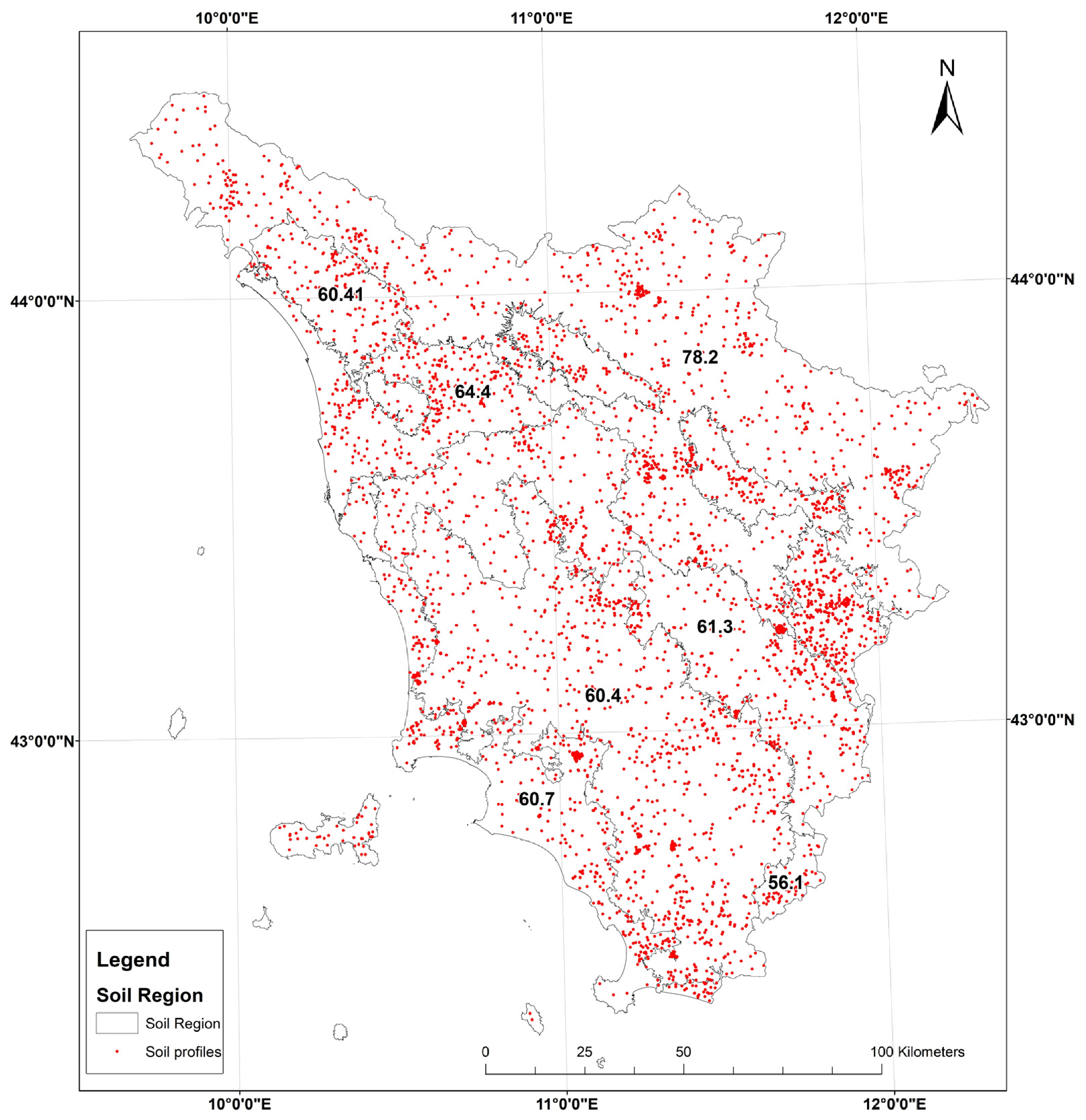
Figure A2.
Experimental (black dots) and modelled (red lines) semivariograms for soil properties: (a) sand content (%, 0–30 cm); (b) silt content (%, 0–30 cm); (c) clay content (%, 0–30 cm); (d) organic carbon (%, 0–30 cm); (e) pH (-, 0–30 cm); (f) Cation Exchange Capacity (meq/100 g, 0–30 cm); (g) Bulk density (Mg/m3, 0–30 cm); (h) Coarse fraction (%, 0–30 cm); (i) Soil depth (cm); (j) Total CaCO3 (%, 0–30 cm). The parameters of semivariograms models are reported in Table 3.
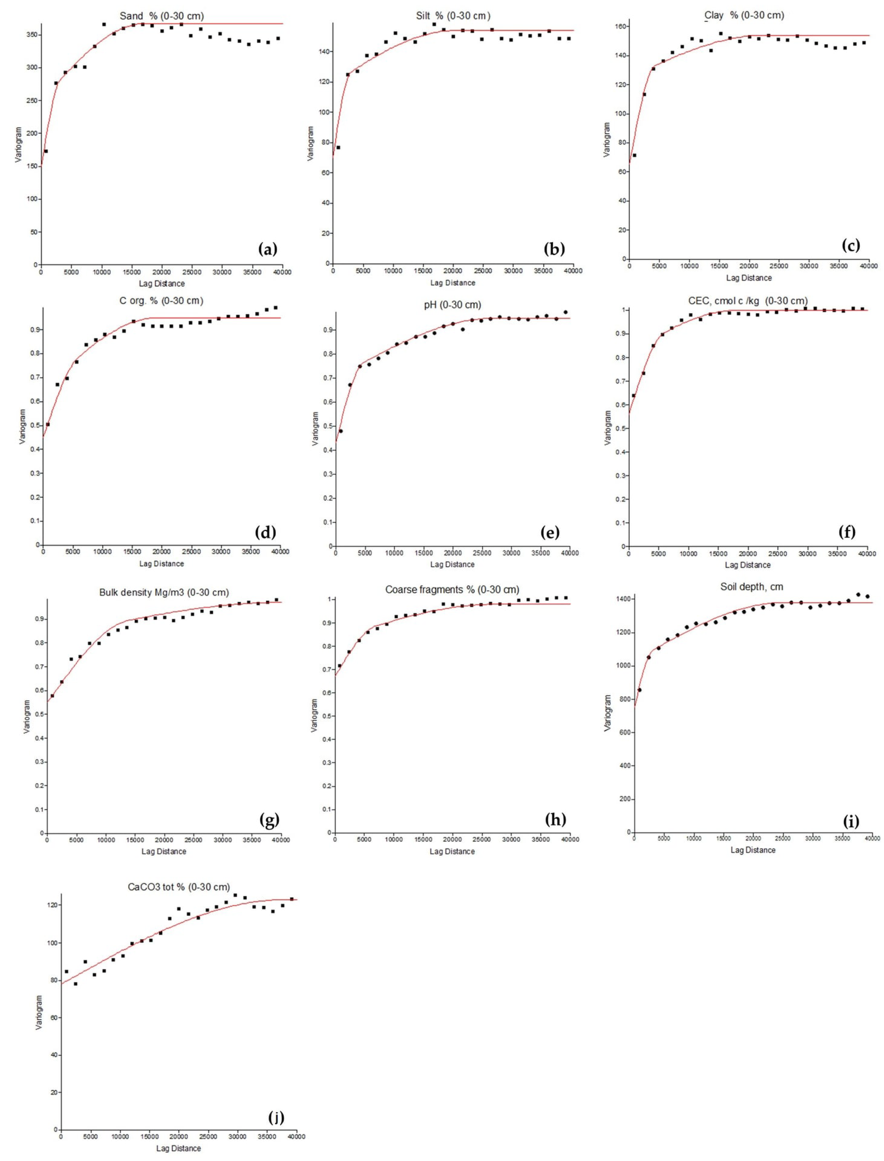
Figure A3.
Spatial distribution of relative differences (%) in clay content (ARG, 0–30 cm) predictions between (a) Quantile Random Forest (QRF) and Random Forest (RF), and (b) RF-REGIME5 and RF. Relative differences were calculated as [(Model − RF)/RF] × 100, using RF as the reference model. Positive and negative values indicate higher and lower predictions, respectively, compared with RF. Both maps use the same five-class classification scheme to facilitate comparison.
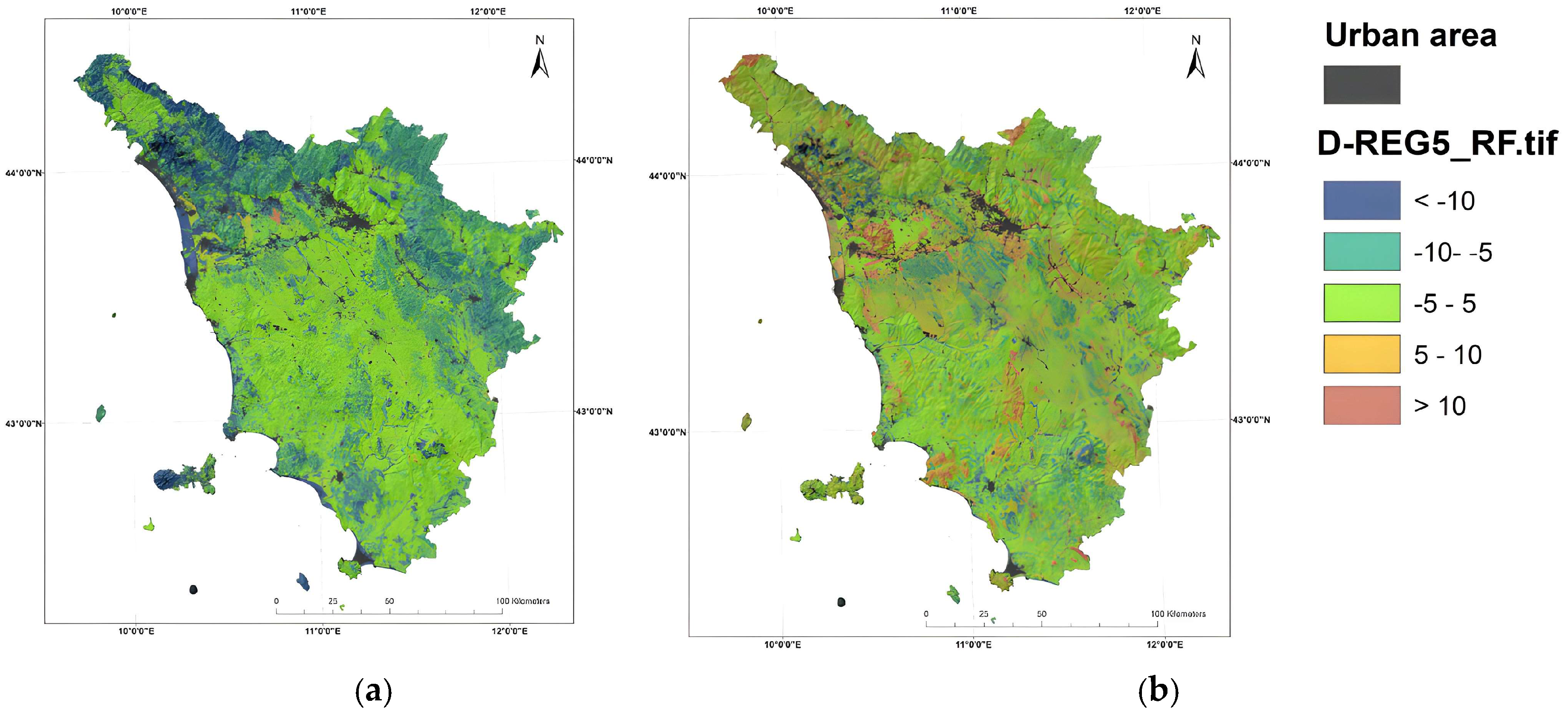
Table A2.
Test-set performance of pre-existing soil map-unit estimates (UCLIV2) and global Random Forest predictions under the BASE and AUGMENTED configurations for nine soil properties.
References
- Buttafuoco, G.; Montagne, D.; Hessel, R.; Asins-Velis, S.; Assennato, F.; Lemercier, B.; Coblinski, J.; Cockx, K.; Congedo, L.; Cousin, I.; et al. Deliverable D2.3.2 Cookbook to Evaluate Indicators of Soil Threats, Soil-Based ES and Their Associated Bundles Over Scenarios of Change; Zenodo: Geneva, Switzerland, 2024. [Google Scholar] [CrossRef]
- Beillouin, D.; Corbeels, M.; Demenois, J.; Berre, D.; Boyer, A.; Fallot, A.; Feder, F.; Cardinael, R. A global meta-analysis of soil organic carbon in the Anthropocene. Nat. Commun. 2023, 14, 3700. [Google Scholar] [CrossRef] [Scilit]
- Costantini, E.A.C.; Fantappié, M.; L’Abate, G. Climate and Pedoclimate of Italy. In The Soils of Italy; Costantini, E.A.C., Dazzi, C., Eds.; Springer: Dordrecht, The Netherlands, 2013; pp. 19–37. [Google Scholar]
- European Parliament; Council of the European Union. Directive (EU) 2025/2360 of the European Parliament and of the Council of 12 November 2025 on Soil Monitoring and Resilience (Soil Monitoring Law). Off. J. Eur. Union 2025, L336, 2025–2360. Available online: https://eur-lex.europa.eu/eli/dir/2025/2360/oj/eng (accessed on 26 November 2025).
- Jenny, H. Factors of Soil Formation: A System of Quantitative Pedology; Dover: New York, NY, USA, 1994. [Google Scholar]
- McBratney, A.B.; Santos, M.M.; Minasny, B. On digital soil mapping. Geoderma 2003, 117, 3–52. [Google Scholar] [CrossRef] [Scilit]
- Breiman, L. Random forests. Mach. Learn. 2001, 45, 5–32. [Google Scholar] [CrossRef] [Scilit]
- Hengl, T.; Nussbaum, M.; Wright, M.N.; Heuvelink, G.B.M.; Gräler, B. Random Forest as a generic framework for predictive modeling of spatial and spatio-temporal variables. PeerJ 2018, 6, e5518. [Google Scholar] [CrossRef] [Scilit]
- Meinshausen, N.; Ridgeway, G. Quantile regression forests. J. Mach. Learn. Res. 2006, 7, 983–999. [Google Scholar]
- Vaysse, K.; Lagacherie, P. Using quantile regression forest to estimate uncertainty of digital soil mapping products. Geoderma 2017, 291, 55–64. [Google Scholar] [CrossRef] [Scilit]
- Veronesi, F.; Schillaci, C. Comparison between geostatistical and machine learning models as predictors of topsoil organic carbon with a focus on local uncertainty estimation. Ecol. Indic. 2019, 101, 1032–1044. [Google Scholar] [CrossRef] [Scilit]
- Brungard, C.; Nauman, T.; Duniway, M.; Veblen, K.; Nehring, K.; White, D.; Salley, S.; Anchang, J. Regional ensemble modeling reduces uncertainty for digital soil mapping. Geoderma 2021, 397, 114998. [Google Scholar] [CrossRef] [Scilit]
- IUSS Working Group WRB. World Reference Base for Soil Resources 2014, Update 2015: International Soil Classification System for Naming Soils and Creating Legends for Soil Maps; FAO: Rome, Italy, 2015. [Google Scholar]
- Righini, G.; Costantini, E.A.C.; Sulli, L. La banca dati delle regioni pedologiche italiane. Boll. Soc. Ital. Sci. Suolo 2001, 50, 261–271. [Google Scholar]
- Soil Survey Division Staff. Soil Survey Manual; USDA Handbook No. 18; United States Department of Agriculture: Washington, DC, USA, 1993.
- Ministero delle Politiche Agricole e Forestali. Approvazione dei “Metodi ufficiali di analisi chimica del suolo”. Decreto Ministeriale 13 settembre 1999. Gazzetta Ufficiale della Repubblica Italiana, Serie Generale n. 248, 21 October 1999, Supplemento Ordinario n. 185. Ministero delle Politiche Agricole e Forestali. Available online: https://www.gazzettaufficiale.it/eli/id/1999/10/21/099A8497/sg (accessed on 29 October 2026).
- Fantappiè, M.; Calzolari, C.; Ungaro, F.; Vinci, I.; Giandon, P.; Muscolo, A.; Zaccone, C.; Dell’Abate, M.T.; L’Abate, G.; Pellegrini, S.; et al. Elaboration of the Italian Portion of the Global Soil Organic Carbon Map (GSOCMAP); (Version 1.2.0) [Dataset]. Eurosoil 2020, Connecting people and soil (eurosoil2020); Zenodo: Geneva, Switzerland, 2018. [Google Scholar] [CrossRef]
- Conrad, O.; Bechtel, B.; Bock, M.; Dietrich, H.; Fischer, E.; Gerlitz, L.; Wehberg, J.; Wichmann, V.; Böhner, J. System for Automated Geoscientific Analyses (SAGA) v. 2.1.4. Geosci. Model Dev. 2015, 8, 1991–2007. [Google Scholar] [CrossRef] [Scilit]
- Gorelick, N.; Hancher, M.; Dixon, M.; Ilyushchenko, S.; Thau, D.; Moore, R. Google Earth Engine: Planetary-scale geospatial analysis for everyone. Remote Sens. Environ. 2017, 202, 18–27. [Google Scholar] [CrossRef] [Scilit]
- Cambardella, C.A.; Moorman, T.B.; Novak, J.M.; Parkin, T.B.; Karlen, D.L.; Turco, R.F.; Konopka, A.E. Field-scale variability of soil properties in central Iowa soils. Soil Sci. Soc. Am. J. 1994, 58, 1501–1511. [Google Scholar] [CrossRef] [Scilit]
- R Core Team. R: A Language and Environment for Statistical Computing; R Foundation for Statistical Computing: Vienna, Austria, 2024. [Google Scholar]
- FAO. Soil Organic Carbon Mapping Cookbook, 2nd ed.; FAO: Rome, Italy, 2018. [Google Scholar]
- Ungaro, F.; Staffilani, F.; Tarocco, P. Assessing and mapping topsoil organic carbon stock at regional scale: A scorpan kriging approach conditional on soil map delineations and land use. Land Degrad. Dev. 2010, 21, 565–581. [Google Scholar] [CrossRef] [Scilit]
- Wadoux, A.M.C.; Minasny, B.; McBratney, A.B. Machine learning for digital soil mapping: Applications, challenges and suggested solutions. Earth-Sci. Rev. 2020, 210, 103359. [Google Scholar] [CrossRef] [Scilit]
- Grunwald, S. Current state of digital soil mapping and what is next. In Digital Soil Mapping: Bridging Research, Environmental Application, and Operation; Boettinger, J.L., Howell, D.W., Moore, A.C., Hartemink, A.E., Kienast-Brown, S., Eds.; Springer: Dordrecht, The Netherlands, 2010; pp. 3–12. [Google Scholar]
- Wiesmeier, M.; Urbanski, L.; Hobley, E.; Lang, B.; von Lützow, M.; Marin-Spiotta, E.; van Wesemael, B.; Rabot, E.; Ließ, M.; Garcia-Franco, N.; et al. Soil organic carbon storage as a key function of soils: A review of drivers and indicators at various scales. Geoderma 2019, 333, 149–162. [Google Scholar] [CrossRef] [Scilit]
- Heuvelink, G.B.M.; Webster, R. Modelling soil variation: Past, present, and future. Geoderma 2001, 100, 269–301. [Google Scholar] [CrossRef] [Scilit]
- Meyer, H.; Reudenbach, C.; Wöllauer, S.; Nauss, T. Importance of spatial predictor variable selection in machine learning applications: Moving from data reproduction to spatial prediction. Ecol. Model. 2019, 411, 108815. [Google Scholar] [CrossRef] [Scilit]
- Meyer, H.; Pebesma, E. Predicting into unknown space? Estimating the area of applicability of spatial prediction models. Methods Ecol. Evol. 2021, 12, 1620–1633. [Google Scholar] [CrossRef] [Scilit]
- Hateffard, F.; Steinbuch, L.; Heuvelink, G.B. Evaluating the extrapolation potential of random forest digital soil mapping. Geoderma 2024, 441, 116740. [Google Scholar] [CrossRef] [Scilit]
- Ludwig, M.; Moreno-Martinez, A.; Hölzel, N.; Pebesma, E.; Meyer, H. Assessing and improving the transferability of current global spatial prediction models. Glob. Ecol. Biogeogr. 2023, 32, 356–368. [Google Scholar] [CrossRef] [Scilit]
- Rohmer, J.; Belbeze, S.; Guyonnet, D. Insights into the prediction uncertainty of machine-learning-based digital soil mapping through a local attribution approach. SOIL 2024, 10, 679–697. [Google Scholar] [CrossRef] [Scilit]
- Gneiting, T.; Raftery, A.E. Strictly proper scoring rules, prediction, and estimation. J. Am. Stat. Assoc. 2007, 102, 359–378. [Google Scholar] [CrossRef] [Scilit]
- Schmidinger, J.; Heuvelink, G.B.M. Validation of uncertainty predictions in digital soil mapping. Geoderma 2023, 437, 116585. [Google Scholar] [CrossRef] [Scilit]
- Chen, T.; Guestrin, C. XGBoost: A Scalable Tree Boosting System. In Proceedings of the 22nd ACM SIGKDD International Conference on Knowledge Discovery and Data Mining, San Francisco, CA, USA, 13–17 August 2016; pp. 785–794. [Google Scholar]
- Montaghi, A.; Chiesi, M.; Maselli, F.; Gardin, L. Mappatura del carbonio organico nel suolo in Toscana attraverso l’integrazione di osservazioni a terra, dati ausiliari e di telerilevamento. In Geomatics for Green and Digital Transition: Proceedings of the 27th Italian Conference on Geomatics and Geospatial Technologies (ASITA 2024), Padova, Italy, 9–13 December 2024; Borgogno Mondino, E., Zamperlin, P., Eds.; Springer: Berlin/Heidelberg, Germany, 2025. [Google Scholar]
- Odeh, I.O.A.; Todd, A.J.; Triantafilis, J. Spatial prediction of soil particle-size fractions as compositional data. Soil Sci. 2003, 168, 501–515. [Google Scholar] [CrossRef] [Scilit]
- Amirian-Chakan, A.; Minasny, B.; Taghizadeh-Mehrjardi, R.; Akbarifazli, R.; Darvishpasand, Z.; Khordehbin, S. Some practical aspects of predicting texture data in digital soil mapping. Soil Tillage Res. 2019, 194, 104289. [Google Scholar] [CrossRef] [Scilit]
- Zhang, M.; Shi, W.; Xu, Z. Systematic comparison of five machine-learning models in classification and interpolation of soil particle size fractions using different transformed data. Hydrol. Earth Syst. Sci. 2020, 24, 2505–2526. [Google Scholar] [CrossRef] [Scilit]
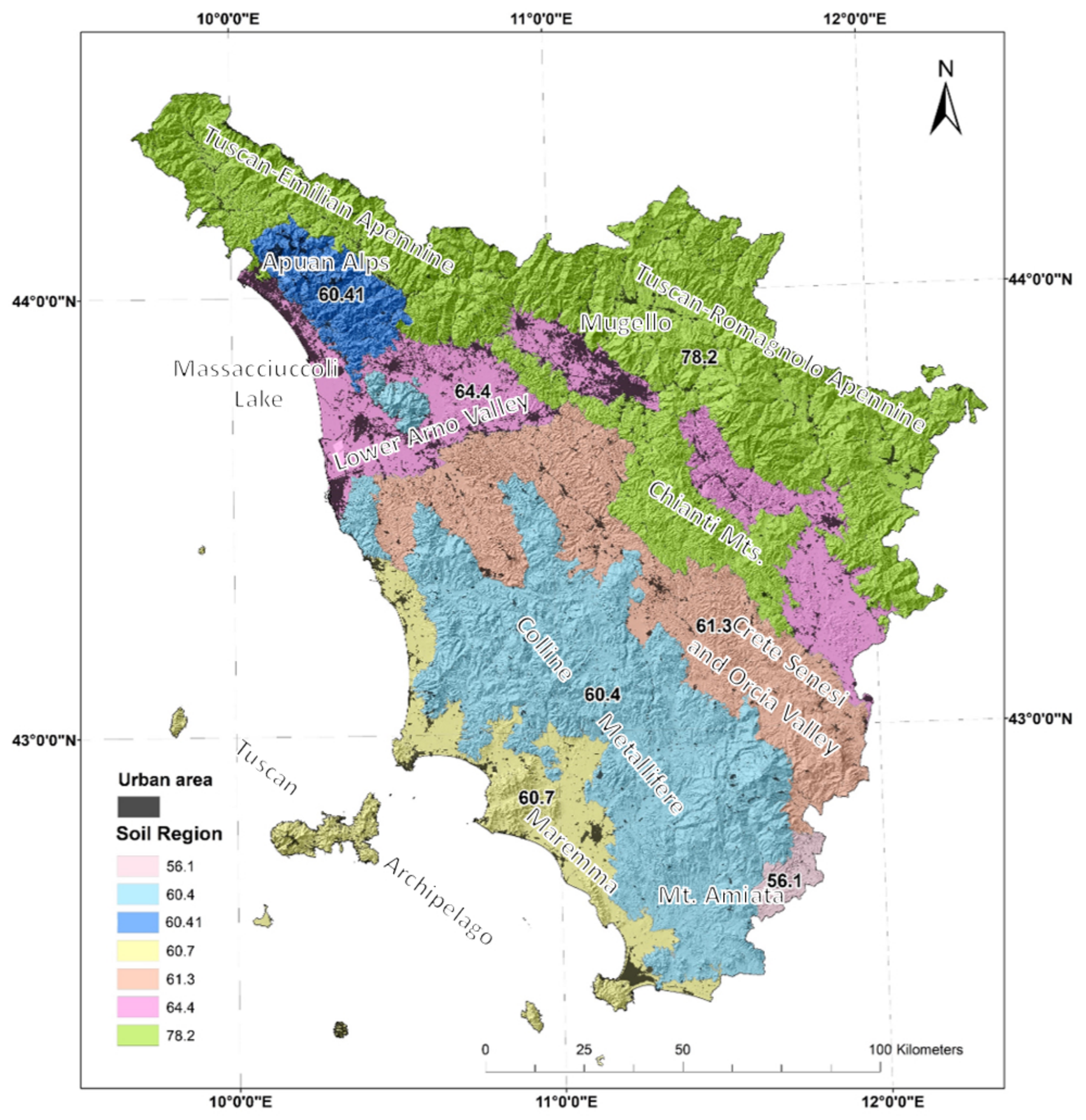
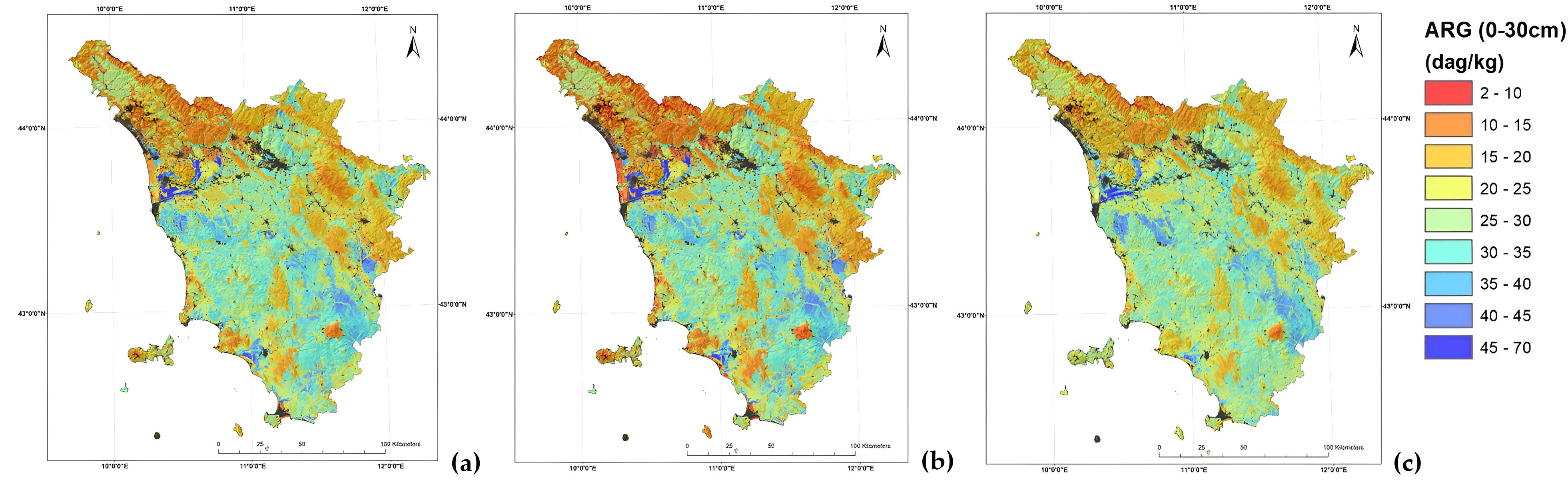
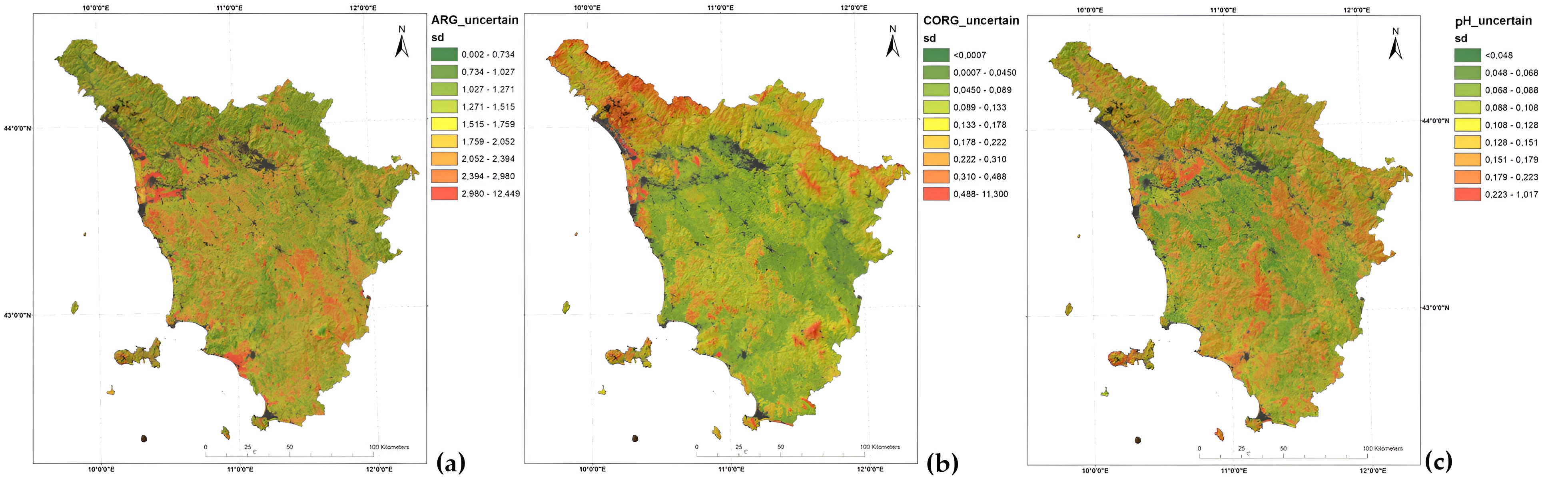
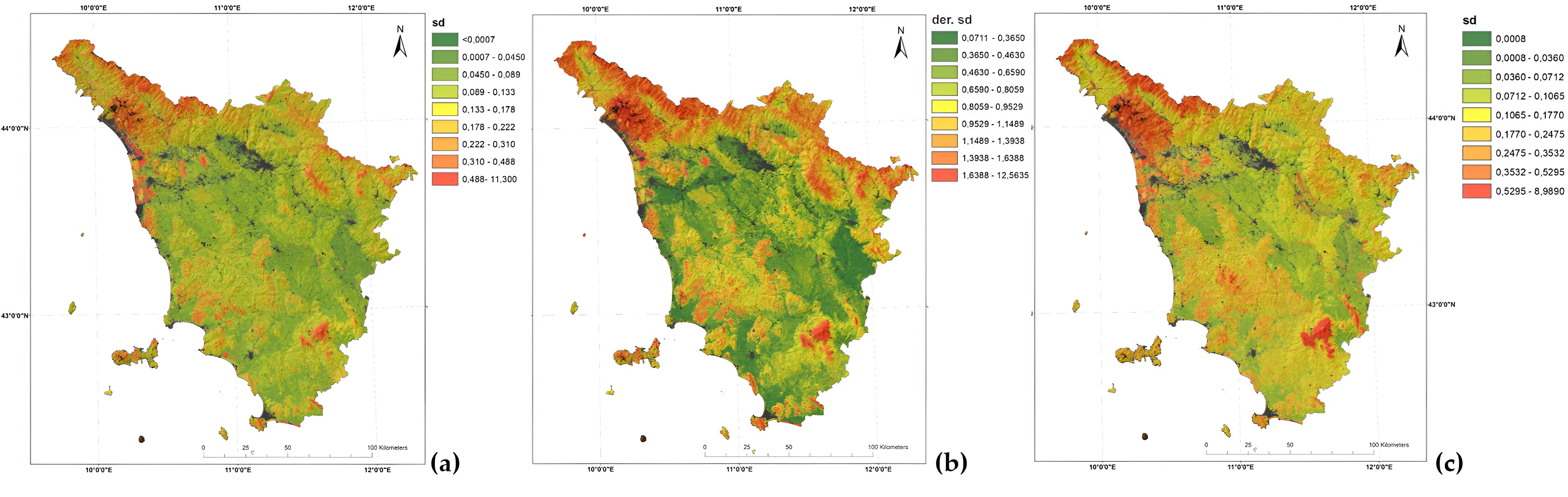

Disclaimer/Publisher’s Note: The statements, opinions and data contained in all publications are solely those of the individual author(s) and contributor(s) and not of MDPI and/or the editor(s). MDPI and/or the editor(s) disclaim responsibility for any injury to people or property resulting from any ideas, methods, instructions or products referred to in the content. |
© 2026 by the authors. Licensee MDPI, Basel, Switzerland. This article is an open access article distributed under the terms and conditions of the Creative Commons Attribution (CC BY) license.