


Abstract
The evolution of metropolitan transportation networks is an integral component of urban development. Policymakers are eager to prioritize sustainable development as their cities grow and progress. As such, academics have heavily turned their attention to the impact of providing more accessible public transportation, while significantly less academic work focuses on the reduction of public transportation accessibility. Our paper aims to contribute to the research gap surrounding bus stop consolidation. Public transportation efficiency theory posits that some bus stops with limited ridership should be consolidated with higher-demand stops. This paper evaluates the impact of bus stop consolidation on residents in Denver, Colorado by examining the effect of a consolidation project on surrounding residential property values from 2002 to 2022. We use a complete geospatial dataset of property values and bus stop closures during this two-decade span. Our project extends previous research by leveraging variation in the timing of the bus stop consolidations within a stacked spatial difference-in-differences model. Under the parallel trends assumption, we find the following results: (1) Houses that experience an above-median increase, greater than 151 m, in the distance to their nearest bus stop see their housing prices decline by approximately 3.6%. (2) The estimated decline is larger for closures occurring in or after 2017, a difference that is suggestive but not statistically significant. (3) The estimated decline is largest immediately following closure, with smaller point estimates in subsequent years. Although our research design provides evidence consistent with a housing-price response to bus stop closures, contemporaneous neighborhood changes may also contribute to the estimated effect.
1. Introduction
In 2022, bus service accounted for 48% of all public transportation trips in the United States [1]. Providing convenient access to this service requires transit agencies to make decisions about the number and spacing of stops along their routes. More frequent stops can reduce walking distances for riders but increase operating costs and travel-time delays. One way to manage this tradeoff is to consolidate stops, reducing the time buses spend stopping and accelerating while requiring some residents to walk farther to access the network. Although researchers have extensively examined the benefits of expanding public transportation, considerably less is known about the consequences of reducing local transit access. This paper examines how bus stop closures are reflected in nearby housing values.
Denver’s Regional Transportation District (RTD) provides a setting for studying this question. RTD has consolidated bus stops over several decades and, in 2017, renewed these efforts through an initiative targeting a 20% reduction in the number of stops [2,3]. The agency prioritized the closure of stops with low ridership, stops located less than one-quarter mile from another stop, and stops presenting safety concerns [2].
Using a spatially rich dataset on home sales in Denver, Colorado, we employ a spatial difference-in-differences design to estimate how reductions in bus stop accessibility are reflected in nearby home values. Our approach follows the hedonic revealed-preference literature, which uses housing prices to infer the value residents place on non-market amenities such as transit access [4,5,6,7]. For each bus stop closure, we compare home sales within 300 m of the closed stop with another set of sales within 300 m of a surviving active stop located within 2500 m of the closure. These properties had similar access to bus service before the closure, but only those near the closed stop experienced an increase in distance to the nearest active stop. Interpreting the resulting estimates as causal requires that, absent the closure, home prices near the closed stop would have evolved similarly to those near surviving stops. Because RTD prioritized low-ridership stops for closure, closures may coincide with neighborhood changes that also affect home prices. Although we assess pre-closure price trends to evaluate the plausibility of this assumption, we cannot rule out such changes.
Bus stop closures may increase nearby home values if consolidation reduces in-vehicle travel times or negative externalities associated with buses stopping and accelerating, such as noise and air pollution. Alternatively, home values may decline if residents place greater value on convenient access to the bus network and the closure increases the distance they must walk to reach a surviving stop. This additional walking time may be particularly costly in Denver during periods of extreme heat, cold, or snowfall [8]. Our estimates capture the net effect of these competing changes on housing values and do not isolate the contribution of any individual channel.
Under the parallel trends assumption, we find evidence that home values decline when bus stop closures substantially reduce access to the bus network. Specifically, we estimate that home prices are approximately 3.6% lower following a closure when the network distance to the nearest active stop increases by more than the sample median increase of 151 m. We find no statistically significant effect for smaller increases in distance. This finding is consistent with reductions in local transit accessibility being capitalized into nearby housing values.
Our study contributes to the literature on public transportation accessibility and housing values. Much of the existing research examines expansions in transit infrastructure or differences in access across locations [9,10,11,12,13]. A smaller literature examines housing-market responses to reductions in other forms of transportation infrastructure, including subway, rail, and airport closures [4,6,14,15]. Other work studies broader local effects of reductions in rail service and temporary rail-station closures [16,17,18,19]. We extend these literatures by examining the housing-market effects of individual bus stop closures, which represent localized reductions in transit accessibility rather than the removal of an entire transportation facility or service. Our findings suggest that the housing-market consequences of consolidation depend on how much a closure increases the distance to the nearest surviving stop.
Because our analysis focuses on Denver, the magnitude of our estimates may not generalize to other settings. Denver is a medium-sized and relatively young U.S. city with a developing transit system [20]. Effects may differ in cities with substantially different transportation systems, urban form, or preferences for public transit.
This paper proceeds as follows. Section 2 reviews the literature on hedonic valuation and public transportation. Section 3 describes the study area, data, and methods. Section 4 reports the results and robustness exercises. Section 5 presents the limitations and external validity, while Section 6 concludes with policy implications, data limitations, and directions for future research.
2. The Existing Literature and Policy Background
2.1. Land Rent Theory and Hedonic Evaluation
There is a wealth of academic literature examining the economic impacts of increased public services, surrounding public transportation. Many of these papers use changes in housing values to evaluate the benefit consumers place on public transportation. The idea that housing values can be used to approximate the value that consumers place on location-based amenities stems from land-rent theory as defined by Alonso [21], who associates the price of land with the corresponding ease of access to the desired amenities of the city center.
Other characteristics of houses also play a role in determining a parcel’s value, as noted by Muth [22]. Housing prices are determined by the aggregate value of a bundle of characteristics. Therefore, changes to this value can be analyzed to reveal the implicit value of location-specific amenities such as transit accessibility. Under this framework, housing prices should increase when local public transportation provides benefits that residents value and decrease when changes reduce the value of the location.
The theoretical contributions of Muth [22] were developed into an empirical approach by Lancaster [23] and Rosen [24]. Hedonic valuation uses housing transactions to provide information about willingness to pay under the usual hedonic framework assumptions. In our paper, we use the hedonic approach developed by Rosen [24] to examine how changes in bus stop accessibility are reflected in housing prices.
2.2. Expanded Public Transportation and Housing Values
Land rent theory and hedonic valuation have been used to analyze the value that consumers place on expanded access to various types of public transportation, including highways [25], heavy rail [26], and bus rapid transit systems [7,27,28]. Reviews by Mulley and Tsai [10], Yang et al. [29], Wang and Levinson [5], and Mann and Levinson [7] summarize this broader literature. In this study, we focus specifically on the effect of bus stop accessibility on housing values.
There is a smaller literature examining the relationship between bus stop accessibility and housing values. The literature has not reached a consensus regarding this question. Some papers find a positive relationship between bus stop accessibility and housing values [11,12,13,27,29,30,31]. For example, Yang et al. [31] finds that the number of nearby stops and the travel time to the city center are positively captured in housing values and Liu et al. [12] finds a varying impact of bus stop distance on rents, with a peak impact happening between 500 and 900 m of a bus stop. Others have found weak or statistically insignificant impacts of bus stop accessibility [27,32,33,34,35,36,37]. These seemingly contradictory findings may reflect differences in preferences for public transportation and other observables such as transit systems and geography, as noted by So et al. [32], as well as differences in empirical methods across studies.
Importantly for our project, most of this literature examines a cross section of public transportation levels. This implies that authors are relating properties with different levels of bus stop accessibility, without necessarily observing any changes in the level of accessibility. These estimates provide supportive evidence that residents value bus stop accessibility, and our study builds on this literature by leveraging changes in bus stop accessibility resulting from bus stop consolidation.
BRT research provides additional evidence that there may exist a positive link between increased access to public transportation and increased housing values. Numerous studies provide evidence of this positive relationship between BRT system access and housing values [9,10,27,28,38,39,40,41]. BRT is different from traditional bus services because BRT buses have dedicated infrastructure, less interference from road traffic, and greater service capacity. These differences limit the extent to which we can extrapolate to traditional bus stop services.
Taken together, this literature on expanded bus stop accessibility provides evidence that improving accessibility may be capitalized into housing values. The magnitude and potential direction of this impact have been shown to vary across different factors. This also raises a related question: what happens to housing prices when this same transportation accessibility is reduced? The following subsection reviews the narrow literature on reductions in public transportation services.
2.3. Reduced Public Transportation Accessibility and Housing Values
While the literature provides evidence that improvements in transportation accessibility can increase housing values, considerably less is known about how housing values respond when transportation services are reduced or suspended. There exists a larger literature on other modes, such as heavy rail and airports [14,15,16,42].
The effect of reducing transportation services on housing values is theoretically ambiguous because a closure can simultaneously remove transportation benefits and negative externalities. Housing values may be reduced due to the loss of transportation access, employment access, or other amenities associated with public transportation. On the other hand, removing noise pollution, air pollution, and other negative externalities may put upward pressure on housing values. Several studies examining airport and railway closures find that housing values increase following the cessation of operations, consistent with the removal of negative externalities. Breidenbach et al. [42] finds that housing prices near Berlin-Tegel Airport in Germany declined when delays in the opening of Berlin-Brandenburg Airport extended Berlin-Tegel’s operations. Zheng et al. [43] finds that housing values increased following the relocation of Kai Tak Airport in Hong Kong, while Sohn and Kim [15] finds that housing values increased following the closure of a 6.3-km segment of railway connecting Seoul and Chuncheon in South Korea.
However, the net impact of these competing channels may vary across transportation modes and environments. Cohen et al. [4] finds that housing prices increased after the closure of Denver’s Stapleton airport, but attributes the increase primarily to an expansion of neighborhood amenities, including retail and parks, and demographic change rather than the reduction in noise or other negative externalities. In contrast, Mai [14] finds that the permanent closure of the low-traffic Beijing Nanyuan Airport reduced surrounding home values. Mai argues that transportation facilities can generate countervailing positive and negative externalities, such that the net effect of closure depends on which effects are most important to nearby residents. In the case of Nanyuan Airport, the loss of transportation access and associated economic activity may have outweighed the benefits of reduced negative externalities.
These competing effects are particularly relevant when considering reductions in conventional bus service. Unlike airports and heavy rail, conventional bus stops generally generate smaller negative externalities, while providing transportation access to nearby residents. Consequently, residents may place relatively greater weight on the loss of accessibility than on the removal of noise or air pollution. The empirical literature examining housing-value effects of reductions in light rail, BRT, or conventional bus service, however, remains sparse.
Brolinson [6] provides related evidence by looking at the announcement of the L-train suspension in New York. The author finds that local housing values declined following the 2016 announcement. This study differs from ours in both transportation mode and the temporary nature of the reduction. Passengers knew that the L-train would reopen after refurbishment, while bus stop consolidation represents a more permanent reduction in public transportation accessibility.
Our study contributes to this literature by examining whether the reduction in accessibility resulting from bus stop consolidation is reflected in nearby housing values.
2.4. Public Transportation and Economic Outcomes
Bus stop consolidation can affect economic and transportation outcomes beyond housing values. In particular, consolidation may create a tradeoff between system-level efficiency and localized accessibility. Removing stops may allow buses to travel faster, permit more frequent service, or reduce operating costs.
El-Geneidy et al. [44] studies bus stop consolidation but focuses on passenger activity and operating performance rather than housing values. Their results provide evidence that changes in bus stop spacing can affect the efficiency and ridership of bus services. Likewise, in Montreal, Diab et al. [45] finds that increasing the frequency and average speed of bus routes was instrumental in ridership gains. These findings suggest that concentrating bus services can improve bus system performance, though these improvements may come at the cost of accessibility for residents who lose their nearby stop.
Other research examines the broader consequences of changes in bus service. Li and Wyczalkowski [46] examines the termination of the C-Tran bus service in Clayton County, Georgia, and its effects on unemployment and poverty. The existing literature therefore identifies several potential consequences of bus service changes, but provides limited evidence on how localized changes in accessibility affect the economic value of nearby properties. Our study connects these strands of literature by examining whether the increase in walking distance resulting from bus stop consolidation is capitalized into housing values.
2.5. Denver Public Transportation Initiative
In its 2017 consolidation initiative, the Denver Regional Transportation District (RTD) aimed to strike a balance between ease of stop access and reduced IVT. In other words, RTD wanted to improve its performance and cost effectiveness by making its routes as simple and efficient as possible without increasing access times to the point where it would significantly impact customer behavior [47]. To accomplish this objective, RTD prioritized the elimination of stops that were underutilized, excessively close to other bus stops (defined as stops located less than one-quarter mile from another stop), or particularly unsafe [2].
To demonstrate the mutual benefits of bus stop consolidation for providers and customers, RTD cites El-Geneidy et al. [44] in its project proposal. Looking at changes concentrated on a specific test route, El-Geneidy et al. [44] finds that bus stop consolidation had no significant effects on passenger activity, but improved bus running times by nearly 6% in Portland, Oregon. Passenger activity, however, does not directly measure residents’ willingness to pay for changes in local transit accessibility. Rather than examining passenger activity on a single route, our study examines changes in housing values across multiple bus stop consolidation events and over a longer time period.
Denver has a rich history of public transportation initiatives. The city has invested in light rail infrastructure [48], bike lanes [49], BRT [50], and traditional bus routes [50]. This dedication to public transportation may be unique to Denver, and we discuss the external validity of our results in Section 5. The BRT system in Denver is limited, with only one route, the Flatiron Flyer, providing service to downtown Denver since 2016 [51]. This route is designed primarily for longer-distance commutes from Boulder, and it stops only twice in the area where our traditional bus stops are located. The introduction of this line is therefore unlikely to systematically impact our estimates across the entire city.
3. Materials and Methods
3.1. Study Area
Denver, Colorado, is a medium-sized city in the Western United States. It sits on the Eastern side of the Rocky Mountains, and is considered a “young” city. Denver has a population of approximately 740,000 people with a median per capita income of slightly more than $64,000 per year [20]. Further, the average commute time is 24.6 min and approximately 2% of work trips are taken via public transportation [20]. Among public-transit commuters, 65% of these trips are taken via bus [52]. We provide this background on the city to assist the reader with the appropriateness of extrapolating our results to other cities.
We focus on Denver, Colorado, as our study area for multiple reasons, the most prominent being that the city has explicitly undertaken the initiative to consolidate bus stops by 20%, with the hope of increasing their ridership and route efficiency [2]. Denver’s position as one of the fastest-growing cities in the United States also marks it as a location of great importance for study, as the development of Denver’s public transportation will be vital to the future welfare of the city as a whole [53].
Additionally, public transportation in Denver is popular and in-demand, with data from Denver’s RTD showing that annual boardings rose by 5.9% between 2022 and 2024 to a total of 65,230,065 [50]. This provides evidence that residents are likely to pay attention to changes to their local bus routes, a speculation supported by Koutsopoulos [11], who found that increased bus stop accessibility was correlated with an increase in housing prices in 1970s Denver. Lastly, we chose Denver as our study location because the city has a long history of providing rich public spatial datasets, such as bus stops, bus routes, housing transactions, and parcel characteristics.
Figure 1 shows the location of the bus stop lines as well as light rail systems in this city. The parcel data are for the City of Denver, though the bus lines span a larger distance. We note that this is why there are many bus closures that are not included in our study due to the parcel data restriction. Nevertheless, there is a rich spatial variation to our data, in addition to the breadth of its temporal aspect, which spans approximately two decades.
Figure 1.
Denver, CO Bus routes. Author constructed GIS maps from RTD spatial shapefiles. Local and regional routes are bus stop routes. Software used: ArcGIS Pro version 3.5.0.
For our analysis, we provide baseline estimates and then test for temporal heterogeneity around 2017. This period coincides with the formalization of RTD’s standard for bus stop planning and consolidation along with a broader expansion in riders’ access to real-time transit information. Because these changes occurred at approximately the same time, we treat 2017 as a descriptive period break rather than attempting to isolate the effect of any single change. We discuss these developments and motivate the 2017 period split in Section 4.2.
3.2. Data
Data were obtained from the RTD Open Spatial Data repository [54] and the Denver Open Data Catalog [55]. RTD is the regional agency that operates public transit services in eight out of the twelve counties in the Denver-Aurora-Boulder Combined Statistical Area in the U.S. state of Colorado. We used a comprehensive file of past and present bus stops. From the Denver County Open Data website, we utilized arm’s-length property sales as well as parcel data that contained housing characteristics.
Through correspondence with Denver RTD, we obtained a roster of active and inactive bus stops as of 14 April 20231. For each stop, the file reports its address, unique RTD stop identifier, and the last date on which the stop was used. We link these records to an RTD-provided spatial dataset using the unique stop identifier, allowing us to identify the geographic locations of both active and inactive stops. We use these locations to calculate changes in network distance to the nearest active stop following a closure. We define a stop closure as the permanent deactivation of a bus stop after all routes serving that location cease to operate from it. Reductions in service do not constitute closures and are not identified in our data. If one or more routes continue to serve the stop, RTD records the stop as active.
Closure dates are defined by the last date on which a stop was used while all active bus stops show the same last used date, reflecting usage as of 14 April 2023. Stop closure announcements follow a standard public process in which RTD posts notice at the affected stop and gives riders six weeks to raise concerns before the change is finalized [2]. The most recent wave of inactive stops in the file dates to January 2023. Because our research design requires home sales both before and after a closure, the closures included in the analysis span 2002 to 2020. This restriction also ensured that each stop classified as closed had remained inactive for multiple years by the time the data were obtained, reducing the likelihood that temporary disruptions, such as construction-related closures, were included. RTD maintains its bus stop records using the General Transit Feed Specification (GTFS), in which each stop is assigned a unique identifier associated with a geographic location. However, observed inactivity does not rule out the possibility that some stops were relocated rather than permanently removed2.
Under our baseline model, the final stacked sample contains 501,340 observations drawn from 41,522 unique home sales. This sample includes home sales occurring within 2500 m of a bus stop closure, within three years before or after the closure, and within 300 m of a bus stop. A single sale can be linked to more than one nearby closure, serving as a control for each, so it may appear multiple times in the stacked sample. As a result, the number of stacked observations exceeds the number of unique sales. Table 1 reports the resulting observation counts of the stacked sample before and after closure and for treated and control units.
Table 1.
Summary Statistics and Within-Cohort Differences in Home Characteristics.
In Table 1, we report the summary statistics for the stacked sample of home sales described above. We provide information on the house, such as lot size, number of bedrooms, number of bathrooms, age, and living area, all characteristics that are included in our regression. Additionally, we show the sale price. We report these characteristics both before and after the closure. Column 1 reports the mean among control units, with column 2 reporting the mean among treated units. Finally, column 3 reports the coefficient from a regression of each characteristic on treatment status, controlling for cohort-by-year fixed effects, which tests whether treated and control units are statistically distinguishable within each cohort. We do find some statistically significant differences between treated and control homes after the closure, though the differences are economically small. Treated homes have 0.08 more bedrooms, about 55 more square feet of living area, and a lot size that is approximately 315 square feet larger than control homes.
One concern is that bus stop closures may change which homes are offered for sale, potentially conflating the estimated effect of closures with changes in the composition of transacting properties. The relatively small differences in observable characteristics provide some reassurance. We find that treated homes tend to have characteristics associated with higher, rather than lower, sale prices. Nevertheless, while our preferred specifications control for these observable differences, we cannot rule out selection into sales based on unobserved characteristics that may contribute to our estimated housing-price effects.
3.3. Empirical Methods: Stacked Event Study
We estimate the amenity value of bus stop access using a stacked event-study design. Each bus stop closure defines a cohort. Within a cohort, we compare home sales with reduced transit access due to the closure to nearby sales that continue to have access to a surviving bus stop. We then pool these cohort-specific comparisons into a single estimation sample.
To construct a cohort, we identify all home sales within 2.5 km of the closed stop and within three years of the closure date. We calculate distance as a network measure. Figure 2 provides a visual example of network distances. The example parcel noted by the blue outlines would be “snapped” to the closest road and then ArcGIS Pro version 3.5.0 calculates the distance along the road to the nearest bus stop, represented by a triangle for active stops or a red circle for an inactive stop. Euclidean distance would instead be calculated as a straight line from the parcel to the individual stops. Transportation empiricists favor network distance over Euclidean in a project such as this because pedestrians walk along streets rather than in straight lines, causing Euclidean distance to understate the actual distance residents must travel to reach a bus stop [56]. Accordingly, all distances used in the analysis refer to network distance.
Figure 2.
Denver, CO parcels and the associated bus stop locations. GIS was used to construct the network distance to the nearest inactive stop as well as the nearest active bus stops. Software used: ArcIGS Pro version 3.5.0.
Treatment status is defined relative to the stop that closes and anchors each cohort. A sale is treated if the property lies within 300 m of the closed stop and the closure increases its distance to the nearest active stop. A sale is a control if the property lies beyond 300 m of the closed stop, remains within 300 m of a different, surviving active stop, and experiences no change in distance to the nearest active stop. The within-cohort comparison is thus between nearby properties with similar initial transit access that differ in whether the closure reduces it. Figure 3 illustrates the construction of a single cohort.
Figure 3.
Cohort Design. (Note: Figure illustrates the construction of a single cohort in the stacked event-study design. The closed bus stop, shown in orange, defines the treated location. Surviving stops within 2.5 km of the closed stop, shown in blue, serve as cohort-specific control locations. The teal dashed circle denotes the 2.5-km cohort boundary. Treated sales are properties located within 300 m of the closed stop, while control sales are properties located within 300 m of an eligible surviving stop. The circular boundaries are schematic; all distance restrictions in the analysis are based on network distance rather than straight-line distance. The design is repeated separately for each closure cohort.)
Depending on whether a closure occurs in isolation or as part of Denver’s broader consolidation program, our treatment variable captures different underlying effects. An isolated, one-off closure primarily raises walking distance without meaningfully changing in-vehicle travel time on the route. But closures carried out as part of a systematic, network-wide consolidation effort, as in RTD’s post-2017 initiative, may also reduce in-vehicle travel time along the route, since removing stops can eliminate some deceleration, dwell, and re-acceleration time. For closures of this kind, our treatment variable captures the net effect of two opposing forces, increased access time and decreased in-vehicle time. A resident could in principle see a net decrease in total door-to-door travel time even if their measured distance to the nearest stop increases. In Section 4.2, we examine whether the estimated effect differs during the post-2017 period of more intensive consolidation.
The stacked design addresses a well-known limitation of two-way fixed-effects event studies with staggered treatment timing, in which units treated earlier serve as controls for units treated later [57]. When treatment effects evolve over time or differ across cohorts, these comparisons contaminate the event-time estimates even if untreated outcomes satisfy parallel trends [58,59]. We avoid these comparisons by constructing each cohort as a separate treated-control sample [60]. Within each cohort, treated units are compared only with units that remain untreated throughout the event window, so previously treated units never serve as controls.
Equation (1) outlines the primary event-study estimation:
Here i indexes a home sale observed at calendar date t, d indexes the closure cohort, and s indexes the bus stop to which sale i is assigned within cohort d, defined as the nearest stop that was active immediately before the focal closure. Each cohort has a closure date , and event time measuring time relative to that closure. Sales occurring during the year immediately before the closure are assigned to , and sales during the first year after the closure to . We estimate effects for between and 2, with serving as the omitted reference period. The vector contains hedonic characteristics of the property3. The term denotes nearest-stop-by-cohort fixed effects, which absorb time-invariant price differences across stop catchment areas within a cohort. The term denotes cohort-by-year fixed effects, which absorb market conditions and common shocks affecting all sales in a cohort at a given date.
Each coefficient measures the difference in log sale prices between treated and control properties at event time , relative to the corresponding difference in the year immediately preceding the closure. The coefficients and test for differential price movements before the closure, while through measure post-closure effects. Conditional on nearest-stop-by-cohort and cohort-by-year fixed effects, the identifying variation comes from within-cohort differences in price growth between properties near the closed stop and properties near surviving stops at each event time, relative to the year just before closure.
Interpreting the post-closure coefficients as causal requires the standard parallel trends assumption, namely that treated properties would have followed the same price path as controls absent the closure. Although this assumption cannot be tested directly, small and statistically insignificant pre-closure coefficients provide supporting evidence for its plausibility. If buyers anticipate the stop closure, estimates would be referenced to a partially treated period, attenuating our results. Because RTD gives riders approximately six weeks’ notice, there is some risk of this, though it is confined to a small share of the twelve-month reference period.
Valid inference on the estimates must account for two sources of correlation in the errors. First, unobserved pricing shocks may be correlated across sales sharing the same nearest-stop catchment, so treating these observations as independent could understate the standard errors. Second, because cohorts are constructed independently, the same transaction may appear in multiple cohort-specific samples, often as a control for several nearby closures. We therefore two-way cluster standard errors by nearest bus stop and individual home sale, allowing for dependence within stop catchments and across repeated appearances of the same transaction4.
Throughout much of the analysis, we pool the post-period effects into a single coefficient as shown in Equation (2).
Here, and interact treatment status with indicators for the corresponding pre-closure event periods, while equals one for treated observations in event periods . The coefficient measures the pooled treatment effect over the three post-closure periods, relative to the year immediately preceding the closure.
As a complementary check on parallel trends, we estimate a differential pre-period trend using only sales that occur before the closure.
In Equation (3), captures the difference in the linear pre-closure price trend between treated and control properties. An estimate near zero provides no evidence of a systematic differential linear trend during the three years preceding closure.
Lastly, a bus stop closure does not affect all nearby homes equally. For some properties the closure meaningfully reduces transit access, while for others the nearest surviving stop is only marginally farther away. To account for this variation in treatment intensity, we follow the continuous-treatment framework of Callaway et al. [61] and estimate effects separately for sales experiencing small and large increases in distance to the nearest stop.
3.4. Threats to Identification
The identifying assumption is that, absent the closure, home prices near stops that closed would have evolved similarly to those of nearby properties assigned to the comparison group. Verifying this assumption directly would require analyzing treated properties in the counterfactual world where their stop did not close, an outcome we can never observe. We instead rely on the pre-closure trend as evidence of plausibility. It is important to be explicit about why this evidence is supportive rather than conclusive, and about the specific channels through which it could fail even when the standard pre-trend tests we report show no evidence of differential trends.
A stacked DID does not require that closures be assigned independently of all characteristics. The concern is whether closures coincide with other changes that could differentially affect nearby treated and control properties. If they do, our estimates may conflate changes associated with the closure with the effect of whatever else was happening at the time. The simplest version of this is the classic DID violation: stops closing in neighborhoods where home prices were already on a declining trajectory, for reasons that have nothing to do with the stop itself. Two subtler versions of the same problem are worth naming directly, since both plausibly relate to RTD’s actual closure criteria.
RTD does not close stops at random but instead identifies stops with low ridership or substantial overlap with nearby service. Low ridership could itself signal changing neighborhood conditions, such as population loss or declining housing demand, that also place downward pressure on home prices. It could also reflect land-use change, such as a nearby rezoning, an employer’s relocation, or a redevelopment, which can reduce ridership at a stop and shift nearby prices for reasons that have nothing to do with the stop itself.
We do not observe annual neighborhood-level demographics, so we can not formally test these channels. One benefit of our research design is that we draw comparisons based on proximity, requiring controls to be within 2.5 km of the closure. The threat then becomes more specific: the underlying shock would need to affect the area around the treated stop without similarly affecting comparison properties elsewhere within the same 2.5-km cohort, which is a narrower concern. We cannot rule this out directly, but we can examine pre-period price trends for evidence that treated and comparison properties were already evolving differently before the closure.
The tradeoff of proximity-based controls is that closures could indirectly affect homes assigned to nearby active stops. Specifically, if displaced riders shift to a nearby active stop, this could change passenger volumes, crowding, service frequency, traffic, or investment in stop amenities at that location. These changes could in turn affect home prices near the surviving stop as well, meaning that some control properties may be partly affected by the closure, which could bias the estimated effect. As a robustness exercise, we later report estimates excluding control homes whose nearest active stop is located within 500 m of the closure.
4. Results and Discussion
4.1. Baseline Results
Our results are summarized in Table 2. Statistical inference throughout is based on two-sided tests using standard errors two-way clustered by nearest active bus stop and home sale ID. Across all specifications, the Treated × Prior terms, our pre-trend test, are not statistically significant, providing no evidence of differential pre-closure trends. However, the absence of differential pre-closure trends does not fully rule out the possibility that localized shocks coinciding with a bus stop closure differentially affected nearby treated and control properties. We begin with Column (1), which estimates our naive stacked difference-in-differences specification in Equation (2) and, under the parallel trends assumption, captures the average post-closure difference between treated and comparison properties. The coefficient of interest is the interaction term, Treated × Post, which is not statistically significant. Note that, this pooled estimate may mask heterogeneity associated with the dose of treatment. Homeowners may see little effect on their home’s value if an active stop remains within a short walk, while homeowners facing a substantially longer walk to the nearest remaining stop may experience a larger effect.
Table 2.
Impact of Bus Stop Distance Increase on Property Prices.
Column (2) tests this possibility directly by interacting the post-treatment effect with an indicator for high-dose treatment, defined at the property level as an increase in distance to the nearest active stop greater than the median of 151 m. The overall distribution of treatment dose is shown in Figure 4, with our cutoff highlighted by a vertical red line. Under our parallel trends assumption, the baseline treatment coefficient in Column (2) indicates a 1.2% decline in housing values among low-dose homes, a decline that is not statistically significant at conventional levels. The interaction coefficient indicates that high-dose homes experience an additional 2.2% decline relative to low-dose homes, with this difference statistically significant at the 5% level5.
Figure 4.
Cumulative Distribution of Treatment Intensity. (Note: Figure shows the cumulative distribution of increases in distance to the nearest active bus stop among treated homes between 2002 and 2022. The vertical red line corresponds to the treatment sample median distance of 151 m.)
Column (3) then restricts the treated sample to homes experiencing an increase greater than 151 m and estimates the total post-closure effect for these high-dose properties. Relative to the control group, their values decline by 3.6%, also statistically significant at the 5% level, equivalent to an increase of approximately $15,181 for the median-priced home. This estimate is similar in magnitude to the total high-dose effect of 3.3% obtained from the linear combination in Column (2), although the latter falls just short of statistical significance at the 5% level. Importantly, these estimated price effects capture the capitalized WTP of home buyers and owners, not resident welfare more broadly.
4.2. Temporal Heterogeneity After 2017
Between 2016 and 2017, Denver RTD introduced several changes relevant to bus stop access. RTD adopted formal service standards governing stop spacing and increasingly pursued systematic bus stop consolidation, while real-time transit information became more widely available to riders. Because these changes occurred at approximately the same time, our data do not allow us to isolate their separate effects. We therefore treat 2017 as a descriptive period break and test whether the housing-price response to closures differs for closures occurring in or after 2017.
One change during this period was the expansion of access to real-time transit information. Beginning in 2016, RTD made real-time vehicle-location and arrival-prediction data available to third-party applications [62]. In March 2017, RTD launched Next Ride, its own web-based application providing riders with real-time bus and light-rail arrival information. Thus, by 2017, riders had relatively broad access to real-time arrival information through both third-party services and RTD’s own platform. Figure 5 provides suggestive evidence that interest in Next Ride increased following its introduction. Google search activity for “Next Ride” rises sharply after 2017, while searches for “Bus Stop” remain comparatively stable. We view this pattern as consistent with growing public attention to RTD’s real-time information tools.
Figure 5.
Google Trends Search Term. (Note: Figure shows the monthly search term activity for Denver, Colorado. The search term popularity is normalized to 100 for the most searched term within the sample. The Next Ride app was introduced in March 2017.)
At approximately the same time, Denver RTD increasingly pursued systematic bus stop consolidation. RTD’s Transit Service Policies and Standards, approved in 2016, established stop-spacing guidelines and directed planners to consider pedestrian access, route travel time, ADA requirements, adjacent land uses, and streetscape conditions when locating stops [47]. By 2017, RTD explicitly described stop removals as part of an “ongoing bus stop consolidation program,” with stops targeted because of low usage or close proximity to adjacent stops [63]. Devunuri et al. [64] characterize this as a long-term consolidation initiative targeting a 20% reduction in stops and approximately quarter-mile spacing. Using historical GTFS data beginning in January 2017, they show that RTD’s traversal-weighted average stop spacing increased from roughly 378 m before the consolidation efforts to nearly 400 m by January 2020. These consolidations produced measurable travel-time savings, with RTD reporting that consolidating stops on the 0/0L saved riders approximately two minutes on average [3]. Consistent with this system-wide shift, Figure 6 shows a substantial increase in the pace of closures: 39% of closures between 2002 and 2022 occurred between 2017 and 2020 alone.
Figure 6.
Timing of Bus Stop Closures. (Note: Figure shows the cumulative share of bus stop closures by the Denver Regional Transportation District since 2003. The gray line includes all RTD closures, while the blue line includes closures used in the analysis. Closures are excluded when they cannot be linked to nearby property-sales data.)
More intensive consolidation could increase walking distances for properties affected by a closure while simultaneously improving travel times along surviving routes, as El-Geneidy et al. [44] find in a comparable Portland consolidation effort. At the same time, increasingly accessible real-time information may have changed how riders valued proximity to an active stop. Because these changes overlap, the pre- and post-2017 comparison cannot identify the effect of either mechanism separately. We therefore interpret the exercise as a test of temporal heterogeneity in the effect of bus stop closures.
To test whether the estimated effect differs during this later period, we interact the Treated × Post variable with an indicator for closures occurring in 2017 or later6. This interaction identifies the difference in the estimated post-closure effect between the later and earlier periods. Column (4) of Table 2 reports an imprecisely estimated interaction corresponding to a 2.5% additional decrease in home values for closures occurring in 2017 or later (). Column (5) restricts the sample to cohorts whose closure occurred in 2017 or later and estimates the effect directly within that period; here the estimated effect is a 4.1% decrease, statistically significant at the 10% level. Overall, we do not find robust evidence that the effect differs between the two periods, although the point estimates are suggestive of a larger decline for closures occurring in or after 2017.
4.3. The Impact of Substitutes on Consolidation
Another dimension of treatment heterogeneity is the availability of nearby active bus stops after a closure. The median treated home has one active bus stop within 300 m following the closure. Homes that remain close to multiple active stops may be less affected by the loss of any one stop, while homes with fewer nearby alternatives may experience a larger reduction in transit access.
We therefore test whether the estimated effect differs according to whether a treated home has one or fewer active bus stops within 300 m after the closure. Using the high-dose sample of closures occurring in 2017 or later, Column (6) of Table 2 interacts the post-closure treatment effect with an indicator for these homes. We find a statistically significant difference between homes with one or fewer nearby active stops and those with more than one. Homes with one or fewer active stops within 300 m have an estimated additional 8.5% decline in value following a closure relative to homes with more nearby alternatives, with the difference statistically significant at the 5% level.
4.4. Capturing Consolidation in the Market
Bus stop consolidation also raises the question of how quickly changes in access are reflected in housing prices. Figure 7 presents dynamic estimates from several specifications of our stacked event-study model. Across the panels, the pre-closure coefficients are statistically indistinguishable from zero, providing no evidence of differential pre-closure price trends.
Figure 7.
Stacked Event-Study Estimates of Bus Stop Closures and Home Prices. (Note: Figure shows dynamic treatment effects from the stacked event-study design. The top row includes closures from all years, while the bottom row restricts the sample to closures occurring from 2017 through 2020. The left-hand panels report estimates for closures that increase the distance to the nearest active bus stop by any amount. The right-hand panels separately report low-dose closures, which increase this distance by 151 m or less, and high-dose closures, which increase it by more than the treatment sample median, 151 m. Each point represents the estimated effect relative to the year immediately preceding the closure (). The outcome is the natural logarithm of the home sale price. All specifications control for property characteristics and include month, property-class, nearest-stop-by-cohort, and cohort-by-year fixed effects. Vertical bars show 95% confidence intervals based on standard errors two-way clustered by nearest bus stop and home sale.)
The top-left panel reports estimates for all closures regardless of treatment intensity. Consistent with Column (1) of Table 2, the post-closure coefficients remain close to zero and statistically insignificant. The bottom-left panel restricts the sample to closures occurring from 2017 through 2020 and shows a similar pattern.
The right-hand panels separate high- and low-dose closures. In both the full sample and the post-2017 sample, the post-closure point estimates are consistently more negative for high-dose closures. For these high-dose closures, the largest estimated decline occurs immediately following closure, with smaller negative estimates in the subsequent two years. Because the confidence intervals are relatively wide, we interpret this apparent attenuation as descriptive rather than evidence of a statistically distinct dynamic pattern.
Overall, the dynamic estimates are consistent with the pooled results in Table 2. The estimated housing-price response is concentrated among homes experiencing larger increases in distance to the nearest active stop, and the event-study estimates suggest that this response appears relatively quickly following closure. More broadly, our results indicate that the housing-market consequences of consolidation depend on the extent to which nearby transit access is reduced. Homes that remain close to alternative active stops experience smaller estimated declines, suggesting that the availability of nearby substitutes may mitigate some of the housing-market costs associated with a closure.
4.5. Robustness
We next examine the sensitivity of our main high-dose estimate reported in Column (3) of Table 2, which uses the full sample of closure cohorts, because there are multiple plausible values for each. This specification depends on three analyst choices: the high-dose cutoff, the stop catchment radius, and the cohort radius. In Figure 8, Figure 9 and Figure 10, Panel A reports the Treat × Post coefficient and Panel B reports from Equation (3), along with 95% confidence intervals. In each figure, the baseline specification is marked by a vertical red line.
Figure 8.
Sensitivity to the Treatment-Intensity Threshold. (Note: Figure shows how the estimated effects vary with the minimum increase in distance to the nearest active bus stop used to define treatment. At each value on the horizontal axis, the treated sample is restricted to sales near closures that increased the distance to the nearest active stop by more than the indicated number of meters; the control group is held fixed. (A) reports the coefficient on the interaction between treatment status and the post-closure period. (B) reports the differential linear pre-closure trend between treated and control sales. The red dashed line marks the treatment sample median, 151 m, which is used to define high-dose closures in the main analysis. The 300-m stop catchment, 2500 m cohort radius, and full sample of closure cohorts are held fixed throughout. All specifications control for property characteristics, and include month, property-class, nearest-stop-by-cohort, and cohort-by-year fixed effects. Shaded regions show 95% confidence intervals based on standard errors two-way clustered by nearest bus stop and home sale.)
Figure 9.
Sensitivity to the Catchment Radius: High-Dose. (Note: Figure examines how the estimated effects vary with the radius used to define each bus stop’s catchment area. At each value on the horizontal axis, the sample includes eligible sales located within the indicated distance of their pre-closure nearest stop. (A) reports the coefficient on the interaction between treatment status and the post-closure period. (B) reports the differential linear pre-closure trend between treated and control sales. The red dashed line marks the baseline catchment radius of 300 m. The 151-m high-dose threshold, 2500 m cohort radius, and full sample of closure cohorts are held fixed throughout. All specifications control for property characteristics, and include month, property-class, nearest-stop-by-cohort, and cohort-by-year fixed effects. Shaded regions show 95% confidence intervals based on standard errors two-way clustered by nearest bus stop and home sale.)
Figure 10.
Sensitivity to the Cohort Radius: High-Dose. (Note: Figure examines how the estimated effects vary with the geographic radius used to construct each closure cohort. At each value on the horizontal axis, eligible control stops are surviving stops located within the indicated distance of the closed stop. (A) reports the coefficient on the interaction between treatment status and the post-closure period. (B) reports the differential linear pre-closure trend between treated and control sales. The red dashed line marks the baseline cohort radius of 2500 m. The 151-m high-dose threshold, 300-m stop catchment, and full sample of closure cohorts are held fixed throughout. All specifications control for property characteristics, and include month, property-class, nearest-stop-by-cohort, and cohort-by-year fixed effects. Shaded regions show 95% confidence intervals based on standard errors two-way clustered by nearest bus stop and home sale.)
Figure 8 varies the high-dose cutoff used to define the treated sample, increasing the minimum required change in distance to the nearest active stop in 10-m increments. The estimated post-closure effect generally becomes more negative as the required increase in distance grows. Importantly, statistical significance is not unique to the 151-m cutoff. We find that 13 of the 25 alternative cutoffs above 50 m produce estimates statistically significant at the 5% level7.
Figure 9 varies the catchment radius used to assign parcels to treated and control stops. Smaller catchments restrict the sample to homes located closer to bus stops, where the stop is more likely to represent a relevant transit option, but they also reduce the sample size. As the catchment radius expands, increasingly distant homes are included and the estimated effect attenuates, consistent with weaker exposure to the closure among properties farther from the stop.
Finally, Figure 10 varies the radius used to construct each closure cohort. Smaller cohort radii provide more local comparison properties that may be more similar to treated homes and make the identifying assumption more local, since any confounding shock would need to differentially affect treated and comparison properties within a smaller geographic area. This comes at the cost of a smaller sample. Larger radii increase the number of available controls while potentially reducing their comparability to treated properties. Across cohort radii from 1500 to 5000 m, however, the estimated post-closure effect remains broadly similar, suggesting that the baseline result is not driven by the particular cohort radius we select.
The figures above address sensitivity to the analyst choices used to construct our main high-dose specification. Table 3 reports a second set of robustness checks addressing potential threats to identification and alternative sample and inference choices. All specifications use the full sample of closure cohorts and, unless otherwise noted, retain the baseline high-dose treatment definition. Column (1) reproduces the baseline estimate from Column (3) of Table 2. The first two rows report the pre-closure event-study coefficients, while Treated × Post reports the pooled post-closure effect of interest.
Table 3.
Robustness Checks for the Effect of Bus Stop Closures on Property Prices.
One concern is that properties in our comparison group may themselves be indirectly affected by the focal closure. In particular, displaced riders may substitute to surviving stops within a few minutes’ walk of the closed stop, potentially altering passenger volumes, service, traffic, or other characteristics around those locations. To address this concern, Column (2) reports a “donut” specification that excludes control properties whose assigned active stop is located within 500 m of the focal closed stop. The estimated post-closure effect is a 3.6% decline in home prices (), essentially unchanged from the baseline estimate (). Although this restriction reduces the potential for spillovers to nearby comparison properties, our estimates remain relative to homes near surviving stops that may themselves be affected by consolidation.
A second concern is anticipation. As discussed above, RTD provides approximately six weeks of notice before a proposed closure is implemented. If buyers or sellers respond to this announcement before the recorded closure date, transactions occurring shortly before the closure may already partially reflect the treatment. Because the year immediately preceding closure is our omitted reference period, such anticipation could attenuate or otherwise distort the estimated post-closure effect. Column (3) therefore excludes sales occurring during the six weeks immediately preceding the closure. The resulting estimate is a 3.6% decline in home prices (), falling just above the conventional 5% significance threshold but remaining very similar in magnitude to the baseline estimate.
We next examine whether our inference depends on the level at which standard errors are clustered. Our baseline specification two-way clusters standard errors by nearest bus stop and home sale, allowing for correlated pricing shocks among properties assigned to the same stop and for repeated appearances of the same transaction across closure cohorts. As an alternative, Column (4) clusters by closure cohort and home sale. The estimated post-closure effect remains 3.6%, with a standard error nearly identical to the baseline specification.
Finally, Columns (5) and (6) examine whether the results are driven by unusual observations or unusually small closure cohorts. Column (5) removes the top percentile of the treatment-dose distribution, reducing the influence of properties experiencing exceptionally large increases in distance to the nearest active stop. The estimated effect remains 3.6%. Column (6) removes closure cohorts in the bottom percentile of the cohort-size distribution, retaining only cohorts with more than 79 observations in the baseline sample. Again, the estimate remains similar at 3.3%. Across the specifications reported in Table 3, the estimated post-closure effect ranges from 3.3% to 3.6%, with p-values between 0.044 and 0.079. Although some estimates fall above the conventional 5% significance threshold, all remain statistically significant at the 10% level, and the point estimates are remarkably stable in magnitude across specifications. We view these results as providing little indication that the baseline estimate is driven by the proximity of nearby control properties, anticipation effects, the choice of clustering, extreme treatment doses, or unusually small cohorts.
4.6. Results in Context of the Literature
Compared with previous studies of bus stop accessibility and housing values, our estimated effect is relatively large. Under the parallel trends assumption, we find that bus stop closures are associated with a 3.6% decline in housing values among homes experiencing an above-median increase in distance to the nearest active stop. By comparison, previous studies that find a positive relationship between bus stop accessibility and housing values generally estimate increases of only 0.03% to 0.5% [11,29,30,31]. Our estimated magnitude is closer to the capitalization effects found in studies of bus rapid transit systems, where changes in transit access tend to produce larger housing-market responses [9,10,41]. Although studies of expanded and reduced accessibility are not directly comparable, both examine how changes in transit access are reflected in housing values. If gains and losses in bus stop accessibility were valued symmetrically, one might expect effects of roughly similar magnitude. Our estimate is substantially larger, suggesting that the housing-market response to losing nearby access may differ from the response to gaining it. Alternatively, the difference may reflect characteristics specific to the Denver housing and transit market rather than a general asymmetry in how households value gains and losses in bus stop access.
One speculative explanation for the larger coefficient in our study is that expansions in bus stop access may occur in areas where residents already have several nearby alternatives. If so, adding another stop may produce only a small reduction in distance to the nearest stop and therefore a relatively small change in housing values. A second possibility comes from loss aversion, as households may respond more strongly to losing nearby transit access than to an equivalent gain in access [65]. Finally, many of the studies cited above rely on cross-sectional variation in bus stop accessibility, while our estimates use changes in access surrounding stop closures. Differences in research design and identifying variation may therefore also contribute to the difference in estimated magnitudes.
4.7. Policy Discussion and Travel Time Trade-Off
Our results highlight an important tradeoff in bus stop consolidation. Removing stops can increase the distance that some residents must travel to access the bus network, while at the same time reducing in-vehicle travel time by cutting the number of stops along a route. Previous work has shown that bus stop consolidation can improve route performance and reduce travel time [44,66]. Our data directly measure changes in distance to the nearest active stop, but do not allow us to separately measure changes in the in-vehicle travel time associated with each closure.
To provide some economic scale for the walking-distance component of this tradeoff, we offer a simple back-of-the-envelope calculation. An increase of approximately 150 m in network distance corresponds to roughly two additional minutes of walking each way at a typical walking pace. The U.S. Department of Transportation estimates the value of travel-time savings for business travelers at $25.40 per person-hour in 2016, equivalent to approximately $27.66 in 2020 dollars [67]. Applying this value to an additional two minutes of walking in each direction, five days per week for 50 weeks per year, implies an annual time cost of approximately $461. Capitalized in perpetuity at a 5% discount rate, this corresponds to roughly $9220. This illustrative calculation isolates the additional walking time and is not intended to account for the other changes associated with a bus stop closure.
This distinction is important for transportation planners. We find that the estimated decline in housing values is concentrated among homes experiencing larger increases in distance to the nearest active stop, while closures that leave homes relatively close to another active stop have much smaller estimated effects. This suggests that the housing-market costs associated with consolidation may depend importantly on the extent to which a closure reduces nearby transit access. When selecting stops for consolidation, planners may therefore want to consider not only potential improvements in route efficiency but also the additional distance imposed on residents around the closed stop.
More generally, our results do not imply that bus stop consolidation reduces overall welfare. Faster travel times, improved reliability, lower operating costs, and other benefits may offset some or all of the losses associated with reduced stop access. Our estimates capture one margin of this tradeoff through housing prices and should be considered alongside these other potential costs and benefits when evaluating consolidation policies.
5. Limitations and External Validity
Our research design relies on the assumption that, absent a bus stop closure, housing prices near stops that closed would have evolved similarly to those of nearby comparison properties. As discussed in Section 2.5, RTD did not select stops for closure at random, and factors such as low ridership or changes in neighborhood conditions could be related both to closure decisions and to housing prices. Our proximity-based comparison groups, pre-closure trend tests, and robustness exercises help address these concerns, but they cannot fully rule out localized shocks that occur contemporaneously with a closure. Additionally, closures could influence which properties are offered for sale, potentially introducing selection based on unobserved housing characteristics for which our empirical specification cannot account. Our estimates should therefore be interpreted subject to these limitations.
A second limitation concerns the external validity of our results. Denver has made sustained investments in public transportation for several decades, including bus service, light rail, and other transit infrastructure [50]. Previous work has also found evidence that bus stop accessibility is reflected in Denver housing values [11]. These features may mean that households with stronger preferences for transit access are more likely to locate in Denver, in the spirit of Tiebout sorting in which households select communities partly on the basis of the public services and amenities they provide [68]. If so, changes in bus stop accessibility may be capitalized more strongly into Denver housing values than they would be in markets where transit plays a less prominent role. The magnitude of our estimates may therefore not generalize to cities where bus transit is less central to local transportation or less highly valued by residents.
Finally, our analysis covers bus stop closures over a long period, and the housing-market response to changes in transit access may vary over time. Housing-market conditions, transit usage, service quality, and residents’ valuation of bus access can all change across periods. As a result, the magnitude of the effects we estimate in Denver from 2002 to 2022 may not generalize directly to closures occurring under different economic or transit-policy conditions.
6. Conclusions
A substantial literature has examined the effects of increasing access to public transportation, including expansions in light rail [69], bus and bus rapid transit systems [9,10,41], and heavy rail [70]. We instead examine the less-studied case of decreasing public transportation access through bus stop closures. Denver, Colorado, provides a useful setting for this question because RTD has explicitly pursued bus stop consolidation, including an initiative targeting a 20% reduction in stops [2].
Our study examines one margin of the consequences of these closures: changes in nearby housing values. Under the parallel trends assumption, we find that bus stop closures are associated with a 3.6% decline in housing values among homes experiencing an above-median increase in distance to the nearest active stop. Although our pre-closure trend tests are consistent with this assumption, we cannot rule out the possibility that contemporaneous changes in neighborhood conditions contribute to the estimated effect. This estimated effect is relatively large compared with the estimates found in previous studies of expanded bus stop accessibility, which generally find increases in housing values of approximately 0.03% to 0.5% [11,29,30,31]. These estimates are not directly comparable, because the studies examine different changes in transit access, markets, and empirical settings. As discussed above, the difference in magnitude may reflect differences in research design, a stronger response to losing rather than gaining nearby transit access, or characteristics specific to the Denver housing and transit market.
The estimated decline in housing values is concentrated among homes experiencing larger increases in distance to the nearest active stop. We also find suggestive evidence that the estimated effect is larger for closures occurring during RTD’s more intensive period of bus stop consolidation, although the difference relative to earlier closures is not statistically significant. Our dynamic estimates indicate that the housing-market response occurs relatively quickly following a closure, with point estimates becoming less negative in subsequent years. These patterns suggest that both the size of the change in transit access and timing in which a closure occurs may matter for its housing-market consequences.
Bus stop consolidation therefore presents a tradeoff for transportation planners. Removing stops can increase the distance residents must travel to access the bus network, while fewer stops may also improve route performance and reduce in-vehicle travel time. Our estimates reflect the capitalization of these changes into housing prices and do not measure resident welfare more broadly. They nevertheless suggest that planners may want to consider the additional distance imposed on nearby households alongside potential improvements in route efficiency, reliability, and operating costs when evaluating bus stop consolidation.
Author Contributions
Conceptualization, E.C.-S. and K.J.B.; methodology, K.J.B. and D.K.; software, K.J.B. and D.K.; formal analysis, K.J.B. and D.K.; investigation, E.C.-S. and C.K.; resources, E.C.-S. and C.K.; data curation, K.J.B. and E.C.-S.; writing—original draft preparation, E.C.-S.; writing—review and editing, C.K. and D.K.; visualization, K.J.B. and D.K.; supervision, K.J.B.; project administration, K.J.B. All authors have read and agreed to the published version of the manuscript.
Funding
This research received no external funding.
Data Availability Statement
The original data presented in the study are openly available in Denver Open Data at https://opendata-geospatialdenver.hub.arcgis.com/ (accessed on 14 February 2023) and RTD Open Data at https://gis-rtd-denver.opendata.arcgis.com/ (accessed on 14 February 2023).
Conflicts of Interest
The authors declare no conflicts of interest.
Abbreviations
The following abbreviations are used in this manuscript:
| APTA | American Public Transportation Association |
| BRT | Bus Rapid Transit |
| IVT | In-vehicle Time |
| RTD | Regional Transportation District |
| WTP | Willingness to Pay |
| GTFS | General Transit Feed Specification |
Notes
| 1 | This file does not report the routes that historically served closed stops or the history of discontinued routes at stops that remain active. |
| 2 | Our dataset includes the locations of both active and inactive stops. Because we observe a single snapshot of the bus stop network, we cannot distinguish all relocations from permanent removals. Nevertheless, a relocation that increases a property’s distance to the nearest active stop represents a reduction in accessibility of the kind our treatment measure is designed to capture. |
| 3 | Property characteristics include lot size, above-ground living area, property age and its square, and the distance to the property’s nearest active bus stop immediately before the focal closure and its square, along with fixed effects for the number of bedrooms, number of full bathrooms, property class, and month of sale. |
| 4 | Clustering by closure cohort rather than nearest bus stop produces very similar standard errors. |
| 5 | The total effect for the high-dose group is given by the linear combination of the and coefficients. This estimated effect is , with a standard error of (). |
| 6 | Column (2) suggests that closures have little effect for homes that remain close to another active stop. To simplify the specification, rather than estimate separate interaction terms across treatment doses, we restrict the treated group to “high-dose” closures, defined as those that increase network distance to the nearest surviving stop by more than 151 m. |
| 7 | At the 10% level, 21 of the 25 alternative cutoffs are statistically significant. |
References
- APTA. 2024 Public Transportation Factbook. 2024. Available online: https://www.apta.com/research-technical-resources/transit-statistics/public-transportation-fact-book/ (accessed on 7 July 2026).
- Regional Transportation District (Denver, Colorado). RTD Bus Stop Consolidation Project Update, 2023. 2023. Available online: https://web.archive.org/web/20250524131651/https://www.rtd-denver.com/about-rtd/projects/busstop-consolidation (accessed on 27 March 2025).
- Sachs, D. Why RTD Is Consolidating Bus Stops. 2018. Available online: https://web.archive.org/web/20250524133220/https://denver.streetsblog.org/2018/01/29/why-rtd-is-consolidating-busstops/ (accessed on 26 August 2025).
- Cohen, J.P.; Coughlin, C.C.; Crews, J.; Ross, S.L. Longer term housing market effects of a major US airport closure. Real. Estate Econ. 2023, 51, 990–1010. [Google Scholar] [CrossRef] [Scilit]
- Wang, Y.; Levinson, D. Access-based land value appreciation for assessing project benefits. J. Transp. Land Use 2023, 16, 469–496. [Google Scholar] [CrossRef] [Scilit]
- Brolinson, B. Valuing public transit: The L-train shutdown. Real. Estate Econ. 2024, 52, 794–842. [Google Scholar] [CrossRef] [Scilit]
- Mann, I.; Levinson, D.M. Access for appraisal: A systematic review of estimating transport benefits via real-estate uplift. Transp. Rev. 2026, 46, 840–862. [Google Scholar] [CrossRef] [Scilit]
- U.S. Climate Data. Climate-Denver Colorado. 2026. Available online: https://usclimatedata.com/climate/denver/colorado/united-states/usco0105 (accessed on 8 July 2026).
- Dubé, J.; Des Rosiers, F.; Thériault, M.; Dib, P. Economic impact of a supply change in mass transit in urban areas: A Canadian example. Transp. Res. Part A Policy Pract. 2011, 45, 46–62. [Google Scholar] [CrossRef] [Scilit]
- Mulley, C.; Tsai, C.H.P. When and how much does new transport infrastructure add to property values? Evidence from the bus rapid transit system in Sydney, Australia. Transp. Policy 2016, 51, 15–23. [Google Scholar] [CrossRef] [Scilit]
- Koutsopoulos, K. The Impact of Mass Transit on Residential Property Values. Ann. Assoc. Am. Geogr. 1977, 64, 564–576. [Google Scholar] [CrossRef] [Scilit]
- Liu, Q.; Zhao, P.; Xiao, Y.; Zhou, X.; Yang, J. Walking Accessibility to the Bus Stop: Does It Affect Residential Rents? The Case of Jinan, China. Land 2022, 11, 860. [Google Scholar] [CrossRef] [Scilit]
- Liu, T.; Wang, J.; Liu, L.; Peng, Z.; Wu, H. What Are the Pivotal Factors Influencing Housing Prices? A Spatiotemporal Dynamic Analysis Across Market Cycles from Upturn to Downturn in Wuhan. Land 2025, 14, 356. [Google Scholar] [CrossRef] [Scilit]
- Mai, Y. When the Airport Falls Silent: Airport Closure and Housing Market Dynamics. J. Real. Estate Finance Econ. 2026, 73, 322–353. [Google Scholar] [CrossRef] [Scilit]
- Sohn, C.; Kim, G.H. How does railroad track closure affect housing values? The case of Seoul, Korea. Spat. Inf. Res. 2016, 24, 347–354. [Google Scholar] [CrossRef] [Scilit]
- Chan, J. End of the Line: The Effects of Large Passenger Rail Cuts on Local Economic Outcomes. Can. Public Policy 2024, 50, 422–439. [Google Scholar] [CrossRef] [Scilit]
- DeAngelo, G.; Gittings, K.; Grossman, D.S.; Khalil, U. Urban Transport and Crime: Evidence from Unanticipated Mass Transit Strikes. Econ. Inq. 2019, 57, 1718–1737. [Google Scholar] [CrossRef] [Scilit]
- Gibbons, S.; Heblich, S.; Pinchbeck, E.W. The spatial impacts of a massive rail disinvestment program: The Beeching Axe. J. Urban Econ. 2024, 143, 103691. [Google Scholar] [CrossRef] [Scilit]
- Phillips, D.C.; Sandler, D. Does public transit spread crime? Evidence from temporary rail station closures. Reg. Sci. Urban Econ. 2015, 52, 13–26. [Google Scholar] [CrossRef] [Scilit]
- US Census Bureau, U.C. Denver Quick Facts. 2016. Available online: https://www.census.gov/quickfacts/fact/table/denvercountycolorado/PST045225 (accessed on 22 July 2026).
- Alonso, W. Location and Land Use. Toward a General Theory of Land Rent; Harvard University Press: Cambridge, MA, USA, 1964. [Google Scholar] [CrossRef] [Scilit]
- Muth, R. Cities and Housing: The Spatial Pattern of Urban Residential Land Use; The Univerity of Chicago Press: Chicago, IL, USA; London, UK, 1969. [Google Scholar]
- Lancaster, K. A New Approach to Consumer Theory. J. Political Econ. 1966, 74, 132–157. [Google Scholar] [CrossRef] [Scilit] [PubMed]
- Rosen, S. Hedonic Prices and Implicit Markets: Product Differentiation in Pure Competition. J. Political Econ. 1974, 82, 34–55. [Google Scholar] [CrossRef] [Scilit] [PubMed]
- Murray, J.; Bardaka, E. Evaluating the spatial and temporal distribution of beltway effects on housing prices using difference-in-differences methods. Transportation 2022, 49, 1963–1998. [Google Scholar] [CrossRef] [Scilit]
- Mathur, S. Impact of transit stations on house prices across entire price spectrum: A quantile regression approach. Land Use Policy 2020, 99, 104828. [Google Scholar] [CrossRef] [Scilit]
- Zhang, B.; Li, W.; Lownes, N.; Zhang, C. Estimating the Impacts of Proximity to Public Transportation on Residential Property Values: An Empirical Analysis for Hartford and Stamford Areas, Connecticut. ISPRS Int. J. Geo-Inf. 2021, 10, 44. [Google Scholar] [CrossRef] [Scilit]
- Beaudoin, J.; Tyndall, J. The effect of bus rapid transit on local home prices. Res. Transp. Econ. 2023, 102, 101370. [Google Scholar] [CrossRef] [Scilit]
- Yang, L.; Zhou, J.; Shyr, O.F.; Huo, D.D. Does bus accessibility affect property prices? Cities 2019, 84, 56–65. [Google Scholar] [CrossRef] [Scilit]
- Wang, Y.; Potoglou, D.; Orford, S.; Gong, Y. Bus stop, property price and land value tax: A multilevel hedonic analysis with quantile calibration. Land Use Policy 2015, 42, 381–391. [Google Scholar] [CrossRef] [Scilit]
- Yang, L.; Chau, K.W.; Szeto, W.Y.; Cui, X.; Wang, X. Accessibility to transit, by transit, and property prices: Spatially varying relationships. Transp. Res. Part D Transp. Environ. 2020, 85, 102387. [Google Scholar] [CrossRef] [Scilit]
- So, H.M.; Tse, R.Y.; Ganesan, S. Estimating the influence of transport on house prices: Evidence from Hong Kong. J. Prop. Valuat. Invest. 1997, 15, 40–47. [Google Scholar] [CrossRef] [Scilit]
- Zheng, S.; Kahn, M.E. Land and residential property markets in a booming economy: New evidence from Beijing. J. Urban Econ. 2008, 63, 743–757. [Google Scholar] [CrossRef] [Scilit]
- Ibeas, Á.; Cordera, R.; Dell’Olio, L.; Coppola, P.; Dominguez, A. Modelling transport and real-estate values interactions in urban systems. J. Transp. Geogr. 2012, 24, 370–382. [Google Scholar] [CrossRef] [Scilit]
- Wen, H.; Zhang, Y.; Zhang, L. Do educational facilities affect housing price? An empirical study in Hangzhou, China. Habitat Int. 2014, 42, 155–163. [Google Scholar] [CrossRef] [Scilit]
- Wen, H.; Tao, Y. Polycentric urban structure and housing price in the transitional China: Evidence from Hangzhou. Habitat Int. 2015, 46, 138–146. [Google Scholar] [CrossRef] [Scilit]
- Wen, H.; Xiao, Y.; Zhang, L. School district, education quality, and housing price: Evidence from a natural experiment in Hangzhou, China. Cities 2017, 66, 72–80. [Google Scholar] [CrossRef] [Scilit]
- Rodríguez, D.A.; Mojica, C.H. Capitalization of BRT network expansions effects into prices of non-expansion areas. Transp. Res. Part A Policy Pract. 2009, 43, 560–571. [Google Scholar] [CrossRef] [Scilit]
- Deng, T.; Nelson, J. The impact of Bus Rapid Transit on land development: A case study of Beijing, China. World Acad. Sci. Eng. Technol. 2010, 66, 1196–1206. [Google Scholar]
- Munoz-Raskin, R. Walking accessibility to bus rapid transit: Does it affect property values? The case of Bogotá, Colombia. Transp. Policy 2010, 17, 72–84. [Google Scholar] [CrossRef] [Scilit]
- Cervero, R.; Kang, C.D. Bus rapid transit impacts on land uses and land values in Seoul, Korea. Transp. Policy 2011, 18, 102–116. [Google Scholar] [CrossRef] [Scilit]
- Breidenbach, P.; Cohen, J.; Schaffner, S. Continuation of air services at Berlin-Tegel and its effects on apartment rental prices. Real. Estate Econ. 2022, 50, 1548–1575. [Google Scholar] [CrossRef] [Scilit]
- Zheng, X.; Peng, W.; Hu, M. Airport noise and house prices: A quasi-experimental design study. Land Use Policy 2020, 90, 104287. [Google Scholar] [CrossRef] [Scilit]
- El-Geneidy, A.M.; Strathman, J.G.; Kimpel, T.J.; Crout, D.T. Effects of bus stop consolidation on passenger activity and transit operations. Transp. Res. Rec. 2006, 1971, 32–41. [Google Scholar] [CrossRef][Green Version]
- Diab, E.; DeWeese, J.; Chaloux, N.; El-Geneidy, A. Adjusting the service? Understanding the factors affecting bus ridership over time at the route level in Montréal, Canada. Transportation 2021, 48, 2765–2786. [Google Scholar] [CrossRef] [Scilit]
- Li, F.; Wyczalkowski, C.K. How buses alleviate unemployment and poverty: Lessons from a natural experiment in Clayton County, GA. Urban Stud. 2023, 60, 2632–2650. [Google Scholar] [CrossRef] [Scilit]
- Regional Transportation District (Denver, Colorado). Transit Service Policies and Standards. 2016. Available online: https://cdn.rtd-denver.com/image/upload/v1707247621/service-standards-7-2016_rg0fun.pdf? (accessed on 10 July 2026).
- Denver, R.T.D. Rail. 2026. Available online: https://www.rtd-denver.com/routes-services/rail (accessed on 8 September 2026).
- Department of Transportation and Infrastructure. Denver Moves: Safe and Slow Streets with Bikeways. 2026. Available online: https://www.denvergov.org/Government/Agencies-Departments-Offices/Agencies-Departments-Offices-Directory/Department-of-Transportation-and-Infrastructure/Programs-Services/Bicycles (accessed on 8 September 2026).
- Regional Transportation District (Denver, Colorado). RTD Facts and Figures. 2025. Available online: https://web.archive.org/web/20250807160127/https://www.rtd-denver.com/open-records/reports-and-policies/facts-figures (accessed on 26 July 2025).
- Denver RTD. Rail. 2026. Available online: https://www.rtd-denver.com/open-records/reports-and-policies/facts-and-figures/flatiron-flyer (accessed on 8 September 2026).
- US Census Bureau. Means of Transportation to Work. 2016. Available online: https://data.census.gov/table?q=b08301g=310XX00US19740 (accessed on 22 July 2026).
- Bartel, H. US News and World Report. 2025. Available online: https://web.archive.org/web/20250311213619/https://realestate.usnews.com/places/rankings/fastest-growing-places (accessed on 8 March 2025).
- Regional Transportation District. Open Spatial Data. 2026. Available online: https://www.rtd-denver.com/open-records/open-spatial-information (accessed on 14 April 2023).
- City and County of Denver. Denver Open Data Catalog. 2026. Available online: https://opendata-geospatialdenver.hub.arcgis.com (accessed on 14 April 2023).
- García, R.T.; Pérez Sánchez, R.; Lopez, M.F. A Comparative Analysis of Manhattan, Euclidean and Network Distances. Why Are Network Distances More Useful to Urban Professionals? In Proceedings of the Conference: 18th International Multidisciplinary Scientific GeoConference SGEM2018, Albena, Bulgaria, 30 June–9 July 2018. [Google Scholar] [CrossRef] [Scilit]
- Goodman-Bacon, A. Difference-in-differences with variation in treatment timing. J. Econom. 2021, 225, 254–277. [Google Scholar] [CrossRef] [Scilit]
- Callaway, B.; Sant’Anna, P.H. Difference-in-differences with multiple time periods. J. Econom. 2021, 225, 200–230. [Google Scholar] [CrossRef] [Scilit]
- Sun, L.; Abraham, S. Estimating dynamic treatment effects in event studies with heterogeneous treatment effects. J. Econom. 2021, 225, 175–199. [Google Scholar] [CrossRef] [Scilit]
- Wing, C.; Freedman, S.M.; Hollingsworth, A. Stacked Difference-in-Differences; Technical report; National Bureau of Economic Research: Cambridge, MA, USA, 2024. [Google Scholar]
- Callaway, B.; Goodman-Bacon, A.; Sant’Anna, P.H.C. Event Studies with a Continuous Treatment. AEA Pap. Proc. 2024, 114, 601–605. [Google Scholar] [CrossRef] [Scilit]
- Burness, A. This Change Means Less Time Spent at Bus Stops. Denver7. 2016. Available online: https://www.denver7.com/news/local-news/rtd-releases-data-for-real-time-app-tracking-of-denver-area-buses (accessed on 9 September 2026).
- Regional Transportation District (Denver; Colorado). Proposed Service Changes for January 2018. Operations and Customer Service Committee, Board of Directors, 8 August 2017. Reproduced by the National Federation of the Blind of Colorado. 8 August 2017. Available online: https://nfbnet.org/pipermail/colorado-talk_nfbnet.org/2017-August/003150.html (accessed on 28 July 2026).
- Devunuri, S.; Lehe, L.J.; Qiam, S.; Pandey, A.; Monzer, D. Bus Stop Spacing Statistics: Theory and Evidence. J. Public Transp. 2024, 26, 100083. [Google Scholar] [CrossRef] [Scilit]
- Kahneman, D.; Tversky, A. Prospect Theory: An Analysis of Decision under Risk. Econometrica 1979, 47, 263–292. [Google Scholar] [CrossRef] [Scilit]
- Liu, X.; Schmöcker, J.D.; Zhao, J.; Yang, X. How to make service better? A review on developing service-oriented public transit systems. Transp. Rev. 2025, 45, 672–695. [Google Scholar] [CrossRef] [Scilit]
- Belensky, P. Revised Departmental Guidance on Valuation of Travel Time in Economic Analysis. Memo to Secretarial Officers Modal Administrators. 2016. Available online: https://www.transportation.gov/office-policy/transportation-policy/revised-departmental-guidance-valuation-travel-time-economic (accessed on 22 July 2026).
- Tiebout, C.M. A pure theory of local expenditures. J. Political Econ. 1956, 64, 416–424. [Google Scholar] [CrossRef] [Scilit]
- Camins-Esakov, J.; Vandegrift, D. Impact of a light rail extension on residential property values. Res. Transp. Econ. 2018, 67, 11–18. [Google Scholar] [CrossRef] [Scilit]
- Tian, C.; Peng, Y.; Wen, H.; Yue, W.; Fang, L. Subway boosts housing values, for whom: A quasi-experimental analysis. Res. Transp. Econ. 2021, 90, 100844. [Google Scholar] [CrossRef] [Scilit]
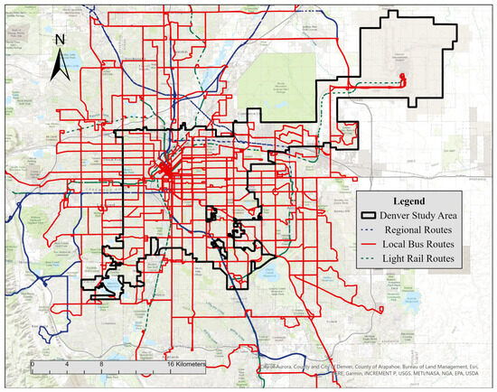
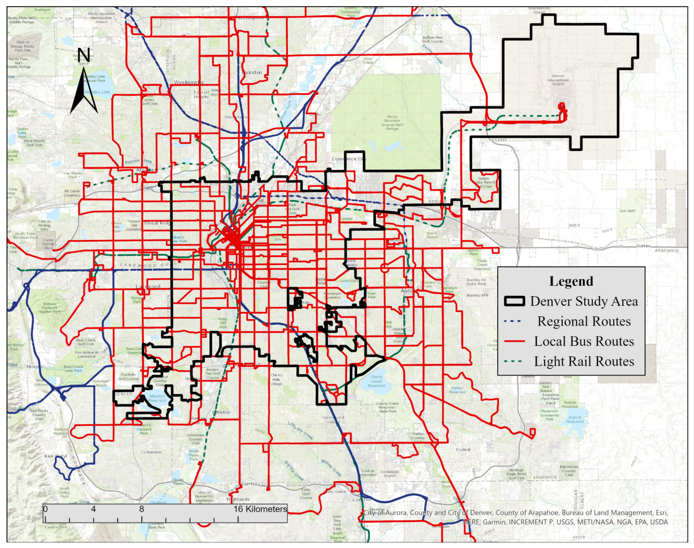
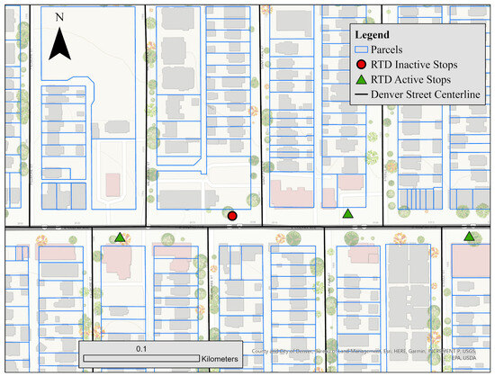
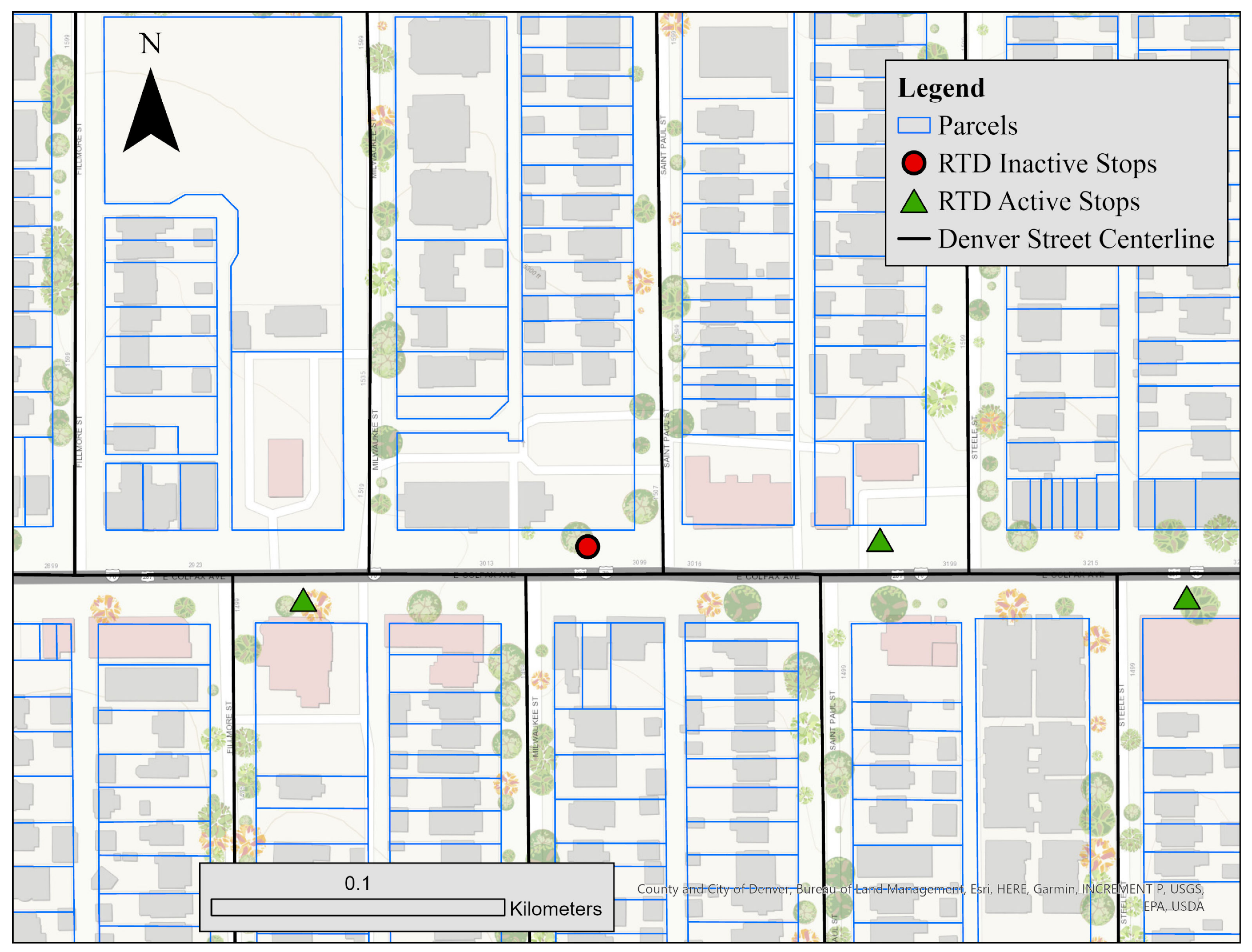
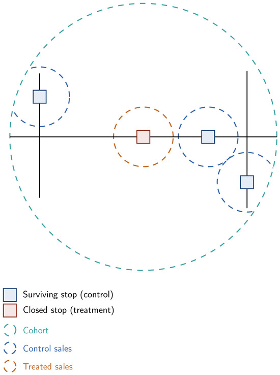
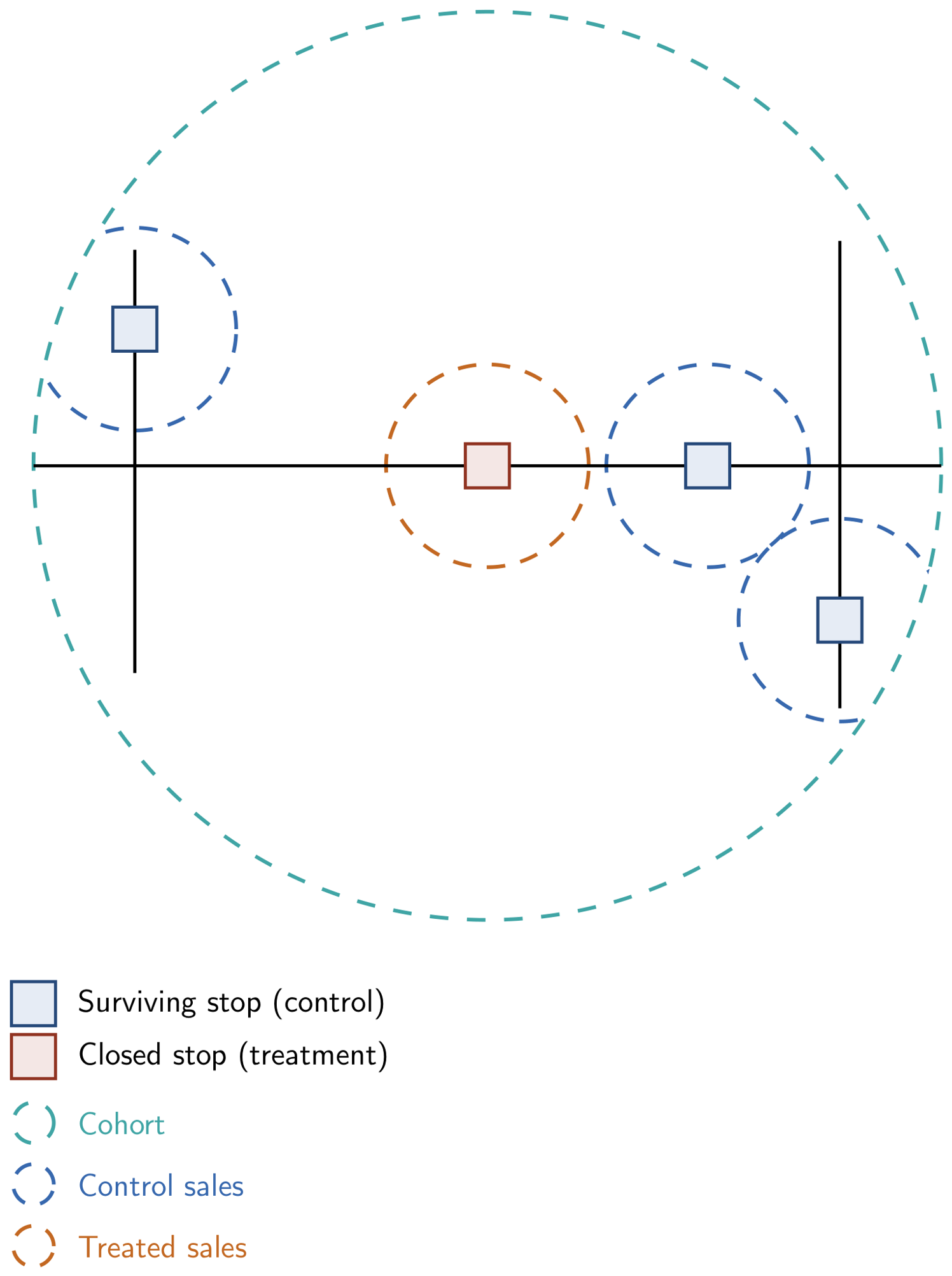
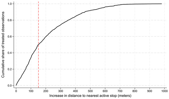
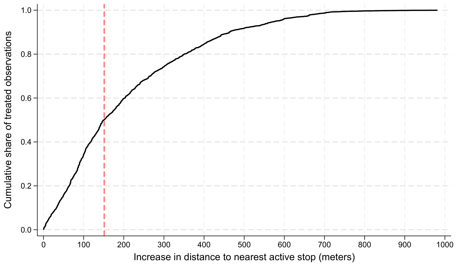
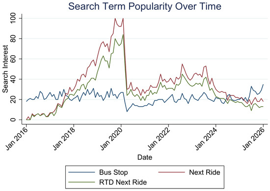
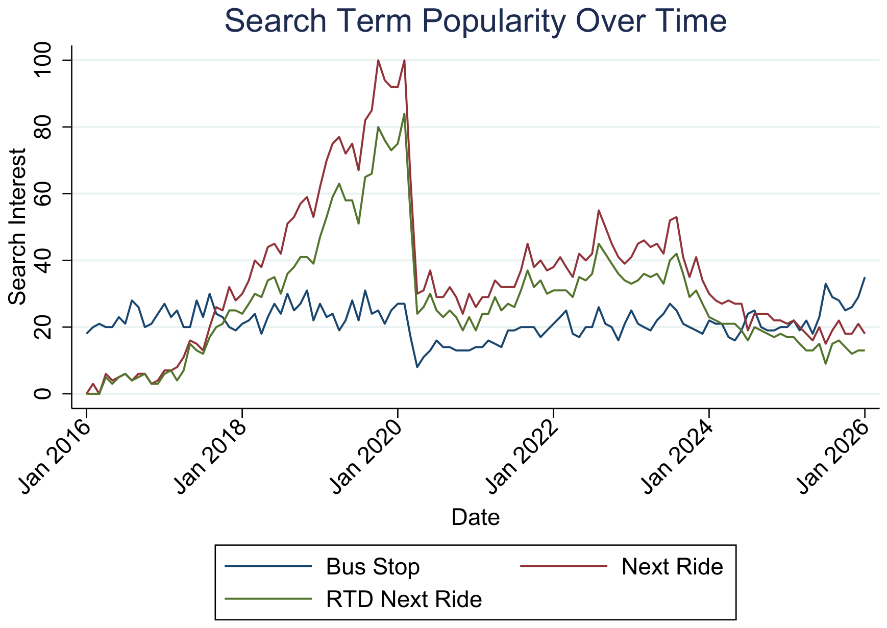
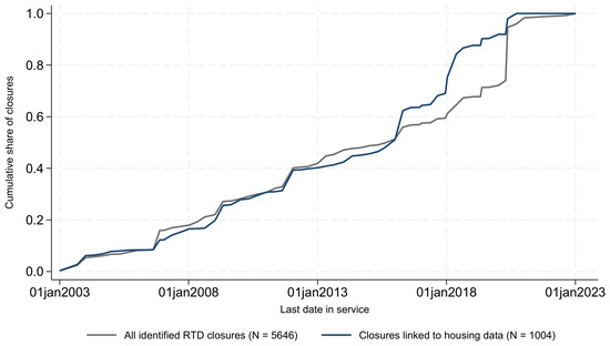
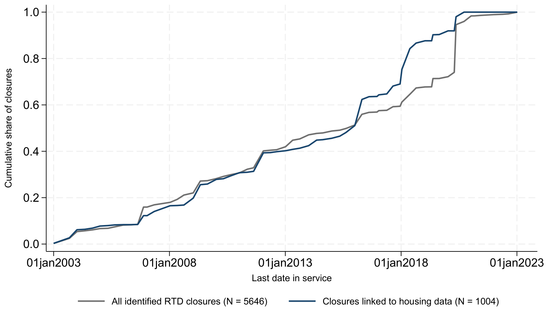
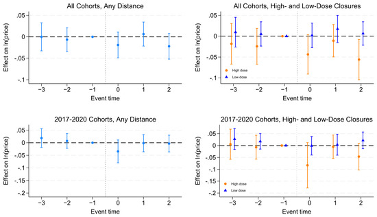
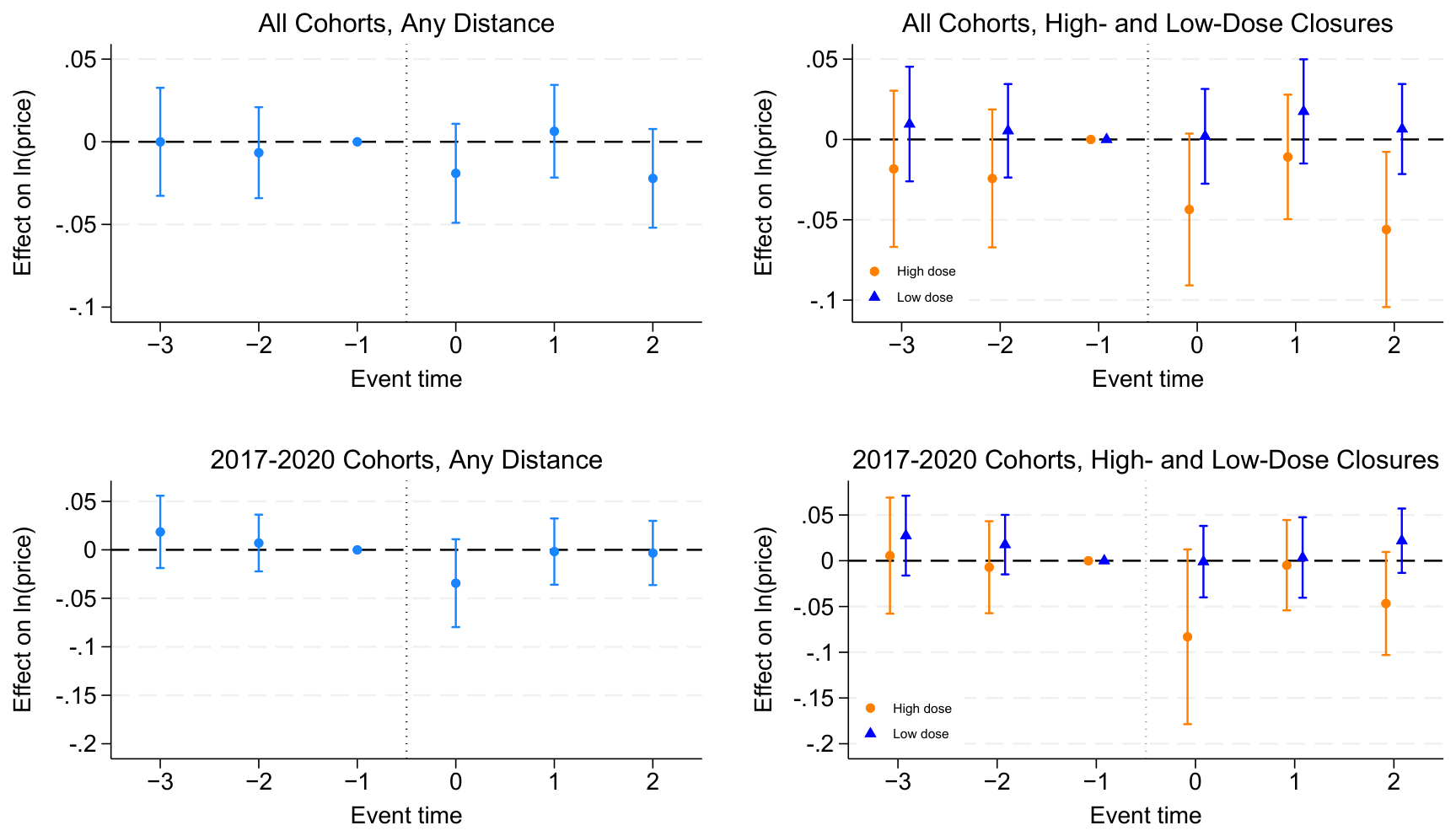
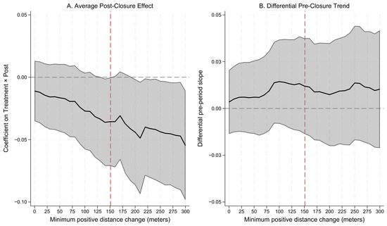
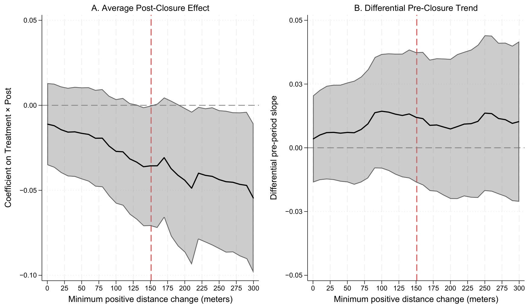
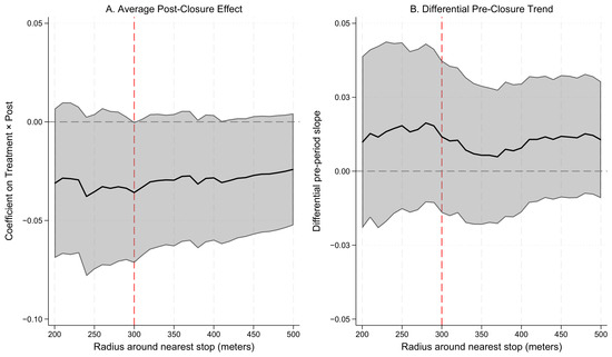
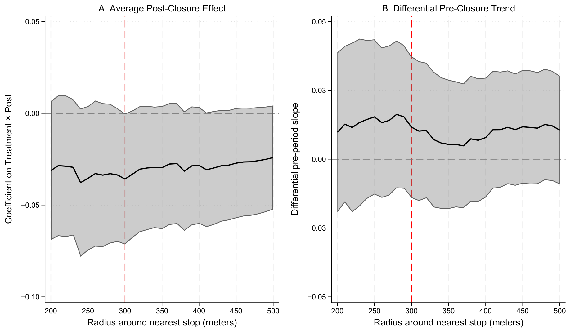
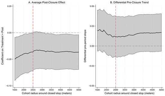
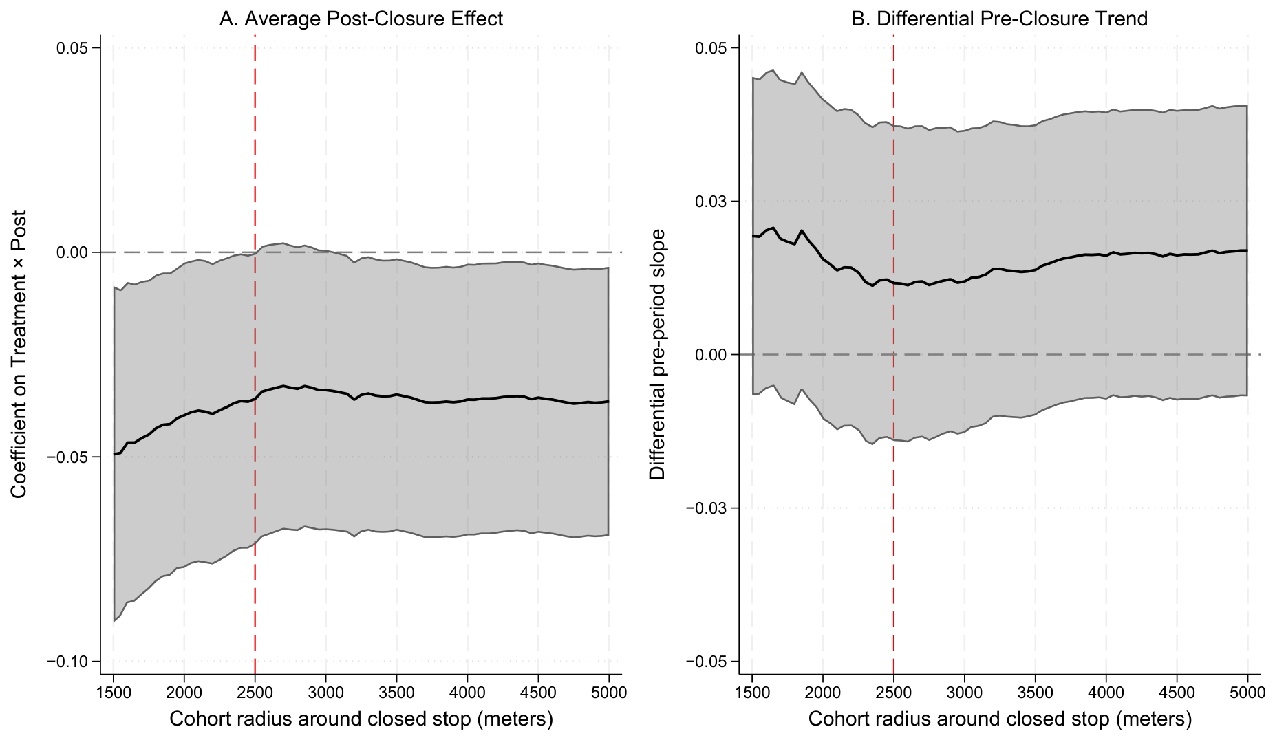

Disclaimer/Publisher’s Note: The statements, opinions and data contained in all publications are solely those of the individual author(s) and contributor(s) and not of MDPI and/or the editor(s). MDPI and/or the editor(s) disclaim responsibility for any injury to people or property resulting from any ideas, methods, instructions or products referred to in the content. |
© 2026 by the authors. Licensee MDPI, Basel, Switzerland. This article is an open access article distributed under the terms and conditions of the Creative Commons Attribution (CC BY) license.