


Abstract
This paper develops a two-dimensional fully Lagrangian meshless fluid–structure interaction solver by integrating the Moving Particle Semi-implicit (MPS) method with continuum mechanics to investigate the nonlinear interaction between waves and floating bodies. The stability and accuracy of the proposed model are validated through several benchmark cases. Furthermore, the solver is employed to analyze the dynamic response of a flat plate floating body in waves. The numerically generated waves exhibit a minimum error of approximately −0.5% and a period consistent with theoretical values, maintaining a smooth and continuous free surface. Due to the inherent limitations of the two-dimensional wave-floating body simulation, the Root Mean Square Error (RMSE) of the interaction results ranges from 5.4% to 15.2%. These findings indicate that the proposed method provides a valuable reference for the design and analysis of floating structures in ocean engineering.
1. Introduction
Ocean engineering structures operate in harsh marine environments, where the complex wave–structure interaction (WSI) poses significant technical challenges to structural safety and motion performance [1]. Accurately predicting these interactions constitutes a critical scientific problem in marine engineering. Given the limitations of physical model tests, such as high costs and scale effects, the numerical wave basin has become a vital tool for simulating wave propagation and structure responses. However, to ensure the reliability of WSI modeling, there is an urgent need for improved numerical approaches, among which the precise construction of the wave environment serves as a fundamental prerequisite [2].
According to its principle, the wave-making technology of numerical wave tanks can be roughly divided into two categories [3]: pure numerical wave-making technology and physical wave-making technology. In pure numerical wave-making technology, the most common methods include source function wave-making [4,5,6] and setting wave-making boundary [7,8,9]. The wave generated by pure numerical wave-making technology is generally of high accuracy, but there are also some problems, such as sensitivity to the source area location, poor wave propagation stability, and inconsistent water quality. The pure numerical wave-making technology lacks the corresponding physical model, which is not convenient for comparison with the test tank [3]. In contrast, the simulated physical wave-making technology has certain advantages. These problems are more likely to occur in waves, which are a type of highly nonlinear, large-deformation free surface flow problem.
In wave-related CFD simulations, the advantages of meshless methods over traditional meshed method [10,11,12,13,14,15] are mainly reflected in: the elimination of the need for pre-definement and continuous redrawing of the mesh; natural adaptability to severe deformation, breaking, and splashing of free surfaces; avoidance of difficulties such as mesh entanglement and free surface reconstruction; better topological adaptability when dealing with complex processes such as moving boundaries, multiphase interfaces, and wave breaking; and easier algorithm implementation to handle large deformation and multibody motion problems. Smoothed particle hydrodynamics (SPH) and the moving particle semi-implicit (MPS) method are two relatively common meshless methods.
SPH and MPS methods have made some achievements in numerical wave making and the interaction between waves and floating bodies. Gómez gesteira et al. [16] studied the wave motion in the case of waves on the ship’s deck by the SPH method, and found that the waves showed different behavior above and below the deck. Under extreme conditions, a jet would form at the rear of the deck after the waves. Zheng et al. [17] used the incompressible SPH method (ISPH) and improved the interpolation scheme to study the interaction between waves and structures with different shapes, and compared it with the test, which is in good agreement on the whole. Monaghan et al. [18] studied the propagation process of a solitary wave on the inclined plane through the SPH method, and simulated and accurately reproduced the test. Cleary et al. [19] studied the motion of complex marine structures in waves through the SPH method, and the research showed that the impact of waves on the structure would have a destructive impact on the integrity of the structure. Liang et al. [20] established a two-dimensional (2D) numerical wave flume within the Weakly Compressible Smoothed Particle Hydrodynamics (WCSPH) framework, constructing the δ-SPHC model via the introduction of a correction matrix to ensure second-order computational accuracy while effectively suppressing the breakdown of momentum conservation and energy dissipation.
MPS performs well in regular wave generation and floating body response, but it suffers from numerical dissipation and wave height prediction bias. Yang [21] conducted numerical simulation research on the generation of regular waves and the interaction between regular waves and floating bodies based on the MPS method. The shape of the wave surface maintained good stability, and no obvious numerical dissipation was found, but the numerical solution of wave height was slightly lower than that of the analytical formula, with a slight discrepancy. Zha et al. [22] used the MPS method to simulate the wave-floating body interaction model, verified the interaction between a circular floating body with a diameter of 400 mm and a thickness of 15 mm and regular waves, and analyzed the hydrodynamic response of the floating body under regular waves at different wavelengths and fixed wave heights. However, there are some errors in the regular wave period and amplitude.
To address the above issues, researchers have conducted extensive studies, making improvements in areas such as dimensional simplification, stability enhancement, and boundary modeling. Zhang et al. [23] established a two-dimensional numerical wave tank based on the improved MPS method and conducted numerical research on the free rolling motion of a two-dimensional floating body under the action of regular waves, including wave generation, wave absorption, and the motion of the floating body module. Renzi et al. [24] established a wave flume based on the Moving Particle Semi-implicit (MPS) method, featuring the implementation of a novel artificial viscosity scheme as its key characteristic. Lucas et al. [25] proposed a methodology employing an array of thin inclined slats as an alternative to conventional particle-based raster solid boundary modeling, establishing an MPS-based virtual gate (VG) model. Zhong et al. [26] developed a stabilized GPU-accelerated Moving Particle Semi-implicit (MPS) framework incorporating an internal correction matrix, and proposed a numerical wave flume model built upon this framework for the generation of high-precision waves.
The improvements to the MPS method are too numerous to cover here; the above only includes a portion. The improved MPS method offers enhanced accuracy and stability, and can be combined with other numerical methods to simulate complex fluid–structure interaction problems. Some progress has already been made in this area.
Zhang [27] established the heterogeneous beam equivalent model of a three-dimensional ship elastomer based on the MPS-FEM coupling solution strategy. The numerical simulation research on the coupling mechanism of the elastic hull and three-dimensional solitary wave load is carried out, which is further extended to the analysis of fluid–structure interaction in a regular wave environment, and the influence of elastic deformation of the elastic body on ship motion characteristics is included in the research. Zhang et al. [28] solved the hydroelasticity response of floating elastomers by using the MP method and the finite element method coupling calculation method, and simulated the impact of three-dimensional deformable floating platforms/ships in waves. Rao [29] established a numerical wave tank based on the fluid–structure interaction solver of the meshless method, and generated solitary waves by using the push plate, a physical wave-making method. From the results, the solitary wave peak in the numerical pool is very close to the theoretical value, and the waveform remains good in the process of propagation, and the wave height does not show obvious attenuation. Arash et al. [30] extended the parallel code via OpenMP to a three-dimensional potential numerical wave flume for fully nonlinear wave-body interactions.
These two methods have many similarities. Both are “particle methods” and both achieve the interaction between particles through kernel functions. The difference is that SPH uses the equation of state to solve the pressure based on the weak compressibility assumption, while MPS uses the pressure Poisson equation based on the incompressibility assumption. In wave problems, fluids are involved in the interaction with various types of boundary conditions. Therefore, whether the calculation model itself can accurately reflect the boundary conditions will directly affect the accuracy of the simulation. Since the MPS method uses the Poisson equation to implicitly solve the pressure field, it not only has a variety of means to accurately construct different types of boundary conditions, but also makes it possible for the pressure at various points in the flow field to respond to changes in boundary conditions instantaneously. From this perspective, the MPS method has certain advantages in wave problems [2].
To sum up, as a classic problem in ocean engineering, scholars have carried out a lot of research on the interaction between waves and floating bodies, but the traditional grid method based on physical wave-making technology is prone to grid distortion. To solve this problem, some scholars began to use the meshless method. At present, there have been some achievements in the study of the interaction between waves and floating bodies by using the MPs method, but the overall lack of comprehensive and detailed analysis and verification of the numerical pool, and the existence of tension instability and other problems, mean the free surface of the generated waves is not smooth.
Therefore, this paper establishes an MPS-FSI numerical flume solver, conducts comprehensive and in-depth verification and analysis, and, in conjunction with the work of previous scholars, introduces a hybrid source term, an optimized particle migration algorithm, a regularized gradient operator, and a stable operator model after extensive testing, in order to improve the problem of non-smooth free surfaces in the flow field.
2. Materials and Methods
In this study, the fluid and structure are controlled by different sets of governing equations. By introducing various models within the MPS framework and employing semi-implicit and explicit schemes, coupled models are established using different time steps and boundary conditions.
2.1. MPS Fluid Model
2.1.1. Governing Equations
In fluid mechanics, viscous incompressible flow satisfies the Navier–Stokes (N-S) equation and continuity equation:
where is the density; is time; is the velocity vector; is pressure; is kinematic viscosity; is gravity; is the gradient operator (Nabla Operator); is the Laplace operator (Laplacian); and is divergence, respectively.
2.1.2. Prediction Correction Algorithm
MPS uses an implicit format for pressure calculations, while the other term uses an explicit format, which is called “semi-implicit”. It is actually a prediction correction algorithm. Details are as follows [31]:
For the N-S equations, they can be expressed as follows:
The left-hand side of the equation can be decomposed as follows:
where superscript is the predicted (intermediate) vector; superscript represents the (k + 1)-th time step; is the k-th time step; and is the time step, respectively.
Comparing Equations (3) and (4) yields the following:
Based on Equation (5), the predicted velocity can be determined as follows:
Then, the predicted position is obtained from the predicted velocity:
where is the position vector.
At this point, performing a mathematical transformation on Equation (6), we first take the divergence of both sides:
For incompressible flow, the continuity equation is satisfied, i.e., (Equation (1)); thus, Equation (9) can be transformed into
Rearranging Equation (10) yields the following:
Equation (11) is the Poisson equation. By solving it, the pressure of each particle can be obtained. Then, combining Equations (6) and (11), the corrected velocity and corrected position of the particles can be determined as follows:
2.1.3. MPS Basis
In the MPS method, based on the idea of weighted average for particle approximation, the physical quantity of any particle is represented by the discrete sum of the physical quantities of other particles around it.
where is any vector and scalar (e.g., velocity, pressure) of the particle; is the kernel function (weighting function); and is the particle distance between, , respectively.
This article adopts the weighting function proposed in the original MPS method [31]:
where is the effective radius, in this study, = 2.1 times the initial particle distance (particle length, ), respectively.
In the prediction correction algorithm, the and need to be calculated. In the MPS method, the discretized models of these operators are expressed as [31]:
where is the spatial dimension; is the Laplacian correction coefficient; and represent particle number density and its initial value.
Based on Equations (1) and (11), combined with the MPS particle number density concept, the Poisson equation for the MPS method can be derived as follows:
where denotes the temporary particle number density corresponding to the predicted velocity and predicted position. The term on the right-hand side is referred to as the “source term”. Generally, the linear system of equations in Equation (20) can be solved using the Conjugate Gradient (CG) method.
2.1.4. MPS Supplementary Model
- (1)
- Neighborhood particle search algorithm
The MPS method approximates physical quantities through weighted averaging and computes the gradient and Laplace operators via discretized models. Consequently, it is necessary to search, index, and count the neighboring particles surrounding each particle.
Commonly, neighborhood particle search algorithms mainly include three types [32]: the all-pair search, the tree-based search, and the linked-list search. The all-pair search exhibits relatively low computational efficiency, particularly for cases with a large total number of particles. The tree-based search involves high complexity in implementation. Considering these factors comprehensively, the linked-list search is identified as the appropriate method. As shown in Figure 1, the specific implementation procedure is as follows:
Figure 1.
Schematic diagram of the linked-list search method.
(I) A background mesh (referred to as Cell) is constructed over the entire computational domain, with square cells of side length . It can be observed that each particle belongs to one and only one cell. The cell affiliation information for each particle is recorded accordingly.
(II) Each cell typically contains multiple particles; therefore, a linked list is established to record the particle index information contained within each cell.
(III) Evidently, the neighboring particles of the target particle i can only be located within the 9 cells surrounding the cell in which particle i resides.
(IV) Based on Step III, and according to the particle i → Cell → particle j information preserved in Steps I and II, the neighbors are accessed sequentially; subsequently, if , then particle j is identified as a neighboring particle.
- (2)
- Gradient operator with correction matrix
Using the original MPS method to calculate pressure gradient (Equation (16)), when the value is negative, it will cause attractive forces between particles, leading to non-physical aggregation of particles and ultimately accumulating errors, making the calculation unstable. To address this issue, this article adopts the gradient operator correction model proposed by Khayyer [32,33]:
where is the correction matrix, which is represented as follows:
where and is the horizontal and vertical coordinates of the particle, respectively.
- (3)
- Hybrid source terms
In the original MPS method, the source term (Equation (20)) is entirely composed of particle number density. For the problem of intense particle motion in the flow field, the particle number density field is inevitably not smooth, which leads to an unsmooth pressure field and can cause computational divergence in severe cases.
Considering these issues, Khayyer et al. [33], Tanaka et al. [34], and Zhang et al. [35] combined Equations (1) and (20) to obtain the mixed source term:
where is an artificially controlled parameter with a value range of [0, 1]. In this study, , respectively.
- (4)
- Particle shifting model
The discretization models of the original MPS method are all based on uniform particle distribution, and their accuracy cannot be guaranteed when the particle distribution in the flow field is chaotic [34,35]. Therefore, it is necessary to correct the particle positions upon the completion of each time step computation. This study adopts the Optimized Particle Shifting (OPS) algorithm proposed by Khayyer et al. [36]. Compared with the classical Particle Shifting (PS) algorithm, OPS permits position correction for free-surface particles only in the tangential direction, thereby avoiding the inaccuracy in displacement correction of free-surface particles encountered in the PS algorithm, as illustrated in Figure 2. In this study, , and times the initial particle distance.
Figure 2.
Schematic diagram of OPS [36].
- (5)
- Stabilization algorithm (STA)
The MPS method exhibits numerical instability, which may arise from the discontinuity and non-smoothness of the physical quantity fields.
Therefore, based on the work of Monaghan et al. [37], Ren et al. [38] assumed that the Laplacian operator values for different effective radii () are approximately equal and subtracted them. This approach preserves the stabilizing effect on the computation while alleviating the excessive non-physical numerical damping introduced by the original model. The specific details are as follows:
where the superscripts and denote the states after and before the correct, respectively. Both and are artificially controlled parameters with a value range of [0, 1], employed to adjust the intensity of the STA. is derived from the Laplace operator in the finite difference method.
In this study, the STA procedure is applied to the fluid particle velocities () subsequent to the OPS treatment. and ; and , respectively.
2.2. MPS Structure Model
This article is based on the finite deformation analysis theory of continuum mechanics combined with the MPS method to establish a numerical model of a structure model.
2.2.1. Continuum Mechanics
The basic assumptions and formula derivation of the theory of finite deformation analysis have been provided in a large number of studies, and will not be elaborated on in this article. Please refer to the works of Javier [39] and Reddy [40] for details.
The control equation of nonlinear elastic dynamics, namely the momentum equation of elastic bodies in the Hamiltonian framework, is derived through the variational principle and the principle of minimum action. It is described as follows:
where is particle acceleration; the superscripts S and F denote the structure and the fluid, respectively; is the strain energy density function; and is the acceleration applied by adjacent fluid particles on the target elastic particle.
where is the divergence of with respect to the initial coordinate system; the superscript 0 represents the initial position of the structural particle. is the second Piola–Kirchhoff tensor; Symbol “:” denotes the double dot product; is the identity matrix; is the deformation gradient tensor; is the first Piola–Kirchhoff tensor; and are Lame’s constants; is the Young’s modulus; is the Poisson’s ratio; is trace; is the green strain tensor; is the initial configuration position information; and is the current configuration position information.
The relationship between and is known as the constitutive relationship of the material. In this study, the Saint Venant–Kirchhoff model is adopted.
2.2.2. MPS Discretization Continuum Mechanics (MPS-CM)
This section presents the discretized model (operators) based on the MPS method for computing continuum mechanics, as described below:
(1) Calculate deformation gradient tensor
Substituting Equations (16), (21), (22) into Equation (32) yields the discretized formulation for computing :
where denotes the position vector.
(2) Green strain tensor , the first Piola–Kirchhoff tensor , the second Piola–Kirchhoff tensor
At this stage, is known. Then, according to Equations (28)–(33), , , can be calculated sequentially (→→).
(3) Divergence
Considering the relatively small number of particles on the structural surface, a conservative gradient model is introduced to ensure computational stability [41]:
By combining Equation (34) with Equations (16), (21), (22), the value of can be obtained as follows:
Then, the double dot product of and can be computed.
(4) Particle acceleration
By substituting Equation (14) into Equation (13), the acceleration of the structural particles can be obtained.
On the right-hand side of the equation, is known. Further details regarding will be provided in the subsequent section on boundary conditions.
(5) Update the particle velocity and position.
where denotes the computational time step for structural particles, which is generally much smaller than that for the fluid; in this study, a ratio of 1:1000 is maintained.
(6) STA
After each structural time step is calculated, STA is applied to the velocity and position of structural particles to eliminate unreasonable numerical oscillations.
2.3. Boundary Condition
2.3.1. Free-Surface Boundary
Once a fluid particle is identified as a free-surface particle, its pressure is forcibly set to zero. As shown in Figure 3, one side of a free-surface particle lacks neighboring particles, resulting in a lower particle number density compared to that of interior fluid particles. This characteristic can be used to identify free-surface particles:
Figure 3.
Schematic diagram of free surface and wall boundary conditions.
If the above criterion is satisfied, the particle is identified as a free-surface fluid particle; this means it does not participate in the pressure solution, and the pressure is directly assigned a value of zero.
2.3.2. Wall Boundary Condition
In the MPS method, to ensure the integrity of the particle influence domain, the object surface is typically arranged with one layer of first-type wall boundary particles and two layers of second-type wall boundary particles (as shown in Figure 3). This multi-layered arrangement avoids particle penetration and influence domain truncation, ensuring the integrity of the influence domain at the object surface.
The pressure of the first-type wall boundary particles is solved using the Poisson equation and is consistent with that of the fluid particles; the pressure of the second-type wall boundary particles is obtained by interpolation of the surrounding fluid particles and the first-type wall boundary particles. When the wall is stationary, the velocities of both types of boundary particles are set to zero; when the wall is moving, their velocities are determined according to the motion characteristics of the object.
2.3.3. Fluid–Structure Interface Condition
- (1)
- The effect of the structure on the fluid.
When computing the fluid area, the structure is treated as a wall boundary.
- (2)
- The effect of the fluid on the structure.
When computing the structural area, the fluid provides external forces that drive the motion and deformation of the structure.
As shown in Figure 4, the force exerted by fluid particles on structural particles acts only on their contact interface. Therefore, when computing the direction and magnitude of the force on the structure, only particles within the effective radius of the fluid particles are considered. The details are as follows:
Figure 4.
Methods for calculating the direction and magnitude of the force exerted by a fluid on a structure.
To determine the direction of the force, we perform calculations on the relevant structural surface particles:
where represent the direction of the applied force. To obtain the magnitude of the force exerted by the fluid on the solid:
In the fluid computation, the pressure acting on the structural particles has already been obtained. The magnitude of the external force can then be calculated as the product of the pressure and the area over which it acts. Clearly:
where the superscripts and denote the fluid and the structure, respectively. is the force exerted by fluid particles on structural particles; is the pressure of the structural particles (already computed in the fluid domain); is the area over which the force acts on the structural particles; is the mass of the structural particles; and is the volume of the structural particles, respectively.
2.4. Fluid–Structure Interaction (FSI)
In this study, the fluid and structural models are constructed using different governing equations and different time-stepping schemes, while sharing the same MPS discretization framework (mainly the gradient and Laplacian operators). The advantage of this approach is that the fluid and structural models can operate independently or be coupled through boundary conditions.
As shown in Figure 5, the detailed computational procedure is as follows:
Figure 5.
Flowchart of the FSI computation procedure.
2.5. Parallel Computing
This article uses the Compute Unified Device Architecture (CUDA) programming model and writes computational code based on the C/C++ language. As shown in Figure 6, the Central Processing Unit (CPU) is mainly used for initialization, controlling kernel function execution, visualization, etc. The computing work is entirely executed by the Graphics Processing Unit (GPU), and all the data required for the computation is stored on the GPU. The GPU used in this study is the NVIDIA Tesla A100 80 GB PCIe.
Figure 6.
GPU parallel strategy.
We used the CG method to iteratively solve the pressure Poisson equation. The pressure iterations for each particle were calculated in parallel using GPU kernel functions. For the part requiring the calculation of the global dot product, to ensure reproducible numerical errors and facilitate program development, we implemented global accumulation using reduction instead of CUDA’s atomic addition function (AtomicAdd). Most parts of the code can be parallelized well, but two parts reduce computational efficiency: one is the convergence residual used to determine iteration termination in the CG method. Due to the low efficiency of dynamic parallel computation in CUDA, this residual must be sent back to the host to determine whether the iteration has terminated, making it difficult to use streaming acceleration here. The other is the penalty calculation for the sparse matrix. Because the topological relationships of the spatial positions between particles in the meshless method change over time, memory alignment is difficult for the GPU when accessing video memory, which also reduces access efficiency to some extent.
3. Results
This study develops a coupled numerical model for wave–flexible slender floating structures by integrating a Moving Particle-Semi-implicit (MPS) fluid solver with a finite-deformation solid solver.
First, the fluid scheme, the solid scheme, and their coupling are verified independently through three benchmark cases: hydrostatic pressure in a tank, free vibration of a cantilever beam, and an elastic plate under hydrostatic load. Next, a numerical wave flume is then established; its accuracy is confirmed by comparing the present results with analytical solutions, published numerical data, and experimental measurements, thereby laying a solid foundation for the subsequent coupled simulations. Finally, having demonstrated the reliability of the overall numerical framework, parametric investigations are conducted to elucidate the dynamic behavior of flexible floating bodies under various wave conditions.
3.1. Model Validation
3.1.1. Fluid Model Validation
Figure 7a presents the schematic of the hydrostatic-pressure benchmark adopted herein. The working fluid is water = 1000 kg/m3, under standard gravity = 9.81 m/s2 with a kinematic viscosity of = 10−6 m2/s. A pressure probe is positioned at the geometric center of the tank bottom to record the temporal evolution of the hydrostatic pressure. Figure 7b summarizes the grid-convergence study for the numerical solution of pressure against analytical solutions. As the length of the particle () is progressively refined, the predicted pressure monotonically converges to the theoretical value. When = 0.0025 m, the relative error,
is only 0.5%, demonstrating the accuracy and robustness of the present Lagrangian solver.
Figure 7.
Model schematic diagram: (a) graph of pressure variation over time at detection points; (b) the grid-convergence study.
3.1.2. Solid Model Validation
To verify the accuracy of the proposed solid model, the free vibration of a cantilever beam subjected to an initial force is investigated [42]. The cantilever specimen considered herein is 48.0 m in length and 12.0 m in height, with its left end fully clamped and a concentrated downward force applied at the free right tip. The load is instantaneously removed at = 0.5 s. The material is characterized by a Young’s modulus of = 3.0 × 10⁷ Pa, a Poisson’s ratio of = 0.3, and a mass density of = 1.0 kg/m3; plane-stress conditions are assumed throughout, and no artificial numerical damping is introduced. During the forced excitation phase (0–0.5 s), the cantilever beam depicted in Figure 8 executes strictly periodic vertical oscillations; the instantaneous tip displacement remains bounded above by the undeformed reference level, exhibiting no overshoot. After load release ( ≥ 0.5 s), the structure performs free vibrations that are strictly periodic and virtually symmetric with respect to the geometric mid-axis.
Figure 8.
Schematic diagram of the free vibration model of a cantilever beam with a given initial force.
Figure 9 presents the transient vertical displacement of the cantilever tip as a function of time. The computed response is in excellent agreement with theoretical expectations. Progressive refinement of the particle spacing reveals that both amplitude and period rapidly approach the reference finite-element solution; the numerical predictions converge monotonically with high fidelity. These results demonstrate that the adopted elastic solid model accurately captures dynamic, impulsive loading scenarios.
Figure 9.
The numerical simulation results of the cantilever beam displacement in this paper are compared with those of FEM [42]: (a) overall image; (b) detail of time history.
3.1.3. FSI Model Validation
The stability and accuracy of the fluid–structure interaction scheme are assessed through a classical benchmark involving a hydrostatic water column resting on an elastic plate. Originally introduced by Fourey et al. [42], the configuration is depicted in Figure 10a. The water column is 2.0 m in height and 1.0 m in length. The water column = 2.0 m and = 1.0 m, with = 1000 kg/m3, = 9.81 m/s2, and = 10−6 m2/s. At = 0 s, the column is gently deposited on an initially undeformed aluminum plate that is clamped at both ends; hence, the hydrostatic pressure is applied quasi-instantaneously rather than gradually. The aluminum plate is 0.05 m thick and spans the same length as the water column; its material properties are = 2700 kg/m3, = 67.5 GPa and = 0.34. The benchmark focuses on the temporal evolution of the plate’s mid-span displacement, thereby emphasizing the sensitivity of the coupling strategy to high-frequency hydrodynamic loading.
Figure 10.
(a) Schematic of the model structure; (b) steady-state pressure field and elastic-plate stress distribution predicted by the model.
Figure 10b presents the hydrostatic pressure field in the fluid and the corresponding Cauchy stress field in the elastic plate at = 10.0 s, as predicted by the present solid-mechanics solver. At this instant, the high-frequency eigenmodes of the water column and the aluminum plate have fully decayed, and the coupled system has reached a stationary equilibrium. The stress state in the base plate exhibits near-perfect symmetry about the mid-plane, in excellent agreement with the reference solution of Fourey et al. [42].
Figure 11 summarizes the convergence study for the elastic plate subjected to hydrostatic pressure, computed with the present solid-mechanics solver. Four discrete resolutions are examined, corresponding to particles across the aluminum plate thickness. The associated minimum stable time steps are = 10−4 s for the fluid and = 10−7 s for the solid. The abscissa denotes time, while the ordinate records the mid-span deflection of the plate. As the simulation proceeds, the predicted deflections for all resolutions collapse onto a single equilibrium value, and the discrepancy between successive refinements diminishes monotonically, attesting to the convergence of the present scheme. Concurrently, the duration of high-frequency transients increases with decreasing particle size, a direct consequence of the reduced numerical damping inherent to the stabilizing operator.
Figure 11.
Convergence test results of elastic plates under hydrostatic pressure reproduced by the structural numerical model in this article.
To quantify the accuracy of the present scheme, Table 1 summarizes the relative errors in the predicted mid-span deflection of the elastic plate under hydrostatic pressure. The proposed solid solver yields a relative error of 2.8%, demonstrating that the elastic model and the fluid–structure interaction strategy adopted herein are both accurate and reliable.
Table 1.
Displacement of deflection at the center point of the elastic plate.
3.2. Numerical Wave Tank
Guided by the rigorous validation detailed in the preceding section, a numerical wave tank is developed in this study. Wave generation is implemented via an idealized piston-type wavemaker, while a numerical sponge layer is positioned downstream to effectively mitigate spurious reflections. Regular waves spanning a broad parametric range of wave numbers are systematically generated, with the resulting free-surface elevations rigorously benchmarked against analytical solutions. These comprehensive assessments establish a robust, validated foundation for all subsequent investigations.
The equation of motion for the wave-making plate follows the formulation proposed by Dean [43]:
In this equation, denotes the displacement of the paddle, and represents the paddle velocity. signifies the wave height, while represents the wavenumber derived from the dispersion relation. denotes the wave frequency, represents the wave period, and signifies the time variable. refers to the stroke amplitude of the paddle, and is the still water depth. Finally, and correspond to the hyperbolic sine and cosine functions, respectively.
The wave-damping equation follows the formulation established by Zhang et al. [44], with the damping effect applied to the fluid velocity within the designated damping zone at the conclusion of each time step:
In this equation, and denote the velocity after and before damping correction, respectively. represents the damping factor, while indicates the particle position. signifies the length of the damping zone, and marks the starting position of the zone. and are coefficients governing the damping intensity, typically assigned values of 0.1 and 6.0. Finally, denotes the exponential function.
To quantify wave attenuation, the wave reflection characteristics of the flume—commonly referred to as “reflectivity”—must be determined. The classical two-point method proposed by Goda [45] is employed, whereby two wave gauges are positioned along the wave propagation direction to synchronously record surface elevations. Fourier series decomposition is subsequently utilized to separate the incident and reflected wave components, from which the reflection coefficient is calculated. To prevent numerical singularities, the spacing between the gauges must be distinct from any integer multiple of half the wavelength.
Ren et al. [46] experimentally investigated the temporal evolution of the dynamic response of a free-floating body within the wave flume at Dalian University of Technology and validated the associated numerical model. The geometric parameters of the current numerical wave tank are directly adopted from this physical study, as illustrated in Figure 12. Waves are generated by a piston-type wavemaker at the left boundary, while a numerical damping zone on the right boundary prevents wave reflection by adjusting the flow field velocity. Four wave gauges (No. 1–No. 4) are installed in the central region at 0.5 m intervals. The target wave height is = 0.04 m with a period of = 1.2 s. The gravitational acceleration is set to = 9.81 m/s2, the kinematic viscosity to = 10−6 m2/s, and the maximum Courant number is maintained at 0.1.
Figure 12.
Schematic diagram of the numerical wave tank model.
3.2.1. Convergence Test
Figure 13 compares the free-surface elevations obtained using different initial particle lengths under the conditions specified in Table 2 (still-water depth = 0.4 m, wave period = 1.2 s, target wave height = 0.04 m). A slight fluctuation is observed during the initial stages of the simulation. The free surface subsequently settles into a steady oscillation state within approximately 15 s, and the resulting period aligns with the target value. The measured wave heights demonstrate monotonic convergence as the particle size decreases. These findings confirm that the numerical wave tank is both stable and reliable, exhibiting no significant numerical dissipation.
Figure 13.
Convergence test results of spatial: (a) overall image; (b) detail of time history.
Table 2.
Some quantitative indicators of convergence test results.
Table 2 presents a quantitative evaluation of the stability and accuracy of the wave generation model using several metrics, including spectral analysis (Fast Fourier Transform, FFT), mean wave period, and mean wavelength. The analysis is conducted based on the results of ten wave cycles from the case with the smallest particle spacing shown in Figure 13. The results indicate that the numerical predictions are in excellent agreement with the theoretical values in terms of both wave period and wave height, with relative differences well below 1%. As illustrated in Figure 14, the wave spectrum exhibits two distinct peaks, among which the dominant peak is significantly larger than the secondary one. This characteristic is consistent with the typical spectral features of regular waves. To balance accuracy and computational cost, a particle spacing of = 0.0015 m is selected.
Figure 14.
Spectral analysis of waves.
3.2.2. Damping Parameter Test
If the coefficient and (Equation (49)) within the damping layer are set too low, incident waves penetrate the layer and reflect off the downstream end wall. Conversely, an excessive factor causes the incident waves to reflect from the damping region itself, thereby generating spurious reflections. Consequently, an optimal coefficient and must be determined.
The reflectivity and wave amplitude obtained using various damping parameters are summarized in Table 3 and Table 4. Initially, decreasing reduces the reflection coefficient, which reaches a minimum at = 0.0025. However, a further reduction in reverses this trend and amplifies the reflections. An analogous behavior is observed for : the reflection coefficient decreases as is reduced, but rebounds once a critical threshold is surpassed. The wave amplitude exhibits a similar pattern; the amplitude error diminishes as reflectivity decreases and increases when reflectivity rises again. Consequently, properly tuned damping parameters effectively suppress spurious reflections, confirming the physical consistency of the model. Based on the data in Table 3 and Table 4, the damping coefficients = 0.0025 and = 3.0 are selected for all subsequent simulations.
Table 3.
Reflectance test for ca.
Table 4.
Reflectance test for na.
Figure 15 presents the temporal evolution of surface elevation recorded at each wave gauge after adjusting the parameters based on analyses of particle length convergence and damping parameter sensitivity. The flow field continues to develop during the initial 15 s, evidenced by transient oscillations in the surface elevation traces at all wave gauges. After = 15 s, the flow attains a statistically steady state, and the recorded wave amplitudes stabilize into consistent oscillations. The results demonstrate that the wave period and amplitude are spatially uniform across all gauges and show satisfactory agreement with the analytical solution.
Figure 15.
The wave height time history of each wave height detection point, with lp = 0.0015 m, ca = 0.0025, and na = 3.0: (a) overall image; (b) detail of time history.
Figure 16 presents an instantaneous snapshot of the global pressure field and the local particle arrangement = 15 s, obtained from the current simulation. Examination of the particle distribution adjacent to the free surface reveals a smooth interface free of spurious numerical ripples. This observation further corroborates the accuracy and numerical stability of the proposed numerical wave tank.
Figure 16.
Overall distribution of flow field pressure and local particle distribution (t = 15 s, lp = 0.0015 m, ca = 0.0025, na = 3.0).
3.2.3. Validation of Regular Waves with Varying Dimensionless Water Depth
To assess the applicability and accuracy of the current MPS-based numerical wave tank, a systematic series of regular waves with varying parameters is investigated. Table 5 summarizes the test matrix, in which the dimensionless water depth is varied according to Equation (26) from Yun [47], whereas the target wave height H and still-water depth h remain fixed at 0.04 m and 0.40 m, respectively. The sponge layer configuration and all other numerical wave tank parameters are consistent with those previously described.
Table 5.
Regular waves with different dimensionless depths.
Figure 17 presents a comparison of the calculated wave height-to-paddle stroke ratio () with reference to numerical data and analytical predictions, indicating a close agreement. Compared with the SPH-based computations of Yun [47], the present MPS solutions exhibit superior fidelity to the theoretical curve. Collectively, these findings demonstrate that the proposed MPS numerical wave tank robustly and accurately reproduces regular waves across a range of parameters. In conclusion, the MPS numerical wave tank developed in this study generates stable and accurate regular waves throughout the entire parameter range examined.
Figure 17.
Comparison of transfer function with linear theory (the SPH result is from Yun [47]).
3.3. Interaction of Waves with a Rigid Floating Box
To evaluate the stability of the MPS-based numerical wave tank model presented in this study and its feasibility for wave–rigid floating body interaction problems, this section establishes a numerical model based on the physical experiments of Ren [46] and investigates the motion response of a floating body under regular wave action. A schematic of the numerical wave tank is shown in Figure 18. Initially, a square, rigid, floating box is positioned in the tank, 4.6 m from the wave maker. The box has a height of 0.2 m, a length of 0.3 m, a density of 500 kg/m3, and a mass of 30 kg.
Figure 18.
Schematic diagram of the interaction model between waves and rigid floating bodies.
Figure 19 visually illustrates the motion of the floating body and the evolution of the free surface over one cycle. The results demonstrate that the numerical simulations presented in this study are in excellent agreement with the experimental data regarding the motion of the floating body and the wavefront morphology.
Figure 19.
Comparison of floating body motion and free surface in one cycle (t = t0 + 0.25/0.5/0.75/1.0T): (a1–a4) the present work result; (b1–b4) Ren’s experiment result [46].
Figure 20 illustrates the time history of a floating body’s motion in regular waves. The horizontal axis is normalized by the wave period, the vertical axis by the wave height, and the deflection angle by the relative water depth. As shown in the figure, the floating body is subjected to wave impact in the horizontal direction; its motion exhibits a continuously rising, stepped sinusoidal pattern, manifested as lateral drift rather than merely moving reciprocally with the fluid. A comparison with the experimental results of Ren [46] indicates that the numerical values in this study show better agreement with the experimental data than those obtained via the SPH method. In the vertical direction, the floating body heaves with the wave surface. Regarding angular motion, the floating body rotates with changes in the free surface, and the deflection angle is symmetric about the equilibrium position. The results in this paper are basically consistent with the experimental results.
Figure 20.
Time history curve of floating box motion under regular wave action (experiment result and SPH result are from Ren et al. [46]): (a) surge; (b) heave; (c) deflection angle.
To quantitatively compare the numerical results with the experimental results, Table 6 presents the root-mean-square error (RMSE) and phase difference calculated based on the results in Figure 19. The calculation formula is as follows:
Table 6.
Quantitative comparison of numerical results and experimental results interaction of waves with a rigid floating box.
Here, is the number of samples, specifically the number of data points within the 0–5 s interval; is the corresponding vertical coordinate value; the superscripts and denote the numerical results and experimental results, respectively; is the time delay, which in this case is the difference in the average period between the numerical results and the experimental results; and is the average period of the experimental results.
It can be observed that in terms of horizontal motion (X/h), MPS shows significantly lower RMSE, time difference, and phase difference compared to SPH, indicating higher numerical accuracy and better phase consistency. In terms of vertical motion (Y/h), MPS achieves a notably lower RMSE, demonstrating more accurate amplitude simulation, while SPH performs slightly better in time synchronization and phase difference, showing a somewhat stronger phase retention capability. Regarding angular motion (θ/kh), SPH outperforms MPS across all three error metrics, with a particularly pronounced advantage in phase difference. Overall, MPS has greater advantages in simulating horizontal motion and vertical amplitude, whereas SPH performs slightly worse in capturing the temporal characteristics of vertical phase and angular motion.
In summary, the numerical results presented in this study are in good agreement with the experimental data. This indicates that the developed MPS numerical wave tank possesses good stability, verifying its feasibility and accuracy in simulating wave–rigid body interaction problems.
3.4. The Problem of Wave-Float Interaction
The motion of floating bodies in waves exhibits highly nonlinear characteristics. Floating bodies act as boundary conditions for waves and cause wave reflections near the floating body, affecting the shape of the waves. Waves exert wave forces on floating bodies, causing changes in their position and shape, further altering the boundary conditions of the waves.
These two interactions are coupled with each other and inevitably exhibit highly nonlinear characteristics. This brings uncertainty and difficulties to the research. Therefore, it is necessary to conduct in-depth research on the motion of floating bodies in waves under different floating body and wave parameter conditions.
3.4.1. Verification
McGovern, D.J., and Bai, W [48] conducted model experiments on the motion of floating bodies in regular waves. In their experiment, paraffin was used as the float with a density of 890 kg/m3, a length of 0.3 m, a height of 0.05 m, an elastic modulus of 2.0 GPa, and a Poisson’s ratio of 0.3, and it was assumed that paraffin was isotropic. In this example, considering that the experimental focus of the model is on the motion law of the stable state of the floating body in the rules and the calculation time of the numerical coupling model constructed in this paper, a numerical testing model, as shown in Figure 21, is constructed. Place the floating body model 3 m away from the wave-making plate, and set the left wave-making plate motion according to wavelength = 3.0 m, wave height = 0.148, and static water depth = 0.9 m. The other settings of the numerical sink are the same as before.
Figure 21.
Schematic diagram of the floating body motion model in regular waves.
Figure 22 shows the comparison between the numerical results of floating body motion in this paper and the experimental results of McGovern, D.J., and Bai, W [48]. The figure shows the result of the floating body reaching a stable motion state. It can be seen that although there are inevitable differences due to different dimensions, the numerical results of the MPS method in this paper are relatively consistent with the experimental values in the longitudinal and vertical oscillation directions. This provides some support for proving that the MPS wave elastic floating body coupling numerical model established in this paper can predict the behavior of floating bodies in waves and obtain accurate numerical results.
Figure 22.
Comparison between numerical results of the floating body model motion and experimental results [48]: (a) surge; (b) heave.
Table 7 provides a quantitative analysis of the numerical and experimental results. RMSE and phase difference were calculated using Equations (50) and (51), and AEXP denotes the average peak-to-peak amplitude. It can be seen that the numerical method used can generally reproduce the observed motion response well, but there are differences in simulation accuracy across different degrees of freedom. In the horizontal direction (X), the numerical results and experimental curves show good consistency in amplitude and phase, with small RMSE and phase differences.
Table 7.
Quantitative comparison of numerical results and experimental results of wave-float interaction verification.
In Figure 22a, the peaks and troughs of the two curves are basically aligned, indicating that the model has high reliability in predicting horizontal motion. In the vertical direction (Y), the error between the numerical results and experimental curves is relatively significant, with both RMSE and phase differences greater than in the horizontal direction. In Figure 22b, some deviations can be observed in the local extreme value positions and waveform morphology, reflecting that the model’s accuracy in simulating vertical motion still needs improvement. This difference may be related to the accuracy of wave field reconstruction, structural dynamic response model parameters, and the simulation of damping effects.
3.4.2. The Problem of Wave-Float Interaction with Different Float Length
Using the method of controlling variables, study the effect of parameter changes on the motion of a floating body while keeping other physical parameters unchanged and changing a single parameter. The changing parameters include float length, float thickness, wavelength, and wave height. The commonly used parameters to describe the motion behavior of floating bodies include: floating body motion period, average amplitude of longitudinal and vertical displacement, maximum stress applied, and maximum deflection angle. In this article, these parameters are taken from the data of the floating body in a stable motion state for 6 cycles.
As shown in Table 8, keeping the height, wavelength, and wave height of the floating body unchanged, changing the length of the floating body with a spacing of 0.15 m, gradually increasing from 0.15 m to 0.75 m. The maximum ratio of the length of the floating body to the length of the wave reaches 0.25.
Table 8.
Floating body model parameters of different lengths.
Table 9 shows the Response Amplitude Operator (RAO) of floating bodies with different lengths in waves. Overall, as the length of the floating body continues to increase, the movement period of the floating body does not change significantly. The motion period of the floating body in Case 1–Case 3 is basically the same. At this time, the length of the floating body is very small compared to the wavelength, so the influence of the floating body on wave motion is relatively slight, and it continues to move with almost the same period as the waves. As the length ratio of the floating body increases, the reflection of waves by the floating body is enhanced, further interfering with the flow field. Causing a slight slowdown in the motion cycle of the floating body. It can be foreseen that as the length of the floating body further increases, its motion cycle will further slow down, which is consistent with the real physical situation. Under wave excitation, the Response Amplitude Operator (RAO) of floating bodies exhibits significant variations across different motion modes with changes in scale. For a surge, where the hydrostatic restoring force is negligible, the response is primarily governed by the balance between wave excitation, inertia, and damping. As the length of the floating body increases, the expansion of the wave-facing area significantly enhances the excitation force; meanwhile, the contribution of the inertia term remains limited under low-frequency conditions. Consequently, the surge RAO increases with body length. In contrast, for heave, the restoring force is proportional to the waterplane area and increases substantially with length, while the growth in added mass amplifies the inertial effects. Furthermore, when the body length approaches the wavelength, partial cancellation of the wave excitation occurs due to phase differences. As a result of these combined factors, the heave RAO decreases with increasing floating body length.
Table 9.
RAO of floating bodies with different lengths.
As illustrated in Figure 23, the numerical results reveal significant wave run-up on the floating structure. This phenomenon influences the body dynamics through two distinct mechanisms: first, the entrapment of run-up water on the deck increases the effective mass of the floater (equivalent to increased density), creating a positive feedback loop that exacerbates the wave run-up tendency; second, the slamming impact generated by the run-up water substantially alters the motion response of the structure. Furthermore, owing to the two-dimensional nature of the present numerical model, the run-up water cannot freely drain laterally from the deck, resulting in continuous mass accumulation and introducing systematic numerical errors. The study indicates that wave run-up intensity increases monotonically with floater length; when the length exceeds a critical threshold, the combined effects of the aforementioned positive feedback mechanism and accumulated numerical errors lead to significant distortion in the motion response. Wave run-up phenomena have also been reported in the study by McGovern, D.J., and Bai, W [48].
Figure 23.
Comparative analysis of length effects on wave run-up behavior of floating bodies (case 1 to case 5, from left to right).
Figure 24a,b visually illustrate various states of wave-float interaction with different float lengths. It can be seen that at the same time, the longer the length of the floating body, the greater its longitudinal displacement value, and the growth gradient law is not obvious, with almost the same motion period. On the contrary, as the length of the floating body increases, its heave displacement value decreases. Table 9 quantitatively describes this phenomenon through the motion Response Amplitude Operator. The Response Amplitude Operator (RAO) is an important parameter that describes the motion response characteristics of a floating body in waves. It is defined as the ratio of the motion amplitude of the corresponding degrees of freedom of the floating body to the wave amplitude, indicating the motion response characteristics of the floating body under linear wave action. The RAO (longitudinal oscillation) and RAO (vertical oscillation) in this article refer to the average amplitude of the floating body motion over the six cycles shown in Figure 24b.
Figure 24.
Various states of wave-float interaction with different float lengths: (a) the longitudinal oscillation displacement diagram; (b) the vertical oscillation displacement diagram; (c) the variation in float deflection angle; (d) maximum stress under different lengths of float conditions.
Figure 24c shows the curve of the deflection angle of floating bodies of different lengths in waves over time. From the figure, it can be seen that the deflection angle of floating bodies in waves exhibits obvious periodicity, and the deflection periods of floating bodies of different lengths are almost equal. In terms of amplitude, when a floating body moves in waves, its deflection angle is negatively correlated with its length. At the same time, it can be observed that as the length of the floating body increases, its deflection angle curve gradually becomes smoother. In case 1, the length of the floating body is relatively short, and its deflection angle curve has a slight twist. As the length of the floating body changes, this phenomenon disappears, and the deflection curve of the floating body tends to be smooth. This phenomenon is attributed to the influence of the fluid in the run-up region on the motion of the floating body. As the total mass of the floating body increases with its length, the relative contribution of this effect diminishes to a negligible level. Further investigation is required to elucidate this phenomenon.
Figure 24d shows the maximum stress (the normal stress component in the x-direction) diagram of floating bodies of different lengths moving in waves. The stress distribution of a floating body in waves generally varies periodically with its motion state. Here, the average of the maximum stress values experienced by the floating body during its six cycles of motion in waves is taken as the maximum stress experienced by the floating body. It can be seen that as the length ratio of the floating body to the wave increases, the maximum stress on the floating body increases exponentially with the length of the floating body.
3.4.3. The Problem of Wave-Float Interaction with Different Wave Length
This section adopts a similar method, keeping the length of the floating body at 0.3 m and the height at 0.05 m unchanged, and changing the wave height and wavelength values in the wave parameters to study the influence of wave parameter changes on the results. The wave parameters are shown in Table 10. The motion behavior of the floating body model in different wave parameters is analyzed using the floating body motion period, average amplitude of longitudinal and vertical displacement, maximum stress, maximum deflection angle, and floating body wave reflectivity.
Table 10.
Study on the influence of waves of different wavelengths on floating body motion.
Figure 25a,b illustrate the time-history curves of the floating body’s motion under various wavelength conditions. Qualitatively, the period of each curve increases correspondingly with the wavelength. As the wavelength increases, the wave period lengthens; consequently, within the fixed time interval of 12–21 s, the floating body undergoes fewer oscillation cycles, decreasing from six cycles in Case 6 to five in Case 9. Furthermore, the longitudinal oscillation amplitude of the floating body gradually decreases with increasing wavelength, whereas the variation in vertical oscillation amplitude is relatively minor.
Figure 25.
Various states of wave-float interaction with different wavelengths: (a) the longitudinal oscillation displacement diagram; (b) the vertical oscillation displacement diagram; (c) the variation in float deflection angle; (d) maximum stress under different lengths of float conditions.
Table 11 quantitatively presents the motion response operators of the floating body for different wavelength conditions. Analysis of the tabulated data reveals that the trend in the floating body’s motion period is consistent with the variation in wavelength. While the longitudinal oscillation amplitude gradually decreases with increasing wavelength, the vertical oscillation amplitude exhibits a slight increase, though the overall magnitude of variation remains small. Under wave excitation, the response characteristics of the floating body exhibit distinct features as the wavelength varies. Specifically, for surge, the excitation primarily stems from the horizontal gradient of wave pressure. As the wavelength increases, the wave slope diminishes, resulting in a significant reduction in the horizontal pressure gradient. This attenuation weakens the excitation force, thereby causing a gradual decrease in the surge response amplitude. In contrast, heave is primarily governed by the overall vertical displacement of the wave field; its excitation is more directly correlated with the wave amplitude and is consequently less sensitive to variations in wavelength. Furthermore, given the dominance of hydrostatic restoring forces and inertial effects, the heave response amplitude exhibits minimal variation with changing wavelength.
Table 11.
RAO of floating body motion under different wavelength conditions.
Figure 25c presents the variation curves of the floating body’s angular deflection under different wavelength conditions. The results indicate that the maximum angular deflection of the floating body decreases progressively as the wavelength increases. When other parameters remain constant, increasing the wavelength leads to a reduction in wave steepness, rendering the wave profile gentler; consequently, the decrease in angular deflection is physically consistent. Further analysis based on wave theory reveals that wavelength serves as the critical parameter governing the geometric morphology of waves and the distribution characteristics of hydrodynamic loading. As the wavelength increases, the diminishing wave steepness causes the waveform to approach a flatter profile, a transition that results in reduced pressure gradients within the flow field and consequently yields a more uniform distribution of vertical excitation forces along the floating body’s length. Therefore, the differential lift forces induced by wave undulations and the corresponding induced bending moments are significantly attenuated. Such spatially gentler wave loading effectively suppresses the rigid-body rotational response of the floating structure, thereby diminishing the maximum angular deflection. Simultaneously, the combined effects of reduced load concentration and diminished structural deformation amplitude lead to a continuous decrease in maximum internal stresses, elucidating the physical mechanism underlying the attenuation of hydrodynamic excitation under long-wave conditions.
Figure 25d shows the maximum stress curve of the floating body under different wavelength conditions. The horizontal axis in the figure represents the ratio of the length of the floating body to the wavelength. Since the length of the floating body remains constant, a larger value indicates a smaller wavelength. Therefore, the horizontal axis from left to right is case 9–case 6. From the graph, it can be seen that as the wavelength increases, the maximum stress on the floating body decreases continuously, as in Table 11.
Overall, as the wavelength increases, the length ratio decreases accordingly. Therefore, the overall effect of increasing wavelength on the motion behavior of floating bodies in waves is similar to reducing the length of floating bodies. However, due to the strong nonlinear nature of the interaction between waves and floating bodies, the changes in the amplitude of floating body motion and wave reflectivity are not completely consistent with changing the length of the floating body.
3.4.4. The Problem of Wave-Float Interaction with Different Wave Heights
This section adopts the same method to explore the variation in floating body motion response under different wave height conditions. In the test, parameters such as float scale, wavelength, and pool settings were kept constant, and the value of wave height was changed to observe the impact of wave height changes on the results. The parameter settings are shown in Table 12.
Table 12.
Parameter table for studying the influence of waves with different wave heights on the motion of floating bodies.
Figure 26a,b show the duration curves of heave and heave of a floating body under different wave heights. The influence of wave height on the oscillation and heave periods is relatively small, and there are only slight differences in the resulting period values for different wave heights, with little overall variation. In terms of amplitude, the amplitude of the heave and the heave of the floating body are positively correlated with the height of the wave.
Figure 26.
Various states of wave-float interaction with different wave heights: (a) the longitudinal oscillation displacement diagram; (b) the vertical oscillation displacement diagram; (c) the variation in float deflection angle; (d) maximum stress under different lengths of float conditions.
Table 13 quantitatively describes this change. Overall, the period of the floating body changes very little, while the amplitude increases with the increase in wave height, and this increase shows a linear increasing trend. This change is reasonable because, as the wave height increases, the wave energy becomes higher and more concentrated, and the amplitude of the floating body’s motion changes more significantly. Therefore, it can be foreseen that the rotation angle and maximum stress of the floating body also increase with the increase in wave height. The results in Figure 26c confirm this, and the horizontal axis in Figure 26d represents the wave height value. Under varying wave heights, both the surge and heave Response Amplitude Operators (RAOs) of the floating body increase with wave height, exhibiting an approximately linear relationship; notably, the heave RAO is generally larger than the surge RAO. This phenomenon is attributed to the fact that increasing wave height enhances wave energy, thereby amplifying the wave excitation force. Since the mass and restoring force of the floating body remain substantially constant, the response amplitude increases approximately linearly with the excitation. Furthermore, heave motion is more strongly governed by hydrostatic restoring forces, rendering it more sensitive to variations in wave energy, whereas surge, lacking such restoring force constraints, exhibits a relatively slower rate of growth.
Table 13.
RAO of floating body motion under different wave height conditions.
In summary, the influence of wave height on the interaction between waves and floating bodies is quite significant in all aspects. Overall, as wave height increases, the amplitude, deflection angle, and maximum stress of the floating body’s motion also increase. The variation in the floating body’s motion period is not significant, while the reflectivity of floating body waves shows the opposite.
4. Discussion
The present parametric investigation provides comprehensive insights into the dynamic response characteristics of flexible floating structures under varying geometric configurations and wave conditions. The numerical results demonstrate distinct response patterns across the investigated parameter space.
With respect to the length-scale effects, as the floater length increases from 0.15 m to 0.75 m, the response period remains virtually invariant at small length-to-wavelength ratios (L/λ < 0.15), exhibiting synchronization with the incident wave period; however, upon exceeding a critical threshold, wave reflection intensifies considerably, inducing a slight elongation of the motion cycle. The surge amplitude exhibits a monotonic increasing trend with the length ratio, whereas the heave amplitude demonstrates an inverse relationship, thereby reflecting the combined influence of enhanced floater inertia and amplified horizontal excitation forces.
Of particular significance is the wave run-up phenomenon, which intensifies monotonically with floater length and influences the hydrodynamic loading through two distinct mechanisms: (i) the entrapment of run-up water on the deck increases the effective mass, thereby establishing a positive feedback loop that exacerbates the run-up tendency; and (ii) the slamming impact generated by the overturning water substantially alters the structural motion response characteristics.
Regarding the wavelength-dependent response, the results exhibit qualitatively analogous yet quantitatively distinct characteristics compared to the length-scale effects. As the wavelength increases from 2.5 m to 4.0 m, the wave period extends correspondingly, resulting in a reduction in oscillation cycles within the fixed observational window. The surge amplitude gradually attenuates with increasing wavelength, whereas the heave amplitude exhibits a modest increasing trend, consistent with the physical mechanism whereby increasing wavelength reduces wave steepness.
Concerning the influence of wave height, numerical simulations indicate that wave height exerts a relatively minor influence on the floater motion period, which aligns with the predictions of linear wave theory. However, both surge and heave Response Amplitude Operators (RAOs) exhibit an approximately linear increasing trend with increasing wave height. Notably, the heave RAO is consistently larger than the surge RAO across the investigated range. The underlying physical mechanism for this behavior is that increasing wave height enhances wave energy, thereby augmenting the wave excitation force; given that the mass and restoring force of the floating body remain substantially unchanged, the response amplitude grows approximately linearly with the excitation. Furthermore, the distinction in RAO magnitudes can be attributed to the differing roles of restoring forces: heave motion is governed by strong hydrostatic restoring forces, rendering it more sensitive to variations in wave energy, whereas surge motion lacks such restoring force constraints, resulting in a relatively slower rate of increase.
Overall, the motion response characteristics obtained from the present numerical simulations demonstrate strong consistency with theoretical expectations: increasing floater length leads to enhanced inertia and amplified horizontal excitation forces, thereby resulting in increased surge amplitudes; conversely, increasing wave height directly augments the wave energy input, leading to linear growth in response amplitudes with distinct sensitivities due to restoring force disparities. The observed wave run-up phenomenon, which occurs due to the comparable densities between the floating body and water, further complicates the hydrodynamic interaction. However, it should be noted that the wave-floating body interaction problem exhibits highly nonlinear characteristics, particularly due to the existence of wave run-up and slamming effects, which render complete theoretical prediction challenging and underscore the significance of the present numerical investigation.
The two-dimensional modeling framework, while computationally efficient, cannot account for the lateral outflow of deck run-up water, thereby preventing the dissipation of accumulated mass to the sides as would occur in three-dimensional configurations. This limitation results in progressive mass accumulation on the deck and potential systematic biases in the predicted motion response characteristics.
Despite the achievements of this study, certain limitations remain that warrant consideration in future investigations. First, the model is currently limited to a two-dimensional framework and cannot fully capture the complex three-dimensional flow fields and wake effects around actual marine structures such as ships and offshore platforms. Secondly, the Saint Venant–Kirchhoff constitutive model adopted herein is suitable for large deformation and small strain conditions; however, this model cannot simulate potential plastic deformation or more complex nonlinear material behaviors. Furthermore, in cases involving long floating bodies, the wave run-up phenomenon observed on the deck may be overestimated due to the inability to account for lateral outflow effects, potentially leading to systematic biases in the calculation results. Additionally, the meshless particle-based programming methodology, while offering distinct advantages for free-surface flows, involves constantly evolving particle positions that preclude aligned memory access as achievable in conventional meshed methods, thereby limiting computational efficiency. Future research should focus on extending the present framework to three-dimensional configurations, incorporating more sophisticated material models capable of capturing plastic deformation, and implementing advanced computational strategies to enhance numerical efficiency.
5. Conclusions
In this study, a two-dimensional fully Lagrangian meshless fluid–structure interaction solver was established by integrating the Moving Particle Semi-implicit (MPS) method with continuum mechanics. The numerical framework was comprehensively validated through systematic benchmark cases. First, the fluid model was verified against the analytical solution for hydrostatic pressure in a tank, achieving a relative error of merely 0.5% with refined particle spacing. Second, the solid model was validated through the free vibration of a cantilever beam under impulsive loading, demonstrating excellent agreement with theoretical and finite element solutions in terms of oscillation amplitude and period. Third, the fluid–structure interaction scheme was assessed using an elastic plate under hydrostatic pressure. Here, the predicted mid-span deflection converged to a relative error of 2.8% upon mesh refinement, and the steady-state pressure and stress fields were free from spurious oscillations. Subsequently, a numerical wave tank was established featuring piston-type wave generation and a sponge layer damping zone. Convergence studies confirmed that a particle spacing of 0.0015 m offers an optimal balance between accuracy and computational cost. Lastly, the wave tank was validated against experimental measurements of rigid floating body motions, showing superior agreement compared to existing SPH results.
Based on the above validation, parametric investigations on flexible floating bodies revealed distinct response patterns under varying geometric and wave conditions. Increasing the floater length while maintaining constant wave parameters amplified the surge amplitude and maximum stress, whereas the heave amplitude and maximum deflection angle decreased monotonically. The motion period remained essentially unchanged at small length-to-wavelength ratios but exhibited slight elongation as structural interference with the wave field intensified. Notably, pronounced wave run-up on the deck was observed with increasing floater length, introducing additional mass effects and slamming impacts. Variations in wavelength produced effects qualitatively similar to inverse variations in floater length; however, the strong nonlinearities inherent in wave–structure interactions resulted in quantitatively distinct response patterns for wave reflectivity and motion amplitudes. Increasing wave height induced linear growth in both surge and heave amplitudes, along with significant increases in the maximum deflection angle and stress, while the motion period remained insensitive to wave height variations.
Overall, the developed model successfully captured smooth free-surface evolution and stable pressure fields without numerical instability, providing a new option for subsequent research on nonlinear wave–structure interactions.
Author Contributions
Conceptualization, X.F., D.R., J.S.P., X.H., J.S. and K.C.; Methodology, X.F., D.R. and J.S.P.; Software, X.F. and D.R.; Validation, X.F.; Formal analysis, X.F. and D.R.; Investigation, X.F., D.R. and J.S.; Resources, D.R., J.S.P., X.H. and Z.M.; Data curation, X.F. and J.S.; Writing—original draft, X.F.; Writing—review and editing, X.F., D.R., J.S.P., X.H. and K.C.; Visualization, X.F.; Supervision, D.R., J.S.P., X.H. and Z.M.; Project administration, D.R.; Funding acquisition, D.R., X.H. and Z.M. All authors have read and agreed to the published version of the manuscript.
Funding
This research was funded by the Natural Science Foundation of Guangxi, grant number AD23026005; the Major Science and Technology Projects of Guangxi, grant numbers AA24206015 and AA22068105; the Key Research and Development Program of Guangxi, grant number AB25069083; the middle-aged and young teachers’ basic ability promotion project of Guangxi Zhuang Autonomous Region of China, grant number 2023KY0440.
Data Availability Statement
The original contributions presented in this study are included in the article. Further inquiries can be directed to the corresponding author.
Acknowledgments
The authors acknowledge the use of GLM (version 4.7, https://chatglm.cn/, accessed on 10 February 2026) for language editing purposes, specifically for grammatical verification and paragraph-level polishing. The AI tools were employed solely to improve readability and linguistic accuracy. All scientific content, data interpretation, and conclusions remain the sole responsibility of the authors.
Conflicts of Interest
The authors declare no conflicts of interest.
References
- Li, H.J.; Liu, F.S.; Du, J.F. Development Trend and Technical Challenges of Ocean Engineering. Coast. Eng. 2022, 41, 283–300. [Google Scholar]
- Hitoshi, G.; Abbas, K. Current achievements and future perspectives for projection-based particle methods with applications in ocean engineering. J. Ocean. Eng. Mar. Energy 2016, 2, 251–278. [Google Scholar]
- Li, H.W. The Research of Wave-Generating Method in Numerical Tank. Master’s Thesis, Harbin Engineering University, Harbin, China, 2009. [Google Scholar]
- Brorsen, M.; Larsen, J. Source Generation of nonlinear gravity waves with boundary integral equation method. Coast. Eng. 1987, 11, 93–113. [Google Scholar] [CrossRef] [Scilit]
- Ohyama, T.; Nadaoka, K. Development of a numerical wave tank for analysis of nonlinear and Irregular wave field. Fluid Dyn. Res. 1991, 8, 231–251. [Google Scholar] [CrossRef] [Scilit]
- Chen, Y.; Hsiao, S. Generation of 3D water waves using mass source wavemaker applied to Navier-Stokes model. Coast. Eng. 2016, 109, 76–95. [Google Scholar] [CrossRef] [Scilit]
- Wei, G.; Kirby, J.T. Time-Dependent Numerical Code for Extended Boussinesq Equations. J. Waterw. Port Coast. Ocean Eng. 1995, 121, 251–261. [Google Scholar] [CrossRef] [Scilit]
- Jacobsen, N.G.; Fuhrman, D.R.; Fredsøe, J. A wave generation toolbox for the open-source CFD library: OpenFOAM. Int. J. Numer. Methods Fluids 2012, 70, 1073–1088. [Google Scholar] [CrossRef] [Scilit]
- Wang, D.; Dong, S. Generating shallow-and intermediate-water waves using a lineshaped mass source wavemaker. Ocean Eng. 2021, 220, 108493. [Google Scholar] [CrossRef] [Scilit]
- Zha, J.J. Numerical Model of Wave Generation and Absorption Based on OpenFOAM and Its Applications. Master’s Thesis, Shanghai Jiao Tong University, Shanghai, China, 2011. [Google Scholar]
- Liu, X. Numerical Simulation of Piston-Type Active Absorption Wave Making Based on OpenFOAM. Master’s Thesis, Tianjin University, Tianjin, China, 2022. [Google Scholar]
- Chen, Y. The Numerical Simulation of The Motion of Float in The Numerical Wave Tank. Master’s Thesis, Huazhong University of Science & Technology, Wuhan, China, 2020. [Google Scholar]
- Fei, Y.T. Research and Design of Rocker Panel Wave Generator System. Master’s Thesis, Huazhong University of Science & Technology, Wuhan, China, 2015. [Google Scholar]
- Yu, Y.F. Numerical Simulation of Wave and Analysis of Its Flow Field Structure. Ph.D. Thesis, Harbin Institute of Technology, Harbin, China, 2013. [Google Scholar]
- Zhu, Z.Y. Development and Application of a Coupled Wave-Flow Numerical Flume Based on the Mass Source Method. Ph.D. Thesis, East China Normal University, Shanghai, China, 2024. [Google Scholar]
- Gómez, G.M.; Cerqueiro, D.; Crespo, C. Green Water Overtopping Analyzed with a SPH Model. Ocean Eng. 2005, 32, 223–238. [Google Scholar] [CrossRef] [Scilit]
- Zheng, X.; Lv, X.; Ma, Q. An Improved Solid Boundary Treatment for Wave-Float Interactions Using ISPH Method. Int. J. Nav. Archit. Ocean Eng. 2018, 10, 329–347. [Google Scholar] [CrossRef] [Scilit]
- Monaghan, J.J.; Kos, A. Solitary Waves on a Cretan Beach. J. Waterw. Port Coast. Ocean Eng. 1999, 125, 145–155. [Google Scholar] [CrossRef] [Scilit]
- Cleary, P.W.; Rudman, M. Extreme Wave Interaction with a Floating Oil Rig: Prediction Using SPH. Prog. Comput. Fluid Dyn. 2009, 9, 332. [Google Scholar] [CrossRef] [Scilit]
- Liang, G.Q.; Yang, X.; Zhang, Z.F. Study on the propagation of regular water waves in a numerical wave flume with the δ-SPHC model. Appl. Ocean Res. 2023, 135, 103559. [Google Scholar] [CrossRef] [Scilit]
- Yang, B.Y. Research on Prediction Method and Influence Law of Ice Resistance of Ship in Broken Ice Conditions. Ph.D. Thesis, Dalian University of Technology, Dalian, China, 2022. [Google Scholar]
- Zha, R.S.; Zhao, W.W.; Wan, D.C. Numerical study of wave-ice floe interactions and overwash by a meshfree particle method. Ocean Eng. 2023, 286, 115681. [Google Scholar] [CrossRef] [Scilit]
- Zhang, Y.L.; Wan, D.C. Numerical study of interactions between waves and free rolling body by IMPS method. Comput. Fluids 2017, 155, 124–133. [Google Scholar] [CrossRef] [Scilit]
- Renzi, E.; Dias, F. Application of a Moving Particle Semi-Implicit Numerical Wave Flume (MPS-NWF) to model design waves. Coast. Eng. 2022, 172, 104066. [Google Scholar] [CrossRef] [Scilit]
- Lucas, S.P.; Rubens, A.A.J.; Cheng, L.Y. A numerical modeling of wave-inclined slats interaction for particle methods. Ocean Eng. 2024, 296, 116699. [Google Scholar] [CrossRef] [Scilit]
- Zhong, Y.P.; Sun, X.F.; Soares, C.G. Application of a correction matrix moving particle semi-implicit GPU solver on numerical wave flumes. Ocean Eng. 2025, 332, 121346. [Google Scholar] [CrossRef] [Scilit]
- Zhang, G.Y. Investigations and Applications of 3D MPS/FEM Coupled Method in Wave-Elastic Structure Interaction Problems. Ph.D. Thesis, Shanghai Jiao Tong University, Shanghai, China, 2022. [Google Scholar]
- Zhang, G.Y.; Zhao, W.W.; Wan, D.C. Moving Particle Semi-implicit method coupled with Finite Element Method for hydroelastic responses of floating structures in waves. Eur. J. Mech.-B/Fluids 2022, 95, 63–82. [Google Scholar] [CrossRef] [Scilit]
- Rao, C.P. Numerical study of the wave-induced slamming force on the elastic plate based on MPS-FEM coupled method. J. Hydrodyn. 2018, 30, 70–78. [Google Scholar] [CrossRef] [Scilit]
- Arash, A.; Soares, C.G. OpenMP parallelism in computations of three-dimensional potential numerical wave tank for fully nonlinear simulation of wave-body interaction using NURBS. Eng. Anal. Bound. Elem. 2020, 117, 321–331. [Google Scholar]
- Koshizuka, S.; Oka, Y. Moving-particle semi-implicit method for fragmentation of incompressible fluid. Nucl. Sci. Eng. 1996, 123, 421–434. [Google Scholar] [CrossRef] [Scilit]
- Wu, Q.R.; Wang, H.M. A Meshless Method—The Semi-Implicit Moving Particle Method MPS, 1st ed.; Shanghai Jiao Tong University Press: Shanghai, China, 2018; pp. 82–204. [Google Scholar]
- Khayyer, A.; Gotoh, H. Enhancement of stability and accuracy of the moving particle semi-implicit method. J. Comput. Phys. 2011, 230, 3093–3118. [Google Scholar] [CrossRef] [Scilit]
- Tanaka, M.; Masunage, T. Stabilization and smoothing of pressure in MPS method. J. Comput. Phys. 2010, 229, 4279–4290. [Google Scholar] [CrossRef] [Scilit]
- Zhang, S.; Lou, Y.M.; Xing, F. A new consistent particle interaction models for moving particle semi-implicit method. Chin. J. Comput. Mech. 2013, 30, 124–129. [Google Scholar]
- Abbas, K.; Hitoshi, G.; Yuma, S. Comparative Study on Accuracy and Conservation Properties of Two Particle Regularization Schemes and Proposal of an Optimized Particle Shifting Scheme in ISPH Context. J. Comput. Phys. 2017, 332, 236–256. [Google Scholar] [CrossRef] [Scilit]
- Monaghan, J.J. On the problem of penetration in particle methods. J. Comput. Phys. 1989, 82, 1–15. [Google Scholar] [CrossRef] [Scilit]
- Ren, D.; Park, J.C. Particle-based numerical simulation of continuous ice-breaking process by an icebreaker. Ocean Eng. 2023, 270, 113478. [Google Scholar] [CrossRef] [Scilit]
- Javier, B.; Richard, D.W. Nonlinear Continuum Mechainics for Finite Element Analysis, 2nd ed.; Cambridge University Press: Cambridge, UK, 1997; pp. 25–300. [Google Scholar]
- Reddy, J.N. An Introduction to Continuum Mechanics, 2nd ed.; Cambridge University Press: Cambridge, UK, 2008; pp. 20–225. [Google Scholar]
- Toyota, E.; Akimoto, H.; Kubo, S. A particle method with variable spatial resolution for incompressible flows. In Proceedings of the 19th Symposium on Computational Fluid Dynamics, Barga, Italy, 19–24 June 2005. [Google Scholar]
- Fourey, G.; Hermange, C.; Le, T.D. An efficient FSI coupling strategy between Smoothed Particle Hydrodynamics and Finite Element methods. Comput. Phys. Commun. 2017, 217, 66–81. [Google Scholar] [CrossRef] [Scilit]
- Dean, R.G.; Dalrmple, R.A. Wavemaker theory. In Water Wave Mechanics for Engineers and Scientists, 3rd ed.; World Scienfitic: Singapore, 1991; pp. 178–185. [Google Scholar]
- Zhang, N.; Zheng, X.; Ma, Q. Study on wave-induced kinematic responses and flexures of ice floe by Smoothed Particle Hydrodynamics. Comput. Fluids 2019, 189, 46–59. [Google Scholar] [CrossRef] [Scilit]
- Yoshimi, G.; Yasumasa, S. Estimation of Incident and Reflected Waves in Random Wave Experiments. Coast. Eng. 1976, 169, 49–50. [Google Scholar]
- Ren, B.; He, M.; Dong, P. Nonlinear Simulations of Wave-Induced Motions of a Freely Floating Body Using WCSPH method. Appl. Ocean Res. 2015, 50, 1–12. [Google Scholar] [CrossRef] [Scilit]
- Yun, S.M. Development of Fluid-Multibody Dynamics Coupling Simulation Method for Analysis of Power Generation Performance of Floating Wave Energy Converter in Waves. Ph.D. Thesis, Pusan National University, Busan, Republic of Korea, 2021. [Google Scholar]
- McGovern, D.J.; Bai, W. Experimental study on kinematics of sea ice floes in regular waves. Cold Reg. Sci. Technol. 2014, 103, 15–30. [Google Scholar] [CrossRef] [Scilit]
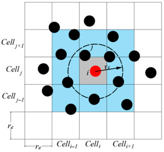
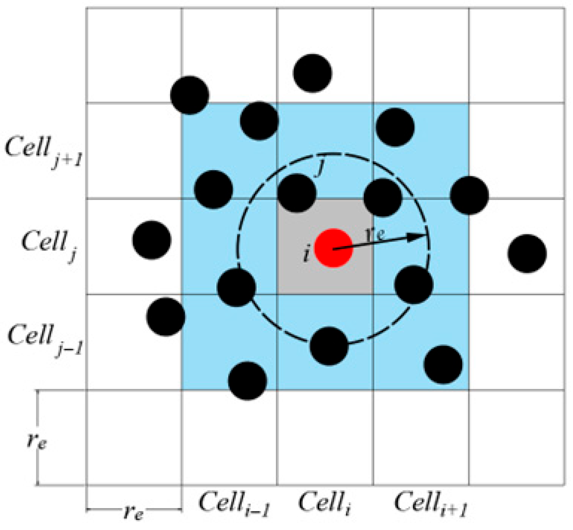
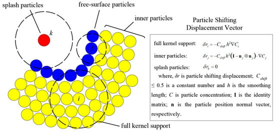
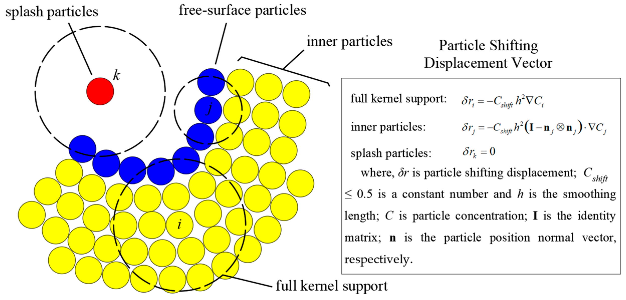
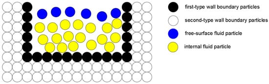
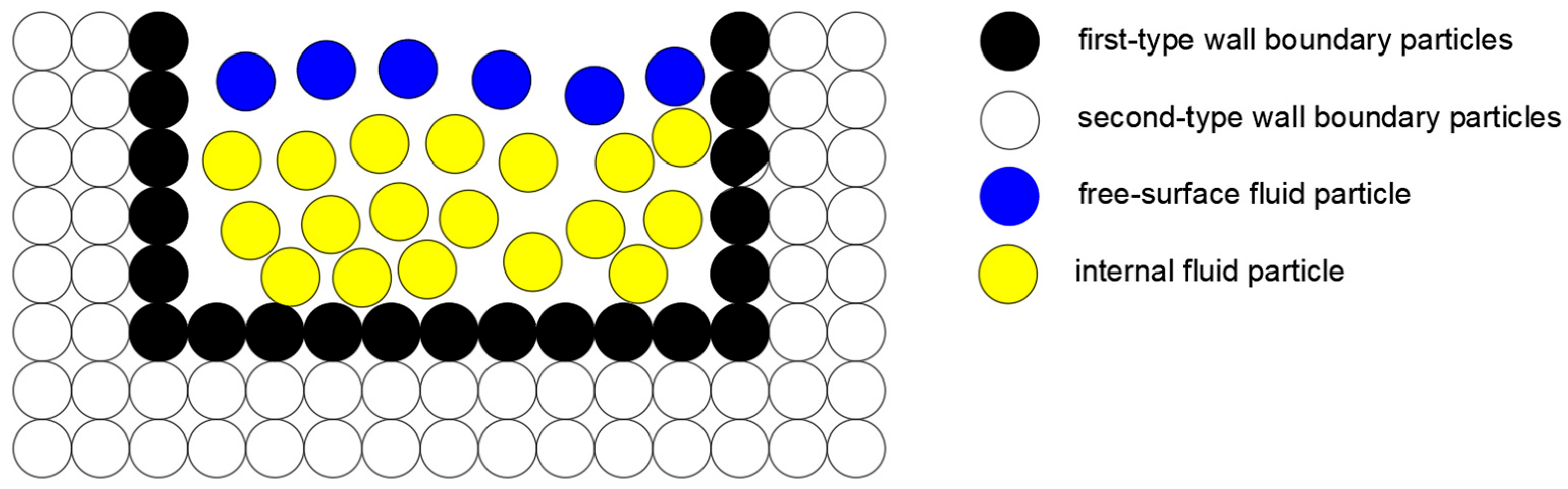
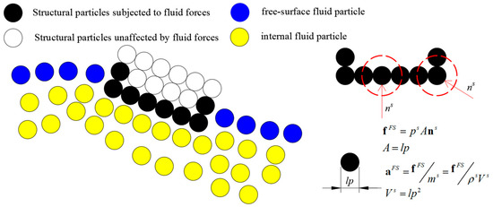
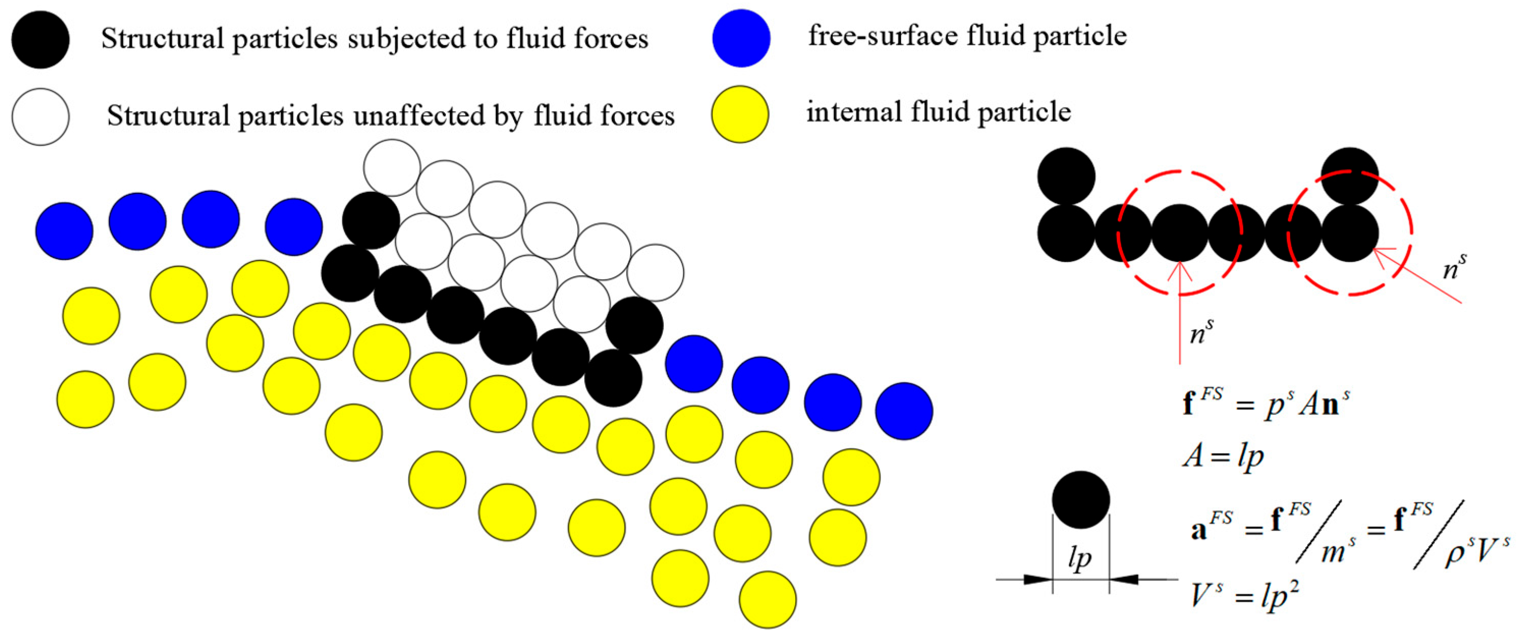
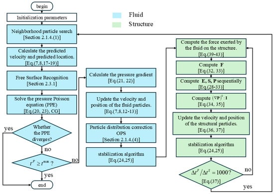
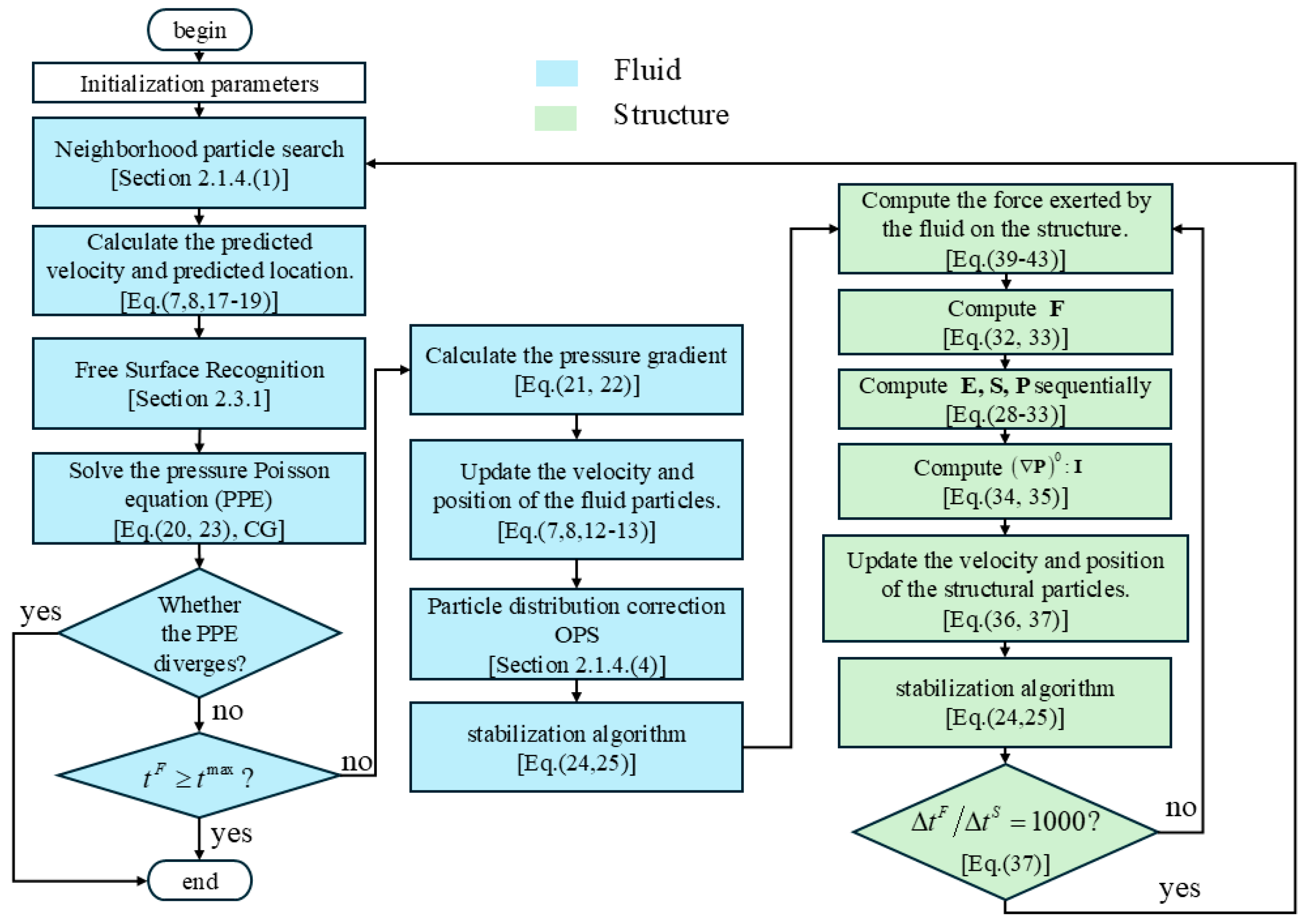
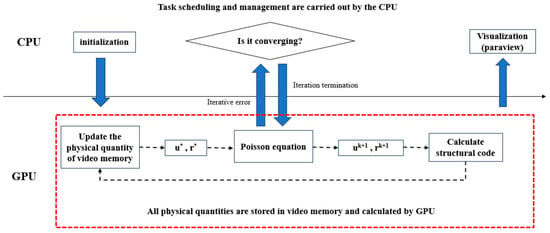
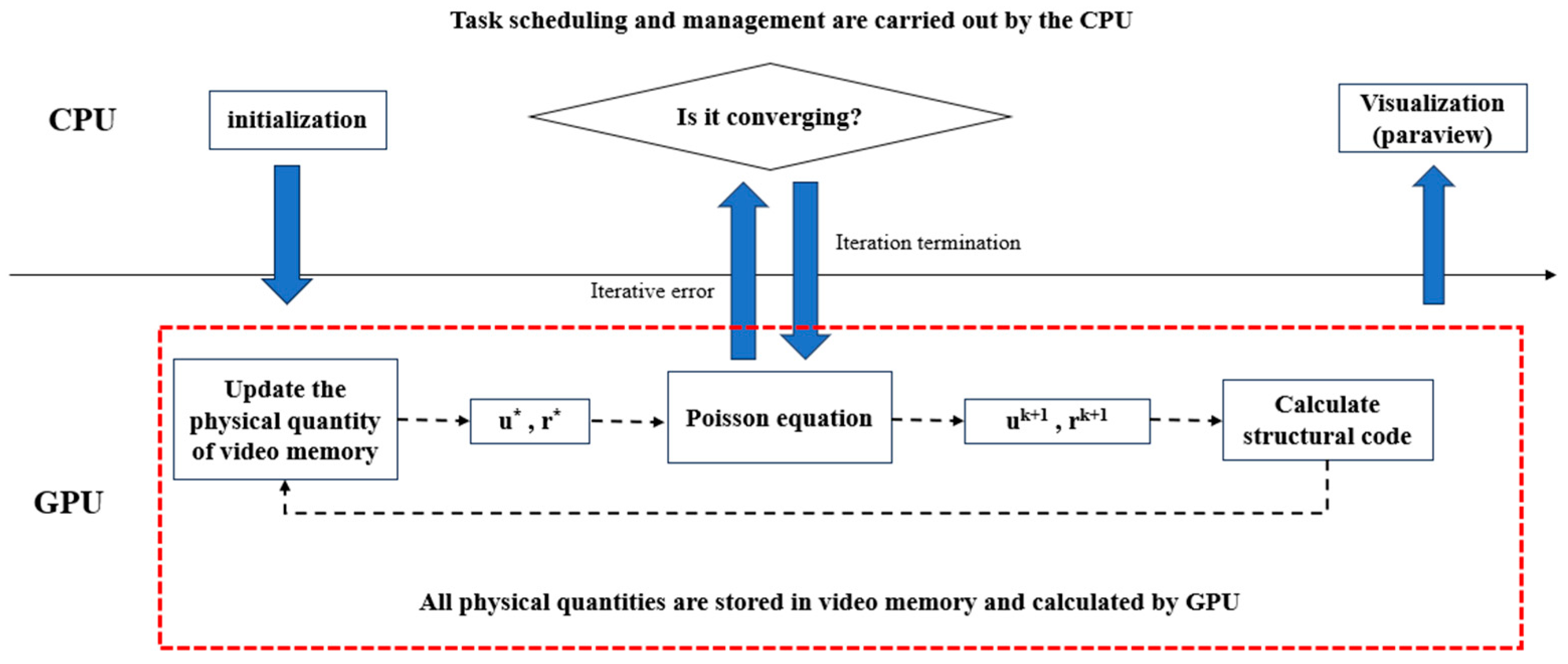
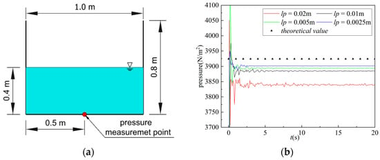
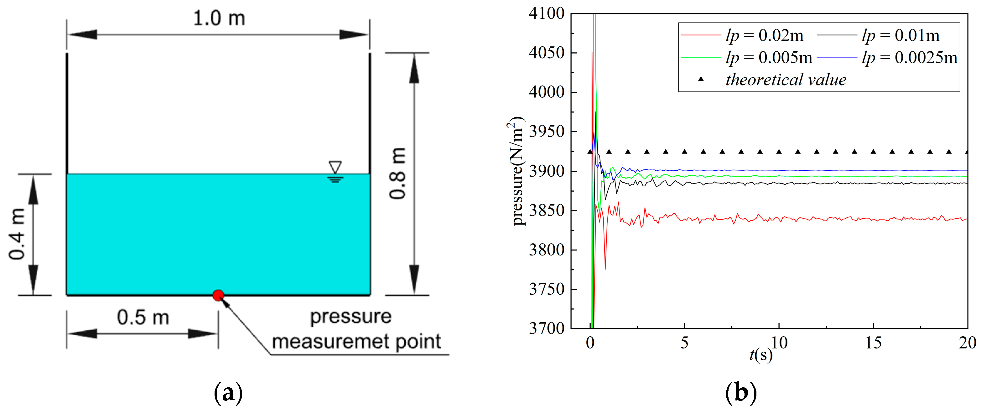
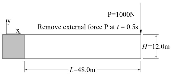
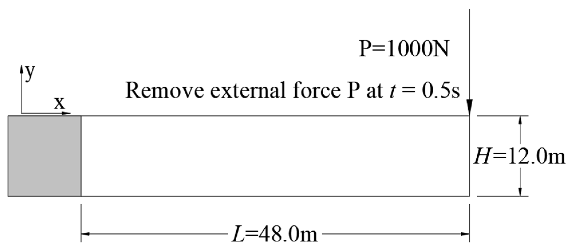
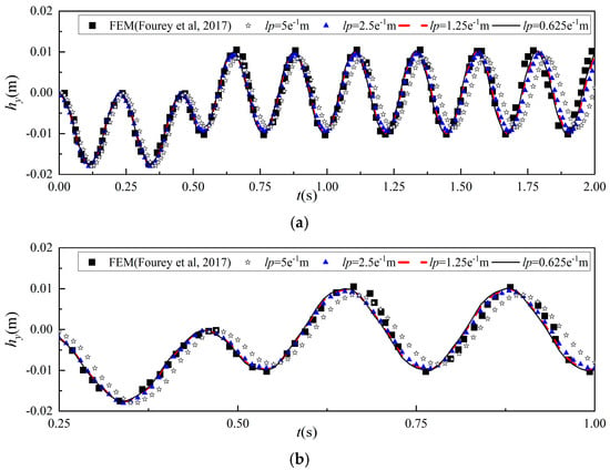
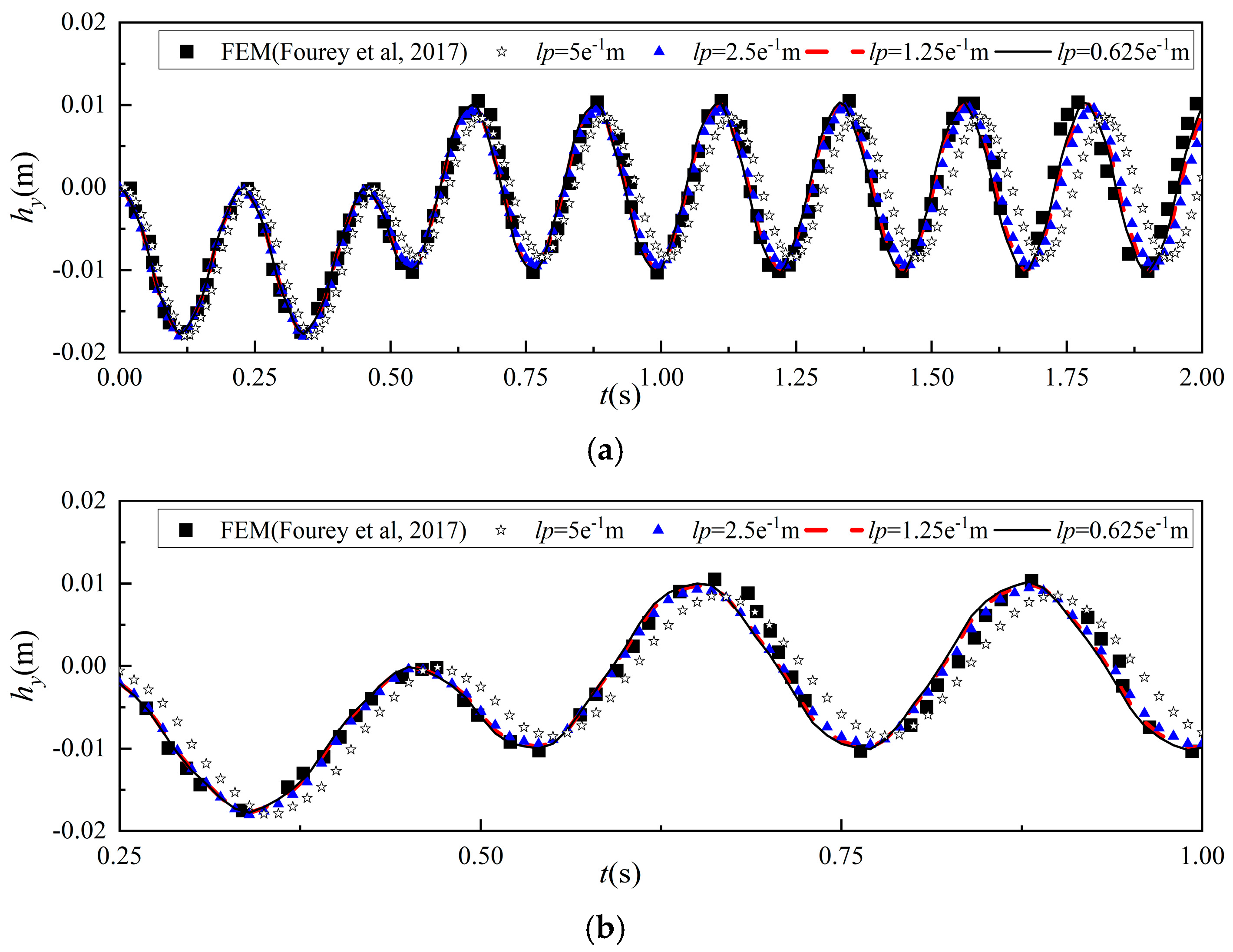
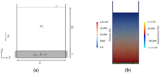
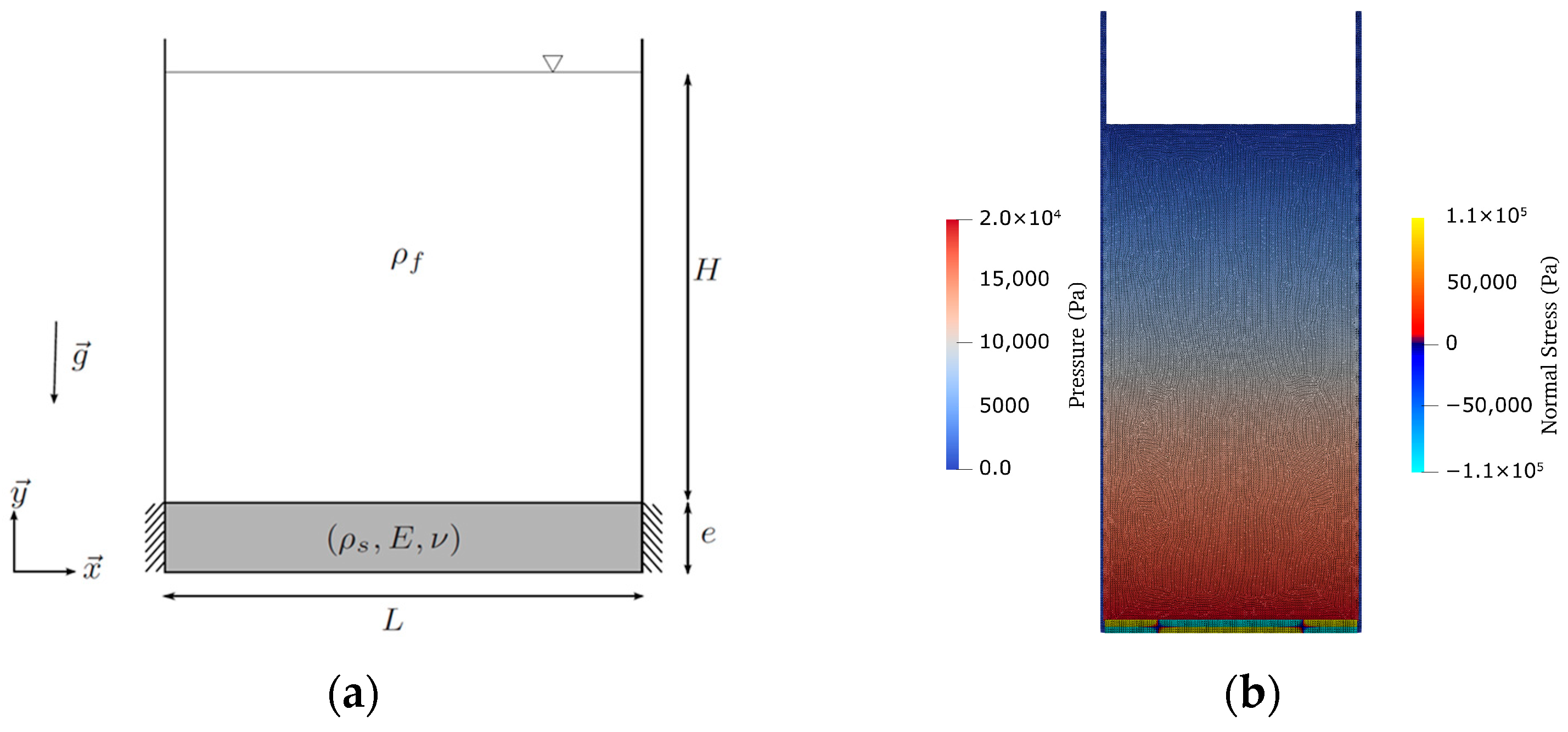
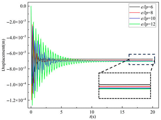
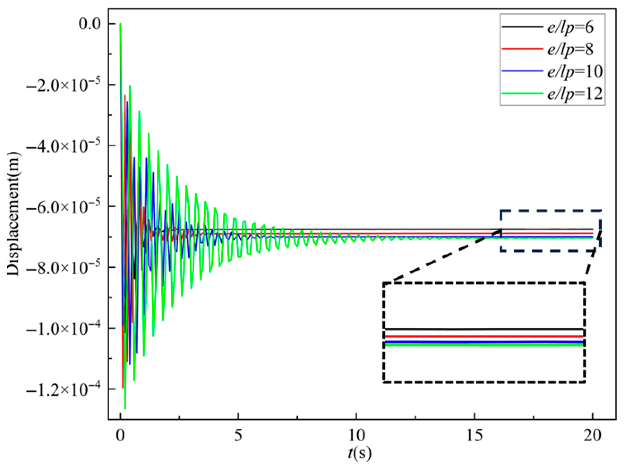
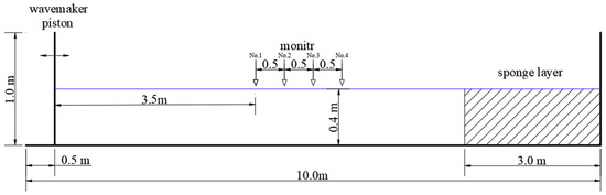
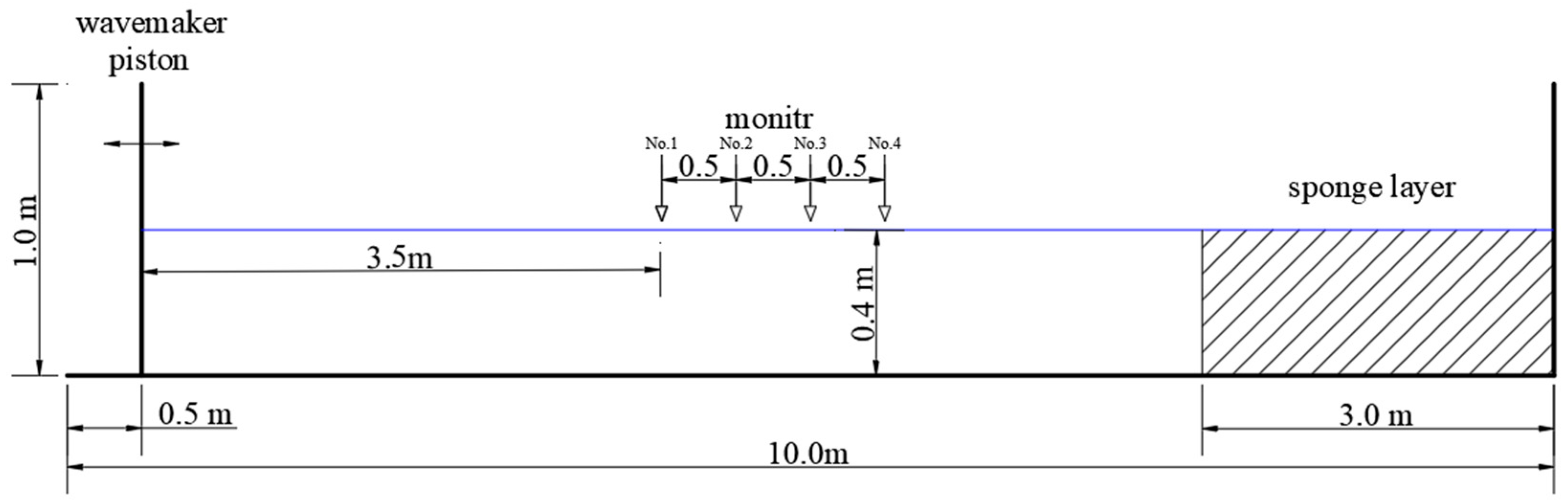
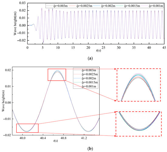
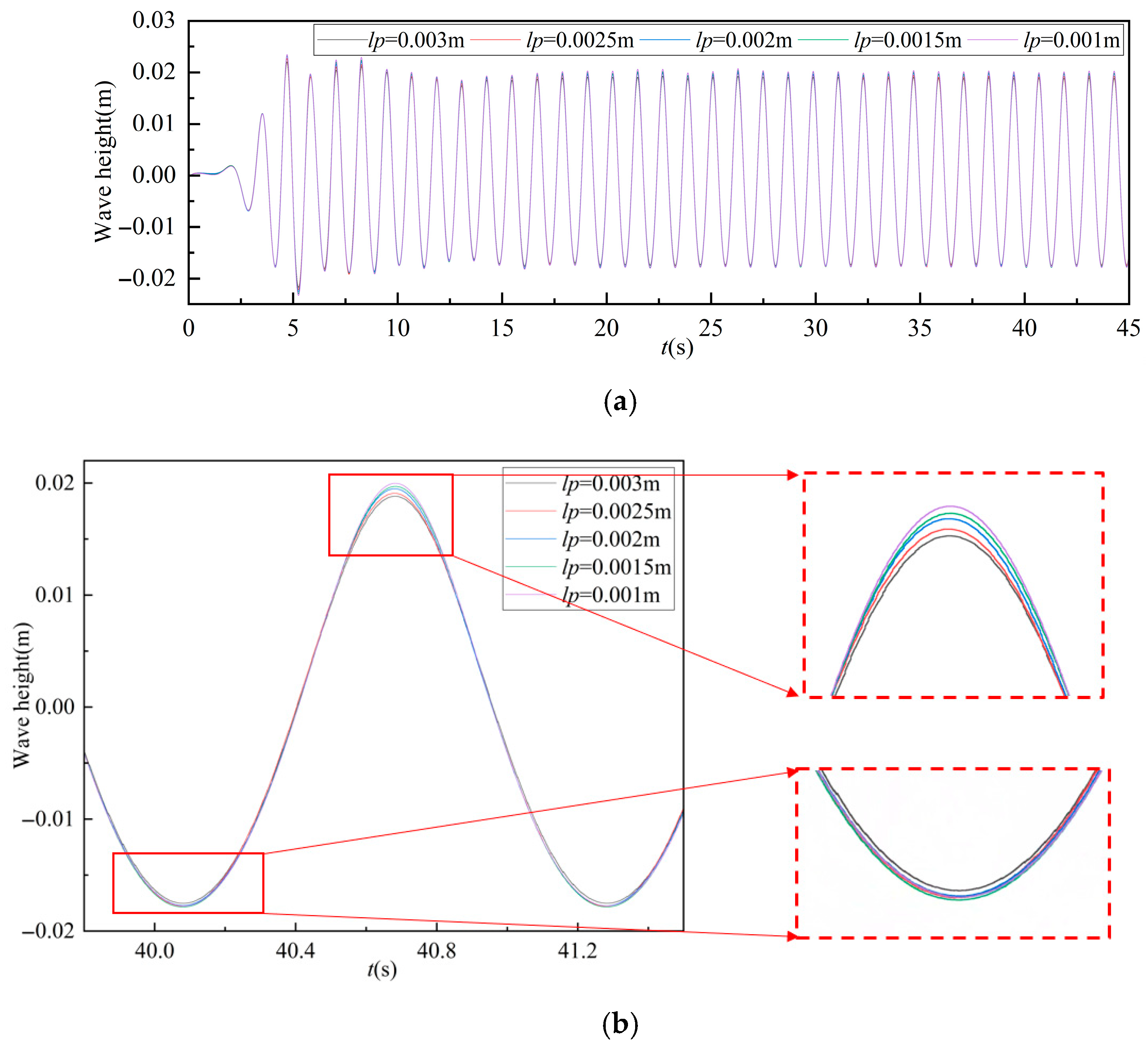
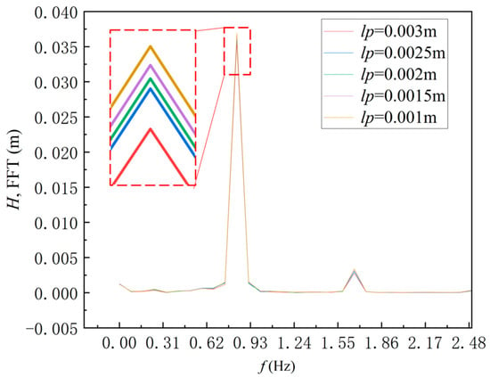
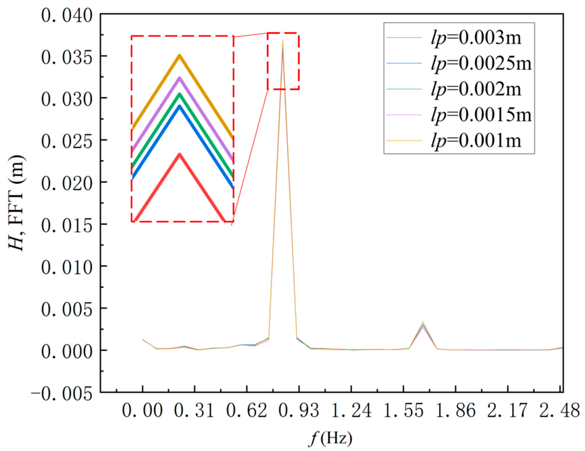
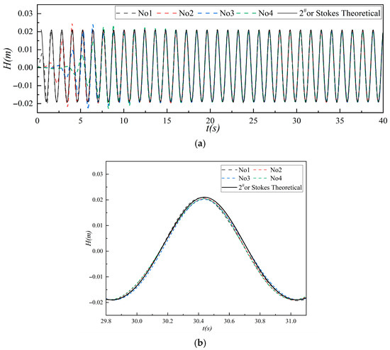
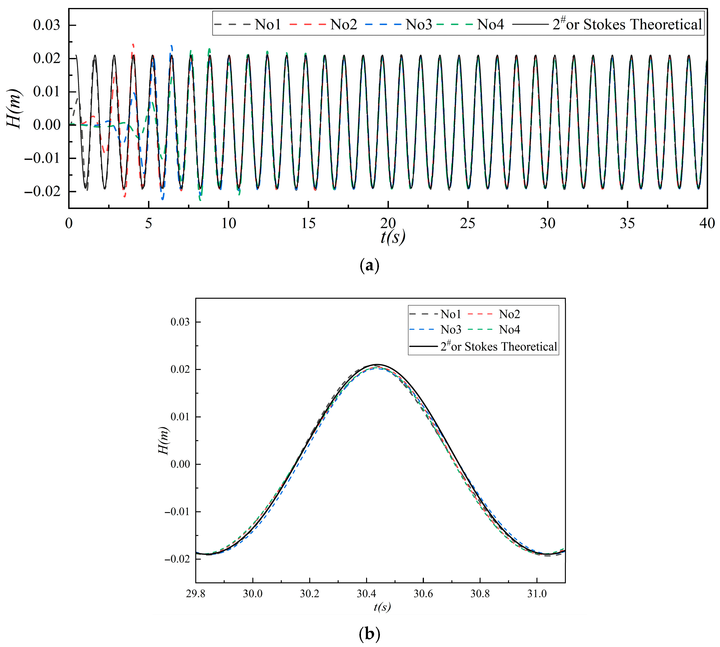
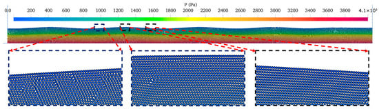
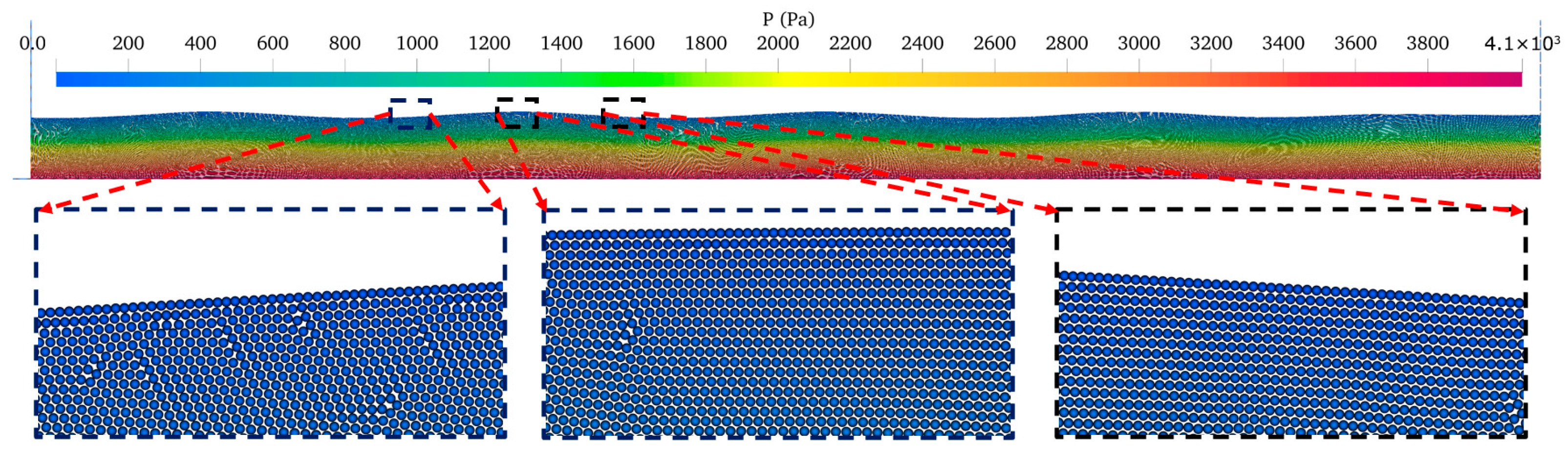
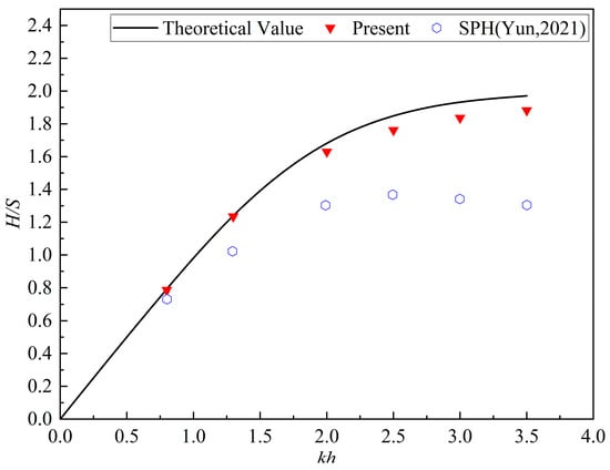
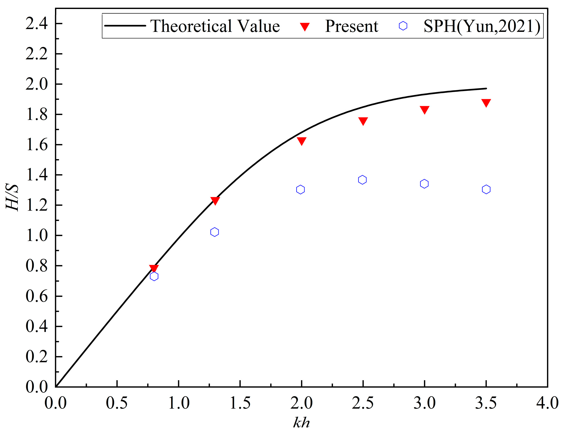
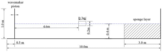
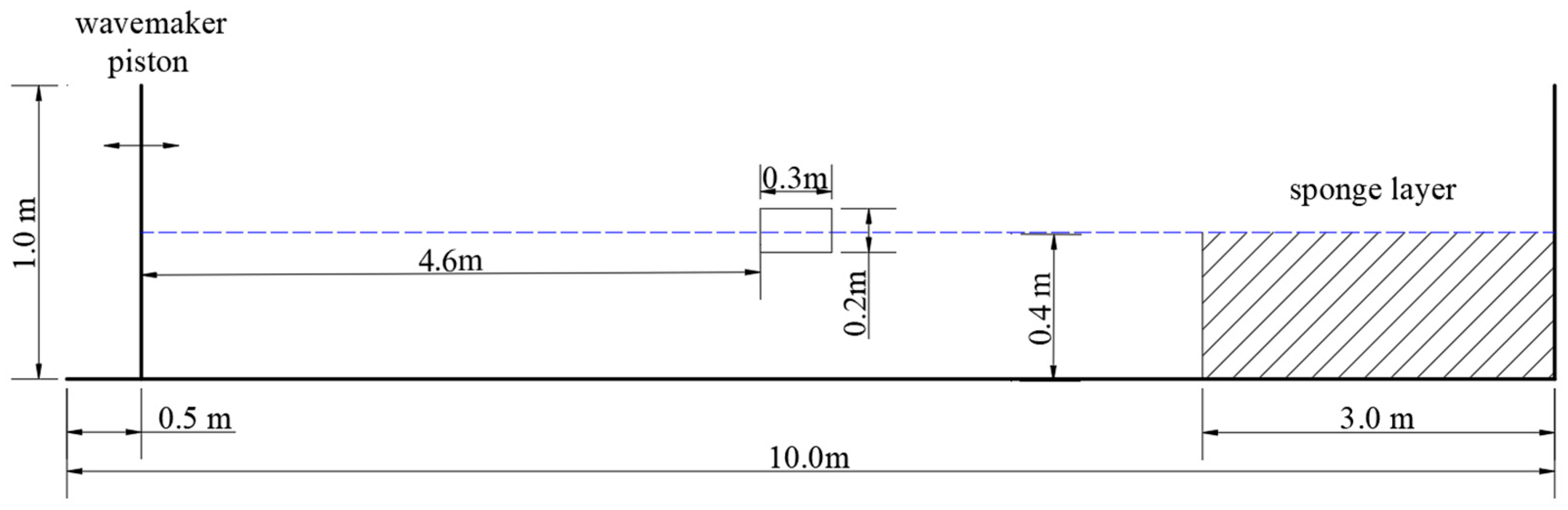
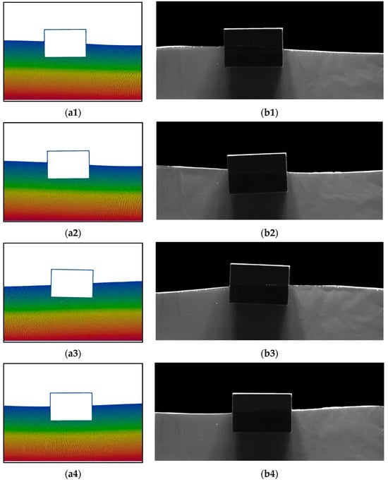
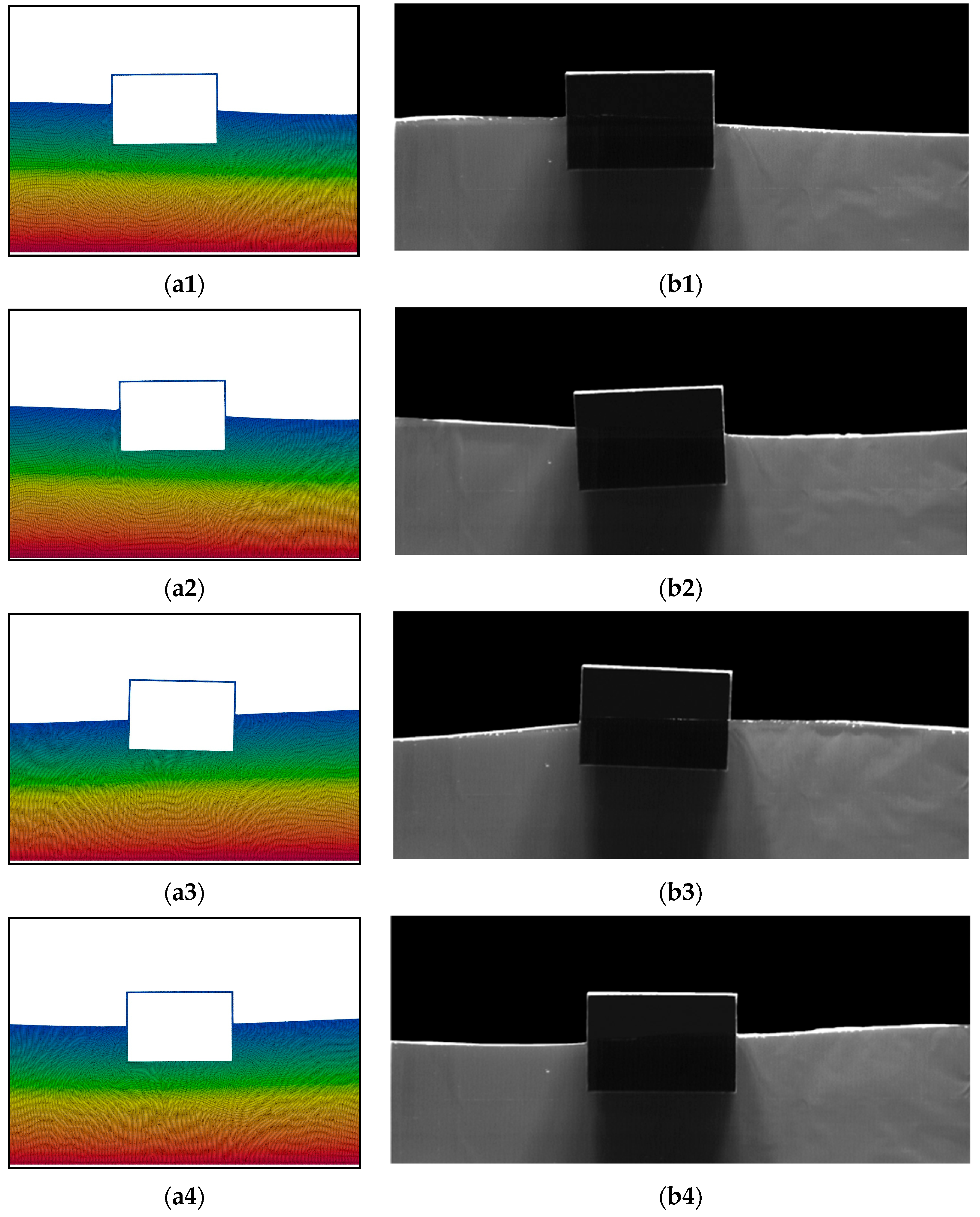
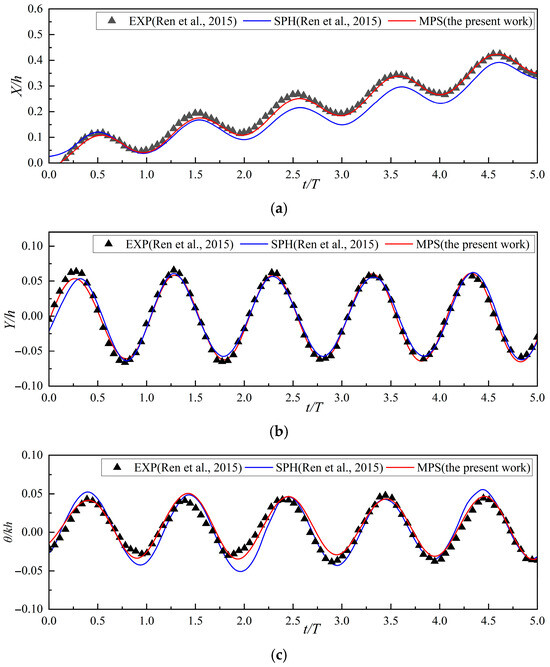
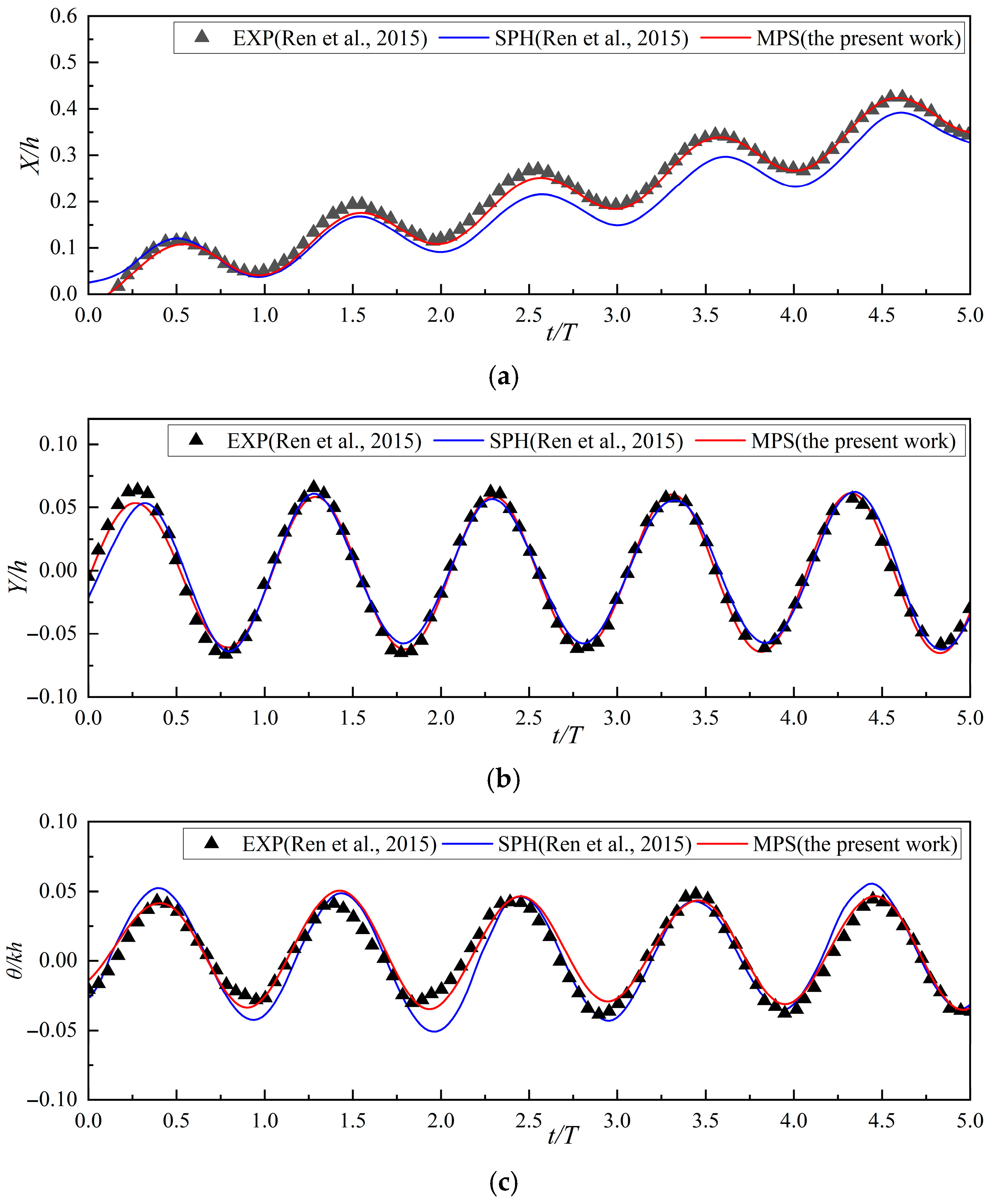
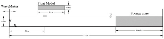
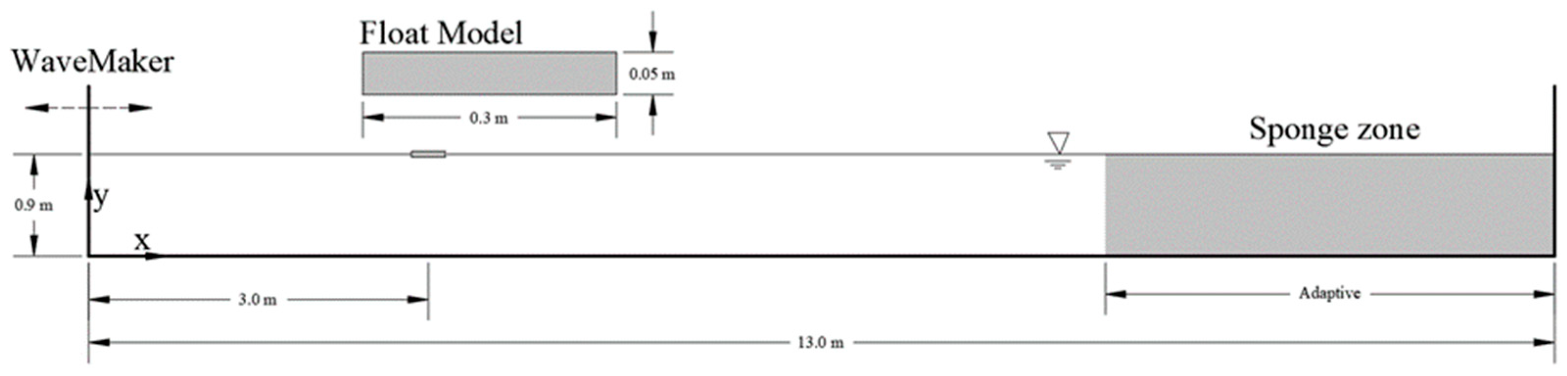
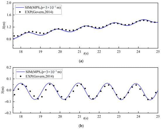
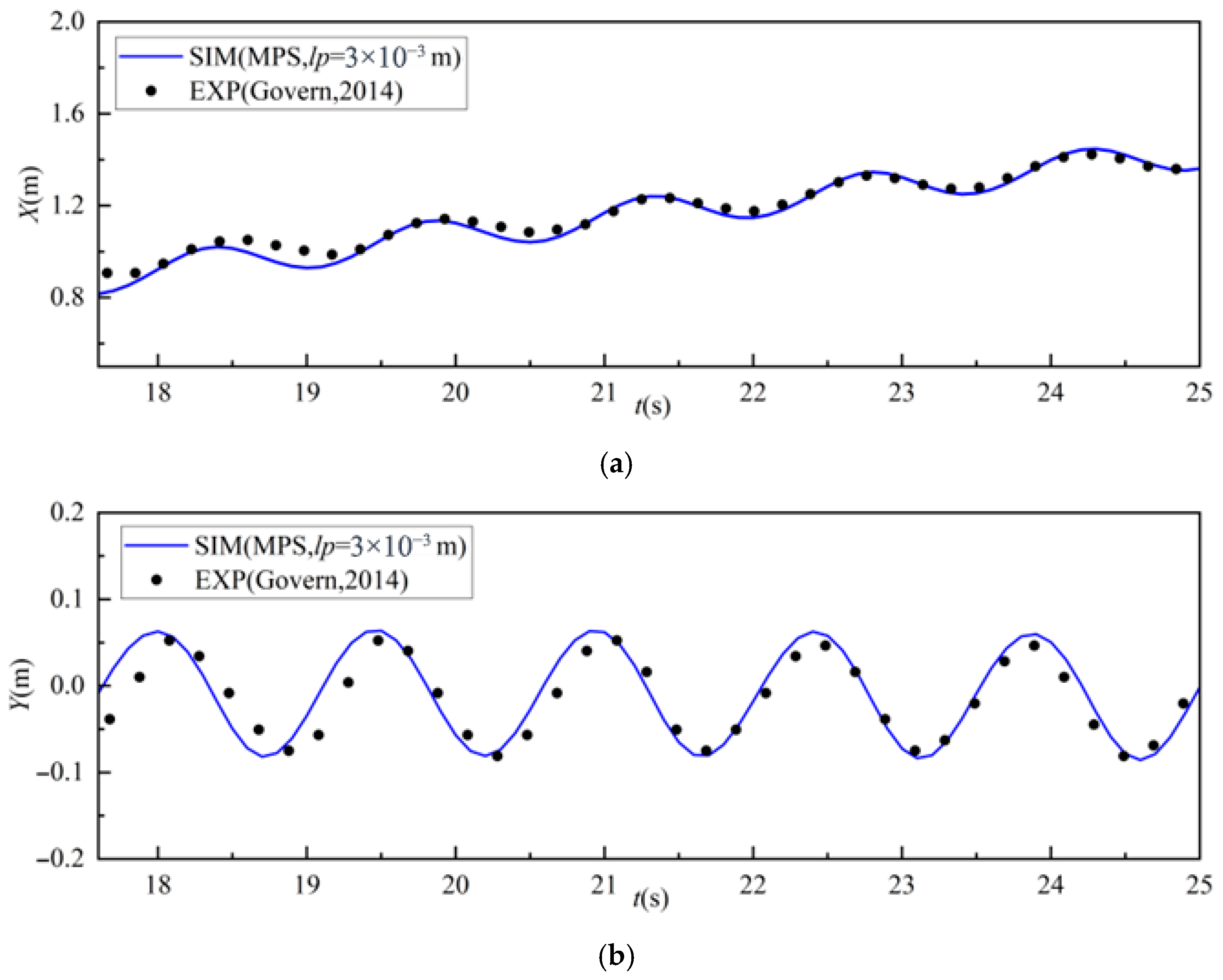
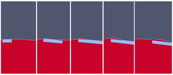
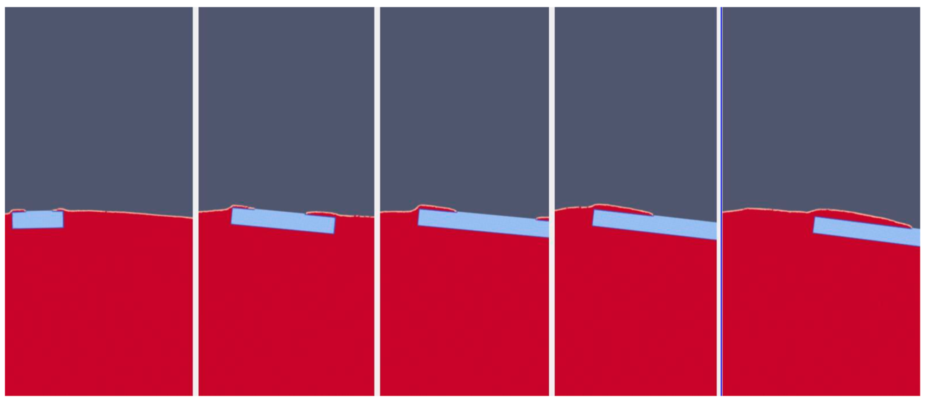
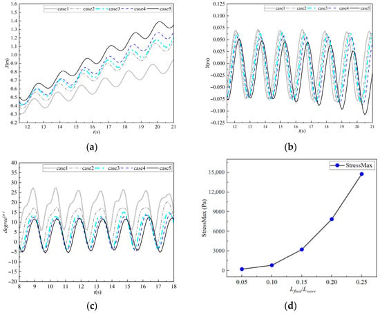
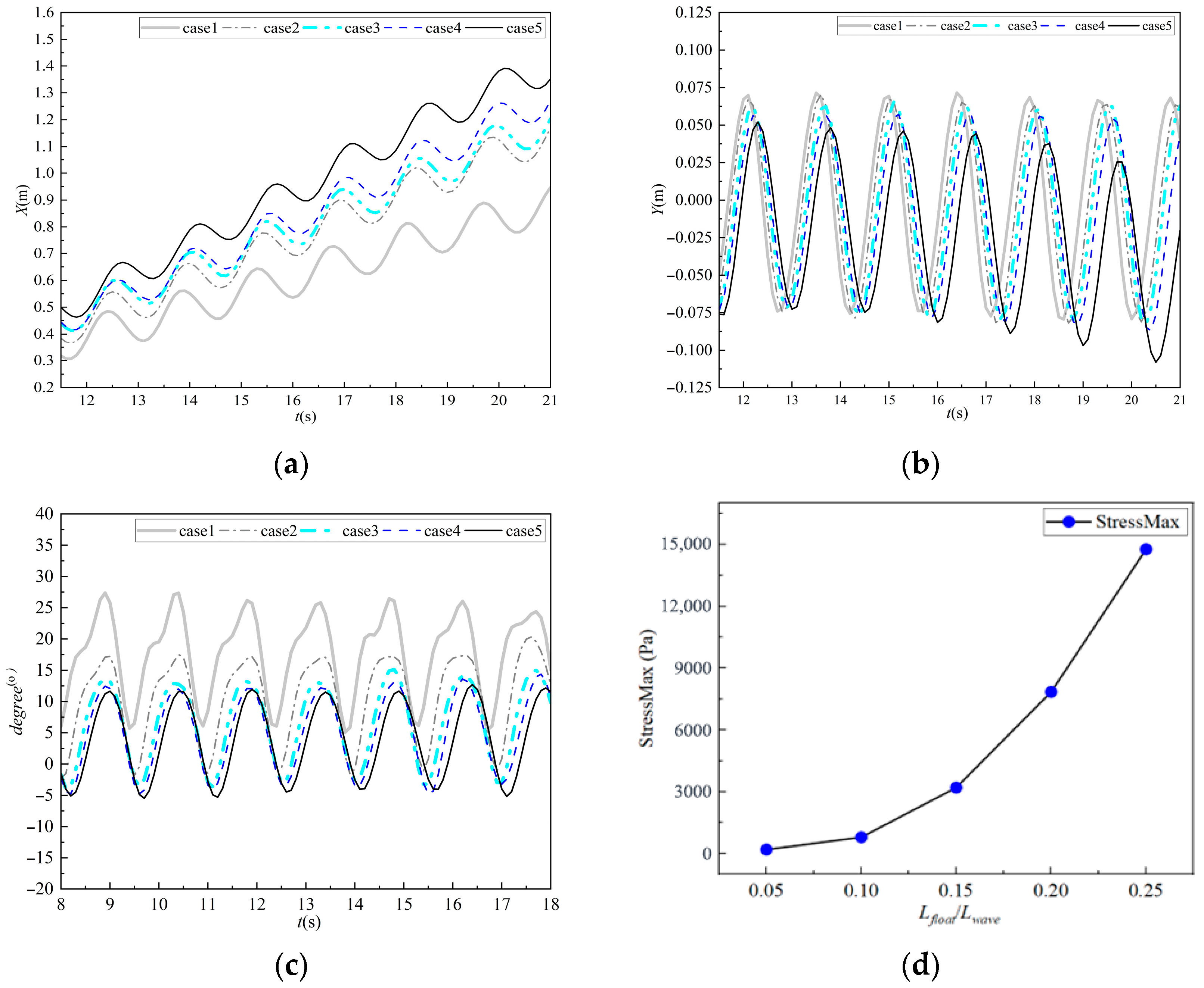
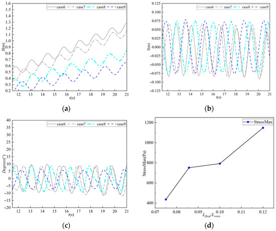
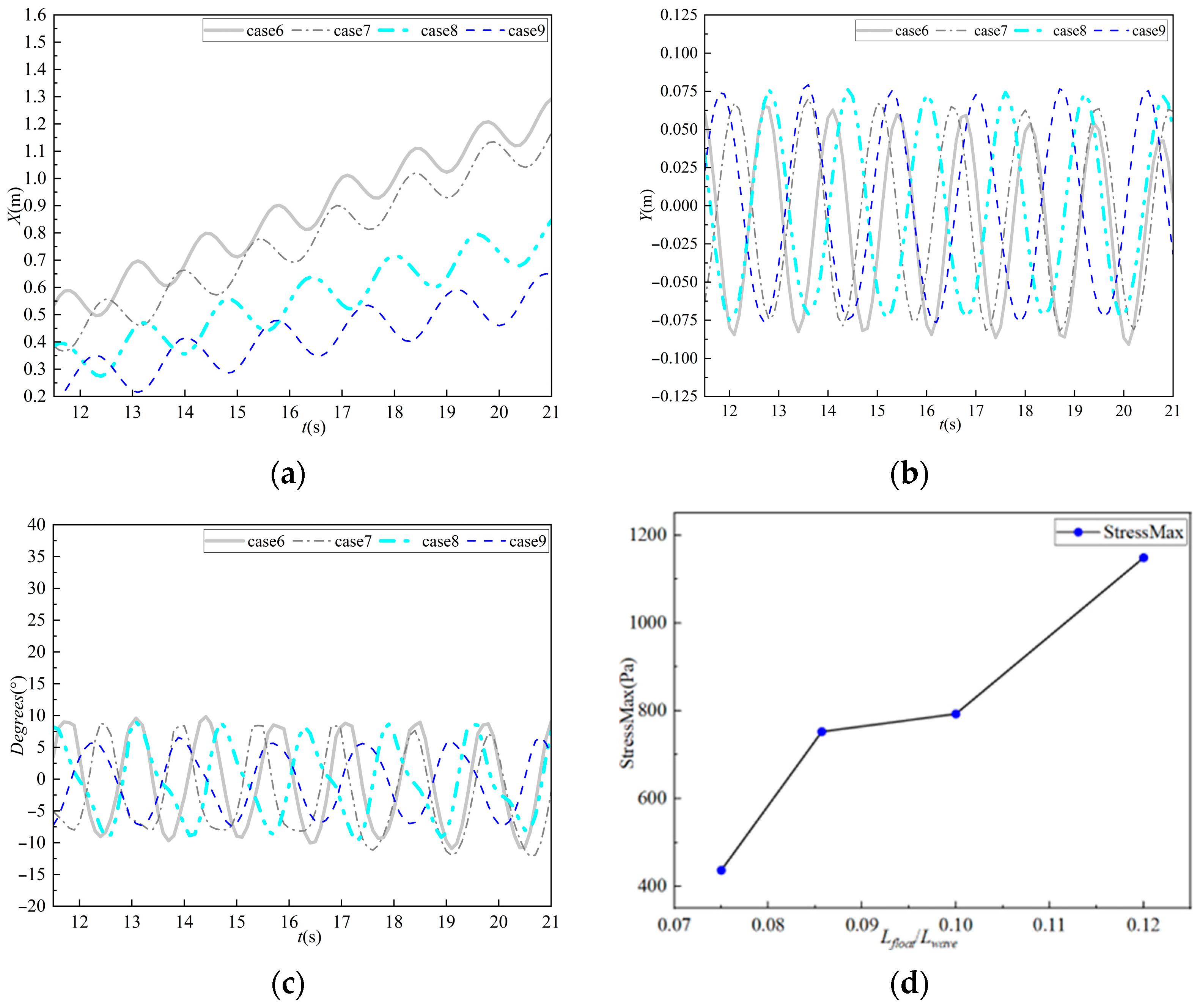
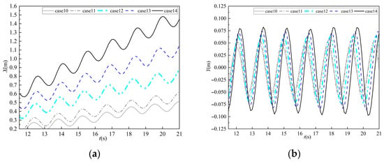
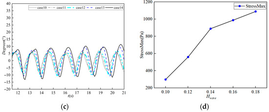
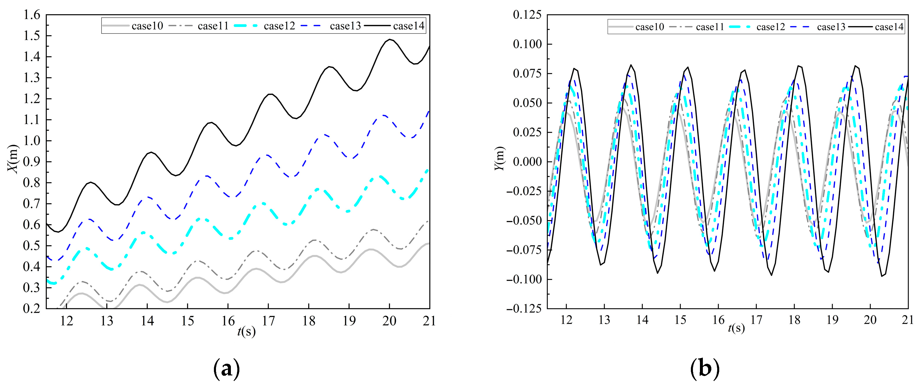
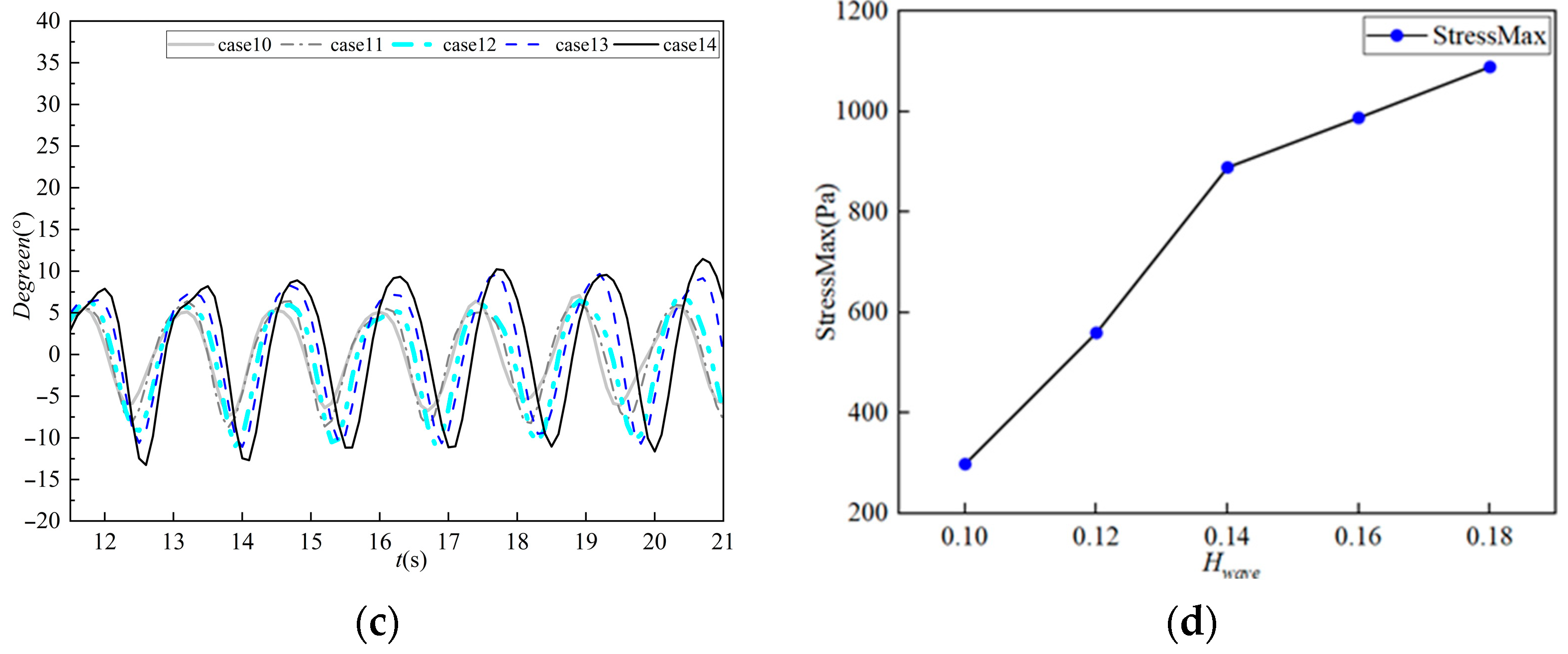

Disclaimer/Publisher’s Note: The statements, opinions and data contained in all publications are solely those of the individual author(s) and contributor(s) and not of MDPI and/or the editor(s). MDPI and/or the editor(s) disclaim responsibility for any injury to people or property resulting from any ideas, methods, instructions or products referred to in the content. |
© 2026 by the authors. Licensee MDPI, Basel, Switzerland. This article is an open access article distributed under the terms and conditions of the Creative Commons Attribution (CC BY) license.