


Abstract
Watershed Ecological Compensation (WEC) is a vital tool for water environmental governance, yet existing research often focuses on either upstream or downstream regions in isolation, lacking a systematic assessment of basin-wide aggregate effects. Taking China’s Xin’an River Basin as a case study, this paper investigates the impacts of cross-provincial WEC on pollutant emissions, economic performance, and green economic efficiency. Theoretical analysis based on a social welfare maximization framework indicates that WEC helps reduce emissions and enhance green economic efficiency, though its impact on economic output is conditional. Using the Synthetic Control Method (SCM) for empirical analysis, the results show that the policy significantly reduced industrial COD emissions by an average of 111 t/108 m3 per year and notably improved green economic efficiency, with industrial COD emissions per unit of GDP decreasing by 3.5 t per 100 million RMB annually. However, no significant impact on overall basin-wide economic development was observed. Robustness tests using Synthetic Difference-in-Differences (SDID) and staggered DID models further confirm the reliability of these findings. This study provides theoretical and empirical support for the policy effectiveness of WEC in pollution control and green development.
1. Introduction and Literature Review
The governance of watershed water pollution represents a core challenge to global sustainable development. The primary dilemma stems from the failure of coordination mechanisms across administrative jurisdictions. In the absence of effective institutional constraints, cross-border water management is prone to excessive emissions and the externalization of environmental costs, ultimately resulting in low overall governance efficiency [1]. This contradiction is particularly acute in developing countries and emerging economies. On one hand, improving water quality often requires local governments to restrict the scale of pollution-intensive industries, incurring high economic costs [2]. On the other hand, conflicting interests and the competition for development rights between different jurisdictions render traditional command-and-control measures ineffective [3]. Consequently, watershed governance essentially represents a cross-jurisdictional public goods supply problem characterized by inherent “free-rider” incentives [4], necessitating the exploration of incentive-compatible collaborative mechanisms.
To resolve this global governance dilemma, two primary institutional models have evolved internationally, though both possess limitations. The first is the command-and-control model, where governments intervene directly through mandatory regulations and standards. For instance, the U.S. Clean Water Act (CWA) mandates local governments to formulate pollution prevention plans and implement discharge permits [5], while the EU Water Framework Directive (WFD) enforces unified water quality targets through river basin management plans [6]. While highly binding, these systems face constraints related to negotiation costs, moral hazard, and enforcement difficulties [7,8,9], particularly in complex multi-stakeholder basins. The second is the market-based mechanism, which optimizes allocation through the trading of resources or environmental rights. Typical examples include water rights trading [10,11], emissions trading [12,13], and Payments for Ecosystem Services (PES) [14,15]. For example, Australia’s Murray–Darling Basin Plan establishes annual diversion limits and facilitates trading among users [16]. While flexible and efficient, these mechanisms are often limited to specific resource types and rely heavily on mature market and legal systems, restricting their applicability and effectiveness in coordinating multi-objective management in developing economies.
In response to the challenges of transboundary governance, China has pioneered a hybrid mechanism combining command-and-control with market incentives: Watershed Ecological Compensation (WEC) [17]. The core of this mechanism lies in the coordination by higher-level government, prompting upstream and downstream regions to forge contracts based on cross-section water quality targets. If water quality meets the target, the downstream region compensates the upstream; otherwise, the upstream indemnifies the downstream [18]. Theoretically, this system applies the concept of PES to basin-wide transboundary management [19], relying on central and local fiscal transfer payment systems for enforcement [20]. However, as it incorporates the “polluter pays” principle, it is not a pure PES but is described in the literature as a “PES-like” scheme [21,22]. This institutional arrangement reflects the adaptive selection of market-based tools within China’s centralized political–economic context, often interpreted as “authoritarian marketization” [22,23]. Since the launch of the first pilot in the Xin’an River Basin in 2012, the mechanism has expanded rapidly. As its coverage grows, determining whether WEC effectively achieves the multiple goals of pollution reduction, water quality improvement, and economic efficiency has become a focal point for both policymakers and scholars.
Under the WEC mechanism, the behavioral logic of upstream regions is driven by dual political and economic mechanisms. From a political economy perspective, in a multi-level governance system, administrative orders and performance evaluation pressure from higher-level governments are key drivers for lower-level environmental compliance [24,25]. When water quality targets are integrated into official promotion criteria, local officials tend to intensify environmental regulation to secure political advancement [26,27]. Empirical studies confirm that under the strong impetus of WEC, upstream governments increase environmental protection investment and compress high-pollution industries to meet contractual targets [28,29], thereby effectively reducing emissions and improving water quality [30]. From an environmental economics perspective, although the contract involves financial compensation, recipients only possess long-term economic incentives when compensation covers marginal abatement and opportunity costs [31,32]. However, in practice, upstream regions often undertake aggressive industrial restructuring and environmental investments to meet strict assessment standards. The actual governance costs frequently exceed the compensation received [23]. While this “cost–revenue inversion” objectively forces a green transition upstream [33,34], it simultaneously places substantial pressure on local fiscal stability and short-term economic growth.
In contrast to the arduous transition upstream, downstream regions occupy a relatively advantageous position in this asymmetric governance structure [35], yet the actual effects are complex. Theoretically, downstream jurisdictions benefit from the positive externalities of upstream governance [23,36]. Improved upstream water quality not only reduces downstream treatment costs [37] but also provides high-quality natural capital for developing high-value-added industries such as eco-agriculture and green tourism [38]. However, whether this “environmental dividend” translates into definite economic gains remains controversial; some empirical studies indicate that WEC has not significantly promoted aggregate economic growth downstream [28,34]. More critically, the mechanism may induce latent risks downstream: having fulfilled their financial compensation responsibilities, downstream governments may perceive a reduction in direct governance pressure [23]. This can lead to regulatory slack [28,34], potentially undermining the emission reduction effects of the basin as a whole.
Crucially, it must be recognized that China’s WEC mechanism is not a zero-sum game between upstream and downstream, but an institutional arrangement orchestrated by higher-level government [39]. For central decision-makers, the core objective is not to favor one party but to maximize total social welfare within the basin by correcting mismatched resources and responsibilities [40]. Despite this objective, existing empirical research typically focuses on either the abatement costs and fiscal pressure upstream or the water quality benefits and industrial dividends downstream, failing to assess the basin as an organic whole. An ecological compensation agreement is essentially a complex contract covering water quality targets, payment quotas, and industrial adjustments, the execution of which generates general equilibrium effects through upstream-downstream interactions. Analyses limited to a single regional perspective fail to capture the optimization of resource allocation and net welfare changes induced by the policy, limiting the generalizability of their conclusions. Just as environmental economics emphasizes analyzing market mechanisms like emissions trading within a general equilibrium framework, assessing cross-regional policies like WEC requires determining whether they enhance overall basin welfare [41]. Therefore, constructing a systematic assessment framework using the entire basin as the unit of analysis to identify the net effects on pollution, economic output, and social welfare is of significant theoretical and practical value.
Addressing this limitation, this paper takes the Xin’an River Basin in China as a case study, treating the upstream and downstream areas as a single entity. The study aims to systematically assess the combined impact of the mechanism on pollution, economic output, and green development, and to identify the net welfare gains for the entire basin. For this purpose. Based on a social welfare maximization framework, we first construct a welfare function encompassing pollution emissions, environmental quality, and economic output. This is used to derive the theoretical impacts of ecological compensation on overall pollution intensity, economic output, and green efficiency, proposing hypotheses for empirical testing. Subsequently, the SCM is employed to estimate the policy effects on pollution abatement, economic growth, and green efficiency, with the Synthetic Difference-in-Differences (SDID) model and staggered DID further used to test the robustness of the results.
This study contributes to the existing literature in three primary dimensions. First, this study contributes by shifting the analytical focus from localized assessments to a holistic welfare analysis. By integrating upstream and downstream regions into a unified framework, it moves beyond the conventional emphasis on distributive outcomes between regions and instead examines the net welfare gains of the entire watershed. This perspective better captures the collaborative nature of transboundary water governance, is more consistent with Pareto efficiency, and also extends the literature on “authoritarian marketization”. Second, this study deepens the analysis of policy mechanisms. Drawing on social welfare maximization theory, it develops a basin-wide welfare function that incorporates the interactions among water pollution emissions, water environmental quality, and economic output. This framework systematically reveals the transmission mechanisms and equilibrium effects of WEC and provides a more comprehensive tool for analyzing complex watershed governance policies. Third, this study contributes methodologically by combining the SCM, the SDID model, and staggered DID. This integrated strategy helps reduce estimation bias arising from heterogeneous treatment effects, strengthens causal identification, and offers a useful reference for evaluating similar water-related single-pilot policies.
2. Theoretical Analysis and Research Hypotheses
The economic theoretical analysis of WEC often relies on the PES theory proposed by Engel et al. [42]. In this theory, upstream regions shift from livestock farming to forest conservation, providing more environmental services to downstream regions and thus preventing downstream losses. In return, downstream regions compensate upstream areas, leading to increased economic benefits for both. Applied to WEC, this implies that appropriate compensation can reduce upstream pollution emissions and increase economic benefits for both upstream and downstream areas. However, the economic benefits in this theory are comprehensive and include various gains from environmental services, which may be oversimplified as economic output in empirical analysis. In fact, high environmental quality can directly provide utility to consumers and is often considered a luxury good, with demand increasing rapidly as economic development progresses [43]. Therefore, this study constructs social welfare functions that incorporate both pollution emissions and economic output for the two entities of upstream and downstream regions.
Consider a watershed that includes two regions, upstream and downstream, labeled as 1 and 2, respectively, as shown in Figure 1. Both regions regard pollution emissions as a production factor to obtain economic output, with the production functions represented as and , where is the production function, is the amount of pollution emissions, is the economic output, and indicates that the production technology level in the downstream region is not lower than that of the upstream region. The social welfare in the two regions depends on economic output and environmental quality, where the environmental quality is determined by the difference between environmental capacity and pollution emissions: , , . where is the social welfare function, represents social welfare, denotes environmental quality, represents environmental capacity, and indicates that pollution emissions from the upstream region flow downstream, reducing its environmental quality. The assumptions for the production functions and welfare functions include: , , , , , , . where the subscripts indicate first-order or second-order partial derivatives. It is assumed that the objective of both regions is to maximize social welfare.
Figure 1.
Pollution emissions and social welfare in upstream and downstream regions.
- (1)
- Theoretical Analysis Based on General Functions
First, analyze the baseline scenario where the upstream and downstream regions each maximize their own welfare. The welfare maximization problem for the upstream region is:
The optimal level of pollution emissions for the upstream region satisfies the first-order condition:
The welfare maximization problem for the downstream region is:
The optimal level of pollution emissions for the downstream region satisfies the first-order condition:
By solving Equations (2) and (4) simultaneously, the values for and can be obtained.
Next, analyze the target scenario of maximizing the overall welfare of the watershed. The total welfare of the watershed is the sum of the welfare of the upstream and downstream regions, and the maximization problem is:
The optimal levels of pollution emissions, and , satisfy the following two first-order conditions:
By solving Equations (6) and (7) simultaneously, the optimal pollution levels that maximize the overall welfare of the watershed, and can be obtained. Comparing the optimal emission levels under the two scenarios, it can be derived that: , , , . Additionally, in the optimization process, the optimal solution to one problem is generally not the optimal solution to another, resulting in: , , It can further be derived that . This indicates that compared to the scenario where the welfare of the upstream and downstream regions is maximized individually, when the overall welfare of the watershed is maximized, the upstream region experiences a reduction in pollution emissions, economic output, and welfare, while the downstream region sees an increase in pollution emissions, economic output, and welfare. Although the overall welfare of the watershed increases, it is difficult to determine the changes in the total pollution emissions and economic output for the entire watershed. These results are summarized in Table 1.
Table 1.
Comparison of overall welfare maximization and upstream-downstream welfare maximization results.
To achieve the outcome of maximizing the overall welfare of the watershed, the downstream region needs to pay an ecological compensation amount to the upstream region. Such payments would reduce the economic output and welfare of the downstream region while increasing those of the upstream region. Theoretically, there exists an appropriate range for the compensation amount that would make the welfare of both the upstream and downstream regions higher than under the scenario of individual welfare maximization. However, problems such as information asymmetry may cause the compensation amount to fall outside this suitable range, making it difficult to determine the changes in economic output and social welfare for both regions. These results are also summarized in Table 1.
- (2)
- Theoretical Analysis Based on Specific Functional Forms
To further calculate the total pollutant emissions and economic output in different regions, a detailed analytical derivation is necessary. Therefore, the general functions in the existing model are specified as concrete functions. Assume that production exhibits constant returns to scale, and the utility function follows a Cobb–Douglas form. Specifically, let: , ; , where is a parameter. For simplicity, we assume that , Both the upstream and downstream regions have identical environmental carrying capacities. Using these specific functional forms and under the first-order condition, the optimal emissions in two scenarios can be derived as: , , , . Comparing the results, we find , , which is consistent with the conclusions derived under general conditions. To further compare the total pollutant emissions and total economic output for the integrated regions, we can derive the following:
It is evident that for an integrated region, establishing a suitable ecological compensation mechanism will lead to a reduction in total pollutant emissions. This reduction depends on whether the environmental quality threshold is included in the utility function. If the environmental quality threshold is included (), the total emissions will decrease. However, if the environmental quality threshold does not enter the utility function (), total emissions will remain unchanged. At the same time, the change in total economic output is uncertain. Specifically, when , The total economic output will either increase, remain unchanged, decrease. Specifically, the condition for an increase in total economic output can be rewritten as , This condition implies that “the growth rate of the downstream region’s production technology relative to the upstream region” exceeds “the relative weight of environmental quality in the utility function”. In other words, if the downstream region’s production technology reaches a certain level, the total economic output will increase even as the total pollutant emissions in the basin decrease. This also implicitly assumes that payments from the downstream region to the upstream do not affect the total economic output or total welfare of the basin. These results are also presented in Table 1.
Welfare improvements are difficult to quantify and thus cannot be easily verified. Another method of combining pollutant emissions with economic output is the green economic efficiency, which is defined as the economic output per unit of pollutant emissions [44]. In the context of specific functional forms, we assume that the green economic efficiencies of both the upstream and downstream regions are fixed, meaning that WEC will not affect the green economic efficiency of either region. However, for the integrated basin, the green economic efficiency is:
By substituting the optimal emission levels under the individual welfare maximization scenario and into Equation (10), we obtain the baseline green economic efficiency:
Similarly, by substituting the optimal emission levels under the watershed welfare maximization scenario and into Equation (10), we obtain the optimized green economic efficiency:
Since , it can be derived that . This proves that when the overall welfare of the watershed is maximized, the aggregate green economic efficiency of the basin is higher compared to the decentralized baseline.
In the empirical analysis of the impacts of WEC practices, the actual amount of compensation paid may not necessarily equal the theoretical amount, making it challenging to predict the precise effects on upstream and downstream economic output and social welfare. However, as long as an WEC mechanism is established, qualitative conclusions regarding the overall watershed can still be drawn. Specifically, the total pollution emissions in the watershed are reduced, the total economic output depends on specific conditions, social welfare increases, and green economic efficiency is improved.
Based on the above theoretical analysis, the following hypotheses are proposed:
Hypothesis 1.
After the establishment of WEC, the change in the total economic output across the upstream and downstream regions of the watershed is uncertain.
Hypothesis 2.
After the establishment of WEC, the total pollution emissions across the upstream and downstream regions of the watershed will decrease.
Hypothesis 3.
After the establishment of WEC, the overall green economic efficiency across the upstream and downstream regions of the watershed will improve.
3. Research Design
3.1. Research Area
As a representative trans-provincial watershed, the Xin’an River Basin originates in Huangshan City (Anhui Province) and flows eastward into Hangzhou City (Zhejiang Province). Serving as the primary water replenishment source for the downstream Qiandao Lake, its water quality is critical to the water environmental security of the lake and the water supply security of Zhejiang Province [45]. In the early 21st century, accelerated industrialization and urbanization in the upstream region led to a substantial influx of pollutants into Qiandao Lake via the Xin’an River, triggering severe eutrophication issues, which can have serious impacts on aquatic ecosystems [46]. To address this transboundary governance challenge, the Ministry of Finance and the former Ministry of Environmental Protection issued the Implementation Plan for the Pilot of Water Environment Compensation in the Xin’an River Basin in 2011. Subsequently, in 2012, central ministries and the provincial governments of Anhui and Zhejiang formally signed the Xin’an River Basin Water Environment Compensation Agreement, marking the launch of China’s first trans-provincial WEC mechanism pilot. As a pioneering exploration and exemplary paradigm of China’s WEC institutional development [17], this case possesses significant research value and is therefore selected as the focal subject of this study.
The agreement established a bilateral compensation mechanism predicated on water quality targets. Adhering to the principle of “shared responsibility,” it stipulates that the downstream region compensates the upstream if water quality at the cross-boundary section meets the assessment standards, whereas the upstream indemnifies the downstream if standards are exceeded. To date, this mechanism has progressed through four rounds of implementation. The institutional evolution and specific funding arrangements for each round are detailed in Table 2.
Table 2.
Key content of the four-round ecological compensation agreement in the Xin’an River Basin.
3.2. Model Setup
To evaluate the overall effect of the Xin’anjiang WEC policy, this study adopts the SCM. This method constructs an optimally weighted combination of control units so that the synthetic group closely matches the characteristics of the treatment unit before policy implementation, and the post-policy difference between the two is then used to measure the policy effect [47,48]. Compared with the traditional difference-in-differences model, SCM does not rely on a strict parallel trends assumption and is more suitable when there is only a single treated unit.
The trans-provincial WEC in the Xin’an River Basin can be regarded as a quasi-natural experiment, where the combined region formed by Hangzhou City in Zhejiang Province and Huangshan City in Anhui Province serves as the treated group. Other regions that did not implement the policy act as the control group. In the SCM framework, suppose there are regions, where the first region is the treated group, and the remaining regions as the control group. The time period covers periods, with as the policy implementation time. Let represent the outcome variable of region at time , where , . To construct the counterfactual for the treated region, we denote as the outcome variable if the region had not been exposed to the policy, and as the outcome variable under the policy. Thus, when , , ; in other cases, . When , , is the policy effect:
To obtain the policy effect, we need to construct , which represents the predicted outcome for the treated region in the absence of the policy for . It is assumed that is determined by:
where is a vector of observable characteristics (i.e., predictor variables), is a vector of coefficients vector. The impact of on varies over time. The term denotes unobservable individual characteristics, while reflects the impact of on in different periods, changing over time. is a time fixed effect, and is a random disturbance term.
Let the weight vector used to construct the synthetic control group from the control group be denoted as:
where represents the weight of the -th region in the synthetic control group. Given the weight vector, the outcome variable for the synthetic control group can be expressed as:
By subtracting the above equation from , obtain:
For to be an unbiased estimate of , both and must be zero. However, since μ represents unobservable individual characteristics, it is difficult to determine whether their difference is actually zero. Abadie, Diamond and Hainmueller [48] demonstrated that if and , then . Therefore, if a weight vector can be found such that the outcome variables and predictor variables of the synthetic control group are similar to those of the treated group before the policy intervention, this weight vector will also ensure that the unobservable characteristics of the synthetic control group approximate those of the treated group.
In many cases, an exact solution that perfectly satisfies the system of equations may not exist, meaning that the synthetic control group may not perfectly match the treated group’s outcome variables and predictor variables before the intervention. Therefore, an approximate solution is used to determine the weight vector . Let the vector as weights, represents the possible linear combination of the outcome variables for each region in each period before the policy implementation. Let denote the set containing . Define the vector as the characteristic vector of the treated group before the intervention, where . Similarly, calculate the characteristic vector for each control region, and use these vectors as columns to form the matrix , representing the characteristic matrix for the control group before the intervention. The weight vector is chosen such that approximates as closely as possible. Given that each variable in may differ in its predictive power for the outcome variable, different weights can be assigned based on their predictive ability. The constrained minimization problem can be formulated as:
where and , thereby limiting the synthetic control group to a convex combination of the control units. Let be an diagonal matrix, where the diagonal elements are non-negative weights that reflect the relative importance of the corresponding variables for the outcome variable. The value of can be determined either exogenously or based on a data-driven approach. In this study, the data-driven method implemented in the Synth package for Stata, developed by Abadie, Diamond and Hainmueller [48], is used to calculate and obtain the optimal weight vector .
All empirical analyses in this study were conducted using Stata 18.0.
3.3. Sample and Variables
3.3.1. Selection of Sample Areas
In the SCM, the sample areas are divided into the treatment group and the control group. The treatment group consists of the Xin’an River Basin, which implements cross-provincial WEC, including Huangshan City in the upstream region and Hangzhou City in the downstream region. These two cities together form the experimental group. For the sake of readability, this section will refer to this combined area as Xin’an City.
The selection of the control group follows the principles of SCM and primarily consists of prefecture-level cities in Zhejiang and Anhui provinces that did not implement WEC [49]. Additionally, prefecture-level cities in Fujian with similar natural geographic and socio-economic conditions were included, while cities affected by administrative division adjustments were excluded. In total, 26 prefecture-level cities from the three provinces were selected as the control group.
3.3.2. Selection of Time Range
Although the first round of the Xin’an River Basin WEC pilot was implemented from 2012 to 2014, as early as 2010, the Ministry of Finance and the Ministry of Environmental Protection of China allocated 50 million RMB in startup funds to Anhui Province and issued an additional 200 million RMB in special funds in 2011. To mitigate potential early responses from the treatment group due to the anticipated policy [50], this study sets the policy implementation start year as 2010.
In setting the time window, this study distinguishes between the baseline identification period for the SCM and the extended observation period for long-run analysis. On the one hand, SCM requires a reasonable degree of comparability between the treated unit and the donor pool before and after policy implementation [51]. However, after 2016, with the issuance of the Guiding Opinions on Accelerating the Establishment of Horizontal Ecological Compensation Mechanisms for Upstream and Downstream River Basins, provinces across China gradually promoted intra-provincial horizontal WEC practices, which significantly increased the likelihood that potential control regions were exposed to similar policy interventions. By the end of 2019, 20 provinces (autonomous regions and municipalities) had basically established full-coverage ecological compensation mechanisms within their administrative river basins. This implies that mechanically extending SCM to later years would weaken the “untreated donor pool” assumption on which the method relies. For this reason, this study defines 2005–2015 as the baseline identification period for SCM, in order to identify the short- and medium-run effects of the policy.
On the other hand, because the diffusion of similar policies mainly occurred after 2016, its interference with the comparability between the treated unit and the donor pool during the baseline identification period is relatively limited. Accordingly, to further illustrate the long-run evolution of the policy effect, the SCM trajectories are extended to 2024, and 2015 is marked in the figures as the boundary between the baseline identification period and the extended observation period. At the same time, given that the likelihood of similar policy exposure among potential control regions increased after 2015, this study further employs a staggered DID model with the extended sample to formally estimate the long-run effects of the policy.
3.3.3. Selection of Outcome and Predictor Variables
Based on the basic theory of the SCM, this study selects variables from three dimensions to systematically assess the impact of the WEC policy:
In terms of economic development, Per Capita GDP is selected as the outcome variable to represent the regional economic development level. Labor, technology, and capital are essential production factors that determine economic growth and are closely related to the level of economic development. Therefore, we use the Employment Ratio, per capita human capital, and Per Capita Physical Capital as predictor variables for Per Capita GDP. Concurrently, to better predict the growth trend of Per Capita GDP, we also include the Tertiary Industry Share and Fixed Asset Investment Ratio as predictor variables to control for the similarity of the fitted results in terms of industrial structure.
For pollution emissions, the industrial COD emission index is selected as the outcome variable. Industrial COD emissions are an important indicator of water pollution [52]. However, directly using the total volume of industrial COD emissions may be influenced by differences in regional scale, thereby reducing comparability across regions. Considering that the impact of COD emissions on water quality depends not only on the amount of emissions itself, but also on the carrying capacity of the regional water environment, which is closely related to total water resources, this study constructs the industrial COD emission index as the ratio of industrial COD emissions to total water resources to capture the relative pressure of pollutant emissions on the local water environment. Specifically, total water resources are measured by the average annual water resources of each prefecture-level city over the period 2005–2015, so as to reduce the interference caused by annual fluctuations [53]. This indicator not only improves comparability across regions, but also more reasonably reflects the environmental impact of pollutant emissions. For predictor variables, economic-related variables are selected first. Because the level of economic development exhibits a positive relationship with pollution emission levels to some extent, we use Per Capita GDP to represent the economic variable. Second, relevant pollution emission variables are selected, as the discharge of related pollutants follows a somewhat similar pattern to the changes in the industrial COD emission index; here, we choose Per Capita Industrial Wastewater Discharge, which is highly relevant to watershed pollution. Finally, we select variables related to industrial structure. Given that pollution emissions primarily originate from the secondary industry, a similar industrial structure can ensure comparable development trajectories and help predict the future trend of the outcome variable. Therefore, we use the Secondary Industry Share as the industrial structure variable. In addition, this study also includes Industrial COD Emissions per Unit of GDP as a predictor variable to control for the coordinated development level between the economy and ecology.
In terms of green economic efficiency, Industrial COD Emissions per Unit of GDP is selected as the outcome variable to measure the pollution emission efficiency of the economic system. The predictor variables are selected primarily from three aspects: economic operation factors, industrial structure factors, and labor force quality, to ensure that the synthetic control group is highly similar to the experimental group in terms of green development potential. Specifically: for economic operation factors, Per Capita GDP and the Fixed Asset Investment Ratio are selected; for industrial structure factors, given that ecological pollution mainly originates from industry, the Secondary Industry Share is selected; regarding labor force quality, a high-quality labor force is often accompanied by higher environmental awareness and technological absorption capacity, thus Average Years of Education per Capita is selected as the predictor variable.
The basic descriptions of these variables are shown in Table 3.
Table 3.
Variable description and descriptive statistics.
3.4. Data Sources and Preprocessing
3.4.1. Data Sources
The industrial COD emissions data in this study primarily come from provincial and municipal statistical yearbooks. Data not listed in the yearbooks were supplemented by requests to the ecological and environmental authorities at the provincial and municipal levels. The data on average years of education per capita are sourced from the “2000 Census County-level Data,” the “2010 Census County-level Data,” and relevant population censuses, sample surveys, and statistical yearbooks from provinces such as Zhejiang and Anhui. Data for other variables are derived from the statistical yearbooks of the three provinces and their respective prefecture-level cities.
3.4.2. Data Preprocessing
Data preprocessing mainly includes price deflation, estimation of physical capital stock, and the synthesis of data for Xin’an City, along with adjustments and imputation of missing or outlier values using linear interpolation.
For price deflation, all monetary data were adjusted to constant prices with 2005 as the base year, using the corresponding price indices to eliminate the impact of price fluctuations. The estimation of physical capital stock was done using the perpetual inventory method, converting fixed asset investments into comparable real capital stock.
The data for Xin’an City were synthesized by combining data from Hangzhou and Huangshan cities. Specifically, total indicators were directly summed from the corresponding data of the two cities, while per capita or ratio indicators were weighted based on population and other variables to accurately reflect the overall characteristics of the region.
4. Empirical Results
4.1. Economic Development Effects
The SCM results indicate that the synthetic Xin’an City is constructed from a weighted average of three donor cities. The weights, in descending order, are Shaoxing (0.472), Xiamen (0.296), and Jiaxing (0.232). Table 4 presents the pre-policy average values of the economic predictors for the actual Xin’an City, the synthetic Xin’an City, and the average of all other cities in the donor pool. The predictor values for the synthetic Xin’an City closely approximate those of the actual Xin’an City. Notably, the disparities between the actual and synthetic counterparts are considerably smaller than those between the actual Xin’an City and the average of other cities, suggesting that our synthetic control group accurately replicates the economic growth trajectory of Xin’an City prior to the policy intervention.
Table 4.
Predicted variable values for economic development in Xin’an City and synthetic Xin’an City.
Figure 2 reports the dynamic changes in per capita GDP between Xin’an City and its synthetic counterpart. Before policy implementation, the trajectories of the treated unit and synthetic Xin’an City largely overlap, indicating a good pre-intervention fit of the SCM. Using 2010 as the policy intervention year, the difference between the actual and synthetic values can be interpreted as an estimate of the policy effect. The results show that during the baseline identification period of 2010–2015, the deviation between the two remains relatively small and does not evolve into a persistent or meaningful gap, suggesting that the WEC policy had no clear short- or medium-run effect on per capita GDP in Xin’an City.
Figure 2.
Comparison of per capita GDP between Xin’an City and synthetic Xin’an City.
Furthermore, the SCM trajectories are extended to 2024 to examine the long-run evolution of the policy effect. The results show that during the post-2015 observation period, although some fluctuations are observed between the treated unit and the synthetic control, no persistent and systematic divergence emerges overall. Descriptively, these extended trajectories do not suggest a persistent growth-promoting effect on per capita GDP in Xin’an City. Instead, the long-run influence of the policy may be better understood as a gradual adjustment in the development path rather than a marked increase in per capita GDP.
4.2. Pollution Emission Effects
The synthetic control for Xin’an City is composed of four cities: Xiamen (w = 0.486), Shaoxing (w = 0.298), Chizhou (w = 0.215), and Zhangzhou (w = 0.001). As shown in Table 5, the pre-intervention characteristics of the synthetic unit closely match those of the actual Xin’an City. Although a slight divergence is observed in the share of the secondary industry, the overall fit of the synthetic control is significantly superior to the average of the unweighted donor cities. These results confirm that the synthetic control provides a credible counterfactual for the trajectory of industrial COD emissions in Xin’an City before the policy intervention.
Table 5.
Predicted variable values for pollution emissions in Xin’an City and synthetic Xin’an City.
The SCM results are presented in Figure 3. Before policy implementation, the trajectories of the industrial COD emission index for Xin’an City and synthetic Xin’an City are broadly consistent, indicating a good pre-intervention fit of the treated unit’s pollution trend. Using 2010 as the policy intervention year, the actual value becomes markedly lower than the synthetic value, suggesting that the WEC policy reduced industrial COD emissions in Xin’an City. As shown by the gap results, during the baseline identification period of 2010–2015, the difference between the two widens rapidly and remains negative, with the industrial COD emission index declining by an average of 111 t/108 m3 during 2010–2015. This pattern suggests that the policy generated a substantial industrial pollution-abatement effect in its initial and intermediate stages.
Figure 3.
Comparison of industrial COD emission index between Xin’an City and synthetic Xin’an City.
Extending the trajectories to 2024 further shows that during the post-2015 observation period, the gap between the treated unit and the synthetic control remains negative overall, suggesting that the pollution-reduction effect persists to some extent; however, its absolute magnitude declines relative to the initial post-policy years. In light of the institutional background, this change may be related to the gradual expansion of intra-provincial horizontal WEC practices after 2016. As some potential control regions may also have strengthened pollution control under similar policy arrangements, the relative pollution-reduction advantage of the treated unit over the synthetic control may have narrowed. Therefore, the post-2015 SCM trajectories should be interpreted mainly as descriptive evidence on the long-run evolution of the policy effect, while formal identification of long-run effects relies on the staggered DID estimates that additionally control for prefecture-level WEC policies.
To further test the significance of the policy effect, this study applied the placebo test method proposed by Abadie, Diamond and Hainmueller [48]. The core idea of this method is to hypothesize that all the cities in the control group that did not implement the policy also “implemented” the policy. Each control city is sequentially treated as a synthetic treatment group, and its synthetic control group is constructed to calculate the corresponding “treatment effect”. Then, the policy effect of the actual treatment group is compared with the effects of all these synthetic treatment groups. If the actual effect is significantly larger than most of the effects generated by the synthetic treatment groups, it indicates that the policy’s impact is not likely due to chance.
The placebo test results are reported in Figure 4. Based on the goodness of fit in the pre-policy period (2005–2009), regions with poor pre-treatment fit are excluded, leaving 11 prefecture-level cities in the comparison sample. The results show that before policy implementation, the estimated treatment effects across cities fluctuate around zero, and Xin’an City does not exhibit systematic differences from the other regions. After policy implementation, however, especially during the baseline identification period of 2010–2015, the estimated treatment effect for Xin’an City declines sharply and is clearly lower than those of the other placebo samples, indicating that the reduction in its industrial COD emission index is larger than that of most control regions. According to the logic of the placebo comparison, the probability that the treatment effect for Xin’an City is driven by random factors is only 1/12 (approximately 8.33%), suggesting that the industrial pollution-abatement effect of the WEC policy is statistically meaningful. After 2015, the treatment effect for Xin’an City remains lower than that of most placebo samples, suggesting that the pollution-reduction effect continues in the longer run, although its relative advantage becomes less pronounced than during the baseline identification period.
Figure 4.
Treatment effect on pollution emissions in Xin’an City and other regions. The black line represents Xin’an City, and the gray lines represent the placebo-treated regions.
Another method to enhance the robustness of statistical inference is to examine the distribution of the ratio of root mean squared prediction errors (RMSPE) before and after the policy intervention [46]. This approach measures the relative strength of the policy effect by calculating, for each region, the ratio of “post-intervention RMSPE” to “pre-intervention RMSPE”. The underlying logic is that, if the policy has had a significant effect, the prediction error for the treated group should increase substantially after the intervention compared with before it; by contrast, for control groups not exposed to the policy, prediction errors should remain relatively stable over time. Moreover, using the ratio rather than the absolute prediction error helps effectively eliminate statistical bias arising from poor pre-intervention fit in some samples (i.e., a large initial RMSPE), thereby allowing for a more objective assessment of the significance of the policy effect.
It should be noted that the RMSPE ratio test is conducted within the baseline identification window of 2005–2015. This is because the test is designed to evaluate the relative change in model fit before and after the implementation of the initial WEC pilot. If the extended observation period of 2016–2024 were included, the gradual expansion of intra-provincial horizontal WEC practices across regions could also affect some potential control areas. This would in turn change the error distribution and ranking of the placebo samples, weakening the test’s ability to isolate the net effect of the initial pilot. Therefore, the 2005–2015 sample period is retained in the RMSPE ratio test to ensure consistency and comparability with the baseline SCM estimates.
Figure 5 presents the distribution of RMSPE ratios for pollution emissions across all cities during the sample period. The results show that Xin’an City has an RMSPE ratio of 102.60, ranking first among all samples and far exceeding that of the second-ranked city, Shaoxing (17.55). This implies that the probability that the observed emission-reduction effect in Xin’an City was driven by random factors is only 1/26, or 3.85%. Accordingly, the null hypothesis that the observed effect was caused by random variation can be rejected at the 5% level. Taken together, the placebo test and the RMSPE ratio ranking test consistently suggest that the WEC policy generated a significant and robust emission-reduction effect.
Figure 5.
Post/pre pollution emissions mean squared prediction error.
4.3. Green Economic Efficiency Effects
The synthetic control for Xin’an City relies on four cities from the donor pool: Shaoxing (w = 0.425), Nanping (w = 0.292), Xiamen (w = 0.214), and Chizhou (w = 0.069). To optimize the model fit, we followed the methodology of Abadie, Diamond and Hainmueller [48] by including the 2009 industrial COD emissions per unit of GDP (the immediate pre-policy year) as a predictor. As shown in Table 6, the pre-intervention characteristics of green economic efficiency for the synthetic Xin’an City demonstrate a strong fit with the actual city. While the fixed asset investment rate shows some divergence, the deviation between the actual and synthetic units remains considerably smaller than the disparity observed between the actual city and the unweighted average of other cities. These results confirm that the constructed synthetic control provides a valid counterfactual for the green economic efficiency of Xin’an City before the policy implementation.
Table 6.
Predicted variable values for green economic efficiency in Xin’an City and synthetic Xin’an City.
The SCM results are shown in Figure 6. Before policy implementation, the trajectories of industrial COD emissions per unit of GDP in Xin’an City and synthetic Xin’an City almost completely overlap, indicating a good pre-intervention fit of the treated unit’s green development trend. Using 2010 as the policy intervention year, the actual value becomes markedly lower than the synthetic value, suggesting that the WEC policy reduced industrial COD emissions per unit of GDP in Xin’an City. As indicated by the gap results, during the baseline identification period of 2010–2015, the difference between the two widens rapidly and remains negative, with industrial COD emissions per unit of GDP declining by an average of 3.5 t per CNY 100 million during 2010–2015. This pattern suggests that the policy contributed to an improvement in green economic efficiency in Xin’an City.
Figure 6.
Comparison of industrial COD emissions per unit of GDP between Xin’an City and synthetic Xin’an City.
When the trajectories are extended to 2024, the results show that during the post-2015 observation period, the gap between the treated unit and the synthetic control remains negative overall, suggesting that the improvement in green economic efficiency persists to some extent; however, its absolute magnitude becomes smaller than that observed during the baseline identification period. This change may be related to the gradual implementation of prefecture-level WEC policies in later years. Therefore, the post-2015 SCM trajectories mainly provide descriptive evidence on the long-run evolution of the green economic efficiency effect, while formal identification of long-run effects relies on staggered DID estimates that control for prefecture-level WEC policies.
To further evaluate the statistical significance of the treatment effect, a placebo test is conducted. In this process, two cities with poor pre-treatment fit are excluded, leaving 24 prefecture-level cities in the comparison sample. The results, shown in Figure 7, indicate that before policy implementation, treatment effects across cities generally fluctuate around zero, and Xin’an City does not exhibit systematic differences from the other regions. After policy implementation, however, especially during the baseline identification period of 2010–2015, the treatment effect for Xin’an City quickly turns negative and is clearly lower than that of all placebo samples, suggesting a statistically meaningful improvement in green economic efficiency in Xin’an City. In statistical terms, the probability that this result is driven by random factors is only 4.17%, indicating that the policy effect is statistically significant. After 2015, although the treatment effect for Xin’an City rebounds somewhat, it remains lower than that of most placebo samples overall.
Figure 7.
Treatment effect on green economic efficiency in Xin’an City and other regions. The black line represents Xin’an City, and the gray lines represent the placebo-treated regions.
Furthermore, we conducted an RMSPE ratio test for green economic efficiency. Figure 8 displays the frequency distribution of the RMSPE ratios for Xin’an City and the control group before and after the implementation (or virtual implementation) of the WEC policy. The results show that the post-policy RMSPE for Xin’an City is 77.68 times its pre-policy value, ranking first among the 26 sample cities, followed by Huaibei City at 50.28 times. The ratio for Xin’an City is substantially higher than those of the other 25 placebo-treated cities, meaning that the probability of the observed improvement in green economic efficiency being driven by random factors is approximately 1/26 (about 3.85%). Accordingly, it can be inferred that at a 5% significance level, the WEC policy significantly reduced industrial COD emission intensity per unit of GDP, thereby markedly enhancing green economic efficiency. This finding complements the permutation test and supports Theoretical Hypothesis 3.
Figure 8.
Post/pre green economic efficiency mean squared prediction error.
4.4. Robustness Test
To verify the robustness of the empirical results, the Synthetic Difference-in-Differences (SDID) model was further used to test the policy effects. The SDID model, proposed by Arkhangelsky et al. [54], combines the advantages of the SCM and Difference-in-Differences, and is able to construct a more robust counterfactual in panel data covering multiple pre- and post-treatment periods. Specifically, by incorporating unit fixed effects, time fixed effects, and a weighting scheme, SDID reduces reliance on the traditional parallel trends assumption and can maintain consistent estimation under a more general factor structure. Compared with the basic SCM, SDID has certain advantages in addressing heterogeneous treatment effects and statistical inference. Therefore, this study uses SDID as an important robustness check for the baseline results.
In terms of variable selection, in addition to the three outcome variables from the SCM, per capita industrial COD emissions were added as a supplementary indicator. Since this indicator is an extreme value in the original sample and does not satisfy the convex combination requirement of SCM, SDID effectively mitigates this limitation by controlling for individual fixed effects. The covariates were based on the original predictor variables, excluding those that were merely correlated but lacked causal support. Specifically, in the per capita GDP regression, the control variables included average years of education per capita and per capita physical capital stock; in the industrial COD emission index and per capita COD emissions regressions, the control variables included per capita GDP, the share of the secondary sector, and industrial COD emissions per unit of GDP; in the industrial COD emissions per unit of GDP regression, the control variables included per capita GDP, the share of the secondary sector, and average years of education per capita.
Table 7 shows that the SDID estimation results are highly consistent with the SCM in terms of coefficient signs and significance. Specifically, in terms of economic development, the WEC policy had no significant impact on per capita GDP; in terms of pollutant emissions, the average treatment effects for the industrial COD emission index and per capita industrial COD emissions were both significantly negative, with decreases of 110.00 t/108 m3 and 36.66 t per 100,000 people, respectively, representing reductions of 69.0% and 39.7% compared to 2009. In terms of green economic efficiency, industrial COD emissions per unit of GDP decreased significantly by 6.22 t per 100 million RMB, indicating a 65.6% improvement in efficiency compared to 2009. These results suggest that the conclusions derived from the SCM are highly robust.
Table 7.
Results of the SDID model estimation.
Since the baseline identification mainly relies on the sample period of 2005–2015, this study further extends the sample to 2024 and adopts a staggered DID approach to identify the long-run effects of the Xin’anjiang WEC policy. Compared with SCM, staggered DID is more suitable for evaluating long-run effects in a context where similar policies gradually diffuse in later years. Specifically, the baseline specification takes 2010 as the policy starting year, mainly to capture the anticipated effects associated with the intervention of start-up funding. In addition, this study uses 2012, the year in which the first-round Xin’anjiang WEC agreement was formally signed, as an alternative policy timing to test whether the estimates are sensitive to the definition of the policy year. Meanwhile, considering that after 2016 some prefecture-level cities gradually implemented WEC or other similar environmental governance policies, this study further controls for prefecture-level WEC policy variables in the regressions, so as to isolate, as much as possible, the influence of subsequent policy diffusion on the estimated results. The corresponding estimation results are reported in Table 8.
Table 8.
Robustness Test of the Long-Term Effects of the WEC Policy: Estimates Based on the Staggered DID Model.
In terms of economic growth, column (1) of Table 8 shows that after extending the sample period and controlling for related prefecture-level policies, the coefficient on the provincial WEC policy variable is positive when per capita GDP is used as the dependent variable, but it is not statistically significant. Column (2) further shows that after replacing the policy timing with 2012, the estimated coefficient remains positive and insignificant. This indicates that, whether under the longer sample period or under the alternative treatment-year specification, the WEC policy did not exert a statistically significant effect on overall regional economic growth.
From the perspective of industrial structure, columns (3) and (4) of Table 8 show that the provincial WEC policy has a significantly negative effect on per capita value added in the secondary industry, but a significantly positive effect on per capita value added in the tertiary industry. This suggests that the implementation of the WEC policy did not leave economic activity unaffected; rather, it was more likely to promote a reallocation of the economic structure. On the one hand, environmental regulation and pollution-control requirements compressed the expansion space of heavily polluting and high-emission industrial sectors. On the other hand, the service sector and other green-transition-related activities gained greater room for development. Therefore, the finding that “overall economic growth was not significantly affected” can, to some extent, be understood as the result of a structural offset between the contraction of the secondary industry and the expansion of the tertiary industry. In other words, the policy effect is reflected more in industrial restructuring than in a simple aggregate contraction.
With respect to ecological effects, column (5) of Table 8 shows that when the industrial COD emission index is used as the dependent variable, the estimated coefficient on the provincial WEC policy is significantly negative. Column (6) further indicates that after using 2012 as the alternative policy timing, the result remains significantly negative, and the coefficient magnitude is close to that in the baseline setting. This suggests that, whether the policy starting point is interpreted as the anticipatory effect generated by the introduction of start-up funds or as the formal launch of the first-round pilot in 2012, the WEC policy exhibits strong robustness in terms of reducing industrial pollution.
Furthermore, column (7) of Table 8 shows that when industrial COD emissions per unit of GDP are used as the dependent variable, the estimated coefficient on the provincial WEC policy is also significantly negative. Column (8) shows that after replacing the treatment year with 2012, the result remains significantly negative. Since industrial COD emissions per unit of GDP reflect the level of pollution emissions associated with each unit of economic output, a decline in this indicator implies a reduction in pollution intensity and can therefore be regarded as evidence of improved green efficiency. In other words, as the sample period is extended and the policy environment evolves, WEC not only promotes pollution control, but also improves the relationship between economic development and environmental constraints.
In sum, the robustness tests based on the extended sample period, the staggered DID model, the alternative treatment year, and the control for prefecture-level policies indicate that the Xin’anjiang WEC policy continued to generate relatively stable ecological improvement effects in the long run, while exerting no statistically significant effect on overall economic growth, though it was accompanied by a marked adjustment in industrial structure. This further strengthens the robustness of the main conclusions of this study.
5. Discussion
Within a unified framework of social welfare maximization, this study systematically examines the comprehensive effects of WEC from three dimensions: pollution abatement, green efficiency, and economic growth. The empirical results show that the Xin’anjiang WEC policy significantly reduced pollution emissions represented by industrial COD and improved green efficiency per unit of output but did not exert a statistically significant effect on overall economic growth. Combined with the subsequent robustness tests, this finding appears to be generally stable. This suggests that the policy effects of WEC are not mainly reflected in a direct boost to aggregate economic output, but rather in the simultaneous advancement of ecological improvement and transformation in the mode of development.
From a theoretical perspective, whether WEC can promote overall economic expansion while reducing pollution depends on whether the pace of technological progress in downstream regions, relative to upstream regions, is sufficient to cross the threshold implied by the weight of environmental quality in the social welfare function. In other words, only when downstream technology is sufficiently advanced to offset the additional costs associated with environmental preferences through newly generated output can the basin achieve an increase in overall economic output while reducing emissions. Although this study does not find a significant effect on aggregate economic growth, further analysis shows that policy implementation was accompanied by a decline in value added in the secondary industry and an increase in value added in the tertiary industry. This implies that WEC did not leave economic activity unaffected; rather, it more likely compressed the expansion space of highly polluting and high-emission sectors and reallocated resources toward the service sector and other relatively greener activities. Therefore, the finding that “overall economic growth is not statistically significant” is more appropriately understood as the result of structural adjustment, in which the contraction of traditional industrial sectors is offset by the expansion of new growth drivers, rather than being simply interpreted as “policy ineffectiveness” or “the absence of adjustment costs in economic terms”.
Compared with international experience, China’s WEC model exhibits a hybrid character that combines command-and-control regulation with payments for ecosystem services (PES) [17]. On the one hand, it strengthens target constraints and responsibility sharing by linking cross-sectional water quality assessments to fiscal compensation. On the other hand, it introduces quasi-market incentives through horizontal compensation mechanisms. Compared with the EU Water Framework Directive, China shares a similar emphasis on basin-wide coordination and accountability, but the EU relies more heavily on legal constraints and institutional compliance. Compared with the U.S. Clean Water Act, which follows a path of “strong regulation plus compliance pressure,” China places greater emphasis on the combination of fiscal incentives, administrative coordination, and horizontal compensation. Compared with the Murray–Darling Basin governance approach in Australia, which relies on water rights buybacks and ecological investment funds to share governance costs, China does not primarily depend on fully marketized water rights trading, but rather on fiscal transfers and intergovernmental coordination. More importantly, the effective operation of WEC in China does not rely solely on horizontal compensation itself but is embedded in a top-down political-administrative incentive system. The “vertical” political incentives generated by the performance evaluation of local officials provide crucial enforcement guarantees and cooperative momentum for this “horizontal” coordination mechanism. In other words, the ability of China’s WEC to function in cross-jurisdictional watershed governance lies not only in the fact that compensation funds help alleviate the imbalance of interests between upstream and downstream areas, but also in the way that higher-level governments strengthen incentives for local governments to cooperate in governance and fulfill responsibilities through assessment, supervision, and accountability. In this sense, China’s WEC is neither a purely market-based mechanism nor a purely administrative command, but rather a form of horizontal compensation embedded within vertical political incentives.
Furthermore, the institutional logic of WEC also varies with the scale of governance. Compared with within-province WEC, cross-provincial ecological compensation not only involves balancing ecological interests within the same river basin, but also requires coordination over fiscal arrangements, policy objectives, and responsibility sharing among different provincial administrations, making its governance structure more complex. While within-province compensation more often takes the form of resource reallocation within a single administrative system, cross-provincial compensation tends to face stronger divergences in objectives, interest bargaining, and coordination constraints, thereby placing higher demands on the institutional incentive structure. The experience of the Xin’an River Basin shows that the effective advancement of cross-provincial WEC does not simply depend on fiscal transfers themselves, but rather on the synergy between “vertical” political incentives and “horizontal” compensation mechanisms. Only when the supervision, assessment, and accountability mechanisms of higher-level governments provide stable constraints for local cooperation can horizontal compensation mechanisms operate sustainably in cross-jurisdictional environmental governance.
From a broader perspective of transboundary watershed governance, this institutional experience also carries important implications. The Xin’an River Basin experience suggests that, if transboundary watershed governance is to reconcile ecological improvement with development goals, at least three forms of institutional support are necessary. First, fiscal compensation, benefit-sharing, or ecological transfer payments are needed to alleviate the asymmetry of governance costs and benefits between upstream and downstream areas. Second, beyond horizontal negotiation, a binding higher-level coordination, supervisory, or third-party enforcement mechanism is required to reduce the risk of cooperation failure. Third, environmental performance should be linked with local development responsibilities so as to prevent ecological governance goals from becoming detached from economic incentives. These governance challenges exist not only in some Belt and Road countries, but also in many other transnational watersheds and cross-jurisdictional river basins. China’s experience therefore provides a useful reference for institutional design in similar contexts. However, this does not mean that the Chinese model can be directly replicated, because countries and regions differ substantially in administrative capacity, fiscal systems, industrial structures, and external institutional environments [55]. From the general logic of transboundary watershed governance, stable cross-regional ecological cooperation is more likely to be achieved only when compensation mechanisms, accountability arrangements, and enforcement guarantees work together as an integrated institutional framework.
Compared with the existing literature, this study extends prior research in both scope and methodology. In terms of research content, previous studies have mainly focused on the market-based allocation of single resource rights, such as air emissions trading often discussed in the broader environmental economics literature [12,13], water rights trading [10,11], or PES [14,15], whereas this study evaluates a cross-regional compensation mechanism that encompasses the overall resource and environmental rights of an entire watershed, thereby better reflecting the realities of complex basin governance. In methodological terms, existing empirical studies have largely focused on policy effects in either upstream or downstream areas alone [45], while research on aggregate basin-wide effects has mainly relied on game-theoretic models [29,56], with relatively insufficient systematic causal identification. Within a welfare-maximization framework, this study combines the SCM, SDID, and a staggered DID model to identify the comprehensive effects of WEC from both theoretical and empirical perspectives. Although a few studies have examined the impacts of WEC policies on the economy [28], ecology [57], or eco-economic coordinated development [58] from an aggregate perspective using DID, these studies are constrained by city-level scales or single indicators, and the direction of economic effects remains uncertain. By contrast, this study uses county-level panel data to simultaneously evaluate pollution abatement, green efficiency, and economic growth within a unified identification framework, thereby providing more systematic evidence on the overall policy effects of WEC.
Although this study yields several meaningful findings, some limitations remain. First, in terms of identification strategy, this study defines 2005–2015 as the baseline identification window for SCM and SDID in order to minimize the potential interference caused by the widespread diffusion of intra-provincial WEC policies since 2016 on the donor pool and control group. At the same time, the sample is further extended to 2024, and a staggered DID model is employed to examine the long-run effects of the policy. Even so, what this study identifies is still mainly the pilot effect of the Xin’anjiang WEC scheme and its subsequent continuation, while longer-term institutional evolution remains difficult to fully capture. In particular, it should be noted that the fourth-round agreement of the Xin’anjiang WEC policy has already been extended to 2023–2027, and the institutional environment associated with this stage differs from that of the early pilot phase examined in this paper. As WEC becomes increasingly normalized, green technologies continue to advance, and the external institutional environment evolves, the incentive mechanism in later stages may place greater emphasis on long-term governance responsibility, industrial green transformation, and multi-level policy coordination. Since such institutional evolution lies beyond the main identification scope of this study, its specific effects remain to be explored in future research. Second, in the practice of WEC in the Xin’an River Basin, the central government not only provided financial support but may also have imposed higher ecological protection requirements. As a result, the policy effects identified in this study partly reflect the joint influence of top-down central government promotion and horizontal negotiation between upstream and downstream regions. In this sense, the conclusions of this study are more applicable to watershed compensation settings characterized by strong higher-level governmental involvement. Finally, this study mainly uses industrial COD-related indicators to measure water pollution, which is consistent with the policy focus and data availability during the study period. However, agricultural non-point source pollution is also an important component of watershed governance. Due to the lack of long-term, continuous, and comparable data on agricultural emissions, agricultural production losses, and rural development, this study does not incorporate agricultural pollution and related urban-rural economic interactions into a unified analytical framework. Future research could further integrate agricultural non-point source pollution, rural income, and industrial development in order to provide a more comprehensive assessment of the welfare effects of WEC.
6. Conclusions
Taking the Xin’an River as a case study, this paper systematically evaluated the effects of WEC on pollution abatement, economic development, and green efficiency from a basin-wide perspective. The analysis integrated theoretical derivation based on a welfare maximization framework with empirical identification using the SCM, SDID and staggered DID. The main findings are as follows:
First, theoretical analysis indicates that WEC significantly reduces basin-wide pollution emissions and improves green economic efficiency. Its effect on economic growth, however, depends on the relationship between the relative pace of downstream technological progress vis-à-vis upstream regions and the weight assigned to environmental quality in the welfare function.
Second, empirical analysis of China’s Xin’an River—the first interprovincial WEC pilot—shows that after policy implementation, the basin’s industrial COD emissions decreased by an annual average of 111 t per 100 million cubic meters, and COD emissions per unit GDP decreased by 3.5 t per 100 million RMB annually. However, the policy did not significantly promote growth in per capita GDP. These results remain robust under verification with the SDID and staggered DID model.
Based on these findings, several policy implications emerge. First, downstream environmental responsibility should be strengthened. Although WEC alleviates downstream pressure, insufficient regulation may encourage free-riding, thereby undermining overall effectiveness. Second, WEC should be more closely aligned with long-term development goals. Beyond short-term improvements in environmental indicators, future policies should promote upstream industrial transformation, enhance resource-use efficiency, and foster synergy between economic growth and environmental protection. Finally, WEC should be extended to broader regional and international contexts. For developing countries with weak economic foundations and for transboundary basins with significant upstream–downstream disparities, relying solely on market mechanisms or legal enforcement often yields limited effectiveness. By contrast, the hybrid model of “fiscal incentives + administrative coordination” provides a pragmatic and effective governance alternative that can inform global watershed management practices.
Author Contributions
Conceptualization, G.Y. and H.W.; methodology, G.Y. and H.W.; software, G.Y.; validation, C.C.; formal analysis, G.Y. and C.C.; investigation, Y.L.; resources, Y.L.; data curation, G.Y., C.C. and Y.L.; writing—original draft preparation, G.Y.; writing—review and editing, Y.L. and H.W.; visualization, C.C.; supervision, Y.L.; project administration, Y.L.; funding acquisition, H.W. All authors have read and agreed to the published version of the manuscript.
Funding
This work was funded by the National Social Science Fund of China, Grant No. 21BGL165.
Data Availability Statement
The data used and analyzed in this study are available from the corresponding author upon reasonable request.
Conflicts of Interest
The authors declare no conflicts of interest.
References
- Varady, R.G.; Albrecht, T.R.; Modak, S.; Wilder, M.O.; Gerlak, A.K. Transboundary water governance scholarship: A critical review. Environments 2023, 10, 27. [Google Scholar] [CrossRef] [Scilit]
- Zlati, M.L.; Antohi, V.-M.; Ionescu, R.-V.; Iticescu, C.; Georgescu, L.P. Quantyfing the impact of the water security index on socio-economic development in EU27. Socio-Econ. Plan. Sci. 2024, 93, 101912. [Google Scholar] [CrossRef] [Scilit]
- Undeman, E.; Josefsson, H.; Ågerstrand, M.; Sobek, A.; Nilsson, A. The potential of the EU Water Framework Directive for reducing emissions of pollutants is limited: A case study on river basin specific pollutants in Swedish environmental permitting processes. Environ. Sci. Eur. 2022, 34, 123. [Google Scholar] [CrossRef] [Scilit]
- Sigman, H. Transboundary spillovers and decentralization of environmental policies. J. Environ. Econ. Manag. 2005, 50, 82–101. [Google Scholar] [CrossRef] [Scilit]
- United States Congress. Clean Water Act of 1972, as Amended, 33 U.S.C. §1251 et Seq; United States Congress: Washington, DC, USA, 1972.
- European Parliament; Council of the European Union. Directive 2000/60/EC Establishing a Framework for Community Action in the Field of Water Policy; The European Parliament: Strasbourg, France; The Council of the European Union: Brussels, Belgium, 2000; pp. L327/321–L327/372.
- Keessen, A.M.; van Kempen, J.J.H.; van Rijswick, M.; Robbe, J.; Backes, C.W. European river basin districts: Are they swimming in the same implementation pool? J. Environ. Law 2010, 22, 197–221. [Google Scholar] [CrossRef] [Scilit]
- Wuijts, S.; Van Rijswick, H.F.M.W.; Driessen, P.P.J.; Runhaar, H.A.C. Moving forward to achieve the ambitions of the European Water Framework Directive: Lessons learned from the Netherlands. J. Environ. Manag. 2023, 333, 117424. [Google Scholar] [CrossRef] [Scilit] [PubMed]
- Mueller, J.T.; Gasteyer, S. The widespread and unjust drinking water and clean water crisis in the United States. Nat. Commun. 2021, 12, 3544. [Google Scholar] [CrossRef] [Scilit] [PubMed]
- Bekchanov, M.; Bhaduri, A.; Ringler, C. Potential gains from water rights trading in the Aral Sea Basin. Agric. Water Manag. 2015, 152, 41–56. [Google Scholar] [CrossRef] [Scilit]
- Rosegrant, M.W.; Binswanger, H.P. Markets in tradable water rights: Potential for efficiency gains in developing country water resource allocation. World Dev. 1994, 22, 1613–1625. [Google Scholar] [CrossRef] [Scilit]
- Dechezlepretre, A.; Nachtigall, D.; Venmans, F. The joint impact of the European Union emissions trading system on carbon emissions and economic performance. J. Environ. Econ. Manag. 2023, 118, 102758. [Google Scholar] [CrossRef] [Scilit]
- Tudi, T.; Deng, X.H.; Chen, L.Q.; Ni, M.J. Unraveling the nexus between emissions trading and corporate carbon outsourcing: Evidence from a quasi-natural experiment in China. Econ. Anal. Policy 2025, 88, 1612–1632. [Google Scholar] [CrossRef] [Scilit]
- Jack, B.K.; Jayachandran, S.; Kala, N.; Pande, R. Money (not) to burn: Payments for ecosystem services to reduce crop residue burning. Am. Econ. Rev. Insights 2025, 7, 39–55. [Google Scholar] [CrossRef] [Scilit]
- Börner, J.; Baylis, K.; Corbera, E.; Ezzine-de-Blas, D.; Honey-Rosés, J.; Persson, U.M.; Wunder, S. The effectiveness of payments for environmental services. World Dev. 2017, 96, 359–374. [Google Scholar] [CrossRef] [Scilit]
- Mallawaarachchi, T.; Auricht, C.; Loch, A.; Adamson, D.; Quiggin, J. Water allocation in Australia’s Murray–Darling Basin: Managing change under heightened uncertainty. Econ. Anal. Policy 2020, 66, 345–369. [Google Scholar] [CrossRef] [Scilit]
- Teets, J.C.; Gao, M.; Wysocki, M.; Ye, W.R. The impact of environmental federalism: An analysis of watershed eco-compensation policy design in China. Environ. Policy Gov. 2021, 31, 580–591. [Google Scholar] [CrossRef] [Scilit]
- Chen, L.; Han, P.; Zhang, G. Use of an Ecological Compensation Model in Water Resource Development: A Case Study from Shaanxi Province, China. Water 2024, 16, 2851. [Google Scholar] [CrossRef] [Scilit]
- Bösch, M.; Elsasser, P.; Wunder, S. Why do payments for watershed services emerge? A cross-country analysis of adoption contexts. World Dev. 2019, 119, 111–119. [Google Scholar] [CrossRef] [Scilit]
- Ren, Y.; Lu, L.; Yu, H.; Zhu, D. Game strategies in government-led eco-compensation in the Xin’an River Basin from the perspective of the politics of scale. J. Geogr. Sci. 2021, 31, 1205–1221. [Google Scholar] [CrossRef] [Scilit]
- Pohlner, H. Institutional change and the political economy of water megaprojects: China’s South-North Water Transfer. Glob. Environ. Change 2016, 38, 205–216. [Google Scholar] [CrossRef] [Scilit]
- Sheng, J.; Qiu, W.; Han, X. China’s PES-like horizontal eco-compensation program: Combining market-oriented mechanisms and government interventions. Ecosyst. Serv. 2020, 45, 101164. [Google Scholar] [CrossRef] [Scilit]
- Kostka, G.; Eaton, S. What makes for good and bad neighbours? An emerging research agenda in the study of Chinese environmental politics. Environ. Politics 2018, 27, 782–803. [Google Scholar] [CrossRef] [Scilit]
- Zufall, E.; Scott, T.A.; Lubell, M.; Méndez-Barrientos, L.E. Do governance platforms achieve the aims of the platform sponsor? Principal-agent tension in environmental governance reforms. J. Public Adm. Res. Theory 2025, 35, 292–308. [Google Scholar] [CrossRef] [Scilit]
- Ferraro, G.; Failler, P.; Touron-Gardic, G. Biodiversity policy and subnational implementation in the remote regions of France. Environ. Dev. Sustain. 2022, 24, 12033–12050. [Google Scholar] [CrossRef] [Scilit]
- Kahn, M.E.; Li, P.; Zhao, D. Water pollution progress at borders: The role of changes in China’s political promotion incentives. Am. Econ. J. Econ. Policy 2015, 7, 223–242. [Google Scholar] [CrossRef] [Scilit]
- Wu, M.; Cao, X. Greening the career incentive structure for local officials in China: Does less pollution increase the chances of promotion for Chinese local leaders? J. Environ. Econ. Manag. 2021, 107, 102440. [Google Scholar] [CrossRef] [Scilit]
- Li, H.; Wen, Z.; Wan, Y.; Hu, J. How does the horizontal watershed ecological compensation mechanism effect regional economy?—A county level empirical study on Xin’an River Basin, China. Ecol. Indic. 2024, 166, 112506. [Google Scholar] [CrossRef] [Scilit]
- Lu, P.; Qu, B.; Liu, Y.; Liu, M. Study on Watershed Ecological Compensation for Water Pollution Considering Population Flow: A Case Study in the Lower Yellow River Basin. Water 2024, 16, 3507. [Google Scholar] [CrossRef] [Scilit]
- Chen, S.; Graff-Zivin, J.; Wang, H.; Xiong, J. Combating cross-border externalities: Evidence from China’s inter-provincial ecological compensation initiatives. J. Public Econ. 2025, 252, 105495. [Google Scholar] [CrossRef] [Scilit]
- Ma, J.; Gu, X.; Chen, Q. Measurement of Cross-Regional Ecological Compensation Standards from a Dual Perspective of Costs and Benefits. Water 2025, 17, 2403. [Google Scholar] [CrossRef] [Scilit]
- Salzman, J.; Bennett, G.; Carroll, N.; Goldstein, A.; Jenkins, M. The global status and trends of Payments for Ecosystem Services. Nat. Sustain. 2018, 1, 136–144. [Google Scholar] [CrossRef] [Scilit]
- Zheng, Q.Q.; Wan, L.; Wang, S.Y.; Wang, C.Y.; Fang, W.P. Does ecological compensation have a spillover effect on industrial structure upgrading? Evidence from China based on a multi-stage dynamic DID approach. J. Environ. Manag. 2021, 294, 10. [Google Scholar] [CrossRef] [Scilit]
- Xue, K.; Yang, Y.; Huang, Z. Implementation effectiveness evaluation of watershed ecological compensation policy for sustainability based on the Huai River Basin in China. Front. Environ. Sci. 2024, 12, 1344942. [Google Scholar] [CrossRef] [Scilit]
- Degefu, D.M.; Weijun, H.; Zaiyi, L.; Liang, Y.; Zhengwei, H.; Min, A. Mapping monthly water scarcity in global transboundary basins at country-basin mesh based spatial resolution. Sci. Rep. 2018, 8, 2144. [Google Scholar] [CrossRef] [Scilit]
- Konisky, D.M.; Woods, N.D. Environmental free riding in state water pollution enforcement. State Politics Policy Q. 2012, 12, 227–251. [Google Scholar] [CrossRef] [Scilit]
- Zhou, Z.; Sun, X.; Zhang, X.; Wang, Y. Inter-regional ecological compensation in the Yellow River Basin based on the value of ecosystem services. J. Environ. Manag. 2022, 322, 116073. [Google Scholar] [CrossRef] [Scilit]
- Jiang, K.; Merrill, R.; You, D.; Pan, P.; Li, Z. Optimal control for transboundary pollution under ecological compensation: A stochastic differential game approach. J. Clean. Prod. 2019, 241, 118391. [Google Scholar] [CrossRef] [Scilit]
- Yu, J.; Xian, Q.; Cheng, S.; Chen, J. Horizontal ecological compensation policy and water pollution governance: Evidence from cross-border cooperation in China. Environ. Impact Assess. Rev. 2024, 105, 107367. [Google Scholar] [CrossRef] [Scilit]
- Wang, X.; Xu, M.; Chen, K. Internalizing externalities through ecological compensation: Evidence from trans-boundary water pollution in China. J. Environ. Econ. Manag. 2025, 133, 103200. [Google Scholar] [CrossRef] [Scilit]
- Muñoz-Piña, C.; Guevara, A.; Torres, J.M.; Braña, J. Paying for the hydrological services of Mexico’s forests: Analysis, negotiations and results. Ecol. Econ. 2008, 65, 725–736. [Google Scholar] [CrossRef] [Scilit]
- Engel, S.; Pagiola, S.; Wunder, S. Designing payments for environmental services in theory and practice: An overview of the issues. Ecol. Econ. 2008, 65, 663–674. [Google Scholar] [CrossRef] [Scilit]
- Rahman, M.M.; Sultana, N. Nexus of human development and environmental quality in low-income and developing countries: Do renewable energy and good governance matter? Sustainability 2024, 16, 5382. [Google Scholar] [CrossRef] [Scilit]
- Zeng, Q.M.; Brouwer, R.; Wang, Y.R.; Chen, L.G. Measuring the incremental impact of Payments for Watershed Services on water quality in a transboundary river basin in China. Ecosyst. Serv. 2021, 51, 101355. [Google Scholar] [CrossRef] [Scilit]
- Zhang, H.-Z.; He, L.-Y.; Zhang, Z. Can transverse eco-compensation mechanism correct resource misallocation in watershed environmental governance? A cost-benefit analysis of the pilot project of Xin’an River in China. Environ. Resour. Econ. 2023, 84, 947–973. [Google Scholar] [CrossRef] [Scilit]
- Akinnawo, S.O. Eutrophication: Causes, consequences, physical, chemical and biological techniques for mitigation strategies. Environ. Chall. 2023, 12, 100733. [Google Scholar] [CrossRef] [Scilit]
- Abadie, A.; Gardeazabal, J. The economic costs of conflict: A case study of the Basque Country. Am. Econ. Rev. 2003, 93, 113–132. [Google Scholar] [CrossRef] [Scilit]
- Abadie, A.; Diamond, A.; Hainmueller, J. Synthetic control methods for comparative case studies: Estimating the effect of California’s tobacco control program. J. Am. Stat. Assoc. 2010, 105, 493–505. [Google Scholar] [CrossRef] [Scilit]
- Gilchrist, D.; Emery, T.; Garoupa, N.; Spruk, R. Synthetic Control Method: A tool for comparative case studies in economic history. J. Econ. Surv. 2023, 37, 409–445. [Google Scholar] [CrossRef] [Scilit]
- Abadie, A. Using synthetic controls: Feasibility, data requirements, and methodological aspects. J. Econ. Lit. 2021, 59, 391–425. [Google Scholar] [CrossRef] [Scilit]
- Abadie, A.; Diamond, A.; Hainmueller, J. Comparative politics and the synthetic control method. Am. J. Polit. Sci. 2015, 59, 495–510. [Google Scholar] [CrossRef] [Scilit]
- Zhu, M.; Yu, X.; Chen, K.; Tan, H.; Yuan, J. Spatiotemporal characteristics and driving factors of chemical oxygen demand emissions in China’s wastewater: An analysis based on spatial autocorrelation and geodetector. Ecol. Indic. 2024, 166, 112308. [Google Scholar] [CrossRef] [Scilit]
- Shayanmehr, S.; Porhajašová, J.I.; Babošová, M.; Sabouhi Sabouni, M.; Mohammadi, H.; Rastegari Henneberry, S.; Shahnoushi Foroushani, N. The Impacts of Climate Change on Water Resources and Crop Production in an Arid Region. Agriculture 2022, 12, 1056. [Google Scholar] [CrossRef] [Scilit]
- Arkhangelsky, D.; Athey, S.; Hirshberg, D.A.; Imbens, G.W.; Wager, S. Synthetic difference-in-differences. Am. Econ. Rev. 2021, 111, 4088–4118. [Google Scholar] [CrossRef] [Scilit]
- Georgescu, L.P.; Balsalobre-Lorente, D.; Zlati, M.L.; Fortea, C.; Antohi, V.-M.; Barbuta-Misu, N. Cluster Analysis of the Transition to Climate Neutrality in the European Union. Sustain. Dev. 2025, 33, 1498–1519. [Google Scholar] [CrossRef] [Scilit]
- Sheng, J.; Cheng, Q.; Wu, Y. Payment for watershed services and the coordination of interests in transboundary rivers: China’s Xin’an River Basin eco-compensation pilot. J. Environ. Manag. 2023, 328, 116670. [Google Scholar] [CrossRef] [Scilit] [PubMed]
- Yang, Q.Y.; Yang, Z.; Chen, Y.M. The impact of trans-provincial watershed eco-compensation policy on carbon emissions: Evidence from China. Econ. Anal. Policy 2024, 82, 784–802. [Google Scholar] [CrossRef] [Scilit]
- Shen, Q.; Lu, J.; Tutore, I.; Cucari, N.; Guo, Q. How does horizontal ecological compensation promote the coupled development of ecological environment protection and high-quality economy growth? Evidence from China’s circular economy practices. Socio-Econ. Plan. Sci. 2025, 102, 102320. [Google Scholar] [CrossRef] [Scilit]
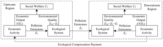
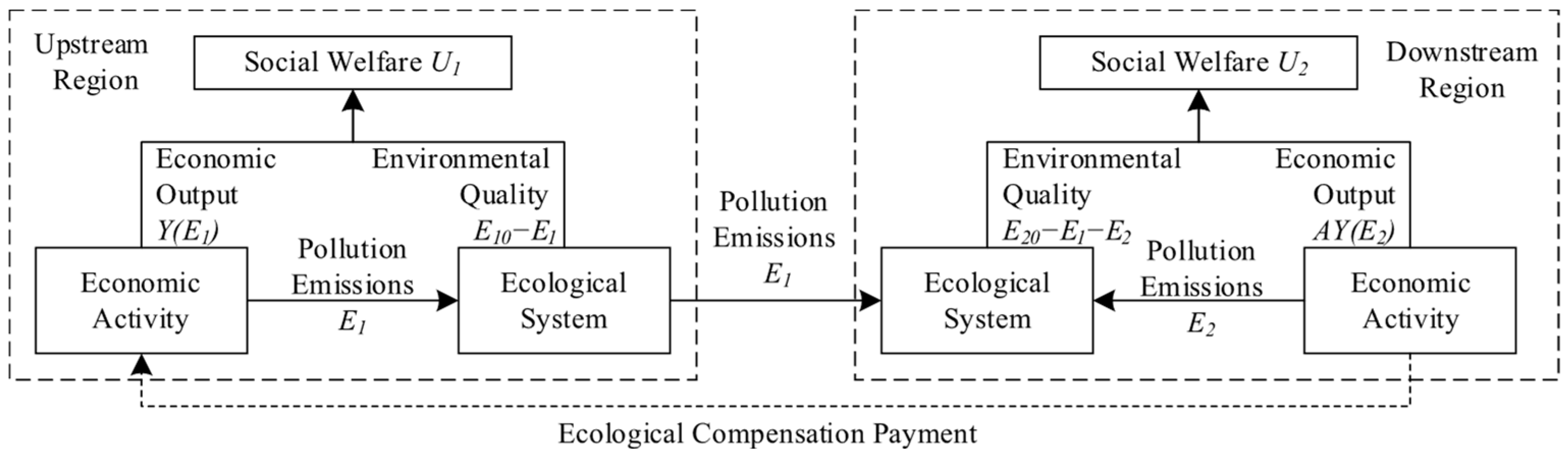
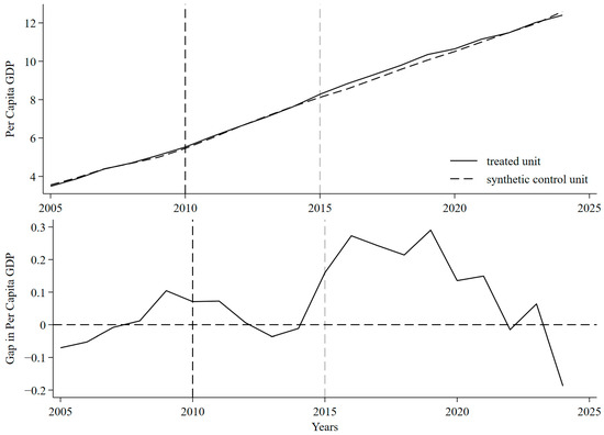
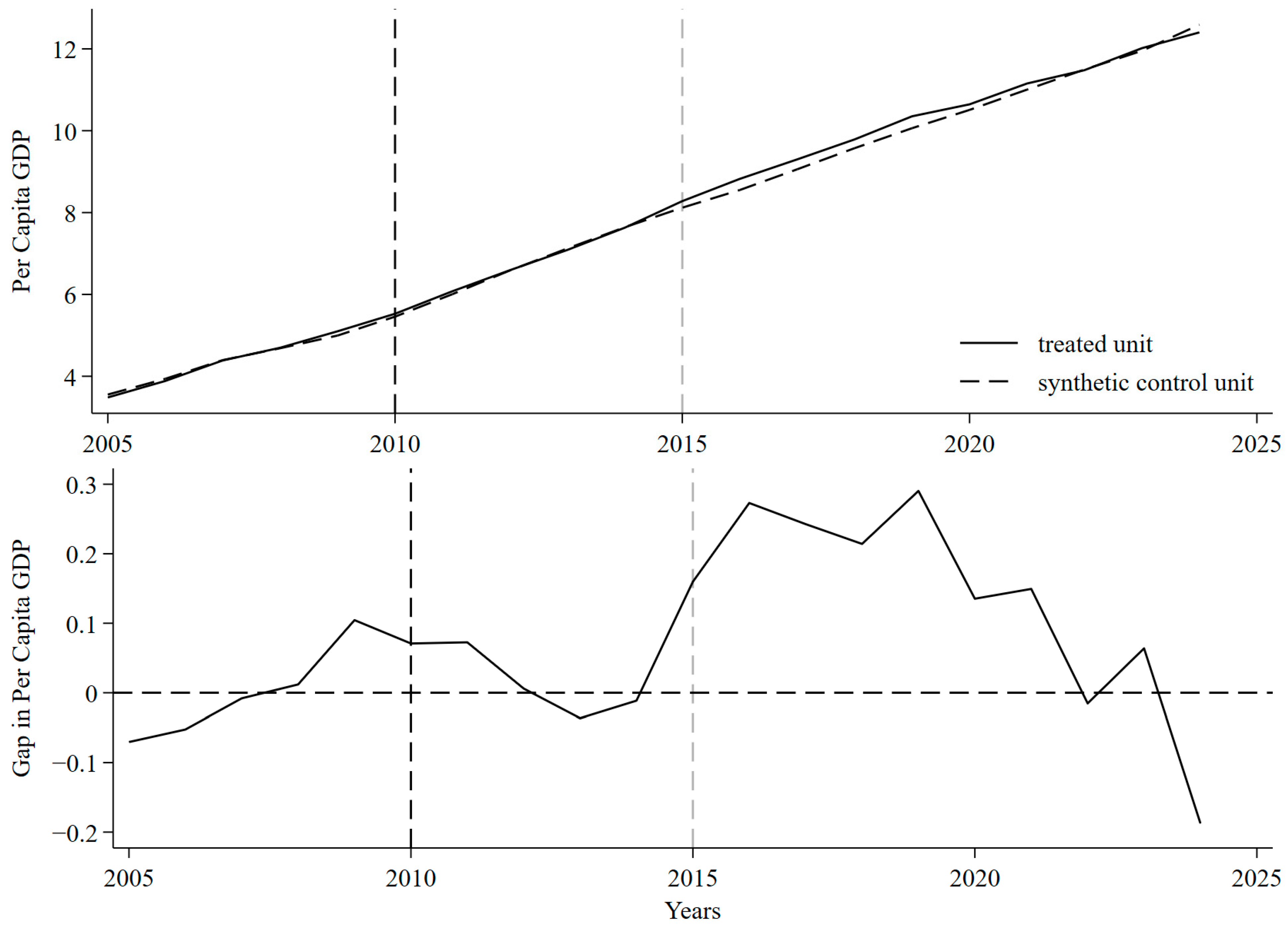
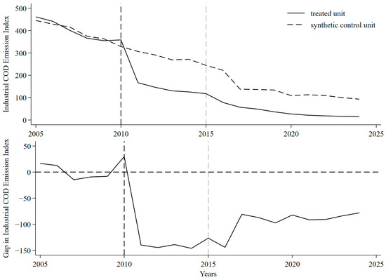
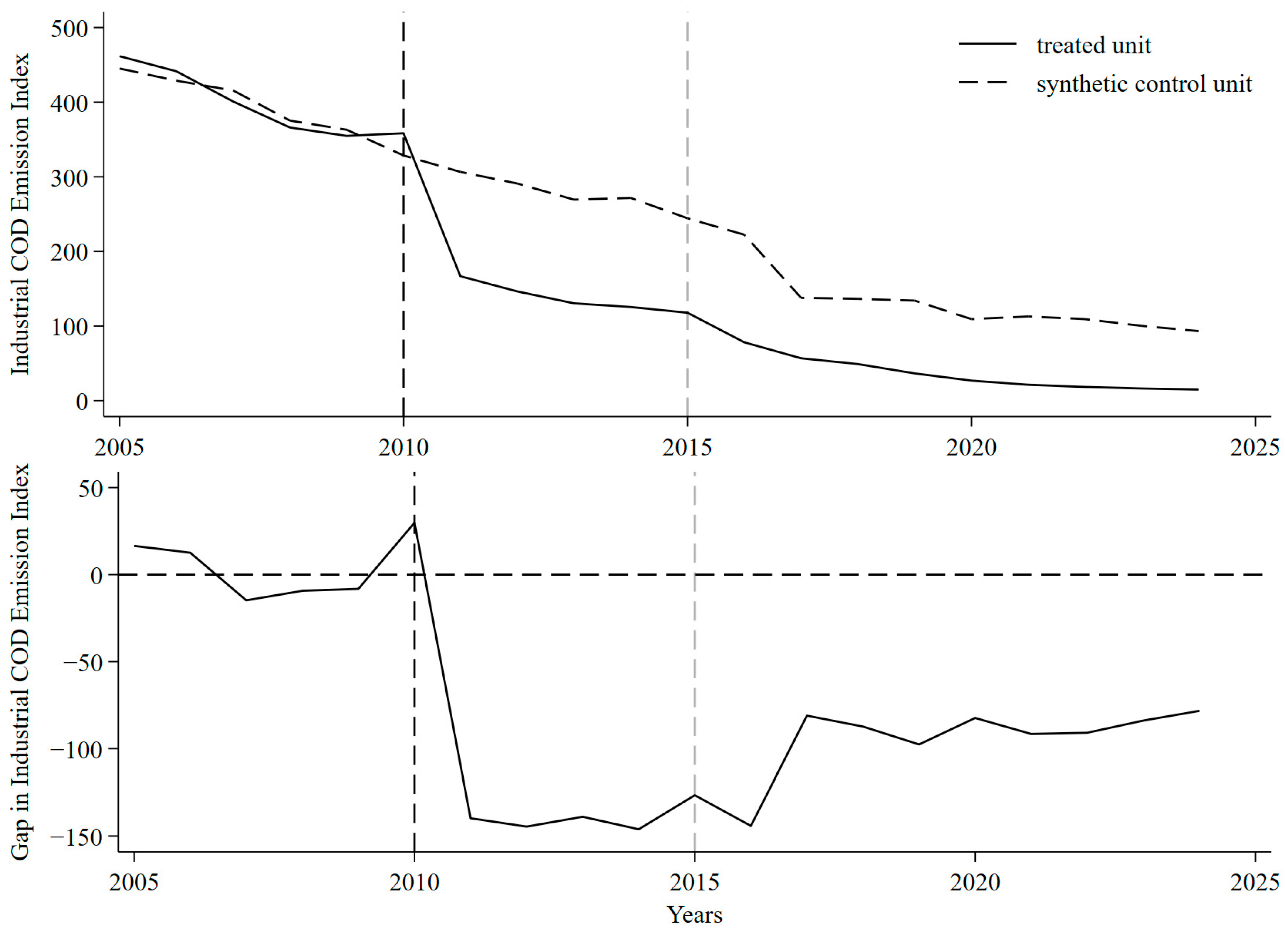
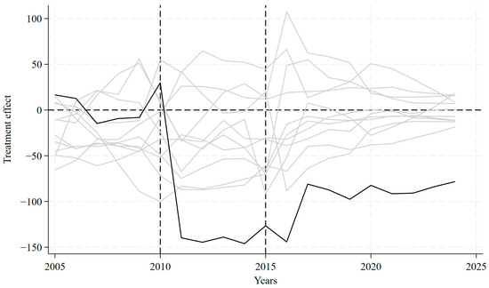
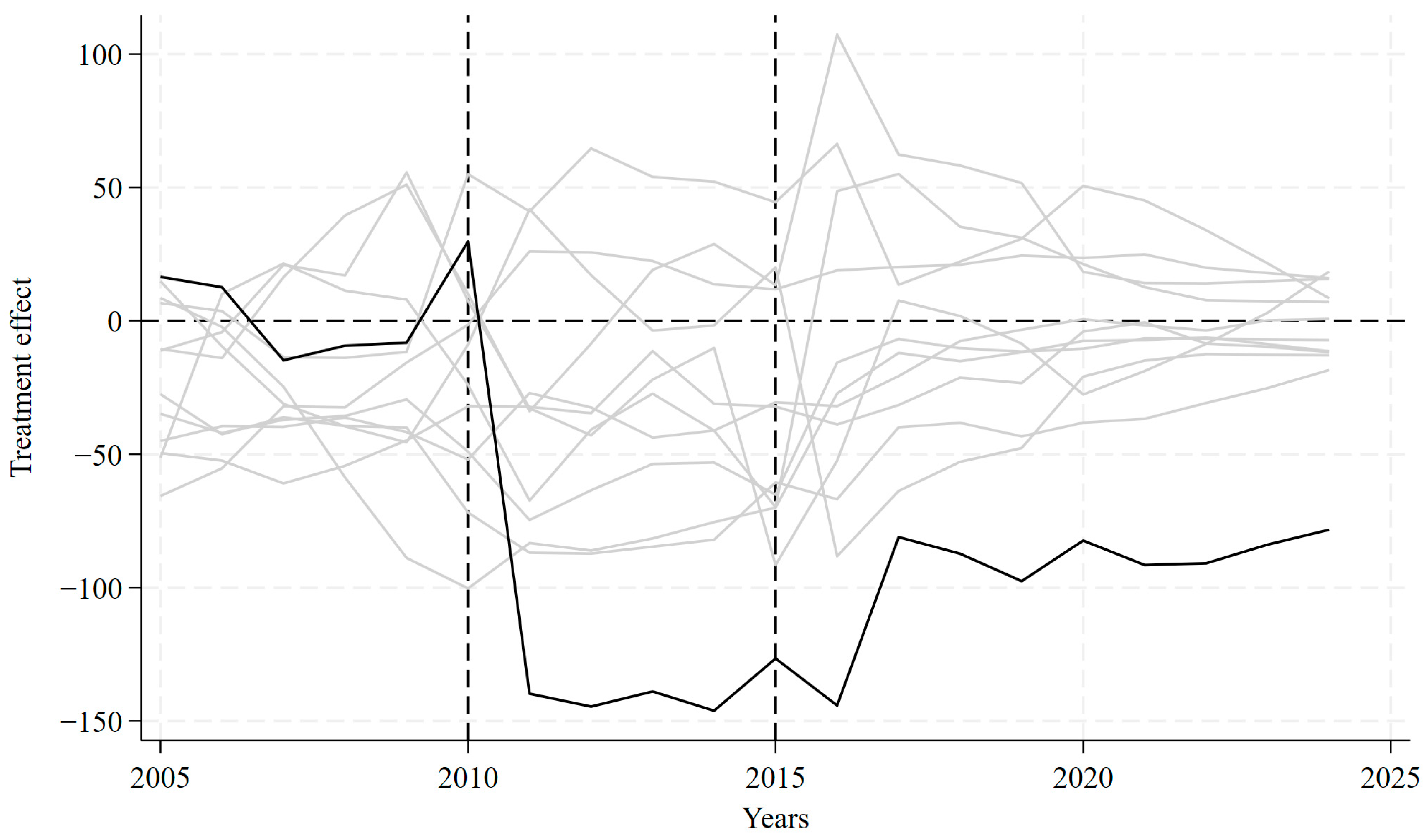
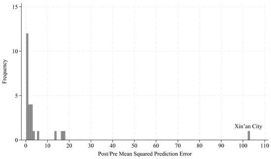
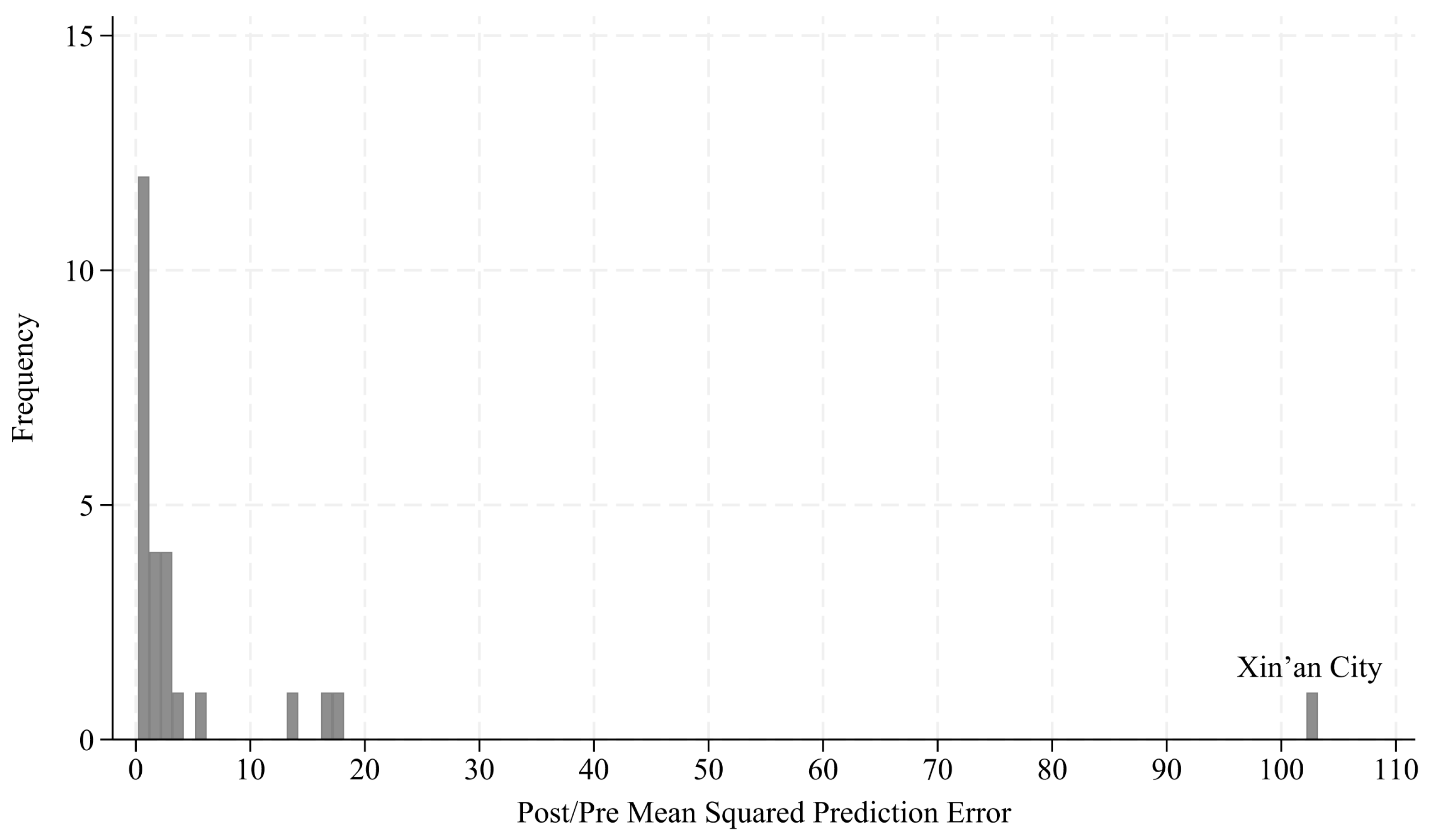
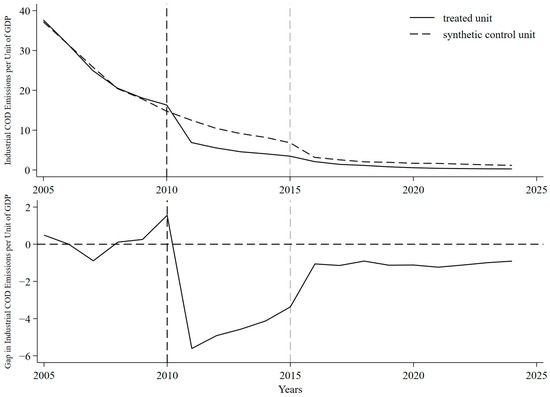
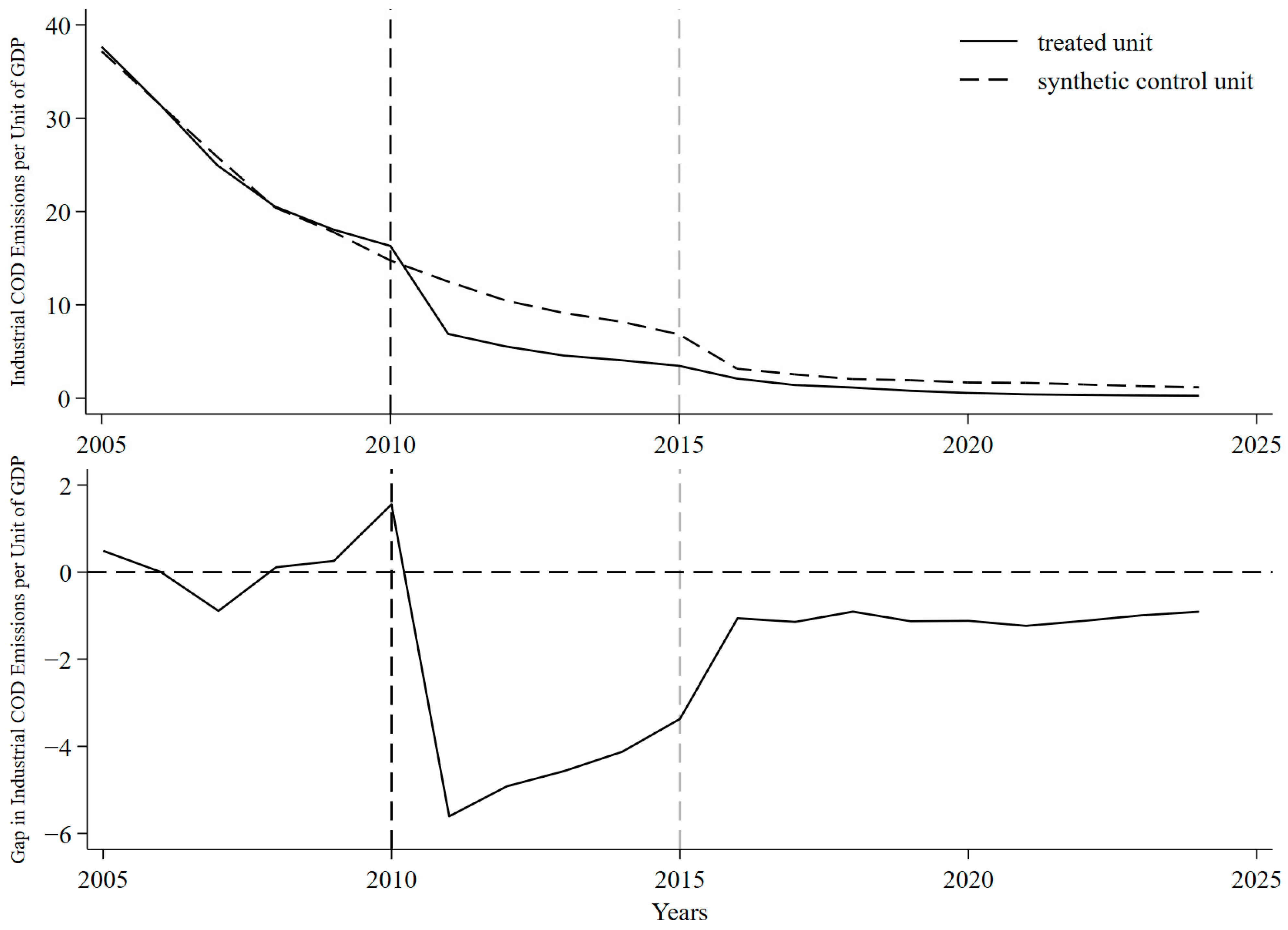
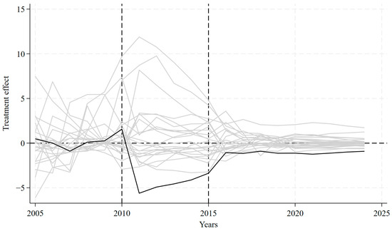
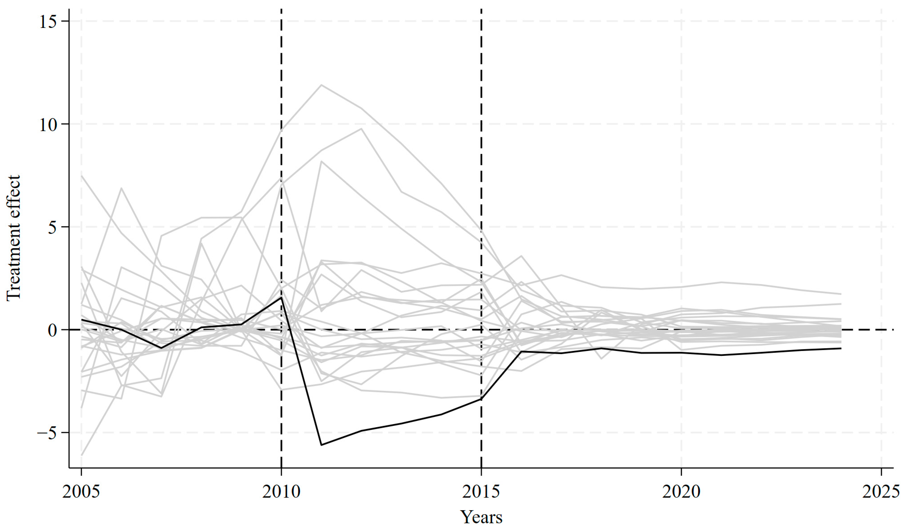
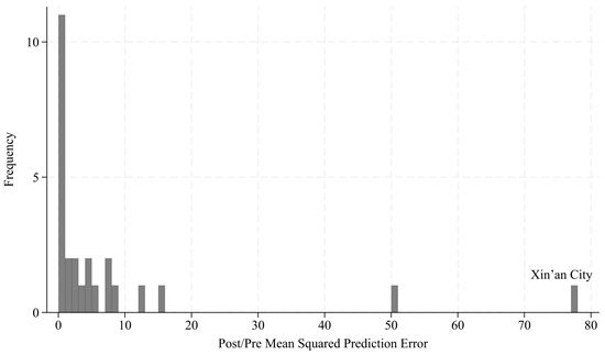
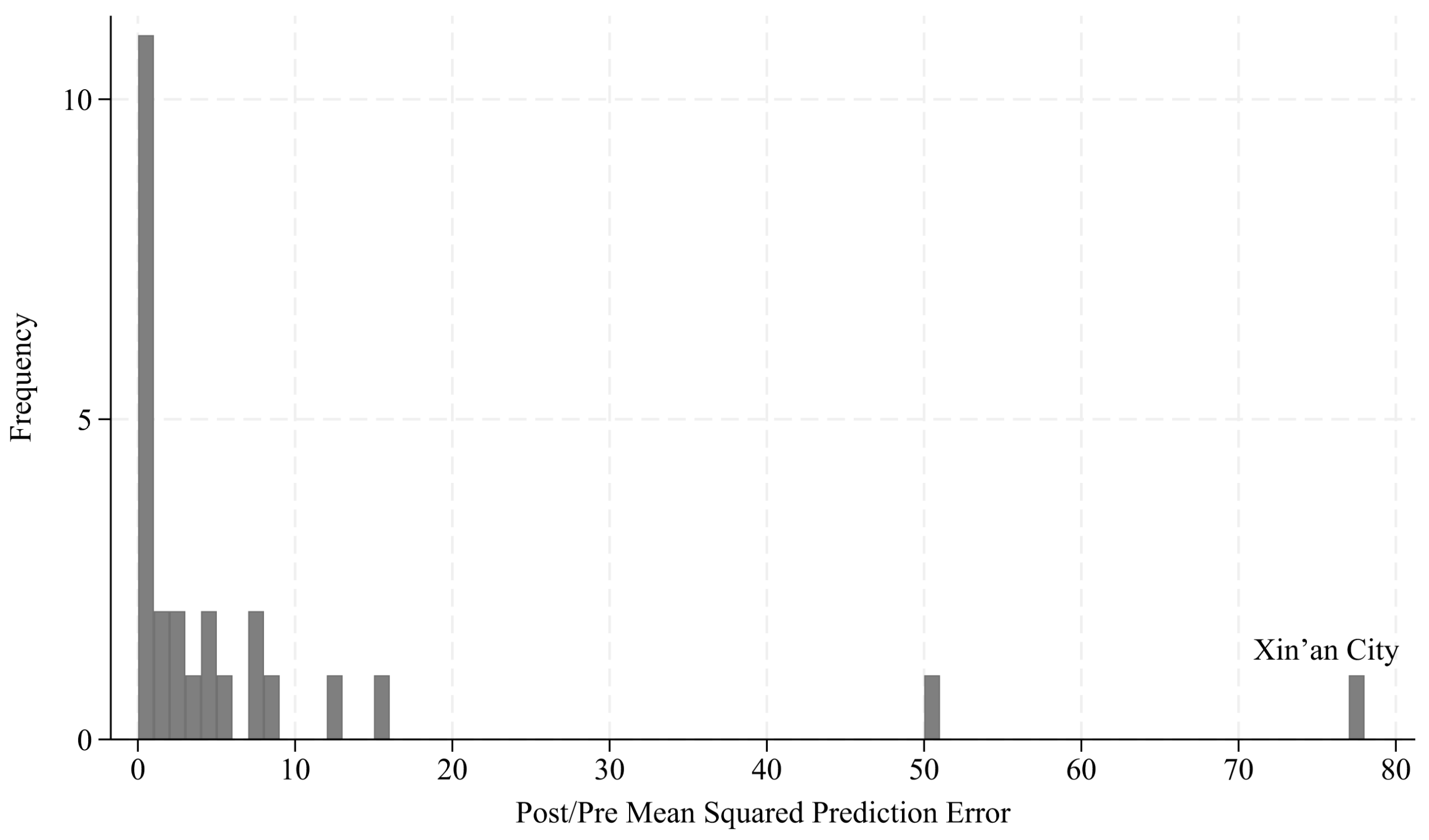

Disclaimer/Publisher’s Note: The statements, opinions and data contained in all publications are solely those of the individual author(s) and contributor(s) and not of MDPI and/or the editor(s). MDPI and/or the editor(s) disclaim responsibility for any injury to people or property resulting from any ideas, methods, instructions or products referred to in the content. |
© 2026 by the authors. Licensee MDPI, Basel, Switzerland. This article is an open access article distributed under the terms and conditions of the Creative Commons Attribution (CC BY) license.