Physics-Informed Neural Network for Reconstructing Free-Surface Transient Flow Fields in Long-Distance Water-Conveyance Tunnels from Sparse Observations

Abstract

Long-distance free-surface water-conveyance tunnels require a spatially continuous representation of transient water depth, yet in practice flow is monitored at only a few sections. This study develops a physics-informed neural network (PINN) that reconstructs the transient water-depth field of unsteady free-surface flow in such tunnels from two- or three-point sensors. The one-dimensional Saint-Venant equations, closed with a Darcy–Weisbach steady friction term in hydraulic-radius form, are embedded as a soft constraint in the training loss, so that sparse depth observations are combined with the governing conservation laws to recover the field at unobserved interior and downstream locations. High-resolution finite-volume (FVM) solutions of a 500 m circular tunnel under a flood-rise scenario provide the reference data. The PINN reduces the relative L₂ error at unobserved sections to approximately one-quarter of that of an otherwise identical, physics-free ANN (2.50% versus 10.05% at an interior section; 4.77% versus 13.69% at an extrapolation section). Runs repeated with different random seeds confirm statistical stability at zero noise, while revealing that a minority of trainings at 10% noise converge to spurious solutions. Sensor-placement experiments, including layouts anchored at the true domain boundaries (x = 0 and 500 m), show that boundary anchoring—particularly of the upstream boundary—governs both accuracy and noise robustness: boundary-anchored two-sensor layouts remain accurate in most runs under 10–20% observation noise, whereas interior-only layouts degrade sharply. The method is presented as an offline reconstruction tool; its extension to streaming data assimilation is discussed as future work.

1. Introduction

Long-distance water-conveyance systems transfer water over tens to hundreds of kilometers through open canals and low-pressure conveyance tunnels and provide important infrastructure for regional water security and inter-basin allocation. In these free-surface conduits, routine operations, including gate adjustment and inflow or demand regulation, continually induce unsteady flow, so that depth waves travel along the full reach before dissipating. A spatially continuous, time-resolved representation of water depth h (x, t) along the conduit is consequently important for conveyance safety, real-time scheduling and overtopping warning. In practice, however, flow is monitored at only a few gauging sections, and the complete spatiotemporal field must be inferred from sparse measurements. This problem is therefore an inverse data-assimilation problem: recovering a PDE-constrained field from point observations.

Classical approaches to this inverse problem are dominated by variational and adjoint-based data assimilation, in which a forward model is constrained to sparse observations by minimizing a cost functional using an adjoint model. For the shallow-water equations, this line of work dates back to Courtier and Talagrand’s variational assimilation with the direct and adjoint shallow-water equations [1], and has since become standard practice in operational meteorology and oceanography. These methods are theoretically elegant and statistically rigorous, but they require a differentiable forward solver and its adjoint, both of which are laborious to implement and maintain for free-surface flow in complex geometries and involve cost that grow steeply with the number of control variables. This motivates the exploration of mesh-free, adjoint-free alternatives, of which physics-informed neural networks are the most prominent.

Two established method classes are also used to characterize such flows, but each is limited under sparse field conditions. The first solves the Saint-Venant equations numerically, for example with the method-of-characteristics [2] or Godunov-type finite-volume schemes [3]. These forward solvers are physically rigorous and remain standard tools for design analysis, but they require specified boundary and initial conditions as well as well-calibrated hydraulic parameters, such as channel roughness and friction. Their accuracy deteriorates when an upstream or downstream boundary is unknown or when roughness changes as a conduit age, and they provide no natural means of assimilating the sparse, noisy monitoring data obtained during operation. The second class replaces the physics with data-driven models. Convolutional and long short-term memory (LSTM) networks, including hybrid models, have been used to predict streamflow and water level from historical records [4,5], including coupled water-level and water-quality prediction with CNN–LSTM [6]. Although these models are fast at inference, they lack physical interpretability, require large volumes of high-quality labeled data and extrapolate poorly beyond gauged locations. This limitation is particularly important for sparsely monitored conveyance lines, where most of the field is unobserved.

Physics-informed neural networks (PINNs) [7] provide an alternative that combines these two approaches and have become an established framework in scientific machine learning [8,9]. By embedding the residuals of governing partial differential equations as soft constraints in the loss function, a PINN combines observations with conservation laws in a mesh-free model. It can therefore operate with substantially less labeled data than a purely data-driven emulator and, in principle, infer the solution where no data are available. Domain-decomposition variants, such as the extended PINN (XPINN) [10], extend this framework to multiscale and multi-domain problems. In pressurized pipeline systems, PINNs have been developed most extensively for water-hammer transients as inverse data-assimilation tools. Waqar et al. [11] reconstructed transient-wave propagation in a reservoir–pipe–reservoir system. Ye et al. [12] trained a PINN with method-of-characteristics data and validated it experimentally for a single pipe, before extending the approach to reconstruct transient pressures in pipe networks from local observations [13]. Zhang and Shafieezadeh [14] introduced adaptive loss weighting for natural gas pipeline transients, and Yan et al. [15] embedded nodal mechanistic information directly in the loss to train a unified hybrid model for water-distribution networks. This literature shows that PINNs can assimilate sparse sensor data and infer unobserved states in closed-conduit water hammer, but not for free-surface flow.

PINNs have also been used to solve the Saint-Venant and shallow-water equations for free-surface and open-channel flows. Cheng and Zhang [16] combined a PINN with residual blocks for fluid-flow problems governed by these equations. Feng et al. [17] used a Saint-Venant PINN to downscale a large-scale river model, Niu et al. [18] solved coupled one-dimensional surface-flow and transport equations, and Qi et al. [19] solved two-dimensional shallow-water equations for inundation without labeled data. PINNs have also been applied to related tunnel-engineering problems, including deep-tunnel seepage-field prediction [20]. Inverse parameter-identification formulations for free-surface systems are beginning to emerge, for example, including spatially distributed parameter identification for the two-dimensional shallow-water equations [21]. However, most free-surface PINN studies remain forward solvers or downscaling schemes with prescribed boundary and initial conditions. Inverse reconstruction of a complete transient field from a few sparse, potentially boundary-deficient observations has not been established for long-distance free-surface transients, although this capability is now common in pressurized water-hammer applications.

Tunnel engineering increasingly relies on the fusion of monitored data with physical or knowledge-based models. In tunnel support-safety assessment, Lai et al. [22] proposed a data- and knowledge-dual-driven framework combining machine learning with ex-pert-knowledge weighting, and in sub-sea tunnel lining design, Zhao et al. [23] combined numerical simulation of lining water pressure with field measurements to calibrate a pressure-reduction coefficient. These studies illustrate the value of dual-driven monitoring frameworks for tunnel safety assessment: reconstructed hydraulic states, such as the water-depth field targeted here, are the natural input to such water-pressure and safety assessments. This study differs from them in that it targets the free-surface transient flow field itself—the hydraulic state—rather than geotechnical support behavior, and reconstructs this state from sparse hydraulic sensors under a hyperbolic PDE constraint.

Two gaps therefore remain. First, PINN reconstruction of hydraulic transients is concentrated in pressurized systems, whereas free-surface PINN studies predominantly solve forward problems. Inverse reconstruction of free-surface transients from sparse observations remains largely unexplored. Second, when reconstruction relies on only a few point sensors, the layouts that render the inverse problem sufficiently well posed and robust to measurement noise are not known. Optimal sensor placement has been studied extensively in water-distribution networks, commonly for leak localization or contamination detection using evolutionary or graph-based optimization [24]. However, it has not been examined as a factor governing the well-posedness of PINN field reconstruction. Existing reconstruction studies generally treat sparse-sensor placement as a fixed experimental setting rather than a design variable, even though it may control attainable accuracy in a boundary-driven hyperbolic system. Accordingly, both sparse reconstruction of long-distance free-surface transients and the placement principles needed to make that reconstruction reliable remain open problems.

To address these gaps, this study develops a Saint-Venant-constrained PINN for inverse reconstruction of free-surface transient flow fields in long-distance conveyance tunnels from sparse observations. The reconstruction method is the central contribution. First, the PINN embeds the one-dimensional Saint-Venant equations as a soft constraint and reconstructs the water-depth field from only two- or three-point sensors under boundary-deficient conditions. This is an inverse data-assimilation problem rather than the forward solution considered in most free-surface PINN studies. Second, a controlled physics ablation, in which the same network is trained with and without the physical constraint, isolates the contribution of physics at interpolation and extrapolation locations; additional ablations of the initial-condition term and of the friction closure quantify the role of each loss component. Third, sensitivity analyses of network depth, loss weights and training budget establish a stable configuration and show that the method does not require case-specific tuning, and the statistical stability of the main conclusions at zero noise is verified by repeated runs with different random seeds, which also reveal a spurious-solution failure mode at 10% noise (Section 3.3.3). Finally, sparse-sensor placement is treated as a design variable. Three- and two-sensor layouts are classified by spatial topology and evaluated with injected-noise tests, complemented by layouts anchored at the true domain boundaries, yielding a transferable placement principle and a characterization of noise robustness for monitoring-network design. Finally, the generality of the reconstruction is tested on independent scenarios with different boundary perturbations, friction and geometry, and the reliability of the reference solution is established through grid-refinement, conservation and cross-method (MOC) checks. Section 2 describes the methodology, Section 3 presents the results and discussion, and Section 4 gives the conclusions.

2. Materials and Methods

2.1. Study System and Reference-Data Generation

The test system is a single long-distance free-surface conveyance tunnel subject to an upstream boundary disturbance. In a physical experiment, pressure and level sensors cannot be deployed densely enough to sample the flow field throughout the tunnel; a validated, high-resolution forward model of the same system is therefore used as the source of training observations and evaluation data, exactly as in related PINN validation studies for pressurized pipelines [12].

The reference solution is generated with a one-dimensional Godunov-type finite-volume solver for the Saint-Venant equations of Section 2.2. The conduit is divided into N = 500 finite-volume cells. Mass and momentum fluxes at cell interfaces are evaluated with an HLL approximate Riemann solver [25], and second-order spatial accuracy is obtained using MUSCL reconstruction [26] with a Minmod slope limiter to suppress spurious oscillations near steep gradients [27]. Bed-slope and friction source terms are treated with a standard explicit source-term formulation, and the solution is advanced with an adaptive time step satisfying the Courant–Friedrichs–Lewy stability condition [28]. The scheme conserves mass and momentum discretely; a dedicated check of the full-resolution solution showed that the residual of the discrete mass balance dV/dt − Q_in vanishes to within 1.1% of the RMS inlet flux (Section 3.5.1). Because the present case is fully wetted at all times (h ≥ 2.0 m throughout the domain, with a maximum depth of 7.7 m against a diameter of 8.0 m), no wet–dry fronts arise and positivity of the water depth is preserved by the HLL–MUSCL update, with the depth clamped to the geometric range of the circular section. Well-balanced and positivity-preserving treatments of the Saint-Venant system for non-homogeneous domains, as discussed by Li et al. [29], are therefore not required here but would become relevant for dry-bed or steep-topography cases. Grid convergence of the reference solution is verified in Section 3.5.1: the monitoring-section series obtained with N = 250, 500 and 1000 cells converge monotonically, with a relative L₂ difference of 0.81% between the N = 500 and N = 1000 solutions, indicating that N = 500 adequately resolves the transient. An independent first-order method-of-characteristics (MOC) implementation of the same initial-boundary-value problem, also with Darcy–Weisbach friction, was used as a cross-method check of the reference solution (Section 3.5).

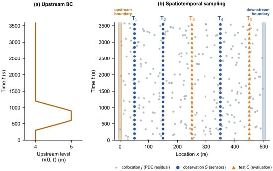
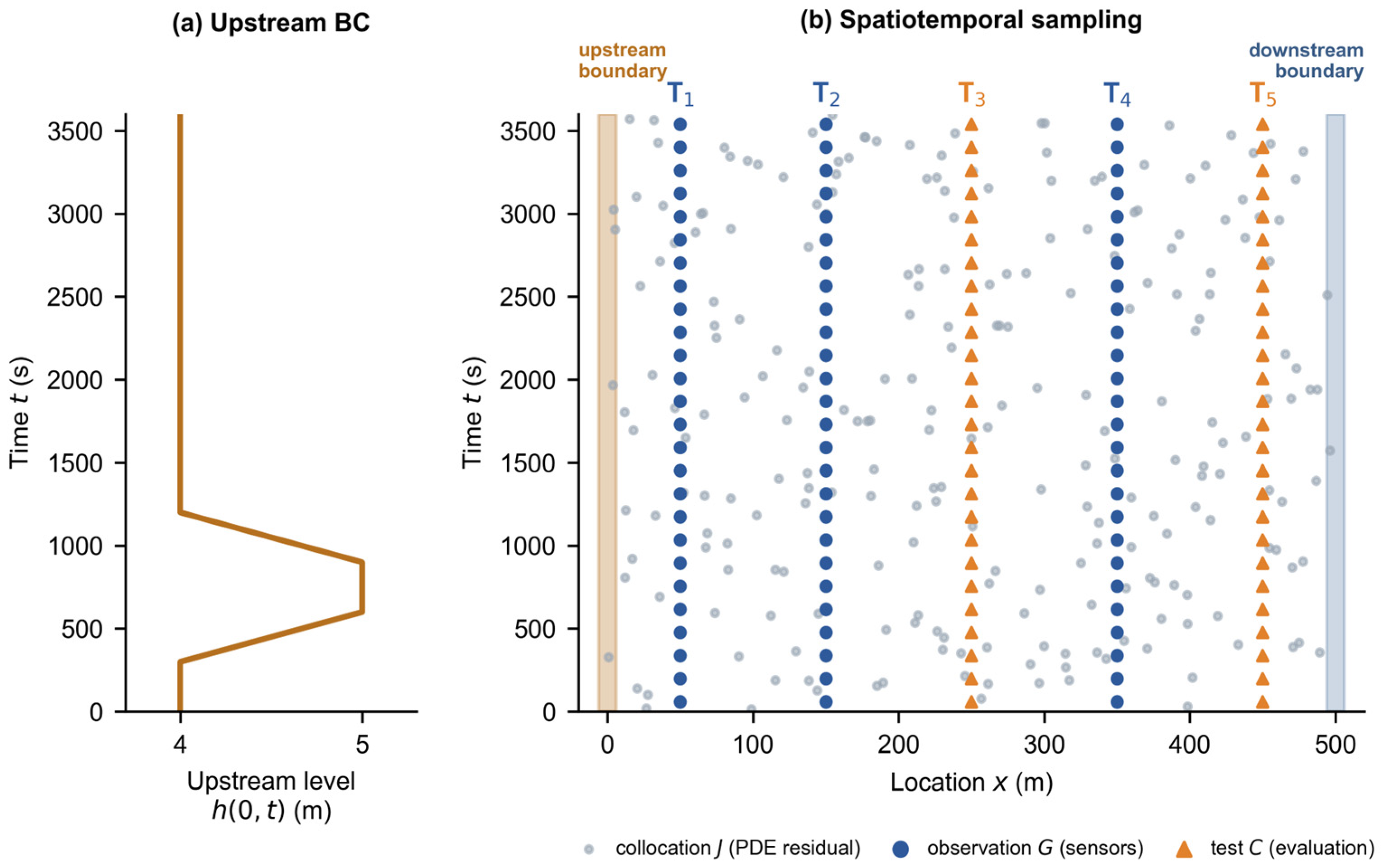
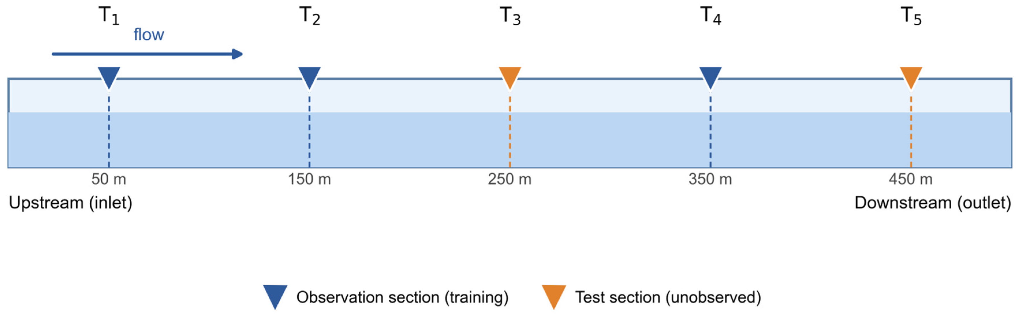
The conduit has a circular cross-section with length L = 500 m, diameter D = 8.0 m, bed slope S₀ = 0.0005, Darcy–Weisbach friction factor f = 0.012 and gravitational acceleration g = 9.81 m s⁻². The initial state is hydrostatic rest: a uniform water depth h (x, 0) = 2.0 m and zero discharge Q (x, 0) = 0 throughout the tunnel. The upstream boundary condition is a prescribed water-level hydrograph at the inlet (Figure 1a): the inlet level equals the initial depth of 2.0 m at t = 0 and is raised rapidly to 4.0 m at the start of the simulation—representing the opening of an upstream reservoir or gate—then rises linearly from 4.0 to 5.0 m during t = 300–600 s (a flood-rise phase), remains at 5.0 m for 300 s, and falls linearly back to 4.0 m during t = 900–1200 s. The downstream end is a closed blind end (wall boundary condition, Q = 0), which reflects waves back into the tunnel and is representative of the terminal section of a conveyance tunnel. The resulting flow is subcritical throughout: the Froude number computed from the reference solution never exceeds 0.81, with a mean of 0.12. Five candidate monitoring sections, T₁–T₅, are located at x = 50, 150, 250, 350 and 450 m. Water depth h is the primary dependent variable throughout; the reference series used for training and evaluation are the depth series at these sections, and only depth is observed in all experiments of this study (Section 2.4).

Figure 1. (a) Upstream boundary condition: the prescribed inlet water level h(0, t) follows a flood-rise hydrograph (4.0 → 5.0 → 4.0 m). (b) Spatiotemporal sampling in the x–t domain. Collocation points J (gray) impose the PDE residual over the whole domain; observation points G (blue) supply the sparse measured depth series at the sensor sections T₁–T₅; test points C (orange) at other sections are used only for evaluation. The upstream (x = 0) and downstream (x = 500 m) boundaries are highlighted.

2.2. Governing Equations

Unsteady free-surface flow in the conduit is described by the one-dimensional Saint-Venant equations [30,31], which express conservation of mass and momentum:

$${\displaystyle \frac{\partial A}{\partial t}}+{\displaystyle \frac{\partial Q}{\partial x}}=0$$

(1)

$${\displaystyle \frac{\partial Q}{\partial t}}+{\displaystyle \frac{\partial }{\partial x}}\left({\displaystyle \frac{Q^2}{A}}\right)+gA\hspace{0.17em}{\displaystyle \frac{\partial h}{\partial x}}=gA\hspace{0.17em}\left(S_0-S_f\right)$$

(2)

where A is the wetted cross-sectional area (m²), Q is discharge (m³ s⁻¹), h is water depth (m), g is gravitational acceleration (m s⁻²), S₀ is bed slope (dimensionless) and S_f is friction slope (dimensionless). The equations are expressed in terms of discharge Q and no lateral inflow is considered. For a circular cross-section of diameter D, the wetted area A and free-surface top width B are defined exactly as functions of depth h through the wetted central angle θ:

$$\theta =2\mathrm{a}\mathrm{r}\mathrm{c}\mathrm{c}\mathrm{o}\mathrm{s}\left(1-{\displaystyle \frac{2h}{D}}\right)$$

(3)

$$A={\displaystyle \frac{D^2}{8}}\left(\theta -\mathrm{s}\mathrm{i}\mathrm{n}\theta \right)$$

(4)

$$B=D\hspace{0.17em}\mathrm{s}\mathrm{i}\mathrm{n}{\displaystyle \frac{\theta }{2}}$$

(5)

which hold for 0 ≤ h ≤ D and enter the residuals of Section 2.3 through automatic differentiation. The hydraulic radius is R = A/P_w, where $P_w=D{\displaystyle \frac{\theta }{2}}$ is the wetted perimeter.

The friction slope is represented by the Darcy–Weisbach steady-friction law written in hydraulic-radius form, which is the standard closure for gradually varied and slowly varying transient open-channel flow and is exactly the closure used in the reference finite-volume solver:

$$S_f={\displaystyle \frac{fQ\left|Q\right|}{8gR\hspace{0.17em}{A}^2}}$$

(6)

where f = 0.012 is the Darcy–Weisbach friction factor (dimensionless) and R is the hydraulic radius (m). Equation (6) is dimensionally consistent: with [Q] = m³ s⁻¹, [R] = m and [A] = m², the right-hand side is dimensionless. For steady uniform flow, Equation (6) reduces to the familiar S_f = f u²/(8gR) with u = Q/A.

The choice of a steady friction closure, and the role of unsteady (Brunone-type) friction in free-surface flow, deserve explicit discussion. Brunone’s instantaneous-acceleration friction model was originally developed for pressurized-pipe water hammer [32,33], in which the unsteady wall shear depends on the local and convective accelerations; extensions of acceleration-based friction to Saint-Venant (mixed-flow) modeling exist [34], and the calibration of such models in open channels remains an open research question [35]. For free-surface flow, the natural adaptation re-places the pipe wave speed a by the free-surface wave celerity $c= \sqrt{gA/B}$ and the pipe diameter by the hydraulic radius R, giving

$$S_f={\displaystyle \frac{k_b}{gA}}\left({\displaystyle \frac{\partial Q}{\partial t}}+c\hspace{0.17em}\mathrm{s}\mathrm{g}\mathrm{n}(Q)\left|{\displaystyle \frac{\partial Q}{\partial x}}\right|\right)$$

(7)

where k_b is a dimensionless Brunone-type coefficient. In this study, the momentum balance is dominated by the pressure, convective and local-inertia terms, and both the Darcy term and a Brunone-type term with typical pressurized-pipe coefficients (k_b = 0.03–0.05) are an order of magnitude smaller (Section 3.5.1); moreover, no calibrated value of k_b exists for open-channel flow. A steady Darcy–Weisbach closure was therefore retained throughout, and an ablation with the Brunone-type term included in the PINN residual confirms that it does not materially change the reconstruction (Section 3.5). We emphasize that this does not imply that unsteady friction is negligible in general free-surface transients—for fast surge fronts or mixed-flow transitions, it may be required—but that the present flood-rise scenario is sufficiently slowly varying for the steady closure to be adequate, as quantified in Section 3.5.

2.3. PINN Architecture

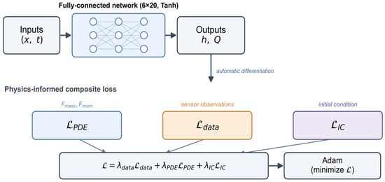
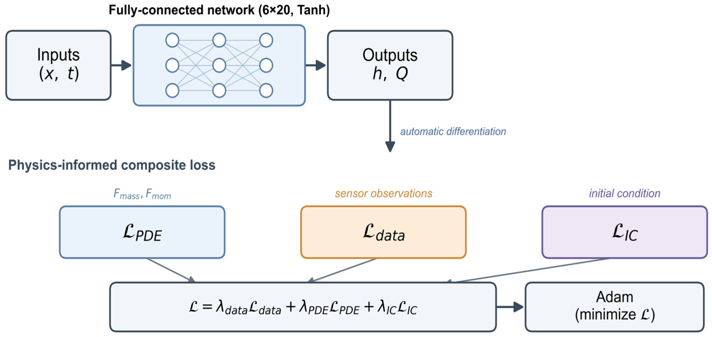
The solution is approximated by a fully connected feed-forward neural network that maps space–time coordinates to the flow state. The input layer contains two neurons, representing spatial coordinate x and time t. The output layer contains two neurons, representing the Saint-Venant variables water depth h(x, t) and discharge Q(x, t). The network architecture is shown in Figure 2. Both enter the physical residuals defined below; this study reports water-depth reconstruction as the primary result, while retaining Q as an auxiliary output. Hidden layers use the hyperbolic-tangent (Tanh) activation function, whose differentiability supports the derivatives required by the PDE residual. To reduce the effect of dimensional disparity during gradient descent, the inputs are normalized to the interval [−1, 1]:

$$\widehat{x}=2\hspace{0.17em}{\displaystyle \frac{x-x_{\mathrm{m}\mathrm{i}\mathrm{n}}}{x_{\mathrm{m}\mathrm{a}\mathrm{x}}-x_{\mathrm{m}\mathrm{i}\mathrm{n}}}}-1$$

(8)

$$\widehat{t}=2\hspace{0.17em}{\displaystyle \frac{t-t_{\mathrm{m}\mathrm{i}\mathrm{n}}}{t_{\mathrm{m}\mathrm{a}\mathrm{x}}-t_{\mathrm{m}\mathrm{i}\mathrm{n}}}}-1$$

(9)

Figure 2. Architecture of the Saint-Venant-constrained PINN. A fully-connected network maps the space–time coordinates (x, t) to the water depth h and discharge Q; the composite loss combines the PDE-residual term (from automatic differentiation of the Saint-Venant equations), the sparse-sensor data term, and the initial-condition term, and is minimized by Adam.

Unlike a purely data-driven model, the PINN obtains derivatives of its outputs with respect to the input coordinates directly by automatic differentiation, without mesh discretization [7]. Substitution of these derivatives into the governing equations gives the mass and momentum residuals,

$$F_{\mathrm{mass}}={\displaystyle \frac{\partial A}{\partial t}}+{\displaystyle \frac{\partial Q}{\partial x}}$$

(10)

$$F_{\mathrm{mom}}={\displaystyle \frac{\partial Q}{\partial t}}+{\displaystyle \frac{\partial }{\partial x}}\left({\displaystyle \frac{Q^2}{A}}\right)+gA\hspace{0.17em}{\displaystyle \frac{\partial h}{\partial x}}-gA\hspace{0.17em}\left(S_0-S_f\right)$$

(11)

where ${\displaystyle \frac{\partial A}{\partial t}}=B{\displaystyle \frac{\partial h}{\partial t}}$ has been used, which are driven toward zero during training so that the network predictions satisfy the physical conservation laws.

2.4. Spatiotemporal Sampling

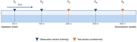
Following common PINN practice [7,36], the training data are organized into three types of space–time points, each serving a distinct role in coupling observations with the physical constraint. The five candidate monitoring sections T1–T5 supply the observation and test series (Figure 3). With the simulation time discretized into N_t instants, the three sets illustrated in Figure 1 are with i = 1, …, N_t for the observation and test sets. The observed depth $h(x_g, t_i)$ is known only on the observation set $\mathcal{G}$, the PDE residuals are evaluated on the collocation set $\mathcal{J}$, which is resampled randomly at every iteration and is therefore not restricted to a fixed set of sections; and the test set $\mathcal{C}$ is disjoint from $\mathcal{G}$ and is used only for evaluation. Throughout this study, only water depth h is observed; the discharge Q is never supplied to the network and is constrained solely by the momentum residual and the initial condition.

$$\mathcal{G}={\left\{\left(x_g,t_i\right)\right\}}_{g=1,\dots ,N_G}, \mathcal{J}=\left\{\left(x_j,t_i\right)\right\}, \mathcal{C}={\left\{\left(x_c,t_i\right)\right\}}_{c=1,\dots ,N_C}$$

(12)

Figure 3. Layout of the five candidate monitoring sections T₁–T₅ along the 500 m conduit. In the validation study (Section 3.1), T₁, T₂ and T₄ are observation (training) sections, and T₃ and T₅ are unobserved test sections.

Observation points (G) are space–time samples at the sensor sections. At these points, numerically generated depth series are supplied to the network, forming the observation set used in the data-fidelity term; these are the only points at which measured values are used. The observation points lie on the vertical lines $x = x_G$ at the sensor sections and span the full simulation period.

Collocation, or residual, points (J) are space–time locations at which the PDE residuals F_mass and F_mom are evaluated to impose the governing equations. They carry no observed values. Instead, they sample the interior of the space–time domain so that the physical constraint is imposed throughout the field, including regions between and beyond the sensors. Because these points are resampled at every training iteration (Section 2.5), the constraint is distributed across the domain rather than concentrated near the observations.

Test points (C) are located at sections other than the observation sections and are withheld from training. They are used only to evaluate reconstruction performance. As they lie away from observed sections, they test both interpolation within the envelope of the observation sections and extrapolation outside it.

2.5. Composite Loss Function and Training

The network parameters are optimized by minimizing a composite loss that linearly combines an observation-data loss, a PDE-residual loss, and an initial-condition loss:

$${\mathcal{L}}_{\mathrm{total}}={\lambda }_{\mathrm{data}}\hspace{0.17em}{\mathcal{L}}_{\mathrm{data}}+{\lambda }_{\mathrm{PDE}}\hspace{0.17em}{\mathcal{L}}_{\mathrm{PDE}}+{\lambda }_{\mathrm{IC}}\hspace{0.17em}{\mathcal{L}}_{\mathrm{IC}}$$

(13)

where ${\mathcal{L}}_{\mathrm{data}}$ is the mean-squared error (MSE) between predicted and observed depths at the sparse observation points, ${\mathcal{L}}_{\mathrm{PDE}}$ is the mean squared residual of F_mass and F_mom over the collocation points, and ${\mathcal{L}}_{\mathrm{IC}}$ enforces the prescribed initial state (h = 2.0 m, Q = 0) at t = 0. The weights ${\lambda }_{\mathrm{data}}$, ${\lambda }_{\mathrm{PDE}}$ and ${\lambda }_{\mathrm{IC}}$ balance the gradient contributions of the three terms. Network parameters are updated with the Adam optimizer [37] using an initial learning rate of 1 × 10⁻³ and Xavier-normal initialization to reduce vanishing gradients and accelerate convergence. At each iteration, 2048 collocation points are randomly resampled from the space–time domain so that the physical constraint covers the entire field. Training involves stochastic resampling of collocation points; the resulting run-to-run variability is quantified in Section 3.3.3 by repeating representative trainings with different random seeds.

2.6. Accuracy Metric

Reconstruction accuracy is evaluated using the relative L₂ error:

$${\mathit{E}}_{{\mathit{L}}_{\mathbf{2}}}=\sqrt{{\displaystyle \frac{{\displaystyle {\sum }_{\mathit{i}=\mathbf{1}}^{\mathit{N}}}{\left({\mathit{u}}_{\mathrm{pred},\mathit{i}}-{\mathit{u}}_{\mathrm{true},\mathit{i}}\right)}^{\mathbf{2}}}{{\displaystyle {\sum }_{\mathit{i}=\mathbf{1}}^{\mathit{N}}}\hspace{0.17em}{\mathit{u}}_{\mathrm{true},\mathit{i}}^{\mathbf{2}}}}}$$

(14)

where ${\mathit{u}}_{\mathrm{pred}}$ and ${\mathit{u}}_{\mathrm{true}}$ are the predicted and reference vectors over N test points, respectively. The metric is dimensionless and therefore comparable across sections and scenarios. It aggregates deviations over the full time series rather than at isolated instants, representing the global energy difference between prediction and reference. Because it is based on the Euclidean norm, it is also sensitive to the local errors at surge peaks and troughs that the reconstruction must capture. To complement this global metric, Section 3.1 additionally reports peak-amplitude and phase-lag errors and the mass/momentum residuals of the reconstructed field, which address the accuracy of wave timing and of the underlying conservation laws, respectively.

3. Results and Discussion

3.1. Validation: PINN Versus Data-Driven ANN Under Sparse Observation

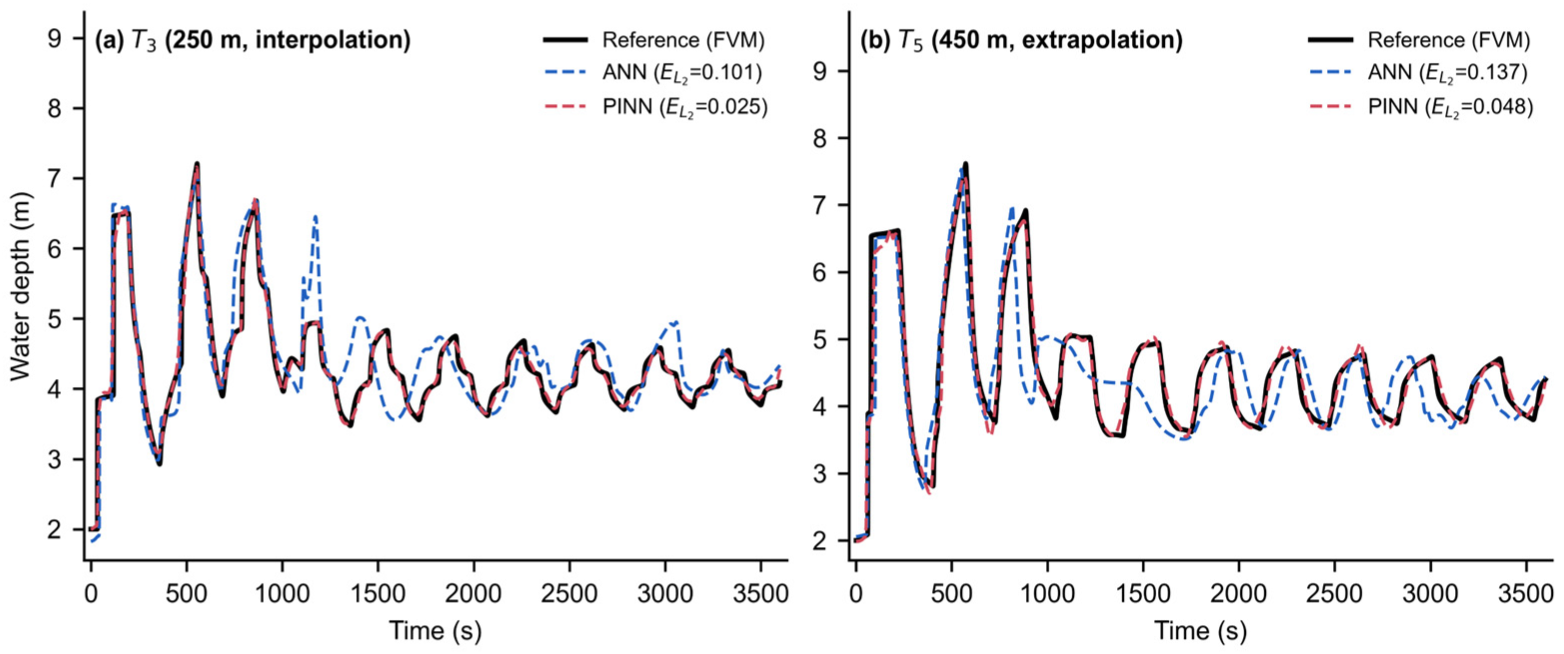
To determine whether the embedded physical mechanism is necessary under sparse observation, a purely data-driven ANN with an identical architecture and training configuration was used as the baseline. The ANN differs from the PINN only in the removal of the PDE-residual and initial-condition loss terms. The comparison is therefore a controlled physics ablation, not a benchmark against state-of-the-art data-driven predictors. Both networks had eight hidden layers with twenty neurons, Tanh activation and 500,000 iterations. They were trained on depth series at T₁ (x = 50 m), T₂ (x = 150 m) and T₄ (x = 350 m), and evaluated at T₃ (x = 250 m) and T₅ (x = 450 m). The PDE-loss and initial-condition weights of the PINN were 0.05 and 0.1, respectively. T₃ lies within the envelope of the observation sections and is therefore an interpolation point; T₅ lies outside it and is an extrapolation point.

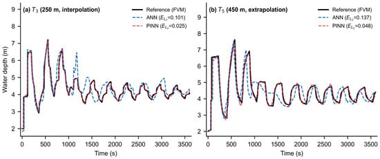
Table 1 reports the relative L₂ errors. The ANN error is several times larger than the PINN error at both sections and exceeds an engineering-acceptable range, whereas the PINN error remains low. Figure 4 illustrates the difference in waveform reconstruction. At interpolation section T₃, the ANN overshoots the fourth surge peak, advances the phase of the fourth and fifth peaks and, from approximately the eighth oscillation cycle, produces a spurious peak that exceeds all peaks in the true post-disturbance signal while lagging it in time. Several intervening troughs are similarly displaced. The deterioration is more severe at extrapolation section T₅: between the third and sixth cycles, the ANN prediction largely loses its peak-trough structure and subsequently drifts. This behavior is consistent with the nature of the model. The ANN is a high-dimensional nonlinear interpolator trained solely on statistical associations among observed series. In unobserved regions, where flow remains governed by the hyperbolic Saint-Venant system with defined propagation characteristics, it can produce only smooth or random curves that lack physical meaning. It cannot resolve the surge wave passing through the unobserved section, and its predictions therefore violate mass and momentum conservation. By contrast, the Saint-Venant-constrained PINN reproduces the magnitude and timing of surge waves throughout the 3600 s simulation.

Table 1. Relative L₂ errors of the ANN and the PINN at the test sections (error metric of Equation (14), with N equal to the number of time instants in the 3600 s series).

Location	ANN L2 Error	PINN L2 Error
T3 (x = 250 m, interpolation)	0.10054	0.025011
T5 (x = 450 m, extrapolation)	0.13688	0.047669

Figure 4. Predicted and reference water-depth series at (a) T₃ (x = 250 m, interpolation) and (b) T₅ (x = 450 m, extrapolation). Reference (finite-volume): black solid; physics-free ANN: blue dashed; PINN: red dashed. The PINN closely tracks the reference, whereas the ANN drifts in phase and amplitude and produces a spurious peak near t = 1150 s in (a).

Beyond the relative L₂ metric, the reconstructed field is also assessed locally. At the main surge peak, the PINN amplitude error at T₅ is −3.1% (peak under-predicted by 3.1%) with a peak time lag of −7.6 s and a cross-correlation lag over the full series of 0.6 s, i.e., the wave timing is essentially captured. As a global consistency check, the mass and momentum residuals of the PINN reconstruction were evaluated on a 51 × 100 space–time grid spanning the full domain: the RMS mass residual equals 67% of the RMS of the $\partial A/\partial t$ term and the RMS momentum residual equals 23% of the RMS of the $gA\partial h/\partial x$ term. These values are dominated by the steep initial transient near the inlet, where the imposed upstream level rises from 2.0 to 4.0 m within the first second; away from this region, the residuals are substantially smaller. The consistently low PINN error across the field indicates that physical information both corrects local prediction bias and constrains the solution space globally, suppressing the overfitting and spurious correlations common in data-driven models under sparse sampling.

3.2. Hyperparameter Sensitivity and Optimal Configuration

A sensitivity analysis was conducted under the same flood-rise scenario to establish a standard model configuration and remove hyperparameter variation as a confounding factor in the subsequent sensor-placement study.

3.2.1. Network Depth

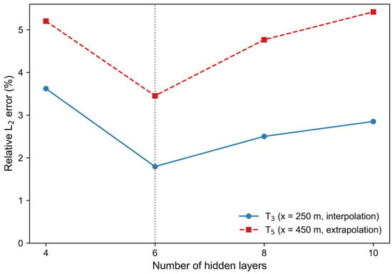
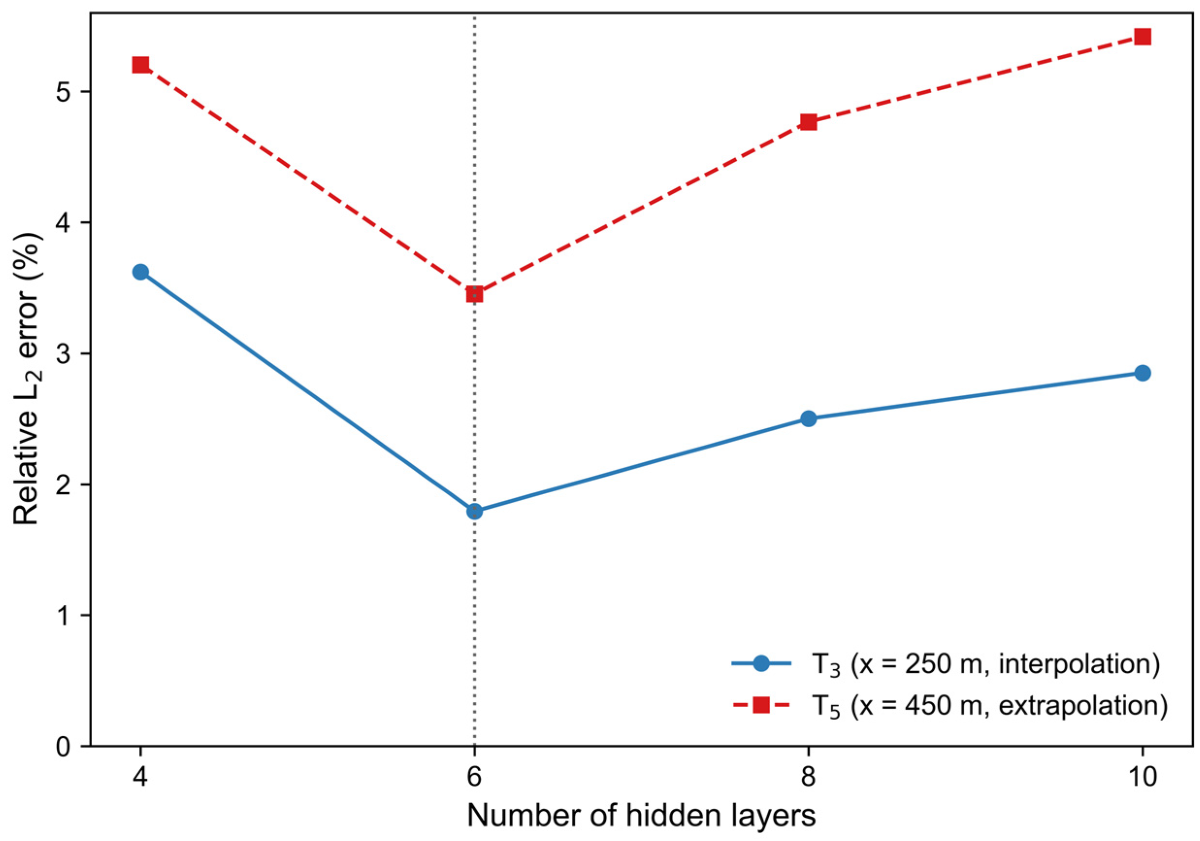
The input–output structure and layer width of twenty neurons were fixed, and the number of hidden layers was set to 4, 6, 8 or 10, with T₁, T₂ and T₄ as observation sections. Accuracy varied non-monotonically with depth (Figure 5). The six-layer network completed training in 75 min, only 5 min longer than the four-layer network, yet gave the lowest relative L₂ error and the most favorable accuracy-cost trade-off. Increasing the depth to eight and ten layers increased the training time to 80 and 88 min, respectively, raising computational cost by 6.7% and 17.3% while reducing accuracy. For the available sparse data, six layers therefore provide sufficient capacity, whereas deeper networks add unnecessary complexity and mild overfitting. The six-layer model also followed surge peaks and troughs at interpolation section T₃ and extrapolation section T₅ more closely than the deeper networks.

Figure 5. Relative L₂ error at the interpolation section T₃ and the extrapolation section T₅ versus the number of hidden layers. Six layers give the lowest error at both sections (dashed line), confirming that reconstruction accuracy is non-monotonic in network depth.

3.2.2. Loss-Term Weights

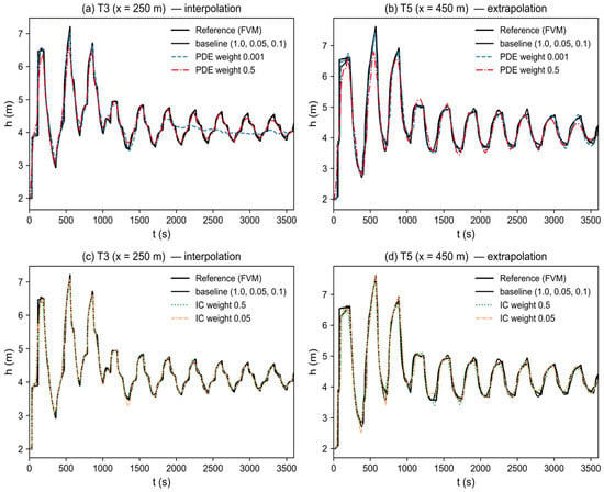
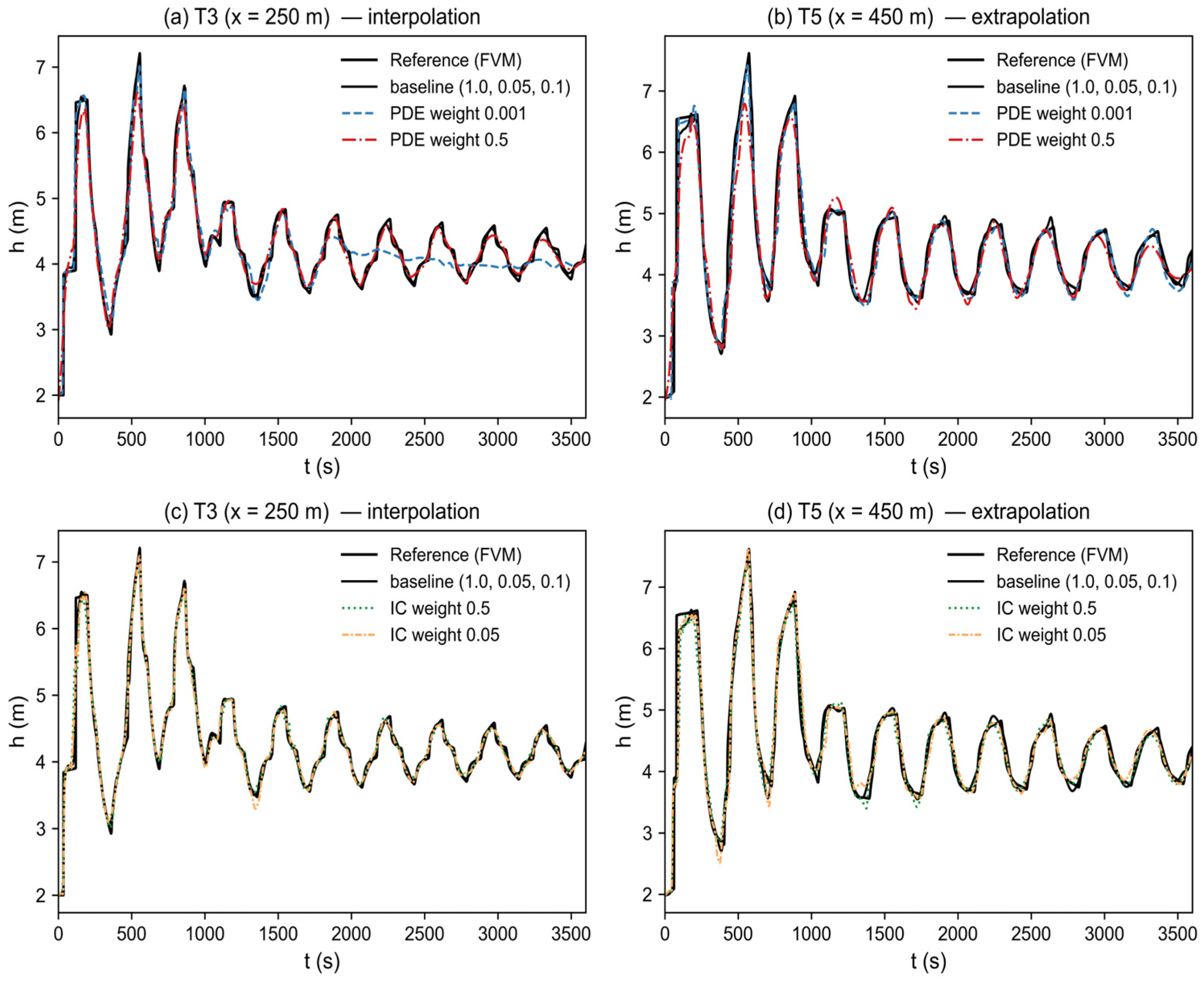
Loss-term weighting strongly affects PINN training because an imbalance can cause the optimizer to favor one term at the expense of the others and impede convergence [38]. With a six-layer network, five weight combinations (Table 2) were compared in a controlled-variable design: groups {1,2,3} varied the PDE weight, and groups {1,4,5} varied the initial-condition weight. Figure 6 compares predicted depth series with the reference. The baseline (group 1) reproduced the surge waveform most closely and produced the lowest relative L₂ error at both interpolation section T₃ and extrapolation section T₅. Reducing the PDE weight by almost two orders of magnitude (group 2) weakened physical regularization substantially. After approximately t = 1300 s, the prediction gradually lost the transient oscillation and drifted towards a flattened, non-physical curve at T₃. Its error was the largest among the PDE-sweep cases, indicating that a weak physical constraint cannot sustain the solution in the sparsely observed interior. Excessively increasing the PDE weight (group 3) had the opposite effect: the loss landscape became too stiff for the optimizer to fit transient observational features, and the extrapolation error increased. Extreme initial-condition weights in groups 4 and 5 did not improve either section. The baseline weights of 1.0, 0.05 and 0.1 therefore provided the best balance between data fidelity and physical constraint.

Table 2. Loss-term weight settings.

Group	${\mathsf{\lambda }}_{\mathbf{data}}$	${\mathsf{\lambda }}_{\mathbf{PDE}}$	${\mathsf{\lambda }}_{\mathbf{IC}}$
1 (baseline)	1.0	0.05	0.1
2	1.0	0.001	0.1
3	1.0	0.5	0.1
4	1.0	0.05	0.5
5	1.0	0.05	0.05

Figure 6. Effect of the loss-term weights on reconstruction, at the interpolation section T₃ (250 m) and the extrapolation section T₅ (450 m). (a,b) PDE-weight sweep (groups 1–3); (c,d) initial-condition-weight sweep (groups 1, 4, 5). The baseline (group 1) tracks the reference most closely at both sections. Reducing the PDE weight (group 2) causes the prediction to drift toward a flattened, non-physical curve at the interpolation section from about t = 1300 s, while over-strengthening it (group 3) degrades the extrapolation prediction; the initial-condition sweep (groups 4, 5) does not improve on the baseline.

3.2.3. Training Budget

Four training budgets, 50,000, 100,000, 500,000 and 1,000,000 iterations, were compared (Table 3). With 50,000 and 100,000 iterations, errors exceeded 4% at interpolation section T₃ and 6% at extrapolation section T₅, and the model failed to learn the waveform after approximately the eighth oscillation cycle. With 1,000,000 iterations, error was low but training time was disproportionately long, and mild overfitting appeared as smoothing that clipped wave peaks. The 500,000-iteration model produced the lowest error at an acceptable training cost and tracked the reference over the full 3600 s.

Table 3. Training time for different iteration budgets (errors from the stored models of this study).

Iterations	50,000	100,000	500,000	1,000,000
Training time	8 min	14 min	80 min	173 min
L2 at T3	0.0488	0.0411	0.0179	0.0235
L2 at T5	0.0733	0.0603	0.0345	0.0413

3.2.4. Standard Configuration

On the basis of these analyses, the configuration in Table 4 was adopted for the training-budget and loss-weight studies. For the validation (Section 3.1) and sensor-placement (Section 3.3) experiments, the eight-hidden-layer architecture was retained so that all reconstruction comparisons share one architecture with the validation model; the network-depth study shows that six layers are optimal in isolation, while eight layers perform comparably at a modestly higher training cost. This is stated explicitly here for reproducibility.

Table 4. Model configuration adopted in this study.

Category	Parameter	Value
Architecture	Hidden layers	6 × 20 neurons
	Activation	Tanh
Optimization	Optimizer	Adam
	Learning rate	1 × 10−3
	Iterations	500,000
	Batch (collocation) size	2048
Loss weights	${\lambda }_{\mathrm{data}}$	1.0
	${\lambda }_{\mathrm{PDE}}$	0.05
	${\lambda }_{\mathrm{IC}}$	0.1

3.3. Sensor-Placement Strategy Under Sparse Observation

3.3.1. Three-Sensor Non-Uniform Strategies

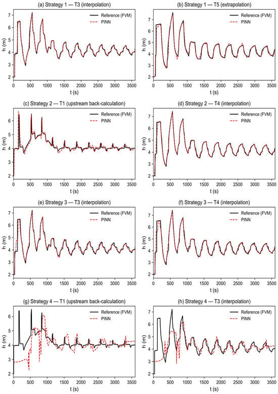
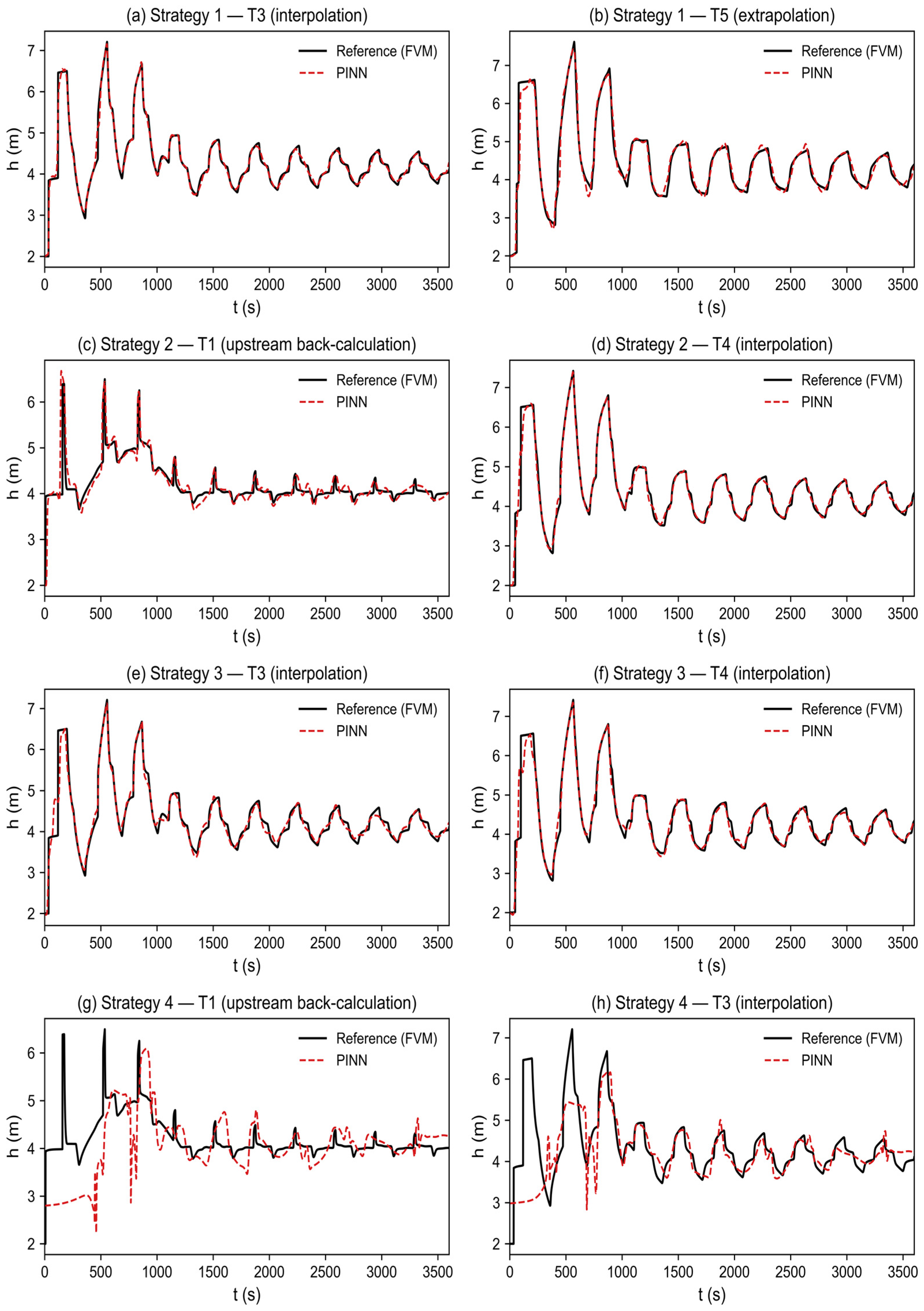
Four deliberately non-uniform three-sensor strategies (Table 5) were designed to examine reconstruction with incomplete boundary information. Their mean L₂ errors at unobserved sections are listed in Table 6. Strategy 3 retained the upstream inlet (T₁) and downstream outlet (T₅), leaving a 300 m interior blind zone, and gave the lowest mean error and best overall reconstruction (Figure 7). In a hyperbolic system governed by the Saint-Venant equations, anchoring both near-boundary sections nearly determines the uniqueness of the full-field solution. The PDE-loss term then propagates boundary information inwards from both ends and stabilizes interpolation in the interior. This result confirms that interpolation is intrinsically easier than extrapolation in this system. Strategies 2 and 4 both omitted the upstream inlet (T₁), allowing us to assess whether the model can infer the upstream boundary from downstream information. Strategy 2, supported by denser observations from the middle to downstream reach, recovered inlet T₁ with moderate error. When interior sensors capture the passing-wave shape, the momentum equation allows the PINN to trace the wave back towards its source. Strategy 4 lacked the inlet and had a sparser interior, with T₂ and T₄ separated by 200 m. It gave the largest error because, with a key boundary missing and the interior sparsely observed, the physical constraint weakens and the model cannot uniquely determine complex upstream inflow from a sparse downstream signal. This contrast shows that inverse reconstruction upstream is much more sensitive to data density than forward propagation. Strategy 1, with the densest upstream coverage, reconstructed mid-channel T₃ well (relative L₂ error approximately 2.5%), but its error at far-downstream T₅ was larger (approximately 4.8%). Without a downstream anchor, physical error accumulated and amplified along the 350–500 m reach, representing the extrapolation risk of an unanchored downstream end. Ranked by mean error across unobserved sections (Table 6), the layouts were strategy 3 (approximately 3.0%) > strategy 1 (approximately 3.7%) > strategy 2 (approximately 5.3%) > strategy 4 (approximately 16.8%).

Table 5. Three-sensor non-uniform placement strategies.

Strategy	Observation Sections	Test Sections
1	{T1, T2, T4}	{T3, T5}
2	{T2, T3, T5}	{T1, T4}
3	{T1, T2, T5}	{T3, T4}
4	{T2, T4, T5}	{T1, T3}

Table 6. Mean L₂ errors of the three-sensor strategies.

Strategy	Test Section	Mean L2 Error
1	T3	2.540902 × 10−2
1	T5	4.763170 × 10−2
2	T1	6.824009 × 10−2
2	T4	3.704768 × 10−2
3	T3	4.498486 × 10−2
3	T4	1.463041 × 10−2
4	T1	1.602583 × 10−1
4	T3	1.758179 × 10−1

Figure 7. Reconstruction under the four three-sensor strategies. Each panel shows the PINN prediction (red dashed) against the finite-volume reference (black solid) at a representative unobserved section. Strategies 1, 2 and 3 reconstruct the transient accurately, whereas strategy 4 (no inlet and sparse interior) fails at the upstream section T₁.

Overall, the boundary-anchored layout of strategy 3 shows that boundary anchoring combined with PDE infilling is an effective approach to sparse reconstruction. Strategy 2 shows that, even without the upstream inlet, the PINN can infer the inlet with moderate error and retain useful inverse-reconstruction accuracy provided that interior observations are sufficiently continuous. Strategy 1 shows that, even without a downstream anchor, dense upstream coverage supports interior interpolation. Together, these results indicate practical fault tolerance. Strategy 4 provides a cautionary example: monitoring-network design should avoid both missing a key boundary and using overly sparse interior coverage, because this combination weakens the physical constraint and allows errors to diverge.

3.3.2. Two-Sensor Strategies, Spatial Topology, and Noise Robustness

To examine the reconstruction limit under extreme sparsity, all ten two-sensor combinations of the five candidate sections were enumerated and classified by spatial topology, from complete boundary control to purely interior observation (Table 7). To emulate unavoidable measurement error, zero-mean Gaussian white noise was added to clean observation series during training,

$$h_{\mathrm{noisy}}=h_{\mathrm{clean}}+\eta \hspace{0.17em}\sigma \hspace{0.17em}\mathcal{N}\left(\mathrm{0,1}\right)$$

(15)

where $\mathcal{N}(0,1)$ is the standard normal distribution, $\sigma$ is the standard deviation of the original depth series at the sensor, and $\eta$ is the noise level, set to 0.05, 0.10, and 0.20, that is, 5%, 10%, and 20%.

Table 7. Two-sensor placement strategies and their topological classification.

Strategy	Sensors (T)	Positions (m)	Boundary-Condition Feature
1	{1,2}	{50,150}	inlet only, upstream-dense
2	{4,5}	{350,450}	outlet only, downstream-dense
3	{1,5}	{50,450}	full inlet + outlet
4	{2,5}	{150,450}	outlet only, long-range back-calculation
5	{2,3}	{150,250}	no boundary, upstream-local
6	{2,4}	{150,350}	no boundary, large span
7	{1,3}	{50,250}	inlet only, mid-range extrapolation
8	{1,4}	{50,350}	inlet only, long-range extrapolation
9	{3,5}	{250,450}	outlet only, short-range back-calculation
10	{3,4}	{250,350}	no boundary, downstream-local

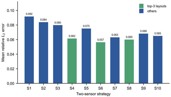
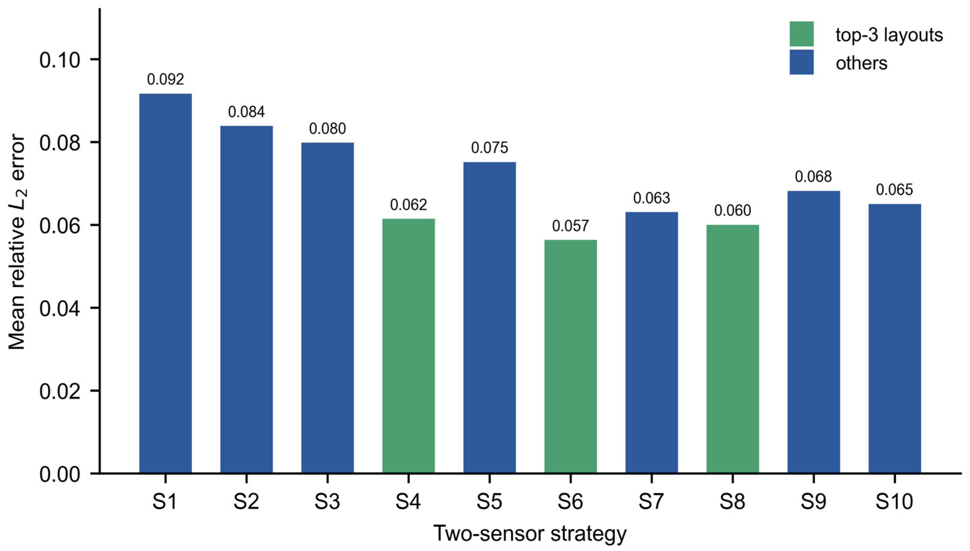
Under 5% noise, the three best layouts were strategies 4, 6 and 8 (Figure 8). Strategy 6, with sensors T₂ and T₄ at 30% and 70% of the conduit length, provided the most uniform spatial coverage. Strategies 4 and 8 placed a sensor near the downstream and upstream boundaries, respectively, widening the sensing envelope while retaining reasonably uniform spacing. These layouts formed the experimental group. Strategy 3, which used the two sensors nearest the boundaries, served as the control for the noise-intensity sensitivity analysis.

Figure 8. Mean relative L₂ error over the unobserved sections for all ten two-sensor strategies under 5% training noise. The three lowest-error layouts (strategies 4, 6 and 8; green) are selected for the noise-intensity analysis.

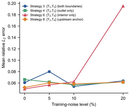
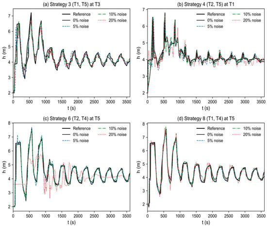
Figure 9 summarizes the mean error of the four representative layouts as noise level increases, and Figure 10 shows the corresponding waveforms. Strategy 3 anchors the inlet at 50 m and outlet at 450 m and was highly robust in the single runs. Even with 20% noise, predicted depth series remained accurate, with only small peak-amplitude deviations and no severe non-physical oscillations. Anchoring both near-boundary sections constrains characteristic evolution and allows information to propagate stably from both ends towards the interior. Notably, in the single runs the model trained with 10% noise generalized slightly better than that trained with 5% noise; the statistical meaning of this observation is examined in Section 3.3.3, where repeated runs show that it reflects the noise realization rather than a systematic benefit.

Figure 9. Mean relative L₂ error at the unobserved sections versus the training-noise level, for four representative two-sensor strategies. The boundary-anchored strategies 3 and 8 stay accurate up to 20% noise, whereas the interior-only strategy 6 degrades sharply at 20%.

Figure 10. Waveform robustness to training noise for four representative two-sensor layouts, each shown at a diagnostic unobserved section. (a) Full-boundary strategy 3 (T₁, T₅) at T₃ and (d) upstream-anchored strategy 8 (T₁, T₄) at T₅ stay close to the reference at 0%, 10% and 20% noise. (b) Outlet-only strategy 4 (T₂, T₅) leaves a persistent upstream error at T₁ and develops non-physical oscillations at 20% noise. (c) Interior-only strategy 6 (T₂, T₄) is accurate at 0% and 10% but collapses into large non-physical oscillations at T₅ under 20% noise. Reference: black solid; predictions colored by noise level. Anchoring a boundary, and especially the upstream boundary, confines the noise-driven error, whereas the interior-only layout must extrapolate to both ends and amplifies it.

By contrast, strategy 6, which used interior-only sensors T₂ and T₄, achieved good interpolation accuracy under low noise because of uniform spacing. Under 20% noise, however, its predictions deteriorated sharply at both ends near T₁ and T₅ and developed large non-physical oscillations; downstream error increased several-fold relative to the low-noise case. Without direct boundary constraints, the model must extrapolate in both directions. In a hyperbolic system, this bidirectional extrapolation is ill-posed and amplifies observation noise. Strategy 4, with sensors T₂ and T₅, anchors only the downstream boundary. It retained low outlet error but had a persistently larger error in the upstream blind zone at T₁, where clear non-physical oscillations appeared with 20% noise. Downstream control cannot fully constrain ill-posed inverse propagation upstream, although this partial anchoring avoided the catastrophic breakdown seen with the interior-only layout. Strategy 8, with sensors T₁ and T₄, gave the best overall robustness in the single runs. By anchoring the upstream boundary at T₁, the model need only propagate downstream along the Saint-Venant characteristics. Thus, even with 20% noise, predictions at interpolation sections T₂ and T₃ and downstream extrapolation section T₅ closely followed the reference. With limited monitoring resources, a non-uniform layout including the upstream boundary node, such as strategy 8, is therefore more noise-robust and more suitable for engineering applications than a uniform interior-only layout, such as strategy 6—with the caveat on 10%-noise failure modes quantified in Section 3.3.3.

3.3.3. Statistical Stability of the Reconstruction

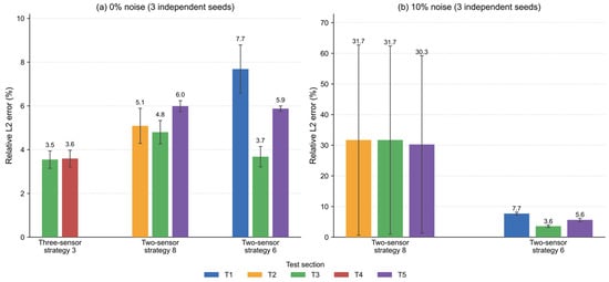
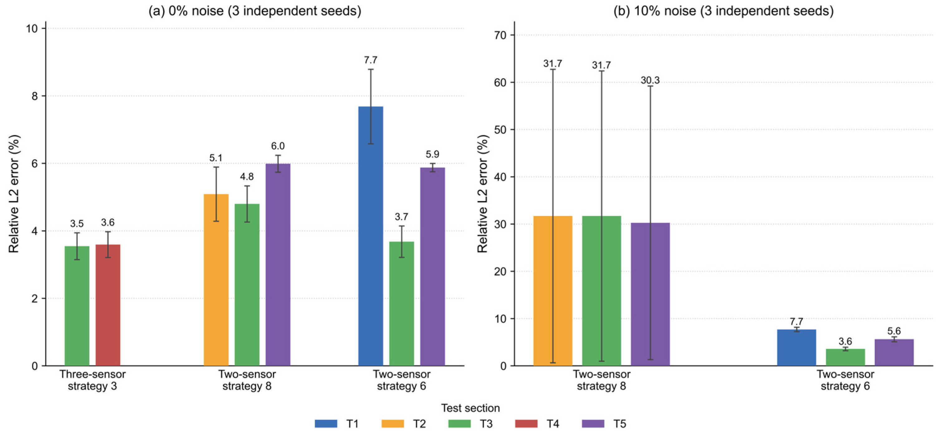
Because PINN training and noise injection are stochastic, representative configurations were retrained with three independent random seeds (all random streams—network initialization, collocation resampling, noise realizations—were reseeded). Table 8 reports the mean and standard deviation of the relative L₂ errors at the unobserved sections (Figure 11).

Table 8. Mean ± standard deviation of relative L₂ errors over three independent seeds (0% noise; 10% noise where indicated).

Configuration	Test Sections	Mean ± Std (%)
Three-sensor strategy 3 (0%)	T3/T4	3.55 ± 0.40/3.59 ± 0.38
Two-sensor strategy 8 (0%)	T2/T3/T5	5.09 ± 0.80/4.80 ± 0.54/5.99 ± 0.25
Two-sensor strategy 8 (10%)	T2/T3/T5	31.7 ± 31.1/31.7 ± 30.7/30.3 ± 28.9 (2 of 3 runs < 16%)
Two-sensor strategy 6 (0%)	T1/T3/T5	7.68 ± 1.10/3.68 ± 0.46/5.88 ± 0.12
Two-sensor strategy 6 (10%)	T1/T3/T5	7.71 ± 0.56/3.58 ± 0.46/5.63 ± 0.64

Figure 11. Mean and standard deviation (error bars) of the relative L₂ errors over three random seeds for the repeated configurations. At 0% noise, all configurations are stable; at 10% noise, strategy 8 shows one spurious run out of three (large error bars), while strategy 6 remains stable.

At 0% noise, the reconstruction is statistically stable. Three-sensor strategy 3 yields 3.55% ± 0.40% at T₃ and 3.59% ± 0.38% at T₄ (the single-run values reported in Table 6, 4.50% and 1.46%, lie within a few standard deviations of these means), and the two-sensor strategies 8 and 6 give means of 4.8–6.0% and 3.7–7.7%, with standard deviations below 1.1%. The rankings among layouts reported in Section 3.3.1 and Section 3.3.2 are therefore reproduced across seeds: boundary-anchored layouts outperform interior-only layouts on average.

At 10% noise, however, the repeated runs reveal a failure mode that the single-run experiments could not show. For strategy 8, two of the three runs retained low errors (5.6–15.7% at the test sections), but one run converged to a spurious solution with errors of 70–75%, even though its composite loss decreased normally to 9 × 10⁻³. In that run, the network satisfied the PDE residual and the noisy data while locking onto a wrong wave pattern—a non-uniqueness mode of the sparse noisy inverse problem, in which the initial condition alone (enforced only at t = 0) is insufficient to select the correct branch. This confirms that the occasional improvement at 10% noise reported for single runs reflects the noise realization and random initialization rather than a systematic benefit. The practical implication is that, at moderate noise levels, the boundary-anchored two-sensor layouts are robust in most runs but require safeguards—multiple restarts with the lowest-data-loss solution selected, or a third sensor—before deployment. By contrast, the interior-only strategy 6 was stable at 10% noise in all three runs (7.71% ± 0.56% at T₁, 3.58% ± 0.46% at T₃, 5.63% ± 0.64% at T₅), essentially indistinguishable from its 0%-noise results. This contrast is mechanistically informative: strategy 8 concentrates its two observations near the ends of the domain and leaves a 300 m interior blind zone, so that, at 10% noise, a wrong interior wave pattern becomes a viable branch; strategy 6 places its sensors uniformly in the interior, which constrains the wave shape more evenly and, at this noise level, avoids the spurious branch at the cost of weaker boundary information. Boundary anchoring therefore provides the highest accuracy and noise robustness overall, but under moderate noise a layout with a large observation-free interior span carries a small but non-negligible risk of converging to a spurious branch, whereas a uniformly spaced interior layout is more predictable, if somewhat less accurate.

3.3.4. Sensors at the True Boundaries

Because T₁ and T₅ are boundary-adjacent rather than boundary sensors, four additional layouts with sensors at the true domain boundaries (x = 0 and x = 500 m) were trained on the full-field reference data, using the same architecture and training settings as the two-sensor study. Table 9 reports the relative L₂ errors, and Figure 12 shows representative waveforms.

Table 9. Relative L₂ errors (%) at unobserved sections for layouts with true-boundary sensors.

Layout	Test Sections	L2 Errors (%)
{x = 0, 500 m} (two sensors)	50/150/250/350/450 m	5.33/8.60/8.73/6.56/3.37
{x = 0, 350 m} (two sensors)	150/250/450/500 m	8.13/6.00/6.96/9.35
{x = 150, 500 m} (two sensors)	0/50/250/350 m	9.18/6.58/4.64/4.78
{x = 0, 250, 500 m} (three sensors)	50/150/350/450 m	4.74/4.60/3.64/3.05
{x = 0, 350 m} at 10% noise	150/250/450/500 m	6.46/5.27/6.77/8.69

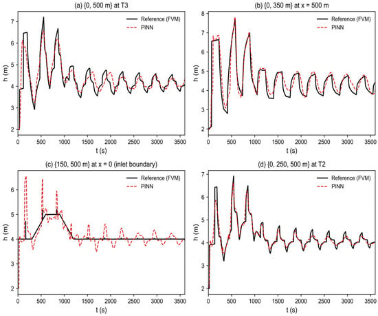
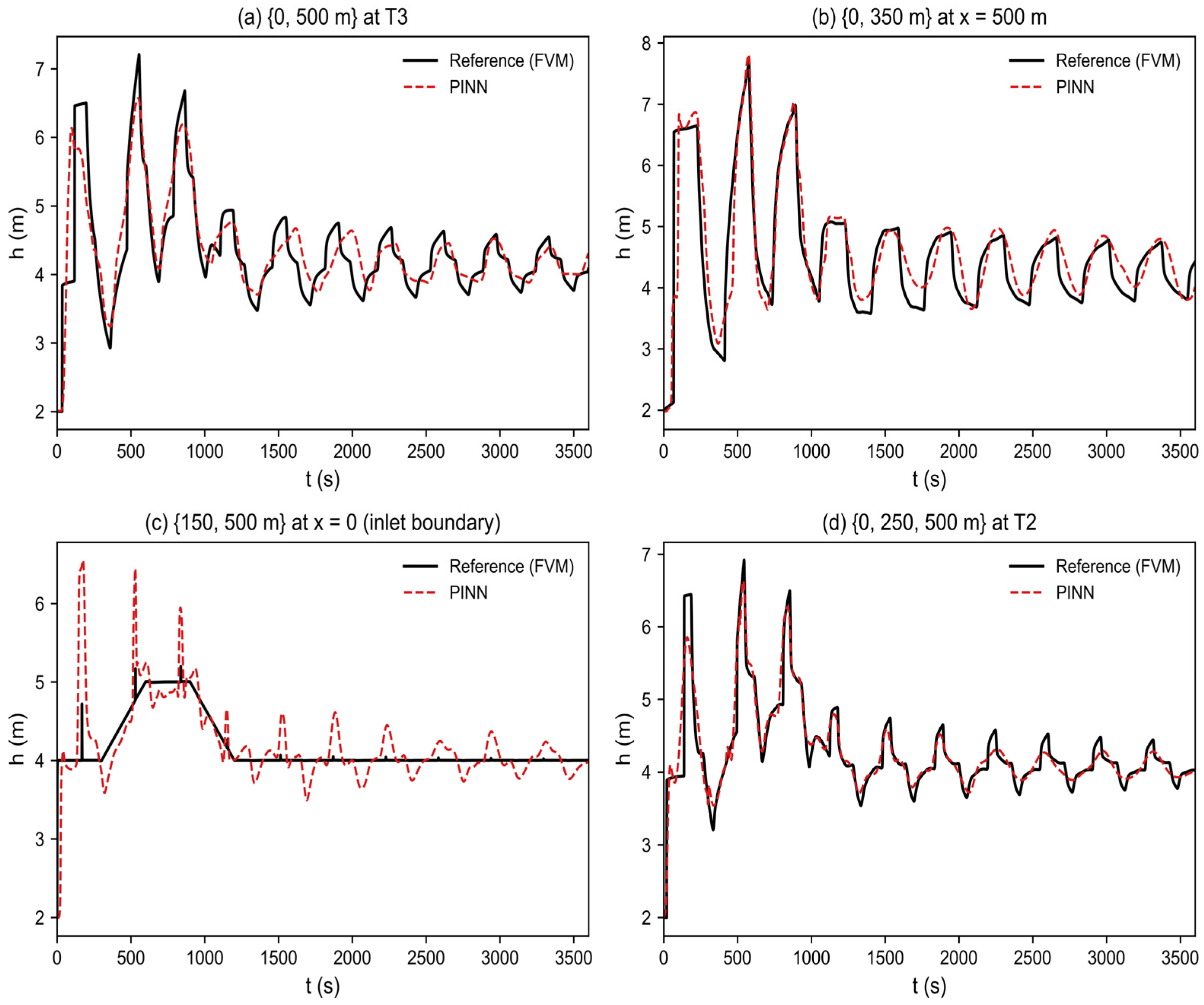
Figure 12. Reconstruction with sensors at the true boundaries (x = 0 and 500 m). (a) Two-sensor {0, 500 m} at T₃; (b) up-stream-anchored {0, 350 m} at x = 500 m; (c) downstream-anchored {150, 500 m} at x = 0 (inlet boundary); and (d) three-sensor {0, 250, 500 m} at T₂. Reference: black solid; PINN: red dashed.

The two-sensor layout {x = 0, x = 500} reconstructs the whole domain with errors of 3.4–8.7% across the five diagnostic sections—confirmation that two true boundary sensors, combined with the PDE constraint, are sufficient to reconstruct the interior field. The single-upstream-boundary layout {x = 0, x = 350} reconstructs the downstream end (x = 500 m) with 9.4% error, while the single-downstream-boundary layout {x = 150, x = 500} reconstructs the inlet boundary (x = 0) with 9.2% error and the near-inlet section T₁ (x = 50 m) with 6.6%: consistent with the mechanism of Section 3.4, information propagates more reliably downstream than upstream, so securing the upstream boundary is the priority. At the inlet, the reference depth is the externally controlled water-level boundary—a step-and-ramp hydrograph—rather than a wave-dynamical response, so the inlet is the hardest section for any interior-data-driven inference; the 9.2% error quantifies this difficulty, and Figure 12c displays the reconstruction at the inlet boundary itself. The three-sensor layout {x = 0, x = 250, x = 500} is the most accurate of the group (3.1–4.7%). At 10% noise, the up-stream-anchored {x = 0, x = 350} remains stable (5.3–8.7%). These results confirm that the placement principle established with boundary-adjacent sensors—anchor the upstream boundary first—carries over to true boundary sensors. The results also strengthen the claim that boundary anchoring, rather than the specific sensor positions of T₁–T₅, is the operative mechanism.

3.4. Discussion: Mechanism, Generality, and Limitations

The results in Section 3.1, Section 3.2 and Section 3.3 point to a common mechanism. The Saint-Venant system is hyperbolic, and information propagates along characteristics originating at the domain boundaries. A boundary sensor provides a well-determined origin for these characteristics, and the PDE-residual loss subsequently carries this information into the interior. This mechanism explains why boundary-anchored layouts—three-sensor strategy 3, two-sensor strategy 8, and, in the new boundary-sensor experiments (Section 3.3.4), the layouts anchored at the true boundaries—were both most accurate and most robust to noise. By contrast, interior-only layouts such as strategy 6 force the network to perform ill-posed bidirectional extrapolation, which amplifies noise. The resulting practical principle is to secure the upstream boundary first and then broaden the sensing envelope. Because this principle follows from the governing-equation structure rather than from the specific case, it may transfer to other advection-dominated free-surface conveyance systems. It may not apply unchanged to strongly diffusive regimes or multidimensional flows, which are outside the scope of this study.

The apparent noise benefit in the single-run experiments of Section 3.3.2 must be interpreted with care. The repeated-seed experiments of Section 3.3.3 show that, at 0% noise, all runs of the boundary-anchored strategies stay accurate (standard deviations ≤ 1.1%), whereas, at 10% noise, one of three runs of strategy 8 converged to a spurious solution with errors above 70% although its composite loss decreased normally. The occasional slight improvement at 10% noise observed in single runs therefore reflects the noise realization and random initialization rather than a systematic benefit; it should not be read as a recommendation to add noise. The more robust reading is that, in most runs, moderate observation noise does not degrade the boundary-anchored reconstruction appreciably, because the physics residual regularizes the noisy data term; but sparse noisy configurations admit spurious branches, and safeguards such as multiple restarts or an additional sensor are advisable. This failure mode is a property of the two-sensor, 10%-noise configuration tested here and was observed for the layouts and scenario of this study.

The friction-closure question discussed in Section 3.5 deserves emphasis: the momentum balance of the present scenario is dominated by the pressure, convective and inertia terms, so the reconstruction is insensitive to whether a steady Darcy or a Brunone-type closure is used, as confirmed by the friction ablation. This is a property of the slowly varying flood-rise transient studied here, not a general statement about unsteady friction in free-surface flow; fast surge fronts or mixed-flow transitions may require an acceleration-based closure, whose open-channel calibration remains an open research question.

Several limitations qualify these conclusions and indicate directions for future work. The reference data are high-resolution numerical solutions rather than field measurements; although the reference solver is verified through grid convergence, discrete conservation and a cross-method MOC check, the absolute errors may be optimistic and require confirmation with experimental or operational data. The comparison in Section 3.1 is a controlled physics ablation against an identical network without the physics loss, not a benchmark against classical data-assimilation methods (adjoint/variational, Kalman-type), Gaussian-process or interpolation methods, recurrent networks or neural operators; such benchmarks are planned as future work. The study also considers a single circular conduit under one flood-rise scenario (plus the four cross-scenario tests of Section 3.5), and the model requires retraining or fine-tuning when boundary or initial conditions change substantially. Finally, the method is an offline reconstruction tool that uses complete observation histories; causal (streaming-data) assimilation and its combination with classical data-assimilation uncertainty estimates remain open. Future work should validate the approach with field data, examine additional geometries (including mixed-flow and wet–dry regimes, where well-balanced positivity-preserving schemes [29] become necessary), compare it with stronger baselines, extend it to branched and looped networks, and assess online assimilation of streaming data.

3.5. Reliability of the Reference Solution and Cross-Scenario Tests

The credibility of the reconstruction results rests on the reliability of the reference FVM solution and on the generality of the conclusions beyond the single training scenario. Both are examined here.

3.5.1. Reliability of the Reference Solution

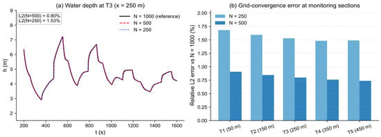
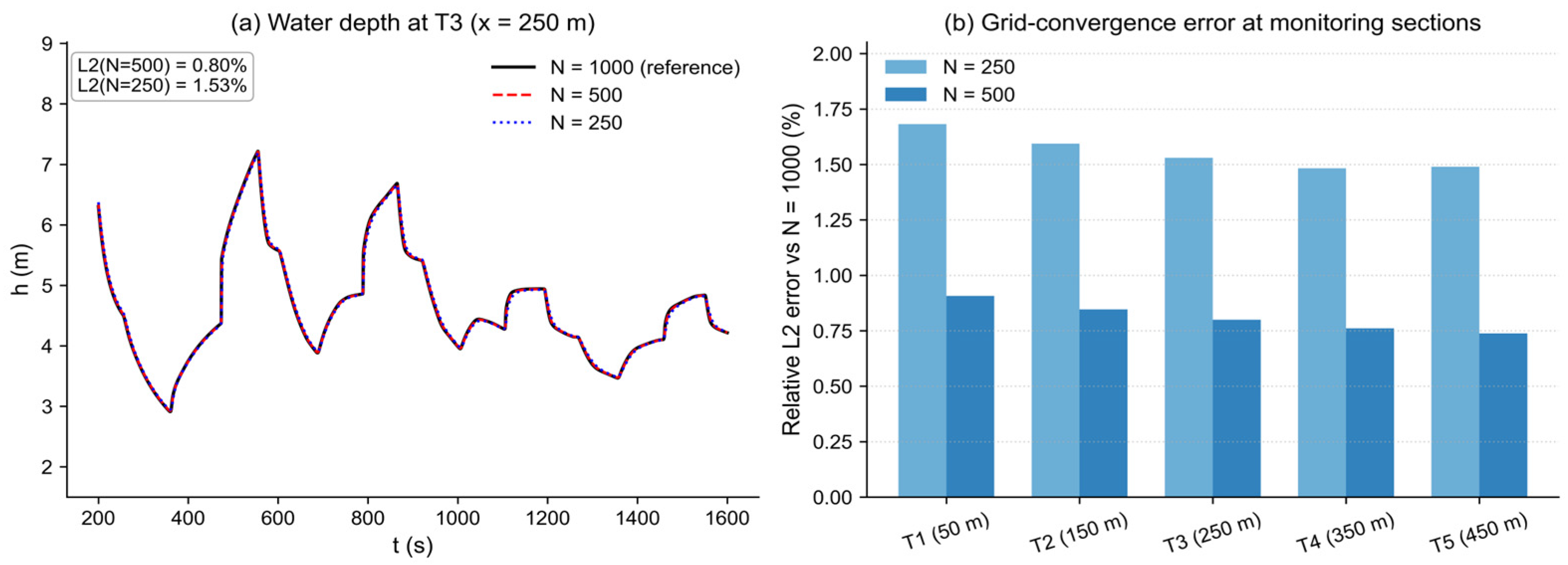
To establish the reliability of the reference solution, the forward solver was re-run with N = 250 and N = 1000 cells and compared with the N = 500 solution used elsewhere in this study. Figure 13a shows the water-depth series at T₃ during the flood-rise window for the three resolutions; the solutions are visually indistinguishable. Quantitatively, the relative L₂ difference against the N = 1000 solution decreases from 1.53% (N = 250) to 0.80% (N = 500) at T₃, with similar values at all five monitoring sections (Figure 13b, Table 10). The monotone convergence indicates that N = 500 adequately resolves the transient.

Figure 13. FVM grid convergence. (a) Water depth at T₃ for N = 250, 500 and 1000 cells during the flood-rise window; (b) relative L₂ error of the N = 250 and N = 500 solutions against the N = 1000 solution at the five monitoring sections.

Table 10. Diagnostic checks of the reference solution and of the reconstructed field.

Quantity	Value
Froude-number range (mean)	0–0.81 (0.12), subcritical throughout
Water-depth range	2.0–7.7 m
Grid convergence, N = 500 vs. N = 1000 (T3)	0.80% relative L2
Discrete mass-balance closure (RMS, relative to inlet flux)	1.1%
Time-discretization difference (adaptive vs. uniform sampling)	<0.3%
MOC vs. FVM, global relative L2	≈14%
PINN peak-amplitude error at T5	−3.1%
PINN peak-time lag at T5	−7.6 s
PINN cross-correlation lag at T5	0.6 s
PINN RMS mass residual (normalized by ∂A/∂t scale)	0.67

As a second check, the discrete mass-balance closure dV/dt − Q_in (where V is the stored water volume and Q_in the inlet flux; the outlet is closed) was evaluated from the full-resolution solution saved at every adaptive step: its RMS value is 1.1% of the RMS inlet flux (Table 10), as expected for an explicit HLL update with source splitting, and the largest closure error occurs at the initial level step at the inlet. Comparing the adaptive-step series with the uniformly sampled series used for the full-field data shows differences below 0.3% at all sections, i.e., the output sampling does not degrade the reference series (Table 10).

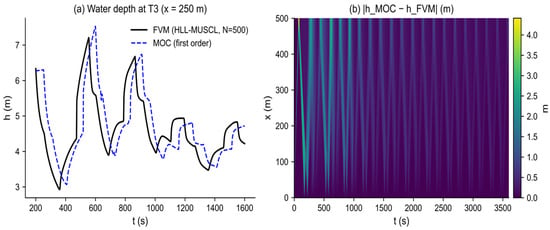
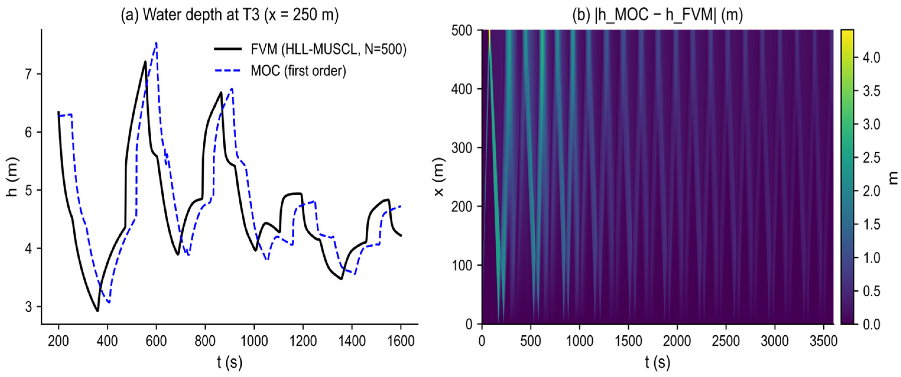
As an independent cross-method check, a first-order method-of-characteristics (MOC) implementation of the same initial-boundary-value problem, with the same Darcy–Weisbach closure, yields a global relative L₂ difference of ≈14% from the FVM solution, with the differences concentrated at the steep surge fronts where the first-order MOC dissipates the peaks (Figure 14). This quantifies the method-related uncertainty of the reference solution: the second-order HLL–MUSCL solution is the more accurate of the two (see Figure 13 and the conservation check), but the comparison shows that the wave structure and timing are robust across independent numerical methods. The absolute accuracy of the reference solution cannot be certified further without experimental or operational data; this is stated as a limitation.

Figure 14. Cross-method check of the reference solution. (a) Water depth at T₃ from the FVM solution and from an independent first-order MOC implementation of the same problem; (b) absolute difference |h_MOC − h_FVM| over the full space–time domain, concentrated at the steep surge fronts.

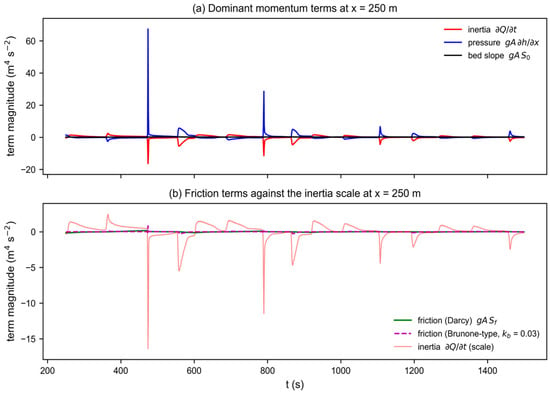
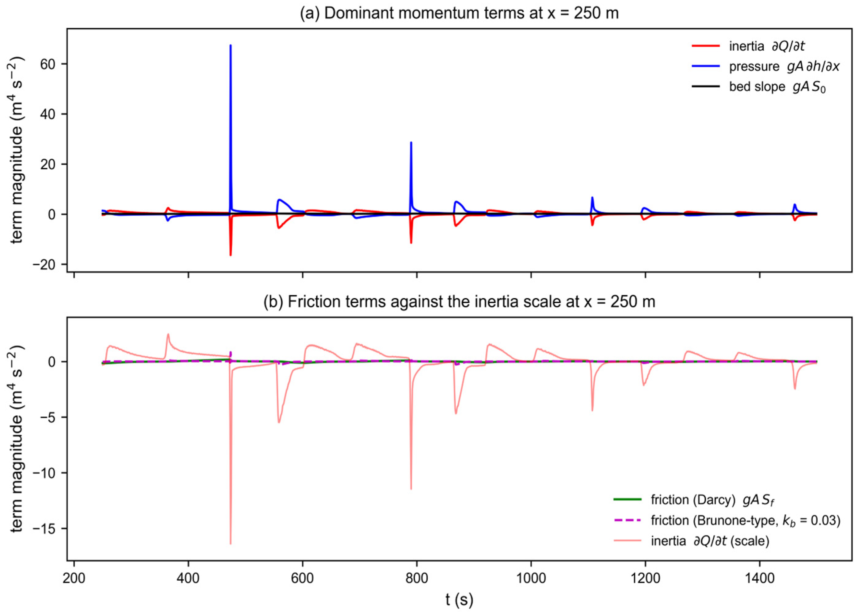
Returning to the friction-closure question of Section 2.2, the momentum Equation (2) was evaluated term by term from the reference solution over the full space–time domain (Table 11). The pressure term gA∂h/∂x, the convective term and the local-inertia term ∂Q/∂t dominate, with RMS values 13–26 times the bed-slope term gA S₀; the Darcy friction term is 43% of the bed-slope term and ≈3.3% of the inertia term, and a Brunone-type term with the free-surface adaptation of Equation (7) and k_b = 0.03–0.05 is 0.7–1.2 times the bed-slope term and ≈5.4–9.1% of the inertia term (Figure 15). Friction is thus a second-order contributor to the momentum balance of this slowly varying transient (Figure 15, Table 11). As a direct check, a PINN was retrained with the Brunone-type term included in the momentum residual (friction ablation): the resulting errors at T₃ and T₅ are 3.88% and 6.06%, slightly worse than the Darcy baseline (2.50% and 4.77%). The unsteady term therefore does not improve the reconstruction, confirming that the steady closure is adequate for this scenario. Because no calibrated k_b exists for open-channel flow, the steady Darcy closure was retained; unsteady friction may become necessary for fast surge fronts or mixed-flow transitions, as is discussed among the future directions.

Table 11. Term-wise RMS of the momentum Equation (2) over the full space–time domain, computed from the reference solution (units m³ s⁻²).

Term	RMS	Relative to Bed-Slope Term
∂Q/∂t (inertia)	1.82	13.1
∂(Q2/A)/∂x (convection)	2.21	15.9
gA∂h/∂x (pressure)	3.61	25.9
gA S0 (bed slope)	0.139	1.0
gA Sf, Darcy friction	0.060	0.43
Brunone-type, kb = 0.03	0.099	0.71
Brunone-type, kb = 0.05	0.165	1.19

Figure 15. Term-wise momentum balance at x = 250 m during the flood-rise window, computed from the reference solution. (a) Dominant terms: inertia ∂Q/∂t, pressure gA∂h/∂x and bed slope gA S₀; (b) friction terms (Darcy and Brunone-type with k_b = 0.03) against the inertia scale. Friction is a second-order contributor to the momentum balance of this slowly varying transient.

3.5.2. Ablation and Cross-Scenario Generality

Turning to the components of the PINN itself, removing the initial-condition term (λ_IC = 0) changes the validation errors from 2.50%/4.77% to 1.68%/5.76% at T₃/T₅: the reconstruction is essentially unaffected, because the observation series and the PDE constraint already determine the field, and the IC term only assists the earliest transient near the inlet. This ablation confirms that the data and PDE terms are the operative constraints in the present setup.

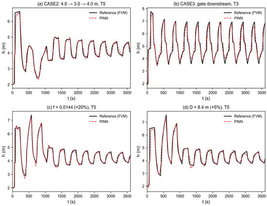
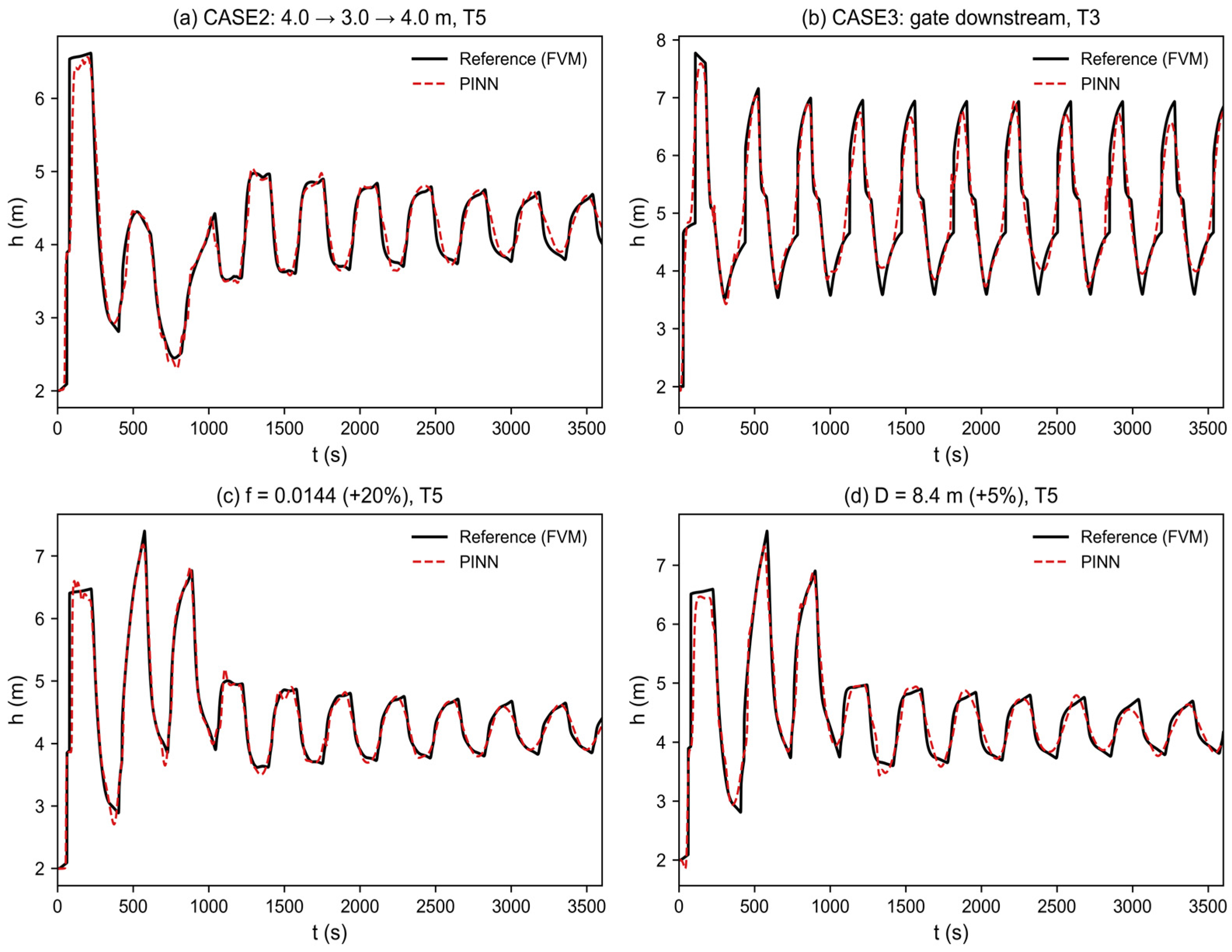
Finally, the standard PINN configuration was retrained, without any change, on four additional scenarios generated by the same solver family: CASE2, a falling-water perturbation (4.0 → 3.0 → 4.0 m) with the same wall outlet; CASE3, a constant 5.0 m upstream level with a downstream gate; a +20% perturbation of the friction factor (f = 0.0144); and a +5% perturbation of the diameter (D = 8.4 m). The relative L₂ errors at T₃/T₅ are 3.67%/5.92% (CASE2), 5.93%/8.95% (CASE3), 2.31%/5.05% (f + 20%) and 3.79%/5.79% (D + 5%), all of the same order as the baseline scenario (2.50%/4.77%). Figure 16 shows representative reconstructions. The reconstruction accuracy transfers to these scenarios, indicating that the method is not tuned to the specific flood-rise case and that the conclusions are not an artifact of the reference model’s parameter values.

Figure 16. Generalization to independent scenarios with the same PINN configuration. (a) CASE2 (falling-water perturbation) at T₅; (b) CASE3 (gated outlet) at T₃; (c) f = 0.0144 (+20%) at T₅; (d) D = 8.4 m (+5%) at T₅. Reference: black solid; PINN: red dashed.

4. Conclusions

This study developed a physics-informed neural network coupled with the one-dimensional Saint-Venant equations, closed by a Darcy–Weisbach steady friction term in hydraulic-radius form, to reconstruct transient water-depth fields in long-distance free-surface conveyance tunnels. By embedding the governing equations as a soft constraint in the loss function, the model reconstructs the complete field from sparse depth observations under physical constraints. Its behavior was characterized across network topology, noise conditions and sensor layouts, and the credibility of the reference solution and the generality of the conclusions were verified through dedicated checks. The main findings are as follows.

• The PINN mitigates the overfitting of purely data-driven methods under sparse sampling. With only a few monitoring sections, it accurately reconstructs water-depth evolution in unobserved regions and reduces relative L₂ error to approximately one-quarter of that of an equivalent ANN at both interpolation (2.50% vs. 10.05%) and extrapolation (4.77% vs. 13.69%) sections. A controlled ablation identifies the embedded physics as the source of this advantage, and the advantage is robust: repeated runs under three random seeds reproduce the ranking of the layouts, and peak-timing and residual checks confirm that wave amplitude and phase are captured.
• Sensor placement is decisive for reconstruction robustness. A layout including the upstream boundary—whether boundary-adjacent (strategy 8) or at the true boundary (x = 0)—is markedly more robust to noise than an interior-only layout (strategy 6), because boundary anchoring suppresses noise amplification during inverse extrapolation. Layouts anchored at both true boundaries (x = 0 and 500 m) reconstruct the whole domain accurately from two sensors alone.
• The model shows substantial tolerance to noise. Under the physical regularization imposed by the governing equations, moderate observation noise (up to 10–20% for boundary-anchored layouts) does not cause prediction divergence in most runs. Repeated-seed experiments show stable low errors at 0% noise (standard deviations ≤ 1.1%) but reveal that a minority of trainings at 10% noise converge to spurious solutions; the occasional slight improvement at 10% noise in single runs is a realization effect, not a systematic benefit. Safeguards such as multiple restarts or an additional sensor are recommended at higher noise levels.
• The conclusions rest on a verified reference solution: grid refinement (N = 250–1000) converges monotonically (0.8% difference at N = 500), the discrete mass balance closes to 1.1%, and an independent MOC solution confirms the wave structure. The friction closure is a second-order term in the momentum balance of this slowly varying transient, and a friction-closure ablation confirms that the reconstruction is insensitive to whether a steady Darcy or a Brunone-type term is used; the free-surface adaptation of acceleration-based friction is provided for future use in fast transients. Cross-scenario tests (falling-water perturbation, gated outlet, perturbed friction and geometry) show that the method transfers without retuning.

These results provide a basis for intelligent monitoring and soft-sensor development in free-surface conveyance tunnels, as an offline reconstruction tool. Limitations remain, however. This study relies on numerical reference data and considers a single conduit focusing on water depth h; validation against field or experimental data is required before operational deployment. Extension to branched and looped conveyance networks, mixed-flow and wet–dry regimes, benchmark comparisons with classical data-assimilation methods and neural operators, and causal online assimilation of streaming data remain subjects for future work.

References

- Courtier, P.; Talagrand, O. Variational assimilation of meteorological observations with the direct and adjoint shallow-water equations. Tellus A 1990, 42, 531–549. [Google Scholar] [CrossRef] [Scilit]
- Wylie, E.B.; Streeter, V.L. Fluid Transients in Systems; Prentice Hall: Englewood Cliffs, NJ, USA, 1993. [Google Scholar]
- Hodges, B.R. Conservative finite-volume forms of the Saint-Venant equations for hydrology and urban drainage. Hydrol. Earth Syst. Sci. 2019, 23, 1281–1304. [Google Scholar] [CrossRef] [Scilit]
- Li, X.; Xu, W.; Ren, M.; Jiang, Y.; Fu, G. Hybrid CNN-LSTM models for river flow prediction. Water Supply 2022, 22, 4902–4919. [Google Scholar] [CrossRef] [Scilit]
- Luo, J.; Zhu, D.; Li, D. Classification-enhanced LSTM model for predicting river water levels. J. Hydrol. 2025, 650, 132535. [Google Scholar] [CrossRef] [Scilit]
- Baek, S.-S.; Pyo, J.; Chun, J.A. Prediction of water level and water quality using a CNN-LSTM combined deep learning approach. Water 2020, 12, 3399. [Google Scholar] [CrossRef] [Scilit]
- Raissi, M.; Perdikaris, P.; Karniadakis, G.E. Physics-informed neural networks: A deep learning framework for solving forward and inverse problems involving nonlinear partial differential equations. J. Comput. Phys. 2019, 378, 686–707. [Google Scholar] [CrossRef] [Scilit]
- Karniadakis, G.E.; Kevrekidis, I.G.; Lu, L.; Perdikaris, P.; Wang, S.; Yang, L. Physics-informed machine learning. Nat. Rev. Phys. 2021, 3, 422–440. [Google Scholar] [CrossRef] [Scilit]
- Cuomo, S.; Di Cola, V.S.; Giampaolo, F.; Rozza, G.; Raissi, M.; Piccialli, F. Scientific machine learning through physics-informed neural networks: Where we are and what’s next. J. Sci. Comput. 2022, 92, 88. [Google Scholar] [CrossRef] [Scilit]
- Jagtap, A.D.; Karniadakis, G.E. Extended physics-informed neural networks (XPINNs): A generalized space-time domain decomposition based deep learning framework for nonlinear partial differential equations. Commun. Comput. Phys. 2020, 28, 2002–2041. [Google Scholar] [CrossRef] [Scilit]
- Waqar, M.; Louati, M.; Ghidaoui, M.S. Physics-informed neural network model for transient wave propagation in pressurized pipeline. In Proceedings of the 39th IAHR World Congress, Granada, Spain, 19–24 June 2022; International Association for Hydro-Environment Engineering and Research (IAHR): Madrid, Spain, 2022; pp. 1748–1757. [Google Scholar] [CrossRef] [Scilit]
- Ye, J.; Do, N.C.; Zeng, W.; Lambert, M. Physics-informed neural networks for hydraulic transient analysis in pipeline systems. Water Res. 2022, 221, 118828. [Google Scholar] [CrossRef] [Scilit] [PubMed]
- Ye, J.; Zeng, W.; Do, N.C.; Lambert, M. Reconstructing transient pressures in pipe networks from local observations by using physics-informed neural networks. Water Res. 2024, 257, 121648. [Google Scholar] [CrossRef] [Scilit] [PubMed]
- Zhang, C.; Shafieezadeh, A. Nested physics-informed neural network for analysis of transient flows in natural gas pipelines. Eng. Appl. Artif. Intell. 2023, 122, 106073. [Google Scholar] [CrossRef] [Scilit]
- Yan, H.; Li, S.; Tian, W.; Wang, J.; Li, F.; Duan, H.; Tao, T.; Xin, K. A hybrid model coupling data and hydraulic transient laws for water distribution systems. Water Resour. Res. 2025, 61, e2023WR036641. [Google Scholar] [CrossRef] [Scilit]
- Cheng, C.; Zhang, G.-T. Deep learning method based on physics informed neural network with Resnet block for solving fluid flow problems. Water 2021, 13, 423. [Google Scholar] [CrossRef] [Scilit]
- Feng, D.; Tan, Z.; He, Q. Physics-informed neural networks of the Saint-Venant equations for downscaling a large-scale river model. Water Resour. Res. 2023, 59, e2022WR033168. [Google Scholar] [CrossRef] [Scilit]
- Niu, J.; Xu, W.; Qiu, H.; Li, S.; Dong, F. 1-D coupled surface flow and transport equations revisited via the physics-informed neural network approach. J. Hydrol. 2023, 625, 130048. [Google Scholar] [CrossRef] [Scilit]
- Qi, X.; de Almeida, G.A.; Maldonado, S. Physics-informed neural networks for solving flow problems modeled by the 2D shallow water equations without labeled data. J. Hydrol. 2024, 636, 131263. [Google Scholar] [CrossRef] [Scilit]
- Pan, Y.; Zhang, Y.; Lu, Q.; Xia, P.; Qi, J.; Luo, Q. Enhanced physics-informed neural networks for deep tunnel seepage field prediction: A Bayesian optimization approach. Water 2025, 17, 2621. [Google Scholar] [CrossRef] [Scilit]
- Boulenc, H.; Bouclier, R.; Garambois, P.-A.; Monnier, J. Spatially-distributed parameter identification by physics-informed neural networks illustrated on the 2D shallow-water equations. Inverse Probl. 2025, 41, 035006. [Google Scholar] [CrossRef] [Scilit]
- Lai, H.; Liu, B.; Tan, Z.; Shi, X.; Chu, Z.; Zhao, J.; Yu, M. Support safety assessment system of open tunnel boring machine tunnel in rheological strata based on data and knowledge dual-driven model. Can. Geotech. J. 2026, 63, 1–18. [Google Scholar] [CrossRef] [Scilit]
- Zhao, J.; Tan, Z.; Ma, N. Development and application of a new reduction coefficient of water pressure on sub-sea tunnel lining. Appl. Sci. 2022, 12, 2496. [Google Scholar] [CrossRef] [Scilit]
- Ponti, A.; Candelieri, A.; Archetti, F. A new evolutionary approach to optimal sensor placement in water distribution networks. Water 2021, 13, 1625. [Google Scholar] [CrossRef] [Scilit]
- Toro, E.F. Riemann Solvers and Numerical Methods for Fluid Dynamics, 2nd ed.; Springer: Berlin/Heidelberg, Germany, 1999. [Google Scholar] [CrossRef] [Scilit]
- van Leer, B. Towards the ultimate conservative difference scheme. V. A second-order sequel to Godunov’s method. J. Comput. Phys. 1979, 32, 101–136. [Google Scholar] [CrossRef] [Scilit]
- LeVeque, R.J. Finite Volume Methods for Hyperbolic Problems; Cambridge University Press: Cambridge, UK, 2002. [Google Scholar] [CrossRef] [Scilit]
- Yu, C.-W.; Hodges, B.R.; Liu, F. Automated detection of instability-inducing channel geometry transitions in Saint-Venant simulation of large-scale river networks. Water 2021, 13, 2236. [Google Scholar] [CrossRef] [Scilit]
- Li, M.; Guyenne, P.; Li, F.; Xu, L. A positivity-preserving well-balanced central discontinuous Galerkin method for the nonlinear shallow water equations. J. Sci. Comput. 2017, 71, 994–1034. [Google Scholar] [CrossRef] [Scilit]
- Chaudhry, M.H. Open-Channel Flow, 2nd ed.; Springer: New York, NY, USA, 2008. [Google Scholar] [CrossRef] [Scilit]
- Shih, D.-S.; Yeh, G.-T. Studying inertia effects in open channel flow using Saint-Venant equations. Water 2018, 10, 1652. [Google Scholar] [CrossRef] [Scilit]
- Brunone, B.; Karney, B.W.; Mecarelli, M.; Ferrante, M. Velocity profiles and unsteady pipe friction in transient flow. J. Water Resour. Plan. Manag. 2000, 126, 236–244. [Google Scholar] [CrossRef] [Scilit]
- Bergant, A.; Simpson, A.R.; Vítkovský, J. Developments in unsteady pipe flow friction modelling. J. Hydraul. Res. 2001, 39, 249–257. [Google Scholar] [CrossRef] [Scilit]
- Pinto, S.I.G.; Vasconcelos, J.G.; Soares, A.K. Unsteady friction in mixed-flow models based on the Saint-Venant equations. J. Hydraul. Eng. 2026, 152, 04025046. [Google Scholar] [CrossRef] [Scilit]
- Reddy, H.P.; Silva-Araya, W.F.; Chaudhry, M.H. Estimation of decay coefficients for unsteady friction for instantaneous, acceleration-based models. J. Hydraul. Eng. 2012, 138, 260–271. [Google Scholar] [CrossRef] [Scilit]
- Lu, L.; Meng, X.; Mao, Z.; Karniadakis, G.E. DeepXDE: A deep learning library for solving differential equations. SIAM Rev. 2021, 63, 208–228. [Google Scholar] [CrossRef] [Scilit]
- Kingma, D.P.; Ba, J. Adam: A method for stochastic optimization. In Proceedings of the 3rd International Conference on Learning Representations (ICLR), San Diego, CA, USA, 7–9 May 2015. [Google Scholar]
- Wang, S.; Teng, Y.; Perdikaris, P. Understanding and mitigating gradient flow pathologies in physics-informed neural networks. SIAM J. Sci. Comput. 2021, 43, A3055–A3081. [Google Scholar] [CrossRef] [Scilit]
Disclaimer/Publisher’s Note: The statements, opinions and data contained in all publications are solely those of the individual author(s) and contributor(s) and not of MDPI and/or the editor(s). MDPI and/or the editor(s) disclaim responsibility for any injury to people or property resulting from any ideas, methods, instructions or products referred to in the content. |
© 2026 by the authors. Licensee MDPI, Basel, Switzerland. This article is an open access article distributed under the terms and conditions of the Creative Commons Attribution (CC BY) license.