


Highlights
What are the main findings?
- Proposed an adaptive interwoven framework for fragmented water extraction.
- Integrated multispectral and terrain features through coordinated attention learning.
- Achieved a stable average F1-score of 92.3% across five independent training runs on a complex Myanmar water-body dataset.
- Improved mapping of narrow and fragmented rivers under complex terrain.
- Supports water monitoring across heterogeneous hydrological environments within Myanmar.
- Provides a reference framework for multi-source remote sensing segmentation in similar environments.
Abstract
Monitoring complex river networks in Myanmar is challenging due to the high spatial heterogeneity and fragmentation of surface water bodies. Accurate identification of surface water resources is therefore essential for water resource management and for improving preparedness against climate change–induced hydrological hazards. To address this problem, this study proposes an adaptive interwoven deep learning–based segmentation framework that jointly utilizes multispectral reflectance information and topographic elevation data to enhance the extraction of fragmented water bodies. The framework is designed to coordinate feature interaction across spectral, spatial, and topographic dimensions by integrating channel-wise feature recalibration and attention-guided feature modulation within the encoding–decoding architecture. Experimental results demonstrate that the proposed method outperforms several traditional water index–based approaches, conventional machine learning algorithms and deep learning models. Across five independent training runs, the proposed framework achieves an average precision of 91.0%, recall of 93.5%, and F1 score of 92.3% (95% confidence interval: 91.8–93.0), demonstrating stable performance for fragmented water-body extraction. Cross-site experiments across three within-country study areas further demonstrate the spatial transferability and robustness of the proposed framework across diverse hydrological conditions within Myanmar. Overall, the proposed approach provides a reliable solution for fragmented water body extraction under heterogeneous hydrological conditions within Myanmar.
1. Introduction
Myanmar, located where the Hengduan Mountains meet the Andaman Sea, contains one of Southeast Asia’s largest freshwater ecological corridors—an enduring landscape supporting both its millennium-old rice-growing civilization and deeply rooted religious traditions. The nation’s agriculture relies heavily on natural rainfall and seasonal water irrigation, making it highly vulnerable to climate change, particularly in the Central Dry Zone and the Ayeyarwady Delta [1,2]. Likewise, the country’s aquaculture sector depends on natural and seasonal water bodies but faces persistent limitations from underdeveloped irrigation infrastructure [3,4]. Myanmar’s rice cultivation, largely reliant on rainfall and floodplain hydrology, continues to experience reduced yields in regions such as the Ayeyarwady Delta and Upper Myanmar due to insufficient irrigation capacity [5].
Beyond agriculture, Myanmar’s water bodies—rivers, moats, and sacred tanks—represent vital material-cultural elements linking spirituality and community life. They serve in religious and social practices such as the Thingyan Water Festival and Buddhist purification rituals, while also supporting domestic and agricultural use in ancient sites such as Bagan and Thagara [6,7,8]. However, anthropogenic pressures and climate change have accelerated the fragmentation of these aquatic landscapes, reflecting a broader pattern across Southeast Asia, especially within the Mekong River Basin.
The Inle Lake basin exemplifies the environmental consequences of land use change. From 1990 to 2020, forest cover decreased by 13%, agricultural land increased by 13%, and urban area expanded by 5%, resulting in greater sediment loads and reduced hydrological connectivity [9]. Similarly, major river basins such as the Irrawaddy and Salween experience altered flow regimes due to monsoon variability, damming, and deforestation, disrupting river–floodplain linkages [10]. Across the transboundary Lancang–Mekong Basin, upstream dam construction and large-scale irrigation have reshaped land–water storage, fragmenting wetlands and diminishing downstream connectivity, most notably in the Mekong sections of Myanmar [11].
Remote sensing technology provides a powerful means to monitor such fragmentation, yet its success depends on methodological appropriateness and data quality [12,13]. Over the past decades, diverse models have been developed for water detection. Gao et al. utilized the Normalized Difference Water Index (NDWI) model to monitor vegetation liquid water in the Jasper Ridge region of the United States based on airborne imaging spectrometer (AVIRIS) data [14]. McFeeters et al. utilized the NDWI model to monitor neglected swimming pool water in the urban region of the United States (Fresno, California) based on high-resolution multispectral QuickBird satellite imagery and GIS parcel data [15]. Feyisa et al. utilized the Automated Water Extraction Index (AWEI) model to monitor surface water in multiple regions across five countries (Denmark, Switzerland, Ethiopia, South Africa, and New Zealand) based on Landsat 5 TM imagery [16]. Amitrano D et al. 2017 utilized a Seasonal Water Pseudoprobability (SWPP) model to monitor small reservoirs (temporary water bodies) in the semiarid Yatenga region of Burkina Faso, based on multitemporal COSMO-SkyMed SAR (Synthetic Aperture Radar) data with 3 m spatial resolution [17]. Chini M et al. utilized a hierarchical split-based approach (HSBA) to monitor floodwater inundation in the Severn River region of the United Kingdom based on ENVISAT-WS (C-band) and TerraSAR-X (X-band) SAR data [18]. Du Y et al. utilized a pan-sharpening-enhanced Modified Normalized Difference Water Index (MNDWI) model to monitor open surface water bodies in the Venice coastland region of Italy based on Sentinel-2 Level-1C satellite imagery [19]. Li L et al. utilized a novel water index model (BDWI) to monitor surface water (including rivers, lakes, and reservoirs) in the Jiangsu Province region of China based on multi-temporal Landsat satellite imagery (TM, ETM+, and OLI) [20].
In addition, advanced computational models have significantly improved water body mapping accuracy. Klemenjak S et al. utilized a Support Vector Machine (SVM) model combined with mathematical morphology to monitor river networks in two regions of Germany (near Wesel in western Germany and Freiburg in southern Germany) based on high-resolution TerraSAR-X dual polarized (HH/HV) SAR data [21]. Zhou Y et al. utilized the MS-SMA (Multiscale Spectral Mixture Analysis) model to monitor urban water bodies (including rivers, lakes, and aquaculture areas) in the Binhai New Area of Tianjin City and the southeastern region of Taihu Lake in Jiangsu Province, China, based on ALOS/AVNIR-2 and Terra/ASTER satellite data [22]. Gonzales Martinez R. 2020 utilized a random forest (RF) model to monitor the sustainability of grass-root financial programs (not water-related) in rural and urban slum regions across 52 countries based on the SAVIX database (Savings Groups Information Exchange) [23]. Ghasemi H et al. utilized an RF model based on a Whale Optimization Algorithm (WOA) method to monitor coastal water turbidity in the Louisiana coastal region of the United States based on Sentinel-2 satellite imagery and in situ measurements from USGS stations [24]. Ma D et al. utilized the Water Index and Swin Transformer Ensemble (WISTE) model to monitor surface water bodies (e.g., lakes, rivers, canals, and ponds) in various regions of China based on Gaofen-2 (GF-2) satellite imagery (GID dataset) and DigitalGlobe’s high-resolution images (DeepGlobe dataset) [25]. Hashemi-Beni L and Gebrehiwot AA utilized an integrated Convolutional Neural Network (CNN) and Region Growing (RG) model to monitor floodwater extent (including visible and vegetation-covered submerged areas) in the flood-prone regions of North Carolina, USA, based on UAV optical imagery, LiDAR-derived DEM, and high-resolution aerial data [26]. Pena FJ et al. utilized a self-supervised deep learning model (DeepAqua) to monitor surface water extent (including both open and vegetated water) in the wetlands of Örebro County in the country of Sweden based on co-registered Sentinel-1 SAR and Sentinel-2 optical satellite imagery [27]. Scarpetta M et al. utilized a U-Net model to monitor the Po River’s water extent in the northern region of Italy based on the SNOWED (Sen-tinel2-NOAA Water Edges Dataset) satellite imagery data [28]. Joshi G et al. utilized a fully connected feedforward neural network model to monitor glacial lakes and freshwater lakes in the Imja glacier region of Nepal based on Sentinel-2 multispectral satellite data [29].
Recent studies have further demonstrated the potential of deep learning and multi-source remote sensing for hydrological monitoring. Hao et al. used deep learning and medium-resolution satellite imagery for river discharge estimation, showing that satellite-based learning models can support river monitoring beyond simple water boundary delineation. Han et al. improved water body detection in highland and coastal zones through multi-sensor spectral data fusion and deep learning, highlighting the importance of integrating complementary remote sensing information under complex terrain and coastal conditions. Liu et al. proposed AU-Net for precise water body extraction in the middle and lower reaches of the Yellow River, demonstrating the usefulness of attention-enhanced U-shaped networks for river mapping. Ziadi et al. explored deep learning-based automatic river flow estimation using RADARSAT imagery, indicating the value of SAR-based observations for hydrological applications. Lemenkova investigated deep learning methods for satellite image processing in flood dynamics monitoring in the Ganges Delta, further confirming the role of deep learning in regional water-related disaster assessment [30,31,32,33,34].
These studies demonstrate the increasing capability of deep learning and multi-source remote sensing for water-related applications. However, most existing approaches have been developed for relatively continuous water bodies, flood extent mapping, or specific regional conditions, and their applicability to highly fragmented river networks under complex terrain remains insufficiently explored.
Although these studies have significantly advanced water-related remote sensing applications, several challenges remain for extracting fragmented and narrow water bodies in complex river networks. Existing approaches often focus on specific hydrological tasks, such as river discharge estimation, flood extent mapping, or relatively continuous water body extraction. In contrast, fragmented river channels in Myanmar are frequently affected by terrain shadows, mixed pixels, discontinuous water connectivity, and heterogeneous land-cover backgrounds. Therefore, this study focuses on multi-source feature interaction for water body segmentation, aiming to improve the delineation of weak, narrow, and discontinuous water structures by jointly using multispectral reflectance information and terrain elevation data.
Despite these advances, three major technical challenges remain. First, the massive volume and high dimensionality of remote sensing data increase computational cost and complicate model training [35]. Second, the complex spatial heterogeneity of landscapes—together with seasonal variability—reduces classification stability [36,37,38]. Third, the scarcity and imbalance of high-quality annotated data limit generalization performance [39,40]. As Zhang [41] noted, insufficient data diversity, poor quality, and cumbersome preprocessing (e.g., radiometric correction, data augmentation) continue to hinder artificial intelligence applications in remote sensing.
Water body extraction methods have demonstrated high performance in flood monitoring tasks. Leveraging advanced techniques such as satellite remote sensing, synthetic aperture radar (SAR) imagery, and deep learning-based semantic segmentation, these methods enable accurate, real-time detection and mapping of inundated areas during flood events [42,43].
To address the above challenges, this study proposes an Adaptive Interwoven Segmentation Framework (AISF) for extracting fragmented and narrow water bodies in complex hydrological environments. Compared with conventional U-shaped networks, the proposed framework is designed with an interwoven multi-level feature interaction strategy, enabling deep semantic features and shallow spatial details to be repeatedly exchanged and reinforced across encoding and decoding stages. Specifically, the model integrates channel-wise compression–excitation for multi-source spectral–terrain fusion and a spatial attention-guided decoding strategy, which jointly enhance the representation of weak, discontinuous, and morphologically diverse water bodies. This design allows the network to maintain structural continuity of rivers while suppressing background noise caused by agricultural land, wetlands, and seasonal inundation.
In addition, we construct a large-scale, manually annotated multi-source water dataset for Myanmar, covering diverse geomorphological and climatic conditions. Extensive experiments demonstrate that the proposed framework consistently outperforms classical U-Net variants and attention-based baselines on the evaluated datasets, particularly in detecting small rivers and fragmented channels under complex hydrological conditions. These results indicate that the proposed method provides a robust water body extraction approach for data-scarce and highly heterogeneous environments within Myanmar, with potential applicability to similar regions.
2. Materials and Methods
2.1. Study Area
The three study areas were intentionally selected to represent different hydrological and geomorphological environments within Myanmar rather than homogeneous sampling sites. Study Area A is characterized by a complex mountainous river network with pronounced terrain relief and narrow tributaries. Study Area B contains broad floodplains together with reservoir–river systems exhibiting highly variable water-body morphology. Study Area C mainly consists of relatively flat alluvial landscapes with meandering rivers and scattered surface water bodies. These complementary environmental characteristics provide diverse spectral, spatial, and topographic conditions for model training and evaluation, thereby reducing the influence of potential sampling bias arising from a single landscape type (see Table 1).
Table 1.
Hydrological and geomorphological characteristics of the three study areas.
This study focuses on the fragmented hydrological regions in northern Myanmar, Study Areas A and B (Figure 1), covering the border areas between Kachin State, Shan State, Mandalay, and Sagaing Region; As shown in Figure 2, Study Area C represents the integrated hydrological system region of the lower basins of Myanmar, covering the border areas between Magway Region, Bago Region, and Ayeyarwady Region. The mountainous plateau in the region occupies a large proportion of the total area, with a complex topography that includes plateaus, hills, plains, and delta wetlands, forming multiple rivers and fertile valleys. In addition, the region is rich in mineral, forestry, and fossil fuel resources, and is also a major rice production area for the country. The elevation in the region varies dramatically, ranging from −12 m to 4807 m. Due to mining of minerals and fossil fuels, forestry development, cultivation in certain areas, and modifications to water bodies, a highly fragmented hydrological network has formed. Furthermore, the region’s unique topography presents many challenges for traditional remote sensing methods, facing issues such as topographical interference, noise interference, and data imbalance. Although the three study areas are all located within Myanmar, they were selected to represent different hydrological and geomorphological conditions. Study Areas A and B are mainly located in northern Myanmar, where mountainous terrain, narrow river channels, terrain shadows, and complex river–valley structures are common. In contrast, Study Area C represents a lower-basin hydrological environment with relatively broader water surfaces, reservoir-like water bodies, and surrounding lowland landscapes. Therefore, the three study areas are not assumed to be fully homogeneous. Instead, they provide different scene conditions for evaluating the model’s ability to extract fragmented water bodies under varied topographic and hydrological backgrounds.
Figure 1.
Location of the three study areas in Myanmar. Background colors indicate elevation, with warmer colors representing higher elevations and cooler colors representing lower elevations; red boxes indicate the locations of Study Areas A–C.
Figure 2.
Spatial distribution of interpreted validation points in Study Areas A, B, and C. Blue points indicate water validation samples, while green points indicate non-water validation samples.
2.2. Data
This study uses multispectral satellite data from Landsat-8 obtained via the USGS Earth Explorer platform (https://earthexplorer.usgs.gov/, accessed on 15 August 2026). The main experimental imagery was acquired on 10 February 2024 for Study Area A, 11 February 2022 for Study Area B, and 10 February 2022 for Study Area C. These images provide surface reflectance data with a spatial resolution of 30 m across seven spectral bands and were used for dataset construction, manual annotation, model training, validation, testing, and regional water mapping. The study also utilizes SRTM terrain elevation data (with a spatial resolution of 30 m and 1 channel). Specifically, the Shuttle Radar Topography Mission Version 3.0 (SRTM GL1) global 1-arcsecond (approximately 30 m) data, obtained from NASA’s Land Processes Distributed Active Archive Center (LP DAAC), was employed. This dataset provides rigorously processed and quality-controlled digital elevation models (DEMs) that help extract terrain elevation features to strengthen the recognition of target objects.
In addition to the input model of the above multispectral data, its mask is also used as a reference input. A true-color image is synthesized from the blue-green-red bands in the multispectral data, which is used to label its water mask. As shown in Figure 3, we marked a variety of types of water bodies and observable water masks under different terrains, and we calculated the percentage of water pixels in all samples, averaging 27.32%, so as to improve the prediction ability of the model in adapting to different terrains. And this dataset contains pixel-level remote sensing samples of water bodies in Myanmar, providing data support for developing flood monitoring models and land use classification models (Table 2).
Figure 3.
Myanmar water dataset and annotation workflow. (a) Sample and corresponding label pairs from the Myanmar water dataset. (b) Representative samples of four major water body types in the Myanmar Water Dataset. (c) Workflow of manual annotation using LabelMe (v5.5.1) and quality control for the Myanmar Water Dataset. In the binary reference masks, white pixels represent water and black pixels represent non-water regions. In panel (c), green overlays indicate manually annotated water regions, red boxes and red/yellow circles highlight representative areas examined during refinement and quality control, and blue arrows indicate the workflow sequence.
Table 2.
The information of satellite imagery and elevation data.
Table 3 lists the key parameters of the remote sensing image dataset. The dataset contains 2372 samples, each with dimensions of 128 × 128 × 8 pixels, corresponding to the same number of labels, with label dimensions of 128 × 128 × 1 pixels. The spatial resolution of the samples is 30 m/pixel, suitable for land surface feature analysis. The labels use binary classification, where 0 represents non-water bodies and 1 represents water bodies. The data comes from Landsat-8 satellite imagery, applicable for water body detection, environmental monitoring, and related research (Table 4).
Table 3.
Summary of the manually annotated dataset.
Table 4.
Key parameters of remote sensing imagery used for dataset construction and multi-temporal comparison.
In this study, the multi-source input representation consists of seven Landsat-8 reflectance bands (B1–B7) and one SRTM-derived elevation layer. For all trainable comparison models, including machine-learning-based classifiers and deep-learning-based segmentation networks, this unified input configuration was used to ensure a fair comparison.
In addition to Landsat-8 imagery used for model training and quantitative evaluation, Sentinel-2 multispectral imagery was introduced as an independent cross-platform transferability assessment. Sentinel-2 data were not involved in model training, parameter optimization, or quantitative comparison. Instead, the trained AISF model was directly applied to Sentinel-2 imagery to examine whether the learned spectral–terrain feature representations could be transferred to another optical satellite platform.
For consistency with the Landsat-8-based input configuration, Sentinel-2 spectral bands corresponding to the visible and near-infrared regions were selected and resampled to 30 m spatial resolution. The selected bands were combined with SRTM elevation data to generate an eight-channel input consistent with the AISF model.
To improve the diversity and representativeness of the dataset, image samples were intentionally collected from multiple hydrological environments across Myanmar, including natural lakes, river networks, reservoirs, and coastal regions. These study areas cover a wide range of topographic conditions, including mountainous terrain, plains, wetlands, and delta landscapes. During manual sample selection, particular attention was paid to preserving variations in river width, channel continuity, surrounding vegetation, terrain complexity, and seasonal water conditions. Consequently, the dataset contains diverse water-body morphologies and background environments, providing comprehensive training samples for fragmented water-body extraction under complex hydrological conditions.
The reference water masks were generated through a manual annotation workflow based on Landsat-8 true-color composites (RGB bands: B4, B3, and B2). Five annotators with remote sensing interpretation experience independently performed the initial annotation using the LabelMe (v5.5.1) platform. Before annotation, a unified interpretation guideline was established to define different water-body categories, including rivers, lakes, reservoirs, wetlands, and narrow tributaries.
During annotation, particular attention was given to fragmented river channels, mixed water–land boundaries, terrain-shadow-affected regions, and areas with vegetation interference. For ambiguous regions, the annotators conducted joint discussions and reached a consensus before finalizing the labels. After completion, all generated masks were visually inspected twice by senior researchers to identify possible omission and boundary inconsistencies.
Although quantitative inter-annotator agreement analysis was not performed, the combination of standardized annotation rules, multiple annotators, consensus review, and secondary quality inspection helped maintain annotation consistency and reliability.
2.3. Preprocessing Data
As described in Section 2.2, this study uses Landsat-8 multispectral data and SRTM terrain elevation data as primary inputs, and the manually annotated masks serve as the corresponding ground truth during supervised training. The data preprocessing workflow is as follows: first, the remote sensing images of Landsat-8 bands B1 to B7 are fused with the corresponding SRTM data to generate an 8-channel synthetic image, capturing spectral characteristics of water bodies and terrain context information. Next, to facilitate subsequent mask labeling, a true-color image corresponding to bands B2, B3, and B4 from the Landsat-8 multispectral data is generated. Considering that some areas of the remote sensing images obtained from USGS Earth Explorer have unnecessary borders, when the images are segmented into small patches of 128 × 128 pixels, these unnecessary border areas are filtered out; the RGB images are also segmented into 128 × 128 pixel patches to facilitate manual extraction of water body masks. The mask labeling process is based on the segmented RGB images, with manual generation of ground truth masks consistent with the Landsat-8 resolution (30 m), yielding a total of 2372 annotated image–mask pairs for water sites. The reference masks were generated through manual visual interpretation of true-color Landsat-8 imagery using the LabelMe platform. The annotation work was completed by five annotators over approximately one and a half months. Before formal annotation, all annotators participated in a unified training process to establish consistent interpretation criteria for different water-body types, including rivers, lakes, reservoirs, wetlands, and narrow tributaries under complex terrain conditions. During annotation, particular attention was given to narrow rivers, fragmented channels, reservoir boundaries, and regions affected by terrain shadows or surrounding vegetation. Ambiguous samples were jointly reviewed and discussed until a consensus was reached, and all completed masks underwent cross-checking and second-round visual inspection before being included in the final dataset. Although a formal inter-annotator agreement analysis was not performed, annotation consistency was maintained through unified interpretation guidelines, pre-annotation training, consensus-based discussion of ambiguous samples, and second-round quality inspection. Representative samples and the annotation workflow are summarized in Figure 3. To ensure the robustness and spatial independence of the model evaluation and reduce potential spatial sampling bias, the manually annotated dataset of 2372 samples was partitioned into training, validation, and test subsets with a ratio of 70%, 15%, and 15%, respectively. Crucially, the partitioning was designed to maintain strict spatial independence and prevent data leakage. The test set was deliberately composed of samples from geographic areas entirely separate from those used in training and validation, aligning with the study’s subsequent cross-site validation objectives within Myanmar. Furthermore, the independent test subset was completely excluded from model development, including parameter optimization and model selection, and was used only for final performance evaluation. This strategy provides an unbiased assessment of the proposed framework’s performance on unseen spatial regions within the investigated study areas. To further investigate the applicability of the trained framework to another optical satellite platform, Sentinel-2 imagery was processed using the same inference pipeline. Sentinel-2 spectral bands corresponding to the Landsat-8 input configuration were first selected and spatially resampled to 30 m. Together with one SRTM DEM layer, the selected bands were stacked into an eight-channel input consistent with the network configuration. During inference, each Sentinel-2 image patch was normalized using the maximum value of each spectral band, resized to the network input size (128 × 128), predicted by the trained AISF model without additional fine-tuning, resized back to its original spatial dimensions, binarized using a threshold of 0.5, and finally mosaicked into a complete regional water-body map. This approach ensures that the model’s performance is evaluated on spatially independent samples, providing a more reliable estimate of its applicability to unseen spatial contexts within Myanmar.
Specifically, for Area A (Lake), spatial block separation was employed, where contiguous image patches from the same lake were allocated to the same subset to avoid fragmented spatial features across different splits. For Area B (River), watershed isolation was implemented, ensuring that training and test samples came from distinct river basins or non-adjacent river segments to prevent hydrological connectivity from causing data leakage. For Area C (Reservoir), geographic region segregation was applied, with samples from different reservoirs or geographically distant areas of the same large reservoir assigned to different subsets. For Coastal area, spatial discontinuity was maintained by ensuring that training and test samples were sourced from non-adjacent coastal segments with significant geographical separation. Finally, the 8-channel image patches and corresponding mask files are used as inputs for the training and testing of the model in this research. Table 5 details the dataset partitioning:
Table 5.
Dataset partitioning details.
2.4. Adaptive Segmentation Model Training
To improve readability, several technical terms used in the following sections are briefly clarified here. The encoder–decoder structure refers to a segmentation network in which the encoder extracts hierarchical features from the input image, while the decoder gradually restores spatial resolution to generate a pixel-level prediction. Skip connections transfer shallow spatial details from the encoder to the decoder. The Squeeze-and-Excitation (SE) module performs channel-wise recalibration by assigning different weights to feature channels, allowing the network to emphasize more informative spectral or terrain-related responses. The attention gate acts as a spatial filtering mechanism that highlights water-relevant regions before feature fusion and suppresses irrelevant background responses.
The proposed adaptive segmentation model is developed upon an optimized U-shaped architecture and extends conventional U-Net variants by explicitly coordinating interactions among spectral, spatial, and elevation features. The U-shaped encoder–decoder architecture was intentionally selected because of its proven capability for dense semantic prediction in remote sensing applications. However, conventional U-Net mainly relies on local convolutional representations and does not explicitly model interactions among multispectral information, spatial context, and terrain characteristics throughout the feature extraction process.
Rather than introducing attention or Squeeze-and-Excitation (SE) blocks as independent plug-in components, the proposed framework embeds channel recalibration and spatial attention into a unified feature-learning process, enabling adaptive feature re-weighting and selection across multiple scales and data sources. Specifically, multispectral reflectance information and terrain elevation cues are repeatedly exchanged and jointly refined during the encoding-decoding process, allowing complementary spectral, spatial, and topographic information to be progressively integrated into hierarchical feature representations.
Consequently, the proposed framework preserves the computational simplicity and efficient optimization characteristics of the original U-Net while enhancing its ability to capture long-range contextual dependencies and multi-source feature interactions, thereby improving the extraction of fragmented, narrow, and discontinuous water bodies in complex hydrological environments. For clarity, Figure 4b illustrates the detailed feature interaction process within a single decoding stage, highlighting how attention-guided spatial filtering and SE-based channel recalibration are jointly applied during hierarchical feature reconstruction.
Figure 4.
Architecture of the proposed adaptive interwoven framework. (a) Overall architecture of the proposed framework. (b) Detailed illustration of the attention-guided interwoven feature interaction process. Green and pink components represent encoder- and decoder-side features/modules, respectively; yellow components indicate bottleneck or feature-fusion operations, and blue components represent output/refined features. Colored arrows are used to distinguish different feature-flow pathways, including encoder propagation, decoder reconstruction, skip connections, and inter-module feature transfer.
2.4.1. Design Motivation and Interwoven Feature Learning
Water bodies in Myanmar exhibit highly fragmented spatial patterns caused by complex terrain, seasonal variability, and intensive human activities. Such characteristics make water features difficult to extract using purely spectral or spatial cues. To address this challenge, the proposed model adopts an interwoven feature-learning strategy, where multispectral information and elevation cues are jointly embedded and dynamically reweighted throughout the network, rather than being fused only at the input or output stages. This design enables continuous interaction between elevation-sensitive and spectrum-sensitive features during hierarchical representation learning.
It should be noted that the proposed framework does not claim novelty from the individual use of SE blocks, attention gates, or Dice–BCE loss, which have been widely adopted in semantic segmentation. Instead, the methodological contribution lies in the coordinated organization of these components for repeated feature interaction among multispectral reflectance, terrain elevation, and spatial contextual information. In the proposed design, the SE module emphasizes informative spectral–terrain channels during encoding, while the attention gate filters encoder features according to decoder-side spatial context during reconstruction. The interwoven strategy therefore refers to this repeated and coordinated feature refinement process across encoding and decoding stages, rather than to a single isolated network block.
2.4.2. Encoder with Elevation-Aware Channel Interaction
The encoder consists of four hierarchical stages, each composed of a 3 × 3 convolutional layer followed by a 2 × 2 max-pooling operation, with filter sizes of 64, 128, 256, and 512, respectively. At each encoding stage, a Squeeze-and-Excitation (SE) mechanism is integrated to perform elevation-aware channel interaction. In this study, the SE module is used as a channel-wise recalibration operation, meaning that the model adaptively increases the contribution of informative spectral–terrain feature channels while reducing less useful responses. This design enhances sensitivity to water-related spectral signatures that are modulated by elevation-induced hydrological patterns.
2.4.3. Bottom Feature Enhancement for Fragmented Water Bodies
At the bottleneck of the network, two successive 3 × 3 convolutional layers with 1024 filters are employed to extract deep semantic representations. An SE mechanism combined with a dropout rate of 0.5 is applied to suppress redundant background responses and emphasize subtle water features. This module is specifically designed to strengthen the representation of small, narrow, and fragmented water bodies, which are commonly missed by conventional segmentation models.
2.4.4. Decoder with Attention-Guided Feature Fusion
The decoder progressively restores the spatial resolution through four hierarchical upsampling stages. At each stage, the feature map from the corresponding encoder level is first processed by an attention gate before being fused with the upsampled decoder feature map. The attention gate receives both encoder and decoder features to estimate spatial attention coefficients. These coefficients can be regarded as pixel-level importance weights, indicating how strongly each spatial location should contribute to the subsequent feature fusion. In this way, irrelevant background responses are selectively suppressed, while spatially informative regions that are more likely to correspond to water bodies are preserved. This attention-guided feature selection enables the model to effectively prioritize water-related structures while reducing noise propagated from the encoder.
In the implementation, the attention gate first applies 1 × 1 convolution to both the encoder feature and the decoder-side gating feature to align their channel dimensions. The transformed features are then added and activated by a ReLU function. A subsequent 1 × 1 convolution followed by a sigmoid activation generates a single-channel spatial attention coefficient map. This attention map is multiplied element-wise with the corresponding encoder feature before skip-connection fusion. The intermediate channel numbers of the four decoder attention gates were set to 512, 256, 128, and 64, respectively, corresponding to the hierarchical decoder stages. The SE blocks used a reduction ratio of 16 for channel-wise recalibration.
Following feature fusion, multi-level convolution and SE-based channel recalibration are applied to further refine spatial details and boundary continuity. Unlike the conventional Attention U-Net, where the attention mechanism mainly performs feature filtering before skip connections, the proposed framework combines attention-guided spatial filtering with channel-wise feature recalibration in a unified feature-learning process. Consequently, spectral, spatial, and terrain-related information are repeatedly exchanged and progressively refined during hierarchical feature reconstruction rather than being processed independently.
This adaptive feature interaction allows the network to preserve the structural continuity of fragmented rivers and narrow tributaries while effectively suppressing false responses caused by terrain shadows, vegetation, and heterogeneous background regions. As a result, the decoder is able to recover fine-scale water boundaries with improved robustness under complex hydrological conditions.
where denotes the encoder feature, the decoder feature, the learned attention coefficient, and SE(⋅) the channel recalibration operation, ψ(⋅) represents the attention-gate transformation implemented by channel alignment using 1 × 1 convolution, feature summation, ReLU activation, and sigmoid normalization.
The proposed interwoven feature-learning strategy differs from related U-Net-based architectures, as summarized in Table 6. The qualitative comparison of water extraction results and the contribution of SRTM are illustrated in Figure 5.
Table 6.
Conceptual comparison between the proposed interwoven feature-learning strategy and related U-Net-based architectures.
Figure 5.
Qualitative comparison of water extraction results and SRTM contribution. (A) Comparison of the proposed method with existing water extraction methods. (B) Visual comparison of water extraction results, decoder attention maps, intermediate feature responses, and DEM. SRTM elevation input improves attention focus and feature representation on true water regions, particularly in mountainous and shadowed areas. Red boxes indicate representative challenging regions selected for comparison, red circles highlight localized differences among the extraction results, and red dashed circles indicate representative areas where the influence of SRTM is emphasized.
These operations collectively constitute the proposed interwoven feature-learning strategy, in which attention-guided spatial filtering and channel-wise feature recalibration are repeatedly coordinated across multiple decoding stages rather than being applied as a single feature fusion operation. For visualization purposes, the attention coefficients generated by the decoder attention gates and the corresponding intermediate decoder feature maps were extracted and normalized to the range of 0–1, as illustrated in Figure 5B. Consequently, the proposed framework differs from related U-Net-based architectures in the way spatial filtering, channel recalibration, and terrain-aware feature representation are coordinated throughout hierarchical feature learning. The extracted water areas across selected temporal snapshots are summarized in Figure 6.
Figure 6.
Extracted water area across selected temporal snapshots.
2.4.5. Training Strategy and Loss Function
All deep-learning-based segmentation models, including the proposed framework and comparison methods, were trained using 8-channel multi-source remote sensing samples. In the original experiments, baseline networks were trained using their commonly adopted Categorical Cross-Entropy (CCE) loss. To ensure a fair comparison with the proposed framework, additional retraining experiments were conducted, in which all deep-learning baseline models were optimized using the same composite loss function combining Dice loss and Binary Cross-Entropy (Dice-BCE) as the proposed framework. Dice loss measures the overlap between the predicted and reference water masks and is particularly effective for small or fragmented water regions, while Binary Cross-Entropy loss stabilizes pixel-wise classification between water and non-water classes. This combined loss improves segmentation accuracy for fragmented water bodies while maintaining classification stability. Unless otherwise specified, all reported results are obtained using the final model configuration, where model optimization is performed using the Adam optimizer with an initial learning rate of 0.0001, a batch size of 4, and 200 training epochs to ensure convergence. The Adam optimizer was used because it adaptively adjusts the learning rate during training and is widely used for stable optimization of deep segmentation networks. Consequently, the proposed framework introduces only a modest computational overhead while providing a noticeable improvement in segmentation accuracy for fragmented water bodies.
From the perspective of computational efficiency, the proposed framework retains the single-stream U-shaped backbone and introduces only lightweight attention and SE operations. The attention gates are implemented mainly with 1 × 1 convolutions and element-wise multiplication, while the SE blocks rely on global average pooling and two small fully connected layers. Therefore, compared with heavier dual-stream or transformer-based architectures, the proposed design increases feature selectivity without substantially increasing computational complexity. The final learning rate and batch size were selected based on validation performance and training stability, and additional sensitivity experiments were conducted to evaluate the influence of batch size and learning rate. Each configuration was independently trained five times using different random seeds, and the results are reported as mean ± standard deviation.
2.5. Subsequent Processing
After the model is trained, because the range covered by the test images is very large, we use the Divide and Conquer method [39] to handle the extraction of prediction masks. First, we process the test images in 128 × 128 small patches one by one, generating their respective masks by the maximum value normalization method as shown in Figure 5. Figure 5 illustrates several test sets generated from the analysis of the 128 × 128 small patches and the results of various methods that we applied to these regions. Next, we stitch these small patches together according to the geographical location of their remote sensing images to determine the position of the masks, as shown in Figure 7. Figure 7 displays the prediction results for the remote sensing image test sets A, B, and C within the study area. Finally, we compare the spatial distribution of extracted water bodies in Study Areas A, B, and C across selected temporal snapshots.
Figure 7.
Regional water mapping results in Study Areas A, B, and C. In the water mapping results, white pixels represent extracted water bodies, while black pixels represent non-water areas.
To further assess the cross-platform transferability of the proposed framework, Sentinel-2 multispectral imagery was additionally processed. This experiment was designed as an application-oriented transferability assessment rather than a direct comparison between Landsat-8 and Sentinel-2 sensors. The trained AISF model was directly applied without additional fine-tuning.
2.6. Computational Environment
The experiments were implemented using Python 3.12.7 and TensorFlow 2.10.0 with GPU acceleration support. All experiments were conducted on a workstation equipped with an NVIDIA GeForce MX250 GPU (2 GB GDDR5 VRAM). CUDA 11.2 and cuDNN 8.1.0 libraries were configured to enable GPU-based computation.
To evaluate the computational efficiency of the proposed AISF, the number of trainable parameters, FLOPs, and inference time were measured using an input patch size of 128 × 128 pixels. The proposed framework contains approximately 31.8 million trainable parameters and requires approximately 18.6 GFLOPs per input patch. The average inference time was approximately 42.5 ms per image patch on the aforementioned GPU platform.
To evaluate the influence of loss functions and avoid potential bias caused by different loss-function settings, all deep-learning baseline models were additionally retrained using the same Dice–BCE loss function adopted by the proposed framework. The original CCE-based results were retained as the baseline comparison, and the additional Dice–BCE experiments were used to analyze whether the performance differences were affected by loss-function selection. Other training configurations, including optimizer, learning rate, batch size, and training epochs, were kept consistent across all deep-learning experiments.
2.7. Accuracy Assessment
We evaluate the performance by measuring the F1 score, precision and recall among different methods by using the 30 m spatial resolution ground truth mask. Here we briefly introduce the definition of these measures. Let TP represent the number of water pixels correctly predicted as water. FP represents the number of land pixels incorrectly predicted as water. FN represents the number of water pixels incorrectly predicted as land. The precision and recall are calculated by Equations (4) and (5) respectively.
Precision = TP/(TP + FP)
After gathering the precision and recall values, the F1 score is calculated as follows:
To evaluate the robustness of deep-learning models against stochastic training variations, each trainable segmentation model was independently trained five times using different random seeds. The final performance was reported as mean ± standard deviation across these runs. Since NDWI, MNDWI, and SVM are deterministic methods under fixed implementation settings, no standard deviation was reported for these approaches. The standard deviations were calculated only for stochastic methods involving random initialization or iterative optimization. In addition to repeated training experiments, bootstrap resampling was performed on the test samples to estimate the uncertainty of the reported evaluation metrics. Specifically, 1000 bootstrap samples were randomly generated from the test set with replacement, and the 95% confidence intervals of precision, recall, and F1 score were calculated based on the resulting metric distributions. All F1 scores reported in this study were recalculated directly from the corresponding precision and recall values according to Equation (6). To maintain numerical consistency among evaluation metrics, precision and recall were first obtained from the accumulated pixel-level confusion matrix, and F1 score was subsequently derived from these two values rather than calculated independently. For trainable deep-learning models, repeated experiments with different random seeds were conducted to evaluate performance stability. The results are reported as mean ± standard deviation when multiple independent runs are performed. This procedure reduces the possibility that performance differences among competing methods are caused by random training fluctuations.
The input configurations were defined according to the methodological characteristics of each comparison category. NDWI and MNDWI were calculated using their corresponding spectral formulations. To avoid bias caused by manually selected thresholds, an automatic threshold sweep was performed using the validation samples. Candidate thresholds were evaluated based on F1 score, and the threshold achieving the highest validation F1 score was selected for each index method. The optimized thresholds were used for the final comparison. Unlike manually selected thresholds or fixed thresholds adopted from previous studies, the optimal thresholds in this study were determined by maximizing the validation F1 score through systematic threshold evaluation. K-Means, Random Forest, and SVM used Landsat-8 spectral bands (B1–B7) as input features. All trainable comparison methods were implemented using the same multi-source input composed of Landsat-8 B1–B7 and SRTM elevation data. Therefore, differences among these models mainly reflect the characteristics of the adopted algorithms rather than discrepancies in input information. The NDWI and MNDWI methods were implemented using their standard spectral formulations without SRTM information. The formulas for the NDWI and MNDWI comparison methods we use in this study are shown in Equations (7) and (8) respectively.
where GREEN stands for the green band, NIR stands for the near-infrared band, and SWIR stands for the shortwave infrared 1 of the Landsat-8 satellite. The details of the methods’ parameters are shown in Table 7.
Table 7.
Experimental parameter settings and loss configurations of the proposed and comparison methods.
To ensure a fair comparison, all traditional and machine learning-based approaches were implemented using the same training and testing datasets as the proposed framework. For threshold-based methods, the optimal thresholds of NDWI and MNDWI were determined using the validation dataset. Candidate threshold values ranging from −1 to 1 were evaluated with an interval of 0.001, and the threshold achieving the highest F1 score was selected for final testing.
For machine learning-based methods, K-Means clustering was implemented with five clusters, and the water-related cluster was identified according to spectral characteristics. Random Forest was configured with 100 decision trees, and the model was trained using default feature sampling strategies. The Support Vector Machine (SVM) classifier adopted a radial basis function (RBF) kernel with optimized parameters selected using the validation dataset.
All comparison methods were evaluated on the same independent test dataset to ensure a consistent performance comparison.
2.8. Multi-Temporal Analysis Protocol
In addition to the main experimental imagery used for model training and evaluation, several historical Landsat scenes were selected for the multi-temporal comparison. The selected images represent discrete temporal snapshots acquired under relatively comparable hydrological periods, mainly corresponding to dry-season or post-monsoon conditions. Because the exact acquisition dates varied among study areas due to satellite availability and cloud constraints, the selected scenes were not intended to represent identical seasonal stages. Instead, the analysis focuses on evaluating differences in extracted water extent among representative temporal observations. Only cloud-free or near-cloud-free images were selected to ensure spatial consistency across temporal snapshots. Due to data availability constraints and the need to preserve fine-scale river structures, a single high-quality scene was used for each reference year. Therefore, this analysis does not aim to infer continuous interannual dynamics or long-term trends but instead provides a comparative assessment of spatial water distribution across representative temporal snapshots.
3. Results
3.1. Performance of Proposed and Comparison Methods
All deep-learning-based comparison methods were trained using the same eight-channel input dataset consisting of Landsat-8 multispectral bands (B1–B7) and the co-registered SRTM elevation layer. This unified input configuration ensures that performance differences among trainable segmentation models mainly reflect their architectural characteristics rather than unequal access to input information. In addition, all deep-learning-based comparison methods were retrained using the same Dice–BCE loss function as the proposed framework, together with identical optimization settings, including optimizer, learning rate, batch size, and training epochs. The Dice–BCE-based results were used for the primary comparison with the proposed AISF. Therefore, the performance differences among deep-learning models mainly reflect architectural characteristics rather than differences in loss functions. For each deep-learning model, the checkpoint with the best validation performance was selected and subsequently evaluated on the same spatially independent test dataset.
Traditional index-based methods (NDWI and MNDWI) and machine-learning-based methods (K-Means, Random Forest, and SVM) were implemented using their standard input configurations, as these approaches rely on spectral indices or spectral-feature classification rather than multi-source deep feature fusion. For NDWI and MNDWI, the threshold values were determined through an automatic threshold optimization procedure using only the validation samples. Specifically, candidate thresholds were systematically evaluated based on validation F1 score, and the threshold achieving the highest validation F1 score was selected for each index method. The independent test samples were not involved in threshold selection and were used only for final performance evaluation, ensuring that the comparison remained free from test-set information leakage. The machine-learning-based methods were trained using the same Landsat-8 spectral features as described in Table 7. The detailed input configurations and training settings of all methods are summarized in Table 7. The quantitative results for all methods are shown in Table 8.
Table 8.
Performance comparison of the proposed framework and baseline methods under different loss functions with mean ± standard deviation and 95% confidence intervals (all in percentage).
After recalculating all F1 scores according to Equation (6), the proposed method demonstrates superior performance compared with both traditional water-index approaches, machine-learning methods, and deep-learning-based comparison models. Among all evaluated methods, the proposed framework achieves the highest recall and F1 score, reaching 93.5% and 92.3%, respectively. Among the traditional threshold-based methods, after threshold optimization, NDWI and MNDWI showed improved performance compared with their original fixed-threshold implementation, although their performance remained lower than deep-learning-based approaches due to the limited ability of spectral indices to handle fragmented water bodies and heterogeneous backgrounds. Among the traditional machine-learning methods, K-Means provides rapid unsupervised clustering but achieves lower F1 score performance. SVM obtains relatively high precision but limited recall, whereas Random Forest shows a conservative classification tendency with reduced water detection completeness. Among the deep-learning-based comparison methods, TransFuse achieves the highest precision, whereas Dualstream Fusion provides relatively balanced performance but remains lower than the proposed framework. MultiResUNet shows comparatively lower recall, while U-Net and HRNet exhibit more balanced precision–recall characteristics.
To evaluate the contribution of each design component, an ablation study was conducted by progressively removing or isolating individual modules of the proposed framework. As shown in Table 9, introducing channel-wise recalibration via SE blocks improves the baseline U-Net by enhancing spectral–elevation feature sensitivity. Spatial attention further boosts segmentation performance by selectively filtering encoder features during skip connections. Notably, removing the SRTM elevation input while retaining SE and attention mechanisms leads to a clear performance drop (F1 decreases from 92.3 ± 0.2% to 89.1 ± 0.4%), demonstrating that elevation information provides complementary structural cues beyond spectral features alone.
Table 9.
Ablation study on model components (all in percentage).
The full model, which jointly integrates multi-source inputs, channel recalibration, and attention-guided feature selection, achieves the highest precision, recall, and F1 score. This indicates that the proposed framework does not rely on simple module stacking but benefits from coordinated feature learning across spectral, spatial, and topographic dimensions.
Furthermore, the ablation study demonstrates that simply stacking SE and attention in parallel does not achieve the same performance as the proposed interwoven design. In particular, the interwoven mechanism significantly improves recall and structural connectivity preservation, as further demonstrated by the connectivity analysis, indicating its effectiveness in maintaining fragmented river continuity. The consistent improvement of the proposed framework over its variants across five independent runs suggests that the observed performance gains are unlikely to be caused by random initialization alone, but are mainly associated with the synergistic integration of interwoven feature interaction and SRTM elevation information. These experiments are conducted independently from the final model configuration to assess the robustness of the proposed framework under varying training settings.
These qualitative observations are further supported by the DEM-response visualization in Figure 5B, which compares the proposed framework with and without SRTM elevation input under representative terrain conditions. To quantitatively evaluate the contribution of SRTM elevation information under different hydrological and terrain conditions, a stratified analysis was conducted using test samples grouped by landscape characteristics. As summarized in Table 10, incorporating SRTM information consistently improves F1 score across all landscape types. The improvements are more evident in complex terrain environments, such as mountain river networks and terrain-shadowed regions, where elevation information provides additional structural constraints for distinguishing water bodies from spectrally similar backgrounds. In contrast, the contribution is relatively smaller in broad lakes and reservoirs because multispectral information alone provides sufficient spectral discrimination.
Table 10.
Quantitative contribution analysis of SRTM elevation data under different hydrological and terrain conditions.
From a hydrological application perspective, the higher recall achieved by the proposed framework is particularly valuable, as it reduces the risk of missing narrow tributaries and small water bodies that are critical for regional water connectivity and flood routing analysis. The parameter sensitivity results under different batch sizes and learning rates are summarized in Table 11.
Table 11.
Sensitivity analysis of F1 score under different batch sizes and learning rates (mean ± standard deviation, %).
3.2. Visualization of Different Methods
Figure 5 presents the qualitative comparison of representative water extraction results obtained using different approaches. In addition to the comparison among traditional and deep learning methods, the figure also includes a visual comparison of the proposed framework with and without SRTM elevation input to illustrate the influence of topographic information under different hydrological environments.
The visual comparison indicates that SRTM elevation information mainly improves the continuity of narrow tributaries and suppresses false responses in terrain-shadowed mountainous regions, whereas its influence on broad lake or reservoir surfaces is relatively limited because these water bodies already exhibit stable spectral characteristics.
To improve readability, the qualitative visualization is organized into subpanels with clearer labels and enlarged representative segments, while related comparisons are retained within the same figure to facilitate direct visual comparison. Overall, the visualization results in Figure 5 are consistent with the quantitative indicators in Table 8, demonstrating that the proposed method maintains stable water body detection performance across various environmental conditions. In regions influenced by terrain shadows, vegetation coverage, and thin cloud interference, the proposed model successfully preserves boundary completeness and continuity, reflecting its strong feature extraction and semantic segmentation capability.
As observed in rows 1, 3, 5, and 6, traditional index-based methods such as MNDWI and NDWI show noticeable discontinuities at river bends or complex boundaries, whereas machine learning and deep learning methods partially restore continuity. The proposed method maintains detailed river structures in narrow or curved regions, confirming its advantage in balancing global context and local texture representation.
Although machine learning methods such as Random Forest and SVM demonstrate solid discrimination for observable water regions, their accuracy in identifying fine or low-reflectance water bodies remains limited by feature dimensionality and threshold dependence. In rows 8 and 15, these methods produce continuous water patterns but are susceptible to misclassification in bright urban surfaces or shaded areas, indicating their weaker adaptability to heterogeneous environments.
Among the deep learning approaches, both the TransFuse and DualstreamFusion methods perform comparably in some scenarios, yet they differ in noise sensitivity. While TransFuse provides excellent continuity for large-scale water bodies, it introduces local noise artifacts in rows 9 and 15.
In contrast, DualstreamFusion exhibits more robustness in slender river regions. These variations highlight how distinct feature-fusion strategies influence performance across scene types.
Furthermore, U-Net-based models show reliable separation of water and background areas. In complex cases such as rows 5 and 10, U-Net + SE, U-Net + Attention, and the proposed method maintain fine river boundaries and produce visually coherent segmentation results.
To further investigate the contribution of SRTM elevation information beyond the quantitative ablation results, decoder attention weight maps and intermediate feature maps were visualized for representative study areas. The attention maps were extracted from the decoder attention gates after sigmoid activation and therefore represent normalized attention coefficients ranging from 0 to 1. The feature maps were obtained from an intermediate decoder layer before the final segmentation output and were normalized to the range of 0–1 for visualization.
As shown in Figure 5B, incorporating SRTM elevation data leads to more concentrated attention responses along narrow tributaries and terrain-controlled river boundaries. The corresponding intermediate feature maps also exhibit stronger and more continuous activation over true water regions, particularly in mountainous and terrain-shadowed environments. In contrast, the difference is relatively small for broad lakes located in flat terrain, where multispectral information alone already provides stable water discrimination.
To further examine whether SRTM elevation information contributes to meaningful feature learning, Figure 5B compares the proposed model with and without SRTM elevation input under representative terrain conditions. The comparison shows that the model without SRTM is more likely to miss weak tributaries or produce false responses in terrain-shadowed mountainous regions. After incorporating SRTM elevation data, narrow river segments become more continuous, and false detections caused by shadowed slopes and heterogeneous backgrounds are reduced. In contrast, the improvement is relatively limited for broad lake or reservoir surfaces, where the spectral contrast between water and surrounding land is already more stable. These observations indicate that SRTM provides complementary topographic context, particularly for terrain-controlled river networks, rather than merely increasing the number of input channels.
From a comprehensive perspective, the proposed method exhibits clear superiority in terms of continuity, boundary sharpness, and noise resistance. It effectively preserves small river outlines while avoiding over-segmentation, which can be attributed to the designed feature-fusion and attention mechanisms. Notably, in rows 4, 8, and 14, the method sustains stable predictions even in low-reflectance zones such as shadowed or wetland margins, implying a higher tolerance to spectral variability.
3.3. Regional Water Mapping Results Based on the Proposed Method
To better evaluate the performance of the proposed method on this water mapping task, several randomly selected points from Study Areas A, B, and C were used for consistency assessment against visually interpreted reference samples. The regional water mapping results for all three study areas are shown in Figure 7. The consistency assessment results for each study area are summarized in Table 12, and the spatial distribution of reference points is illustrated in Figure 2.
Table 12.
Consistency assessment of the proposed method using visually interpreted reference samples across different study areas.
For each study area, a total of 100 reference pixels were selected using a stratified random sampling strategy, including 50 water pixels and 50 non-water pixels. The stratification was performed based on the predicted water mask to ensure balanced representation of both classes and to avoid bias caused by class imbalance.
The reference labels were generated through visual interpretation of high-resolution satellite imagery, rather than direct field measurements. Although these samples do not represent field-surveyed observations, this image-based consistency assessment approach is commonly adopted in large-scale remote sensing studies where field access is limited.
To ensure spatial representativeness, the validation points were distributed across the entire extent of each study area, covering main rivers, tributaries, lakes, and surrounding non-water regions, as shown in Figure 2. While 100 points cannot fully characterize the heterogeneity of regions containing tens of millions of pixels, this sampling size provides an independent and interpretable accuracy assessment to complement the pixel-wise quantitative metrics reported in Table 8 and Table 9.
Based on this consistency assessment, the proposed method achieves Kappa coefficients of 0.96, 0.94, and 0.92 for Study Areas A, B, and C, respectively. These results indicate strong consistency between the predicted water maps and the visually interpreted reference samples. However, this consistency assessment should be considered as an internal consistency evaluation rather than an independent accuracy assessment against field-surveyed ground truth, because both the predicted results and reference labels were derived from optical remote sensing interpretation.
It can be seen that most of the points are correctly classified into water and other pixels. The very few misclassified points are being visually checked, and we found out that they belong to regions on the boundary of the water, which can be the pixels that mixed the information of both water and non-water landcover. The region-scale water body mapping result of Study Area A is produced by the proposed framework and is shown in the first row, third column of Figure 7. Firstly, it can be seen that the entire main stream of the NAM AI is well extracted. In the meantime, the tributary of this river and some lake areas are also mostly mapped by the proposed method. The second row, third column of Figure 7 shows the water body extracting results of the Study Area B region scale predicted by the proposed method. It can be seen that small rivers and their tributaries, as well as some lakes and some reservoir areas, can be extracted very naturally. The third row, third column of Figure 7 shows the water body extracting results of the Study Area C region scale predicted by the proposed method. It can be seen that the main river, small water bodies, and most of the lakes are being well extracted.
In order to further examine the model’s spatial transferability, three Sentinel-2 test images with a spatial resolution of 20 m were selected for additional qualitative evaluation. The corresponding prediction results are presented in the last three rows of Figure 7. It should be noted that these experiments provide only qualitative evidence of transferability across satellite imagery and should not be interpreted as validation of universal cross-regional generalization. It can be seen that, in addition to the main river being properly extracted, its tributaries have also been well extracted, and there is very little background noise. In conclusion, the proposed framework performs excellently in mapping water body networks on a regional scale, effectively extracting major rivers and their tributaries with high accuracy. It can naturally delineate small rivers, tributaries, lakes, and reservoirs in different areas, as shown in Figure 7, highlighting the diversity of this method and its potential for broader applications in hydrological research and environmental monitoring.
3.4. Multi-Temporal Spatial Comparison of Water Bodies
To evaluate the robustness and generalization ability of the proposed model under different temporal conditions, representative cloud-free multispectral images acquired in different years were selected for comparative analysis. Rather than estimating continuous long-term trends or temporal dynamics, this analysis focuses on multi-temporal spatial differences among discrete temporal snapshots separated by approximately five-year intervals.
Although the selected images were generally acquired during dry or post-monsoon periods, slight seasonal differences among acquisition dates remain due to satellite observation availability. Therefore, the observed variations should be interpreted as spatial differences among representative snapshots rather than strict seasonal-to-seasonal comparisons.
For Study Area A, the total area comprises 60,460,551 pixels. The extracted water area increased by 285,424 pixels between 2013 and 2018 and further increased by 358,460 pixels between 2018 and 2024. Overall, a net increase of 643,884 water pixels was observed between the selected temporal snapshots, indicating noticeable spatial expansion of detected water bodies over the analyzed dates. The corresponding water area proportions for each snapshot are summarized in Table 13, and the spatial distributions are illustrated in Figure 8.
Table 13.
Water body proportion across selected temporal snapshots in study area A.
Figure 8.
Spatial water distribution across selected temporal snapshots. For each temporal snapshot, the true-color satellite image and the corresponding extracted water map are shown, where white pixels represent water bodies and black pixels represent non-water areas.
For Study Area B, the total area is 58,225,761 pixels. The extracted water area decreased by 347,603 pixels from 2013 to 2018, followed by a smaller decrease of 30,367 pixels from 2018 to 2022. These results indicate a net reduction of 377,970 water pixels across the selected temporal snapshots. Detailed quantitative results are reported in Table 14, while the spatial patterns of water distribution for different dates are shown in Figure 8.
Table 14.
Water body proportion across selected temporal snapshots in study area B.
For Study Area C, the total area consists of 57,997,831 pixels. The extracted water area increased by 324,248 pixels between 2013 and 2017, followed by a decrease of 158,030 pixels between 2017 and 2022. The net change across the selected snapshots is an increase of 166,218 pixels, reflecting varying spatial distributions of water bodies among different observation dates. The quantitative results are provided in Table 15, and the corresponding spatial comparisons are presented in Figure 8.
Table 15.
Water body proportion across selected temporal snapshots in study area C.
In addition, Figure 8 illustrates the spatial distribution of water pixels that were consistently classified as water across all selected temporal snapshots for each study area. These consistently detected regions represent common water extents shared among the analyzed dates, rather than indicators of long-term hydrological stability.
Overall, the comparative results demonstrate that the proposed model maintains consistent segmentation performance when applied to multi-temporal remote sensing images acquired under different conditions. The observed differences in water extent among snapshots primarily reflect spatial variability associated with the selected observation dates, further confirming the robustness of the proposed framework for multi-temporal water body mapping.
It should be noted that the observed variations in water-body extent among different temporal snapshots should not be interpreted as direct evidence of long-term hydrological trends. Although the selected Landsat images were acquired under comparable seasonal conditions and cloud-free conditions, differences in illumination conditions, atmospheric effects, radiometric characteristics, and sensor-related uncertainties may introduce additional variability into the extracted water extent. Moreover, the estimated water-area changes are derived from model predictions and may be influenced by classification uncertainties, including false-positive and false-negative errors. Given that the proposed framework achieves an average F1 score of approximately 92%, residual classification errors may contribute to part of the observed differences in extracted water extent among temporal snapshots. Therefore, the multi-temporal analysis in this study is intended to reveal spatial differences among representative temporal snapshots rather than quantify continuous hydrological change. Long-term hydrological trend analysis would require denser temporal observations, consistent atmospheric correction procedures, and additional hydrological information.
3.5. Cross-Platform Transferability Assessment Using Sentinel-2 Imagery
To evaluate the cross-sensor consistency of the proposed framework across different optical satellite platforms, Sentinel-2 imagery was processed using the trained AISF model without additional fine-tuning. The objective of this experiment was not to compare the intrinsic performance differences between Landsat-8 and Sentinel-2 but to assess whether the proposed framework could maintain consistent water-body extraction capability when applied to an alternative satellite sensor source.
To preliminarily investigate the cross-sensor consistency of the proposed framework, the trained model was directly applied to Sentinel-2 imagery after spectral-band matching and spatial preprocessing without additional retraining or fine-tuning. Figure 7 presents representative prediction results obtained from three study areas.
Despite the differences in spectral response characteristics and radiometric properties between Landsat-8 and Sentinel-2, the proposed framework successfully preserved the continuity of major river channels, narrow tributaries, and reservoir boundaries across different scenes. These preliminary observations suggest that the proposed feature-learning strategy exhibits certain robustness to moderate sensor differences.
To further quantify the cross-sensor consistency, a manually interpreted Sentinel-2 validation subset was constructed within the overlapping region between the Landsat-8 study area and Sentinel-2 coverage. The validation subset consisted of representative water and non-water samples, as shown in Figure 9. The predicted results were compared with Sentinel-2 visual interpretation using precision, recall, F1 score, and Kappa coefficient.
Figure 9.
Spatial distribution of Sentinel-2 validation samples for cross-sensor consistency assessment. A total of 80 manually interpreted samples, including 40 water samples (red points) and 40 non-water samples (blue points), were used for quantitative evaluation.
3.6. River Network Connectivity Analysis
Pixel-level accuracy metrics such as F1 score and IoU mainly evaluate classification agreement but cannot fully characterize the structural continuity of fragmented river networks. These structural metrics are particularly important for fragmented and narrow river systems, where small pixel-level omissions may lead to disconnected river segments. Therefore, an additional connectivity-based analysis was conducted to quantify the ability of different models to preserve river structures. The predicted water masks and reference masks were converted into skeleton representations, and connectivity preservation, skeleton completeness, and omission rate were calculated. Connectivity preservation (CP) was defined as the ratio of correctly preserved connected river skeleton length to the total connected river skeleton length in the reference data:
where and represent the lengths of connected river skeleton segments in the predicted and reference masks, respectively. A higher CP value indicates better preservation of river-network connectivity.
Skeleton completeness (SC) was used to evaluate the proportion of reference river structures correctly recovered by the predicted skeleton:
where and denote the skeleton lengths of the predicted and reference river networks, respectively. The intersection represents the correctly preserved river skeleton portions. Higher SC values indicate more complete reconstruction of river structures.
The omission rate (OR) was calculated to quantify the proportion of missing river structures in the predicted results:
where OR represents the percentage of reference river skeletons omitted by the prediction. Lower OR values indicate fewer missing or disconnected river segments.
As shown in Table 16, the proposed AISF achieved the highest connectivity preservation and skeleton completeness among all evaluated methods, while maintaining the lowest omission rate. Specifically, AISF achieved a connectivity preservation of 94.2% and a skeleton completeness of 91.8%, with an omission rate of only 8.2%. Compared with the strongest baseline TransFuse, the proposed framework improved connectivity preservation from 89.4% to 94.2% (approximately +4.8 percentage points) and increased skeleton completeness from 87.2% to 91.8% (approximately +4.6 percentage points). Meanwhile, the omission rate was reduced from 12.8% to 8.2% (approximately −4.6 percentage points), indicating fewer missing river segments and improved continuity preservation. These results demonstrate that the proposed interwoven feature interaction strategy effectively preserves narrow tributary structures and reduces broken-channel errors in fragmented river environments.
Table 16.
Quantitative evaluation of river connectivity preservation.
3.7. Uncertainty Analysis
To evaluate the stability and uncertainty of the proposed AISF, five independent training runs were conducted using different random initialization conditions while maintaining the same training configuration. The variability among repeated experiments was quantified using the mean performance and 95% confidence interval of the evaluation metrics. The proposed framework achieved an average F1 score of 92.3%, with a 95% confidence interval ranging from 91.8% to 93.0%, indicating limited performance fluctuation caused by model initialization and optimization randomness.
In addition, spatial uncertainty was further examined through cross-site experiments among three study areas with different hydrological and geomorphological characteristics. The consistent performance across heterogeneous environments suggests that the proposed framework can extract discriminative features under different landscape conditions. Furthermore, the Sentinel-2 experiment provided an additional assessment of the cross-sensor consistency of the learned spectral–terrain representations when applied to an independent satellite platform (see Table 17).
Table 17.
Uncertainty analysis of AISF across five independent training runs.
4. Discussion
Many water systems in Myanmar are not only the largest freshwater ecological corridor in Southeast Asia but also a living heritage of a millennia-old rice cultivation civilization and religious ceremonies. Therefore, it is essential to study them well. In recent years, deep learning methods have achieved great performance in land cover and land use classification, crop classification, detection of rotation violations, management of hydrological resources, and assessment of climate change and disaster risk assessment [43]. Moreover, experiments on spectral data combinations have been shown to be more sensitive to the model’s understanding of land features and their recognition, not only in the field of traditional machine learning methods [44,45,46] but also in the field of deep learning methods [47,48]. Moreover, flood monitoring is a crucial aspect of water resource management. Countries worldwide place great importance on monitoring water bodies. In the 2024 Dongting Lake dam breach and the 2025 floods in Mexico, satellite remote sensing imagery played a vital role in auxiliary monitoring. The method proposed in this paper provides a more automated means of analyzing satellite imagery.
This study uses Landsat-8 multispectral data fused with SRTM terrain elevation data to generate an 8-channel synthetic image and manually labels water body masks based on 128 × 128 pixel blocks as training data. An optimized U-Net model combining compressed excitation and attention mechanisms is proposed to achieve water body segmentation through four modules: feature extraction, low-level feature enhancement, feature recovery during decoding, and fusion segmentation. The training employs a combination loss function of Dice loss and cross-entropy, using the Adam optimizer for 200 iterations. During the testing phase, a block-wise prediction and stitching strategy is employed to extract water bodies and compare their spatial distributions across selected temporal snapshots in the study areas. The experiments are implemented on a computing platform equipped with NVIDIA MX250 GPU based on the TensorFlow framework. The aim is to monitor and analyze issues such as high water body heterogeneity and unequal distribution in Myanmar, preparing for flood detection and prevention. The proposed method surpasses these models by balancing precision and recall, particularly in maintaining river continuity and reducing noise—a critical factor for applications requiring high recall, such as hydrological monitoring and flood risk assessment. Compared with recent studies on deep learning-based hydrological remote sensing, the proposed framework is more specifically oriented toward fragmented water body segmentation in complex terrain. Previous studies have shown that deep learning can effectively support river discharge estimation, flood monitoring, and multi-sensor water detection. The present study complements these efforts by focusing on the structural continuity of narrow rivers and fragmented channels.
In particular, the integration of Landsat-8 multispectral imagery with SRTM elevation data allows the model to incorporate both spectral and topographic cues, which is useful for reducing false responses in shadowed terrain and heterogeneous background regions. The contribution of SRTM elevation data should be interpreted as providing topographic context rather than directly identifying water bodies. The DEM-response visualization further supports this interpretation, as the improvement is most apparent along valley-confined rivers and terrain-shadowed regions, whereas broad open-water surfaces show comparatively smaller changes after adding SRTM elevation input. In mountainous regions, narrow rivers and tributaries often follow valley structures, while terrain shadows and steep slopes can produce spectral responses similar to water in optical imagery. By introducing elevation information, the model receives additional structural cues that help distinguish topographically controlled drainage features from shadowed non-water surfaces. This explains why the improvement is more evident for fragmented river networks and shadow-affected areas than for broad lake or reservoir surfaces, where spectral contrast is usually more stable.
The ablation study further confirms the contribution of SE blocks and attention mechanisms in enhancing feature representation and segmentation accuracy. The regional consistency assessment results (Kappa coefficients: 0.92–0.96) indicate strong consistency between the predicted water maps and visually interpreted reference samples across diverse study areas within Myanmar. However, these results should be interpreted as a consistency assessment rather than an independent external accuracy evaluation, because the reference samples were derived from optical image interpretation rather than field-surveyed ground truth. Minor misclassifications persist near river boundaries, likely due to mixed-pixel effects.
It should be noted that the multi-temporal analysis in this study is based on representative single-scene snapshots rather than dense time-series observations, which limits the characterization of continuous hydrological variability. Although the selected Landsat scenes were acquired under comparable seasonal conditions, differences in illumination conditions, atmospheric effects, radiometric characteristics, and sensor-related uncertainties may influence the observed variations in extracted water extent. Moreover, the estimated water extent is affected by uncertainties from the segmentation model itself. False-positive and false-negative classification errors may propagate into pixel-count-based area estimates, particularly when comparing scenes with relatively small changes in water extent. Therefore, the reported temporal variations should be regarded as snapshot-level differences rather than precise measurements of long-term hydrological dynamics. The temporal comparison should be interpreted as a comparison among representative temporal snapshots rather than a direct quantification of long-term hydrological trends.
Future work could address these limitations by refining edge detection strategies, incorporating higher-resolution data, and integrating denser temporal observations. Overall, this study demonstrates that integrating multispectral imagery, terrain elevation information, and adaptive feature interaction can improve water-body extraction in complex hydrological environments, particularly in topographically varied regions such as Myanmar.
However, the current experimental design should be interpreted within its specific scope. Although the proposed dataset covers representative hydrological environments across Myanmar, all study areas were acquired from the same satellite platform and located within a broadly similar climatic region. Therefore, the current results mainly demonstrate the robustness and within-country spatial transferability of the proposed framework across heterogeneous study sites in Myanmar, rather than universal cross-regional generalization. The dataset does not include imagery acquired under substantially different climatic conditions, geographical settings, or sensor characteristics. Consequently, further evaluation using datasets from different countries, climatic regions, and satellite platforms is required before broader geographic applicability can be established.
The newly added attention and feature map visualizations further indicate that the improvement provided by DEM information is reflected not only in the final segmentation results but also in the internal feature-learning process, suggesting that topographic information contributes to more discriminative spatial representations in complex terrain. Although the proposed framework achieved promising performance, several limitations remain. The Sentinel-2 experiment demonstrates the potential cross-sensor consistency of the proposed framework. However, because the model was trained using Landsat-8 imagery, this experiment should be interpreted as a transferability assessment rather than a quantitative sensor comparison. Future studies should investigate systematic multi-sensor training strategies using larger cross-platform datasets.
5. Conclusions
This study proposed an adaptive deep learning–based segmentation framework for extracting complex and fragmented water bodies in Myanmar. Experimental results demonstrate that the proposed method consistently outperforms several comparison approaches in terms of accuracy, robustness, and continuity preservation, particularly for narrow rivers and heterogeneous hydrological environments within Myanmar. Across five independent training runs, the proposed framework achieved an average F1 score of 92.3%, demonstrating stable and reliable performance for fragmented water-body extraction under complex hydrological conditions. By integrating multispectral information with topographic elevation data and incorporating attention-based feature enhancement, the framework effectively improves water body delineation under challenging conditions. Future work will explore the integration of additional remote sensing data sources, such as Synthetic Aperture Radar (SAR), to further enhance water detection under cloud-covered or low-visibility conditions. Another important direction is the incorporation of denser multi-temporal observations and longer time-series datasets to support more comprehensive hydrological change analysis. Nevertheless, broader cross-regional applicability still requires further validation using datasets from other climatic and geographic regions. Beyond methodological improvements, the proposed framework also has the potential to support broader applications, including national-scale river network mapping in Myanmar and long-term seasonal hydrological monitoring.
Author Contributions
Conceptualization, T.Z.T. and K.J.; methodology, T.Z.T.; software, T.Z.T.; validation, T.Z.T. and Z.W.; formal analysis, T.Z.T.; investigation, T.Z.T.; resources, K.J. and S.L.; data curation, T.Z.T.; writing—original draft preparation, T.Z.T.; writing—review and editing, Z.W., K.J. and S.L.; visualization, T.Z.T.; supervision, K.J.; project administration, K.J.; funding acquisition, Z.W. and K.J. All authors have read and agreed to the published version of the manuscript.
Funding
This research was funded by The Fundamental Research Funds for Beijing Municipal Universities, grant number 058000546325506.
Data Availability Statement
The pixel-scale Myanmar water body dataset built in this study is available at https://doi.org/10.6084/m9.figshare.30587597.
Acknowledgments
The authors acknowledge the European Space Agency (ESA) for providing Sentinel-2 imagery and the U.S. Geological Survey (USGS) for providing Landsat-8 imagery.
Conflicts of Interest
The authors declare no conflicts of interest.
References
- Xu, R.; Zeng, Z.; Pan, M.; Ziegler, A.D.; Holden, J.; Spracklen, D.V.; Brown, L.E.; He, X.; Chen, D.; Ye, B.; et al. A global-scale framework for hydropower development incorporating strict environmental constraints. Nat. Water 2023, 1, 113–122. [Google Scholar] [CrossRef] [Scilit]
- Oo, A.T.; Boughton, D.; Aung, N. Climate change adaptation and the agriculture–food system in Myanmar. Climate 2023, 11, 124. [Google Scholar] [CrossRef] [Scilit]
- Xiong, Y.; Meng, L.; Tian, J.; Zhang, Y. Evaluation of X-Band Radar for Flash Flood Modeling in Guangrun River Basin. Water 2025, 17, 1811. [Google Scholar] [CrossRef] [Scilit]
- Lemenkova, P. Deep Learning Methods of Satellite Image Processing for Monitoring of Flood Dynamics in the Ganges Delta, Bangladesh. Water 2024, 16, 1141. [Google Scholar] [CrossRef] [Scilit]
- Pech-May, F.; Aquino-Santos, R.; Delgadillo-Partida, J. Sentinel-1 SAR images and deep learning for water body mapping. Remote Sens. 2023, 15, 3009. [Google Scholar] [CrossRef] [Scilit]
- Billson, J.; Islam, M.D.S.; Sun, X.; Cheng, I. Water body extraction from Sentinel-2 imagery with deep convolutional networks and pixelwise category transplantation. Remote Sens. 2023, 15, 1253. [Google Scholar] [CrossRef] [Scilit]
- Moore, E.; Win, U.S.; Kyaw, P.P. Water management in the urban cultural heritage of Myanmar. TRaNS Trans.-Reg. Natl. Stud. Southeast Asia 2016, 4, 283–305. [Google Scholar] [CrossRef] [Scilit]
- Iannone, G.; Rivera, R.S.; Lin, S.T.; Soe, N.C. Water, ideology, and kingship at the ancient Burmese capital of Bagan, Myanmar: An iconographic analysis of the Nat Yekan sacred water tank. Religions 2024, 15, 166. [Google Scholar] [CrossRef] [Scilit]
- Peters, K.; Wagner, P.D.D.; Phyo, E.W.; Zin, W.W.; Kyi, C.C.T.; Fohrer, N. Spatial and temporal assessment of human–water interactions at the Inle Lake, Myanmar: A socio-hydrological DPSIR analysis. Environ. Monit. Assess. 2023, 195, 220. [Google Scholar] [CrossRef] [Scilit] [PubMed]
- Taft, L.; Evers, M. A review of current and possible future human–water dynamics in Myanmar’s river basins. Hydrol. Earth Syst. Sci. 2016, 20, 4913–4928. [Google Scholar] [CrossRef] [Scilit]
- Jing, W.; Zhao, X.; Yao, L.; Jiang, H.; Xu, J.; Yang, J.; Li, Y. Variations in terrestrial water storage in the Lancang–Mekong River Basin from GRACE solutions and land surface model. J. Hydrol. 2020, 580, 124258. [Google Scholar] [CrossRef] [Scilit]
- Chen, Y.; Shi, X.; Wang, X.; Gu, Q.; Zhang, C.; Xu, L.; Zhan, S.; Yu, W. Global multi-scale fusion self-calibration network for remote sensing object detection. Photogramm. Eng. Remote Sens. 2025, 91, 607–621. [Google Scholar] [CrossRef] [Scilit]
- Qin, J.; Li, M.; Gruen, A.; Gong, J.; Zhong, J.; Liao, X. Efficient coral survey using aerial remote sensing and multi-modal segmentation for large-scale ecological assessment. Photogramm. Eng. Remote Sens. 2025, 91, 509–516. [Google Scholar] [CrossRef] [Scilit]
- Gao, B.C. NDWI—A normalized difference water index for remote sensing of vegetation liquid water from space. Remote Sens. Environ. 1996, 58, 257–266. [Google Scholar] [CrossRef] [Scilit]
- McFeeters, S.K. Using the normalized difference water index (NDWI) within a geographic information system to detect swimming pools for mosquito abatement: A practical approach. Remote Sens. 2013, 5, 3544–3561. [Google Scholar] [CrossRef] [Scilit]
- Feyisa, G.L.; Meilby, H.; Fensholt, R.; Proud, S.R. Automated water extraction index: A new technique for surface water mapping using Landsat imagery. Remote Sens. Environ. 2014, 140, 23–35. [Google Scholar] [CrossRef] [Scilit]
- Amitrano, D.; Di Martino, G.; Iodice, A.; Riccio, D.; Ruello, G. Small reservoirs extraction in semiarid regions using multitemporal synthetic aperture radar images. IEEE J. Sel. Top. Appl. Earth Obs. Remote Sens. 2017, 10, 3482–3492. [Google Scholar] [CrossRef] [Scilit]
- Chini, M.; Hostache, R.; Giustarini, L.; Matgen, P. A hierarchical split-based approach for parametric thresholding of SAR images: Flood inundation as a test case. IEEE Trans. Geosci. Remote Sens. 2017, 55, 6975–6988. [Google Scholar] [CrossRef] [Scilit]
- Du, Y.; Zhang, Y.; Ling, F.; Wang, Q.; Li, W.; Li, X. Water bodies’ mapping from Sentinel-2 imagery with modified normalized difference water index at 10-m spatial resolution produced by sharpening the SWIR band. Remote Sens. 2016, 8, 354. [Google Scholar] [CrossRef] [Scilit]
- Li, L.; Su, H.; Du, Q.; Wu, T. A novel surface water index using local background information for long-term and large-scale Landsat images. ISPRS J. Photogramm. Remote Sens. 2021, 172, 59–78. [Google Scholar] [CrossRef] [Scilit]
- Klemenjak, S.; Waske, B.; Valero, S.; Chanussot, J. Automatic detection of rivers in high-resolution SAR data. IEEE J. Sel. Top. Appl. Earth Obs. Remote Sens. 2012, 5, 1364–1372. [Google Scholar] [CrossRef] [Scilit]
- Zhou, Y.; Luo, J.; Shen, Z.; Hu, X.; Yang, H. Multiscale water body extraction in urban environments from satellite images. IEEE J. Sel. Top. Appl. Earth Obs. Remote Sens. 2014, 7, 4501–4512. [Google Scholar] [CrossRef] [Scilit]
- Gonzales Martinez, R. Which social program supports sustainable grass-root finance? Machine-learning evidence. Int. J. Sustain. Dev. World Ecol. 2020, 27, 389–395. [Google Scholar] [CrossRef] [Scilit]
- Ghasemi, H.; Taheri Dehkordi, A.; Jafari, M.; Valadan Zoej, M.J. Coastal water quality retrieval based on random forest coupled with whale optimization algorithm using Sentinel-2 data from Google Earth Engine. In Proceedings of the 2023 9th International Conference on Signal Processing and Intelligent Systems (ICSPIS), Bali, Indonesia, 14–15 December 2023; IEEE: New York, NY, USA, 2023; pp. 1–5. [Google Scholar]
- Ma, D.; Jiang, L.; Li, J.; Shi, Y. Water index and Swin Transformer Ensemble (WISTE) for water body extraction from multispectral remote sensing images. GIScience Remote Sens. 2023, 60, 2251704. [Google Scholar] [CrossRef] [Scilit]
- Hashemi-Beni, L.; Gebrehiwot, A.A. Flood extent mapping: An integrated method using deep learning and region growing using UAV optical data. IEEE J. Sel. Top. Appl. Earth Obs. Remote Sens. 2021, 14, 2127–2135. [Google Scholar] [CrossRef] [Scilit]
- Peña, F.J.; Hübinger, C.; Payberah, A.H.; Jaramillo, F. DeepAqua: Semantic segmentation of wetland water surfaces with SAR imagery using deep neural networks without manually annotated data. Int. J. Appl. Earth Obs. Geoinf. 2024, 126, 103624. [Google Scholar] [CrossRef] [Scilit]
- Scarpetta, M.; De Palma, L.; Di Nisio, A.; Spadavecchia, M.; Affuso, P.; Giaquinto, N. Optimizing satellite imagery datasets for enhanced land/water segmentation. Sensors 2025, 25, 1793. [Google Scholar] [CrossRef] [Scilit] [PubMed]
- Joshi, G.; Natsuaki, R.; Hirose, A. Application of inverse mapping for automated determination of normalized indices useful for land surface classification. IEEE J. Sel. Top. Appl. Earth Obs. Remote Sens. 2023, 16, 7804–7818. [Google Scholar] [CrossRef] [Scilit]
- Hao, Z.; Xiang, N.; Cai, X.; Zhong, M.; Jin, J.; Du, Y.; Ling, F. Remote sensing of river discharge from medium-resolution satellite imagery based on deep learning. Water Resour. Res. 2024, 60, e2023WR036880. [Google Scholar] [CrossRef] [Scilit]
- Yu, J.; Cai, Y.; Lyu, X.; Xu, Z.; Wang, X.; Fang, Y.; Jiang, W.; Li, X. Boundary-guided semantic context network for water body extraction from remote sensing images. Remote Sens. 2023, 15, 4325. [Google Scholar] [CrossRef] [Scilit]
- Liu, C.; Guo, X.; Jiang, J. AU-Net: A deep learning network for precise water body extraction in the middle and lower reaches of the Yellow River. ISPRS Ann. Photogramm. Remote Sens. Spat. Inf. Sci. 2022, X-3/W1-2022, 107–113. [Google Scholar] [CrossRef] [Scilit]
- Ziadi, S.; Chokmani, K.; Chaabani, C.; El Alem, A. Deep learning-based automatic river flow estimation using RADARSAT imagery. Remote Sens. 2024, 16, 1808. [Google Scholar] [CrossRef] [Scilit]
- Weng, Y.; Li, Z.; Tang, G.; Wang, Y. OCNet-based water body extraction from remote sensing images. Water 2023, 15, 3557. [Google Scholar] [CrossRef] [Scilit]
- Bangira, T.; Alfieri, S.M.; Menenti, M.; van Niekerk, A. Comparing thresholding with machine learning classifiers for mapping complex water. Remote Sens. 2019, 11, 1351. [Google Scholar] [CrossRef] [Scilit]
- Pouteau, R.; Stoll, B. SVM selective fusion (SELF) for multi-source classification of structurally complex tropical rainforest. IEEE J. Sel. Top. Appl. Earth Obs. Remote Sens. 2012, 5, 1203–1212. [Google Scholar] [CrossRef] [Scilit]
- Wilschut, L.I.; Addink, E.A.; Heesterbeek, J.A.P.; Dubyanskiy, V.M.; Davis, S.A.; Laudisoit, A.; Begon, M.; Burdelov, L.A.; Atshabar, B.B.; de Jong, S.M. Mapping the distribution of the main host for plague in a complex landscape in Kazakhstan: An object-based approach using SPOT-5 XS, Landsat-7 ETM+, SRTM and multiple random forests. Int. J. Appl. Earth Obs. Geoinf. 2013, 23, 81–94. [Google Scholar] [CrossRef] [Scilit] [PubMed]
- Mathur, A.; Foody, G.M. Crop classification by support vector machine with intelligently selected training data for an operational application. Int. J. Remote Sens. 2008, 29, 2227–2240. [Google Scholar] [CrossRef] [Scilit]
- Millard, K.; Richardson, M. On the importance of training data sample selection in random forest image classification: A case study in peatland ecosystem mapping. Remote Sens. 2015, 7, 8489–8515. [Google Scholar] [CrossRef] [Scilit]
- Zhang, L.; Zhang, L.; Du, B.; You, J.; Tao, D. Artificial intelligence for remote sensing data analysis: A review of challenges and opportunities. IEEE Geosci. Remote Sens. Mag. 2022, 10, 270–294. [Google Scholar] [CrossRef] [Scilit]
- Farhadi, H.; Ebadi, H.; Kiani, A.; Asgary, A. Introducing a new index for flood mapping using Sentinel-2 imagery (SFMI). Comput. Geosci. 2025, 194, 105742. [Google Scholar] [CrossRef] [Scilit]
- Doan, T.N.; Le-Thi, D.N. A novel deep learning model for flood detection from synthetic aperture radar images. J. Adv. Inf. Technol. 2025, 16, 57–70. [Google Scholar] [CrossRef] [Scilit]
- Wen, Y.; Liu, B.; Cao, J.; Xie, R.; Song, L. Divide and conquer: A two-step method for high quality face de-identification with model explainability. In Proceedings of the IEEE/CVF International Conference on Computer Vision (ICCV), Paris, France, 1–6 October 2023; IEEE: New York, NY, USA, 2023; pp. 5148–5157. [Google Scholar]
- Kussul, N.; Shelestov, A.; Lavreniuk, M.; Butko, I.; Skakun, S. Deep learning approach for large scale land cover mapping based on remote sensing data fusion. In Proceedings of the IEEE International Geoscience and Remote Sensing Symposium (IGARSS), Beijing, China, 10–15 July 2016; IEEE: New York, NY, USA, 2016; pp. 198–201. [Google Scholar]
- Li, J.; Dong, Z.; Chen, L.; Tang, Q.; Hao, J.; Zhang, Y. Multi-temporal image fusion-based shallow-water bathymetry inversion method using active and passive satellite remote sensing data. Remote Sens. 2025, 17, 265. [Google Scholar] [CrossRef] [Scilit]
- Liu, Q.; Zhang, S.; Wang, N.; Ming, Y.; Huang, C. Fusing Landsat-8, Sentinel-1, and Sentinel-2 data for river water mapping using multidimensional weighted fusion method. IEEE Trans. Geosci. Remote Sens. 2022, 60, 4208012. [Google Scholar] [CrossRef] [Scilit]
- Han, X.; Rebouh, N.Y.; Ahmed, Y.; Ahmad, M.N.; Tahir, Z.; Said, Y.; Gujree, I. Enhancing water bodies detection in the highland and coastal zones through multisensor spectral data fusion and deep learning. IEEE J. Sel. Top. Appl. Earth Obs. Remote Sens. 2025, 18, 15629–15644. [Google Scholar] [CrossRef] [Scilit]
- Wang, Q.; Li, C.; Zhong, Q. Evaluating flood susceptibility in coastal regions of China using deep learning models and multispectral remote sensing data. IEEE J. Sel. Top. Appl. Earth Obs. Remote Sens. 2025, 18, 20611–20623. [Google Scholar] [CrossRef] [Scilit]
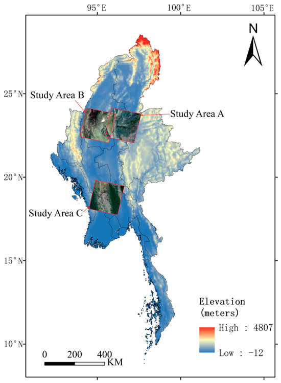
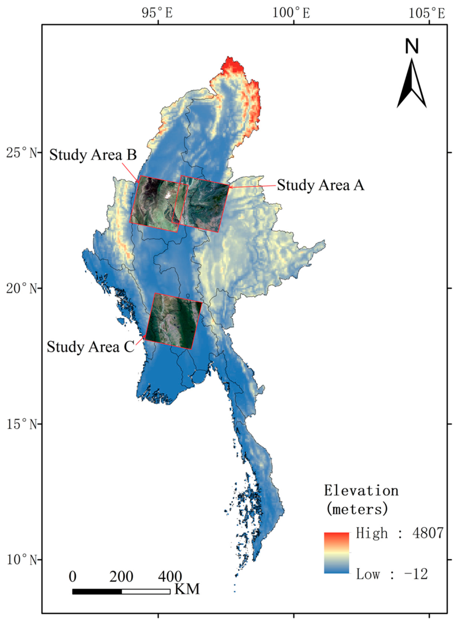
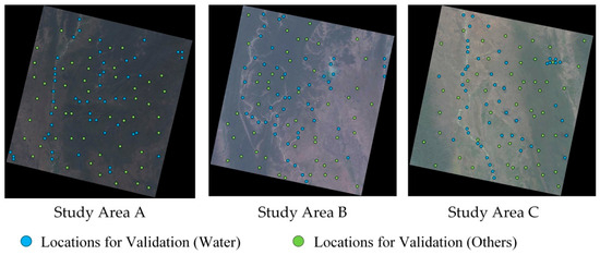
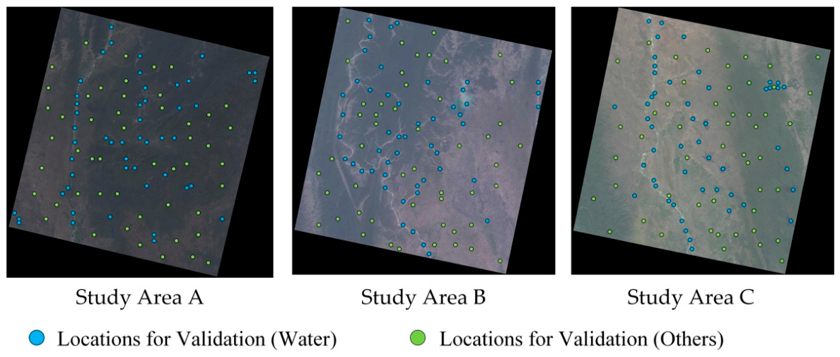
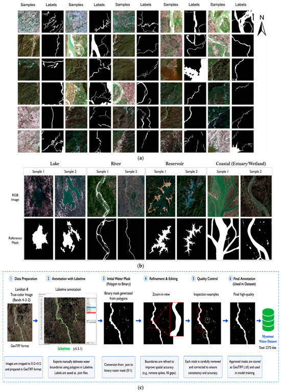
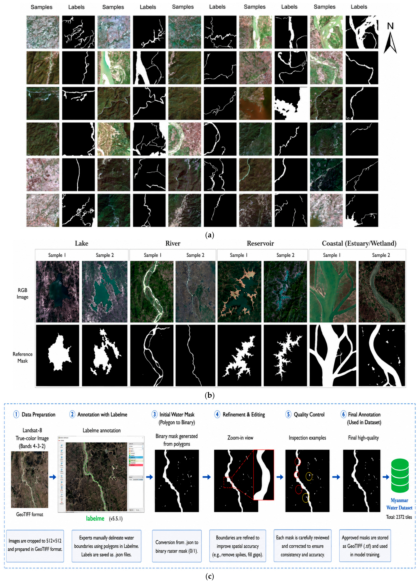
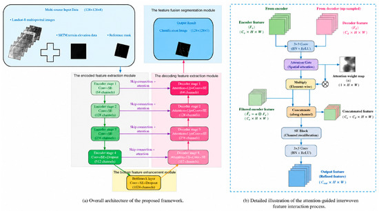
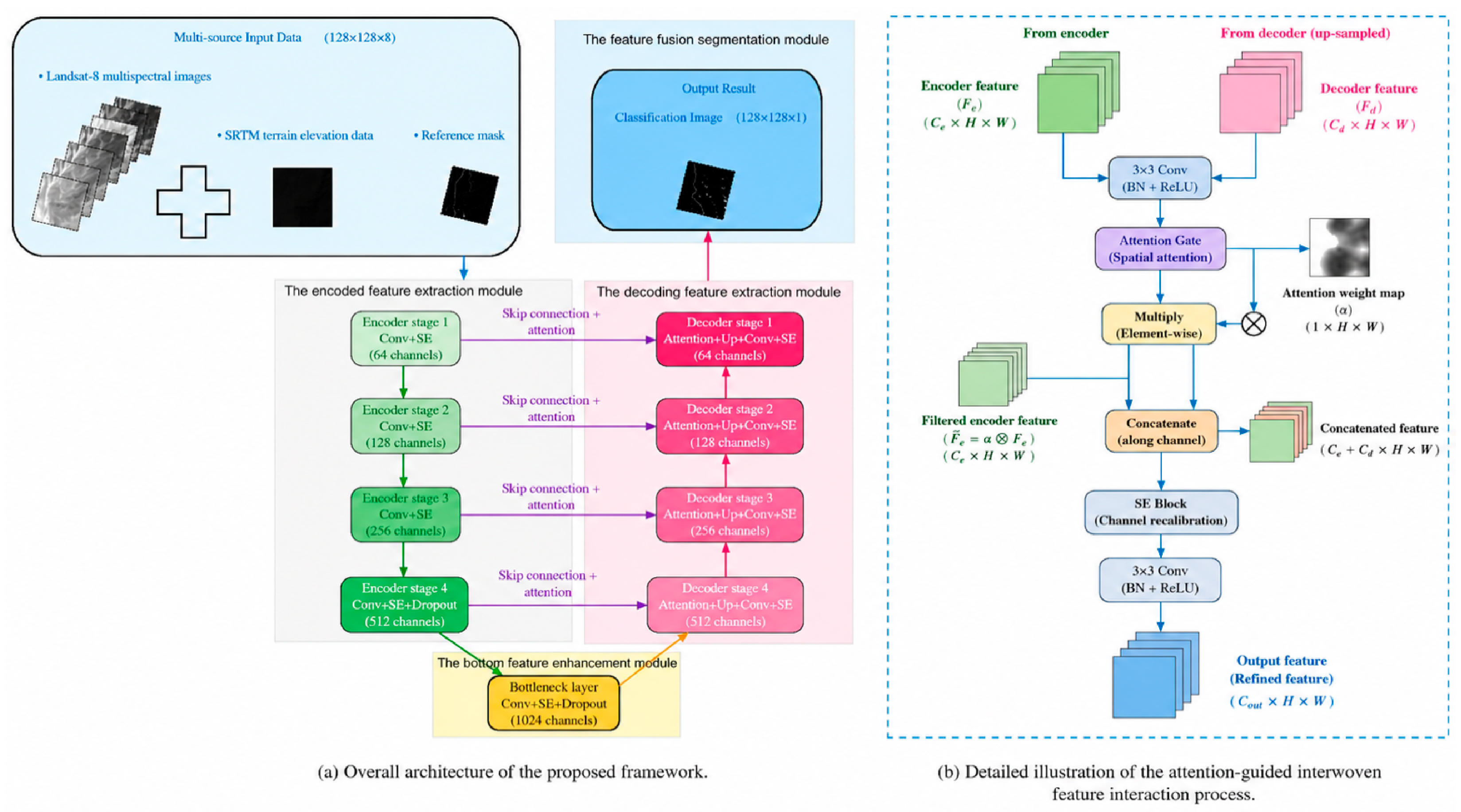
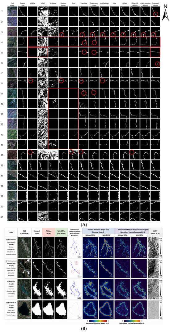
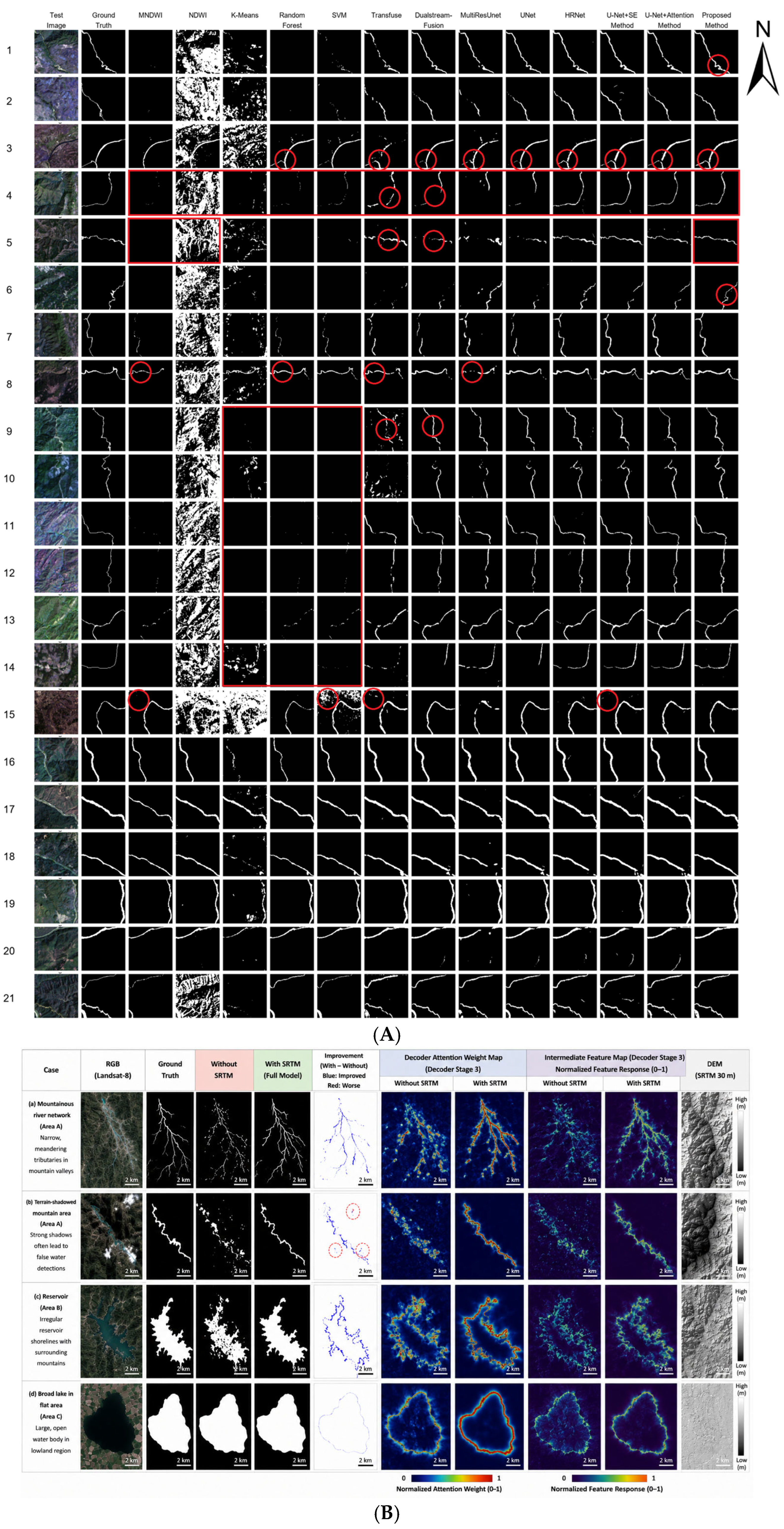
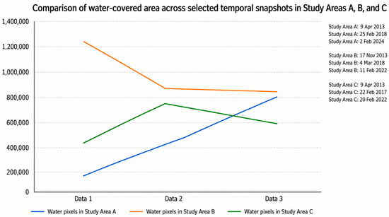
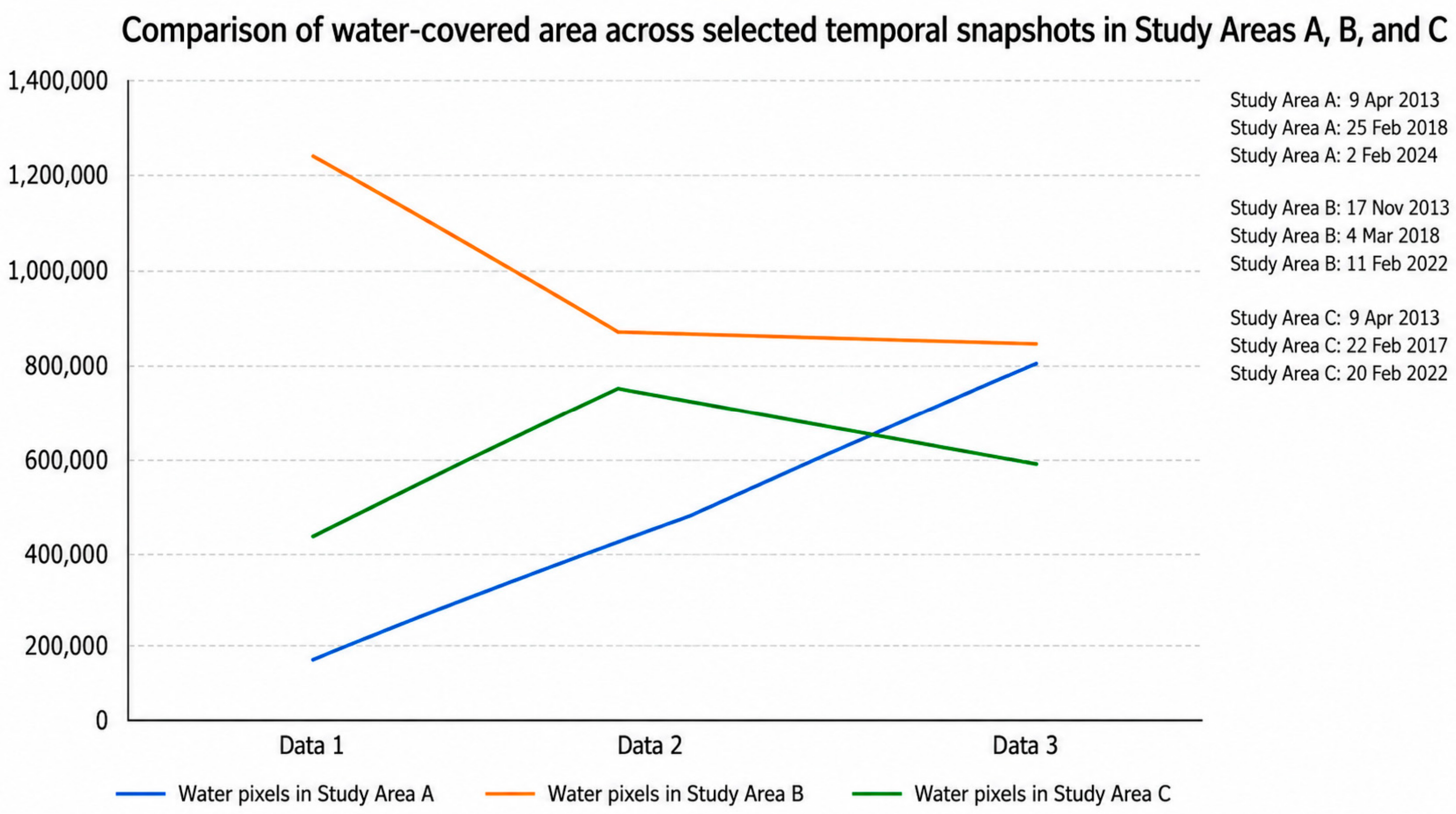
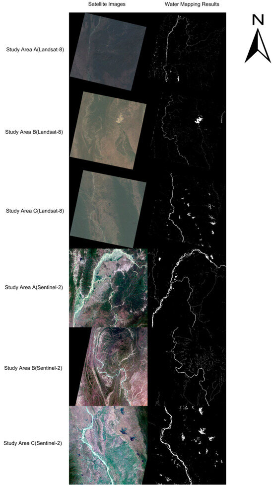
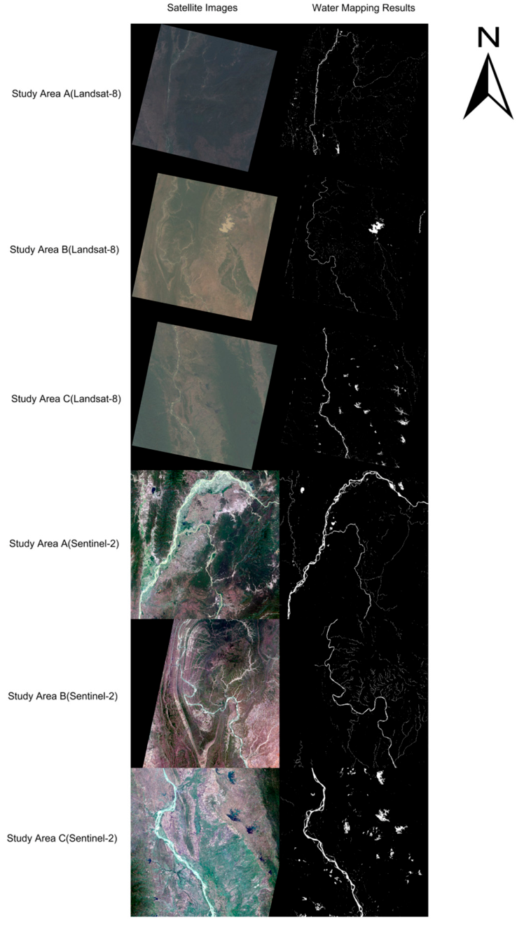
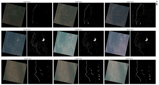
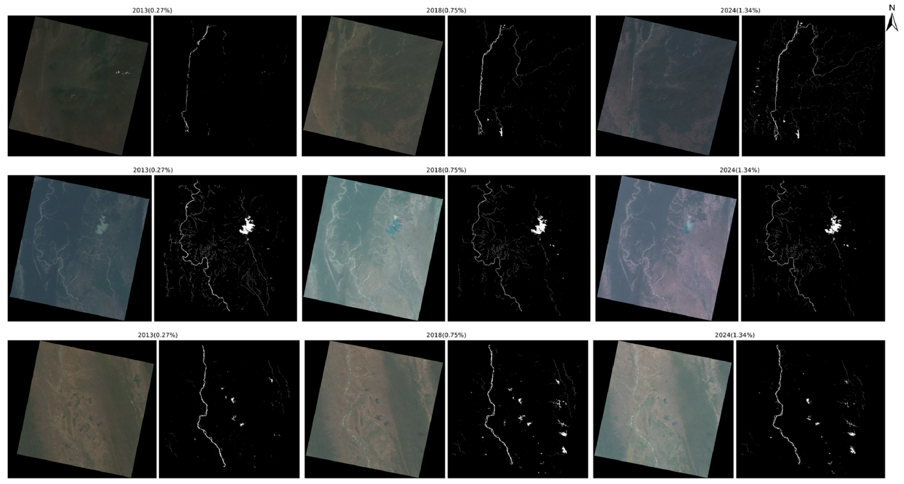
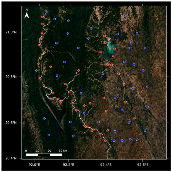
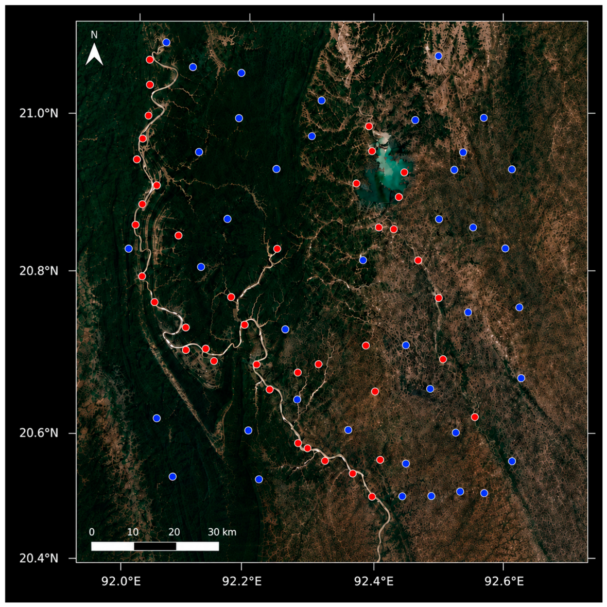

Disclaimer/Publisher’s Note: The statements, opinions and data contained in all publications are solely those of the individual author(s) and contributor(s) and not of MDPI and/or the editor(s). MDPI and/or the editor(s) disclaim responsibility for any injury to people or property resulting from any ideas, methods, instructions or products referred to in the content. |
© 2026 by the authors. Licensee MDPI, Basel, Switzerland. This article is an open access article distributed under the terms and conditions of the Creative Commons Attribution (CC BY) license.