HarmonicFormer: Cross-Phase Harmonic Modeling for Efficient Long-Term Water Quality Forecasting

Abstract

Water quality time series exhibit multi-scale periodicities, including daily and weekly cycles, driven by solar radiation, tidal forcing, and seasonal variation. Existing deep learning methods typically rely on patch-based attention or adaptive period decomposition, which suffer from parameter redundancy and high computational cost while failing to explicitly align with physical periodicities. To address this challenge, we propose HarmonicFormer, which restructures sequences into phase-period matrices, explicitly injects multi-scale periodic priors via harmonic temporal encoding, and achieves linear-complexity interactions through a lightweight cross-phase routing mechanism. Evaluated on hourly data from 37 monitoring stations in the Pearl River Basin (2020–2026) across nine water quality parameters and six forecast horizons, HarmonicFormer achieves the lowest average MSE of 0.3809 and MAE of 0.3753 over 54 experimental configurations, while maintaining high training efficiency and significantly reducing long-term error accumulation. Ablation studies confirm the effectiveness of harmonic encoding, reversible instance normalization, and key hyperparameters. This work offers an efficient and reliable explicit-periodicity modeling approach for water quality forecasting in the Pearl River Basin. Although the model currently adopts a fixed period length, future work can further enhance its generalization capability by introducing adaptive period discovery mechanisms.

1. Introduction

River water quality is central to ecosystem health and water security, yet global degradation has emerged as a prominent issue under the compounded pressures of climate change and human activity. Climate extremes are profoundly reshaping land-river connectivity, altering the physical, chemical, and biological composition of inland waters and directly affecting water availability assessments [1]. As China’s second-largest river system, the Pearl River has faced significant water quality deterioration over the past decade due to rapid urbanization, agricultural expansion, and socioeconomic disparities between upstream and downstream regions [2]. Comprehensive water quality index assessment methods [3] reveal significant spatiotemporal heterogeneity in key indicators such as total phosphorus and ammonia nitrogen within the Pearl River basin, with some areas falling into lower quality classes [2]. Accurate prediction of water quality dynamics is essential for resource management and risk mitigation, yet multiple challenges persist. Water chemistry encompasses thousands of variables governed by complex interactive processes [4]. More critically, water quality data are far sparser than hydrological data: global temporal coverage for total suspended solids is approximately 1%, compared to over 84% for streamflow [4]. Traditional statistical methods and process-based models struggle to capture nonlinear relationships in water quality dynamics, particularly under extreme conditions [4,5]. Deep learning offers new opportunities to address these challenges by leveraging multi-source data to fill spatiotemporal gaps and reveal complex patterns in high-dimensional datasets [4,5]. However, its application to river water quality prediction still faces challenges in capturing complex temporal dependencies, particularly the multi-scale periodic patterns inherent in water quality time series.

Summing up, below we enumerate the following challenges or limitations of existing methods:

1.

Traditional statistical models such as ARIMA and Prophet assume linearity and stationarity, failing to capture nonlinear and complex seasonal fluctuations in water quality dynamics. Conventional machine learning methods including SVR, Random Forest, and XGBoost remain heavily dependent on manual feature engineering and have limited capacity for high-dimensional, long-sequence data.

2.

Deep learning models like LSTM and CNN-based hybrid architectures have achieved promising results, but adaptively capturing key information from long sequences remains challenging.

3.

Periodicity-aware methods, including frequency-domain approaches like FreqCycle, adaptive period discovery methods such as TimesNet, and phase-based methods like PhaseFormer, still face limitations including global implicit representations, inaccurate decomposition under noise, and lack of explicit multi-scale periodic modeling mechanisms.

To address these challenges, this paper proposes HarmonicFormer, a model that improves prediction performance by explicitly modeling multi-scale periodic features in water quality data. The model adopts a phase-based representation paradigm, reorganizing time series into phase-period matrices where each phase token extracts observations at the same offset position across periods. This representation provides stronger global stationarity and lower feature dimensionality. Building on this foundation, HarmonicFormer innovatively introduces a harmonic temporal encoding mechanism that explicitly embeds periodic priors at different time scales through multi-period sinusoidal functions, enabling the model to simultaneously capture periodic variation patterns of water quality parameters across multiple time scales and effectively incorporating physical-ecological processes in water quality data. Additionally, the model employs a lightweight cross-phase routing mechanism that achieves efficient cross-phase dependency modeling through two-stage attention, avoiding the quadratic complexity of full attention mechanisms. This framework specifically addresses the limitations of existing methods in explicit multi-scale periodic modeling. The main contributions of this paper include:

1.

Based on multi-site water quality monitoring data from the Pearl River basin, we systematically analyzed the multi-scale periodic characteristics of parameters such as dissolved oxygen, pH, and ammonia nitrogen, providing a data foundation for explicit periodic modeling.

2.

We proposed the HarmonicFormer model, which explicitly embeds multi-scale prior knowledge such as diurnal and seasonal cycles through harmonic temporal encoding, achieving efficient modeling of inherent periodic structures in water quality data.

3.

We conducted extensive experiments on long-term prediction tasks for multiple water quality parameters. Results demonstrate that HarmonicFormer achieves optimal or near-optimal prediction performance across most water quality parameters and prediction horizons with extremely low parameter count and training cost, validating the effectiveness of explicit multi-scale periodic modeling in improving water quality prediction accuracy.

2. Related Work

Early water quality prediction research primarily relied on statistical time series models such as ARIMA and Prophet, which assume linearity and stationarity. These approaches struggle to capture nonlinear and complex seasonal fluctuations in water quality dynamics, and exhibit poor robustness to missing data and extreme events. Subsequently, machine learning methods such as SVR, Random Forest, and XGBoost were introduced. While these methods can capture nonlinear relationships to some extent, they remain heavily dependent on manual feature engineering and have limited capacity for high-dimensional, long-sequence data.

The rise of deep learning brought breakthrough progress to water quality prediction. Long short-term memory networks, as an improved recurrent neural network architecture, effectively addressed the vanishing gradient problem through gating mechanisms and cell states, enabling the capture of long-term temporal dependencies [6]. LSTM has demonstrated strong capability in water quality prediction, with confirmed higher prediction accuracy and robustness compared to traditional machine learning methods in inland water quality modeling [7]. In practical applications, deep LSTM networks combined with Pearson correlation coefficient analysis to identify parameter associations have successfully achieved high-precision short-term and long-term prediction of pH and water temperature in marine aquaculture [8]. Gated recurrent units, as a simplified LSTM variant, reduced computational complexity by decreasing the number of gating units [9]. The proposal of sequence-to-sequence learning frameworks further expanded deep learning applications in sequence modeling, enabling end-to-end learning of variable-length sequences through encoder-decoder structures [10]. However, standalone LSTM models struggle to avoid noise interference and can only perform unidirectional prediction based on historical information. Researchers therefore began exploring hybrid architectures. Convolutional neural networks were introduced to temporal modeling for their strong local feature extraction capability. Temporal convolutional networks demonstrated superior performance to LSTM and longer effective memory in multiple sequence modeling tasks [11]. Building on this foundation, hybrid models integrating ensemble empirical mode decomposition with CNN-BiLSTM were proposed. These models eliminate noise influence through EEMD decomposition, extract local features via CNN, and leverage BiLSTM to simultaneously consider forward and backward temporal dependencies, thereby effectively improving dissolved oxygen prediction performance [12]. The success of these hybrid architectures indicates that combining the strengths of different deep learning techniques can more effectively address the complex characteristics of water quality data.

Although hybrid architectures combining LSTM and CNN significantly improved water quality prediction performance, adaptively capturing key information from long-sequence data remains challenging. The attention mechanism provided a new solution to this problem. By automatically searching for parts of the source sequence relevant to target prediction, attention mechanisms effectively addressed the information bottleneck of fixed-length vectors in encoder-decoder architectures [13]. In water quality prediction, attention mechanisms were combined with LSTM to enhance the influence of key features by assigning differentiated weights to sequences at different time steps, successfully achieving single-step and multi-step prediction of dissolved oxygen in the Burnett River, Australia [14]. Building on this, LSTM models based on multi-head attention were further proposed to capture multi-faceted temporal relationships in water quality data through multi-head mechanisms, improving prediction performance by approximately 5% to 8% compared to existing models on Irish water quality datasets [15].

Building on attention mechanisms, the proposal of the Transformer architecture changed the sequence modeling paradigm. It abandoned recurrent structures and relied solely on self-attention mechanisms to capture global dependencies, achieving remarkable success in natural language processing and other fields [16]. However, directly applying it to long-sequence time series prediction faces two major challenges: first, the time and memory complexity of self-attention mechanisms grows quadratically with sequence length, limiting input sequence length; second, point-wise attention struggles to effectively extract local semantic information from time series. Addressing the complexity problem, researchers proposed improvements from different angles. Informer introduced a probabilistic sparse self-attention mechanism to select important query-key pairs, reducing complexity to log-linear level, and adopted a generative decoder to achieve one-step prediction of long sequences [17]. Autoformer incorporated series decomposition as an internal module and designed an auto-correlation mechanism leveraging series periodicity to perform dependency discovery and aggregation at the sub-series level, also achieving logarithmic complexity [18]. For the local semantic information deficiency, PatchTST segmented time series into sub-sequence-level patches as input tokens, preserving local information while dramatically reducing computational cost, and adopted a channel-independent strategy to avoid noise interference between multiple variables [19]. Building on this foundation, iTransformer further reconstructed the responsibility allocation of Transformer modules by inverting the operational dimension, applying attention mechanisms to the variable dimension to capture multivariate correlations while using feed-forward networks for independent time series representation learning for each variable [20]. In water quality prediction applications, STGFT, a long-term water quality prediction model based on spatiotemporal graph-fused Transformer, was proposed. It integrates a spatial attention encoder, temporal attention encoder, and adaptive dynamic adjacency matrix generator to separately capture spatial correlations and temporal features across different monitoring stations, and reflects latent spatial relationships in river networks by generating adaptive and dynamic graphs [5]. These Transformer-based methods demonstrated powerful long-range dependency modeling capability, providing new technical pathways for water quality prediction.

Beyond temporal dependencies, spatial relationships among water quality monitoring stations also affect prediction performance. Graph neural networks have been widely applied to spatiotemporal sequence prediction due to their capability to process non-Euclidean data. Graph convolutional networks effectively capture local structure and features among nodes by performing convolution operations directly on graph structures [21]. Graph attention networks were further proposed to assign different weights to neighboring nodes through attention mechanisms, enhancing model expressiveness [22]. Spatiotemporal graph convolutional network STGCN combined graph convolution with temporal convolution, demonstrating the capability to simultaneously model spatial and temporal dependencies in traffic flow prediction [23]. In the water quality prediction domain, temporal-relational graph neural networks extracted parameter correlations through weighted adjacency matrices, achieving multivariate multi-step prediction of coastal seawater quality parameters [24]. For plain river networks, spatiotemporal graph neural network ST-GNN was proposed, integrating adaptive multi-period enhancement and temporal periodic dependency modules to capture complex spatiotemporal dependencies [25]. However, GNN methods have limitations in river water quality prediction: Pearl River basin water quality data exhibits unidirectional flow characteristics, with highly sparse adjacency matrices between upstream and downstream stations, limiting GNN effectiveness in capturing complex spatial dependencies.

Many real-world time series exhibit clear periodic or quasi-periodic structures, such as urban traffic flow, electricity and gas loads, cloud and data center resource utilization, and network traffic. The water quality data used in this study are influenced by multiple factors including seasonal variations, tidal cycles, and human activities, also exhibiting significant periodic patterns. Beyond spatiotemporal dependencies, these inherent periodic features are critical to prediction performance. Targeting this characteristic, researchers proposed a series of methods from frequency-domain analysis and multi-period modeling perspectives. FEDformer embedded seasonal-trend decomposition into Transformer, leveraging Fourier transform to capture sparse representations in the frequency domain to extract global characteristics [26]. Pyraformer constructed a multi-resolution tree structure through pyramid attention modules, aggregating global features via cross-scale connections and modeling local dependencies through same-scale adjacency relationships [27]. TimesNet further decomposed complex variations into intra-period and inter-period categories, converting one-dimensional sequences into two-dimensional tensors to enable convolutional kernels to simultaneously capture both types of variations [28]. These methods were subsequently introduced to the water quality prediction domain. Temporal Fusion Transformer was used to integrate features across different time scales, achieving modeling and prediction of river water quality indices [29]. An ensemble model integrating Informer, Autoformer, and FEDformer also achieved excellent performance in wastewater treatment plant water quality parameter prediction [30]. These methods provided new technical pathways for water quality prediction.

Empirical studies demonstrate that river water quality data exhibit significant multi-timescale periodic patterns. Through continuous monitoring of the tidal freshwater zone in the Potomac River, water temperature, dissolved oxygen, and pH showed strong and consistent diurnal cycles under stable conditions, while conductivity exhibited semi-diurnal cycles. These periodic patterns are influenced by seasonal variations in driving factors such as light, tides, and freshwater inflow [31]. Spatiotemporal variation assessments of the middle and lower reaches of the Han River revealed significant seasonal variation patterns in water quality parameters, with the lowest water quality indices occurring in summer and autumn [32]. In studies of the Xijiang River basin, correlations between water quality parameters and meteorological factors were further confirmed, with the temperature-dissolved oxygen relationship indicating that meteorological influences must be incorporated into water quality prediction processes [33]. These studies collectively demonstrate that water quality data simultaneously contain multi-scale periodic features such as diurnal and seasonal cycles, and that these cycles are driven by physical-ecological processes including light, temperature, and human activities.

While several periodicity-aware forecasting methods have been developed—including frequency-domain approaches such as FreqCycle [34], adaptive period discovery methods such as TimesNet [28], and phase-based methods such as PhaseFormer [35]—they still face limitations in explicitly modeling the multi-scale periodicities inherent in water quality data. Overall, existing approaches lack explicit mechanisms for capturing multiple periodic scales simultaneously, motivating the need for a more effective solution.

3. Method

This paper focuses on forecasting tasks for multivariate time series. Given a historical observation sequence $\mathit{X}=\{{\mathit{x}}_1,{\mathit{x}}_2,\dots ,{\mathit{x}}_{L_{\mathrm{in}}}\}\in {\mathbb{R}}^{L_{\mathrm{in}}\times C}$, the model predicts the future sequence $\mathit{Y}=\{{\mathit{y}}_1,{\mathit{y}}_2,\dots ,{\mathit{y}}_{L_{\mathrm{out}}}\}\in {\mathbb{R}}^{L_{\mathrm{out}}\times C}$ for $L_{\mathrm{out}}$ time steps. Due to significant differences in physical meaning and variation patterns among different water quality parameters, this paper adopts the channel-independent paradigm [19,36], training separate models for different water quality parameters without sharing parameters. In the spatial dimension, the model input consists of historical data from 37 monitoring stations, with output being future data for these stations. Subsequent descriptions use a single parameter as an example, with multivariate cases independently generalizable.

Water quality time series exhibit significant multi-scale periodic characteristics. Setting the fundamental period length as $L_{\mathrm{phase}}$, such as 24 for hourly data corresponding to diurnal cycles, the number of periods contained in the input sequence $P_{\mathrm{in}}$ and the number of periods in the output sequence $P_{\mathrm{out}}$ are respectively:

$$P_{\mathrm{in}}=\lceil L_{\mathrm{in}}/L_{\mathrm{phase}}\rceil P_{\mathrm{out}}=\lceil L_{\mathrm{out}}/L_{\mathrm{phase}}\rceil$$

(1)

The core idea of HarmonicFormer is to improve water quality prediction accuracy by explicitly modeling these multi-scale periodic features.

3.1. Data Preprocessing

Water quality parameters have significantly different dimensions and value ranges. To eliminate the influence of different parameter dimensions and accelerate model convergence, this paper adopts Reversible Instance Normalization [37] to normalize the input sequence. Unlike conventional normalization methods that rely on global statistics, RevIN normalizes each input instance independently using its own mean and standard deviation. This instance-wise strategy avoids the distribution mismatch problem between training and test sets, and enhances robustness against non-stationarity and outliers in water quality time series. Its reversible design further ensures that predictions can be accurately restored to the original scale. Given an input sequence $\mathit{x}\in {\mathbb{R}}^{L_{\mathrm{in}}}$, the mean and standard deviation are first calculated:

$$\mu ={\displaystyle \frac{1}{L_{\mathrm{in}}}}{\displaystyle \sum _{t=1}^{L_{\mathrm{in}}}}{x}_t\sigma =\sqrt{{\displaystyle \frac{1}{L_{\mathrm{in}}}}\sum _{t=1}^{L_{\mathrm{in}}}{(x_t-\mu )}^2+ϵ}$$

(2)

The normalized sequence is $\tilde{\mathit{x}}={\displaystyle \frac{\mathit{x}-\mu }{\sigma }}$. The model performs prediction on the normalized sequence, obtaining the normalized prediction result $\tilde{\mathit{y}}$. In the output stage, the original dimension is recovered through denormalization:

$$\mathit{y}=\tilde{\mathit{y}}·\sigma +\mu$$

(3)

After RevIN normalization, the model adopts Phase Tokenization to reorganize the one-dimensional time series into a two-dimensional phase-period matrix, explicitly modeling the periodic characteristics of water quality data. Setting the fundamental period length as $L_{\mathrm{phase}}$ and the input sequence length as $L_{\mathrm{in}}$, to ensure the sequence length is an integer multiple of the period length, the input sequence is first cyclically padded to length $P_{\mathrm{in}}\times L_{\mathrm{phase}}$, where $P_{\mathrm{in}}=\lceil L_{\mathrm{in}}/L_{\mathrm{phase}}\rceil$ is the number of periods contained in the input. The padded sequence ${\mathit{x}}_{\mathrm{pad}}\in {\mathbb{R}}^{P_{\mathrm{in}}\times L_{\mathrm{phase}}}$ is reorganized into a phase-period matrix according to the following formula:

$${\mathit{X}}_{\mathrm{phase}}[\ell ,p]={\mathit{x}}_{\mathrm{pad}}[(p-1)·L_{\mathrm{phase}}+\ell ]$$

(4)

where $\ell \in \{1,\dots ,L_{\mathrm{phase}}\}$ is the phase index and $p\in \{1,\dots ,P_{\mathrm{in}}\}$ is the period index. Each row phase token of this matrix contains observations at the same phase across multiple periods. Phase tokens possess stronger global stationarity and lower feature dimensionality [35], providing an efficient representational foundation for subsequent periodic modeling.

In the prediction stage, the model outputs a phase-period matrix ${\mathit{Y}}_{\mathrm{phase}}\in {\mathbb{R}}^{L_{\mathrm{phase}}·P_{\mathrm{out}}}$ or ${\mathit{Y}}_{\mathrm{phase}}\in {\mathbb{R}}^{C·L_{\mathrm{phase}}·P_{\mathrm{out}}}$ in the multivariate case. This is reorganized into a one-dimensional prediction sequence $\mathit{y}\in {\mathbb{R}}^{L_{\mathrm{out}}}$ through phase detokenization, completing the mapping from phase space to temporal space.

3.2. HarmonicFormer Model

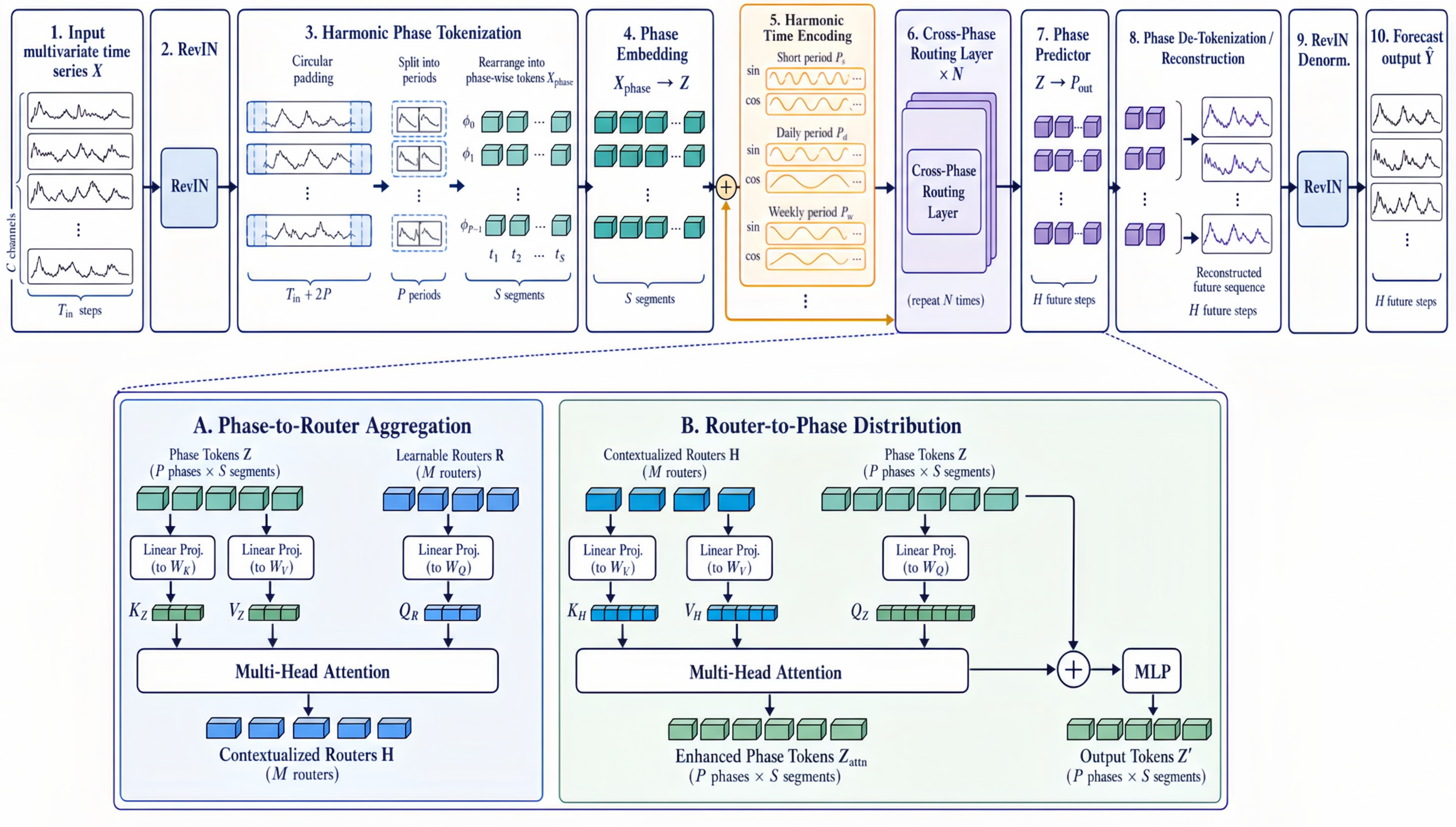
The overall architecture of HarmonicFormer is shown in Figure 1. The model adopts an encoder-predictor structure, mainly comprising a phase embedding layer, harmonic temporal encoding, cross-phase routing layers, and a predictor. Given the preprocessed phase-period matrix ${\mathit{X}}_{\mathrm{phase}}\in {\mathbb{R}}^{C\times L_{\mathrm{phase}}\times P_{\mathrm{in}}}$, the model first maps it to the latent space through the phase embedding layer, subsequently introduces harmonic temporal encoding to explicitly embed multi-scale periodic priors, then performs feature interaction and extraction through multiple cross-phase routing layers, and finally generates predictions for the future $P_{\mathrm{out}}$ periods through the predictor.

3.2.1. Harmonic Time Encoding

Harmonic time encoding aims to explicitly model multi-scale periodic features driven by physical-ecological processes in water quality data. Water quality parameters are influenced by factors such as light, temperature, and human activities, exhibiting periodic variation patterns at multiple time scales including diurnal and weekly cycles. To capture these inherent periodicities, this paper designs a harmonic time encoding mechanism based on multi-period sinusoidal functions.

For a phase sequence with period length $L_{\mathrm{phase}}$, a set of periods $\mathcal{P}=\{p_1,p_2,\dots ,p_k\}$ is defined. This paper sets $\mathcal{P}=\{1,L_{\mathrm{phase}},7·L_{\mathrm{phase}}\}$, where $p=1$ corresponds to capturing fundamental high-frequency fluctuations, $p=L_{\mathrm{phase}}$ corresponds to diurnal cycle patterns driven by factors such as light and temperature, and $p=7·L_{\mathrm{phase}}$ corresponds to weekly cycle patterns driven by factors such as human activities. For each period $p_k$, cosine and sine encodings are generated at phase index $\ell \in \{0,1,\dots ,L_{\mathrm{phase}}-1\}$:

$$cos\left({\displaystyle \frac{2\pi \ell }{p_k}}\right)sin\left({\displaystyle \frac{2\pi \ell }{p_k}}\right)$$

(5)

Concatenating the sine and cosine encodings of all periods yields a $2k$-dimensional harmonic feature vector:

$${\mathit{h}}_{\ell }={\left[cos\left({\displaystyle \frac{2\pi \ell }{p_1}}\right),sin\left({\displaystyle \frac{2\pi \ell }{p_1}}\right),\dots ,cos\left({\displaystyle \frac{2\pi \ell }{p_k}}\right),sin\left({\displaystyle \frac{2\pi \ell }{p_k}}\right)\right]}^T\in {\mathbb{R}}^{2k}$$

(6)

Subsequently, a linear projection layer maps the harmonic features to the model’s latent dimension d:

$${\mathit{e}}_{\ell }={\mathit{W}}_h{\mathit{h}}_{\ell }\in {\mathbb{R}}^d$$

(7)

where ${\mathit{W}}_h\in {\mathbb{R}}^{d\times 2k}$ is a learnable projection matrix. The encoding vectors of all phases form the harmonic time encoding matrix:

$${\mathit{E}}_{\mathrm{time}}={[{\mathit{e}}_0,{\mathit{e}}_1,\dots ,{\mathit{e}}_{L_{\mathrm{phase}}-1}]}^T\in {\mathbb{R}}^{L_{\mathrm{phase}}\times d}$$

(8)

Finally, the harmonic time encoding is added to the phase embeddings, explicitly injecting multi-scale periodic prior knowledge into the model.

3.2.2. Phase Embedding

The phase embedding layer is responsible for mapping the phase-period matrix ${\mathit{X}}_{\mathrm{phase}}\in {\mathbb{R}}^{C\times L_{\mathrm{phase}}\times P_{\mathrm{in}}}$ to the model’s latent representation space. For each phase $\ell \in \{1,\dots ,L_{\mathrm{phase}}\}$, the corresponding phase token is a column vector:

$${\mathit{x}}_{\ell }={[{\mathit{X}}_{\mathrm{phase}}[\ell ,1],{\mathit{X}}_{\mathrm{phase}}[\ell ,2],\dots ,{\mathit{X}}_{\mathrm{phase}}[\ell ,P_{\mathrm{in}}]]}^T\in {\mathbb{R}}^{P_{\mathrm{in}}}$$

(9)

The phase embedding layer maps the phase token to the d-dimensional latent space through linear transformation:

$${\mathit{z}}_{\ell }={\mathit{W}}_e{\mathit{x}}_{\ell }\in {\mathbb{R}}^d$$

(10)

where ${\mathit{W}}_e\in {\mathbb{R}}^{d\times P_{\mathrm{in}}}$ is a learnable embedding matrix. Stacking the embedding vectors of all phases yields the phase embedding matrix:

$$\mathit{Z}={[{\mathit{z}}_1,{\mathit{z}}_2,\dots ,{\mathit{z}}_{L_{\mathrm{phase}}}]}^T\in {\mathbb{R}}^{L_{\mathrm{phase}}\times d}$$

(11)

Subsequently, the harmonic time encoding ${\mathit{E}}_{\mathrm{time}}$ is added to the phase embedding $\mathit{Z}$, obtaining a phase representation that incorporates periodic priors:

$$\tilde{\mathit{Z}}=\mathit{Z}+{\mathit{E}}_{\mathrm{time}}$$

(12)

This representation serves as the input to subsequent cross-phase routing layers.

3.2.3. Cross-Phase Routing Layer

The cross-phase routing layer is responsible for modeling dependencies between different phases and capturing cross-period temporal dynamic features. Directly applying full attention across all phases would yield time complexity of $O\left(L_{\mathrm{phase}}^2\right)$, which incurs significant computational overhead when the period length is large. To improve efficiency, this paper introduces a two-stage attention mechanism based on routers [35]. Specifically, K learnable routers are set:

$$\mathit{R}={[{\mathit{r}}_1,{\mathit{r}}_2,\dots ,{\mathit{r}}_K]}^T\in {\mathbb{R}}^{K\times d}$$

(13)

serving as intermediaries for information exchange. First, phase-to-router aggregation is performed, using routers as queries and phase representations as keys and values, aggregating phase information through multi-head attention:

$$\mathit{H}=\mathrm{MultiHeadAttn}({\mathit{Q}}_r,{\mathit{K}}_z,{\mathit{V}}_z)$$

(14)

where ${\mathit{Q}}_z=\tilde{\mathit{Z}}{\mathit{W}}_Q^{\mathrm{dist}}$, ${\mathit{K}}_r=\mathit{H}{\mathit{W}}_K^{\mathrm{dist}}$, ${\mathit{V}}_r=\mathit{H}{\mathit{W}}_V^{\mathrm{dist}}$. Finally, residual connections, layer normalization, and feed-forward networks are applied for further processing:

$${\mathit{Z}}^{\prime }=\mathrm{LayerNorm}(\tilde{\mathit{Z}}+\mathrm{Dropout}\left({\mathit{Z}}_{\mathrm{attn}}\right))$$

(15)

$${\mathit{Z}}_{\mathrm{out}}=\mathrm{LayerNorm}({\mathit{Z}}^{\prime }+\mathrm{Dropout}\left(\mathrm{FFN}\left({\mathit{Z}}^{\prime }\right)\right))$$

(16)

where FFN consists of two linear transformations and a GELU activation function. The model stacks N cross-phase routing layers to progressively extract higher-level feature representations. Through the router mechanism, time complexity is reduced to $\mathcal{O}(L_{\mathrm{phase}}·K·d)$.

3.2.4. Phase Predictor

After processing through multiple cross-phase routing layers, the model obtains phase representations ${\mathit{Z}}^{\left(L\right)}\in {\mathbb{R}}^{C\times L_{\mathrm{phase}}\times d}$ that integrate multi-scale periodic information. The predictor module employs linear projection to map each phase token from latent dimension d to the output period count $P_{\mathrm{out}}$:

$${\mathit{Y}}_{\mathrm{phase}}={\mathit{Z}}^{\left(L\right)}{\mathit{W}}_{\mathrm{pred}}+{\mathit{b}}_{\mathrm{pred}}$$

(17)

where ${\mathit{W}}_{\mathrm{pred}}\in {\mathbb{R}}^{d\times P_{\mathrm{out}}}$ and ${\mathit{b}}_{\mathrm{pred}}\in {\mathbb{R}}^{P_{\mathrm{out}}}$ are learnable parameters, and ${\mathit{Y}}_{\mathrm{phase}}\in {\mathbb{R}}^{B\times C\times L_{\mathrm{phase}}\times P_{\mathrm{out}}}$ is the prediction result in phase space.

3.2.5. Phase Detokenization

The phase-period matrix ${\mathit{Y}}_{\mathrm{phase}}\in {\mathbb{R}}^{B\times C\times L_{\mathrm{phase}}\times P_{\mathrm{out}}}$ output by the predictor needs to be converted back to time series form through phase detokenization, which is the inverse operation of phase tokenization. First, the phase-period matrix is reorganized into a period-phase matrix through dimension permutation:

$${\mathit{Y}}_{\mathrm{periods}}=\mathrm{Permute}({\mathit{Y}}_{\mathrm{phase}},[0,1,3,2])$$

(18)

yielding ${\mathit{Y}}_{\mathrm{periods}}\in {\mathbb{R}}^{B\times C\times P_{\mathrm{out}}\times L_{\mathrm{phase}}}$. Subsequently, the period dimension and phase dimension are flattened into a continuous time series:

$${\mathit{Y}}_{\mathrm{flat}}=\mathrm{Reshape}({\mathit{Y}}_{\mathrm{periods}},[B,C,P_{\mathrm{out}}\times L_{\mathrm{phase}}])$$

(19)

Since period alignment may generate redundant time steps, the target prediction length is truncated:

$$\widehat{\mathit{Y}}={\mathit{Y}}_{\mathrm{flat}}[\cdots ,\cdots ,L_{\mathrm{pred}}]$$

(20)

where $L_{\mathrm{pred}}=L_{\mathrm{out}}$ is the prediction sequence length. Finally, the standard time series format is restored through dimension permutation:

$$\widehat{\mathit{Y}}\in {\mathbb{R}}^{B\times C\times L_{\mathrm{pred}}}$$

(21)

Then the original scale is recovered through RevIN denormalization:

$${\mathit{y}}_{\mathrm{final}}=\widehat{\mathit{y}}\odot \sigma +\mu$$

(22)

where $\mu$ and $\sigma$ are the statistics saved during input sequence normalization, and ⊙ denotes element-wise multiplication.

3.3. Model Complexity Analysis

The computational complexity of HarmonicFormer primarily consists of three components: the phase embedding layer, cross-phase routing layers, and the predictor. In the phase embedding layer, for each variable’s phase sequence ${\mathit{X}}_{\mathrm{phase}}\in {\mathbb{R}}^{L_{\mathrm{phase}}\times P_{\mathrm{in}}}$, the linear projection has complexity $\mathcal{O}(C·L_{\mathrm{phase}}·P_{\mathrm{in}}·d)$. Since $P_{\mathrm{in}}=\lceil L_{\mathrm{in}}/L_{\mathrm{phase}}\rceil$ is typically small, the computational overhead of this component is limited.

Each cross-phase routing layer contains a two-stage attention mechanism. In the phase-to-router aggregation stage, attention is computed between $L_{\mathrm{phase}}$ phase tokens and K router tokens, with complexity $\mathcal{O}(C·L_{\mathrm{phase}}·K·d)$. The router-to-phase distribution stage has identical complexity. Therefore, the total complexity of a single cross-phase routing layer is $\mathcal{O}(C·L_{\mathrm{phase}}·K·d)$. For L routing layers, the total complexity is:

$$\mathcal{O}(L·C·L_{\mathrm{phase}}·K·d)$$

(23)

By introducing a fixed number of router tokens as intermediaries, this mechanism avoids the $\mathcal{O}\left(L_{\mathrm{phase}}^2\right)$ complexity of full attention. Since the period length P, router count K, number of layers L, and feature dimension d are all fixed hyperparameters, the model’s computational cost grows linearly with input length $L_{\mathrm{in}}$ and output length $L_{\mathrm{out}}$. The linear projection of the predictor has complexity $\mathcal{O}(C·L_{\mathrm{phase}}·d·P_{\mathrm{out}})$. Synthesizing the above analysis, the overall time complexity of HarmonicFormer is:

$$\mathcal{O}(L·C·L_{\mathrm{phase}}·K·d)$$

(24)

Compared to the $\mathcal{O}(T^2·d)$ complexity of standard Transformer, this provides significant computational advantages when processing long sequences. Additionally, the phase-based representation reduces the feature dimension from T to $L_{\mathrm{phase}}$, further decreasing model parameter count and memory usage.

4. Dataset

The Pearl River is the largest river system in southern China, with a basin area of approximately $45.4\times {10}^4{km}^2$, formed by the confluence of three major water systems: the Xijiang, Beijiang, and Dongjiang. Located in the subtropical monsoon climate zone, the Pearl River basin receives abundant rainfall, with annual precipitation of 1500–2000 mm and runoff ranking second nationally after the Yangtze River. The basin is densely populated and economically developed, serving as a vital water source for the Guangdong-Hong Kong-Macao Greater Bay Area. Water quality directly affects regional ecological security and drinking water safety for tens of millions of residents.

The data used in this study were collected from 37 cross-section monitoring stations of the Pearl River basin automatic water quality monitoring system. These 37 stations are distributed across the river network of the Pearl River Delta, with the following administrative divisions: 14 stations in the Guangzhou section, located at 113°15′–113°40′ E, 22°50′–23°10′ N; 6 stations in the Foshan section, located at 113°00′–113°15′ E, 22°50′–23°05′ N; 10 stations in the Zhongshan section, located at 113°15′–113°30′ E, 22°25′–22°45′ N; and 7 stations in the Zhuhai section, located at 113°25′–113°40′ E, 22°05′–22°25′ N. The stations cover the complete hydrological propagation chain from upstream inputs to estuary discharge, distributed across major cities including Zhaoqing, Guangzhou, Foshan, Zhongshan, Jiangmen, and Zhuhai, encompassing the Xijiang and Beijiang main streams, their major tributaries, and estuarine channels such as Modaomen and Jitimen. The station layout fully considers basin hydrological connectivity, facilitating capture of pollutant migration and transformation processes within the basin. Stations in estuarine areas including Zhuhai, Jiangmen, and Zhongshan are located at river-sea convergence zones, subject to dual influences from Pearl River runoff and South China Sea tides. Complex hydrodynamic conditions exist with tidal backflow and saltwater intrusion phenomena, causing water quality parameters to exhibit semi-diurnal tidal periodic fluctuations, presenting unique challenges for water quality prediction.

Data from the Pearl River basin automatic water quality monitoring system span from April 2020 to April 2026, covering nearly six years. The dataset includes 37 monitoring stations with a sampling interval of 4 h, totaling 14,081 time steps, providing substantial sample support for water quality prediction. To facilitate parameter-independent modeling, we aggregated the raw data by water quality parameter and monitoring site, generating separate feature files for each of the nine water quality parameters, each with a unified spatiotemporal dimension for consistent model loading and processing. The overall missing rate of the dataset is 1.15%, which is relatively low; therefore, linear interpolation based on adjacent observations was applied for imputation. For outliers, we performed outlier detection using the Interquartile Range (IQR) method with a threshold of $3\times IQR$. Values exceeding $Q_1-3\times IQR$ or $Q_3+3\times IQR$ were flagged as potential outliers. To avoid gaps in the time series caused by sample removal and to mitigate the adverse effects of extreme values on model training, we adopted Winsorization to cap the detected outliers to the corresponding boundary values. In the dataset, approximately 2.14% of the observations were corrected, while the overall statistical characteristics of each feature remained largely unchanged before and after processing, indicating that this method effectively suppresses extreme outliers while preserving the original data distribution.

Monitoring parameters include nine indicators: water temperature, pH, dissolved oxygen, ammonia nitrogen, total nitrogen, total phosphorus, conductivity, permanganate index, and turbidity, covering the physical, chemical, and biological characteristics of water bodies.

Table 1. Statistical Summary of Water Quality Parameters.

Parameter	Unit	Mean	Std	Min	Max	Missing Rate (%)
Water Temperature	°C	24.389	4.792	0.000	38.260	0.23%
pH	–	7.493	0.551	4.050	10.670	0.37%
Dissolved Oxygen	mg/L	7.141	2.066	0.005	29.370	0.23%
Ammonia Nitrogen	mg/L	0.121	0.229	0.000	22.204	2.37%
Total Nitrogen	mg/L	2.449	1.027	0.000	48.382	2.09%
Total Phosphorus	mg/L	0.070	0.049	0.000	2.431	1.61%
Conductivity	μS/cm	1330.615	3433.925	0.001	37,565.110	1.67%
Permanganate Index	mg/L	2.768	1.747	0.000	47.054	1.51%
Turbidity	NTU	42.753	86.154	0.001	8934.345	0.31%

lists the statistical characteristics of each parameter across the entire dataset, including mean, standard deviation, minimum, maximum, and missing rate. The overall missing rates are low, indicating stable and reliable monitoring system operation.

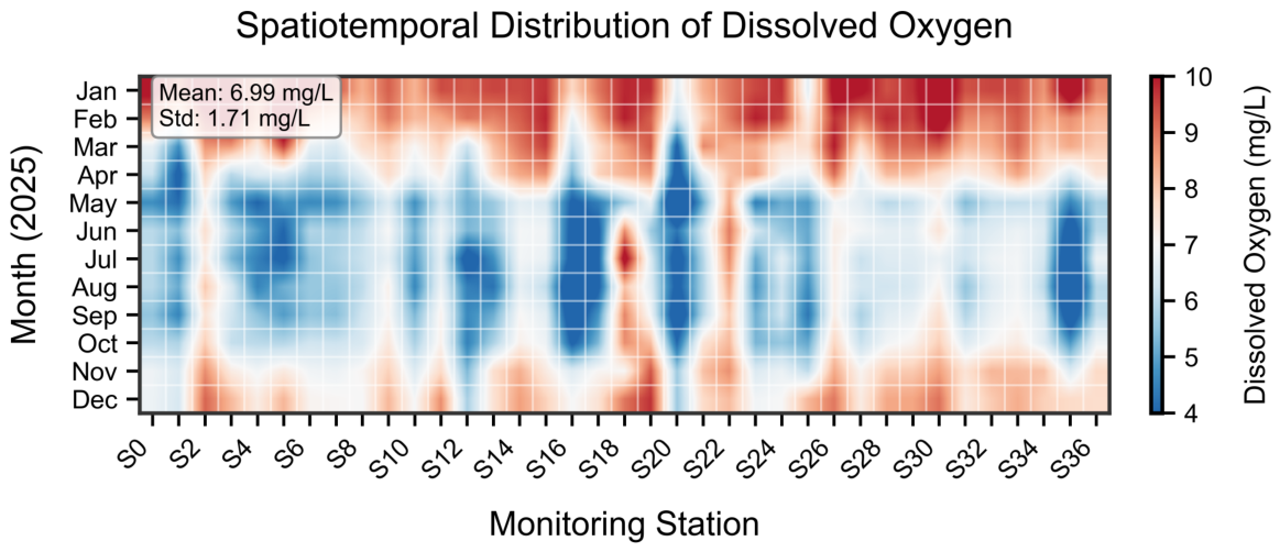
Water quality parameters exhibit significant spatial variability. As shown on the horizontal axis of Figure 2, stations are arranged in numerical order, displaying spatiotemporal variation patterns of dissolved oxygen across all 37 monitoring stations during 2025. From the spatial dimension, dissolved oxygen levels differ markedly across stations. Upstream stations generally exhibit higher concentrations during winter and spring, while midstream and downstream stations show lower values in summer. These differences reflect the combined influences of geographic location, hydrological conditions, and human activities. From the temporal dimension, most stations exhibit seasonal fluctuations with low dissolved oxygen in summer and high in winter, consistent with the temperature-dependent solubility of gases. Seasonal patterns are not perfectly synchronized across stations. Several stations remain in the deep blue low-value zone throughout summer, while a few show red high-value anomalies in specific months, reflecting the impact of extreme weather events or sudden pollution incidents. This spatiotemporal heterogeneity indicates that water quality prediction models must possess the capability to simultaneously adapt to multiple stations and different temporal characteristics.

To evaluate model performance, the dataset is divided chronologically into training, validation, and test sets with a 7:1:2 ratio, yielding 9857, 1408, and 2816 time steps, respectively. The training set is used for model parameter learning, the validation set for hyperparameter tuning and early stopping strategy, and the test set for final performance evaluation. The input sequence length is set to 96 time steps, with prediction horizons of 24, 48, 96, 192, 336, and 720 time steps, corresponding to short-term, medium-term, and long-term prediction tasks, respectively. Training samples are generated via a sliding window strategy, with the sample count ranging from 9041 to 9737 depending on the prediction horizon. Following the widely adopted practice in time series forecasting [18,35,36], we select Mean Squared Error (MSE) and Mean Absolute Error (MAE) as the primary evaluation metrics. MSE assigns a heavier penalty to larger errors, making it suitable for measuring extreme deviations:

$$\begin{array}{c}\mathrm{MSE}={\displaystyle \frac{1}{N}}{\displaystyle \sum _{i=1}^N}{(y_i-{\widehat{y}}_i)}^2\end{array}$$

(25)

MAE, on the other hand, is insensitive to outliers and provides a more stable measure of the average prediction error:

$$\begin{array}{c}\mathrm{MAE}={\displaystyle \frac{1}{N}}{\displaystyle \sum _{i=1}^N}|y_i-{\widehat{y}}_i|\end{array}$$

(26)

To further assess model performance from multiple perspectives, we additionally adopt Root Mean Squared Error (RMSE), Residual Standard Error (RSE), and the General Performance Index (GPI) as supplementary metrics. RMSE shares the same origin as MSE but is scale-aligned with the target variable, while RSE measures the dispersion of prediction residuals, reflecting the stability of the model:

$$\begin{array}{c}\mathrm{RMSE}=\sqrt{\mathrm{MSE}}\end{array}$$

(27)

$$\begin{array}{c}\mathrm{RSE}=\sqrt{{\displaystyle \frac{1}{N-p-1}}{\displaystyle \sum _{i=1}^N}{(y_i-{\widehat{y}}_i)}^2}\end{array}$$

(28)

where p denotes the number of model parameters.

For the General Performance Index (GPI), we follow the formulation of Maroufi and Mehdinejadiani [38], which combines several component metrics as follows:

$$\begin{array}{c}\mathrm{MBE}={\displaystyle \frac{1}{N}}{\displaystyle \sum _{i=1}^N}(y_i-{\widehat{y}}_i)\end{array}$$

(29)

$$\begin{array}{c}\mathrm{TS}=\sqrt{{\displaystyle \frac{(N-1)\times {\mathrm{MBE}}^2}{{\mathrm{RMSE}}^2-{\mathrm{MBE}}^2}}}\end{array}$$

(30)

$$\begin{array}{c}{U}_{95}=1.96\times \sqrt{{\mathrm{RSE}}^2+{\mathrm{RMSE}}^2}\end{array}$$

(31)

$$\begin{array}{c}\mathrm{GPI}=\mathrm{MBE}\times \mathrm{RMSE}\times \mathrm{TS}\times U_{95}\times (1-R^2)\end{array}$$

(32)

For a perfect model, MBE = 0, RMSE = 0, TS = 0, $U_{95}=0$, and $R^2=1$, yielding GPI = 0. Therefore, a GPI value closer to zero indicates better overall prediction performance.

5. Results and Discussion

This chapter comprehensively evaluates and analyzes the performance of HarmonicFormer in water quality time series prediction tasks. First, the experimental setup is introduced, including dataset configuration, evaluation metrics, and comparison models. Subsequently, detailed analysis is conducted across multiple dimensions including overall performance, performance across different prediction horizons, training convergence, ablation experiments, and computational efficiency, validating HarmonicFormer’s advantages in prediction accuracy and computational efficiency. Finally, the sources of model effectiveness, applicable scenarios, and limitations are discussed, providing reference for future research.

5.1. Experimental Setup

The water quality time series dataset used in experiments contains observations of nine water quality parameters at 37 monitoring stations. The prediction task adopts a multi-site mode, utilizing historical data from all 37 stations to simultaneously predict future values at all stations, fully exploiting spatiotemporal correlation information among sites. Independent models are trained separately for each water quality parameter, with all models sharing identical network architecture and hyperparameters. Input data are standardized using Reversible Instance Normalization (RevIN), with normalization parameters fitted only on the training set to avoid test set information leakage.

To validate the effectiveness of HarmonicFormer, it is compared against eight representative baseline models, including temporal Transformer models (TimesNet [28], Autoformer [18]), linear models (DLinear [36]), periodic modeling methods (FreqCycle [34], PhaseFormer [35]), and spatiotemporal graph neural networks (GWN [39], ASTGCN [40], STGCN [23]). Key hyperparameter configurations of HarmonicFormer are as follows: harmonic period length P = 24 (corresponding to 24-h diurnal cycles), number of phase routing layers N = 2, number of routers M = 16, latent dimension of 64, with RevIN normalization enabled to eliminate non-stationarity. These parameter selections will be validated in detail through ablation experiments in Section 5.3.

For training configuration, batch size is set to 32, the Adam optimizer is employed with an initial learning rate of 0.0001, and the learning rate is dynamically adjusted based on validation set loss to accelerate convergence. Maximum training epochs are set to 10, with an early stopping strategy (patience = 3) that terminates training when validation loss fails to improve for three consecutive epochs, avoiding overfitting. All experiments are conducted on a server equipped with two NVIDIA A100-PCIE-40GB GPUs, using Python 3.12.3, PyTorch 2.5.1 framework, and CUDA 12.4. To ensure reproducibility, all experiments use a fixed random seed of 2021.

5.2. Overall Performance and Stepwise Analysis

This section evaluates the prediction performance of HarmonicFormer from an overall perspective. Experiments cover nine water quality parameters and six prediction horizons (24, 48, 96, 192, 336, 720 steps), totaling 54 experimental configurations. HarmonicFormer is compared against eight baseline models using both MSE and MAE metrics for evaluation. The following analysis examines HarmonicFormer’s effectiveness from three perspectives: performance-efficiency tradeoff, complete experimental results, and prediction curve comparison.

5.2.1. Overall Performance

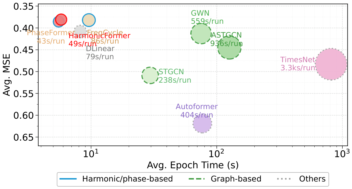
The tradeoff between prediction performance and computational efficiency across different models is compared through the bubble chart in Figure 3. The horizontal axis represents average training time per epoch (logarithmic scale), while the vertical axis represents average MSE. Solid circles denote harmonic or phase modeling methods, dashed circles represent graph neural networks, and dotted circles indicate other Transformer-based models. Ideal models should be located in the upper-left region, corresponding to short training time and low prediction error.

As shown in the figure, HarmonicFormer is located in the optimal upper-left region, achieving the best performance-efficiency balance among periodic modeling methods. Compared to PhaseFormer and FreqCycle, HarmonicFormer achieves lower prediction error while maintaining similar training speed. In contrast, graph neural network models (GWN, ASTGCN, STGCN) exhibit significantly longer training times and markedly higher prediction errors, indicating that spatial dependency modeling based on fixed or globally shared graph structures struggles to capture the nonlocal and time-varying dependencies in water quality data, while also introducing substantial computational burden. Among Transformer-based models, TimesNet has the longest training time with high prediction error, while Autoformer shows unsatisfactory efficiency and performance. The linear model DLinear demonstrates moderate training speed but limited prediction accuracy.

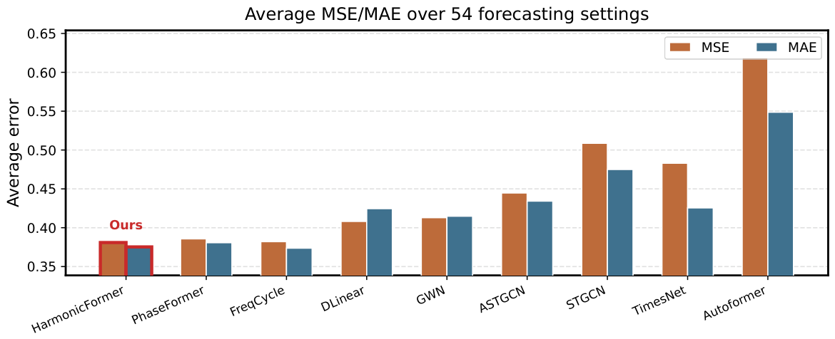
Examining the overall error distribution, Figure 4 presents a holistic view through bar charts of average MSE and MAE across 54 configurations for each model, further validating the aforementioned conclusions. HarmonicFormer achieves an average MSE of 0.38 and average MAE of 0.37, both representing the lowest values. The second-best models are PhaseFormer with MSE of 0.38 and MAE of 0.38, and FreqCycle with MSE of 0.38 and MAE of 0.37, showing small gaps from HarmonicFormer. Spatiotemporal graph models demonstrate relatively weaker overall performance, with STGCN showing average MSE of 0.51 and MAE of 0.47, and ASTGCN showing average MSE of 0.44 and MAE of 0.43, notably higher than periodic modeling methods.

To further quantify performance across parameters and horizons,

Table 2. Cross-variable forecasting results. Each entry reports MSE and MAE. Input length is 96. Best results are in bold, second best are in underline.

Variable	Horizon	HarmonicFormer (Ours)		TimesNet (ICLR 2023) [28]		FreqCycle (AAAI 2026) [34]		PhaseFormer (ICLR 2026) [35]		DLinear (AAAI 2023) [36]		Autoformer (NIPS 2021) [18]		GWN (IJCAI 2019) [39]		ASTGCN (AAAI 2019) [40]		STGCN (IJCAI 2018) [23]
		MSE	MAE	MSE	MAE	MSE	MAE	MSE	MAE	MSE	MAE	MSE	MAE	MSE	MAE	MSE	MAE	MSE	MAE
AN	24	0.2640	0.2743	0.3081	0.3053	0.2788	0.2836	0.2854	0.2962	0.2746	0.3248	0.4190	0.4023	0.2681	0.3128	0.2899	0.3267	0.3230	0.3573
	48	0.3333	0.3186	0.4559	0.3832	0.3458	0.3206	0.3484	0.3315	0.3390	0.3728	0.5132	0.4601	0.3283	0.3576	0.3525	0.3755	0.4492	0.4175
	96	0.4401	0.3740	0.6007	0.4446	0.4524	0.3713	0.4494	0.3802	0.4338	0.4348	0.6778	0.5400	0.4168	0.4171	0.4432	0.4372	0.5905	0.4904
	192	0.5940	0.4451	0.7671	0.5094	0.6059	0.4393	0.5971	0.4472	0.5489	0.5041	0.7408	0.5392	0.5351	0.4906	0.5534	0.5032	0.6210	0.5461
	336	0.7348	0.5082	0.9247	0.5722	0.7551	0.5042	0.7363	0.5088	0.6435	0.5626	0.8867	0.5912	0.6316	0.5519	0.6357	0.5387	0.6859	0.5756
	720	0.8235	0.5520	1.0301	0.6241	0.8513	0.5524	0.8229	0.5508	0.7536	0.6350	1.0667	0.6922	0.7331	0.6260	0.7655	0.6442	0.8188	0.6561
N	24	0.2044	0.2607	0.2459	0.3009	0.2109	0.2702	0.2156	0.2762	0.2183	0.2937	0.3896	0.4497	0.2109	0.2768	0.2370	0.2998	0.3023	0.3328
	48	0.2360	0.2919	0.3279	0.3607	0.2408	0.2985	0.2452	0.3037	0.2566	0.3290	0.3866	0.4385	0.2556	0.3171	0.2895	0.3441	0.3937	0.4006
	96	0.2793	0.3308	0.3951	0.4058	0.2815	0.3336	0.2864	0.3384	0.3158	0.3796	0.4915	0.5084	0.3338	0.3770	0.3529	0.3927	0.5005	0.4601
	192	0.3426	0.3806	0.4490	0.4436	0.3410	0.3791	0.3471	0.3847	0.4090	0.4472	0.4008	0.4376	0.4630	0.4525	0.5495	0.4836	0.6039	0.5298
	336	0.4138	0.4272	0.5525	0.4998	0.4096	0.4233	0.4167	0.4293	0.5183	0.5128	0.4760	0.4858	0.6143	0.5297	0.7257	0.5578	0.7069	0.5879
	720	0.5419	0.4946	0.7216	0.5774	0.5390	0.4925	0.5383	0.4932	0.7709	0.6292	0.6954	0.6165	0.8592	0.6301	0.9976	0.6802	1.0675	0.7402
DO	24	0.1515	0.2462	0.1931	0.2850	0.1718	0.2669	0.1581	0.2534	0.1724	0.2775	0.2716	0.3813	0.1654	0.2666	0.1662	0.2673	0.1786	0.2820
	48	0.1966	0.2852	0.2799	0.3509	0.2140	0.3023	0.2024	0.2914	0.2138	0.3131	0.4179	0.4873	0.2058	0.3046	0.2112	0.3101	0.2318	0.3352
	96	0.2727	0.3433	0.3872	0.4173	0.2864	0.3553	0.2789	0.3486	0.2870	0.3712	0.4444	0.4973	0.2708	0.3569	0.2956	0.3802	0.3132	0.3992
	192	0.3853	0.4172	0.4642	0.4654	0.3959	0.4252	0.3893	0.4202	0.3896	0.4470	0.5733	0.5755	0.3657	0.4261	0.4027	0.4495	0.4377	0.4854
	336	0.5119	0.4927	0.6010	0.5347	0.5166	0.4960	0.5181	0.4963	0.5142	0.5323	0.7467	0.6628	0.5114	0.5267	0.5229	0.5246	0.6066	0.5912
	720	0.7445	0.6277	0.7681	0.6149	0.7253	0.6192	0.7541	0.6316	0.8598	0.7179	1.2201	0.8596	0.9154	0.7340	0.9958	0.7742	0.7975	0.6926
Perm	24	0.2527	0.2944	0.2956	0.3324	0.2640	0.3052	0.2694	0.3065	0.2700	0.3295	0.3920	0.4224	0.2767	0.3154	0.3086	0.3284	0.3432	0.3377
	48	0.3043	0.3286	0.4170	0.4035	0.3120	0.3348	0.3172	0.3383	0.3201	0.3664	0.5733	0.5304	0.3349	0.3586	0.3692	0.3677	0.3970	0.3775
	96	0.3701	0.3697	0.4934	0.4437	0.3730	0.3713	0.3815	0.3763	0.3876	0.4140	0.6357	0.5643	0.4117	0.4017	0.4408	0.4134	0.5128	0.4476
	192	0.4612	0.4228	0.5526	0.4720	0.4568	0.4192	0.4652	0.4255	0.4756	0.4715	0.6062	0.5308	0.4975	0.4470	0.5434	0.4766	0.5788	0.5017
	336	0.5435	0.4661	0.6560	0.5219	0.5318	0.4602	0.5440	0.4671	0.5513	0.5178	0.6578	0.5677	0.5520	0.4864	0.5979	0.5165	0.6773	0.5650
	720	0.7626	0.5631	0.8378	0.6055	0.7527	0.5585	0.7680	0.5656	0.7107	0.6041	0.9288	0.7089	0.6719	0.5777	0.6995	0.5925	0.7574	0.6381
P	24	0.1699	0.2454	0.1990	0.2741	0.1724	0.2514	0.1748	0.2552	0.1741	0.2700	0.3907	0.4543	0.1665	0.2523	0.1746	0.2651	0.1769	0.2651
	48	0.1988	0.2738	0.2806	0.3366	0.2024	0.2783	0.2045	0.2817	0.2049	0.3022	0.4451	0.4839	0.1959	0.2855	0.2047	0.2947	0.2106	0.3036
	96	0.2463	0.3127	0.3250	0.3711	0.2492	0.3149	0.2527	0.3198	0.2529	0.3472	0.4918	0.5192	0.2450	0.3376	0.2605	0.3565	0.2614	0.3529
	192	0.3144	0.3619	0.3841	0.4111	0.3146	0.3609	0.3180	0.3649	0.3165	0.4021	0.6006	0.5754	0.3074	0.3888	0.3348	0.4210	0.3636	0.4394
	336	0.3630	0.3975	0.4342	0.4422	0.3597	0.3931	0.3639	0.3974	0.3694	0.4483	0.4940	0.5218	0.3482	0.4212	0.3879	0.4628	0.4085	0.4754
	720	0.4345	0.4510	0.5521	0.5171	0.4293	0.4454	0.4351	0.4511	0.4810	0.5339	0.7440	0.6821	0.4588	0.5173	0.5646	0.5902	0.5360	0.5795
pH	24	0.2338	0.2816	0.3003	0.3327	0.2616	0.3054	0.2431	0.2930	0.2590	0.3253	0.4467	0.4742	0.2608	0.3113	0.2785	0.3271	0.3529	0.3670
	48	0.2938	0.3255	0.4304	0.4020	0.3160	0.3438	0.3017	0.3355	0.3212	0.3701	0.6359	0.5952	0.3286	0.3566	0.3479	0.3745	0.4603	0.4281
	96	0.3905	0.3873	0.5708	0.4746	0.4090	0.4016	0.3992	0.3942	0.4257	0.4397	0.7712	0.6452	0.4358	0.4226	0.4654	0.4479	0.6305	0.5122
	192	0.5425	0.4696	0.7190	0.5453	0.5569	0.4803	0.5486	0.4741	0.5799	0.5277	0.7897	0.6240	0.5959	0.5075	0.6178	0.5264	0.8053	0.5902
	336	0.7001	0.5440	0.9106	0.6281	0.7168	0.5532	0.7037	0.5464	0.7574	0.6163	0.8332	0.6552	0.7925	0.6043	0.8366	0.6232	0.9766	0.6636
	720	0.9320	0.6466	1.2254	0.7432	0.9617	0.6580	0.9400	0.6501	1.1430	0.7694	1.2593	0.8364	1.4464	0.8577	1.4828	0.8767	1.5370	0.9017
Tur	24	0.2836	0.3111	0.3181	0.3363	0.2860	0.3134	0.2921	0.3235	0.2924	0.3424	0.4492	0.4662	0.2783	0.3247	0.2937	0.3494	0.2872	0.3332
	48	0.3271	0.3427	0.4462	0.4113	0.3300	0.3394	0.3411	0.3592	0.3348	0.3764	0.4709	0.4769	0.3199	0.3615	0.3331	0.3788	0.3308	0.3698
	96	0.3799	0.3816	0.5299	0.4572	0.3795	0.3705	0.3811	0.3806	0.3848	0.4196	0.4971	0.4836	0.3648	0.3976	0.4022	0.4529	0.3918	0.4312
	192	0.4297	0.4166	0.5597	0.4769	0.4281	0.4045	0.4282	0.4146	0.4321	0.4655	0.5077	0.4829	0.4077	0.4397	0.4318	0.4677	0.5751	0.5951
	336	0.4525	0.4346	0.5631	0.4941	0.4503	0.4214	0.4506	0.4339	0.4656	0.5028	0.5652	0.5395	0.4376	0.4818	0.4781	0.5249	0.8829	0.7913
	720	0.5239	0.4805	0.6963	0.5671	0.5212	0.4637	0.5249	0.4808	0.5444	0.5711	0.7433	0.6594	0.6194	0.6253	0.6339	0.6351	1.0761	0.9066
Temp	24	0.0268	0.1035	0.0348	0.1213	0.0276	0.1059	0.0275	0.1058	0.0358	0.1285	0.0567	0.1821	0.0265	0.1073	0.0278	0.1098	0.0297	0.1182
	48	0.0402	0.1310	0.0468	0.1430	0.0378	0.1264	0.0404	0.1324	0.0436	0.1418	0.0871	0.2271	0.0367	0.1311	0.0388	0.1322	0.0532	0.1657
	96	0.0613	0.1642	0.0801	0.1890	0.0578	0.1593	0.0670	0.1773	0.0640	0.1756	0.1176	0.2708	0.0546	0.1628	0.0645	0.1775	0.1228	0.2497
	192	0.1098	0.2370	0.0906	0.2025	0.0878	0.2058	0.1129	0.2420	0.0956	0.2239	1.1699	0.6867	0.0840	0.2152	0.0879	0.2096	0.1766	0.3145
	336	0.1901	0.3226	0.1416	0.2452	0.1267	0.2562	0.1951	0.3268	0.1599	0.2997	0.2724	0.3990	0.1419	0.2937	0.1299	0.2661	0.2083	0.3477
	720	0.4059	0.4905	0.3298	0.3676	0.2447	0.3705	0.4022	0.4870	0.5666	0.5823	2.1010	1.3232	0.5338	0.5642	0.6062	0.6068	0.6379	0.6280
Cond	24	0.2385	0.2510	0.2751	0.2790	0.2511	0.2649	0.2354	0.2649	0.2522	0.2833	0.4373	0.4518	0.2500	0.2660	0.2577	0.2774	0.2658	0.2868
	48	0.2697	0.2847	0.3570	0.3338	0.2812	0.2943	0.2673	0.2940	0.2838	0.3111	0.3879	0.4193	0.2779	0.3045	0.2884	0.3131	0.3068	0.3338
	96	0.3149	0.3244	0.4516	0.3882	0.3254	0.3321	0.3169	0.3307	0.3322	0.3542	0.5314	0.5149	0.3217	0.3477	0.3449	0.3678	0.3666	0.3743
	192	0.3990	0.3900	0.5473	0.4524	0.4059	0.3912	0.3993	0.3935	0.4141	0.4194	0.5265	0.5043	0.4106	0.4264	0.4182	0.4320	0.4832	0.4557
	336	0.4792	0.4494	0.6565	0.5183	0.4850	0.4489	0.4788	0.4506	0.5093	0.4893	0.7731	0.6575	0.5084	0.4957	0.5189	0.4889	0.6911	0.5938
	720	0.6532	0.5393	0.9041	0.6420	0.6435	0.5411	0.6444	0.5392	0.8158	0.6522	1.2143	0.8659	0.8146	0.6521	0.9566	0.7095	0.9682	0.7242
Avg.		0.3809	0.3753	0.4830	0.4255	0.3821	0.3737	0.3857	0.3808	0.4081	0.4245	0.6189	0.5487	0.4130	0.4148	0.4447	0.4343	0.5087	0.4749
Avg. Rank		2.65	2.96	7.76	7.43	2.70	2.83	4.06	4.37	4.91	6.57	8.76	9.13	3.24	5.11	6.39	7.00	7.59	8.04

presents complete MSE and MAE results for nine water quality parameters at six prediction horizons for each model. From an overall perspective, HarmonicFormer achieves an average MSE of 0.3809 and average MAE of 0.3753, both representing the lowest values among all models. With average MSE rank of 2.65 and average MAE rank of 2.96, it significantly outperforms baseline models including TimesNet, Autoformer, GWN, ASTGCN, and STGCN, only slightly higher than FreqCycle’s average MAE rank of 2.83, demonstrating clear advantages across most configurations. For parameters with strong periodicity, HarmonicFormer’s advantages are more pronounced. Taking dissolved oxygen as an example, in 24-step prediction, HarmonicFormer achieves MSE of 0.1515, superior to PhaseFormer’s 0.1581 and FreqCycle’s 0.1718. For pH parameter in 96-step prediction, HarmonicFormer’s MSE of 0.3905 is significantly lower than TimesNet’s 0.5708 and FreqCycle’s 0.4090. These results fully demonstrate that harmonic encoding effectively captures periodic fluctuation patterns, substantially improving prediction accuracy for periodic parameters.

For parameters with relatively weaker periodicity, HarmonicFormer maintains its leading position. In 24-step prediction for conductivity, HarmonicFormer’s MSE of 0.2385 closely approaches the best-performing PhaseFormer’s 0.2354. In 336-step prediction for turbidity, HarmonicFormer’s MSE of 0.4525 essentially matches the best-performing FreqCycle’s 0.4503. Additionally, for temperature parameters, HarmonicFormer achieves optimal or near-optimal results in short-term predictions at 24 and 48 steps. Overall, HarmonicFormer achieves optimal or near-optimal prediction performance across parameters with varying periodicity strengths, demonstrating clear advantages in both prediction accuracy and computational efficiency, validating the effectiveness of harmonic temporal encoding in multi-scale periodic modeling.

We additionally report RMSE, RSE, and GPI as auxiliary metrics to evaluate model performance from broader perspectives.

Table 3. Average performance summary of auxiliary metrics across all variables and forecasting horizons. Each entry reports the average RMSE, RSE, GPI_abs, and the corresponding average ranks. Best results are in bold, second best are in underline. Detailed results for all configurations are provided in Table A1 and Table A2 in the Appendix A.

Model	Avg. RMSE	Avg. RSE	Avg. GPI_abs	Avg. Rank (RMSE/RSE)	Avg. Rank (GPI)
HarmonicFormer	0.5941	0.6941	59.2621	2.33	3.30
TimesNet	0.6681	0.7762	149.5032	7.19	3.43
FreqCycle	0.5943	0.6901	34.0141	2.96	2.63
PhaseFormer	0.5986	0.6994	70.9110	3.54	3.93
DLinear	0.6126	0.7147	518.9856	4.50	5.89
Autoformer	0.7613	0.9139	7362.4039	8.37	6.72
GWN	0.6134	0.7121	1929.8003	3.07	5.52
ASTGCN	0.6360	0.7383	1076.1853	5.69	6.56
STGCN	0.6827	0.7949	2856.6428	7.35	7.04

reports the average values of these metrics across all variables and forecasting horizons, along with the corresponding average ranks. HarmonicFormer achieves an RMSE of 0.5941, outperforming all baseline models, and its RSE of 0.6941 ranks second best, indicating superior performance in both overall error magnitude and prediction stability. In terms of GPI, FreqCycle attains the lowest average GPI_abs of 34.0141 and the best average GPI rank of 2.63, slightly outperforming HarmonicFormer. Nevertheless, HarmonicFormer maintains a competitive GPI rank of 3.30 and outperforms all other baseline models, further confirming its comprehensive advantage across multiple evaluation dimensions.

To quantify model training efficiency,

Table 4. Training efficiency comparison. Epoch time is averaged over all available variable-horizon runs. Lower values are better for time and rank.

Model	Runs	Avg. Epoch Time (s)	Median Epoch Time (s)	Avg. Epochs	Avg. Train Time (s)	Avg. MSE Rank	Avg. MAE Rank
HarmonicFormer	54	5.78	6.61	8.5	49.0	2.65	2.96
FreqCycle	54	9.61	10.69	9.0	86.3	2.70	2.83
GWN	54	75.07	81.21	7.4	558.9	3.24	5.11
PhaseFormer	54	5.52	5.53	7.7	42.6	4.06	4.37
DLinear	53	8.20	8.33	9.7	79.4	4.91	6.57
ASTGCN	54	126.09	134.69	7.4	936.3	6.39	7.00
TimesNet	54	812.86	256.37	4.0	3266.5	7.76	7.43
STGCN	54	29.53	30.89	8.1	237.9	7.59	8.04
Autoformer	54	76.82	64.38	5.3	404.0	8.76	9.13

compiles average epoch time, average train time, and average epochs for each model across 54 configurations. HarmonicFormer achieves an average epoch time of 5.78 s and average train time of 49.0 s. Although PhaseFormer has shorter average train time (42.6 s), HarmonicFormer demonstrates superior prediction accuracy. Compared to FreqCycle’s average train time of 86.3 s, HarmonicFormer holds advantages in both training speed and prediction accuracy. In contrast, graph neural network models GWN, ASTGCN, and STGCN exhibit average train times of 558.9, 936.3, and 237.9 s, respectively. The Transformer-based models TimesNet and Autoformer reach 3266.5 and 404.0 s, all far exceeding HarmonicFormer. These results indicate that HarmonicFormer achieves favorable balance between prediction accuracy and training efficiency, demonstrating high practical application value.

5.2.2. Performance Across Prediction Horizons

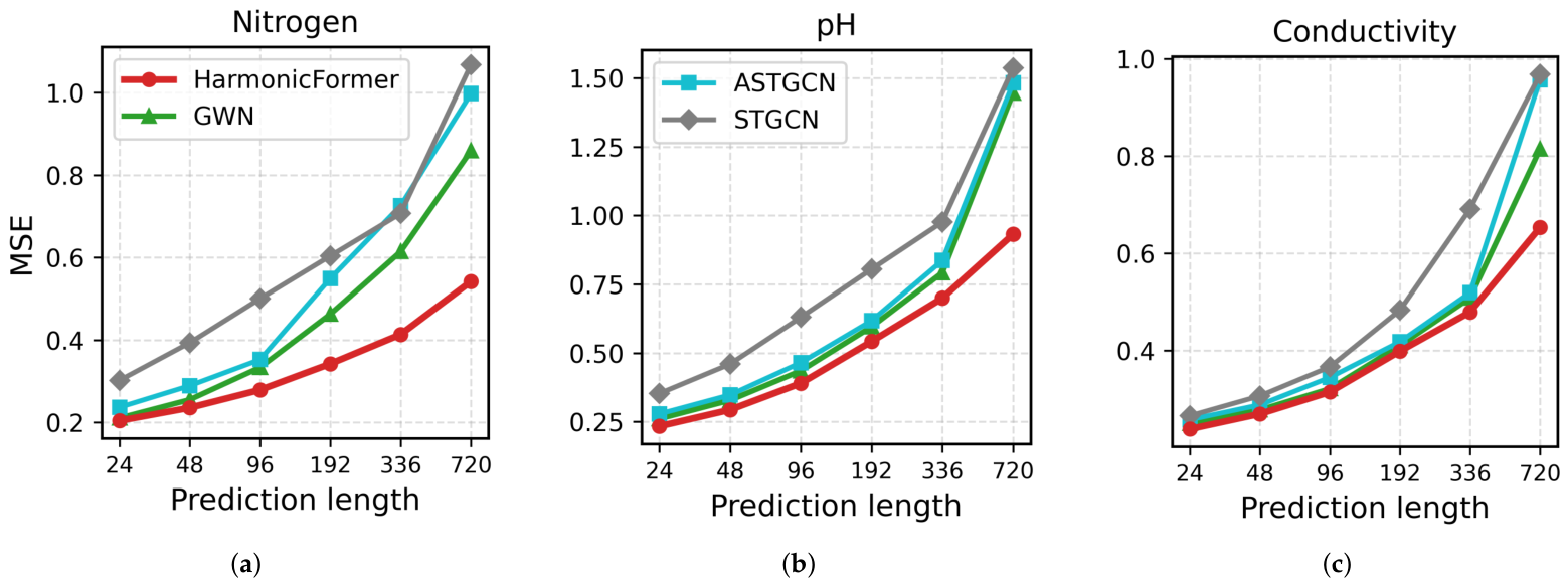
This section further examines how prediction horizon affects model performance. To intuitively illustrate how the performance differences among the models evolve with increasing forecast horizons, Figure 5 compares the MSE values of HarmonicFormer, GWN, ASTGCN, and STGCN for total nitrogen, pH, and conductivity. The MSE of all models increased with the prediction horizon, but the graph-based models exhibited a more pronounced increase. At the 720-step horizon, HarmonicFormer achieved an MSE of approximately 0.54 for total nitrogen, whereas the three graph-based models produced MSE values ranging from 0.86 to 1.07, corresponding to reductions of 36.9–49.2%. For pH and conductivity, HarmonicFormer similarly reduced the MSE by 35.6–39.4% and 19.8–32.5%, respectively. STGCN already exhibited a relatively high error baseline at shorter prediction horizons, whereas the performance gaps between HarmonicFormer and both GWN and ASTGCN widened progressively as the prediction horizon increased. These observations indicate that the differences developed gradually as the prediction range expanded rather than emerging only at the longest horizon.

To verify that the above differences were not attributable to chance, we further examined the late forecast segment, covering steps 193–336 as the prediction progressed from shorter leads toward the 336-step horizon, using experiments with five random seeds. The results are presented in

Table 5. Five-seed forecasting performance and uncertainty over forecast steps 193–336.

Variable	HarmonicFormer	GWN	ASTGCN	STGCN
Total Nitrogen MSE193:336	0.5056	0.7740	0.9978	0.8493
pH MSE193:336	0.8868	1.1484	1.1743	1.0958
Conductivity MSE193:336	0.5901	0.7608	0.8984	0.8990
Three-variable Mean MSE	0.6608	0.8944	1.0235	0.9480
MSE Reduction by HF (%)	–	26.1%	35.4%	30.3%
Mean Lead-wise 95% CI Width	0.0103	0.3336	0.2444	0.3745
CI-width Reduction by HF (%)	–	96.9%	95.8%	97.2%

. In the table, ${\mathrm{MSE}}_{193:336}$ denotes the mean of the exact-lead MSE values over the 144 forecast steps within this interval, obtained from the same directly trained 336-step forecasting model. The MSE reductions were calculated relative to the corresponding graph-based models, while the mean lead-wise 95% confidence interval width was used to characterize training stability across random seeds.

HarmonicFormer achieved a three-variable mean MSE of 0.6608, compared with 0.8944, 1.0235, and 0.9480 for GWN, ASTGCN, and STGCN, respectively, corresponding to reductions of 26.1%, 35.4%, and 30.3%. Its mean lead-wise 95% confidence interval width was only 0.0103, representing a reduction of 95.8–97.2% relative to the three graph-based models. These results indicate that HarmonicFormer maintained both lower prediction errors and greater cross-seed stability in the late forecast segment, where the performance gaps between the models became more pronounced.

To further elucidate the sources of the error differences between HarmonicFormer and GWN, ASTGCN, and STGCN in the late forecast segment, conductivity was selected as a representative variable, and the MSE over forecast steps 193–336 was decomposed into squared bias and residual variance. This decomposition determines whether the observed MSE differences primarily arise from systematic trajectory bias or residual variability. The results are presented in

Table 6. Bias–variance decomposition of conductivity during the late forecast segment (steps 193–336).

Model	Mean MSE193:336	MSE Reduction by HF (%)	$\Delta {\mathbf{Bias}}^2$	$\Delta \mathbf{Var}$	Identified Mechanism
HarmonicFormer	0.5901	–	Reference	Reference	Reference
GWN	0.7608	22.4	>0	<0	Offsetting-bias
ASTGCN	0.8984	34.3	>0	<0	Offsetting-bias
STGCN	0.8990	34.4	Dominant increase	Non-dominant	Bias-dominant

. In the table, $\Delta {\mathrm{Bias}}^2$ and $\Delta \mathrm{Var}$ represent the differences in the corresponding components relative to HarmonicFormer, which serves as the reference model.

The results show that HarmonicFormer achieved the lowest conductivity MSE in this interval, indicating that the sum of its squared bias and residual variance was lower than those of the three graph-based models. Relative to HarmonicFormer, GWN and ASTGCN exhibited increased squared bias but decreased residual variance, indicating that the reduction in residual dispersion was insufficient to offset the increase in bias caused by systematic trajectory deviations. For STGCN, the MSE difference was primarily attributable to squared bias. Overall, the decomposition results indicate that the higher conductivity MSE values of the three graph-based models in the late forecast segment were mainly associated with systematic trajectory bias rather than a simple increase in residual variability.

These observations are consistent with the structural assumptions of the different models. ASTGCN and STGCN rely on fixed spatial topologies to propagate information among monitoring stations. However, water quality parameters may also be influenced by nonlocal and time-varying factors, including hydrological processes, meteorological conditions, and delayed pollutant transport, which may not be adequately represented by a fixed topology. Although GWN can adaptively learn relationships among monitoring stations, the learned structure is globally shared across different samples and forecast steps and lacks a mechanism for dynamic adjustment according to periodic phases. In contrast, HarmonicFormer directly models historical states at corresponding phases through organization according to phase and periodicity and through cross-phase interaction. This reduces its reliance on fixed or globally shared spatial topologies and enables it to preserve long-term forecast trajectories more consistently.

Taken together, the performance and efficiency bubble chart, the complete experimental results, and the prediction curve comparisons show that HarmonicFormer achieved the best average ranking across 54 experimental configurations while maintaining a favorable balance between predictive accuracy and computational efficiency. The bias and variance decomposition further indicated that the higher conductivity MSE of the graph-based models was mainly associated with systematic trajectory bias. Overall, the results suggest that the performance advantage of HarmonicFormer arises from the coordinated effects of organization according to phase and periodicity, cross-phase interaction, and stable temporal modeling, which enable the model to effectively represent periodic variations in water quality parameters and maintain low and stable prediction errors as the forecast horizon increases.

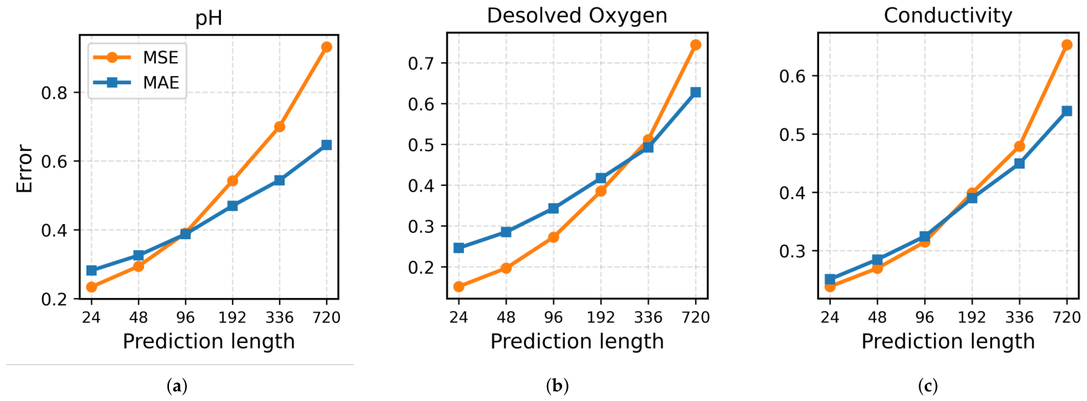
In water quality prediction practice, short-term predictions (24 to 48 steps) primarily serve emergency response and real-time scheduling, while long-term predictions (336 to 720 steps, corresponding to 2 to 4 weeks) support water resource planning and decision-making. Prediction tasks at different time scales impose significantly different requirements on models: short-term prediction relies on near-term trend continuation, whereas long-term prediction requires capturing periodic patterns and suppressing error accumulation. This section reveals model performance characteristics in short-term, medium-term, and long-term predictions by analyzing HarmonicFormer’s performance variations across different prediction horizons. Figure 6 displays the trends of MSE and MAE variation with prediction horizon for HarmonicFormer on three representative water quality parameters.

As shown, prediction errors for all parameters increase monotonically with horizon, but curve shapes and growth rates differ markedly across parameters. Observing the MSE and MAE curves, MSE growth rate generally exceeds that of MAE, indicating that individual large errors have more significant impact on mean squared error in long-term predictions, while mean absolute error exhibits stronger robustness to outliers. For pH parameter, MSE increases from 0.2338 at 24 steps to 0.9320 at 720 steps, with MAE rising from 0.2816 to 0.6466. The curve rises rapidly within the first 96 steps, then continues growing at a slower rate. This pattern reflects that pH values are significantly influenced by diurnal cycles. Harmonic encoding effectively captures short-term fluctuations, but as prediction horizons extend to week-scale timeframes, cumulative errors gradually emerge. For dissolved oxygen parameter, MSE increases from 0.1515 at 24 steps to 0.7445 at 720 steps, with MAE rising from 0.2462 to 0.6277. The curve shows notably slower growth after 336 steps, reflecting harmonic encoding’s effective capture of diurnal fluctuations driven by day-night photosynthesis and respiration. For conductivity parameter, MSE increases from 0.2385 at 24 steps to 0.6532 at 720 steps, with MAE rising from 0.2510 to 0.5393. The curve shape resembles that of dissolved oxygen, with growth slowing after 192 steps. Although conductivity exhibits weaker periodicity, error growth remains stable. Comparing curve shapes across the three parameters horizontally, all exhibit similar two-stage growth patterns: rapid error increase within 96 steps, followed by relatively stable linear growth. This characteristic indicates the model possesses certain stability in long-term prediction, effectively controlling the acceleration of error accumulation.

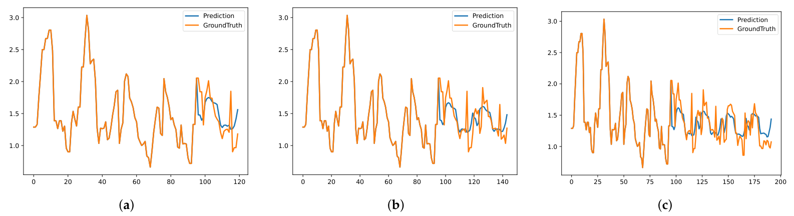
To intuitively demonstrate fitting quality at different prediction horizons, Figure 7 compares the alignment between model outputs and true values at 24-step, 48-step, and 96-step predictions. The x-axis represents the time step index, while the y-axis represents the normalized water quality parameter values after RevIN normalization. As shown, in 24-step short-term prediction, the model prediction curve closely overlaps with true values, accurately tracking short-term fluctuations. In 48-step medium-term prediction, the prediction curve still maintains good synchronization with true values. Although slight local deviations exist, the overall trend and fluctuation patterns remain consistent. In 96-step long-term prediction, deviation between the prediction curve and true values increases somewhat, but the model still captures major variation trends and periodic characteristics.

Further analyzing model performance across different prediction horizons reveals distinct stage-wise characteristics in performance gaps. In the short-term prediction stage (24 and 48 steps), MSE differences between HarmonicFormer and PhaseFormer or FreqCycle remain within 10%. In the medium-term prediction stage (96 and 192 steps), HarmonicFormer’s advantages begin to emerge, achieving approximately 6% and 24% reductions compared to PhaseFormer and Autoformer respectively for pH parameter. In the long-term prediction stage (336 and 720 steps), performance gaps further widen. Notably, spatiotemporal graph neural network models exhibit error divergence after 336 steps, indicating that spatial dependency modeling struggles to ensure long-term prediction stability when lacking periodic modeling mechanisms.

Synthesizing the above analysis, HarmonicFormer maintains stable competitiveness in short-term predictions, with advantages progressively expanding in medium-term and long-term predictions. This characteristic stems from harmonic encoding’s effective capture of diurnal cycle patterns, RevIN normalization’s mitigation of distribution shift, and the phase routing mechanism’s enhancement of long-term dependencies.

5.2.3. Training Efficiency and Convergence

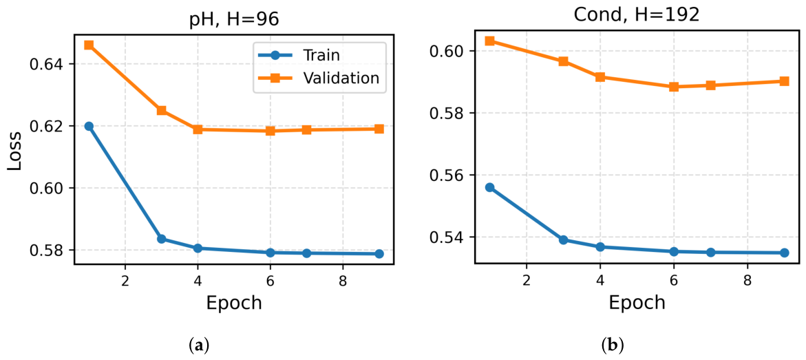
This section validates model efficiency from the training dynamics perspective. Training convergence speed directly impacts time costs for model tuning and deployment. A fast-converging and stable training process serves as an important guarantee for model practicality. Figure 8 displays the training convergence curves of HarmonicFormer on two representative parameters.

As shown, HarmonicFormer exhibits rapid convergence characteristics across different parameters and prediction horizons. In pH parameter training, training loss rapidly decreases from an initial 0.62, stabilizing and converging to 0.58 after epoch 3, while validation loss decreases from 0.65 and stabilizes at 0.62 after epoch 5. In conductivity parameter training, convergence occurs even faster, with training loss converging from 0.56 to 0.53 after epoch 2, and validation loss stabilizing at 0.58 after epoch 3. Training for both parameters completes convergence within 5 epochs. Compared to typical Transformer models requiring dozens or even hundreds of epochs to converge, HarmonicFormer demonstrates significantly higher training efficiency. Observing the gap between training and validation losses, the interval between the two curves consistently remains within 0.05, with validation loss showing no upward trend after convergence, indicating good generalization capability without overfitting. Additionally, both curves exhibit smooth declining trends without severe oscillations or sudden jumps, reflecting training process stability.

Combining training time statistics from Table 4 in Section 5.2.1, HarmonicFormer requires only 5.78 s per epoch on average, with average train time of approximately 49 s, maintaining competitiveness among periodic modeling methods. The model essentially converges within 5 epochs, far lower than graph neural network models ASTGCN at 936 s, STGCN at 238 s, and TimesNet at 3266 s. This efficiency advantage stems from harmonic encoding’s structured periodic modeling approach. Compared to self-attention mechanism’s global dependency computation or graph convolution’s adjacency matrix operations, harmonic encoding reduces model computational complexity through explicit periodic decomposition, while RevIN normalization accelerates gradient propagation, further improving training efficiency. Overall, HarmonicFormer achieves efficient training while ensuring prediction performance, providing a feasible foundation for rapid deployment in practical water quality prediction systems.

5.3. Ablation Study

We examine the effects of harmonic encoding, RevIN normalization, period length, router count, and network depth on prediction performance through multiple ablation experiments. All experiments are conducted under fixed data partitioning and hyperparameters, using MSE and MAE at prediction horizons of 24, 48, and 96 steps as evaluation metrics. First, we analyze the contributions of core modules, with results shown in the Module section of

Table 7. Ablation studies of HarmonicFormer on the water quality forecasting benchmark. Each cell reports MSE and MAE under prediction lengths $L_{\mathrm{out}}\in \{24,48,96\}$. The best result in each block is highlighted in bold, and the second-best result is underlined.

Study	Variant	${\mathit{L}}_{\mathbf{out}}=24$		${\mathit{L}}_{\mathbf{out}}=48$		${\mathit{L}}_{\mathbf{out}}=96$
		MSE	MAE	MSE	MAE	MSE	MAE
Module	HarmonicFormer	0.0578	0.1827	0.0983	0.2387	0.1603	0.3047
	w/o Harmonic Enc.	0.0639	0.1914	0.1035	0.2439	0.1676	0.3121
	w/o RevIN	0.0605	0.1852	0.0982	0.2337	0.1837	0.3282
Period	$P=12$	0.0718	0.2079	0.1085	0.2539	0.1729	0.3194
	$P=24$	0.0578	0.1827	0.0983	0.2387	0.1603	0.3047
	$P=48$	0.0677	0.1975	0.1164	0.2631	0.1679	0.3136
	$P=168$	0.0990	0.2452	0.1187	0.2670	0.1712	0.3189
Routers	$M=4$	0.0586	0.1831	0.0952	0.2320	0.1577	0.3018
	$M=8$	0.0582	0.1826	0.0950	0.2333	0.1617	0.3068
	$M=16$	0.0578	0.1827	0.0983	0.2387	0.1603	0.3047
	$M=32$	0.0600	0.1867	0.0958	0.2342	0.1607	0.3054
Layers	$N=1$	0.0607	0.1878	0.0967	0.2363	0.1611	0.3067
	$N=2$	0.0578	0.1827	0.0983	0.2387	0.1603	0.3047
	$N=3$	0.0604	0.1867	0.0959	0.2339	0.1599	0.3040

. As shown, after removing the harmonic encoding module, MSE for 24-step prediction increases from 0.0578 to 0.0639, representing a 10.6% error increase, indicating that harmonic encoding serves as the model’s core module, with its explicit periodic decomposition effectively capturing diurnal cycle patterns of water quality parameters. After removing RevIN normalization, 24-step prediction error increases by only 4.7%, but 96-step prediction error increases by 14.6%, revealing RevIN’s critical role in mitigating distribution shift for long-term predictions.

Further examination reveals the effects of period length, router count, and network depth. For period length, 24-step prediction MSE with P = 12, 48, and 168 increases by 24.2%, 17.1%, and 71.3% respectively compared to $P=24$. $P=24$ significantly outperforms other settings, consistent with the diurnal cycle characteristics of water quality parameters. For router count, MSE values for $M=4,8$, and 16 are very close, with M = 16 slightly superior. At $M=32$, MSE increases by 3.8%, indicating onset of overfitting. Therefore, $M=16$ achieves optimal balance between capacity and generalization. For network depth, $N=1$ shows 5.0% higher MSE than $N=2$, while $N=3$ demonstrates performance close to $N=2$ but with larger parameter count. Thus, $N=2$ achieves optimal balance between expressiveness and efficiency. Synthesizing the above ablation experiments, harmonic encoding serves as the core module, RevIN is crucial for long-term predictions, and $P=24$, $M=16$, $N=2$ constitute the optimal configuration.

5.4. Discussion

The effectiveness of HarmonicFormer primarily arises from the coordinated use of periodic information modeling and normalization. Harmonic encoding introduces periodic priors, while phase tokenization and cross-phase interaction establish connections between states at corresponding phases across different cycles, enabling the model to preserve cross-cycle information. RevIN further alleviates distribution shifts in nonstationary sequences, thereby improving the stability of long-horizon forecasting.

ASTGCN and STGCN rely on fixed spatial topologies to propagate information among monitoring stations. Such structures are suitable for describing relatively stable local spatial correlations but may not adequately represent the nonlocal and time-varying dependencies induced by hydrological processes, meteorological conditions, and delayed pollutant transport. GWN can adaptively learn relationships among monitoring stations, but the learned graph structure is globally shared across samples and forecast steps and lacks a mechanism for dynamic adjustment according to periodic phases. HarmonicFormer does not require an explicit spatial topology and directly models temporal dependencies through organization according to phase and periodicity. This structural difference is consistent with the systematic trajectory bias observed for the graph-based models in the late forecast segment and provides a plausible explanation for the greater stability of HarmonicFormer over longer forecast horizons.

The current model adopts a fixed period length of $P=24$ and primarily focuses on univariate forecasting. Future research will investigate adaptive period discovery and incorporate external meteorological and hydrological variables to improve the applicability of the model to datasets with different sampling frequencies and to multivariate forecasting tasks.

6. Conclusions

To explicitly model multi-scale periodic features of water quality data and improve long-term prediction performance, this paper proposes the HarmonicFormer model. The model employs a harmonic temporal encoding mechanism that explicitly injects periodic priors such as diurnal cycles through multi-period sinusoidal functions. Combined with phase representation and cross-phase routing layers, it achieves efficient modeling of multi-scale periodicity.

Based on nearly six years of hourly water quality data from 37 monitoring stations in the Pearl River basin, this paper conducts systematic evaluation across nine water quality parameters and six prediction horizons, comparing against eight baseline models. Experimental results demonstrate that HarmonicFormer achieves optimal average MSE and MAE rankings across 54 experimental configurations, with particularly pronounced advantages for parameters with strong periodicity. The model trains efficiently (average 49 s per configuration), with error accumulation effectively controlled in long-term predictions, outperforming compared baseline models. Ablation experiments validate the effectiveness of harmonic encoding, RevIN normalization, and hyperparameter configurations (P = 24, M = 16, N = 2). Through large-scale experiments, this paper validates the superiority of explicit periodic modeling in water quality prediction.

Although HarmonicFormer achieves favorable results, limitations remain including fixed period length and univariate prediction mode. Future work will introduce adaptive period discovery mechanisms, extend to multivariate joint prediction, and incorporate external covariates such as meteorological and hydrological factors to further enhance model generalization capability and practicality.

References

1. Li, L.; Knapp, J.L.A.; Lintern, A.; Ng, G.-H.C.; Perdrial, J.; Sullivan, P.L.; Zhi, W. River water quality shaped by land–river connectivity in a changing climate. Nat. Clim. Change 2024, 14, 225–237. [Google Scholar] [CrossRef] [Scilit]
2. Wu, J.; Cheng, S.-P.; He, L.-Y.; Wang, Y.-C.; Yue, Y.; Zeng, H.; Xu, N. Assessing water quality in the Pearl River for the last decade based on clustering: Characteristic, evolution and policy implications. Water Res. 2023, 244, 120492. [Google Scholar] [CrossRef] [Scilit] [PubMed]
3. Chidiac, S.; El Najjar, P.; Ouaini, N.; El Rayess, Y.; El Azzi, D. A comprehensive review of water quality indices (WQIs): History, models, attempts and perspectives. Rev. Environ. Sci. Bio/Technol. 2023, 22, 349–395. [Google Scholar] [CrossRef] [Scilit] [PubMed]
4. Zhi, W.; Appling, A.P.; Golden, H.E.; Podgorski, J.; Li, L. Deep learning for water quality. Nat. Water 2024, 2, 228–241. [Google Scholar] [CrossRef] [Scilit] [PubMed]
5. Bi, J.; Wang, Z.; Yuan, H.; Wu, X.; Wu, R.; Zhang, J.; Zhou, M.C. Long-term water quality prediction with transformer-based spatial-temporal graph fusion. IEEE Trans. Autom. Sci. Eng. 2025, 22, 11392–11404. [Google Scholar] [CrossRef] [Scilit]
6. Hochreiter, S.; Schmidhuber, J. Long short-term memory. Neural Comput. 1997, 9, 1735–1780. [Google Scholar] [CrossRef] [Scilit] [PubMed]
7. Pyo, J.; Pachepsky, Y.; Kim, S.; Abbas, A.; Kim, M.; Kwon, Y.S.; Ligaray, M.; Cho, K.H. Long short-term memory models of water quality in inland water environments. Water Res. X 2023, 21, 100207. [Google Scholar] [CrossRef] [Scilit] [PubMed]
8. Hu, Z.; Zhang, Y.; Zhao, Y.; Xie, M.; Zhong, J.; Tu, Z.; Liu, J. A water quality prediction method based on the deep LSTM network considering correlation in smart mariculture. Sensors 2019, 19, 1420. [Google Scholar] [CrossRef] [Scilit] [PubMed]
9. Cho, K.; Van Merriënboer, B.; Gulçehre, Ç.; Bahdanau, D.; Bougares, F.; Schwenk, H.; Bengio, Y. Learning phrase representations using RNN encoder–decoder for statistical machine translation. In Proceedings of the 2014 Conference on Empirical Methods in Natural Language Processing (EMNLP); Association for Computational Linguistics: Stroudsburg, PA, USA, 2014; pp. 1724–1734. [Google Scholar]
10. Sutskever, I.; Vinyals, O.; Le, Q.V. Sequence to sequence learning with neural networks. In Proceedings of the Advances in Neural Information Processing Systems; Curran Associates, Inc.: Red Hook, NY, USA, 2014. [Google Scholar]
11. Bai, S.; Kolter, J.Z.; Koltun, V. An empirical evaluation of generic convolutional and recurrent networks for sequence modeling. arXiv 2018, arXiv:1803.01271. [Google Scholar]
12. Wang, Z.; Duan, L.; Shuai, D.; Qiu, T. Research on water environmental indicators prediction method based on EEMD decomposition with CNN-BiLSTM. Sci. Rep. 2024, 14, 1676. [Google Scholar] [CrossRef] [Scilit] [PubMed]
13. Bahdanau, D.; Cho, K.; Bengio, Y. Neural machine translation by jointly learning to align and translate. In Proceedings of the International Conference on Learning Representations (ICLR), San Diego, CA, USA, 7–9 May 2015. [Google Scholar]
14. Chen, H.; Yang, J.; Fu, X.; Zheng, Q.; Song, X.; Fu, Z.; Wang, J.; Liang, Y.; Yin, H.; Liu, Z.; et al. Water quality prediction based on LSTM and attention mechanism: A case study of the Burnett River, Australia. Sustainability 2022, 14, 13231. [Google Scholar] [CrossRef] [Scilit]
15. Rahman, A.; Syeed, M.M.M.; Fatema, K.; Karim, M.R.; Khan, R.H.; Hossain, M.S.; Uddin, M.F. An enhanced multi-head attention-based LSTM model for forecasting the surface water quality index. Water Pract. Technol. 2025, 20, 896–914. [Google Scholar] [CrossRef] [Scilit]
16. Vaswani, A.; Shazeer, N.; Parmar, N.; Uszkoreit, J.; Jones, L.; Gomez, A.N.; Kaiser, Ł.; Polosukhin, I. Attention is all you need. In Proceedings of the Advances in Neural Information Processing Systems; Curran Associates, Inc.: Red Hook, NY, USA, 2017; Volume 30. [Google Scholar]
17. Zhou, H.; Zhang, S.; Peng, J.; Zhang, S.; Li, J.; Xiong, H.; Zhang, W. Informer: Beyond efficient transformer for long sequence time-series forecasting. In Proceedings of the AAAI Conference on Artificial Intelligence; AAAI Press: Washington, DC, USA, 2021; Volume 35, pp. 11106–11115. [Google Scholar]
18. Wu, H.; Xu, J.; Wang, J.; Long, M. Autoformer: Decomposition transformers with auto-correlation for long-term series forecasting. In Proceedings of the Advances in Neural Information Processing Systems; Curran Associates, Inc.: Red Hook, NY, USA, 2021; Volume 34, pp. 22419–22430. [Google Scholar]
19. Nie, Y.; Nguyen, N.H.; Sinthong, P.; Kalagnanam, J. A time series is worth 64 words: Long-term forecasting with transformers. In Proceedings of the International Conference on Learning Representations (ICLR), Kigali, Rwanda, 1–5 May 2023. [Google Scholar]
20. Liu, Y.; Hu, T.; Zhang, H.; Wu, H.; Wang, S.; Ma, L.; Long, M. iTransformer: Inverted transformers are effective for time series forecasting. In Proceedings of the International Conference on Learning Representations (ICLR), Vienna, Austria, 7–11 May 2024. [Google Scholar]
21. Kipf, T.N.; Welling, M. Semi-supervised classification with graph convolutional networks. In Proceedings of the International Conference on Learning Representations (ICLR), Toulon, France, 24–26 April 2017. [Google Scholar]
22. Veličković, P.; Cucurull, G.; Casanova, A.; Romero, A.; Liò, P.; Bengio, Y. Graph attention networks. In Proceedings of the International Conference on Learning Representations (ICLR), Vancouver, BC, Canada, 30 April–3 May 2018. [Google Scholar]
23. Yu, B.; Yin, H.; Zhu, Z. Spatio-temporal graph convolutional networks: A deep learning framework for traffic forecasting. In Proceedings of the Twenty-Seventh International Joint Conference on Artificial Intelligence (IJCAI); Curran Associates, Inc.: Red Hook, NY, USA, 2018; pp. 3634–3640. [Google Scholar]
24. Zhu, Q.; Shen, Z.; Wu, Z.; Zhang, H.; Yuan, J.; Chen, Y. Temporal-relational graph neural network for nearshore seawater quality parameters multivariate multi-step prediction and correlation modelling. Expert Syst. Appl. 2025, 265, 126020. [Google Scholar] [CrossRef] [Scilit]
25. Yuan, M.; Li, Y.; Zhang, L.; Zhao, W.; Zhang, X.; Li, J. Rapid prediction approach for water quality in plain river networks: A data-driven water quality prediction model based on graph neural networks. Water 2025, 17, 2543. [Google Scholar] [CrossRef] [Scilit]
26. Zhou, T.; Ma, Z.; Wen, Q.; Wang, X.; Sun, L.; Jin, R. FEDformer: Frequency enhanced decomposed transformer for long-term series forecasting. In Proceedings of the International Conference on Machine Learning (ICML); Proceedings of Machine Learning Research: Baltimore, MD, USA, 2022; pp. 27268–27286. [Google Scholar]
27. Liu, S.; Yu, H.; Liao, C.; Li, J.; Lin, W.; Liu, A.X.; Dustdar, S. Pyraformer: Low-complexity pyramidal attention for long-range time series modeling and forecasting. In Proceedings of the International Conference on Learning Representations (ICLR), Virtual, 3–7 May 2021. [Google Scholar]
28. Wu, H.; Hu, T.; Liu, Y.; Zhou, H.; Wang, J.; Long, M. TimesNet: Temporal 2D-variation modeling for general time series analysis. In Proceedings of the International Conference on Learning Representations (ICLR), Kigali, Rwanda, 1–5 May 2023. [Google Scholar]
29. Jitha, P.; Vijaya, M.S. Temporal fusion transformer: A deep learning approach for modeling and forecasting river water quality index. Int. J. Intell. Syst. Appl. Eng. 2023, 11, 277–293. [Google Scholar]
30. Ramya, S.; Srinath, S.; Tuppad, P. Data driven multi-stage transformer based framework for intelligent water quality monitoring. Sci. Rep. 2025, 15, 41680. [Google Scholar] [CrossRef] [Scilit] [PubMed]
31. Graziano, A.P.; Jones, R.C. Diel and seasonal patterns in continuously monitored water quality at fixed sites in two adjacent embayments of the tidal freshwater Potomac River. Water 2017, 9, 624. [Google Scholar] [CrossRef] [Scilit]
32. Deng, L.; Chen, K.; Liu, Z.; Wu, B.; Chen, Z.; He, S. Spatiotemporal variation evaluation of water quality in middle and lower Han River, China. Sci. Rep. 2022, 12, 14125. [Google Scholar] [CrossRef] [Scilit] [PubMed]
33. Ding, X.; Chen, Y.; Zeng, H.; Du, Y. Time series prediction of water quality based on NGO-CNN-GRU model: A case study of Xijiang River, China. Water 2025, 17, 2413. [Google Scholar] [CrossRef] [Scilit]
34. Zhang, B.; Yin, S.; Zhu, H.; He, X. FreqCycle: A Multi-Scale Time-Frequency Analysis Method for Time Series Forecasting. In Proceedings of the AAAI Conference on Artificial Intelligence (AAAI), Singapore, 20–27 January 2026. [Google Scholar]
35. Niu, Y.; Deng, J.; Tong, Y. PhaseFormer: From patches to phases for efficient and effective time series forecasting. In Proceedings of the International Conference on Learning Representations (ICLR), Rio de Janeiro, Brazil, 23–27 April 2026. [Google Scholar]
36. Zeng, A.; Chen, M.; Zhang, L.; Xu, Q. Are transformers effective for time series forecasting? In Proceedings of the AAAI Conference on Artificial Intelligence (AAAI), Washington, DC, USA, 7–14 February 2023. [Google Scholar]
37. Kim, T.; Kim, J.; Tae, Y.; Park, C.; Choi, J.-H.; Choo, J. Reversible Instance Normalization for Accurate Time-Series Forecasting against Distribution Shift. In Proceedings of the International Conference on Learning Representations (ICLR), Virtual, 25–29 April 2022. [Google Scholar]
38. Maroufi, H.; Mehdinejadiani, B. A comparative study on using metaheuristic algorithms for simultaneously estimating parameters of space fractional advection-dispersion equation. J. Hydrol. 2021, 602, 126757. [Google Scholar] [CrossRef] [Scilit]
39. Wu, Z.; Pan, S.; Long, G.; Jiang, J.; Zhang, C. Graph WaveNet for Deep Spatial-Temporal Graph Modeling. In Proceedings of the Twenty-Eighth International Joint Conference on Artificial Intelligence (IJCAI-19), Macao, China, 10–16 August 2019. [Google Scholar]
40. Guo, S.; Lin, Y.; Feng, N.; Song, C.; Wan, H. Attention Based Spatial-Temporal Graph Convolutional Networks for Traffic Flow Forecasting. In Proceedings of the AAAI Conference on Artificial Intelligence (AAAI), Honolulu, HI, USA, 27 January–1 February 2019. [Google Scholar]
Figure 1. Overall architecture of the proposed HarmonicFormer.
Water 18 02005 g001
Figure 2. Spatiotemporal variation of dissolved oxygen in the Pearl River Basin (2025).
Water 18 02005 g002
Figure 3. Performance-efficiency trade-off of different models on water quality forecasting.
Water 18 02005 g003
Figure 4. Average MSE and MAE of different models across all 54 configurations.
Water 18 02005 g004
Figure 5. Comparison of MSE across prediction horizons for three representative parameters: (a) total nitrogen; (b) pH; (c) conductivity. All three subfigures compare HarmonicFormer with GWN, ASTGCN, and STGCN over six prediction horizons (24, 48, 96, 192, 336, and 720 steps).
Water 18 02005 g005
Figure 6. MSE and MAE trends across prediction horizons for three representative parameters: (a) pH; (b) dissolved oxygen; (c) conductivity.
Water 18 02005 g006
Figure 7. Comparison of model predictions and true values at different prediction horizons: (a) 24-step; (b) 48-step; (c) 96-step predictions.
Water 18 02005 g007
Figure 8. Training and validation loss convergence curves for pH (a) and conductivity (b).
Water 18 02005 g008