Bulk Decay Coefficient Assessment for Different Water Temperatures: Ensemble Temperature State Estimation Approach

Abstract

Most water supply systems rely on free chlorine residual to ensure disinfection through the network and at the user’s tap. Temperature increase is known to accelerate the chlorine decay process and is typically associated with water quality deterioration. This is a challenging situation under the current climate change scenario, which is bound to increase average temperatures and the intensity and frequency of extreme-temperature events. Moreover, water temperature varies through the supply network due to seasonal changes and thermal interaction, so it is not straightforward to model chlorine evolution through the network considering temperature effects. Previous works have highlighted the importance of considering the Arrhenius formula when accounting for temperature changes in the bulk chlorine decay coefficient (typically characterized through bottle tests), but these studies have never explicitly considered the uncertainty of the bulk decay coefficient itself. Recent studies have identified that the uncertainty of the bulk decay coefficient may be relevant (>15%) and should be considered when cross-comparing bottle test results (e.g., at different temperatures). The aim of this work is to propose a new method that statistically computes the mean and standard deviation of the key parameters in the Arrhenius formula (the reference bulk decay coefficient $k_{b_0}$ and activation coefficient E/R) from free chlorine residual bottle test results (with replicated measurements over samples from the entrance to the network) at different temperatures. This approach (here called the ensemble temperature state estimation approach) ensures that bottle test measurements at different temperatures are jointly assessed to derive an equation that provides the bulk decay coefficient at any water temperature. Therefore, the new method improves the characterization of the bulk decay component (and its associated uncertainty) and could be crucial for improving the understanding and modeling capabilities of complex chlorine dynamics within supply infrastructure.

1. Introduction

Water supply systems must be designed to provide water with adequate pressure and quality to consumers. Many water utilities rely on disinfectant residuals to ensure water quality at treatment works, through the network and at the user’s tap. Nowadays, free chlorine residual is the most widely adopted disinfectant residual worldwide [1,2]. High chlorine levels are not recommended because they are often related to odor/taste issues and DBP (disinfection by-product) formation [3,4]. The generally established minimum free chlorine residual concentration at the point of delivery is 0.2 mg/L [5].

Temperature is known to affect the chlorine decay rate [6,7,8,9,10,11]. In general, temperature increase accelerates chemical reactions [12]. This also applies to the chlorine decay process that takes place at water supply networks. When the temperature of water increases, free chlorine residual concentrations tend to reduce because of the faster reaction processes, potentially leading to chlorine levels below the recommended minimum and water quality issues at terminal areas [13,14]. This tendency is of particular concern under the current and projected climate change conditions [15]. At present, temperature is not systematically monitored in water supply systems, so it is not easy to quantify the implications of temperature increase on supplied water quality [16,17]. However, previous studies show that there is correlation between water quality complaints and air temperature [18,19]. Also, experimental evidence shows that temperature affects the microbiology and physical mobilization processes within water supply systems [20]. The fact that temperature increase is generally associated with water quality deterioration [17] calls for a detailed analysis of the relationship between temperature and free chlorine residual decay rates in water supply systems.

It is important to highlight that temperature changes as water moves through the water supply network [16,21], so chlorine decay rates are expected to vary through the network (spatial variability) and over time (temporal variability). Water temperature at the treatment plant is determined by the source temperature and treatment/storage characteristics. Once treated water enters the network, its temperature varies depending on the temperature gradient with the ground, the ground properties and the contact time, which is determined by the residence time of water within the system [17]. The ground–water thermal interaction is a complex phenomenon, but it is possible to simulate (or at least approximate) how water temperature evolves through the water supply system [21,22,23,24,25]. Even so, accounting for changing temperatures in a chlorine model is not straightforward. Chlorine decay modeling is typically divided into a bulk and a wall decay component. Bulk decay is determined by water quality characteristics and is not influenced by the pipes within the network, so the bulk decay coefficient ($k_b$) is typically characterized by carrying out bottle tests with water samples from the entrance of the network [26]. Wall decay refers to chlorine interaction with the pipe wall, including the biofilm effect, corrosion products and/or any other particles attached to the surface [27]. Due to its complexity, wall decay is frequently computed in practice as the difference between chlorine measurements at a network position and modeled values assuming a bulk decay model only [28,29]. Some authors have adopted the Arrhenius formula to account for temperature changes in bulk decay $k_b$ [9,10,30]. To the best of the authors’ knowledge, there are no previous publications that explicitly consider the temperature effect on any wall decay model. There is evidence that temperature affects microbial abundance [31]/biofilm growth [32,33] and corrosion [34,35,36], but most chlorine wall decay models are empirical in nature, so it is difficult to include the temperature effect without systematic monitoring and modeling consensus. Therefore, it is paramount to improve characterization of the bulk component (and its relationship with temperature) to understand the complexity of the wall interaction.

This work focuses on improving the characterization of free chlorine residual bulk decay rates for different water temperatures. As mentioned before, previous works have relied on the Arrhenius formula to explain how the bulk decay coefficient varies with water temperature [10,30]. This approach is reasonable because the Arrhenius equation is widely accepted [9,37], but it should consider the measurement error effect on $k_b$ estimation and its relationship with temperature. Cejas et al. [27] have recently highlighted that measurement errors may significantly impact the bulk decay coefficient. These authors propose adopting a state estimation methodology to quantify the mean and standard deviation of $k_b$. Coefficients of variation observed for $k_b$ in water samples from different sources (>15%) suggest that the bulk decay coefficient could seem inconsistent among different temperatures/times due to the uncertainty effect. Therefore, neglecting $k_b$ uncertainty could complicate adjusting the Arrhenius equation and computing the bulk decay coefficient at different water temperatures/network positions for some water samples.

The aim of this paper is to propose a new method that statistically computes the mean and standard deviation of the key parameters in the Arrhenius formula (the reference bulk decay coefficient $k_{b_0}$ and activation coefficient E/R) from bottle test results at different temperatures. This approach (here called the ensemble temperature state estimation approach) ensures that bottle test measurements at different temperatures are jointly assessed through state estimation to provide the most likely values of the parameters involved in the Arrhenius equation ($k_{b_0}$ and E/R). State estimation (SE) is here adopted as the core engine because it is a well-established optimization method to combine model equations and noisy measurements [38,39,40,41]. Moreover, it has recently been used to adjust free chlorine residual bulk decay coefficients from bottle test data tracking the associated uncertainty [27]. The novelty of this work lies in providing a comprehensive method to derive the equation that relates the bulk decay coefficient to different water temperatures. This procedure represents an improvement with respect to the state estimation approach presented by Cejas et al. [27], which analyses each bottle test individually (here referred to as the individual temperature state estimation approach) and so may lead to inconsistent $k_b$ values at different temperatures. The ensemble temperature state estimation approach analyses bottle test measurements at different temperatures jointly to ensure the best possible fit for the Arrhenius formula. The resulting equation provides the bulk decay coefficient (and associated uncertainty) at any temperature. This is crucial to compute the bulk decay contribution at any water temperature (i.e., at any network position). Given the changes in temperature that exist through the network, this method could be key to effectively separating the bulk and the wall decay contribution. Therefore, it could be crucial to further understand and explain/model complex water quality dynamics in supply infrastructure under the current climate change scenario.

2. Materials and Methods

This section presents the general state estimation formulation (Section 2.1), which is the conceptual framework adopted in this work to adjust the bulk decay coefficient from bottle test data either with the individual temperature (Section 2.2) or ensemble temperature (Section 2.3) approach. It must be noted that, in this work, input data for both state estimation approaches are bottle test data for bulk water samples taken at the water treatment plant immediately before chlorination. Each sample is collected at the treatment plant and transported to the laboratory, where samples are chlorinated and bottle tests are conducted at different temperatures in parallel using thermostatic baths to see how free chlorine residual concentrations evolve over time. Free chlorine residual levels are measured (with replications) at each time using KEMIO (by Palintest, UK) according to the bottle test with replicate measurements procedure presented in Cejas et al. [27]. A first-order bulk decay model is here assumed to fit the slow decay of free chlorine residual bottle test data through state estimation with both approaches [27]. The first-order bulk decay model is adopted in this work because it has been widely used in the literature before [8,27,42] and it simplifies notation, but any other model could be assumed by adapting the formulation.

Before presenting the formulations themselves, it is interesting to introduce the Arrhenius equation, which is the motivation for the ensemble temperature SE methodology presented in this work. As explained in the Introduction, it is well known that the bulk decay coefficient $k_b$ [1/h] increases with temperature. According to the Arrhenius formula, the bulk decay coefficient for a bottle test $j=\mathrm{1,2},\dots ,n_T$ at a given temperature $T_j$ (here represented as $k_{b_j}=k_b\left(T_j\right);\forall j=\mathrm{1,2},\dots ,n_T$) varies exponentially as follows [43]:

$$k_{b_j}=k_b\left(T_j\right)=k_{b_0}·e^{{\displaystyle \frac{-E/R\left(T_0-T_j\right)}{\left(273+T_0\right)\left(273+T_j\right)}}};\forall j=\mathrm{1,2},\dots ,n_T$$

(1)

where $k_{b_0}$ [1/h] is the reference bulk decay coefficient at a given temperature $T_0$ [°C], E/R [K] is the activation coefficient (computed as the ratio of the activation energy to the universal gas constant) and $n_T$ is the number of bottle tests that are being considered. Both the reference bulk decay coefficient and the activation coefficient may vary widely depending on the water source characteristics. Bulk decay coefficients for different temperatures may range between 0.001 and 0.74 1/h depending on water temperature [42]. The activation coefficient determines how sensitive the water sample is to temperature changes and may vary in one or two orders of magnitude according to previous studies, e.g., 4660–9560 K [9], 5351–8037 K [43], 5000–20,000 K [10] or 6154–12,104 K [13].

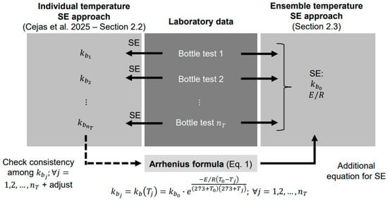
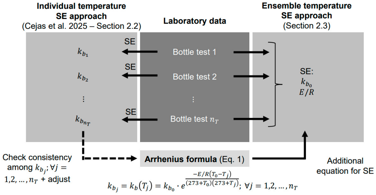
After presenting the SE principles (Section 2.1), Section 2.2 will introduce the individual temperature SE approach presented in Cejas et al. [27], which does not include the Arrhenius equation in the SE formulation. This means that the bulk decay coefficient for each bottle test $k_{b_j};\forall j=\mathrm{1,2},\dots ,n_T$ is computed independently. SE bulk decay coefficients for different temperatures may be compared afterwards through the Arrhenius equation (Equation (1)), but this could lead to potential inconsistencies among temperatures due to the uncertain nature of $k_b$. This was already mentioned in Cejas et al. [27] and will be illustrated with examples in the Results section. The new ensemble temperature SE approach presented in this work (Section 2.3) is conceived to solve this issue. It includes the Arrhenius formula (Equation (1)) as an additional equation in the SE formulation to improve the bottle test–bulk decay model fitting for different temperatures. Figure 1 summarizes the relationship between laboratory data (bottle tests) and each of the approaches, which will be explained in detail in the corresponding sections. Figure 1 shows that for the individual temperature approach, the Arrhenius equation can only be used to contrast results once the individual bulk decay coefficients for each test have been obtained through SE. On the contrary, the Arrhenius equation is an input (together with all bottle test measurements from different temperatures) to obtain the $k_{b_0}$ and E/R parameters of the Arrhenius equation in the ensemble temperature approach. Therefore, the ensemble approach is a more comprehensive methodology to characterize bulk decay dynamics based on bottle tests at different temperatures.

Figure 1. Individual (Cejas et al. [27]–Section 2.2) vs. ensemble temperature (Section 2.3) state estimation approach.

2.1. State Estimation

State estimation (SE) consists of solving an unconstrained weighted least squares optimization problem, which can be generally formulated as [44]:

$$\underset{\mathbf{x}}{\min }{f}_{obj}\left(\mathbf{x}\right)={\displaystyle \frac{1}{2}}{\mathsf{ϵ}\left(\mathbf{x}\right)}^T\mathbf{W}\mathsf{ϵ}\left(\mathbf{x}\right)={\displaystyle \frac{1}{2}}{\left[\mathbf{z}-g\left(\mathbf{x}\right)\right]}^T\mathbf{W}\left[\mathbf{z}-g\left(\mathbf{x}\right)\right]$$

(2)

where $f_{obj}$ represents the objective function, which depends on a vector of state variables $\mathbf{x}\in {\mathbb{R}}^n$. State variables represent the minimum set of independent variables needed to compute the state of the system [41]. Therefore, Equation (2) is conceived to minimize the error or difference between measurements and estimations from state variables, here denoted by vector $\mathsf{ϵ}\left(\mathbf{x}\right)\in {\mathbb{R}}^m$, where $m$ is the number of measurements. The error vector can be written as the difference between the measurement vector $\mathbf{z}\in {\mathbb{R}}^m$ and estimated variables from state variables through the nonlinear relationship $g\left(\mathbf{x}\right):{\mathbb{R}}^n\to {\mathbb{R}}^m$. This difference is here affected by a matrix of measurement weights $\mathbf{W}\in {\mathbb{R}}^{m\times m}$, which is the inverse of the measurement error variance–covariance matrix $\mathbf{W}={\mathbf{C}\mathbf{o}\mathbf{v}}_{\mathbf{z}}^{-1}$. The variance–covariance and weight matrices are usually diagonal because measurements are typically assumed to be independent.

The SE problem described by Equation (2) is typically solved algebraically [40] through the normal equation method:

$${\mathbf{x}}_{(v+1)}={\mathbf{x}}_{\left(v\right)}+{\Delta \mathbf{x}}_{(v+1)}$$

(3)

$${\Delta \mathbf{x}}_{(v+1)}={\left[{\mathbf{J}}_{\left(v\right)}^T{\mathbf{C}\mathbf{o}\mathbf{v}}_{\mathbf{z}}^{-1}{\mathbf{J}}_{\left(\mathit{v}\right)}\right]}^{-1}{\mathbf{J}}_{\left(v\right)}^T{\mathbf{C}\mathbf{o}\mathbf{v}}_{\mathbf{z}}^{-1}\mathsf{ϵ}\left({\mathbf{x}}_{\left(v\right)}\right)$$

(4)

State variables at iteration $v+1$ are computed (Equation (3)) based on the vector of total variation for each state variable at iteration $v+1$ (Equation (4)). The total variation vector considers the derivative of measurements with respect to the state variables through the Jacobian matrix at each iteration ${\mathbf{J}}_{\left(v\right)}\in {\mathbb{R}}^{m\times n}$, which should be full rank. This is something to consider when selecting the set of state variables and deciding the number of measurements ($m$ should always be greater than $n$). This is one of the reasons why replicating measurements in bottle tests is highly encouraged [27]. The iterative process finishes when the norm of the $\Delta \mathbf{x}$ vector falls below a tolerance value ($tol=$ 1 × 10⁻⁶ in this work) or when a maximum of iterations ($N_{max}=$ 100 in this work) is reached. The optimal solution for the state variables is here represented as $\widehat{\mathbf{x}}$, and can be used to infer the variables equivalent to measured values through $g\left(\widehat{\mathbf{x}}\right)$.

One key strength of SE is that it can easily cope with uncertainty propagation. Once the SE optimal solution $\widehat{\mathbf{x}}$ is available, state variable uncertainty can be computed using the First-Order Second-Moment (FOSM) method [44]:

$${\mathbf{C}\mathbf{o}\mathbf{v}}_{\widehat{\mathbf{x}}}={\left[{\mathbf{J}}^T{\mathbf{C}\mathbf{o}\mathbf{v}}_{\mathbf{z}}^{-1}\mathbf{J}\right]}^{-1}$$

(5)

where ${\mathbf{C}\mathbf{o}\mathbf{v}}_{\widehat{\mathbf{x}}}\in {\mathbb{R}}^{n\times n}$ is the variance–covariance matrix of the state variables, which must be computed with the Jacobian matrix at the optimal solution $\widehat{\mathbf{x}}$. The uncertainty of any other set of network variables can be computed by applying the FOSM method again as described in Díaz et al. [44]. The error or difference between measurements and estimated variables at the optimal $\mathsf{ϵ}\left(\widehat{\mathbf{x}}\right)$ can also be used for outlier detection and computation of confidence intervals [27,45]. The details for outlier detection in bottle test fitting will be introduced in the next subsection, after the specific formulation for adjusting the bulk decay coefficient has been presented.

2.2. Individual Temperature State Estimation Approach

Cejas et al. [27] have recently presented an SE methodology to adjust the free chlorine residual bulk decay coefficient in a first-order bulk decay model from bottle test data with measurement replications. In this publication, temperature was constant for all bottle tests, but it was not explicitly included in the SE formulation because it was not the main aim of the study. When the bottle test and SE process is carried out at a specific temperature $T$, the bulk decay coefficient for that temperature is obtained $k_b\left(T\right)$. This means that if the same water sample is subjected to different bottle tests $j=\mathrm{1,2},\dots ,n_T$ (where $n_T$ is the number of bottle tests) at different temperatures $T_j;\forall j=\mathrm{1,2},\dots ,n_T$, different bulk decay coefficients will be obtained for each test $k_{b_j}=k_b\left(T_j\right);\forall j=\mathrm{1,2},\dots ,n_T.$ Since each bulk decay coefficient is obtained independently from the rest, this formulation is here called the “individual temperature state estimation approach”. The formulation presented by Cejas et al. [27] is now introduced explicitly accounting for different bottle test measurements to ease the comparison with the new ensemble approach (see original publication for details on the individual approach).

The formulation of the individual temperature state estimation approach is organized around the free chlorine residual measurement vector ${\mathbf{C}}_{{\mathbf{m}\mathbf{e}\mathbf{a}\mathbf{s}\mathbf{u}\mathbf{r}\mathbf{e}}_{\mathrm{j}}}$ $\in {\mathbb{R}}^{m_{c_j}}$ (where $m_{c_j}$ is the number of chlorine measurements for that bottle test, including measurement replications) and the model parameters needed to estimate free chlorine residual values according to a first-order decay model (slow decay). According to Cejas et al. [27], the chlorine measurement error vector ${\mathbf{E}}_{{\mathbf{m}\mathbf{e}\mathbf{a}\mathbf{s}\mathbf{u}\mathbf{r}\mathbf{e}}_{\mathrm{j}}}$ for each temperature can be written as:

$$\begin{array}{c}{\mathbf{E}}_{{\mathbf{m}\mathbf{e}\mathbf{a}\mathbf{s}\mathbf{u}\mathbf{r}\mathbf{e}}_{\mathrm{j}}}={\mathbf{C}}_{{\mathbf{m}\mathbf{e}\mathbf{a}\mathbf{s}\mathbf{u}\mathbf{r}\mathbf{e}}_{\mathrm{j}}}-\left[C_{{f,model}_j}+\left(C_{{0,model}_j}-C_{{f,model}_j}\right)·e^{-k_{b_j}·{\mathbf{t}}_{\mathrm{j}}}+{\mathbf{E}}_{{\mathbf{m}\mathbf{o}\mathbf{d}\mathbf{e}\mathbf{l}}_{\mathrm{j}}}\right];\\ \forall j=\mathrm{1,2},\dots ,n_T\end{array}$$

(6)

where $C_{{0,model}_j}$ is the initial chlorine concentration for that bottle test, $C_{{f,model}_j}$ is the final chlorine concentration (in case it does not completely decay to 0 mg/L within a reasonable time window), $k_{b_j}$ is the bulk decay coefficient and ${\mathbf{E}}_{{\mathbf{m}\mathbf{o}\mathbf{d}\mathbf{e}\mathbf{l}}_{\mathrm{j}}}\in {\mathbb{R}}^{n_{{times}_j}}$ is the vector of error models for each time, where $n_{{times}_j}$ is the number of average times considered in the bottle test for that specific temperature. The chlorine measurement error vector as provided by Equation (6) represents the difference between free chlorine residual measurement values and free chlorine residual estimated values with the first-order decay model, which follows an exponential decay over time according to vector ${\mathbf{t}}_{\mathrm{j}}\in {\mathbb{R}}^{n_{{times}_j}}$.

Equation (6) is key to adapting the general SE formulation (Equations (2)–(4)) presented in Section 2.1 to the bottle test fitting problem at hand. It involves the first-order bulk decay model, which is the nonlinear function that relates measurements and state variables for each bottle test $g\left({\mathbf{x}}_{\mathrm{j}}\right)$. Cejas et al. [27] assume that all model parameters are state variables. The state variable vector for each bottle test can be written as:

$${\mathbf{x}}_{\mathrm{j}}=\left[C_{{0,model}_j};C_{{f,model}_j};k_{b_j};{\mathbf{E}}_{{\mathbf{m}\mathbf{o}\mathbf{d}\mathbf{e}\mathbf{l}}_{\mathrm{j}}}\right];\forall j=\mathrm{1,2},\dots ,n_T$$

(7)

This implies that the number of state variables is $n_j=3+n_{{times}_j}$ for each test.

Measurements are determined by the number of measurements ($m_{c_j}$) and pseudomeasurements ($m_{p_j}$) for each bottle test $m_j=m_{p_j}+m_{c_j}$. Pseudomeasurements are estimations based on prior knowledge [46]. Cejas et al. [27] recommended adding pseudomeasurements of all state variables in order to enhance redundancy and ensure that the number of measurements is greater than the number of state variables. Note that $m>n$ (or in this case $m_j>n_j;\forall j=\mathrm{1,2},\dots ,n_T$) is a necessary condition for the Jacobian matrix to be full rank. If all state variables are pseudomeasured (i.e., known a priori), the error vector for each bottle test ${\mathsf{ϵ}}_{\mathbf{j}}\left({\mathbf{x}}_{\mathrm{j}}\right)$ can be written as:

$${\mathsf{ϵ}}_{\mathbf{j}}\left({\mathbf{x}}_{\mathrm{j}}\right)=\left[{\mathbf{E}}_{{\mathbf{p}\mathbf{s}\mathbf{e}\mathbf{u}\mathbf{d}\mathbf{o}}_{\mathrm{j}}},{\mathbf{E}}_{{\mathbf{m}\mathbf{e}\mathbf{a}\mathbf{s}\mathbf{u}\mathbf{r}\mathbf{e}}_{\mathrm{j}}}\right]=\left[{\mathbf{z}}_{{\mathbf{p}\mathbf{s}\mathbf{e}\mathbf{u}\mathbf{d}\mathbf{o}}_{\mathrm{j}}}-g\left({\mathbf{x}}_{\mathrm{j}}\right),{\mathbf{E}}_{{\mathbf{m}\mathbf{e}\mathbf{a}\mathbf{s}\mathbf{u}\mathbf{r}\mathbf{e}}_{\mathrm{j}}}\right];\forall j=\mathrm{1,2},\dots ,n_T$$

(8)

where ${\mathbf{z}}_{{\mathbf{p}\mathbf{s}\mathbf{e}\mathbf{u}\mathbf{d}\mathbf{o}}_{\mathrm{j}}}\in {\mathbb{R}}^{m_{p_j}}$ represents the vector of pseudomeasurements. This means that the number of total measurements can also be expressed as the addition of the number of state variables (which are pseudomeasured) and the number of chlorine measurements $m_j=n_j+m_{c_j}$. It should be noted that pseudomeasurements are generally associated with high uncertainty (i.e., high standard deviation) to allow measurements (with lower uncertainty) to condition state estimation results [44]. Default values assumed for state variable pseudomeasurements and free chlorine residual measurements in the individual temperature SE approach are summarized in Table 1 (see Cejas et al. [27] for details). These values are required to build the associated weight matrix (${\mathbf{W}}_{\mathrm{j}}$ in Equation (2)). The associated Jacobian matrix for each bottle test (${\mathbf{J}}_{\mathrm{j}}$ in Equation (4)) can be computed as detailed in the original publication.

Table 1. Default values for state variable pseudomeasurements and free chlorine residual measurements (KEMIO) in the individual temperature state estimation approach (from Cejas et al. [27]).

Type	Variable	Notation	$\mathbf{Mean}\mathit{\mu }$ or Expected Value	$\mathbf{Standard}\mathbf{Deviation}\mathit{\sigma }$
Pseudomeasurement	Initial free chlorine residual concentration according to the model for bottle test $j$ at temperature $T_j$ [mg/L]	$C_{{0,model}_j};$ $\forall j=\mathrm{1,2},\dots ,n_T$	ICC *	0.50
	Final free chlorine residual concentration according to the model for bottle test $j$ at temperature $T_j$ [mg/L]	$C_{{f,model}_j};$ $\forall j=\mathrm{1,2},\dots ,n_T$	0	0.01
	First-order bulk decay coefficient for bottle test $j$ at temperature $T_j$ [1/h]	$k_{b_j};$ $\forall j=\mathrm{1,2},\dots ,n_T$	0.01	0.50
	Error model at each time and for bottle test $j$ at temperature $T_j$ [mg/L]	$E_{{model}_{j_t}};$ $t=\mathrm{1,2},\dots ,n_{times};$ $\forall j=\mathrm{1,2},\dots ,n_T$	0	0.01
Measurement	Free chlorine residual concentration for bottle test $j$ at temperature $T_j$ [mg/L]	$C_{{measure}_j};$ $\forall j=\mathrm{1,2},\dots ,n_T$	Measured in lab	0.065 **

Notes: * ICC = Initial free chlorine residual concentration, as measured in the lab (Cejas et al. [27]). ** According to measurement error characterization tests using KEMIO equipment (Cejas et al. [27]).

Once ${\mathbf{x}}_{\mathrm{j}}$, ${\mathsf{ϵ}}_{\mathbf{j}}\left({\mathbf{x}}_{\mathrm{j}}\right)$, ${\mathbf{W}}_{\mathrm{j}}$ and ${\mathbf{J}}_{\mathrm{j}}$ are defined for all bottle tests ($\forall j=\mathrm{1,2},\dots ,n_T$), the state estimation problem (3)–(4) can be solved for each test at their corresponding temperature $T_j$. As mentioned before, the individual temperature SE formulation (Equations (2)–(8)) does not consider the Arrhenius equation, and this could lead to potential inconsistencies when comparing bulk decay coefficients. SE uncertainty quantification (Equation (5)) and outlier detection are meaningful strategies to identify potential inconsistencies between bottle tests at different temperatures. Outliers may be computed by comparing standardized errors (from the variance–covariance matrix) and confidence intervals. Two possible confidence intervals are computed for free chlorine residual values in this work [27]:

$${CI}_{{\widehat{\mathbf{C}}}_{\mathrm{j}}}={\widehat{\mathbf{C}}}_{\mathrm{j}}\pm {\mathsf{\Phi }}^{-1}\left(1-{\displaystyle \frac{\alpha }{2}}\right)·\sqrt{diag\left({\mathbf{C}\mathbf{o}\mathbf{v}}_{{\widehat{\mathbf{C}}}_{\mathrm{j}}}\right)}$$

(9)

$${TCI}_{{\widehat{\mathbf{C}}}_{\mathrm{j}}}={\widehat{\mathbf{C}}}_{\mathrm{j}}\pm {\mathsf{\Phi }}^{-1}\left(1-{\displaystyle \frac{\alpha }{2}}\right)·\sqrt{diag\left({\mathbf{C}\mathbf{o}\mathbf{v}}_{{\widehat{\mathbf{C}}}_{\mathrm{j}}}\right)+{\sigma }_{C_{measure}}^2}$$

(10)

where ${\widehat{\mathbf{C}}}_{\mathrm{j}}$ represents the expected free chlorine residual values after the SE optimal has been found for each test, and ${\mathbf{C}\mathbf{o}\mathbf{v}}_{{\widehat{\mathbf{C}}}_{\mathrm{j}}}$ is the corresponding variance–covariance matrix. Note that ${CI}_{{\widehat{\mathbf{C}}}_{\mathrm{j}}}$ (Equation (9)) represents the confidence interval of estimated chlorine values for a given confidence interval CI ($\alpha =$ 99% in this work), where ${\mathsf{\Phi }}^{-1}$ represents the inverse of the normal Cumulative Distribution Function (CDF). The total confidence interval ${TCI}_{{\widehat{\mathbf{C}}}_{\mathrm{j}}}$ (Equation (10)) increases ${CI}_{{\widehat{\mathbf{C}}}_{\mathrm{j}}}$ by considering the total variance of free chlorine residual, which includes that associated with SE results (Equation (9)) and measurement variance ${\sigma }_{C_{measure}}^2={0.065}^2{\left(\mathrm{mg}/\mathrm{L}\right)}^2$ (see Table 1).

2.3. Ensemble Temperature State Estimation Approach

The ensemble temperature state estimation approach is the main novelty of this paper. This approach modifies the individual temperature state estimation formulation presented by Cejas et al. [27]—as summarized in Section 2.2—to explicitly include the Arrhenius formula (Equation (1)).

The Arrhenius formula can be introduced through the free chlorine residual measurement error equation (Equation (6) in the individual approach). The bulk decay coefficient for each bottle test $k_{b_j}$ may be substituted in Equation (6) by the Arrhenius formula (Equation (1)), leading to:

$${\mathbf{E}}_{{\mathbf{m}\mathbf{e}\mathbf{a}\mathbf{s}\mathbf{u}\mathbf{r}\mathbf{e}}_{\mathrm{j}}}={\mathbf{C}}_{{\mathbf{m}\mathbf{e}\mathbf{a}\mathbf{s}\mathbf{u}\mathbf{r}\mathbf{e}}_{\mathrm{j}}}-\left\{C_{{f,model}_j}+\left(C_{{0,model}_j}-C_{{f,model}_j}\right)·exp\left[-k_{b_0}·e^{{\displaystyle \frac{-E/R\left(T_0-T_j\right)}{\left(273+T_0\right)\left(273+T_j\right)}}}·{\mathbf{t}}_{\mathrm{j}}\right]+{\mathbf{E}}_{{\mathbf{m}\mathbf{o}\mathbf{d}\mathbf{e}\mathbf{l}}_{\mathrm{j}}}\right\};\forall j=\mathrm{1,2},\dots ,n_T$$

(11)

Note that this equation no longer explicitly involves $k_{b_j}$; it includes the Arrhenius equation parameters $k_{b_0}$ and E/R instead. This means that all free chlorine measurement error vectors for different tests ${\mathbf{E}}_{{\mathbf{m}\mathbf{e}\mathbf{a}\mathbf{s}\mathbf{u}\mathbf{r}\mathbf{e}}_{\mathrm{j}}}\in {\mathbb{R}}^{m_{c_j}};\forall j=\mathrm{1,2},\dots ,n_T$ involve the same $k_{b_0}$ and E/R. In other words, the Arrhenius formula parameters are unknowns that should be computed by jointly assessing all bottle test data.

This means that the set of state variables should include all the bulk decay model parameters in the individual approach (Equation (7)) except for $k_{b_j}$. As a matter of fact, bulk decay first-order model parameters for all bottle tests should be considered state variables together with the Arrhenius equation parameters:

$$\mathbf{x}=\left[\begin{array}{c}{C}_{{0,model}_1};C_{{f,model}_1};{\mathbf{E}}_{{\mathbf{m}\mathbf{o}\mathbf{d}\mathbf{e}\mathbf{l}}_1};C_{{0,model}_2};C_{{f,model}_2};{\mathbf{E}}_{{\mathbf{m}\mathbf{o}\mathbf{d}\mathbf{e}\mathbf{l}}_2};\dots ;\\ C_{{0,model}_{n_T}};C_{{f,model}_{n_T}};{\mathbf{E}}_{{\mathbf{m}\mathbf{o}\mathbf{d}\mathbf{e}\mathbf{l}}_{n_T}};k_{b_0};E/R\end{array}\right]$$

(12)

We must highlight that the state variable vector represented by Equation (12) no longer refers to one set of state variables for each test (like ${\mathbf{x}}_{\mathrm{j}}$ in Equation (7)). In the ensemble temperature SE approach, there is one single state variable vector that comprises state variables from different bottle tests/temperatures. The number of state variables is therefore $n=2\times n_T+{\sum }_{j=1}^{n_T}{n}_{{times}_j}+2$.

In a similar fashion, the error vector of the SE problem must be expressed as:

$$\mathsf{ϵ}\left(\mathbf{x}\right)=\left[{\mathbf{E}}_{{\mathbf{p}\mathbf{s}\mathbf{e}\mathbf{u}\mathbf{d}\mathbf{o}}_1},{\mathbf{E}}_{{\mathbf{p}\mathbf{s}\mathbf{e}\mathbf{u}\mathbf{d}\mathbf{o}}_2},\dots ,{\mathbf{E}}_{{\mathbf{p}\mathbf{s}\mathbf{e}\mathbf{u}\mathbf{d}\mathbf{o}}_{n_T}},{\mathbf{E}}_{{\mathbf{m}\mathbf{e}\mathbf{a}\mathbf{s}\mathbf{u}\mathbf{r}\mathbf{e}}_1},{\mathbf{E}}_{{\mathbf{m}\mathbf{e}\mathbf{a}\mathbf{s}\mathbf{u}\mathbf{r}\mathbf{e}}_2},\dots ,{\mathbf{E}}_{{\mathbf{m}\mathbf{e}\mathbf{a}\mathbf{s}\mathbf{u}\mathbf{r}\mathbf{e}}_{n_T}}\right]=\left[{\mathbf{z}}_{{\mathbf{p}\mathbf{s}\mathbf{e}\mathbf{u}\mathbf{d}\mathbf{o}}_1}-g\left(\mathbf{x}\right),{\mathbf{z}}_{{\mathbf{p}\mathbf{s}\mathbf{e}\mathbf{u}\mathbf{d}\mathbf{o}}_2}-g\left(\mathbf{x}\right),\dots ,{\mathbf{z}}_{{\mathbf{p}\mathbf{s}\mathbf{e}\mathbf{u}\mathbf{d}\mathbf{o}}_{n_T}}-g\left(\mathbf{x}\right),{\mathbf{E}}_{{\mathbf{m}\mathbf{e}\mathbf{a}\mathbf{s}\mathbf{u}\mathbf{r}\mathbf{e}}_1},{\mathbf{E}}_{{\mathbf{m}\mathbf{e}\mathbf{a}\mathbf{s}\mathbf{u}\mathbf{r}\mathbf{e}}_2},\dots ,{\mathbf{E}}_{{\mathbf{m}\mathbf{e}\mathbf{a}\mathbf{s}\mathbf{u}\mathbf{r}\mathbf{e}}_{n_T}}\right]$$

(13)

where ${\mathbf{E}}_{{\mathbf{p}\mathbf{s}\mathbf{e}\mathbf{u}\mathbf{d}\mathbf{o}}_{\mathrm{j}}};\forall j=\mathrm{1,2},\dots ,n_T$ represents the pseudomeasurement error vector and ${\mathbf{z}}_{{\mathbf{p}\mathbf{s}\mathbf{e}\mathbf{u}\mathbf{d}\mathbf{o}}_j}\in {\mathbb{R}}^{m_{p_j}};\forall j=\mathrm{1,2},\dots ,n_T$ is the pseudomeasurement vector for each bottle test. The number of measurements (including pseudomeasurements) is the addition of all measurements and pseudomeasurements for all tests $m={\sum }_{j=1}^{n_T}{m}_{p_j}+{\sum }_{j=1}^{n_T}{m}_{c_j}$. Since all state variables are pseudomeasured, it can also be written as the number of state variables plus the number of free chlorine residual measurements $m=n+{\sum }_{j=1}^{n_T}{m}_{c_j}$. This means that the individual temperature approach solves $n_T$ SE problems of smaller size, but the ensemble temperature approach solves a single SE problem which is much larger. Table 2 summarizes the number of state variables and measurements in the two approaches.

Table 2. Number of state variables/measurements involved in the individual vs. ensemble temperature SE approaches.

Type	Subtype	Individual Temperature SE Approach	Ensemble Temperature SE Approach
State variable	-	$n_j=3+n_{{times}_j};$ $\forall j=\mathrm{1,2},\dots ,n_T$	$n=2\times n_T+{\sum }_{j=1}^{n_T}{n}_{{times}_j}+2$
Measurement	Pseudomeasurement	$m_{p_j}=n_j;$ $\forall j=\mathrm{1,2},\dots ,n_T$	$m_p=n$
	Measurement	$m_{c_j};$ $\forall j=\mathrm{1,2},\dots ,n_T$	$m_c={\sum }_{j=1}^{n_T}{m}_{c_j}$

Regarding the weight matrix $\mathbf{W}$, the ensemble temperature SE approach also assumes greater uncertainty for pseudomeasurement values. Table 3 summarizes the adopted standard deviations for all measurements and pseudomeasurements in this approach. Values are consistent with those included in Table 1 for the individual approach. The mean and standard deviation assumed in Table 1 for the first-order bulk decay coefficient for bottle test $j$ at temperature $T_j$ ($k_{b_j};\forall j=\mathrm{1,2},\dots ,n_T$) is adopted here for the reference bulk decay coefficient at temperature $T_0$ ($k_{b_0}$). Regarding the activation coefficient E/R, it has already been mentioned that it may vary widely depending on the water source. In absence of better information, an average a priori value of 8000 K (in the range of 5000–20,000 provided by Fisher et al. [10]) has been assumed. The adopted standard deviation is also high (2000 K) to reflect the uncertainty of E/R. Since the order of magnitude of the standard deviation of E/R is clearly higher than the rest of the standard deviations assumed for measured/pseudomeasured values, numerical instabilities may arise when computing SE. The numerical conditioning of the matrices involved should be tracked through the process to avoid numerical instabilities.

Table 3. Default values for state variable pseudomeasurements and free chlorine residual measurements (KEMIO) in the ensemble temperature state estimation approach.

Type	Variable	Notation	$\mathbf{Mean}\mathit{\mu }$ or Expected Value	$\mathbf{Standard}\mathbf{Deviation}\mathit{\sigma }$
Pseudomeasurement	Initial free chlorine residual concentration according to the model for bottle test $j$ at temperature $T_j$ [mg/L]	$C_{{0,model}_j};$ $\forall j=\mathrm{1,2},\dots ,n_T$	ICC *	0.50
	Final free chlorine residual concentration according to the model for bottle test $j$ at temperature $T_j$ [mg/L]	$C_{{f,model}_j};$ $\forall j=\mathrm{1,2},\dots ,n_T$	0	0.01
	Error model at each time and for bottle test $j$ at temperature $T_j$ [mg/L]	$E_{{model}_{j_t}};$ $t=\mathrm{1,2},\dots ,n_{times};$ $\forall j=\mathrm{1,2},\dots ,n_T$	0	0.01
	Reference first-order bulk decay coefficient ($T_0$ = 15 °C **) in Arrhenius formula (Equation (1)) [1/h]	$k_{b_0}$	0.01	0.50
	Activation coefficient in Arrhenius formula (Equation (1)) [1/h]	$E/R$	8000	2000
Measurement	Free chlorine residual concentration for bottle test $j$ at temperature $T_j$ [mg/L]	$C_{{measure}_j};$ $\forall j=\mathrm{1,2},\dots ,n_T$	Measured in lab	0.065 ***

Notes: * ICC = Initial free chlorine residual concentration, as measured in the lab (Cejas et al. [27]). ** The reference temperature is assumed to be $T_0$ = 15 °C to avoid coincidences with the temperatures at which bottle tests are carried out in the Results section. *** According to measurement error characterization tests using KEMIO equipment (Cejas et al. [27]).

The Jacobian matrix $\mathbf{J}\in {\mathbb{R}}^{m\times n}$ can be derived by rearranging the chlorine measurement error equation (Equation (11)) so that it expresses free chlorine residual concentrations/measurements (${\mathbf{C}}_{{\mathbf{m}\mathbf{e}\mathbf{a}\mathbf{s}\mathbf{u}\mathbf{r}\mathbf{e}}_{\mathrm{j}}}$) in terms of all the state variables. The Jacobian matrix represents the derivatives of each measurement/pseudomeasurement (in rows) with respect to the assumed state variables (in columns). Since the state variable and error vectors (Equations (12) and (13), respectively) have already been defined for the ensemble approach, and the chlorine measurement error equation (Equation (11)) links all involved terms, the derivatives can be computed as in Cejas et al. [27]. The Jacobian matrix will present a sparse structure in blocks that must be updated through the iteration process.

When the SE problem as described by Equations (2)–(4) finishes, the optimal solution $\widehat{\mathbf{x}}$ will represent the adjusted state variables, including the Arrhenius equation parameters ($k_{b_0}$ and E/R). The mean value of free chlorine residual concentrations at each time can be computed from the first-order bulk decay model equation and uncertainty can be quantified through Equation (5). Uncertainty can also be propagated to the bulk decay coefficient at different temperatures by making use of the derivatives of the Arrhenius equation with respect to $k_{b_0}$ and E/R, and the variance–covariance matrix obtained for those state variables. Since the Arrhenius parameters are known, it is possible to compute the confidence interval and total confidence interval (and detect outliers) as represented by Equations (9) and (10).

It is important to highlight that the ensemble temperature SE formulation is presented in this work in terms of different bottle tests $j=\mathrm{1,2},\dots ,n_T$ and their corresponding temperatures $T_j;\forall j=\mathrm{1,2},\dots ,n_T$. The formulation presented here is compatible with the consideration of bottle tests that each have a different temperature and/or the use of bottle tests that repeat some of the analyzed temperatures. This will be illustrated in the Results section. At least two different temperatures are needed to adjust the Arrhenius equation parameters. If all bottle tests are performed at the same temperature, the individual temperature SE approach (as presented in Cejas et al. [27]) should be applied.

3. Results

The methodology described in Section 2 is here applied to characterize the bulk decay coefficient of three different water sources (A, B, and C) at different temperatures. Water grab samples are collected immediately before chlorination at three treatment works in the region of Castilla-La Mancha (Spain). Each grab sample has a total volume of approximately 20 L and is divided into several subsamples that will be processed at different temperatures following the same laboratory procedure described in Cejas et al. [27]. We will work at different temperatures: 18 or 20 °C (coldest temperature, selected depending on the season, due to the atmospheric temperature changes and isothermal bath availability in the lab), 24 or 26 °C (intermediate temperature, selected depending on the season as well), and 29 °C (hottest temperature). These temperatures are selected in order to cover a wide range of supply temperatures, which may vary between 2 °C and 28 °C at the customer’s tap depending on the country and season [16]. Also, temperatures have been selected to ensure some difference among tests, because temperatures should be effectively different for the Arrhenius equation to be adjusted (about 3–4 °C, although this depends on the water quality characteristics, i.e., the activation coefficient). Also, all bottle tests have been kept below 30 °C to minimize potential instabilities in sodium hypochlorite [47,48] and/or possible deviations in bulk decay estimations [10,15]. Only one refrigerated isothermal bath was available, so the coldest temperature bottle test is carried out once. The intermediate and hottest tests are replicated twice (each) for the sake of understanding the variability of the procedure. Cejas et al. [27] recommended carrying out one bottle test “only” (with replicate measurements) at each temperature, but the two highest-temperature bottle tests will be repeated in parallel in this work for the sake of exploration. Time blocks are slightly displaced among the five tests to ensure that the same person can carry out the quintupled lab test in parallel. Bottle tests will be denoted as “X-E01”, “X-E02”, “X-E02bis”, “X-E03”, and “X-E03bis”, where letter “X” represents the water source (A, B or C); subindices 01, 02 and 03 correspond to the lowest, intermediate and highest temperature conditions (respectively); and suffix “bis” indicates replicate tests performed at the intermediate and high temperatures.

Table 4 includes the main characteristics of the grab samples from each of the three sources/treatment works before starting the bottle tests. TOC is measured once for the total volume of water (20 L), but temperature, pH and ICC are measured for each parallel bottle test (3.8 L) following the procedure described in Cejas et al. [27]. Table 2 shows that TOC is higher for treatment works A (surface water) compared to B and C (groundwater), i.e., they are ordered by decreasing TOC. pH values remain below 9.5 for all water samples, which is the maximum admissible pH for drinking water [49].

Table 4. Grab sample characteristics from sources A, B and C.

Source/Treatment Works	Replication	TOC (mg/L)	Temperature (°C)	ICC (mg/L)	pH (–)
A (surface water)	E01	4.30	20.0	1.08	7.6
	E02		26.0	0.97	7.7
	E02bis		26.0	0.92	7.7
	E03		29.0	1.09	7.7
	E03bis		29.0	1.09	7.8
B (groundwater)	E01	1.70	18.0	0.89	6.6
	E02		24.0	0.96	6.5
	E02bis		24.0	1.02	6.4
	E03		29.0	0.99	6.4
	E03bis		29.0	0.95	6.5
C (groundwater)	E01	0.52	20.0	0.94	6.5
	E02		26.0	1.10	7.2
	E02bis		26.0	0.98	7.4
	E03		29.0	1.16	7.0
	E03bis		29.0	1.05	6.8

Appendix A.1 (Table A1) gathers original data for free chlorine residual measurements over time for the five parallel bottle tests carried out with grab samples from sources A, B and C. Measurements included in Appendix A.1 are now analyzed using the individual temperature SE approach (Section 3.1) and the ensemble temperature SE approach (Section 3.2).

3.1. Individual Temperature State Estimation Approach

This section applies the individual temperature approach presented in Section 2.2 to the five bottle tests carried out with grab samples from water sources A, B and C. The default values presented in Table 1 will be assumed throughout this subsection unless stated otherwise.

3.1.1. Treatment Works A

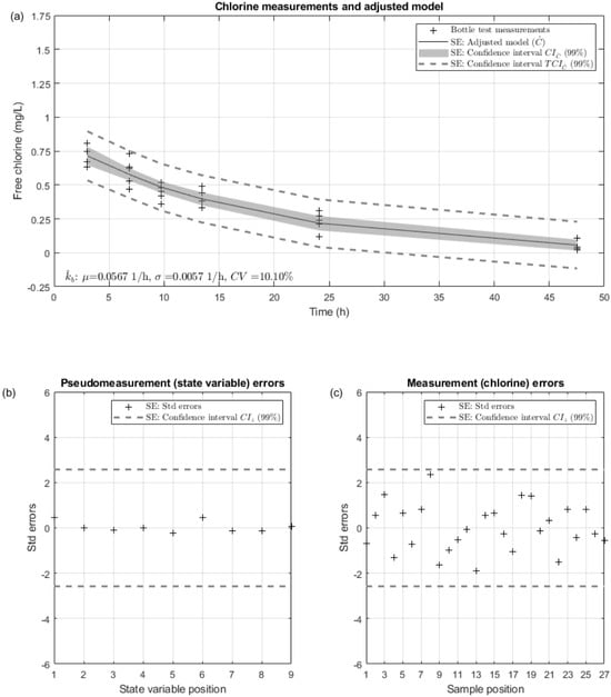
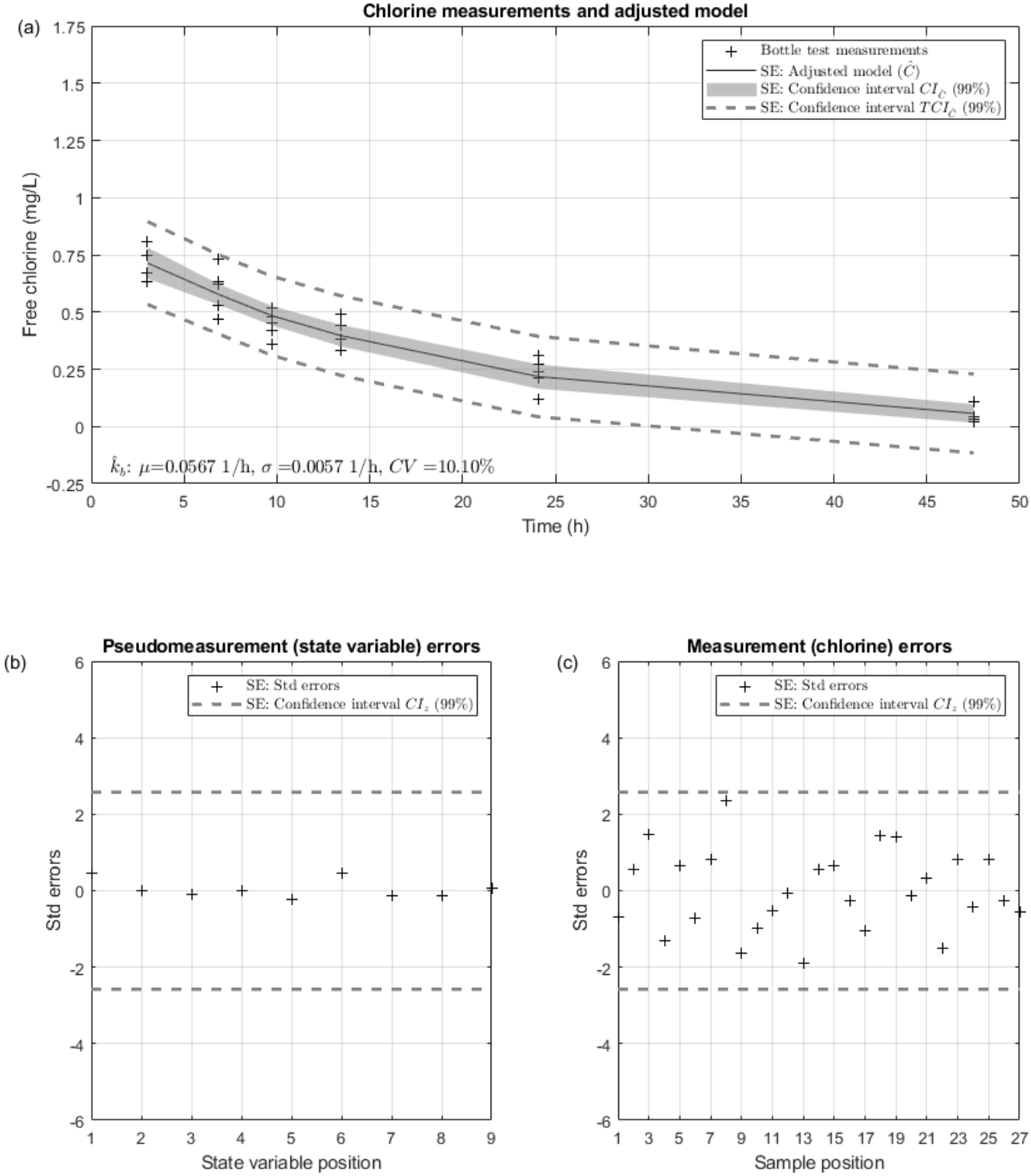
The individual temperature SE approach is applied in this work to each of the five bottle tests carried out with the grab sample from source A (surface water). Figure 2 summarizes the results for the first bottle test at 20 °C (A-E01). Figure 2a shows that the six groups of free chlorine residual measurements (six effective average times, represented with black crosses “+”) progressively reduce their concentration over time, reaching 0 mg/L after approximately 48 h. The adjusted first-order bulk decay model for A-E01 is represented with a black line that passes through bottle test measurements with a well-defined exponential shape, typically associated with high TOC values [27]. This figure also includes the two confidence intervals ${CI}_{\widehat{\mathbf{C}}}$ (Equation (9), represented with a gray shade) and ${TCI}_{\widehat{\mathbf{C}}}$ (Equation (10), represented with dashed gray lines), as well as the mean (0.0567 1/h), standard deviation (0.0057 1/h) and coefficient of variation (10.10%) of the bulk decay coefficient for test A-E01. The coefficient of variation presents an order of magnitude that is consistent with previous results in Cejas et al. [27]. Figure 2b represents the standardized errors for state variable pseudomeasurements. The threshold for outlier detection is in this case $\pm 2.58$ ($\alpha =$ 99% confidence interval), a value that is not reached with A-E01 results. Figure 2c shows the standardized errors for free chlorine residual measurements, which do not exceed the threshold either. This means that there are no outliers for the bottle test at 20 °C. As a matter of fact, there are no outliers for any of the bottle tests carried out with water from source A (highest TOC).

Figure 2. Individual temperature state estimation results for bottle tests A-E01: (a) free chlorine residual measurements and adjusted first-order decay model, (b) standardized pseudomeasurement errors, and (c) standardized measurement errors.

Table 5 summarizes individual temperature SE results for the five bottle tests. This table includes the mean, standard deviation and coefficient of variation for all state variables (Equation (7)) except ${\mathbf{E}}_{{\mathbf{m}\mathbf{o}\mathbf{d}\mathbf{e}\mathbf{l}}_{\mathrm{j}}}$, which was found to be low in general for this type of analysis [27]. According to Table 5, the mean initial free chlorine residual concentrations for the adjusted first-order bulk decay model range between 0.76 mg/L (highest temperature) and 0.85 mg/L (lowest temperature). These values are lower than the originally pseudomeasured values for the initial chlorine concentration or ICC (see Table 1), which range between 0.92 and 1.09 mg/L for source A (see Table 4). This reduction is explained by the high uncertainty of the a priori pseudomeasurement (0.50 mg/L, see Table 1). The uncertainty of the initial chlorine concentrations for the adjusted model (i.e., after SE) is clearly lower than 0.50 mg/L (0.04–0.07 mg/L according to Table 5). Final chlorine concentrations tend to zero (with virtually null standard deviation) because free chlorine residual measurements reach 0 mg/L after roughly 48 h according to Table A1a. Regarding the bulk decay coefficient, in this case mean values tend to increase with temperature (0.0567 1/h for 20 °C, 0.1057–0.1146 1/h for 26 °C and 0.1174–0.1276 1/h for 29 °C) as expected according to the Arrhenius formula (Equation (1)). However, there is some dispersion (which could potentially complicate fitting the Arrhenius formula) at replicated bottle test results for the same temperature. Standard deviations and coefficients of variation also increase slightly with temperature, but again the dispersion associated with replicated tests complicates drawing any final conclusions. It has already been mentioned that the general recommendation is to carry out one single bottle test (with replicated measurements) to characterize the bulk decay coefficient via SE [27]. Nevertheless, this work replicates bottle tests for the intermediate and highest temperature for the sake of exploration, i.e., to identify any potential issues when implementing the proposed methodology. In this work, Cohen’s distance $d$ is used as the metric to compare the goodness of fit/distance between replicated bottle tests at the same temperature [50]. Cohen’s distance is computed here as:

$$d={\displaystyle \frac{\left|{\mu }_1-{\mu }_2\right|}{\sqrt{\frac{{\sigma }_1^2+{\sigma }_2^2}{2}}}}$$

(14)

where ${\mu }_1$ and ${\mu }_2$ represent the mean of the variable that is to be compared (for the two replications) and ${\sigma }_1^2$ and ${\sigma }_2^2$ are the corresponding variances. It is assumed here that Cohen’s distances above 2 suggest that associated normal distributions are likely not the same and values above 3 indicate that normal distributions are clearly different from each other. Table 5 shows that Cohen’s distance for the bulk decay coefficient of replicated bottle tests (for each temperature) is 0.66 at 26 °C and 0.63 at 29 °C, i.e., ${\widehat{k}}_{b_j}$ distributions are consistent. The decision to carry out one or several replications should depend on the cost–benefit relationship for each case. One bottle test for each temperature could be sufficient to understand how the bulk decay coefficient varies with temperature, but it may come with the risk of not having enough evidence for filtering outliers (in this regard, the more replications the better).

Table 5. Individual temperature state estimation results for bottle tests A.

State Variable		T = 20 °C (A-E01)	T = 26 °C (A-E02)	T = 26 °C (A-E02bis)	T = 29 °C (A-E03)	T = 29 °C (A-E03bis)
Initial free chlorine residual concentration ${\widehat{C}}_{{0,model}_j}$	Mean $\mu$ (mg/L)	0.85	0.79	0.83	0.76	0.78
	Std $\sigma$ (mg/L)	0.04	0.06	0.06	0.07	0.07
	CV (%)	5.06	8.17	7.16	9.30	9.44
Final free chlorine residual concentration ${\widehat{C}}_{{f,model}_j}$	Mean $\mu$ (mg/L)	−0.00	0.00	−0.00	0.00	0.00
	Std $\sigma$ (mg/L)	0.01	0.01	0.01	0.01	0.01
	CV (%)	-	-	-	-	-
First-order bulk decay coefficient ${\widehat{k}}_{b_j}$	Mean $\mu$ (1/h)	0.0567	0.1146	0.1057	0.1276	0.1174
	Std $\sigma$ (1/h)	0.0057	0.0142	0.0126	0.0169	0.0157
	CV (%)	10.10	12.36	11.89	13.26	13.36
	Cohen’s $d$ (−)	-	0.66		0.63

3.1.2. Treatment Works B

Table 6 summarizes individual temperature SE results for all five bottle tests derived from grab sample B. As happened with SE results for source A, in this case there is a reasonably good fit to data (nicely defined exponential shape), with only one outlier for measurement 2 in test B-E02, which has been conveniently removed to provide the final values in Table 6. In this case, initial free chlorine residual concentrations are slightly lower than for source A and associated standard deviations and coefficients of variation are lower as well. Regarding the bulk decay coefficient, there is a progressive increase in the mean value with temperature, as happened with source A: 0.0145 1/h for 18 °C, 0.0152–0.0158 1/h for 24 °C and 0.0193–0.0269 1/h for 29 °C. Coefficients of variation change for each test, with values that range between 11.90 and 14.18%. Cohen’s d for the bulk decay coefficient shows that replications at 24 °C provide similar $k_b$ distributions (d = 0.30) but highlights that associated normal distributions are likely not the same at 29 °C (d = 2.53 > 2). This may be explained by the high temperature, as temperatures above 30 °C have been related to instabilities in sodium hypochlorite [47,48] and/or possible deviations in bulk decay estimations [10,15].

Table 6. Individual temperature state estimation results for bottle tests B.

State Variable		T = 18 °C (B-E01)	T = 24 °C (B-E02)	T = 24 °C (B-E02bis)	T = 29 °C (B-E03)	T = 29 °C (B-E03bis)
Initial free chlorine residual concentration ${\widehat{C}}_{{0,model}_j}$	Mean $\mu$ (mg/L)	0.66	0.65	0.75	0.69	0.73
	Std $\sigma$ (mg/L)	0.03	0.03	0.03	0.04	0.03
	CV (%)	4.43	4.93	3.90	5.22	4.39
Final free chlorine residual concentration ${\widehat{C}}_{{f,model}_j}$	Mean $\mu$ (mg/L)	0.00	−0.00	0.00	0.00	−0.00
	Std $\sigma$ (mg/L)	0.01	0.01	0.01	0.01	0.01
	CV (%)	-	-	-	-	-
First-order bulk decay coefficient ${\widehat{k}}_{b_j}$	Mean $\mu$ (1/h)	0.0145	0.0158	0.0152	0.0269	0.0193
	Std $\sigma$ (1/h)	0.0019	0.0022	0.0018	0.0035	0.0024
	CV (%)	13.39	14.18	11.90	13.08	12.35
	Cohen’s $d$ (−)	-	0.30		2.53

3.1.3. Treatment Works C

Table 7 summarizes individual temperature SE results for bottle tests carried out with grab sample C. Again, the adjusted initial chlorine concentration presents a low standard deviation and coefficient of variation. However, there are noticeable differences in the final chlorine concentration. We must highlight that free chlorine residual measurements do not reach 0 mg/L in tests C-E01, C-E02 and C-E02bis (see Table A1c), so the a priori standard deviation of the final chlorine concentration (pseudomeasurement) has been increased here to 0.50 mg/L in these tests as recommended by Cejas et al. [27]. This leads to final free chlorine residual values that differ from zero to obtain a better fit of the chlorine decay asymptote. Even so, there is one outlier for test C-E01 (measurement 16 in Table A1c), which has been removed to provide the final values in Table 7. Also, there is one outlier for test C-E03bis (measurement 19 in Table A1c), which has also been removed to obtain the final values in Table 7. The fact that there are more outliers for this grab sample is partly explained because of the value of the bulk decay coefficient, which is one order of magnitude lower than that obtained for samples A and B. This means that bulk decay tends to be linear (rather than exponential), a behavior that has already been associated with groundwater with low TOC in similar studies [27]. Table 7 shows that the mean bulk decay coefficient does not always increase with temperature depending on the bottle test replication. We obtained 0.0022 1/h for 20 °C, 0.0051–0.0123 1/h for 26 °C and 0.0114–0.0127 for 29 °C. This means that if we had only carried out bottle tests C-E01, C-E02 and C-E03bis, the bulk decay coefficient would not systematically increase (as expected according to the Arrhenius formula). This inconsistency is explained in practice by the uncertainty of the bulk decay coefficient. Note that the associated coefficients of variation range between 9.27 and 50.94%. They are greater for the first three tests due to the increased standard deviation assumed for the final free chlorine residual concentration. Cohen’s ds show that there is a significant difference between tests at 26 °C (d = 3.66) and some level of difference between tests at 29 °C (d = 1.08). These results illustrate that characterizing the bulk decay coefficient uncertainty becomes especially important when dealing with water samples with low TOC. In these scenarios, adjusting the Arrhenius equation is even more troublesome, and should manage uncertainty correctly. This is possible through the ensemble temperature approach presented in the next subsection.

Table 7. Individual temperature state estimation results for bottle tests C.

State Variable		T = 20 °C (C-E01)	T = 26 °C (C-E02)	T = 26 °C (C-E02bis)	T = 29 °C (C-E03)	T = 29 °C (C-E03bis)
Initial free chlorine residual concentration ${\widehat{C}}_{{0,model}_j}$	Mean $\mu$ (mg/L)	0.83	1.00	0.96	0.81	0.92
	Std $\sigma$ (mg/L)	0.02	0.03	0.02	0.03	0.03
	CV (%)	2.47	2.83	2.53	3.37	2.94
Final free chlorine residual concentration ${\widehat{C}}_{{f,model}_j}$	Mean $\mu$ (mg/L)	−0.27	0.29	0.21	0.00	−0.00
	Std $\sigma$ (mg/L)	0.40	0.04	0.12	0.01	0.01
	CV (%)	−144.77	13.61	58.82	-	-
First-order bulk decay coefficient ${\widehat{k}}_{b_j}$	Mean $\mu$ (1/h)	0.0022	0.0123	0.0051	0.0127	0.0114
	Std $\sigma$ (1/h)	0.0011	0.0022	0.0017	0.0013	0.0011
	CV (%)	50.94	17.91	33.91	10.60	9.27
	Cohen’s $d$ (−)	-	3.66		1.08

3.2. Ensemble Temperature State Estimation Approach

This section applies the ensemble temperature approach presented in Section 2.3 to bottle tests for grab samples A, B and C. Section 3.1 has illustrated that replicating bottle tests at the same temperature may lead to bulk decay coefficient distributions that are different. For this reason, rather than running the ensemble approach with three bottle tests/temperatures (which would mean having to choose three out of the five bottle test data available), we will be running the ensemble approach using data from the five bottle tests.

In all cases, it will be assumed that $T_0=15$ °C. This temperature has been selected to avoid coincidences with the temperatures at which bottle tests are carried out in this work. Also, pseudomeasurement/measurement values will be assumed equal to those in Table 3 unless stated otherwise.

3.2.1. Treatment Works A

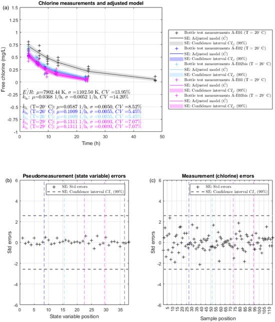
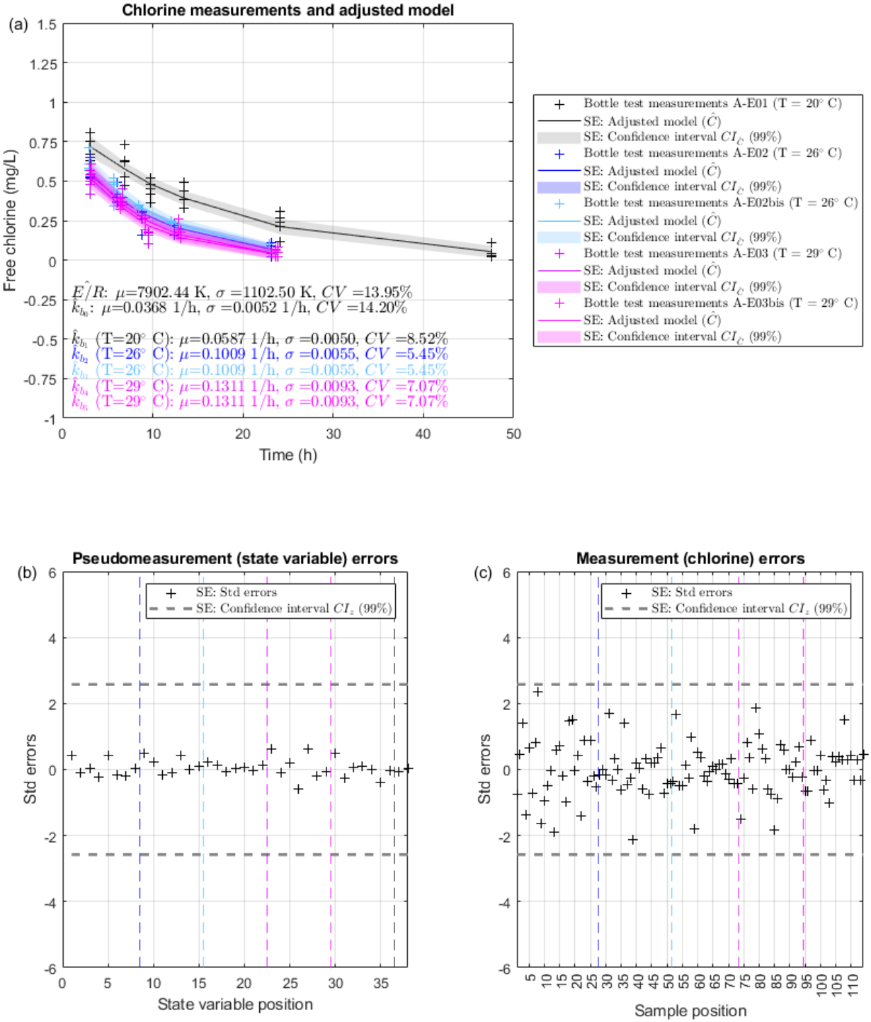
Results for the ensemble temperature SE approach are represented in Figure 3. Figure 3a gathers the bottle test data (crosses ‘+’), adjusted first-order bulk decay model (solid line) and confidence interval ${CI}_{\widehat{\mathbf{C}}}$ (Equation (9), shaded) for all bottle tests (gray for A-E01 at 20 °C, blue and light blue for A-E02 and A-E02bis at 26 °C, purple and pink for A-E03 and A-E03 bis at 29 °C). Only ${CI}_{\widehat{\mathbf{C}}}$ (not ${TCI}_{\widehat{\mathbf{C}}}$) is represented here to ease visualization and comparison across temperatures. Data and adjusted model results for T = 20 °C (in gray) are clearly different than 26 °C (in blues) and 29 °C (in pinks), which present some degree of overlap. This happens because temperatures are fairly close and confidence intervals present a width that is determined by the associated standard deviation. Overall, blue decay (26 °C) appears below gray decay (20 °C) and pink decay (29 °C) happens below blue decay (as it should). Figure 3a also includes the resulting mean (7902.44 K), standard deviation (1102.50 K) and coefficient of variation (13.95%) of the activation coefficient E/R. These values prove that the assumed mean and standard deviation (8000 and 2000 K, respectively) are a good assumption. This idea is reinforced by the fact that there are no outliers in pseudomeasurements/state variables (Figure 3b) nor free chlorine residual measurements (Figure 3c). Note that vertical-colored dashed lines have been introduced to define the limit of state variables and measurements corresponding to each of the five bottle tests. Regarding the reference bulk decay coefficient ($k_{b_0})$, for this combination of bottle test data, the resulting mean is 0.0368 1/h, the associated standard deviation is 0.0052 1/h and the coefficient of variation is 14.20%. This mean reference value (at 15 °C) is lower than the mean bulk decay coefficient for 20 °C in the individual approach (0.0567 1/h) as it should be expected according to the Arrhenius formula. The coefficient of variation obtained with the ensemble approach (14.20%) is similar in order of magnitude to the range of the individual approach (10.10–13.36%) despite the additional uncertainty of the activation coefficient (which is high). The strong point of the ensemble approach is that it guarantees that bulk decay coefficients will be unique for each temperature (estimated ${\widehat{k}}_{b_j}$ values are constant for each temperature—see constant values for blues and pinks) and consistent among temperatures. In other words, it is possible to compute the bulk decay coefficient at any temperature based on the adjusted $k_{b_0}$ and E/R. It should also be noted that the standard deviation and CV obtained for the bulk decay coefficient at different temperatures according to the ensemble approach (after propagation of uncertainty values for $k_{b_0}$ and E/R) is lower (CV ranges 5.45–8.52%) than that of $k_{b_0}$ due to a strong negative cross-correlation (−5.33) between the parameters involved in the Arrhenius equation in the variance–covariance state variable matrix. This implies that even though the uncertainty obtained for $k_{b_0}$ with the ensemble approach does not reduce with respect to the uncertainty obtained for $k_{b_j};\forall j=\mathrm{1,2},\dots ,n_T$ with the individual approach, thanks to the relationship between $k_{b_0}$ and E/R, there is a decrease in the propagated uncertainty for $k_{b_j};\forall j=\mathrm{1,2},\dots ,n_T$ with the ensemble approach.

Figure 3. Ensemble temperature state estimation results for treatment works A: (a) free chlorine residual measurements and adjusted first-order decay model, (b) standardized pseudomeasurement errors, and (c) standardized measurement errors.

3.2.2. Treatment Works B

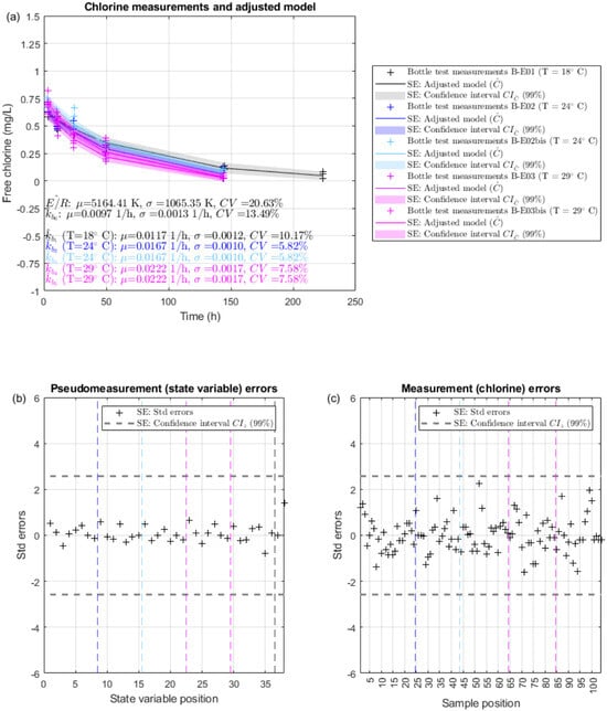
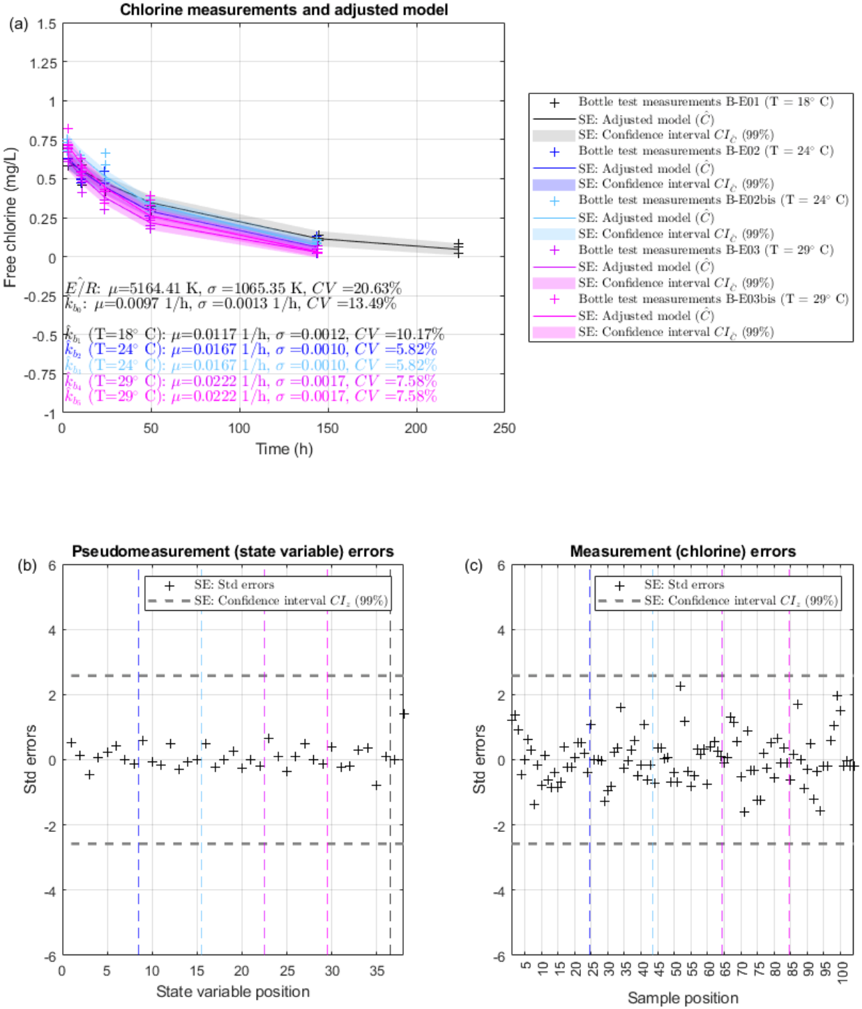
The same methodology is now applied to grab sample B. As explained in Appendix A.2, one outlier (measurement 2 in B-E02) is identified with the ensemble temperature SE approach, just like with the individual analysis. Figure 4 shows ensemble temperature SE approach results once the outlier has been removed. Like in Figure 3, Figure 4a shows that there is some degree of overlap between temperatures, but in general decay data/results for 29 °C (in purple/pink) are lower than those for 24 °C (in blues) and 18 °C (in gray), as should be expected according to the Arrhenius formula. The comparison between Figure A1 (in Appendix A.2) and Figure 4 shows that removing the outlier has little effect on the estimated state variables, as this is only one measurement out of the 105 free chlorine residual measurements available for grab sample B (Table A1b).

Figure 4. Ensemble temperature state estimation results for treatment works B (without outlier): (a) free chlorine residual measurements and adjusted first-order decay model, (b) standardized pseudomeasurement errors, and (c) standardized measurement errors.

According to Figure 4a, the mean (5164.41 K), standard deviation (1065.35 K) and coefficient of variation (20.63%) of the activation coefficient is again consistent with the assumed pseudomeasurements for grab samples B (see Table 3). Regarding the bulk decay coefficient, the mean reference value is 0.0097 1/h in this case, its standard deviation is 0.0013 1/h and the associated coefficient of variation is 13.49%. These values are similar to those obtained for 18 °C in the individual analysis (mean = 0.0145 1/h, std = 0.0019 1/h and CV = 13.39%). Again, there is a reduction in the uncertainty of the bulk decay coefficient for different temperatures when comparing results for the ensemble approach (5.82–10.17%, Figure 4a) and the individual approach (11.90–14.18%, see Table 6).

3.2.3. Treatment Works C

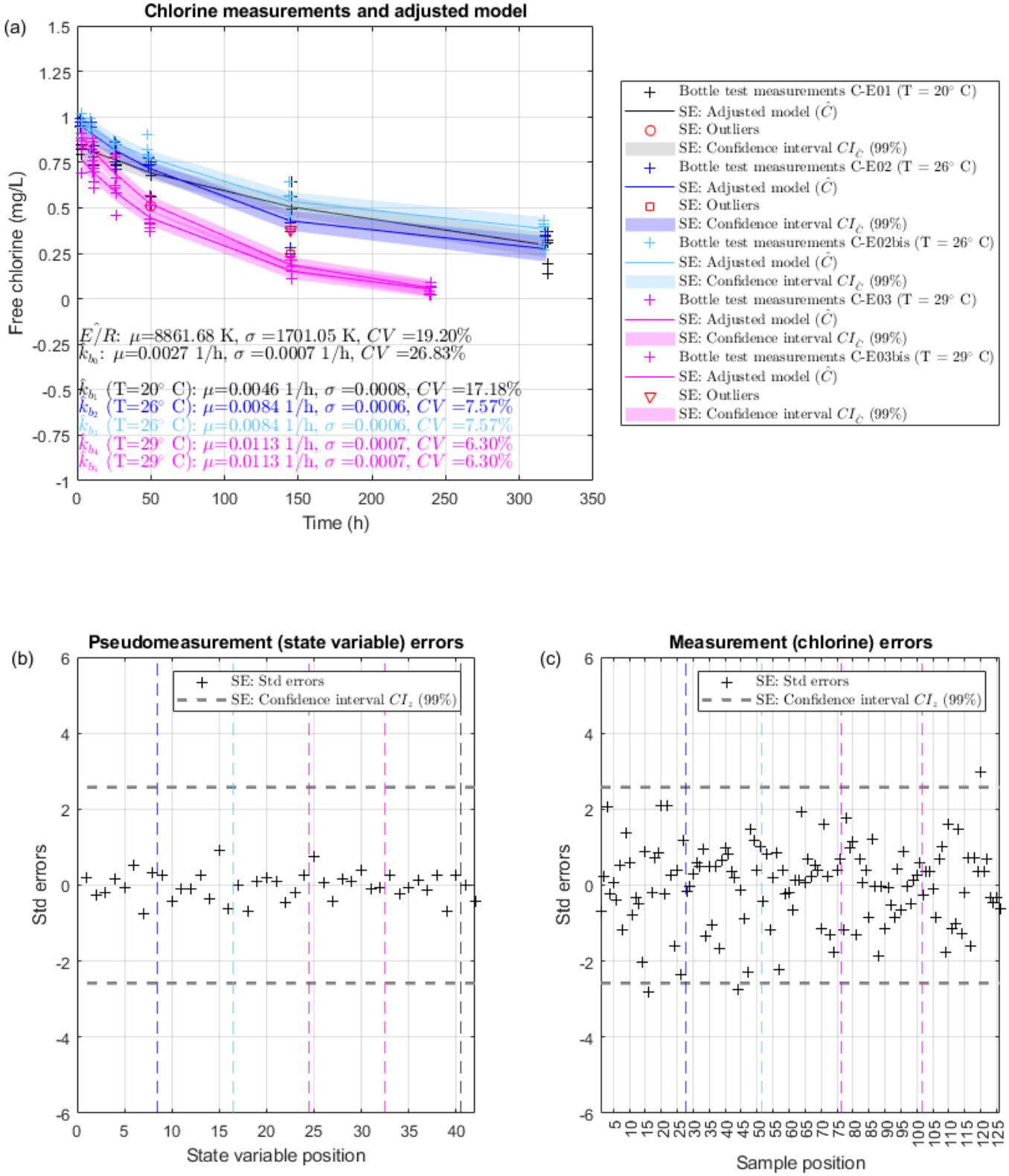
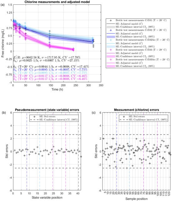
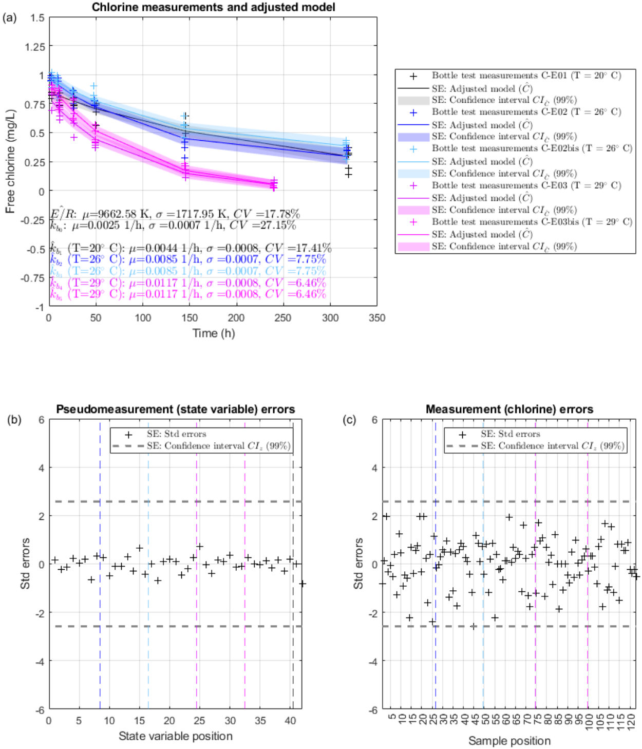
The ensemble temperature SE approach is now applied to grab samples C. Note that since free chlorine residual measured values do not reach zero for C-E01, C-E02 and C-E02bis, the assumed standard deviation for the final chlorine concentration has been increased to 0.5 mg/L in these tests as in the individual temperature analysis (Section 3.1.3). Three outliers are identified in this case (see Appendix A.2 for details). Figure 5 is equivalent to Figure 3 and Figure 4 once all outliers have been conveniently removed. The comparison between Figure A2 (in Appendix A.2) and Figure 5 shows that removing the outliers implies an increase in the mean and standard deviation of the activation coefficient (but a reduction in its CV) and a slight reduction in the mean of the bulk decay coefficient. In both Figure A2a and Figure 5a there is some degree of overlap for bottle tests at 20 °C (in gray) and 26 °C (in blues), with the temperature difference being more noticeable at 29 °C (purple/pink). Filtered results provide a mean value for the activation coefficient of 9662.58 K, a standard deviation of 1717.95 and a CV of 17.78%. The corresponding statistical properties for the reference bulk decay coefficient are 0.0025 1/h, 0.0007 1/h and 27.15%, respectively. This coefficient of variation is higher than for sources A and B, and similar to the average CV obtained with the individual temperature approach (24.53%). The most important aspect of the ensemble approach is that it ensures that the bulk decay coefficient always increases with temperature, i.e., SE results respect the Arrhenius formula (Equation (1)). This is key to systematizing the computation of the bulk decay coefficient (and so the wall contribution) at any position within the water supply network. Moreover, the ensemble approach lowers the coefficient of variation obtained for the bulk decay coefficient at different temperatures (6.46–17.41%, Figure 5a) compared to the individual approach (9.27–50.94%, see Table 7).

Figure 5. Ensemble temperature state estimation results for treatment works C (without outliers): (a) free chlorine residual measurements and adjusted first-order decay model, (b) standardized pseudomeasurement errors, and (c) standardized measurement errors.

4. Discussion

The ensemble temperature SE approach is presented here as an alternative methodology to the individual temperature SE approach introduced in Cejas et al. [27]. Results have shown that the ensemble approach provides a coefficient of variation for the reference bulk coefficient $k_{b_0}$ very similar in order of magnitude to that obtained when running the individual approach. However, the uncertainty of the bulk decay coefficient for bottle tests at different temperatures ($k_{b_j};\forall j=\mathrm{1,2},\dots ,n_T$) is lower with the ensemble approach due to the cross-correlation between $k_{b_0}$ and E/R. Apart from this reduction in uncertainty, the main advantage of the ensemble approach is that bulk decay coefficients are consistent among each other even when the temperature changes. This is an improvement because it ensures that the fundamental Arrhenius formula will be satisfied at any network position, i.e., bulk decay will be better characterized and consequently wall decay understanding will improve as well. The strong point of the ensemble formulation is that it enables us to jointly assess different bottle tests (with special interest in bottle tests subjected to different temperatures due to the relevance of temperature in the chlorine decay process), providing a systematic framework to assess uncertainty effects.

Results have shown that the ensemble approach presents special interest in waters with low TOC, which are typically associated with slow (and less defined) bulk decays. Table 8 summarizes the ensemble temperature SE approach results for bottle tests A, B and C (after removing outliers, i.e., Figure 3, Figure 4 and Figure 5). This table shows that the Arrhenius formula parameters (activation coefficient E/R and reference bulk decay coefficient $k_{b_0}$) vary widely (in mean, standard deviation and CV) for water samples from different sources. Note that Cohen’s distances (Equation (14)) are also computed in Table 8 to give an idea of how similar samples are among each other. Cohen’s ds are computed here for combinations A–B, A–C and B–C in terms of the two Arrhenius parameters. Cohen’s distances show that the reference bulk decay coefficient varies widely, as expected given the wide dispersion of bulk decay parameters previously described in the literature [8,27,42]. However, the probabilistic distribution of the activation coefficient changes less clearly among different grab samples. This reinforces the idea that assuming one a priori estimation of the activation coefficient (and high standard deviation) is reasonable (see Table 3). It also shows that Cohen’s d is a useful tool to assess the degree of similarity among distributions both for replications of the same bottle test (as discussed when presenting individual temperature SE results) and for comparison among different water samples (as illustrated in Table 8).

Table 8. Comparison of ensemble temperature state estimation results for bottle tests A, B and C.

State Variable		Grab Samples			Grab Sample Combinations
		A	B	C	A–B	A–C	B–C
Activation coefficient $\left(\widehat{E/R}\right)$	Mean $\mu$ (K)	7902.44	5164.41	9662.58	-	-	-
	Std $\sigma$ (K)	1102.50	1065.35	1717.95	-	-	-
	CV (%)	13.95	20.63	17.78	-	-	-
	Cohen’s d (−)	-	-	-	2.53	1.22	3.15
First-order reference bulk decay coefficient ${\widehat{k}}_{b_0}$	Mean $\mu$ (1/h)	0.0368	0.0097	0.0025	-	-	-
	Std $\sigma$ (1/h)	0.0052	0.0013	0.0007	-	-	-
	CV (%)	14.20	13.49	27.15	-	-	-
	Cohen’s d (−)	-	-	-	7.15	9.24	6.90

The ensemble temperature state estimation approach goes one step beyond previous approaches and ensures that there are no inconsistencies among free chlorine residual bulk decay coefficient values, with quantification of the associated uncertainty. In other words, the new method ensures that the bulk decay component is correctly characterized, and this has direct practical implications for the management of free chlorine residuals in water distribution networks. This approach can be applied to characterize the bulk decay component at any distribution network. As explained in the Introduction, the bulk decay component is typically characterized at the entrance to the network and considered constant throughout the system [26]. Therefore, once hydraulic results (i.e., velocities and thus residence times or water ages) and water temperatures (according to any available temperature engine, e.g., [17,25]) are known at each pipe, the free chlorine residual level according to a bulk decay model only can be obtained through the adjusted reference bulk decay and activation coefficients. Furthermore, there may be deviations between chlorine measurements and chlorine simulations according to the bulk decay model due to the wall effect. The wall effect, which coexists with bulk decay along a pipe network, may be characterized at a second stage by comparing chlorine measurements at different network positions with modeled values according to the first-order bulk decay model adjusted for different temperatures. Another question is if running the ensemble temperature SE approach to characterize bulk decay is truly needed at all networks. The answer is that it depends. Depending on the source water characteristics and the thermal amplitude in the network, it may be worth (or not) evaluating changes in the bulk decay coefficient. According to the Arrhenius formula (Equation (1)), if the activation coefficient and/or temperature gradients are low, it may not be worth going through the trouble/expense of characterizing the dependency with temperature. Improvements are still needed to monitor temperature at water supply networks [16] and/or implement robust temperature engines in hydraulic network calculations [17,25], but this paper provides a methodology to determine whether the sensitivity of the bulk decay coefficient will be high enough to care about temperature changes in the network. In a similar fashion, at the moment (and to the best of the authors’ knowledge) there is no explicit relationship between the bulk decay coefficient and other water quality parameters, e.g., TOC, ionic strength, specific ions, alkalinity. If any explicit relationships were derived for a specific case, the state estimation approach could be adapted to cope with these additional equation/s and compute the uncertainty of the corresponding parameters. Therefore, the ensemble temperature SE approach constitutes a tool (i.e., methodological contribution) to determine how important temperature modeling is in a specific network.

5. Conclusions

This work presents a new methodology (ensemble temperature state estimation approach) to compute Arrhenius equation parameters (reference bulk decay coefficient and activation coefficient) from bottle test data at different temperatures. This formulation constitutes an improvement with respect to previous works because it ensures the best possible fit of the Arrhenius equation considering the uncertainty of the bulk decay coefficient estimation process. The method has been applied in this work to water samples from different sources and temperatures, and bottle tests have been replicated to better understand the application possibilities of the methodology. This assessment has enabled us to identify Cohen’s distance as an interesting parameter to compare replicated bottle tests and/or water samples from different sources.

Results show that embracing the ensemble temperature SE approach implies a reduction in the standard deviation of the estimated bulk decay coefficients for bottle tests at different temperatures. Moreover, this approach represents an improvement with respect to previous works because it guarantees that bulk decay coefficients increase with temperature as expected based on evidence from the physical phenomenon itself. Uncertainty assessment is particularly important because it allows us to determine, based on the available measurements, whether Arrhenius parameters obtained for water samples from different sources are clearly different (or not). This helps us to understand the ranges of variation for both the reference bulk decay and activation coefficients (currently very wide according to the existing literature), which are determined by both the water source characteristics and the available measurements. Uncertainty analysis is also essential for identifying the experimental characteristics required in bottle tests (number of measurements, number of replications, bottle test temperatures, etc.) to achieve the desired level of certainty. Once both the mean and standard deviation of Arrhenius parameters are known (and as long as temperature through the water supply network is available, either measured or simulated), free chlorine residual values can be modeled (considering temperature) according to a bulk decay model only. This should improve the chances of better understanding and explaining the wall contribution to chlorine decay and quantifying the impacts of climate change on the management of water supply systems.

Appendix A.1. Free Chlorine Residual Measurements

Table A1 gathers free chlorine residual measurements over time for the five parallel bottle tests carried out with grab samples from sources A, B and C. Measurements for the first average time are represented in gray and are excluded for the $k_b$ analysis as explained in Cejas et al. [27]. The number of average times ($n_{{times}_j}$) is not the same for each water source nor for each temperature within the same source, due to differences in water characteristics and the dependence of chlorine decay on temperature. Furthermore, chlorine decays faster for sample A due to its higher TOC.

Table A1. Free chlorine residual measurements at three different temperatures (with replications) during parallel bottle tests for treatment works A, B and C. Measurements from the first average time are in gray and will be disregarded for the analyses (fast decay process, see [27]).

(a) Treatment Works A
	A-E01		A-E02		A-E02bis		A-E03		A-E03bis
Meas. No.	Avg. Time [h]	Free Chlorine Residual [mg/L]	Avg. Time [h]	Free Chlorine Residual [mg/L]	Avg. Time [h]	Free Chlorine Residual [mg/L]	Avg. Time [h]	Free Chlorine Residual [mg/L]	Avg. Time [h]	Free Chlorine Residual [mg/L]
-	-	-	-	-	1.15	0.73	1.10	0.94	-	-
-	0.97	0.82	1.10	0.63	1.15	0.71	1.10	0.68	1.13	0.76
-	0.97	0.89	1.10	0.72	1.15	0.68	1.10	0.80	1.13	0.88
-	0.97	0.84	1.10	0.72	1.15	0.81	1.10	0.82	1.13	0.69
-	0.97	0.89	1.10	0.77	1.15	0.76	1.10	0.70	1.13	0.71
1	3.03	0.67	3.03	0.53	2.90	0.58	3.05	0.42	3.17	0.51
2	3.03	0.75	3.03	0.54	2.90	0.71	3.05	0.50	3.17	0.51
3	3.03	0.81	3.03	0.53	2.90	0.57	3.05	0.57	3.17	0.61
4	3.03	0.63	3.03	0.65	2.90	0.57	3.05	0.54	3.17	0.55
5	6.87	0.62	3.03	0.52	2.90	0.61	3.05	0.48	6.42	0.36
6	6.87	0.53	6.00	0.42	5.63	0.44	6.67	0.45	6.42	0.39
7	6.87	0.63	6.00	0.40	5.63	0.52	6.67	0.40	6.42	0.32
8	6.87	0.73	6.00	0.36	5.63	0.34	6.67	0.37	6.42	0.34
9	6.87	0.47	6.00	0.49	5.63	0.49	6.67	0.35	9.12	0.19
10	9.72	0.42	6.00	0.37	5.63	0.48	9.47	0.18	9.12	0.28
11	9.72	0.45	8.75	0.28	8.42	0.33	9.47	0.17	9.12	0.27
12	9.72	0.48	8.75	0.16	8.42	0.32	9.47	0.10	9.12	0.28
13	9.72	0.36	8.75	0.31	8.42	0.34	9.47	0.16	12.84	0.18
14	9.72	0.52	8.75	0.30	8.42	0.35	13.15	0.19	12.84	0.26
15	13.42	0.44	8.75	0.26	12.02	0.24	13.15	0.18	12.84	0.18
16	13.42	0.38	12.40	0.23	12.02	0.25	13.15	0.14	12.84	0.19
17	13.42	0.33	12.40	0.16	12.02	0.25	13.15	0.14	23.60	0.02
18	13.42	0.49	12.40	0.22	12.02	0.23	23.92	0.02	23.60	0.06
19	24.08	0.31	12.40	0.22	22.85	0.06	23.92	0.05	23.60	0.02
20	24.08	0.21	23.20	0.09	22.85	0.10	23.92	0.08	23.60	0.07
21	24.08	0.24	23.20	0.11	22.85	0.05	23.92	0.02	-	-
22	24.08	0.12	23.20	0.02	22.85	0.05	-	-	-	-
23	24.08	0.27	23.20	0.04	-	-	-	-	-	-
24	47.53	0.03	23.20	0.04	-	-	-	-	-	-
25	47.53	0.11	-	-	-	-	-	-	-	-
26	47.53	0.04	-	-	-	-	-	-	-	-
27	47.53	0.02	-	-	-	-	-	-	-	-
(b) Treatment Works B
	B-E01		B-E02		B-E02bis		B-E03		B-E03bis
Meas. No.	Avg. time [h]	Free chlorine residual [mg/L]	Avg. time [h]	Free chlorine residual [mg/L]	Avg. time [h]	Free chlorine residual [mg/L]	Avg. time [h]	Free chlorine residual [mg/L]	Avg. time [h]	Free chlorine residual [mg/L]
-	1.05	0.61	1.15	0.87	1.07	0.93	1.03	0.80	1.10	0.82
-	1.05	0.62	1.15	0.72	1.07	0.83	1.03	0.80	1.10	0.82
-	1.05	0.65	1.15	0.67	1.07	0.83	1.03	0.85	1.10	0.89
-	1.05	0.60	1.15	0.78	1.07	0.87	1.03	0.79	1.10	0.85
1	3.08	0.69	3.15	0.70	2.93	0.68	3.13	0.61	3.18	0.67
2	3.08	0.70	3.15	0.87	2.93	0.75	3.13	0.62	3.18	0.72
3	3.08	0.67	3.15	0.63	2.93	0.75	3.13	0.70	3.18	0.82
4	3.08	0.58	3.15	0.63	2.93	0.73	3.13	0.69	3.18	0.71
5	11.23	0.55	10.25	0.55	9.90	0.65	10.95	0.55	10.58	0.54
6	11.23	0.59	10.25	0.47	9.90	0.60	10.95	0.48	10.58	0.58
7	11.23	0.57	10.25	0.49	9.90	0.62	10.95	0.41	10.58	0.63
8	11.23	0.46	10.25	0.50	9.90	0.60	10.95	0.57	10.58	0.52
9	24.18	0.46	24.05	0.46	24.27	0.66	23.92	0.36	24.08	0.42
10	24.18	0.42	24.05	0.47	24.27	0.59	23.92	0.36	24.08	0.34
11	24.18	0.48	24.05	0.55	24.27	0.49	23.92	0.30	24.08	0.43
12	24.18	0.43	24.05	0.43	24.27	0.46	23.92	0.30	24.08	0.43
13	50.02	0.29	49.23	0.29	24.27	0.48	49.75	0.23	49.48	0.30
14	50.02	0.32	49.23	0.31	48.90	0.36	49.75	0.20	49.48	0.33
15	50.02	0.29	49.23	0.33	48.90	0.35	49.75	0.25	49.48	0.39
16	50.02	0.30	49.23	0.26	48.90	0.36	49.75	0.18	49.48	0.36
17	144.68	0.14	143.92	0.05	48.90	0.29	144.42	0.07	144.12	0.02
18	144.68	0.10	143.92	0.13	143.67	0.10	144.42	0.02	144.12	0.03
19	144.68	0.10	143.92	0.02	143.67	0.11	144.42	0.05	144.12	0.02
20	144.68	0.12	143.92	0.05	143.67	0.09	144.42	0.02	144.12	0.02
21	224.06	0.08	-	-	143.67	0.08	-	-	-	-
22	224.06	0.08	-	-	-	-	-	-	-	-
23	224.06	0.06	-	-	-	-	-	-	-	-
24	224.06	0.02	-	-	-	-	-	-	-	-
(c) Treatment Works C
	C-E01		C-E02		C-E02bis		C-E03		C-E03bis
Meas. No.	Avg. time [h]	Free chlorine residual [mg/L]	Avg. time [h]	Free chlorine residual [mg/L]	Avg. time [h]	Free chlorine residual [mg/L]	Avg. time [h]	Free chlorine residual [mg/L]	Avg. time [h]	Free chlorine residual [mg/L]
-	1.08	0.95	0.82	1.00	1.03	0.97	1.05	0.87	1.08	0.97
-	1.08	0.91	0.82	1.03	1.03	0.99	1.05	0.88	1.08	0.98
-	1.08	0.92	0.82	1.01	1.03	1.02	1.05	0.84	1.08	0.95
-	1.08	0.98	0.82	1.10	1.03	0.98	1.05	0.86	1.08	0.96
1	3.10	0.79	2.47	0.94	3.30	0.94	3.07	0.69	3.08	0.87
2	3.10	0.85	2.47	0.95	3.30	1.02	3.07	0.88	3.08	0.91
3	3.10	0.97	2.47	0.97	3.30	0.89	3.07	0.83	3.08	0.91
4	3.10	0.82	2.47	0.99	3.30	0.98	3.07	0.84	3.08	0.88
5	11.08	0.81	9.78	0.94	9.25	0.99	10.98	0.61	10.42	0.76
6	11.08	0.78	9.78	0.97	9.25	0.79	10.98	0.74	10.42	0.86
7	11.08	0.84	9.78	0.82	9.25	0.96	10.98	0.70	10.42	0.88
8	11.08	0.73	9.78	0.94	9.25	0.92	10.98	0.72	10.42	0.70
9	26.77	0.85	25.48	0.75	24.92	0.85	10.98	0.64	26.08	0.79
10	26.77	0.80	25.48	0.85	24.92	0.82	26.60	0.66	26.08	0.61
11	26.77	0.71	25.48	0.71	24.92	0.87	26.60	0.58	26.08	0.62
12	26.77	0.74	25.48	0.86	24.92	0.87	26.60	0.46	26.08	0.78
13	26.77	0.73	48.62	0.78	48.02	0.90	26.60	0.58	49.22	0.44
14	49.86	0.56	48.62	0.77	48.02	0.78	49.75	0.37	49.22	0.51
15	49.86	0.75	48.62	0.74	48.02	0.82	49.75	0.44	49.22	0.57
16	49.86	0.51	48.62	0.73	48.02	0.79	49.75	0.41	49.22	0.42
17	49.86	0.68	144.65	0.25	144.08	0.57	49.75	0.39	49.22	0.57
18	49.86	0.74	144.65	0.42	144.08	0.56	145.48	0.18	145.00	0.21
19	145.58	0.56	144.65	0.37	144.08	0.46	145.48	0.11	145.00	0.38
20	145.58	0.64	144.65	0.28	144.08	0.64	145.48	0.21	145.00	0.21
21	145.58	0.49	317.83	0.37	317.10	0.40	145.48	0.15	145.00	0.23
22	145.58	0.64	317.83	0.35	317.10	0.30	240.32	0.02	239.37	0.04
23	319.10	0.31	317.83	0.30	317.10	0.27	240.32	0.06	239.37	0.03
24	319.10	0.19	317.83	0.34	317.10	0.41	240.32	0.07	239.37	0.04
25	319.10	0.32	-	-	317.10	0.43	240.32	0.09	239.37	0.02
26	319.10	0.14	-	-	-	-	-	-	-	-
27	319.10	0.37	-	-	-	-	-	-	-	-

Table A1. Free chlorine residual measurements at three different temperatures (with replications) during parallel bottle tests for treatment works A, B and C. Measurements from the first average time are in gray and will be disregarded for the analyses (fast decay process, see [27]).

(a) Treatment Works A
	A-E01		A-E02		A-E02bis		A-E03		A-E03bis
Meas. No.	Avg. Time [h]	Free Chlorine Residual [mg/L]	Avg. Time [h]	Free Chlorine Residual [mg/L]	Avg. Time [h]	Free Chlorine Residual [mg/L]	Avg. Time [h]	Free Chlorine Residual [mg/L]	Avg. Time [h]	Free Chlorine Residual [mg/L]
-	-	-	-	-	1.15	0.73	1.10	0.94	-	-
-	0.97	0.82	1.10	0.63	1.15	0.71	1.10	0.68	1.13	0.76
-	0.97	0.89	1.10	0.72	1.15	0.68	1.10	0.80	1.13	0.88
-	0.97	0.84	1.10	0.72	1.15	0.81	1.10	0.82	1.13	0.69
-	0.97	0.89	1.10	0.77	1.15	0.76	1.10	0.70	1.13	0.71
1	3.03	0.67	3.03	0.53	2.90	0.58	3.05	0.42	3.17	0.51
2	3.03	0.75	3.03	0.54	2.90	0.71	3.05	0.50	3.17	0.51
3	3.03	0.81	3.03	0.53	2.90	0.57	3.05	0.57	3.17	0.61
4	3.03	0.63	3.03	0.65	2.90	0.57	3.05	0.54	3.17	0.55
5	6.87	0.62	3.03	0.52	2.90	0.61	3.05	0.48	6.42	0.36
6	6.87	0.53	6.00	0.42	5.63	0.44	6.67	0.45	6.42	0.39
7	6.87	0.63	6.00	0.40	5.63	0.52	6.67	0.40	6.42	0.32
8	6.87	0.73	6.00	0.36	5.63	0.34	6.67	0.37	6.42	0.34
9	6.87	0.47	6.00	0.49	5.63	0.49	6.67	0.35	9.12	0.19
10	9.72	0.42	6.00	0.37	5.63	0.48	9.47	0.18	9.12	0.28
11	9.72	0.45	8.75	0.28	8.42	0.33	9.47	0.17	9.12	0.27
12	9.72	0.48	8.75	0.16	8.42	0.32	9.47	0.10	9.12	0.28
13	9.72	0.36	8.75	0.31	8.42	0.34	9.47	0.16	12.84	0.18
14	9.72	0.52	8.75	0.30	8.42	0.35	13.15	0.19	12.84	0.26
15	13.42	0.44	8.75	0.26	12.02	0.24	13.15	0.18	12.84	0.18
16	13.42	0.38	12.40	0.23	12.02	0.25	13.15	0.14	12.84	0.19
17	13.42	0.33	12.40	0.16	12.02	0.25	13.15	0.14	23.60	0.02
18	13.42	0.49	12.40	0.22	12.02	0.23	23.92	0.02	23.60	0.06
19	24.08	0.31	12.40	0.22	22.85	0.06	23.92	0.05	23.60	0.02
20	24.08	0.21	23.20	0.09	22.85	0.10	23.92	0.08	23.60	0.07
21	24.08	0.24	23.20	0.11	22.85	0.05	23.92	0.02	-	-
22	24.08	0.12	23.20	0.02	22.85	0.05	-	-	-	-
23	24.08	0.27	23.20	0.04	-	-	-	-	-	-
24	47.53	0.03	23.20	0.04	-	-	-	-	-	-
25	47.53	0.11	-	-	-	-	-	-	-	-
26	47.53	0.04	-	-	-	-	-	-	-	-
27	47.53	0.02	-	-	-	-	-	-	-	-
(b) Treatment Works B
	B-E01		B-E02		B-E02bis		B-E03		B-E03bis
Meas. No.	Avg. time [h]	Free chlorine residual [mg/L]	Avg. time [h]	Free chlorine residual [mg/L]	Avg. time [h]	Free chlorine residual [mg/L]	Avg. time [h]	Free chlorine residual [mg/L]	Avg. time [h]	Free chlorine residual [mg/L]
-	1.05	0.61	1.15	0.87	1.07	0.93	1.03	0.80	1.10	0.82
-	1.05	0.62	1.15	0.72	1.07	0.83	1.03	0.80	1.10	0.82
-	1.05	0.65	1.15	0.67	1.07	0.83	1.03	0.85	1.10	0.89
-	1.05	0.60	1.15	0.78	1.07	0.87	1.03	0.79	1.10	0.85
1	3.08	0.69	3.15	0.70	2.93	0.68	3.13	0.61	3.18	0.67
2	3.08	0.70	3.15	0.87	2.93	0.75	3.13	0.62	3.18	0.72
3	3.08	0.67	3.15	0.63	2.93	0.75	3.13	0.70	3.18	0.82
4	3.08	0.58	3.15	0.63	2.93	0.73	3.13	0.69	3.18	0.71
5	11.23	0.55	10.25	0.55	9.90	0.65	10.95	0.55	10.58	0.54
6	11.23	0.59	10.25	0.47	9.90	0.60	10.95	0.48	10.58	0.58
7	11.23	0.57	10.25	0.49	9.90	0.62	10.95	0.41	10.58	0.63
8	11.23	0.46	10.25	0.50	9.90	0.60	10.95	0.57	10.58	0.52
9	24.18	0.46	24.05	0.46	24.27	0.66	23.92	0.36	24.08	0.42
10	24.18	0.42	24.05	0.47	24.27	0.59	23.92	0.36	24.08	0.34
11	24.18	0.48	24.05	0.55	24.27	0.49	23.92	0.30	24.08	0.43
12	24.18	0.43	24.05	0.43	24.27	0.46	23.92	0.30	24.08	0.43
13	50.02	0.29	49.23	0.29	24.27	0.48	49.75	0.23	49.48	0.30
14	50.02	0.32	49.23	0.31	48.90	0.36	49.75	0.20	49.48	0.33
15	50.02	0.29	49.23	0.33	48.90	0.35	49.75	0.25	49.48	0.39
16	50.02	0.30	49.23	0.26	48.90	0.36	49.75	0.18	49.48	0.36
17	144.68	0.14	143.92	0.05	48.90	0.29	144.42	0.07	144.12	0.02
18	144.68	0.10	143.92	0.13	143.67	0.10	144.42	0.02	144.12	0.03
19	144.68	0.10	143.92	0.02	143.67	0.11	144.42	0.05	144.12	0.02
20	144.68	0.12	143.92	0.05	143.67	0.09	144.42	0.02	144.12	0.02
21	224.06	0.08	-	-	143.67	0.08	-	-	-	-
22	224.06	0.08	-	-	-	-	-	-	-	-
23	224.06	0.06	-	-	-	-	-	-	-	-
24	224.06	0.02	-	-	-	-	-	-	-	-
(c) Treatment Works C
	C-E01		C-E02		C-E02bis		C-E03		C-E03bis
Meas. No.	Avg. time [h]	Free chlorine residual [mg/L]	Avg. time [h]	Free chlorine residual [mg/L]	Avg. time [h]	Free chlorine residual [mg/L]	Avg. time [h]	Free chlorine residual [mg/L]	Avg. time [h]	Free chlorine residual [mg/L]
-	1.08	0.95	0.82	1.00	1.03	0.97	1.05	0.87	1.08	0.97
-	1.08	0.91	0.82	1.03	1.03	0.99	1.05	0.88	1.08	0.98
-	1.08	0.92	0.82	1.01	1.03	1.02	1.05	0.84	1.08	0.95
-	1.08	0.98	0.82	1.10	1.03	0.98	1.05	0.86	1.08	0.96
1	3.10	0.79	2.47	0.94	3.30	0.94	3.07	0.69	3.08	0.87
2	3.10	0.85	2.47	0.95	3.30	1.02	3.07	0.88	3.08	0.91
3	3.10	0.97	2.47	0.97	3.30	0.89	3.07	0.83	3.08	0.91
4	3.10	0.82	2.47	0.99	3.30	0.98	3.07	0.84	3.08	0.88
5	11.08	0.81	9.78	0.94	9.25	0.99	10.98	0.61	10.42	0.76
6	11.08	0.78	9.78	0.97	9.25	0.79	10.98	0.74	10.42	0.86
7	11.08	0.84	9.78	0.82	9.25	0.96	10.98	0.70	10.42	0.88
8	11.08	0.73	9.78	0.94	9.25	0.92	10.98	0.72	10.42	0.70
9	26.77	0.85	25.48	0.75	24.92	0.85	10.98	0.64	26.08	0.79
10	26.77	0.80	25.48	0.85	24.92	0.82	26.60	0.66	26.08	0.61
11	26.77	0.71	25.48	0.71	24.92	0.87	26.60	0.58	26.08	0.62
12	26.77	0.74	25.48	0.86	24.92	0.87	26.60	0.46	26.08	0.78
13	26.77	0.73	48.62	0.78	48.02	0.90	26.60	0.58	49.22	0.44
14	49.86	0.56	48.62	0.77	48.02	0.78	49.75	0.37	49.22	0.51
15	49.86	0.75	48.62	0.74	48.02	0.82	49.75	0.44	49.22	0.57
16	49.86	0.51	48.62	0.73	48.02	0.79	49.75	0.41	49.22	0.42
17	49.86	0.68	144.65	0.25	144.08	0.57	49.75	0.39	49.22	0.57
18	49.86	0.74	144.65	0.42	144.08	0.56	145.48	0.18	145.00	0.21
19	145.58	0.56	144.65	0.37	144.08	0.46	145.48	0.11	145.00	0.38
20	145.58	0.64	144.65	0.28	144.08	0.64	145.48	0.21	145.00	0.21
21	145.58	0.49	317.83	0.37	317.10	0.40	145.48	0.15	145.00	0.23
22	145.58	0.64	317.83	0.35	317.10	0.30	240.32	0.02	239.37	0.04
23	319.10	0.31	317.83	0.30	317.10	0.27	240.32	0.06	239.37	0.03
24	319.10	0.19	317.83	0.34	317.10	0.41	240.32	0.07	239.37	0.04
25	319.10	0.32	-	-	317.10	0.43	240.32	0.09	239.37	0.02
26	319.10	0.14	-	-	-	-	-	-	-	-
27	319.10	0.37	-	-	-	-	-	-	-	-

Appendix A.2. Ensemble Temperature State Estimation Approach (Before Removing Outliers)

This Appendix also includes ensemble temperature SE approach results for grab samples B and C before removing the outliers. Figure A1 is equivalent to Figure 3 for grab samples B. Figure A1a,c show that there is one outlier, which corresponds to measurement 2 in B-E02, as was already identified in the individual analysis. Figure 4 updates Figure A1 by removing this outlier from the analysis. Figure A2 is equivalent to Figure 3 for grab samples C. According to Figure A2a,c, there are three outliers: measurement 16 in C-E01, measurement 17 in C-E02 and measurement 19 in C-E03bis. This is one outlier more than that obtained in the individual analysis (only C-E01 and C-E03bis). Figure 5 updates Figure A2 by removing the three outliers.

Figure A1. Ensemble temperature state estimation results for treatment works B: (a) free chlorine residual measurements and adjusted first-order decay model, (b) standardized pseudomeasurement errors, and (c) standardized measurement errors.

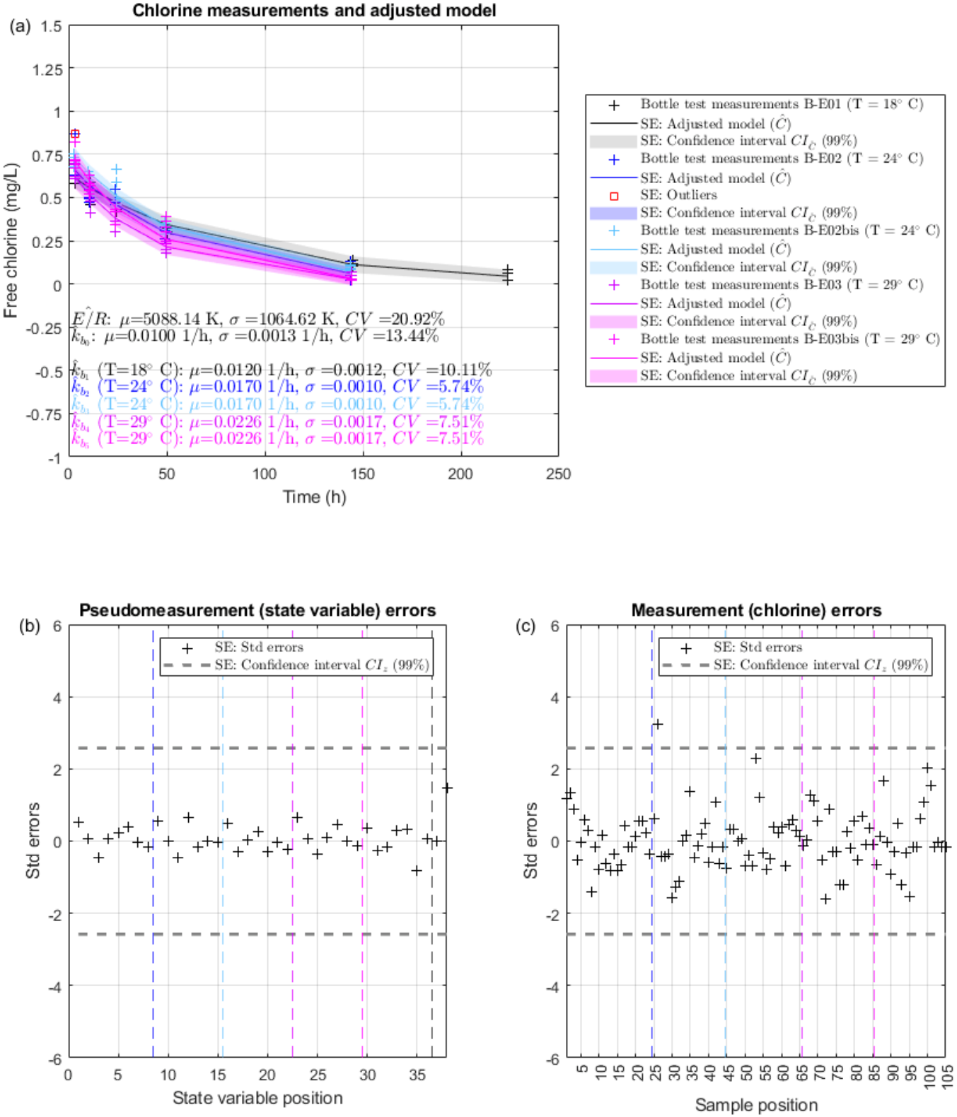
Figure A1. Ensemble temperature state estimation results for treatment works B: (a) free chlorine residual measurements and adjusted first-order decay model, (b) standardized pseudomeasurement errors, and (c) standardized measurement errors.

Figure A2. Ensemble temperature state estimation results for treatment works C: (a) free chlorine residual measurements and adjusted first-order decay model, (b) standardized pseudomeasurement errors, and (c) standardized measurement errors.

Figure A2. Ensemble temperature state estimation results for treatment works C: (a) free chlorine residual measurements and adjusted first-order decay model, (b) standardized pseudomeasurement errors, and (c) standardized measurement errors.

References

- Fish, K.E.; Reeves-McLaren, N.; Husband, S.; Boxall, J. Uncharted waters: The unintended impacts of residual chlorine on water quality and biofilms. npj Biofilms Microbiomes 2020, 6, 34. [Google Scholar] [CrossRef] [Scilit]
- Onyutha, S.; Kwio-Tamale, J.C. Modelling chlorine residuals in drinking water: A review. Int. J. Environ. Sci. Technol. 2022, 19, 11613–11630. [Google Scholar] [CrossRef] [Scilit]
- Ma, C.; Shi, W.; Wang, L.; Zhao, X.; Zhao, B.; Guo, X.; Zhang, Z.; Zhang, H. Effect of disinfection method on odor and disinfection byproduct control in drinking water treatment. Desalin. Water Treat. 2016, 57, 7753–7762. [Google Scholar] [CrossRef] [Scilit]
- WHO. Principles and Practices of Drinking-Water Chlorination; A Guide to strengthening Chlorination Practices in Small- to Medium-Sized Water Supplies; World Health Organization: Geneva, Switzerland, 2017. [Google Scholar]
- WHO. Guidelines for Drinking Water Quality; 4th Edition Incorporating the 1st and 2nd Addenda; World Health Organization: Geneva, Switzerland, 2022. [Google Scholar]
- Feben, D.; Taras, M.J. Studies on chlorine demand constants. J. Am. Water Work. Assoc. 1951, 43, 922–932. [Google Scholar] [CrossRef] [Scilit]
- Jadas-Hécart, A.; El Morer, A.; Stitou, M.; Buillot, P.; Legube, B. The chlorine demand of a treated water. Water Res. 1992, 26, 1073–1084. [Google Scholar] [CrossRef] [Scilit]
- Vasconcelos, J.J.; Rossman, L.A.; Grayman, W.M.; Boulos, P.F.; Clark, R.M. Kinetics of chlorine decay. J. Am. Water Work. Assoc. 1997, 89, 54–65. [Google Scholar] [CrossRef] [Scilit]
- Powell, J.C.; Hallam, N.B.; West, J.R.; Forster, C.F.; Simms, J. Factors which control bulk chlorine decay rates. Water Res. 2000, 34, 117–126. [Google Scholar] [CrossRef] [Scilit]
- Fisher, I.; Kastl, G.; Sathasivan, A. A suitable model of combined effects of temperature and initial condition on chlorine bulk decay in water distribution systems. Water Res. 2012, 46, 3293–3303. [Google Scholar] [CrossRef] [Scilit] [PubMed]
- Zhang, X.; Li, Y.; Chen, J.; Wang, H. Effects of heating temperature and water age on the formation of disinfection by-products in drinking water. Environ. Sci. Water Res. Technol. 2025, 11, 1285–1295. [Google Scholar] [CrossRef] [Scilit]
- Fogler, H.S. Elements of Chemical Reaction Engineering, 5th ed.; Prentice Hall: Hoboken, NJ, USA, 2016. [Google Scholar]
- Blokker, M.; Vreeburg, J.; Speight, V. Residual chlorine in the extremities of the drinking water distribution system: The influence of stochastic water demands. Procedia Eng. 2014, 70, 172–180. [Google Scholar] [CrossRef] [Scilit]
- Díaz, S.; González, J. The importance of water temperature in water supply systems. Ing. Del Agua 2022, 26, 107–123. (In Spanish) [Google Scholar] [CrossRef] [Scilit]
- Furst, K.E.; Graham, K.E.; Weisman, R.J.; Adusei, K.B. It’s getting hot in here: Effects of heat on temperature, disinfection, and opportunistic pathogens in drinking water distribution systems. Water Res. 2024, 260, 121913. [Google Scholar] [CrossRef] [Scilit]
- Agudelo-Vera, C.; Avvedimento, S.; Boxall, J.; Creaco, E.; de Kater, H.; Di Nardo, A.; Djukic, A.; Douterelo, I.; Fish, K.E.; Iglesias-Rey, P.L.; et al. Drinking water temperature around the globe: Undertansing, Policies, challenges and opportunities. Water 2020, 12, 1049. [Google Scholar] [CrossRef] [Scilit]
- Díaz, S.; Boxall, J.; Lamarche, L.; González, J. The impact of ground heat capacity on drinking water temperature. J. Water Resour. Plan. Manag. 2023, 149, 04023012. [Google Scholar] [CrossRef] [Scilit]
- van Summeren, J.; Raterman, B.; Vonk, E.; Blokker, M.; van Erp, J.; Vries, D. Influence of temperature, network diagnostics, and demographic factors on discoloration-related customer reports. Procedia Eng. 2015, 119, 416–425. [Google Scholar] [CrossRef] [Scilit]
- Cook, D.; Husband, S.; Boxall, J. Operational management of trunk main discolouration risk. Urban Water J. 2015, 13, 382–395. [Google Scholar] [CrossRef] [Scilit]
- Calero, C.; Boxall, J.; Soria-Carrasco, V.; Martínez, S.; Douterelo, I. Implications of climate change: How does increased water temperature influence biofilm and water quality of chlorinated drinking water distribution systems? Front. Microbiol. 2021, 12, 658927. [Google Scholar] [CrossRef] [Scilit]
- Blokker, M.; Pieterse-Quirijns, E. Modeling temperature in the drinking water distribution system. J. Am. Water Work. Assoc. 2013, 105, 19–28. [Google Scholar] [CrossRef] [Scilit]
- De Pasquale, A.M.; Giostri, A.; Romano, M.C.; Chiesa, P.; Demeco, T.; Tani, S. District heating by drinking water heat pump: Modelling and energy analysis of a case study in the city of Milan. Energy 2017, 118, 246–263. [Google Scholar] [CrossRef] [Scilit]
- Hubeck-Graudal, H.; Kirstein, J.K.; Ommen, T.; Rygaard, M.; Elmegaard, B. Drinking water supply as low-temperature source in the district heating system: A case study for the city of Copenhagen. Energy 2020, 194, 116773. [Google Scholar] [CrossRef] [Scilit]
- Hypolite, G.; Ferrasse, J.H.; Boutin, O.; del Sole, S.; Cloarec, J.F. Dynamic modeling of water temperature and flow in large water system. Appl. Therm. Eng. 2021, 196, 117261. [Google Scholar] [CrossRef] [Scilit]
- Blokker, M.; Pan, Q.; van Laarhoven, K. Validation of an enhanced drinking water temperature model during distribution. Water 2024, 16, 2796. [Google Scholar] [CrossRef] [Scilit]
- Vieira, P.; Coelho, S.T.; Loureiro, D. Accounting for the influence of initial chlorine concentration, TOC, iron and temperature when modelling chlorine decay in water supply. J. Water Supply Res. Technol.–AQUA 2004, 53, 453–467. [Google Scholar] [CrossRef] [Scilit]
- Cejas, E.; Díaz, S.; González, J. Bottle test free chlorine bulk decay coefficient statistical fitting for water supply systems via state estimation techniques. Water 2025, 17, 2990. [Google Scholar] [CrossRef] [Scilit]
- Fisher, I.; Kastl, G.; Sathasivan, A. Evaluation of suitable chlorine bulk-decay models for water distribution systems. Water Res. 2011, 45, 4896–4908. [Google Scholar] [CrossRef] [Scilit]
- Fawzer, M.F.; Kastl, G.; Krishna, K.C.B.; Fisher, I.; Sathasivan, A. Bulk water microbes could accelerate chlorine decay at low chlorine concentrations. Water 2025, 17, 624. [Google Scholar] [CrossRef] [Scilit]
- Monteiro, L.; Figuereido, D.; Covas, D.; Menaia, J. Integrating water temperature in chlorine decay modelling: A case study. Urban Water J. 2017, 14, 1097–1101. [Google Scholar] [CrossRef] [Scilit]
- Kennedy, L.C.; Miller, S.E.; Kantor, R.S.; Nelson, K.L. Effect of disinfectant residual, pH, and temperature on microbial abundance in disinfected drinking water distribution systems. Environ. Sci. Water Res. Technol. 2021, 7, 78–92. [Google Scholar] [CrossRef] [Scilit]
- Hallam, H.B.; West, J.R.; Forster, C.F.; Simms, J. The potential for biofilm growth in water distribution systems. Water Res. 2001, 35, 4063–4071. [Google Scholar] [CrossRef] [Scilit] [PubMed]
- Pick, F.C.; Fish, K.E.; Husband, S.; Boxall, J.B. Non-invasive biofouling monitoring to assess drinking water distribution system performance. Front. Microbiol. 2021, 12, 730344. [Google Scholar] [CrossRef] [Scilit] [PubMed]
- McNeill, L.S.; Edwards, M. Iron pipe corrosion in distribution systems. J. Am. Water Work. Assoc. 2001, 93, 88–100. [Google Scholar] [CrossRef] [Scilit]
- McNeill, L.S.; Edwards, M. The importance of temperature in assessing iron pipe corrosion in water distribution systems. Environ. Monit. Assess. 2002, 77, 229–242. [Google Scholar] [CrossRef] [Scilit]
- Jun, H.J.; Park, J.K.; Bae, C.H. Factors affecting steel water-transmission pipe failure and pipe-failure mechanisms. J. Environ. Eng. 2020, 146, 04020034. [Google Scholar] [CrossRef] [Scilit]
- Coulson, J.M.; Richardson, F.J. Chemical Engineering, 2nd ed.; Pergamon Press: Oxford, UK, 1964. [Google Scholar]
- Schweppe, F.C.; Wildes, J. Power system static state estimation. Part I: Exact model. IEEE Trans. Power Appar. Syst. 1970, 89, 120–125. [Google Scholar] [CrossRef] [Scilit]
- Abur, A.; Expósito, A.G. Electric Power System State Estimation; Theory and Implementations; Marcel Dekker: New York, NY, USA, 2004. [Google Scholar]
- Díaz, S.; González, J.; Mínguez, R. Observability analysis in water transport networks: Algebraic approach. J. Water Resour. Plan. Manag. 2015, 142, 04015071. [Google Scholar] [CrossRef] [Scilit]
- Ruiz, E.; Díaz, S.; González, J. State variable implications on hydraulic state estimation. Water Resour. Manag. 2022, 36, 2549–2569. [Google Scholar] [CrossRef] [Scilit]
- Speight, V.; Boxall, J. Current perspectives on disinfectant modelling. Procedia Eng. 2015, 119, 434–441. [Google Scholar] [CrossRef] [Scilit]
- Kohpaei, A.J.; Sathasivan, A.; Aboutalebi, H. Evaluation of second order and parallel second order approaches to model temperature variation in chlorine decay modelling. Desalin. Water Treat. 2011, 32, 100–106. [Google Scholar] [CrossRef] [Scilit]
- Díaz, S.; González, J.; Mínguez, J. Uncertainty evaluation for constrained state estimation in water distribution systems. J. Water Resour. Plan. Manag. 2016, 142, 06016004. [Google Scholar] [CrossRef] [Scilit]
- Díaz, S.; Mínguez, R.; González, J. Probabilistic leak detectability assessment via state estimation in water transport networks. Stoch. Environ. Res. Risk Assess. 2018, 32, 2111–2128. [Google Scholar] [CrossRef] [Scilit]
- Bargiela, A.; Hainsworth, D. Pressure and flow uncertainty in water systems. J. Water Resour. Plan. Manag. 1989, 115, 212–229. [Google Scholar] [CrossRef] [Scilit]
- ISO 7393-1:2000; Water Quality. Determination of Free Chlorine and Total Chlorine. Part 1: Titrimetric Method Using N,N-diethyl-1,4-phenylenediamine. AENOR: Madrid, Spain, 2000; (In Spanish). Available online: https://tienda.aenor.com/p/norma-une-en-iso-7393-1-2000-n0023489 (accessed on 2 June 2026).
- Fundación Canal. Drinking Water Disinfection Treatment. 2005. (In Spanish) Available online: https://www.fundacioncanal.com/canaleduca/wp-content/uploads/2015/08/Tratamiento-de-desinfeccion-del-agua-potable2.pdf (accessed on 17 February 2025).
- European Comission. Directive (EU) 2020/2184 of the European Parliament and of the Council of 16 December 2020 on the Quality of Water Intended for Human Consumption. 2020. Available online: https://eur-lex.europa.eu/eli/dir/2020/2184/oj (accessed on 14 May 2026).
- Cohen, J. Statistical Power Analysis for the Behavioral Sciences, 2nd ed.; Lawrence Erlbaum Associates: New York, NY, USA, 1988. [Google Scholar]
Disclaimer/Publisher’s Note: The statements, opinions and data contained in all publications are solely those of the individual author(s) and contributor(s) and not of MDPI and/or the editor(s). MDPI and/or the editor(s) disclaim responsibility for any injury to people or property resulting from any ideas, methods, instructions or products referred to in the content. |
© 2026 by the authors. Licensee MDPI, Basel, Switzerland. This article is an open access article distributed under the terms and conditions of the Creative Commons Attribution (CC BY) license.