Decomposition–Migration Cooperative Modeling Approach for Forecasting Runoff in Data-Scarce Watershed Areas

Abstract

To address runoff forecasting inaccuracies caused by data gaps in reservoir operations, this paper proposes a collaborative modeling framework integrating deep learning, signal decomposition, uncertainty quantification, and transfer learning. Validated on the Wei River (source basin) and Yongding River (target basin) with similar hydrological characteristics, the framework first constructs a Pyraformer-BiLSTM-LSS point forecasting model to enhance characterization of non-stationary runoff sequences. Then, the BLSO-VMD optimization decomposition technique filters and reconstructs forecasting noise, improving model robustness. Subsequently, a probabilistic interval forecasting model is developed via multi-task learning to reliably quantify uncertainty. To tackle data scarcity in the target domain, a “decomposition–reconstruction–transfer” learning mechanism transfers model knowledge from the source domain to the target domain. Results show that the framework achieves excellent performance in the source domain and successfully transfers to the data-scarce target domain, significantly enhancing the accuracy and stability of both point and interval forecasts. By establishing a collaborative modeling framework combining transfer learning and multi-task learning, along with an adaptive signal decomposition method based on BLSO and a multi-scale deep learning model, this study effectively addresses the challenges of accuracy and reliability in runoff forecasting for data-scarce basins. It provides a transferable and scalable technical pathway for runoff simulation and reservoir operation in hydrologically underserved regions, supporting sustainable water resource management and ecological protection.

1. Introduction

China possesses abundant total water resources, but due to uneven spatial and temporal distribution, per capita availability remains far below the global average. Water scarcity has thus become a critical factor constraining sustainable socioeconomic development [1]. As a region with sparse data, the Yongding River Basin faces limitations in real-time flow monitoring. The limited amount of hydrological data available within the basin, coupled with its lack of timeliness and accuracy, results in severely inadequate forecasting accuracy of hydrological models, which significantly undermines the scientific basis of operational decisions and water resources management [2]. Under the dual impacts of global climate change and intensive human activities, the basin’s hydrological conditions have grown increasingly complex, with frequent extreme hydrological events posing significant challenges to traditional water resource management models [3,4]. Therefore, developing high-precision runoff forecasting techniques to enable scientific prediction and dynamic regulation of water resources in this basin holds major practical significance for safeguarding regional water security and supporting ecological civilization construction.

Runoff forecasting serves as a crucial foundation for water resources management, providing essential support for ecological regulation, flood control and disaster mitigation, and water resource allocation. To enhance forecasting accuracy, numerous scholars have introduced techniques such as time series decomposition (e.g., VMD, CEEMDAN) and intelligent optimization (e.g., genetic algorithms, particle swarm optimization) to improve traditional models [5,6,7]. With the rise of deep learning, complex neural network models (such as Pyraformer) have been extensively introduced into the field of hydrological forecasting, demonstrating superior performance [8,9,10,11]. However, traditional hydrological models rely heavily on extensive observational data and finely tuned parameters, often proving inadequate in data-scarce basins.

In recent years, to overcome the constraints imposed by data scarcity on hydrological modeling, transfer learning techniques have garnered increasing attention within the hydrology community [12,13,14]. Transfer learning has been introduced to the hydrological field with the aim of transferring knowledge acquired from data-rich source basins to data-scarce target basins, thereby enhancing forecasting performance. While this method is relatively mature in fields such as computer vision, it remains in its preliminary exploratory phase within hydrology [15]. Its core concept involves transferring knowledge and model features trained on data-rich “source basins” to data-poor “target basins,” thereby leveraging the informational advantages of larger basins to compensate for the data limitations of smaller ones [16,17]. Early research primarily focused on similarity-based parameter regionalization methods, which suffer from high subjectivity and limited accuracy [18]. With the advancement of deep learning, neural network-based transfer learning has demonstrated greater potential. Recent domestic studies have further explored methods such as selecting source basins based on geographic similarity criteria and incorporating semi-supervised learning to enhance transfer robustness, thereby improving application effectiveness in data-scarce regions [19,20,21]. These findings demonstrate that transfer learning can effectively leverage regional hydrological commonalities to mitigate modeling challenges caused by data scarcity. However, excessive feature differences between source and target basins may induce “negative transfer.” Current research remains in its infancy, with areas such as source basin selection, multi-source information fusion, and physical mechanism constraints requiring further refinement.

Addressing the core bottlenecks of insufficient robustness and generalization capabilities in runoff forecasting models under complex scenarios, as well as data scarcity in the Yongding River basin, this study systematically constructs a deep transfer learning “decomposition–reconstruction–transfer” forecasting framework that integrates hydrological–physical cognition. The Wei River basin, selected for its similar hydrological conditions and abundant data, serves as the source basin. The deep learning model is trained on Wei River basin data, with fine-tuning applied to its fully connected layers and output layer to rapidly adapt to the characteristics of the Yongding River basin. Under limited data conditions, this approach significantly enhances the accuracy and robustness of runoff forecasting for the Yongding River basin, providing a replicable, theoretically grounded technical solution for hydrological forecasting in similarly data-scarce regions.

2. Study Area and Data Sources

2.1. Study Area

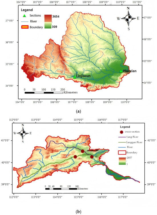
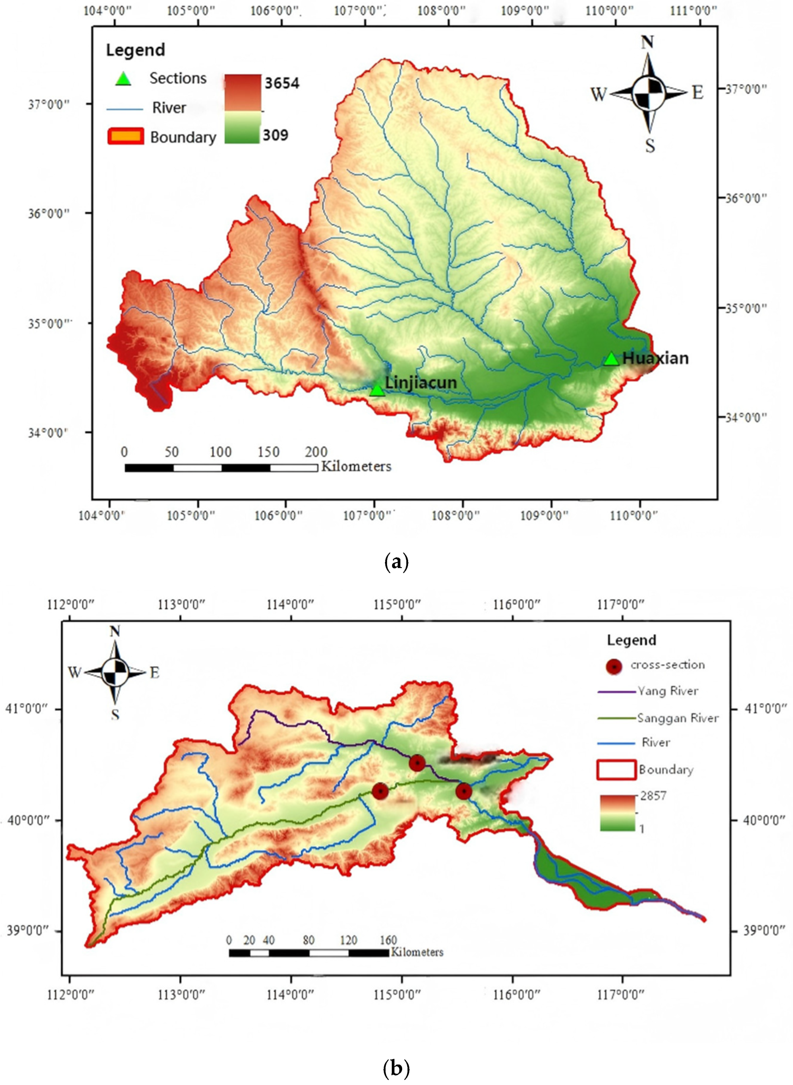
This study selected the Wei River (source basin) and Yongding River (target basin) as research subjects [22,23]. The Wei River, the largest tributary of the Yellow River, spans 818 km in length with a catchment area of approximately 13.5 × 104 km². Flowing through multiple provinces including Gansu and Shaanxi, its upper reaches are situated in the Loess Hills region characterized by complex hydrological and climatic conditions, making it an ideal area for runoff simulation studies. The Yongding River is one of the major rivers in the Haihe River Basin, with a total catchment area of approximately 4.70 × 104 km², where mountainous terrain accounts for 95.8%. Sanjiadian serves as the boundary between its mountainous and plain sections.

The Wei River and Yongding River exhibit strong similarities in geographical and hydrological characteristics, providing a foundation for inter-basin data transfer. Both rivers are situated in China’s northern semi-arid to semi-humid monsoon climate zone, where precipitation is concentrated in summer with frequent torrential rains. Precipitation and evaporation show pronounced seasonal fluctuations, resulting in concentrated summer runoff and sharp winter reductions. Topographically, both basins exhibit a “mountainous–plains” transition: the Wei River traverses loess hills and alluvial plains, while the Yongding River primarily flows through mountainous terrain before entering plains in its lower reaches. Mountainous areas exhibit rapid runoff response with pronounced flood peaks, whereas plains show relatively gradual runoff patterns. Regarding hydrological events, both rivers are prone to torrential rain-induced floods characterized by sudden onset, short duration, high sediment content, and pronounced flood peak fluctuations. Their flood formation mechanisms and response patterns are largely consistent. Ecologically, both basins face issues of overexploited water resources: the Guanzhong section of the Wei River suffers from pollution pressures, while the Beijing section of the Yongding River frequently experiences water stoppages. Both rivers exhibit pronounced seasonal concentration in runoff, with June to September accounting for over 70% of annual discharge.

Additionally, they share several water conservancy measures: both river basins have large-scale backbone reservoirs (such as the Dongzhuang and Jinpen hubs on the Wei River and the Guanting Reservoir on the Yongding River) serving multiple functions including flood control and water supply; both have implemented large-scale embankment construction and river channel regulation projects, significantly raising flood control standards; and both have established water diversion irrigation or inter-basin water replenishment systems (such as the Baojixia Wei River Diversion Irrigation District on the Wei River and the Yellow River water replenishment project on the Yongding River), and have in recent years vigorously promoted ecological restoration and comprehensive management projects. The similarity between the Wei River and the Yongding River provides a crucial foundation for conducting transfer learning across river basins.

The geographical location of the study area is shown in Figure 1.

Figure 1. Geographical location map of the study area: (a) Wei River Basin, (b) Yongding River Basin.

2.2. Data Sources

This study collected daily runoff data from 1 January 1997 to 1 May 2020, for the source domain of the Wei River Basin in Huaxian County. To thoroughly analyze the hydrological processes in the Wei River Basin, the research selected multiple meteorological and hydrological variables, including precipitation, potential evapotranspiration, relative humidity, sunshine duration, daily mean temperature, daily maximum temperature, daily minimum temperature, and wind speed. All data were sourced from meteorological records provided by the National Meteorological Information Center and hydrological data from the National Real-time Rainfall and Water Conditions Database. Concurrently, daily runoff data from 1 January 2020 to 31 December 2020, were collected for three key cross-sections of the target Yongding River basin: Guanting, Shixiali, and Xiangshuipu. The study indicates that transfer learning yields the most significant benefits when the daily-scale sample size is <800.

3. Methods

3.1. A Data-Sparse Runoff Forecasting Framework Based on Decomposition–Transition Synergistic Modeling

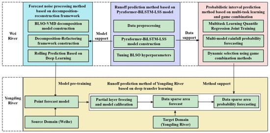
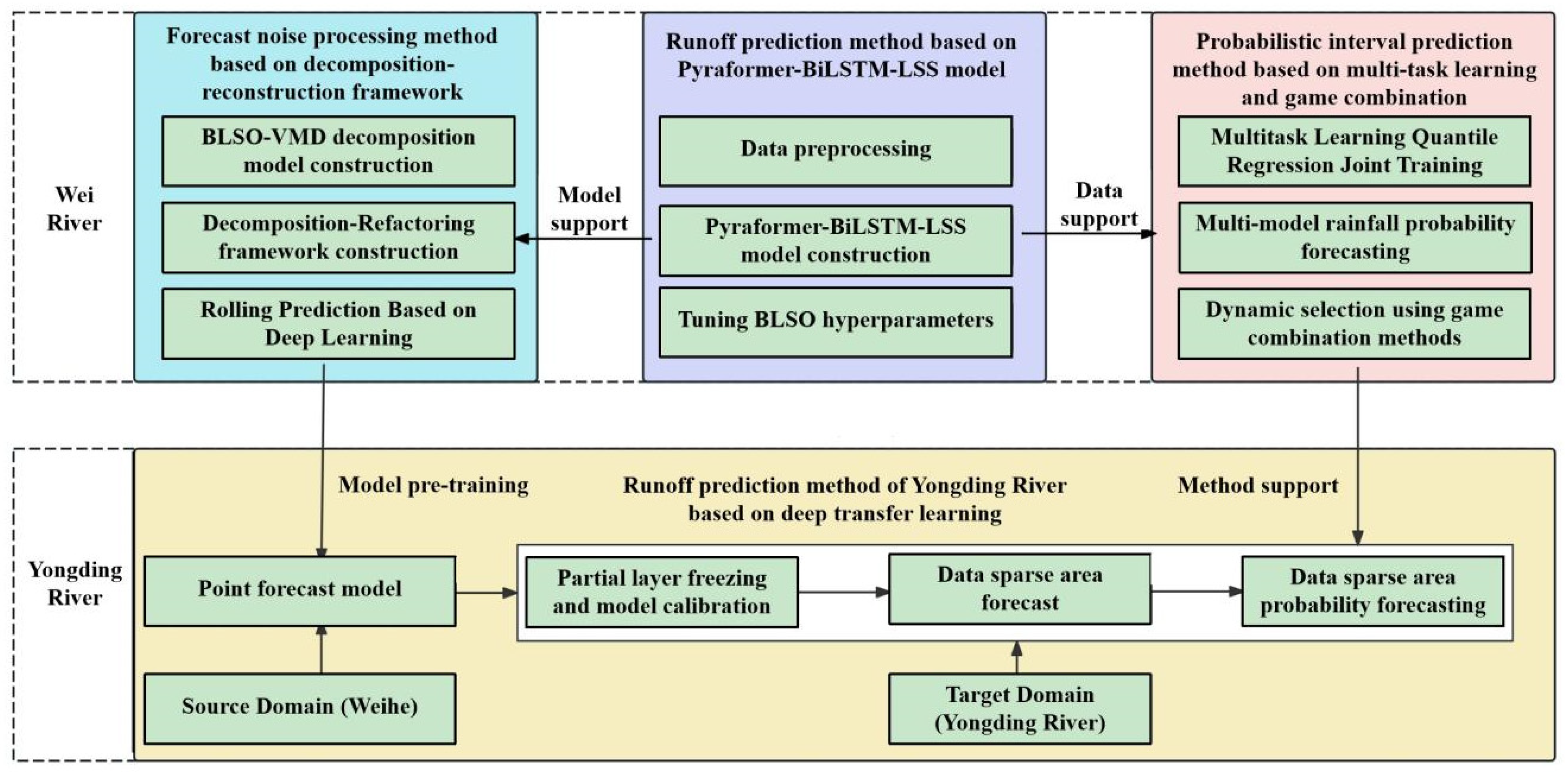
This study establishes a transfer-based runoff modeling framework with the Wei River as the source domain and the Yongding River as the target domain. By transferring model knowledge trained in the source domain to the target basin, it enables runoff forecasting in data-sparse regions. The model system comprises four key technical modules, each logically interconnected and exhibiting significant synergistic effects. First, the Wei River runoff process is modeled using the deep learning model Pyraformer-BiLSTM-LSS, yielding a point forecasting model with high accuracy and robustness (see Section 3.2). Second, an improved signal decomposition model BLSO-VMD is constructed. Combined with the deep learning model, a decomposition–reconstruction framework is established to process forecasting noise (see Section 3.3). Then, a probabilistic interval forecasting model based on multi-task learning is developed to characterize runoff forecast uncertainty within a multi-task framework, as detailed in Section 3.4. Finally, the aforementioned model techniques are coupled by freezing selected layers of the source domain pre-trained model and fine-tuning it for the Yongding River basin, enabling precise forecasting in data-sparse regions, as described in Section 3.5. The technical workflow of this study is illustrated in Figure 2.

Figure 2. Schematic diagram of the technical route of the study.

3.2. A Runoff Forecasting Method Based on the Pyraformer-BiLSTM Model

In this study, the model establishes a comprehensive time series forecasting framework by constructing the Pyraformer-BiLSTM model and incorporating the LSS function. This framework effectively captures both global and local temporal dependencies when processing time series data, thereby enhancing the accuracy and robustness of forecasts. The complete forecasting process comprises several key steps: feature selection, data processing, time series modeling, and runoff forecasting.

First, in the feature selection phase, a decision tree model identifies factors most relevant to the forecasting target. Considering meteorological and hydrological variables, this study selected precipitation, potential evapotranspiration, relative humidity, sunshine duration, daily mean temperature, daily maximum temperature, daily minimum temperature, wind speed, and ten-day lagged runoff data as influencing factors. The decision tree algorithm identified the ten most relevant factors, providing comprehensive input data for subsequent model training.

Second, a polynomial fitting method was employed to model the trend component within the time series. This effectively removed the trend component from the data, delivering cleaner input for subsequent time series modeling.

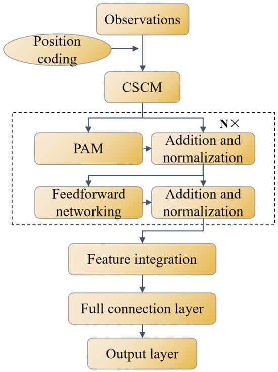
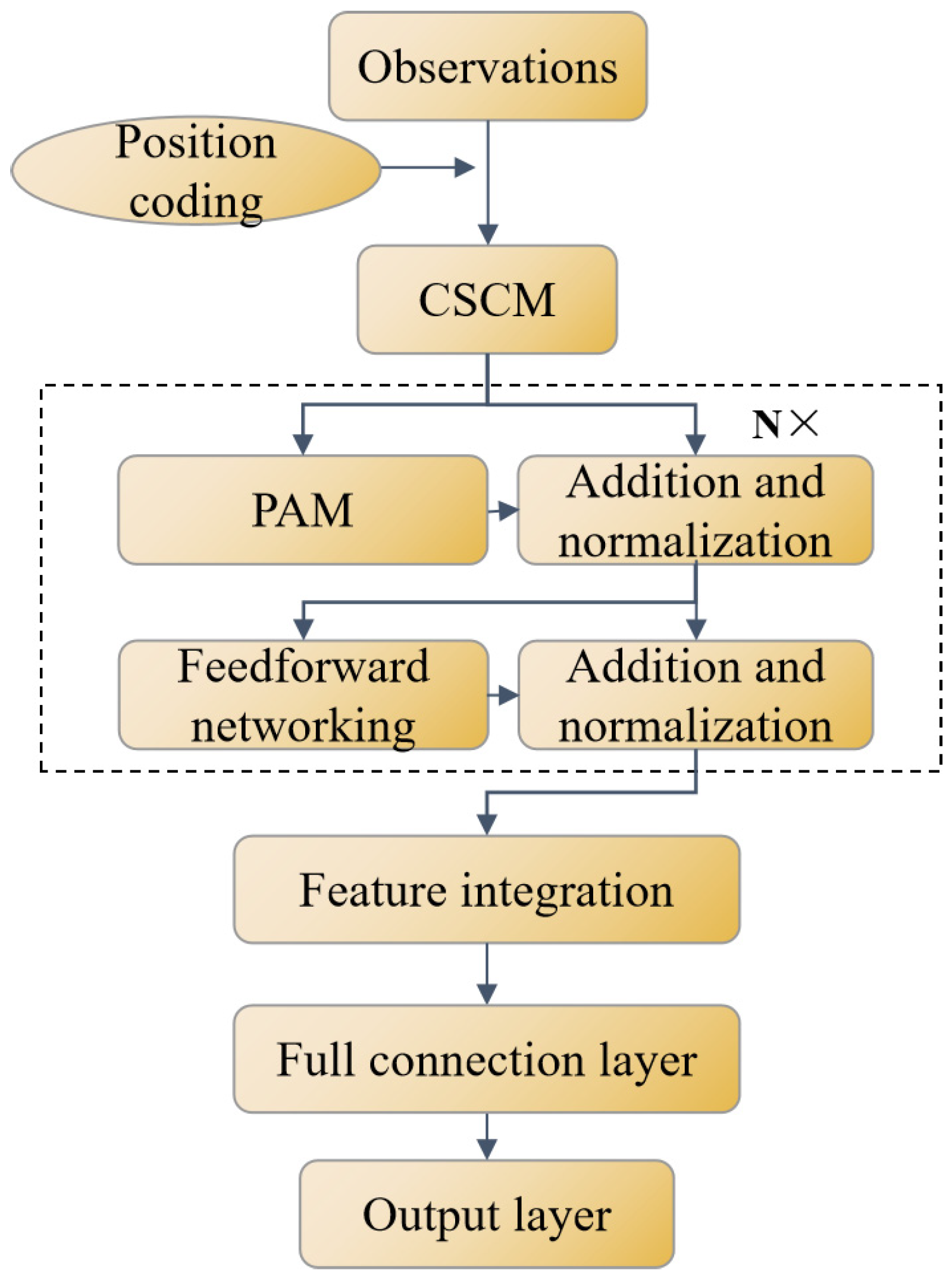
Next, as shown in Figure 3, the Pyraformer model is constructed. First, the input sequence undergoes embedding and positional encoding. Then, the Channel-Shifted Convolutional Module (CSCM) extracts local features at different scales. Immediately following this, the Pyramid Attention Module (PAM) is applied. Through addition and layer normalization steps, it captures both fine-grained and coarse-grained features. The sequence is then fed into a feedforward network. After each layer, summation and layer normalization steps are performed to maintain numerical stability and prevent gradient vanishing and exploding issues. Concurrently, adaptive residual connections dynamically adjust information flow between layers to stabilize training. Finally, a fully connected layer converts the extracted temporal features into prediction results through multi-layer mapping.

Figure 3. Flowchart of Pyraformer neural network structure.

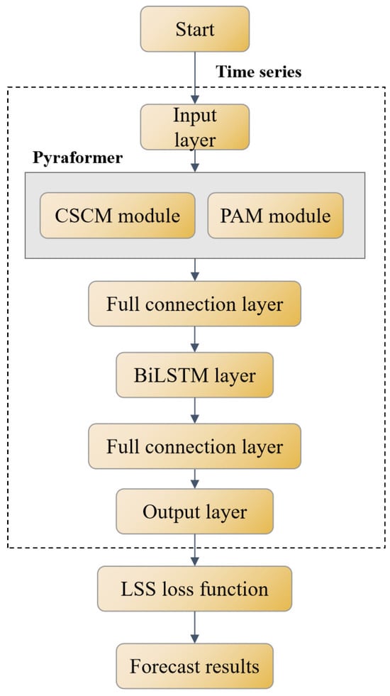
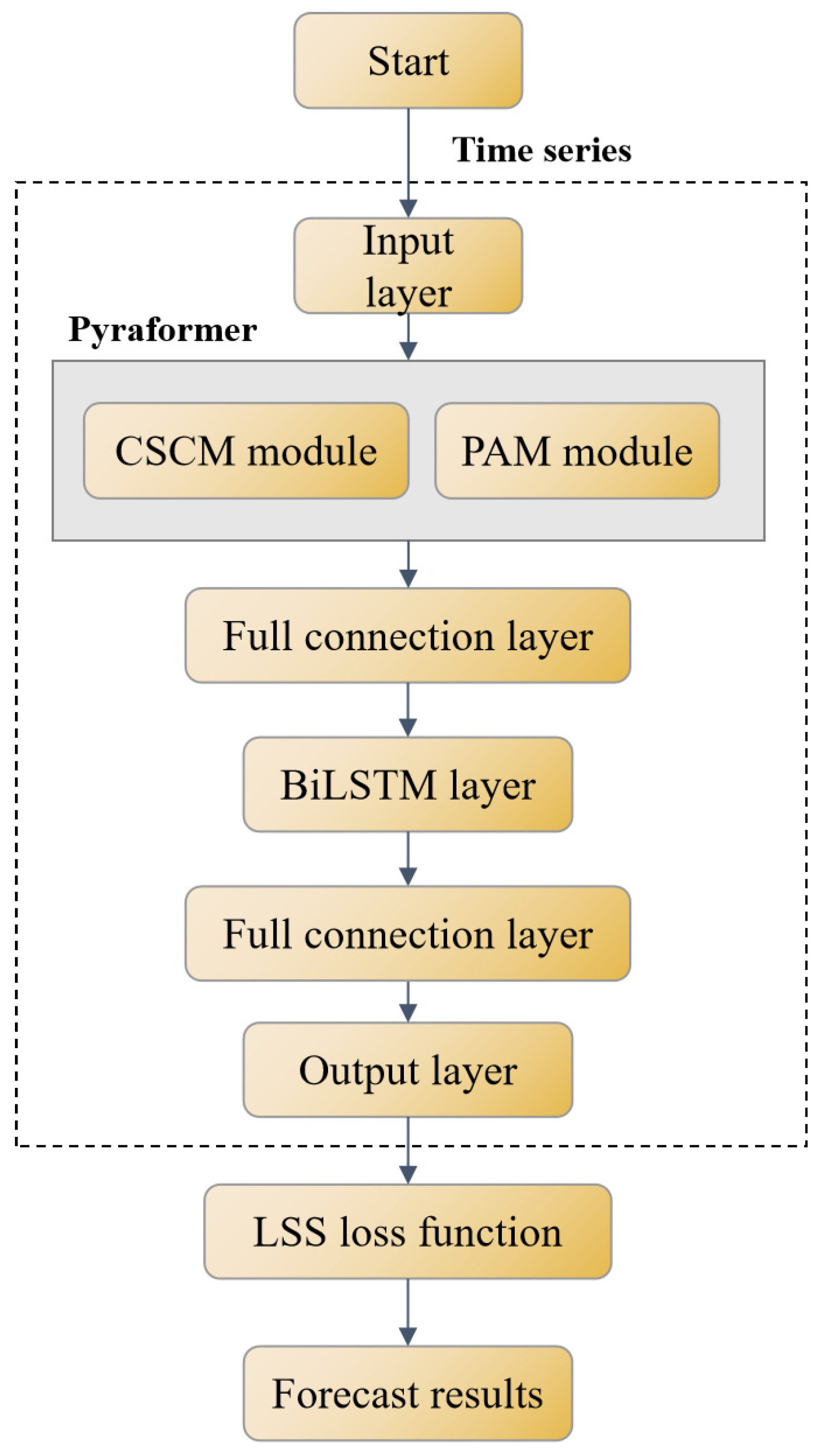
Subsequently, the Pyraformer-BiLSTM-LSS model is constructed, with its framework illustrated in Figure 4. This stage first employs Pyraformer for global temporal feature extraction. These global features are then passed through a fully connected layer to the BiLSTM layer. BiLSTM captures bidirectional dependencies in the sequence via forward and backward information flows, enabling the model to detect more complex and refined local temporal features within the time series. Subsequently, the model employs the Local Sensitivity to Sensitivity (LSS) [24] function to enhance sensitivity to local perturbations and outliers, thereby improving robustness against unstable runoff conditions and extreme scenarios.

Figure 4. Framework diagram of the Pyraformer-BiLSTM-LSS model.

Finally, the data is divided into training, validation, and test sets at an 8:1:1 ratio. Performance is evaluated using five metrics: Root Mean Square Error (RMSE), Mean Square Error (MSE), Mean Absolute Error (MAE), Mean Absolute Percentage Error (MAPE), and Coefficient of Determination (R-squared, R²). This empirical evaluation provides substantive support for the model’s effectiveness.

3.3. Forecast Noise Processing Method Based on a Decomposition–Reconstruction Framework

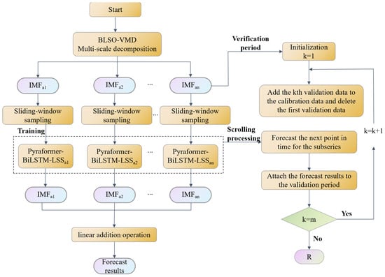
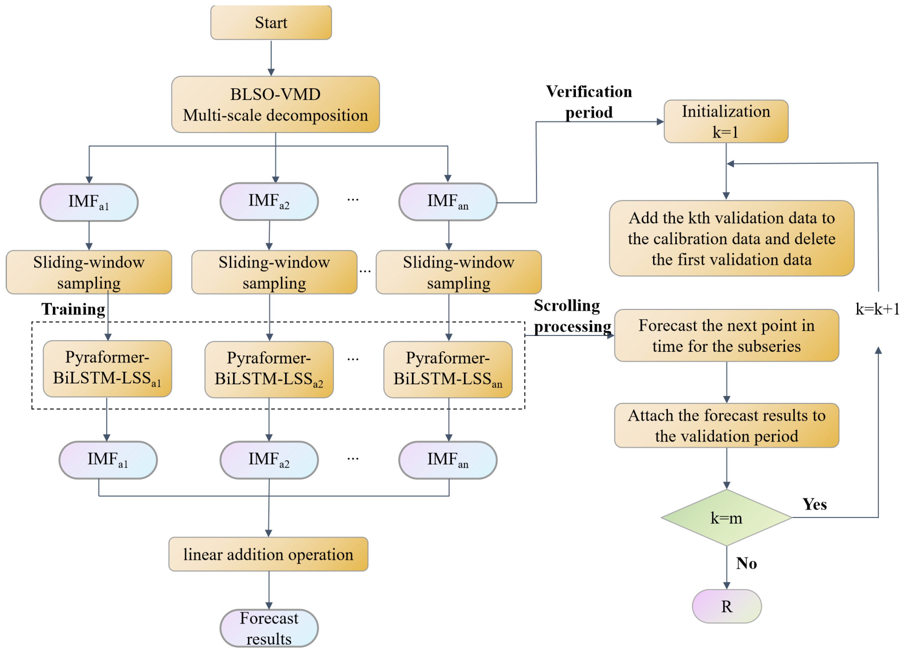
In the process of modeling runoff time series, the original sequence typically contains complex waveform structures, including trend, periodicity, seasonality, and high-frequency disturbances. These components directly impact the model’s ability to recognize data structures and forecast accuracy. To address this, this study constructs a rolling forecast framework based on decomposition–reconstruction. Its core lies in effectively decoupling signal decomposition from model forecasting, while employing a rolling mechanism to achieve dynamic training and continuous updates. This approach resolves data leakage issues during decomposition, collectively enhancing the model’s generalization capability and timely response performance in non-stationary environments. The framework flowchart is shown in Figure 5.

Figure 5. Flowchart of decomposition–reconstruction rolling forecast framework.

First, the BLSO-VMD model is employed to perform multimodal decomposition on the sequence. The Bloodsucking Leech Optimization (BLSO) [25] algorithm is introduced to adaptively optimize the number of modes (K) and the maximum iteration count in Variational Modal Decomposition (VMD). This process begins by initializing the parameter search space. The BLSO algorithm employs a global search strategy based on Bayesian inference, iteratively computing the objective function value to identify the optimal parameter configuration. Subsequently, the optimized VMD model processes the original runoff sequence, decomposing it into multiple intrinsic modal functions (IMFs) with distinct center frequencies and non-overlapping frequency domains.

Each IMF component is then treated as an independent training sample and input into the Pyraformer-BiLSTM-LSS model for modeling and forecasting. To mitigate forward information leakage in the decomposition–reconstruction framework, this study incorporates a rolling forecast mechanism. This strategy constructs fixed-length sliding time windows. During each training iteration, the model updates parameters using only historical data within the current window and predicts the next-time-step runoff based on the latest observation at the window’s trailing edge. As the forecast step advances, the time window dynamically shifts forward, discarding the oldest data and incorporating new observations for each update. Finally, the independent forecast results from each IMF component are linearly reconstructed to obtain the complete runoff forecast sequence.

All submodel forecasts are then aligned temporally and linearly combined to reconstruct the full forecast sequence, completing the end-to-end forecasting process from decomposition to reconstruction. The overall framework enhances feature separation through the BLSO-VMD decomposition method, improves multiscale sequence representation via Pyraformer-BiLSTM-LSS modeling, and ensures temporal consistency at the structural level through rolling mechanisms. This constitutes a forecasting scheme characterized by strong generalization, high accuracy, and robust stability.

3.4. Probabilistic Forecasting Model Based on Multi-Task Learning and Game Combination

To effectively quantify the uncertainty in runoff forecasting and establish reliable prediction intervals, this study proposes a quantile regression framework based on multi-task learning mechanisms. Using point forecasts as the baseline, this framework jointly trains multiple quantile tasks at different confidence levels to directly output upper and lower bounds for intervals corresponding to varying degrees of certainty. This approach probabilistically characterizes the range of future runoff variations.

First, the foundational quantile regression model is constructed. For a given dataset ${\left\{\left({\mathrm{x}}_{\mathrm{i}},{\mathrm{y}}_{\mathrm{i}}\right)\right\}}_{\mathrm{i}=1}^{\mathrm{n}}$, quantile regression estimates the conditional quantile function ${\mathrm{Q}}_{\mathrm{y}}\left(\tau \mid \mathrm{x}\right)$ by optimizing the asymmetric loss function ${\rho }_{\tau }\left(\mathrm{u}\right)=\mathrm{u}\left(\tau -\mathrm{I}\left(\mathrm{u}<0\right)\right)$, where the indicator function $\mathrm{I}\left(\mathrm{u}<0\right)$ imposes differential penalty weights on positive and negative deviations, enabling optimal fitting at the target quantile point τ. Within a deep learning framework, the Pyraformer-BiLSTM model serves as the architecture. Input sequences undergo multi-scale global feature extraction via the Pyraformer module, followed by bidirectional LSTM layers to capture temporal dependencies. The output layer configures multiple parallel fully connected heads, with each output node corresponding to the predicted value for a specific quantile τ, directly generating interval boundaries at confidence levels of 0.1, 0.5, and 0.9. The training process employs weighted quantile loss ${\mathrm{L}}_{\tau }\left(\theta \right)={\displaystyle {\sum }_{\mathrm{i}=1}^{\mathrm{n}}}{\rho }_{\tau }\left({\mathrm{y}}_{\mathrm{i}}-{\widehat{\mathrm{y}}}_{\mathrm{i}}\right)$ as the optimization objective, iteratively updating parameters via the Adam optimizer.

Second, a multi-task learning mechanism is introduced to enhance the model architecture. To avoid computational redundancy and interval inconsistencies caused by modeling each quantile point separately, this study unifies the prediction tasks for different confidence levels within a single network framework for parallel learning. Specifically, input data first undergoes feature extraction through a shared embedding layer and Pyraformer attention module, then passes through a bidirectional LSTM layer for temporal modeling. At the network’s end, dedicated output heads are configured for each target quantile Tm(m = 1, 2, …, M). These heads share preceding layer parameters while independently executing regression tasks, enabling the model to simultaneously output predictions for multiple quantiles in a single forward pass.

A multi-task joint training strategy is then designed. Loss functions for each quantile task are weighted and aggregated to form a unified optimization objective:

$${\mathrm{L}}_{\mathrm{m}}={\displaystyle {\sum }_{\mathrm{i}=1}^{\mathrm{N}}}\left[{\mathbb{I}}_{{\widehat{\mathrm{y}}}_{\mathrm{m}}}\left({\widehat{\mathrm{y}}}_{\mathrm{m}}\ge {\mathrm{y}}_{\mathrm{m}}\right)+{\mathbb{I}}_{{\mathrm{y}}_{\mathrm{m}}}\left({\mathrm{y}}_{\mathrm{m}}\ge {\widehat{\mathrm{y}}}_{\mathrm{m}}\right)\right]$$

(1)

$${\mathrm{L}}_{\mathrm{total}}={\displaystyle {\sum }_{\mathrm{m}=1}^{\mathrm{M}}}{\lambda }_{\mathrm{m}}{\mathrm{L}}_{\mathrm{m}}$$

(2)

In the equation, ${\lambda }_{\mathrm{m}}$ represents the weight coefficient for the mth task. Through this weighting mechanism, the model adaptively adjusts the optimization direction based on the importance of different confidence levels. During training, tasks at different quantiles exchange information through shared hidden layers. This preserves output independence while leveraging inter-task correlations to enhance overall learning efficiency. Ultimately, the model completes joint optimization for all quantiles within the same training cycle. The output layer sequentially provides predictions corresponding to each confidence level, directly constructing a probabilistic forecast interval with consistent structure.

Finally, a comprehensive evaluation metric system is established to quantify interval forecast performance. This framework evaluates performance across three dimensions: reliability, accuracy, and overall quality. It employs the Probability of Interval Coverage (PICP) to measure the interval’s ability to encompass observed values, utilizes the Probability of Interval Normalized Average Width (PINAW) to quantify interval compactness, and applies the Continuous Ranking Probability Score (CWC) to comprehensively balance coverage and interval width. Additionally, the Mean Prediction Interval Coverage Deviation (MPICD) is introduced to evaluate the consistency between actual coverage and target confidence level, while the Average Interval Score (AIS) comprehensively measures the joint penalty for interval width and coverage failure. This framework achieves a complete transition from point forecasts to probabilistic interval forecasts, providing a systematic technical pathway for quantifying uncertainty in runoff forecasting.

3.5. Deep Transfer Learning-Based Forecasting Model

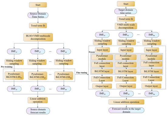
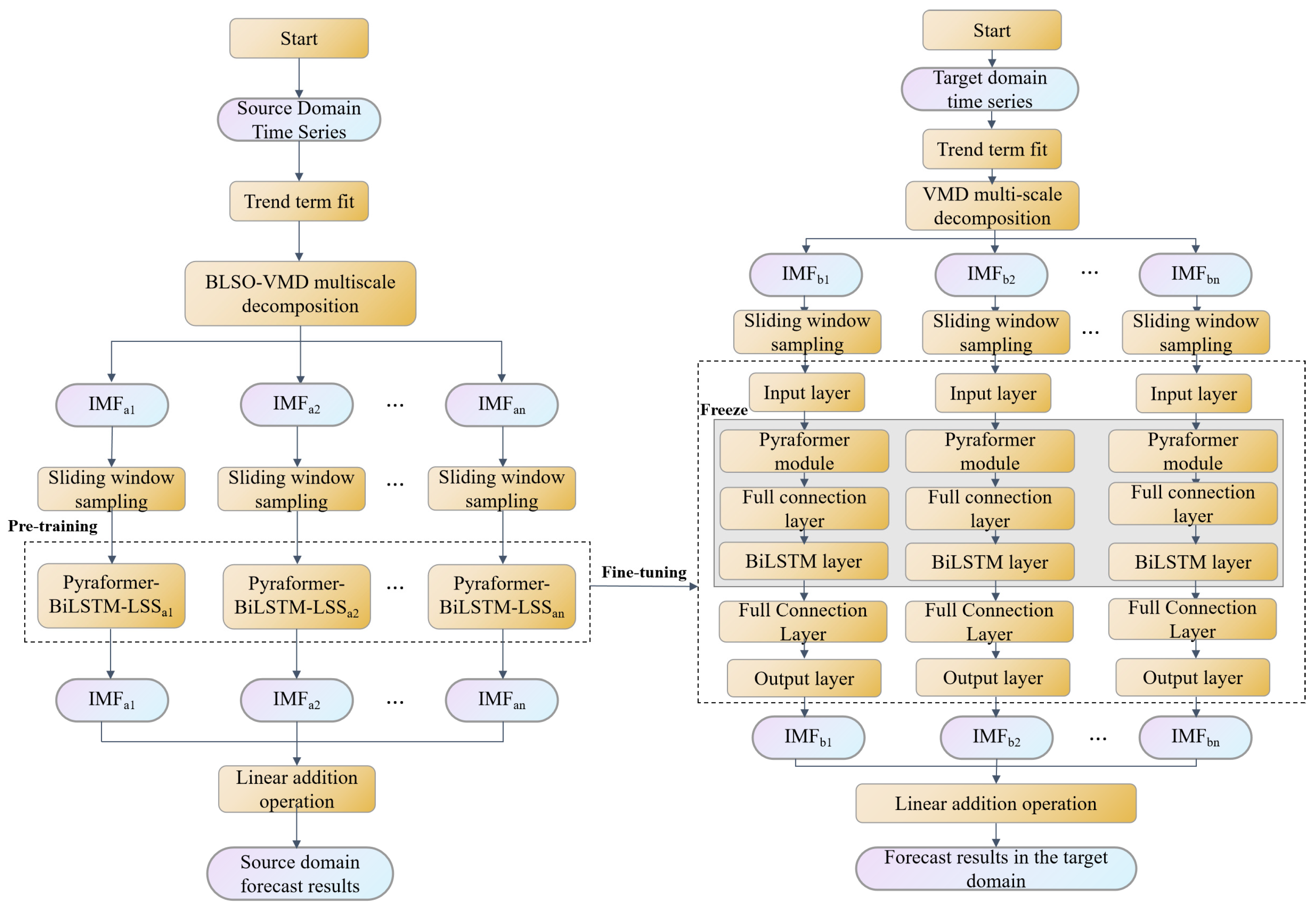
The model framework based on deep transfer learning proposed in this study aims to construct a forecasting model applicable to the target watershed using long-term historical data from the source watershed and short-term real-time data from the target watershed. The framework diagram is shown in Figure 6. This framework includes the following key steps:

Figure 6. Framework diagram of deep transfer learning.

Step 1: Trend component fitting for source domain time series. Extract the long-term trend component from the source domain time series and remove the trend component from the raw data.

Step 2: Source Basin Sequence Decomposition. The historical runoff time series from the source basin is decomposed into multiple Intrinsic Modal Functions (IMFs) using the BLSO-VMD method, revealing multi-level periodic characteristics within the sequence.

Step 3: Sliding time window sampling. Based on the time series data of each IMF component, data is sampled using a sliding time window method to construct a sample library. Data from each IMF component is divided into multiple time windows for subsequent model training. 80% of the data is allocated as the training set, 10% as the validation set, and the remaining 10% as the test set. The sliding time window ensures data participates in model training in a serialized manner.

Step 4: Forecasting using deep learning models. Train the Pyraformer-BiLSTM-LSS model on the data samples. The Pyraformer module extracts long-range dependency features, the BiLSTM layer captures bidirectional dependencies within the time series, and LSS enhances model robustness by measuring sensitivity. Forecast results are computed independently for each IMF component. After validation and testing, retain the forecast model that performs best on the test set.

Step 5: Obtain source domain forecast results. By linearly summing the forecast results for each IMF component, the final source domain runoff forecast values are obtained.

Due to challenges in collecting hydrological data for some basins and cross-sections, limited runoff data makes effective training and forecasting with deep learning models difficult. To meet practical engineering needs, we combine deep learning models, decomposable-ensemble frameworks, and transfer learning methods to transfer pre-trained models built for source basins. We freeze certain network layers and fine-tune only the fully connected layers and output layers based on target domain data. The specific steps are:

Step 6: Construct the transfer learning model. Establish a neural network framework identical to the source basin pre-trained model structure, fixing parameters of key layers including the positional embedding layer, self-attention layer, normalization layer, and BiLSTM layer.

Step 7: Target domain trend component fitting. Extract the long-term trend component from the target domain time series and remove the trend component from the raw data.

Step 8: Target domain decomposition and sliding time window sampling. Decompose target domain data using BLSO-VMD parameters consistent with the source domain to obtain multiple IMF components. Then, sample each IMF component via a sliding time window. The dataset partitioning method for constructing the sample library is 3:1:1.

Step 9: Model fine-tuning. Apply the source basin pre-trained model to the target basin, fine-tuning the fully connected layers and output layer within the target basin model. To prevent overfitting, the fine-tuning process is limited to 50 iterations with a learning rate set to 0.1 times that of the source basin model.

Step 10: Obtain target domain forecast results. The fine-tuned model is used to train and validate each IMF component for the target basin. After obtaining the forecast results for each IMF component, they are weighted and summed to derive the final runoff forecast value for the target basin.

Through the above steps, deep transfer learning technology effectively transfers the forecasting capability from the source basin to the target basin. This approach overcomes the challenge of insufficient data in the target basin while preserving the long-term spatiotemporal characteristics of the source basin model.

3.6. Indicator Evaluation System

In evaluating interval forecasting models, this paper employs five key evaluation metrics: Prediction Interval Coverage Probability (PICP), Prediction Interval Normalized Average Width (PINAW), Continuous Ranked Probability Score (CWC), Mean Prediction Interval Coverage Deviation (MPICD), and Average Interval Score (AIS) to comprehensively evaluate the performance of the interval forecast models.

$$\mathrm{P}\mathrm{I}\mathrm{C}\mathrm{P}={\displaystyle \frac{1}{\mathrm{N}}}{\displaystyle \sum _{\mathrm{t}=1}^{\mathrm{N}}}\mathbb{I}\left({\mathrm{y}}_{\mathrm{t}}\in \left[{\mathrm{L}}_{\mathrm{t}},{\mathrm{U}}_{\mathrm{t}}\right]\right)$$

(3)

In the equation, y_t is the observed value, L_t and U_t are the lower and upper bounds of the forecast interval, respectively, and I is an indicator function that takes the value 1 when the actual value lies within the interval, and 0 otherwise.

$$\mathrm{P}\mathrm{I}\mathrm{N}\mathrm{A}\mathrm{W}={\displaystyle \frac{1}{\mathrm{N}}}{\displaystyle \sum _{\mathrm{t}=1}^{\mathrm{N}}}{\displaystyle \frac{{\mathrm{U}}_{\mathrm{t}}-{\mathrm{L}}_{\mathrm{t}}}{{\widehat{\mathrm{y}}}_{\mathrm{t}}}}$$

(4)

$$\mathrm{C}\mathrm{W}\mathrm{C}={\displaystyle \frac{1}{\mathrm{N}}}{\displaystyle \sum _{\mathrm{t}=1}^{\mathrm{N}}}\left|\mathrm{F}\left({\mathrm{y}}_{\mathrm{t}}\right)-\mathbb{I}\left({\mathrm{y}}_{\mathrm{t}}\in \left[{\mathrm{L}}_{\mathrm{t}},{\mathrm{U}}_{\mathrm{t}}\right]\right)\right|$$

(5)

In the equation, F(y_t) is the cumulative distribution function, $\mathbb{I}\left({\mathrm{y}}_{\mathrm{t}}\in \left[{\mathrm{L}}_{\mathrm{t}},{\mathrm{U}}_{\mathrm{t}}\right]\right)$ is an indicator function that indicates whether an observation falls within the forecast interval.

$$\mathrm{M}\mathrm{P}\mathrm{I}\mathrm{C}\mathrm{D}={\displaystyle \frac{1}{\mathrm{N}}}{\displaystyle \sum _{\mathrm{t}=1}^{\mathrm{N}}}\left|{\displaystyle \frac{{\mathrm{C}}_{\mathrm{t}}-\mathrm{P}}{\mathrm{P}}}\right|$$

(6)

In the equation, C_t represents the actual coverage of the tth forecast, and P represents the target coverage. A smaller value indicates that the model’s forecast interval is more accurate.

$$\mathrm{A}\mathrm{I}\mathrm{S}={\displaystyle \frac{1}{\mathrm{N}}}{\displaystyle {\sum }_{\mathrm{t}=1}^{\mathrm{N}}}\left[\left({\mathrm{U}}_{\mathrm{t}}-{\mathrm{L}}_{\mathrm{t}}\right)+{\displaystyle \frac{2}{\mathrm{P}}}\left|\mathbb{I}\left({\mathrm{y}}_{\mathrm{t}}\in \left[{\mathrm{L}}_{\mathrm{t}},{\mathrm{U}}_{\mathrm{t}}\right]\right)-1\right|\right]$$

(7)

In the equation, P is the confidence level of the forecast interval. A smaller AIS value indicates a higher quality of the model’s forecast interval.

4. Results

4.1. Analysis of Point Runoff Forecast Results

This chapter systematically evaluates the proposed Pyraformer-BiLSTM-LSS model and its performance within the decomposition–reconstruction framework. Comparative experiments demonstrate (Table 1) that among standalone models, BiLSTM achieves an RMSE of 149.294 m³/s, outperforming both LSTM and GRU. Through model combination and optimization, Pyraformer-BiLSTM further reduces RMSE to 110.984 m³/s. The Pyraformer-BiLSTM-LSS model, constructed by incorporating the LSS loss function, achieved an RMSE of 114.093 m³/s. It demonstrated more balanced performance across metrics such as MAE and MAPE, exhibiting the best overall performance. This model maintained stable performance across different dataset partitions, particularly showing optimal generalization capability on the validation set (Table 2), confirming the effectiveness of its architecture.

Table 1. Results of model performance evaluation.

Type	Model	RMSE (m3/s)	MSE (m6/s2)	MAE (m3/s)	MAPE (%)	R2 (%)
Single forecast model	GRU	184.7	34,127.1	57.9	18.9	55.5
	LSTM	189.0	35,732.2	65.1	25.1	53.1
	BiLSTM	149.2	22,288.8	50.7	18.5	72.3
Conventional combinatorial model	Pyraformer-GRU	140.0	19,627.3	50.9	21.4	74.2
	Pyraformer-LSTM	124.1	15,415.3	42.1	15.1	79.7
	Pyraformer-BiLSTM	110.9	12,317.4	42.9	86.1	80.2
LSS-Combined model	Pyraformer-GRU-LSS	122.8	15,080.8	42.7	15.9	80.2
	Pyraformer-LSTM-LSS	119.3	14,236.3	194.0	16.7	81.3
	Pyraformer-BiLSTM-LSS	114.0	13,017.3	41.8	16.4	82.9

Table 2. Evaluation metrics for different dataset splits of pyraformer-BiLSTM-LSS.

Dataset Division	RMSE (m3/s)	MSE (m6/s2)	MAE (m3/s)	MAPE (%)	R2 (%)
Training set	101.9	10,394.2	35.1	96.3	83.3
Validation set	49.6	2469.3	23.7	23.0	86.7
Test set	114.0	13,017.3	41.8	16.4	82.9

In comparative experiments of decomposition–reconstruction frameworks (Table 3), the BLSO-VMD model demonstrated significant advantages, achieving an R² of 99.1% for its forecast results. All error metrics significantly outperformed the non-decomposed model and the BLSO-CEEMDAN model, validating this method’s capability to filter out noise while preserving effective wave information. Parameter analysis indicates (Table 4) that the BLSO-VMD model achieves optimal performance with 6 IMFs, demonstrating the critical role of the BLSO module in optimizing decomposition parameters and preventing over-decomposition. Furthermore, multi-step rolling forecast experiments (Table 5) reveal that although model accuracy decreases with increasing forecast lead time, it maintains an R² value of 92.3% at the 7-day forecast scale, demonstrating excellent temporal adaptability and forecast stability. In summary, the integration of the Pyraformer-BiLSTM-LSS model with the BLSO-VMD decomposition–reconstruction framework achieves both high accuracy and strong robustness when handling complex runoff sequences.

Table 3. Results of runoff forecasting under different decomposition models.

Section	Model	RMSE (m3/s)	MSE (m6/s2)	MAE (m3/s)	MAPE (%)	R2 (%)
Huaxian	BLSO-VMD	25.7	663.5	13.9	7.8	99.1
	BLSO-CEEMDAN	72.4	5248.9	28.5	1.2	93.1
	Does not decompose	114.0	13,017.3	41.8	16.4	82.9

Table 4. Results of runoff forecasting using the VMD model under different IMF numbers.

IMF	RMSE (m3/s)	MSE (m6/s2)	MAE (m3/s)	MAPE (%)	R2 (%)
3	49.2	2428.0	22.4	105	968
4	42.1	1780.4	19.7	9.3	97.6
5	30.3	921.3	14.2	6.9	98.7
6	25.7	663.5	13.9	7.8	99.1
7	25.9	664.1	14.1	7.9	99.1
8	26.4	697.5	11.5	6.1	99.0

Table 5. Results of runoff forecasting under different forecast scales.

Forecast Scale (Days)	RMSE (m3/s)	MSE (m6/s2)	MAE (m3/s)	MAPE (%)	R2 (%)
1	25.7	663.5	13.9	7.8	99.1
2	41.7	1746.3	18.1	8.1	97.7
3	53.4	2854.3	22.8	10.5	96.2
4	60.5	3668.3	25.2	11.1	95.1
5	67.8	4606.0	29.1	13.3	93.9
6	71.4	5111.7	30.4	13.5	93.2
7	76.2	5800.1	33.5	15.3	92.3

In summary, the BLSO-VMD model based on the decomposition–reconstruction framework demonstrated the best performance across all comparative experiments in runoff forecasting. Its superior fitting capability and low error levels make it an ideal choice for handling complex hydrological data, particularly in forecasting tasks involving highly fluctuating runoff. Furthermore, the model maintains high accuracy and stability as forecast lead times increase, demonstrating the robust performance of the Pyraformer-BiLSTM-LSS and BLSO-VMD combination for watershed runoff forecasting.

4.2. Analysis of Forecast Uncertainty Results

To validate the effectiveness of multi-task learning mechanisms in probabilistic interval forecasting, this section systematically compares the performance of different interval forecasting models with and without the multi-task learning framework, using the Wei River’s Huaxian section as a case study. The experiments selected BVMD-GRU, BVMD-LSTM, BVMD-BiLSTM, and their combined models with Pyraformer. Interval forecasts were conducted at three confidence levels (0.9, 0.6, and 0.3), and five evaluation metrics were used to quantitatively assess the models’ coverage capability, interval compactness, and overall reliability (Table 6, Table 7 and Table 8).

Table 6. Evaluation results of different interval forecasting models at 0.9 confidence level.

Interval Forecast Model		PICP (%)	PINAW (%)	CWC (%)	MPICD (m3/s)	AIS (m3/s)
Baseline model	BVMD-GRU	86.72	9.29	22.19	112.20	248.39
	BVMD-LSTM	85.78	8.75	22.09	115.39	269.43
	BVMD-BiLSTM	86.37	8.79	21.42	108.27	246.81
	BVMD-Pyraformer	94.24	16.88	16.88	171.21	231.20
	BVMD-Pyraformer-GRU	87.19	7.03	16.34	91.94	223.50
	BVMD-Pyraformer-LSTM	82.61	6.17	19.09	95.76	251.21
	BVMD-Pyraformer-BiLSTM	92.36	13.17	13.17	143.24	232.38
Multi-task learning model	Multitasking learning BVMD-GRU	88.72	7.88	16.83	89.69	194.07
	Multitasking learning BVMD-LSTM	80.85	6.43	22.50	97.62	251.56
	Multitasking learning BVMD-BiLSTM	88.48	7.93	17.16	90.39	194.98
	Multitasking learning BVMD-Pyraformer-GRU	88.72	7.79	16.63	92.00	210.64
	Multitasking learning BVMD-Pyraformer-LSTM	84.14	6.59	18.43	97.27	242.15
	Multitasking learning BVMD-Pyraformer-BiLSTM	92.48	6.35	13.16	38.98	37.47

Table 7. Evaluation results of different interval forecasting models at 0.6 confidence level.

Interval Forecast Model		PICP (%)	PINAW (%)	CWC (%)	MPICD (m3/s)	AIS (m3/s)
Baseline model	BVMD-GRU	59.34	2.80	5.79	100.48	366.22
	BVMD-LSTM	61.46	3.07	3.07	97.75	346.46
	BVMD-BiLSTM	61.69	3.70	3.70	93.76	320.64
	BVMD-Pyraformer	72.15	4.87	4.87	110.23	403.47
	BVMD-Pyraformer-GRU	64.75	3.98	3.98	93.40	318.30
	BVMD-Pyraformer-LSTM	64.28	3.91	3.91	92.79	318.17
	BVMD-Pyraformer-BiLSTM	66.74	4.72	4.72	88.19	294.91
Multi-task learning model	Multitasking learning BVMD-GRU	69.33	4.69	4.69	92.02	303.90
	Multitasking learning BVMD-LSTM	68.39	3.87	3.87	98.64	347.04
	Multitasking learning BVMD-BiLSTM	68.04	4.72	4.72	93.04	306.67
	Multitasking learning BVMD-Pyraformer-GRU	67.10	4.25	4.25	94.42	319.56
	Multitasking learning BVMD-Pyraformer-LSTM	65.92	3.89	3.89	97.51	337.63
	Multitasking learning BVMD-Pyraformer-BiLSTM	72.74	3.92	3.92	99.82	330.65

Table 8. Evaluation results of different interval forecasting models at 0.3 confidence level.

Interval Forecast Model		PICP (%)	PINAW (%)	CWC (%)	MPICD (m3/s)	AIS (m3/s)
Baseline model	BVMD-GRU	33.84	1.74	1.74	97.37	378.42
	BVMD-LSTM	31.37	1.78	1.78	100.31	388.95
	BVMD-BiLSTM	35.84	2.16	2.16	93.53	361.48
	BVMD-Pyraformer	46.89	1.96	1.96	117.13	462.90
	BVMD-Pyraformer-GRU	37.37	1.71	1.71	93.32	363.95
	BVMD-Pyraformer-LSTM	37.13	1.57	1.57	95.11	374.08
	BVMD-Pyraformer-BiLSTM	41.83	2.47	2.47	88.76	345.19
Multi-task learning model	Multitasking learning BVMD-GRU	36.43	2.32	2.32	94.85	363.28
	Multitasking learning BVMD-LSTM	36.08	1.74	1.74	101.84	394.42
	Multitasking learning BVMD-BiLSTM	35.49	2.32	2.32	95.69	366.58
	Multitasking learning BVMD-Pyraformer-GRU	41.25	2.26	2.26	94.68	364.12
	Multitasking learning BVMD-Pyraformer-LSTM	44.42	2.21	2.21	96.11	374.88
	Multitasking learning BVMD-Pyraformer-BiLSTM	48.88	2.12	2.12	117.23	464.54

Regarding interval coverage capability, models employing multi-task learning generally demonstrated higher coverage rates, particularly at higher confidence levels. For instance, the multi-task learning BVMD-GRU achieved a PICP of 88.72% at the 0.9 confidence level, significantly outperforming the non-multi-task learning BVMD-GRU. BVMD-BiLSTM and BVMD-Pyraformer-BiLSTM also showed substantial improvements in PICP after incorporating multi-task learning mechanisms. This indicates that multi-task learning effectively enhances the model’s coverage of true values.

However, multi-task learning models typically exhibit wider interval widths. Although their interval coverage improves, the models’ interval width increases to maintain high PICP. For instance, the PINAW of the multi-task learning BVMD-GRU is 7.88%, slightly higher than the 9.29% of the non-multi-task learning model. This increase in interval width indicates that some multi-task learning models sacrifice accuracy to improve coverage.

Regarding interval stability, models employing multi-task learning generally reduce the error in forecast intervals. At a 0.9 confidence level, the CWC of the multi-task learning BVMD-GRU is 16.83%, lower than the 22.19% of the non-multi-task learning model, indicating that multi-task learning can enhance forecast stability to some extent.

From the perspective of comprehensive evaluation metrics, MPICD and AIS metrics also show certain advantages after applying multi-task learning. The MPICD of the multi-task learning BVMD-GRU model is 89.69%, smaller than the 112.20% of the non-multi-task learning BVMD-GRU model, indicating lower forecast errors and greater precision. Although the multi-task learning model’s AIS value is slightly higher, its adaptability remains strong, maintaining good stability and reliability.

In summary, models employing multi-task learning consistently outperform non-multi-task learning models across multiple key metrics, demonstrating particularly strong advantages in improving interval coverage and reducing forecast errors. Multi-task learning not only enhances the efficiency of probabilistic forecasting but also strengthens the model’s overall forecasting capability and robustness.

4.3. Analysis of Transfer Learning Forecast Results

To validate the effectiveness of the deep transfer learning framework in forecasting runoff in data-scarce basins, this section systematically compares the forecasting performance of models with and without transfer learning strategies, using the Guanting section of the Yongding River as a representative case study.

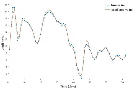
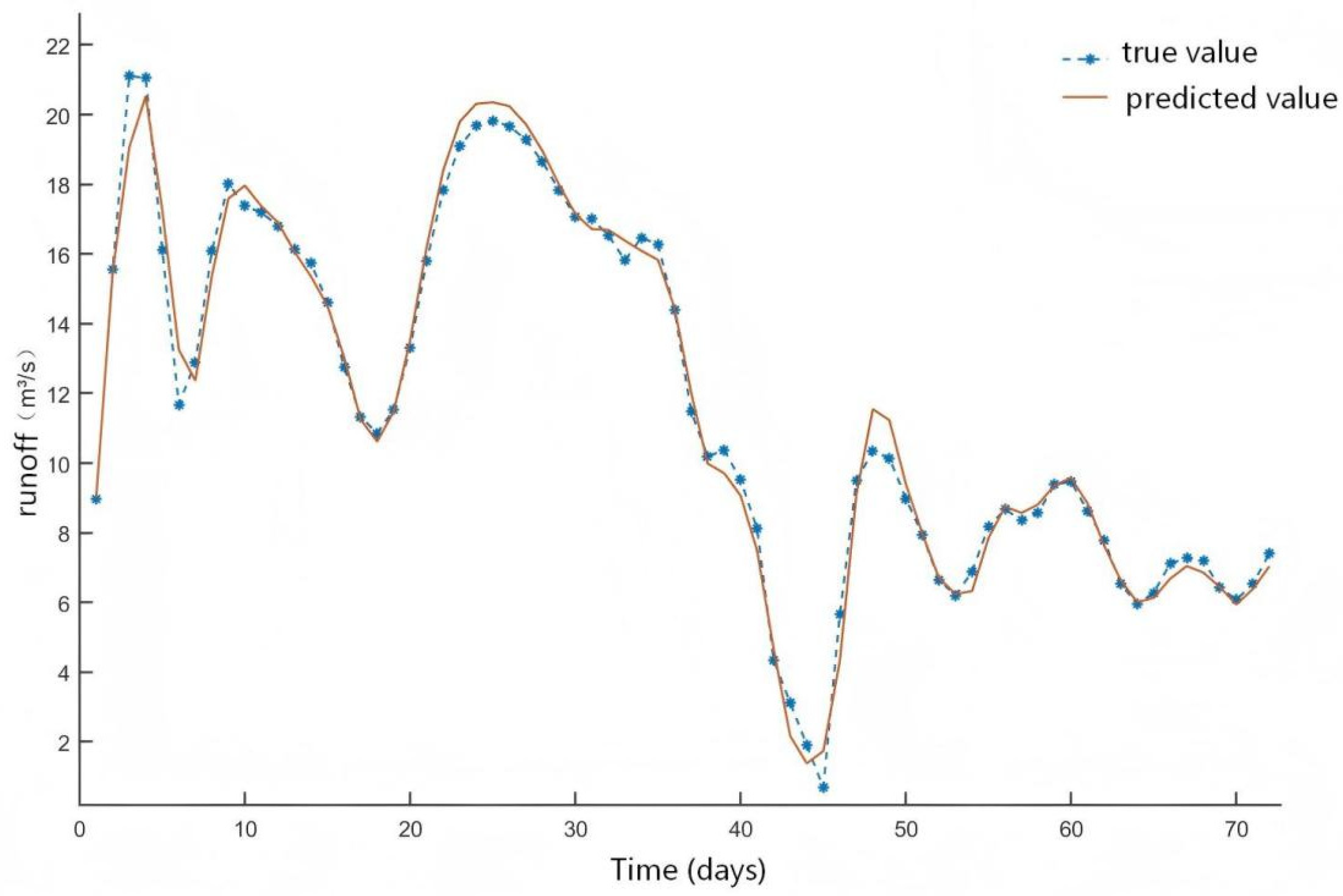
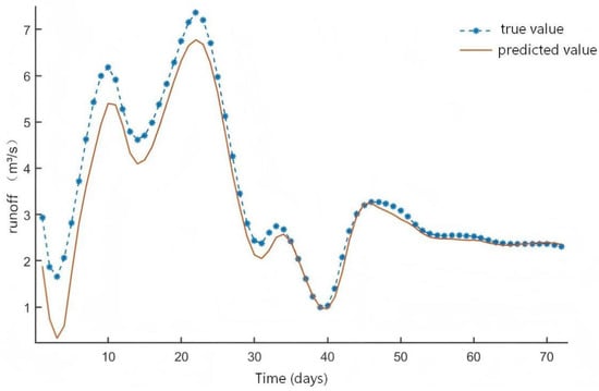
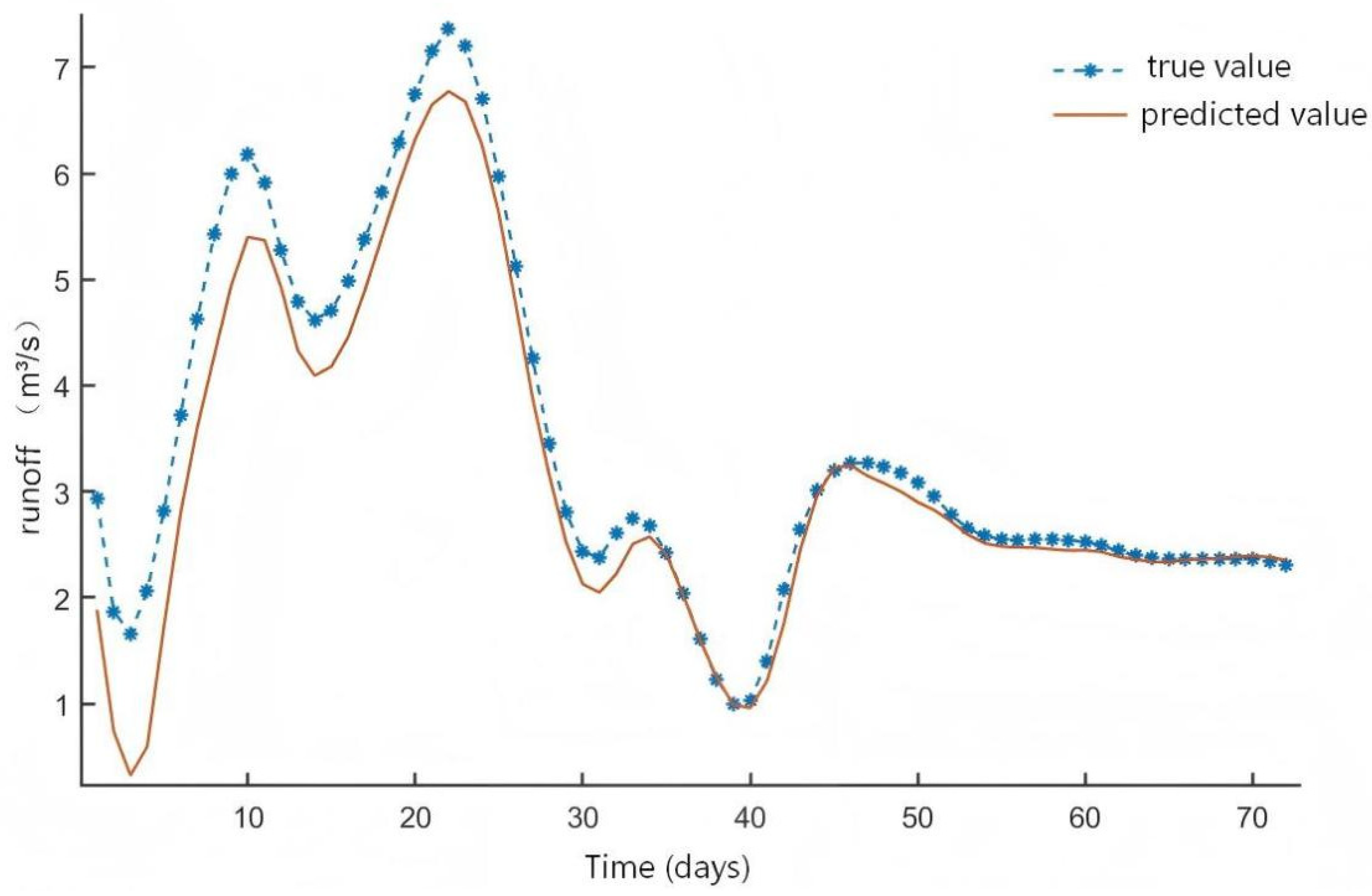
Table 9 presents the evaluation metrics for each dataset with and without transfer learning, while Figure 7 displays the forecast results under transfer learning. Compared to models without transfer learning, the transfer learning models demonstrate significantly improved performance on the test set. As shown in Table 9, the conventional forecasting model achieves acceptable results on the training set but performs notably poorly on the test set, with an R² of only 61.86% under data-scarce conditions. This indicates that models without transfer learning struggle to achieve effective forecasting and generalization under insufficient data. In contrast, models that utilize transfer learning demonstrated improved performance across all datasets, with a 57% increase in relative accuracy and a 35.55 percentage point increase in absolute accuracy on the test set. The visualization in Figure 7 further highlights the stability and robustness of these transfer learning-based forecasts.

Table 9. Evaluation metrics for dataset splits with and without the use of transfer learning.

Model	Dataset Division	RMSE (m3/s)	MSE (m6/s2)	MAE (m3/s)	MAPE (%)	R2 (%)
Deep learning models	Training set	0.69	0.49	0.57	16.16	95.04
	Validation set	1.35	1.81	0.89	15.97	86.47
	Test set	3.13	9.82	2.44	19.60	61.86
Deep transfer learning models	Training set	0.48	0.23	0.35	18.13	99.45
	Validation set	0.45	0.20	0.34	13.54	98.44
	Test set	0.81	0.66	0.59	7.85	97.41

Figure 7. Forecasting results for Guanting under transfer learning.

Based on point forecast results under transfer learning, further interval forecasts were conducted for the runoff at the Guanting section of the Yongding River. Table 10, Table 11 and Table 12 present the evaluation results of different interval forecasting models under varying confidence levels.

Table 10. Evaluation results of different interval forecasting models under transfer learning at the 0.9 confidence level.

Interval Forecast Model	PICP (%)	PINAW (%)	CWC (%)	MPICD (m3/s)	AIS (m3/s)
BVMD-Gaussian	54.17	5.02	185.64	0.6	1.2
BVMD-Bootstrap	68.06	6.88	68.59	0.6	0.98
BVMD-RF	93.06	95.98	95.98	4.18	4.66
multi-task learning BVMD-GRU	41.67	43.43	5498.8	6.91	15.26
multi-task learning BVMD-LSTM	11.11	27.04	72,157	8.46	24.3
multi-task learning BVMD-BiLSTM	43.06	44.28	4886.1	6.87	15
multi-task learning BVMD-Pyraformer-GRU	1.39	10.61	74,839.00	9.31	33.36
multi-task learning BVMD-Pyraformer-LSTM	4.17	13.57	72,526	9.8	34.31
multi-task learning BVMD-Pyraformer-BiLSTM	93.06	102.79	102.79	4.66	5.27

Table 11. Evaluation results of different interval forecasting models under transfer learning at the 0.6 confidence level.

Interval Forecast Model	PICP (%)	PINAW (%)	CWC (%)	MPICD (m3/s)	AIS (m3/s)
BVMD-Gaussian	34.72	2.57	34.73	0.6	1.95
BVMD-Bootstrap	38.89	2.83	26.22	0.6	1.94
BVMD-RF	51.39	49.37	166.16	5.45	16.12
multi-task learning BVMD-GRU	34.72	31.57	426.99	6.29	19.99
multi-task learning BVMD-LSTM	6.94	16.38	3315.4	7.63	26.68
multi-task learning BVMD-BiLSTM	36.11	32.24	383.7	6.25	19.76
multi-task learning BVMD-Pyraformer-GRU	1.39	6.37	2242.60	8.95	34.28
multi-task learning BVMD-Pyraformer-LSTM	1.39	5.28	1858.5	9.18	35.43
multi-task learning BVMD-Pyraformer-BiLSTM	61.11	52.7	52.7	4.89	14.33

Table 12. Evaluation results of different interval forecasting models under transfer learning at the 0.3 confidence level.

Interval Forecast Model	PICP (%)	PINAW (%)	CWC (%)	MPICD (m3/s)	AIS (m3/s)
BVMD-Gaussian	18.06	1.18	5.06	0.6	2.29
BVMD-Bootstrap	22.22	1.53	4.87	0.6	2.28
BVMD-RF	23.61	20.8	60.21	6.18	23.19
multi-task learning BVMD-GRU	26.39	15.64	38.08	5.75	22.01
multi-task learning BVMD-LSTM	1.39	5.8	107.21	6.87	26.78
multi-task learning BVMD-BiLSTM	26.39	15.86	38.62	5.71	21.89
multi-task learning BVMD-Pyraformer-GRU	0.00	0.19	3.96	7.91	31.63
multi-task learning BVMD-Pyraformer-LSTM	1.39	3.39	62.58	8.84	34.95
multi-task learning BVMD-Pyraformer-BiLSTM	31.94	22.17	22.17	5.33	20.4

In terms of overall forecasting performance, unlike the Huaxian section of the Wei River, the BVMD-Bootstrap model demonstrated the highest accuracy and reliability at all confidence levels for the Guanting section. As shown in the charts, this model effectively captures data trends with high interval coverage while achieving a balanced performance across other metrics.

As confidence levels decrease, the forecast interval widths of all models expand to varying degrees. Compared to the optimal model BVMD-Pyraformer-BiLSTM from the multi-task learning-based quantile regression model, both exhibit similar metrics and scores. However, the BVMD-Bootstrap model features a more compact forecast interval and effectively captures fluctuations in actual values. This robustness indicates the model’s ability to deliver stable forecasts even under high uncertainty. It suggests that in runoff interval forecasting tasks with limited data, deep learning models may underperform compared to simpler, effective models due to overfitting or learning excessive noise.

The interval forecasting model selection results for the Yongding River basin, while sharing similarities with the Wei River basin, exhibit distinct characteristics. Through the comprehensive evaluation method proposed in Section 4, optimal models can ultimately be dynamically selected across different river basins.

4.4. Runoff Forecast Results for Different Cross-Sections

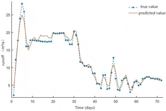
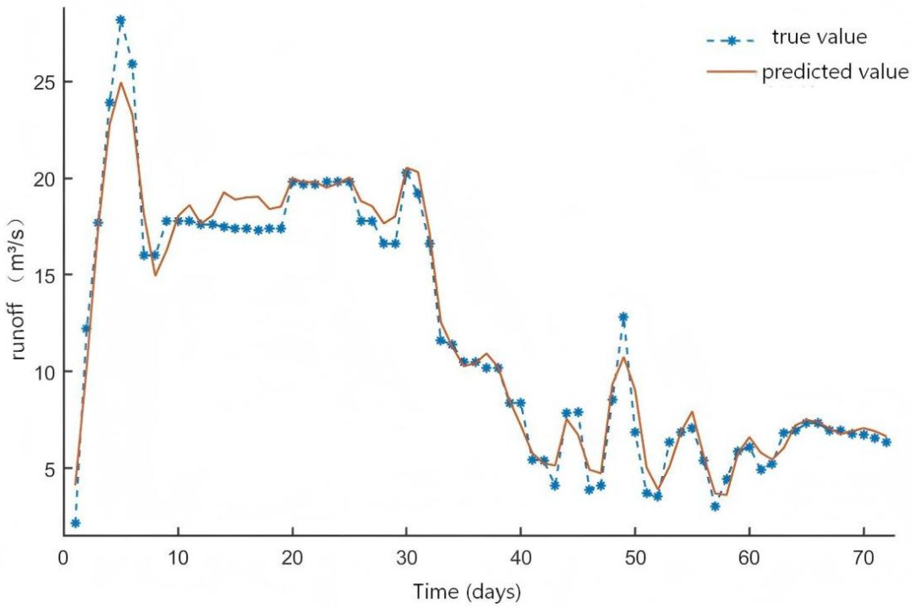
Through experimentation, the model’s effectiveness has been preliminarily validated. This section continues to verify the applicability of the proposed deep transfer learning model by testing it across different key cross-sections within the target watershed. Table 13 presents the forecast evaluation metrics for the Shixiali and Xiangshuipu cross-sections in the Yongding River basin, while Figure 8 and Figure 9 visualize the forecast results respectively.

Table 13. Evaluation metrics for runoff forecasting at different sections under transfer learning.

Section	Dataset Division	RMSE (m3/s)	MSE (m6/s2)	MAE (m3/s)	MAPE (%)	R2 (%)
Shixiali	Training set	0.42	0.17	29.57	8.32	99.56
	Validation set	0.50	0.25	34.94	16.06	73.73
	Test set	1.05	1.10	78.38	8.97	97.29
Xiangshuipu	Training set	0.16	0.02	9.73	9.77	99.36
	Validation set	0.71	0.51	53.27	8.36	93.17
	Test set	0.48	0.23	32.66	9.89	91.08

Figure 8. Forecasting results for Shixiali under transfer learning.

Figure 9. Forecasting results for Xiangshuipu under transfer learning.

At both the Shixiali and Xiangshuipu cross-sections, the model demonstrated high accuracy across the training, validation, and test datasets, achieving R² values of 97.29% and 91.08% on the test set, respectively. These metrics indicate that the constructed model can deliver stable forecasts across different cross-sections, maintaining robust predictive performance through transfer learning even under data-scarce conditions. Figure 8 and Figure 9 reveal excellent fitting quality with minimal fluctuations and negligible time lags, validating the model’s effectiveness and stability.

In summary, the proposed deep transfer learning model demonstrates broad applicability and significant potential for deployment across multiple cross-sections and river basins.

5. Discussion

5.1. Scientific Rationale and Significance of the Research Framework

This study addresses the challenge of runoff forecasting in hydrologically data-scarce basins by establishing a transfer learning modeling framework that bridges data-rich source basins (Wei River) to data-sparse target basins (Yongding River). The framework systematically integrates four key technological components: First, a Pyraformer-BiLSTM-LSS deep learning model is employed to establish a foundation for high-precision point forecasting; Second, an enhanced BLSO-VMD decomposition–reconstruction framework is applied to mitigate forecast noise and enhance stability. Third, a multi-task learning strategy generates probability intervals to quantify uncertainty. Finally, a “decomposition–reconstruction–transfer” strategy achieves cross-basin knowledge adaptation. This integrated technology establishes a comprehensive deep transfer learning approach that covers the entire process, from deterministic prediction, error correction, and uncertainty quantification to regional data transmission.

The core significance of this framework lies in providing a reusable technical paradigm for addressing the long-standing challenge of forecasting in data-poor/data-scarce regions within hydrology. By integrating universal hydrological patterns extracted through deep learning with targeted transfer calibration, this framework significantly reduces dependence on target basin data while ensuring forecast accuracy and reliability. This not only advances the frontier of hydrological forecasting methods but also provides a practical analytical tool for enhancing risk management capabilities in water-vulnerable regions, holding significant scientific value and application potential.

5.2. The Importance of Pyraformer-BiLSTM-LSS

Within the decomposition–reconstruction framework, this study developed the Pyraformer-BiLSTM-LSS deep learning forecasting model and the BLSO-VMD signal decomposition model based on the water-absorbing leech optimization algorithm. Together, they form a comprehensive runoff forecasting methodology. The Pyraformer-BiLSTM-LSS model integrates Pyraformer’s multi-scale dependency capture capability with BiLSTM’s bidirectional temporal feature extraction advantage, and incorporates the LSS mechanism to enhance model stability, thereby achieving higher accuracy and robustness in point forecasting under complex conditions such as non-stationarity and lag in runoff sequences. The BLSO-VMD model employs an optimization algorithm to adaptively determine decomposition parameters, effectively suppressing information leakage and endpoint effects prone in traditional VMD methods, thus ensuring signal decomposition accuracy and completeness. The combination fully leverages deep learning’s potential in feature extraction and forecasting modeling, alongside the optimization decomposition’s advantages in error separation and information refinement, collectively forming an efficient and reliable runoff forecasting system. By introducing a combined “decomposition + transfer learning” modeling approach, this framework fills a gap in the Yongding River Basin’s hydrological forecasting. Empirical results demonstrate that it achieves significantly higher forecasting accuracy than models relying solely on transfer learning or signal decomposition, thereby validating the effectiveness of this new method in improving forecasting performance in data-scarce basins.

5.3. Limitations

This study establishes a systematic framework for runoff forecasting in terms of deep learning modeling, signal decomposition, and transfer mechanisms, and validates it through experiments. However, due to time and computational resource constraints, several unresolved issues remain in the research process and require further investigation: (1) Future research could further enhance the model’s cross-basin generalization capability by exploring transfer learning mechanisms based on the fusion of multi-source basin information and incorporating meta-learning methods to achieve rapid adaptation and improved generalization accuracy for runoff forecasting in unknown regions. (2) Modeling strategies for integrating multi-source heterogeneous data could be further explored. By integrating remote sensing imagery, weather forecasts, and land surface characteristics to expand the range of input data, the model’s ability to capture changes in the watershed environment and extreme hydrological events is enhanced. (3) The model training and validation data in this study are current as of 2020, primarily due to the delayed release cycles of publicly available hydrological data and limitations in the quality of early-stage observations; the model’s performance under conditions of intensified extreme hydrological events after 2021 will require further validation once updated data become available.

6. Conclusions

This study addresses the challenges of nonlinearity, non-stationarity, and uncertainty quantification in runoff forecasting for data-scarce basins by proposing a collaborative modeling framework integrating point forecasting, interval forecasting, and transfer learning. Key findings are as follows: (1) The Pyraformer-BiLSTM-LSS hybrid deep learning model was developed to effectively extract multi-scale runoff features and enhance deterministic forecast accuracy. (2) The BLSO-VMD optimization decomposition technique was introduced to filter and reconstruct forecast noise, enhancing model robustness; (3) A probabilistic interval forecasting model was constructed using a multi-task learning strategy, achieving stable quantification of uncertainty. (4) Based on transfer learning mechanisms, the model knowledge trained on the Wei River basin was adapted to data-scarce basins like the Yongding River, significantly improving forecasting performance. Empirical results demonstrate that this framework achieves high accuracy across multiple cross-sections, effectively addressing critical challenges in runoff simulation for data-scarce regions—including noise interference, interval stability, and data insufficiency. It provides a systematic solution for reliable hydrological forecasting in areas with no or limited data.

References

- Wang, H.; Jia, Y. The Evolving Theory and Research Methods of the “Nature-Society” Dual Water Cycle in Watersheds. Acta Hydraul. Sin. 2016, 47, 1219–1226. [Google Scholar]
- Lu, Q. Research on the Current Status of Wetland Ecological Conservation and Sustainable Resource Management Models. Contemp. Agric. Mach. 2025, 72–73+75. (In Chinese) [Google Scholar]
- Chen, X.; Li, Q.; Jia, Z.; Xiao, R.; Cheng, Z.; Peng, Y. Study on the evolution of ecological flow in river and its guarantee degree during different hydrological periods. J. Clean. Prod. 2025, 490, 144761. [Google Scholar] [CrossRef] [Scilit]
- Bhattacharya, B.; Mazzoleni, M.; Chandra, M.L. Uncertainty Assessment of Hydrological Models of Large Basins with Limited Data—Experiences with the Brahmaputra Basin. In Proceedings of the 38th IAHR World Congress, Panama City, Panama, 1–6 September 2019; pp. 5879–5885. [Google Scholar]
- Li, Q.; Li, M.; Li, Z.; Huang, P.; Zheng, A. Analysis of the Physical Significance and Application of Parameters in the Xin’anjiang-Haihe River Model. J. Hohai Univ. (Nat. Sci. Ed.) 2025, 53, 1–9. [Google Scholar]
- Kiran, S.G.; Kumar, S.R.; Athira, P.; Reed, S. Modified calibration strategies and parameter regionalization potential for streamflow estimation using a hydrological model. Hydrol. Sci. J. 2024, 69, 765–781. [Google Scholar] [CrossRef] [Scilit]
- Chlumecky, M. Simulation of Hydrological Processes by Optimization Algorithm Using Continuous Function. In Proceedings of the 2015 Federated Conference on Software Development and Object Technologies; Janech, J., Kostolny, J., Gratkowski, T., Eds.; Springer International Publishing: Cham, Switzerland, 2017; Volume 511, pp. 110–121. [Google Scholar] [CrossRef] [Scilit]
- Nabi, K.N.; Tahmid, M.T.; Rafi, A.; Kader, M.E.; Haider, M.A. Forecasting COVID-19 cases: A comparative analysis between recurrent and convolutional neural networks. Results Phys. 2021, 24, 104137. [Google Scholar] [CrossRef] [Scilit]
- Song, H.; Choi, H. Forecasting Stock Market Indices Using the Recurrent Neural Network Based Hybrid Models: CNN-LSTM, GRU-CNN, and Ensemble Models. Appl. Sci. 2023, 13, 4644. [Google Scholar] [CrossRef] [Scilit]
- Deng, H.; Chen, W.; Huang, G. Deep insight into daily runoff forecasting based on a CNN-LSTM model. Nat. Hazards 2022, 113, 1675–1696. [Google Scholar] [CrossRef] [Scilit]
- Arsenault, R.; Martel, J.-L.; Brunet, F.; Brissette, F.; Mai, J. Continuous streamflow prediction in ungauged basins: Long short-term memory neural networks clearly outperform traditional hydrological models. Hydrol. Earth Syst. Sci. 2023, 27, 139–157. [Google Scholar] [CrossRef] [Scilit]
- Wellens, A.P.; Udenio, M.; Boute, R.N. Transfer learning for hierarchical forecasting: Reducing computational efforts of M5 winning methods. Int. J. Forecast. 2021, 38, 1482–1491. [Google Scholar] [CrossRef] [Scilit]
- Yin, S.; Xu, W.; Xiong, Y.; Tian, Y.; Zhao, S.; Chen, S. A Long Short-Term Memory Neural Network Hydrological Model Based on Transfer Learning. J. Hydropower Eng. 2022, 41, 53–64. [Google Scholar]
- Ruder, S.; Peters, M.E.; Swayamdipta, S.; Wolf, T. Transfer Learning in Natural Language Processing. In Proceedings of the 2019 Conference of the North; Association for Computational Linguistics: Minneapolis, MN, USA, 2019; pp. 15–18. [Google Scholar]
- Kong, X.; Li, Z.; Liu, Z. Flood Prediction in Ungauged Basins by Physical-Based TOPKAPI Model. Adv. Meteorol. 2019, 2019, 4795853. [Google Scholar] [CrossRef] [Scilit]
- Wang, T.; Lu, Y.; Liu, T. Research on Storm Surge Prediction Based on the VMD-CNN-LSTM Model and Transfer Learning Framework. J. Disaster Sci. 2023, 38, 195–202. [Google Scholar]
- Yang, Z.; Tian, X.; Chen, Y.; Gan, Z.; Liu, A.; Pei, C.; Zhang, Z. Application of Transfer Learning-Based Natural Seismic and Blasting Event Identification in California and Utah, USA. J. Eng. Geophys. 2025, 22, 172–182. (In Chinese) [Google Scholar]
- Kratzert, F.; Klotz, D.; Herrnegger, M.; Sampson, A.K.; Hochreiter, S.; Nearing, G.S. Toward Improved Predictions in Ungauged Basins: Exploiting the Power of Machine Learning. Water Resour. Res. 2019, 55, 11344–11354. [Google Scholar] [CrossRef] [Scilit]
- Xu, T.; Liang, F. Machine learning for hydrologic sciences: An introductory overview. WIREs Water 2021, 8, e1533. [Google Scholar] [CrossRef] [Scilit]
- Zhao, Q.; Zhu, Y.; Shi, Y.; Li, R.; Zheng, X.; Zhou, X. Hydrological prediction in ungauged basins based on spatiotemporal characteristics. PLoS ONE 2025, 20, e0313535. [Google Scholar] [CrossRef] [Scilit] [PubMed]
- Muhebwa, A.; Gleason, C.J.; Feng, D.; Taneja, J. Improving Discharge Predictions in Ungauged Basins: Harnessing the Power of Disaggregated Data Modeling and Machine Learning. Water Resour. Res. 2024, 60, e2024WR037122. [Google Scholar] [CrossRef] [Scilit]
- Wang, P. Study on the Impact of Wei River Regulation on Floodplain Wetland Submersion. Water Resour. Technol. Superv. 2025, 107–110. (In Chinese) [Google Scholar]
- Yang, Y.; Cai, S.; Wang, H.; Wang, P.; Li, W. Evolution of Hydrological Conditions and Driving Factors Analysis of the Yongding River in a Changing Environment: A Case Study of the Xiangshuipu Section. Agronomy 2023, 13, 2289. [Google Scholar] [CrossRef] [Scilit]
- Sun, X.; Wang, C.; Yang, Y.; Zhang, L.; Cai, S.; Kang, L.; Wang, H. Application of the CEEMDAN-Pyraformer-LSS Model in Runoff Prediction for the Yongding River. South-North Water Transf. Water Sci. Technol. (Chin. Engl.) 2025, 23, 363–374. [Google Scholar] [CrossRef]
- Bai, J.; Xuan, N.; Atroshchenko, E.; Kosec, G.; Wang, L.; Wahab, M.A. Blood-sucking leech optimizer. Adv. Eng. Softw. 2024, 195, 103696. [Google Scholar] [CrossRef] [Scilit]
Disclaimer/Publisher’s Note: The statements, opinions and data contained in all publications are solely those of the individual author(s) and contributor(s) and not of MDPI and/or the editor(s). MDPI and/or the editor(s) disclaim responsibility for any injury to people or property resulting from any ideas, methods, instructions or products referred to in the content. |
© 2026 by the authors. Licensee MDPI, Basel, Switzerland. This article is an open access article distributed under the terms and conditions of the Creative Commons Attribution (CC BY) license.