The Spontaneous Potential Log as an Aid in Establishing Electrical–Hydraulic Conductivity Relations in Complex Sedimentary Rock Environments: A Case Study in Taiwan

Abstract

Hydraulic conductivity estimation in fractured and clay-rich sedimentary rocks remains challenging due to substantial heterogeneity and drilling disturbances. This study evaluates the capability of borehole electrical logs—particularly spontaneous potential (SP) and single-point resistance (SPR)—to improve hydraulic conductivity prediction in Taiwan’s mountainous sedimentary formations. Integrating 124 double-packer test intervals with high-resolution electrical logs facilitates the examination of electrical–hydraulic relationships under complex lithologic conditions. The analysis shows that formation factor approaches perform poorly because drilling mud invasion alters pore–water resistivity and clay content disrupts Archie-type assumptions. An SP-assisted screening workflow was developed to identify intervals with stable electrochemical behavior, which substantially strengthened the relationship between SPR and hydraulic conductivity. The regression models developed in this study estimate hydraulic conductivity (K) from single-point resistance (SPR). The general model achieves R² = 0.716, while the high-precision model yields R² = 0.946 after SP-based data refinement. These results indicate that SP screening markedly improves the predictive reliability of resistivity-based K estimation. The findings highlight a practical and cost-effective framework for generating continuous hydraulic conductivity profiles in fractured sedimentary environments and for supporting groundwater evaluation and engineering investigations in data-limited settings.

1. Introduction

A rapid, cost-effective method for obtaining in situ hydraulic conductivity profiles is needed to support engineering practice and clarify the hydrogeological complexity of subsurface formations [1,2,3,4]. In response to this demand, various theoretical methods have been developed over time to obtain such parameter data. Currently, these methods can be mainly classified into four categories: numerical, analytical, empirical formulas, and geophysical methods. A detailed comparison of these methods has been reported by Hsu [5]. Although these methods can achieve the intended initial objectives, none is flawless in terms of accuracy, reliability, or generalization. Furthermore, not all methods can obtain comprehensive information on vertical variations in hydraulic conductivity along a borehole, which is indispensable for characterizing the complexity of hydraulic properties in fractured bedrock aquifers. Therefore, each method has its limitations in application, indicating that there are still gaps in method development [5,6]. Among these four methods, geophysical techniques can obtain higher-resolution data using exploration equipment. The constructed hydraulic parameter estimation models can better capture hydrogeological heterogeneity [1]. Therefore, this study aims to improve the class of approaches.

Most geophysical methods are primarily based on establishing the relationship between resistivity and hydraulic conductivity [1,7,8,9,10,11,12,13,14,15,16,17,18,19]. This resistivity parameter is primarily derived from the formation factor, as defined by Archie [20]. However, according to the theory of Archie’s law, the formation material must be primarily sandy for a strong correlation between resistivity and hydraulic conductivity to exist, which limits its applicability [1,11,13,15,16,17,18,21]. To address the complexities of geological formations (e.g., formations dominated by clay or shale), modified versions of Archie’s law have been developed to improve the correlation between resistivity and hydraulic conductivity [22]. Additionally, such relationships were originally developed for alluvial formations, while applications in consolidated bedrock formations, particularly in mountainous regions, remain limited. This is because consolidated rocks often contain fractures and exhibit far more geological complexity than unconsolidated alluvial strata, leading to stagnation in related research.

However, in a recent study, Hsu et al. [1] collected extensive borehole electrical logging and hydraulic testing data from mountainous sites in Taiwan to investigate electrical–hydraulic conductivity relations in fractured rock formations. The study found that, in addition to the high geological complexity of the mountain rock strata, the formations also contain a significant amount of clay. Therefore, the application of Archie’s law must be handled with greater caution. To improve the correlation between resistivity and hydraulic conductivity, the researchers proposed two data filtering methods: a natural gamma-ray threshold-based grouping method and a modified Archie’s law grouping method. These methods aimed to eliminate clay-rich samples to better align with the geological assumptions of Archie’s law, thereby obtaining a more reliable electrical–hydraulic conductivity relationship. As a result, mathematical models were successfully developed to estimate hydraulic conductivity from formation factors for sandstone, schist, and slate [1]. However, it is important to note that the data used to build these models was significantly reduced to a few points due to filtering, raising concerns about their reliability.

Based on previous studies, one possible reason for the poor correlation between the formation factor and hydraulic conductivity is the low quality of formation factor computations. The formation factor is determined by both the resistivity of a fully water-saturated formation and the resistivity of the water saturating the pores. If the water quality of the pore water is affected by drilling mud, then the measured pore water resistivity cannot accurately represent the actual resistivity of the pore water. Consequently, the formation factor calculated using this value and the measured formation resistivity will inevitably contain errors. Another possible situation is when the formation resistivity is influenced by clay content. According to Archie’s law, in such cases, the formation factor is unlikely to correlate well with hydraulic conductivity. A third scenario occurs when both the formation resistivity and the pore water resistivity are inaccurate, resulting in even poorer performance when combined to compute the formation factor.

Therefore, a total of 124 datasets from boreholes in Taiwan’s mountainous sedimentary rock regions (mainly sandstone and shale) were collected, combining double-packer test results with borehole geophysical logging data, including the spontaneous potential (SP), short normal resistivity (SNR), long normal resistivity (LNR), single-point resistance (SPR), and fluid resistivity (FR) measurements. The research scope encompasses five major tasks: assembling drilling and logging datasets; evaluating the influence of drilling mud on fluid resistivity; examining correlations between formation factor, formation resistivity, and hydraulic conductivity; developing a clustering technique based on SP signals to minimize potential effects for modeling processes; and establishing predictive models and a practical workflow for hydraulic conductivity profiling along boreholes. Through this framework, the study aims to enhance the reliability of hydrogeological characterization in complex sedimentary environments while improving the applicability of electrical well-logging techniques for groundwater and engineering assessments.

2. Methods

To ensure a clear and systematic implementation of the proposed electrical–hydraulic analysis, the methodological workflow adopted in this study is summarized in Figure 1. The procedure consists of five sequential components: (1) acquisition of borehole electrical logs (SP, SNR, LNR, SPR, FR) and double-packer hydraulic test data; (2) data screening to remove abnormal values and identify mud-affected fluid-resistivity patterns; (3) correlation analysis between hydraulic conductivity and electrical signals; (4) a two-stage SP-assisted filtering process—Stage 1 groups samples by average SP to reduce lithologic mixing, and Stage 2 applies ΔSP thresholds to eliminate electrochemically unstable intervals; and (5) regression model construction using SPR as the primary predictor. This workflow provides a structured approach for establishing reliable electrical–hydraulic conductivity relationships under complex sedimentary conditions. The following section provides a detailed explanation of the methodological workflow.

Figure 1. Overview of the methodological workflow, including data acquisition, data quality screening, correlation analysis, SP-based grouping, ΔSP filtering, and regression model development for hydraulic conductivity estimation.

2.1. Study Area and Data Preparation

In 2010, the Geological Survey and Mining Management Agency of Taiwan launched a 12-year program to explore groundwater resources in the island’s mountainous regions [23]. The primary objective of this initiative is to assess the potential of using groundwater extracted from fractured rock formations as an alternative water source during droughts. To evaluate the feasibility of this concept, hydrogeological data from regolith–bedrock aquifers across Taiwan’s mountain areas were systematically collected and analyzed through a series of field investigations. A total of 88 boreholes were drilled, each reaching a depth of 100 m. The lithologies of the drilling boreholes cover diverse types, including quartz sandstone, sandstone, silty sandstone, sandstone interbedded with shale, shale, sandy shale, alternating layers of sandstone and shale, siltstone, mudstone, argillaceous siltstone, volcanic agglomerate, andesite, phyllite, marble, schist, slate, gneiss, quartzite, metasandstone, argillite, and argillite interbedded with sandstone. Although the 88 boreholes encompass a wide range of lithologies, the present study focuses exclusively on sedimentary rock types. Considering the need for a sufficient sample size in statistical analyses, only sandstone and shale were ultimately selected for detailed evaluation. Based on the aforementioned selection criteria, 42 boreholes were identified from the original 88 for subsequent data analysis. Figure 2 illustrates the spatial distribution of the used boreholes and other boreholes investigated under this program between 2010 and 2021.

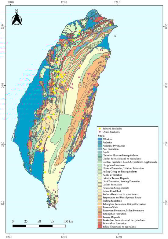
Figure 2. Locations of the 42 sedimentary rock boreholes used in this study, selected from the 88 boreholes drilled during Taiwan’s 2010–2021 mountainous groundwater exploration program.

In addition, the previous groundwater resource exploration project [23] conducted seven in situ investigations at each borehole, including fluid conductivity logging, electrical well logging, groundwater velocity measurement, temperature profiling, borehole imaging, pumping tests, and double-packer hydraulic testing, to collect hydrogeological data. To develop a model for estimating the hydraulic conductivity of mountainous formations along boreholes, this study used data from only four of the seven available tests for analysis: electrical well logging, fluid conductivity logging, double-packer hydraulic testing, and borehole imaging. The electrical well-logging data utilized in this study primarily focuses on four signal types: SP, SNR, LNR, and SPR. Fluid conductivity logging primarily measures pore–water conductivity, which is subsequently converted to fluid resistivity (FR) values. Additionally, the electrical well logging and fluid conductivity logging provided high-resolution data with a one-centimeter sampling interval, aligning with the study’s objective of capturing detailed subsurface variations. For the double-packer hydraulic test in each borehole, data samples were extracted from segments tested with the double packers at 1.5 m intervals, yielding a total of 124 test samples.

Finally, to ensure the quality of the geophysical data (SP, SNR, LNR, SPR, and FR), core logs and borehole imaging were used to verify whether the recorded geophysical responses corresponded with the actual lithological characteristics. The collected data serve as the foundation for correlating electrical geophysical parameters (SP, SNR, LNR, SPR, and FR) with hydraulic conductivity. By applying statistical methods, these correlations can be used to develop robust predictive models for estimating hydraulic properties in sedimentary rock formations.

2.2. Data Processing and Investigation of the Influence of Drilling Mud on Water Resistivity Data

The analyzed data collected in this study were primarily derived from in situ downhole geophysical investigations. Given the inherent variability of field measurement environments and conditions, the recorded data may contain anomalies. Once such anomalies were identified, it was generally not feasible to remeasure or correct the data. Therefore, this study first reviewed the original signal values and cross-referenced them with core imagery to filter out abnormal data. For data exhibiting apparent anomalies, those data were excluded to ensure the reliability of subsequent analyses. Additionally, the study attempted to classify the patterns of these anomalies along the vertical profile and inferred their possible causes. This step improves the accuracy of the subsequent modeling process. Insights from this data-processing approach could also inform the formulation of operational guidelines for downhole geophysical logging, thereby enhancing the quality of acquired data.

In addition, among the five types of borehole logging signals collected, fluid conductivity values were used to derive the resistivity of the pore water (i.e., the reciprocal of fluid conductivity). By integrating this value with formation resistivity, the formation factor (F) can be calculated and further correlated with hydraulic conductivity. However, as noted in the literature review section, the resistivity of pore water can be affected by drilling mud, leading to inaccurate estimates of the formation factor F and, in turn, weakening its relationship with hydraulic conductivity. To address this, the study investigated fluid conductivity in each borehole. Generally, more turbid groundwater corresponds to higher fluid conductivity (and thus lower resistivity). When formation water was contaminated by drilling mud, turbidity increased. The initial investigation evaluated whether the average fluid conductivity values across the borehole exhibited any anomalies. Subsequently, the variation of fluid resistivity with depth in each borehole was examined. Suppose a trend of decreasing resistivity with depth was observed. In that case, it may indicate that formation water has been increasingly influenced by drilling mud, with fine particles settling and degrading water quality at greater depths, thereby increasing fluid conductivity and lowering water resistivity.

Inspection of each borehole allowed identification of resistivity patterns reflecting drilling mud influence, enabling an assessment of the extent of mud contamination in the dataset. Finally, an analysis was conducted to determine whether the inclusion of mud-affected samples impacts the establishment of the relationship between formation factors and hydraulic conductivity.

2.3. Correlation Analysis

Correlation analysis was used to assess the strength and direction of relationships among two or more variables. Variables involved in the analysis include hydraulic conductivity and various geophysical signals (SP, LNR, SNR, SPR, FR, and F). Each geophysical signal data correlated with hydraulic conductivity data to explore various relationships, which can be beneficial for developing a reliable hydraulic conductivity estimation model. Hydraulic conductivity data were primarily derived from double-packer hydraulic tests conducted at 1.5 m intervals, whereas geophysical signals were obtained from borehole logging measurements with a spatial resolution of 1 cm. Given that each double-packer test represents a 1.5 m interval, approximately 150 geophysical data points were available per section. To ensure comparability between the datasets, the 150 geophysical measurements within each interval were averaged to yield a representative signal value, which was then used in further analyses.

To investigate the connections between geophysical signals and hydraulic conductivity, a series of bivariate correlation analyses was conducted. Both Pearson’s correlation (a parametric statistical method) and Spearman’s rank-order correlation (a non-parametric approach) were applied to evaluate the degree of association between each geophysical parameter and the hydraulic conductivity values. Prior to these analyses, the normality of each geophysical dataset was assessed using the Shapiro–Wilk test to determine the appropriate correlation technique. When the dataset met the normality assumption, Pearson’s correlation coefficient was used to quantify the relationship; otherwise, Spearman’s correlation coefficient was adopted. After calculating the correlation values, the results were interpreted based on Cohen’s criteria [24], which categorize the strength of the correlation as follows:

$$\mathrm{S}=\left\{\begin{array}{c}High r\ge 0.5\\ Medium 0.5>r>0.3\\ Low 0.1\le r\le 0.3\end{array}\right.$$

(1)

where S indicates the strength of the association, and r refers to the calculated correlation coefficient from either method. All statistical analyses were conducted using SPSS 24, a commercial statistical software package.

2.4. Data Clustering Using SP Logs

The purpose of data clustering was to ensure that the hydraulic conductivity values of the double-packer test intervals could be effectively correlated with the averaged resistivity values. The simplest way to perform clustering is to classify samples into a single lithology. However, in this study, the lithology of the tested packer intervals was determined by geologists’ interpretations, in which the dominant lithology within each interval was designated as representative, while minor lithological components were neglected. When such unaccounted lithologies do exist within a double-packer test interval, they may significantly affect the relationship between resistivity data and hydraulic conductivity, particularly in complex geological environments (e.g., Taiwan’s mountainous regions). This could prevent the establishment of reliable relationships between resistivity and hydraulic conductivity. To address this issue, this study proposes using SP signals to avoid subjectivity in geological interpretations when defining the dominant lithology of each test interval. As illustrated in the schematic diagram in Figure 3, the SP signal variation with depth is shown for a 1.5 m double-packer test interval. A larger ΔSP within this interval indicates that the geologist’s description of a uniform lithology is inconsistent with the actual subsurface conditions. By utilizing scientific signal data, variations in lithology within each double-packer interval can be more accurately captured, enabling the selection of reliable sample datasets for constructing robust resistivity–hydraulic conductivity correlations. The theoretical basis for adopting SP as a screening tool is described below.

Figure 3. Conceptual diagram illustrating SP variation (ΔSP) within a 1.5 m double-packer interval and its use in identifying lithologic heterogeneity and electrochemical contrast.

The SP signals are measured by the electrical logging tool as the potential difference between a fixed surface electrode and formation electrodes. Since sodium ions in formation water diffuse from zones of high concentration to those of low concentration, when the salinity of the formation water is higher than that of the drilling mud, sodium ions migrate from the high-salinity formation water to the low-salinity drilling fluid, thereby generating spontaneous potential variations. The curve of SP variations with depth is called the SP log and provides insights into lithology and permeability. Because shales generally have low permeability, ion exchange due to mud infiltration (filtration) is limited, leading to minimal potential changes. Thus, SP logs typically display a straight line in shale intervals, known as the shale baseline. In contrast, sandstones are more permeable, and ion exchange induced by mud infiltration is more pronounced, resulting in significant potential differences. Generally, when formation water salinity exceeds mud salinity, sandstone layers exhibit more negative potentials than shale, causing the SP curve to shift to the left (toward more negative potentials). Therefore, based on the characteristic behavior of SP signals, variations in SP values can be used to determine dominant lithology within boreholes or to identify vertical lithological changes within specific intervals. This approach serves as an alternative to lithological classification solely based on core records for data clustering.

Based on the theoretical foundation outlined above, SP has the potential to reflect ion-exchange processes between groundwater and drilling mud, thereby enabling lithological classification. Accordingly, a two-stage data screening method was designed to categorize sample groups for exploring the relationship between rock mass hydraulic conductivity and various resistivity parameters (SNR, LNR, and SPR). The procedure can be implemented using the following steps:

A.

Step 1: Input data preparation

(a)

Extract hydraulic conductivity (K) values from double-packer tests at 1.5 m intervals.

(b)

Average SP, SNR, LNR, and SPR log values over each 1.5 m test interval to obtain representative electrical signals.

(c)

For each interval, record both the average SP value and the SP variation (ΔSP), defined as the difference between the maximum and minimum SP within the interval.

B.

Step 2: Initial SP-based grouping (Stage 1)

(a)

Define candidate SP ranges centered around SP = 0 mV (for example: −100–0 mV, 0–100 mV, 100–200 mV, and combined ranges such as −100–60 mV).

(b)

Assign each double-packer interval to its corresponding SP range based on the average SP value.

(c)

For each SP range that contains at least 10 samples (based on the preliminary testing) to maintain statistical stability, compute the correlation between K and each resistivity signal (SNR, LNR, SPR).

(d)

Identify the optimal SP range that yields the strongest, most stable correlation and the best electrical signal (SNR, LNR, or SPR).

C.

Step 3: ΔSP-based refinement (Stage 2)

(a)

Within the optimal SP range from Stage 1, calculate ΔSP for each interval and classify intervals into candidate ΔSP bands (for example: >5 mV, 5–30 mV, 5–20 mV, 5–15 mV, and 5–10 mV).

(b)

For each ΔSP band, perform regression analysis between the best electrical signal and K and compute the coefficient of determination (R2).

(c)

Select ΔSP bands that produce both high R2 and geologically reasonable behavior.

D.

Step 4: Final dataset definition and model construction

(a)

Define the Stage 1 dataset as all intervals within the optimal SP range. This dataset supports the general predictive model (Model S1).

(b)

Define the Stage 2 dataset as intervals that satisfy both the SP range (Stage 1) and the selected ΔSP band. This dataset supports the high-precision model (Model S2).

In summary, by developing this SP-based data screening methodology, the study provides a scientific approach to overcoming the limitations of subjective lithological classification and improving the robustness of modeling hydraulic conductivity from geophysical resistivity signals.

2.5. Establishing the Relationship Between Resistivity Signals and Hydraulic Conductivity

By integrating the screening results from Section 2.4, the optimal resistivity signal (estimation factor) among the three tested signals, along with the corresponding SP-based sample screening interval, was identified. Regression analysis was then applied to establish a predictive model relating the selected resistivity signal to hydraulic conductivity. The goodness-of-fit of each developed model was evaluated using the coefficient of determination (R²) between hydraulic conductivity and the estimation factor. A higher R² indicates stronger explanatory power of the model for data variability, thus reflecting better model performance. Once the regression model was established, statistical methods were employed to verify its reliability.

To ensure the robustness of the regression models, two statistical evaluations were performed: (1) verification of regression assumptions for residuals—normality (Kolmogorov–Smirnov test), homoscedasticity (Spearman rank correlation), and independence (Durbin-Watson statistic); and (2) examination of model significance using the F-test and corresponding p-values. The optimal regression model for predicting rock mass hydraulic conductivity was then identified from these results. The aforementioned regression and statistical analyses were performed using the commercial software SigmaPlot 14.5.

3. Results

3.1. Data Processing Result

To ensure that the estimation model established in this study was built on a solid data foundation, a quality check was first conducted on 124 sets of double-packer hydraulic test data collected from 42 boreholes, together with five types of downhole geophysical logging data (SP, LNR, SNR, SPR, FR) corresponding to the tested intervals. According to the inspection results, certain boreholes exhibited abnormal signal values in the geophysical logging data within intervals corresponding to the double-packer hydraulic tests. Table 1 summarizes the patterns of abnormal signal values, which include negative values, zeros, −9999, −999, 1200, and values far outside the expected signal range. Ultimately, 10 abnormal samples (approximately 8% of the dataset) were excluded. Notably, most of these abnormal samples corresponded to the shallowest test intervals near the ground surface, suggesting that particular caution is required when using logging data from shallow depths in future studies.

Table 1. Types of abnormal values detected in the borehole logging signals and their corresponding patterns.

Type of Signals	Abnormal Patterns
SP	−99,999, −999, 5062
SNR	Negative value, 12,000, 0
LNR	Negative value, 12,000, 0
SPR	Negative value, 12,000, 0
FR	Negative value, 0, 657

In addition, the fluid resistivity profiles with depth were examined across the boreholes. Two distinct distribution patterns were observed: (1) FR values that decrease markedly with borehole depth (e.g., borehole 104W01, Figure 4a), and (2) FR values that remain essentially constant regardless of depth (e.g., borehole 103W02, Figure 4b). Among the 39 boreholes with usable data, 25 showed a decreasing trend in FR values with depth, accounting for approximately 64% of the dataset. This decreasing trend is interpreted as resulting from particle settling in the drilling mud, which increases water turbidity with depth, thereby elevating fluid conductivity and reducing resistivity. In Figure 4, the red-marked symbols denote the test intervals of the double-packer hydraulic tests. To establish the correlation between formation factor and hydraulic conductivity, three parameters are required: formation resistivity, pore water resistivity, and the hydraulic conductivity of the tested interval. Theoretically, pore water resistivity is not strongly dependent on depth (Figure 4b). However, when borehole water is influenced by mixing between drilling mud and formation pore water, the resulting profile resembles that in Figure 4a. Consequently, the measured fluid resistivity may deviate from the actual formation pore–water resistivity, leading to discrepancies in the calculation of the formation factor and weakening the correlation with hydraulic conductivity. Section 3.2 presents the comparison results of this issue.

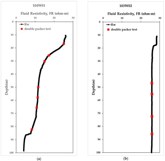
Figure 4. Examples of fluid-resistivity (FR) profiles. (a) Decreasing resistivity with depth due to drilling mud contamination; (b) stable resistivity with depth indicating minimal mud influence.

3.2. Correlation Analysis for Various Well Logging Signals with Hydraulic Conductivity

The correlation analysis revealed relationships between individual borehole logging signals and hydraulic conductivity, highlighting the differing sensitivities of geophysical signals to subsurface hydraulic properties. This correlation outcome can be used to explore potential predictors that reflect rock mass permeability to establish subsequent estimation models. Another correlation study evaluated the influence of mud-affected pore–water resistivity on the relationship between formation factors and hydraulic conductivity (K). All correlation interpretations followed Cohen’s [19] classification of bivariate correlation coefficients. All analyzed results are summarized here.

(a)

Spontaneous Potential (SP):

Correlations between SP and K were consistently very weak across all sedimentary rock samples and lithologic groups (Table 2). In addition, SP is the weakest hydraulic indicator among all evaluated logs. The possible reason is that K reflects how easily water flows through pore spaces or fractures, and is governed by pore-size distribution, connectivity, fracture aperture, tortuosity, and effective stress. In contrast, SP is primarily an electrochemical potential generated by contrasts in lithology, ion mobility, and water salinity formation. These two properties are linked only indirectly and often inconsistently.

Table 2. Correlation coefficients (r) between hydraulic conductivity (K) and individual geophysical logs (SP, SNR, LNR, SPR, FR) for sandstone, shale, and the combined sedimentary dataset.

	Sandstone	Shale	Sedimentary Rocks
Number of samples	87	27	114
SNR	0.450	0.525	0.489
LNR	0.370	0.453	0.427
SPR	0.458	0.482	0.480
SP	−0.119	0.022	−0.077
FR	0.310	0.288	0.331

(b)

Resistivity Logs (SNR, LNR, SPR):

SNR, LNR, and SPR exhibited moderate positive correlations with K (Table 2). Among them, SPR demonstrated the strongest association, followed by SNR, while LNR showed the weakest. The differences are attributed to differences in the sensitivities of the resistivity signals to fracture structures. Despite this variation, all three resistivity logs demonstrated potential as predictive factors. In addition, for correlation analysis across lithologic groups, regardless of resistivity log type, shale consistently shows stronger correlations with hydraulic conductivity than sandstone, whereas the mixed-lithology group falls between the two single-lithology categories. Nevertheless, the differences in correlation strength among the lithologic groups are relatively minor. Shale shows higher resistivity log correlations because its electrical and hydraulic properties change uniformly with compaction, whereas K for sandstone is dominated by fractures and pore-throat variability that resistivity logs cannot sense.

(c)

Fluid Resistivity (FR):

FR maintained a consistent moderate positive correlation with K across lithologies (Table 2). However, the correlation was weaker than that of the original resistivity logs, suggesting limited predictive value.

(d)

Formation Factors (FS, FL, FP):

The correlations of original resistivity logs (SNR, LNR, SPR) were compared with those of derived formation factors (FS, FL, FP) that combine fluid resistivity (FR) with each resistivity log. As shown in Table 3, correlations between K and formation factors were considerably lower than those obtained with the original resistivity logs. This decline is interpreted as a result of FR measurements reflecting mixed drilling fluid and formation water, rather than the true pore–water resistivity assumed in Archie’s law. Consequently, formation factors failed to establish strong relationships with K.

Table 3. Comparison of correlations between hydraulic conductivity (K) and resistivity signals versus formation factors, demonstrating the effect of drilling mud–distorted pore–water resistivity.

Resistivity	r	Formation Factor	r
SNR	0.450	FS (SNR/FR)	0.164
LNR	0.370	FL (LNR/FR)	0.079
SPR	0.458	FP (SPR/FR)	0.130

Overall, original resistivity logs (SNR, LNR, and SPR) show moderate positive correlations with K and can therefore serve as primary predictive variables for estimating rock mass hydraulic conductivity. Conversely, SP and FR are not suitable as primary predictors; however, each parameter remains useful for data screening. SP serves as a lithologic/electrochemical indicator. FR’s principal value is identifying mud-contaminated intervals or anomalies.

3.3. Data Clustering Results

The SP signal was used to overcome geologists’ subjectivity in determining the dominant lithology within double-packer test intervals. By employing objective geophysical data, lithological variations across intervals can be more accurately identified, allowing for the selection of reliable samples to construct robust resistivity–hydraulic conductivity relationships. Examination of sandstone and shale samples (Figure 5) reveals that most SP values fall within 0–300 mV, with sandstones exhibiting a wider range. Notably, only one shale sample recorded a negative SP, consistent with theoretical expectations that sandstones tend to exhibit more negative potential, whereas shales are relatively positive. However, some sandstone SP values exceeded those of shale, indicating the potential of SP signals to distinguish samples more effectively than geologists’ lithologic classifications, thereby allowing for more objective data grouping.

Figure 5. Distribution of spontaneous potential (SP) values for sandstone and shale. Sandstone exhibits a wider SP range, reflecting variable electrochemical and lithologic conditions.

Because SP reflects ion-exchange processes between groundwater and drilling mud, such a signal offers potential for lithologic classification. A two-stage filtering strategy was therefore applied to investigate how resistivity signals respond to hydraulic conductivity under different sample subsets, forming the basis for predictive modeling of rock mass permeability.

• Stage 1: Grouping by SP intervals

For each 1.5 m double-packer interval, the average SP value was adopted as the representative interval signal. Samples were initially grouped into 100 mV intervals centered on SP = 0 mV. Correlations between potential predictive factors (SNR, LNR, and SPR) and K were evaluated across different voltage ranges. As summarized in Table 4, the [−100 mV, 0], [0, 100 mV], and [100 mV, 200 mV] groups revealed that SPR had the strongest correlations with K, reflecting its higher sensitivity to fractures. Among the three ranges, [−100 mV, 0] yielded the strongest correlation (r = 0.879), followed by [0, 100 mV] (r = 0.583), and [100, 200 mV] (r = 0.316). All filtered groups demonstrated stronger correlations than the unfiltered dataset, highlighting the importance of SP-based screening. Additional grouping using SP < 0 and SP > 0 samples did not further improve correlations. Optimization of both sample size and correlation strength identified the range of [−100 mV, 60 mV] as optimal, yielding 25 samples with a correlation of r = 0.858, substantially higher than that of the unfiltered dataset.

Table 4. Correlation coefficients (r) between resistivity signals (SNR, LNR, SPR) and hydraulic conductivity under different SP-based grouping intervals.

Selected Interval of SP Values	Unfiltered	<0	>0	(−100, 0)	(0, 100)	(100, 200)	(0, 60)	(−100, 60)
Number of samples	114	16	98	10	31	44	15	25
r(SNR)	0.489	0.547	0.482	0.503	0.583	0.263	0.75	0.714
r(LNR)	0.427	0.200	0.462	0.115	0.607	0.248	0.639	0.518
r(SPR)	0.480	0.656	0.476	0.879	0.583	0.316	0.804	0.858

Note: SP = spontaneous potential (mV); SNR = short normal resistivity; LNR = long normal resistivity; SPR = single-point resistance.

• Stage 2: Filtering by SP variation (ΔSP)

Regression analysis of SPR–K for the Stage 1 filtered dataset produced a power-law fit with R² = 0.716, considered reliable for engineering applications. To further enhance predictive accuracy, the variation of SP (ΔSP), defined as the difference between maximum and minimum SP values within each test interval, was used as an advanced filtering criterion. Table 5 presents correlations under five ΔSP ranges: [5 mV, maximum], [5 mV, 30 mV], [5 mV, 20 mV], [5 mV, 15 mV], and [5 mV, 10 mV]. Excluding samples with ΔSP < 5 mV increased R² to 0.856. Further restricting the ΔSP upper bound to [5 mV, 30 mV] yielded an R² of 0.866, and progressively narrowing the upper bound further increased R², reaching 0.946 for [5 mV, 10 mV].

Table 5. Coefficients of determination (R²) for SPR–K relationships under different ΔSP filtering thresholds, showing the effect of electrochemical contrast on model performance.

ΔSP (mv)	R2	Sample Quantity
N.A.	0.7156	25
>5	0.8559	15
(5, 30)	0.8664	13
(5, 20)	0.8600	12
(5, 15)	0.8908	9
(5, 10)	0.9456	6

Note: ΔSP = SP variation within the 1.5 m packer interval (mV).

Two conclusions arise from these results. First, larger ΔSP values indicate greater lithologic heterogeneity within test intervals, which negatively affects the establishment of reliable relationships between resistivity and hydraulic conductivity. Accordingly, smaller ΔSP ranges produced better correlations. Second, contrary to theoretical expectations, excluding samples with ΔSP < 5 mV improved model performance. The influence of drilling additives explains this outcome: when drilling mud properties reduce ion-exchange contrasts with formation water, SP variations diminish, leading to ΔSP values < 5 mV that poorly represent lithologic differences. These samples, therefore, introduce noise and degrade model accuracy. Importantly, this ΔSP < 5 mV cutoff is not proposed as a universal or theoretical threshold, but rather as a data-driven criterion specific to the hydrogeological and drilling conditions of this study area. Thus, this particular threshold should be tested before application in other regions.

The analysis demonstrates that SP-based filtering is essential for improving the correlation between resistivity logs and hydraulic conductivity. Stage 1 filtering by SP interval reduces lithologic subjectivity, while Stage 2 filtering by ΔSP effectively eliminates noisy samples influenced by drilling mud or heterogeneous lithology. Although sample size decreases, the resulting dataset exhibits clearer signal–property relationships, thereby enhancing the reliability of permeability prediction models.

3.4. Establishment of Hydraulic Conductivity Estimation Models

Based on the two-stage filtering of SP signal data described in Section 3.3, two predictive models (S1 and S2) for estimating hydraulic conductivity (K) using single-point resistance (SPR) signals were constructed. The first model (S1) was established by filtering data according to the SP intervals, with the optimal range identified as [−100 mV, 60 mV], yielding 25 samples. Regression analysis between SPR and K (Figure 6) indicated that the best-fit equation is a power law (Equation (2)), with a coefficient of determination (R²) of 0.7156. Model S1 thus represents an approach that maximizes sample size.

$$\mathrm{K}=7\times {10}^{-13}{\mathrm{SPR}}^{3.430}$$

(2)

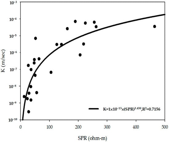
Figure 6. SPR–K regression for Model S1 (25 samples), showing the general predictive relationship after SP-based screening.

The second model (S2) was developed using the same Stage 1 dataset and refined with an additional filtering criterion based on SP variation (ΔSP). Samples with ΔSP within [5 mV, 10 mV] were retained, resulting in six samples. Regression analysis between SPR and K (Figure 7) also yielded a power-law relationship (Equation (2)), with a markedly higher coefficient of determination (R² = 0.9456). The Model S2, therefore, reflects an approach that emphasizes optimal predictive performance.

$$\mathrm{K}=2\times {10}^{-14}{\mathrm{SPR}}^{3.505}$$

(3)

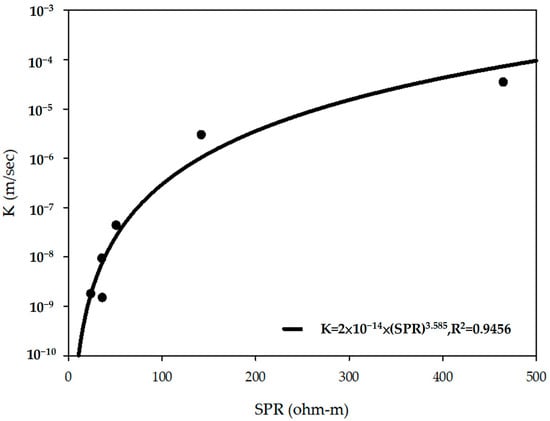
Figure 7. SPR–K regression for Model S2 (6 high-quality samples), illustrating the stronger correlation obtained after additional ΔSP filtering.

A comparison between the two models reveals distinct trade-offs. Model S1 relies on average SP values from double-packer intervals, eliminating reliance on geologists’ lithologic interpretations and enabling rapid sample screening. However, the influence of groundwater chemistry and lithologic heterogeneity within test intervals reduces predictive accuracy. In contrast, Model S2 isolates samples minimally affected by drilling mud or lithologic heterogeneity, thereby achieving substantially higher precision.

Although the coefficient of determination (R²) provides a preliminary measure of model performance, additional statistical tests were applied to ensure the reliability of the results. Model validity was further assessed using the F-test for overall regression significance, along with residual diagnostics for independence (Durbin–Watson test), normality (Kolmogorov–Smirnov test), and homoscedasticity (Spearman’s rank correlation).

For Model S1 (Table 6), the F-test confirmed statistical significance of the predictor variable, indicating predictive capability. Residual independence was verified as the Durbin–Watson statistic (D = 2.010) exceeded the upper critical value (D_u = 1.210, at the 1% level of significance) for n (sample size) = 25 and k (regressor) = 1 [25]. Normality was confirmed with a K–S test (p = 0.8938, p > 0.005), and homoscedasticity was supported by a Spearman correlation (p = 0.942, p > 0.005). These results indicate that Model S1 meets all statistical assumptions, confirming its predictive validity.

Table 6. Statistical validation results (independence, normality, homoscedasticity, and F-test) for the two hydraulic conductivity prediction models (S1 and S2).

Models	Independence (D–W Statistic)	Normality (K-S Statistic/ p–Values)	Constant of Variance (Spearman/ p–Values)	F Test Statistic
				F Ratio	p–Values
S1	2.010	0.894	0.942	58.098	<0.0001
S2	1.210	0.852	0.787	65.094	0.001

For Model S2 (Table 6), the F-test again confirmed statistical significance. The Durbin–Watson statistic (D = 1.210) exceeded the upper critical value (D_u = 1.142, at the 1% level of significance) under n (sample size) = 6 and k (regressor) = 1 [25], indicating residual independence. Normality was confirmed with a K–S test (p = 0.852, p > 0.005), while homoscedasticity was supported by a Spearman correlation (p = 0.787, p > 0.005). Thus, Model S2 also satisfies all statistical assumptions, supporting its reliability in predicting hydraulic conductivity. Despite the small sample size (n = 6), the ΔSP = 5–10 mV subset corresponds to intervals with the most uniform lithology and least mud-induced disturbance. The reduction in sample size, therefore, reflects geological filtering rather than a statistical perspective. In such homogeneous intervals, the SPR–K mechanism is theoretically expected to be stronger due to reduced variability in pore structure and reduced clay effects. Future work will incorporate additional boreholes to enlarge the ΔSP-restricted dataset, allowing validation and potential refinement of Model S2 while maintaining its physically grounded filtering criteria. This effort facilitates progress toward developing a more broadly generalizable prediction model.

Finally, representative diagnostic figures using SPSS 24 were generated to visually assess the adequacy of the first regression model (S1) and to complement the numerical statistical tests performed by SigmaPlot. The residual vs. fitted plot (Figure 8a) shows a random and pattern-less distribution of standardized residuals, indicating that no systematic structure, heteroscedasticity, or dependence is present. The probability–probability (P–P) plot (Figure 9a) demonstrates that the empirical cumulative distribution of the residuals aligns closely with the expected theoretical normal distribution, confirming that the normality assumption is reasonably satisfied. Together, these diagnostic figures provide intuitive support for the validity of the regression models and substantiate the statistical diagnostics reported in this study. For the second regression model (S2), the diagnostic residual vs. fitted (Figure 8b) and P–P plots (Figure 9b) also indicate no observable patterns, heteroscedasticity, or deviations from normality, confirming that this model similarly satisfies the assumptions required for the regression.

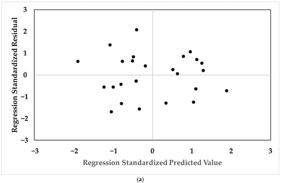
Figure 8. The residual vs. fitted plots: (a) Model S1; (b) Model S2.

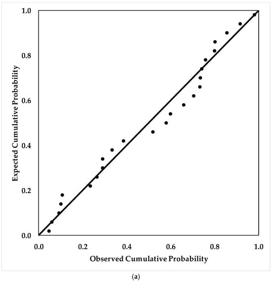
Figure 9. The probability–probability (P–P) plots: (a) Model S1; (b) Model S2.

3.5. Engineering Workflow and Practical Implementation

To support engineering use, the proposed SP-assisted screening and SPR–K modeling approach was formulated into a practical workflow comprising five steps: (1) acquisition of borehole electrical logs and packer-test K values, (2) SP-based interval grouping and ΔSP filtering to isolate electrochemically stable intervals, (3) selection of the appropriate predictive model (general or high-precision), (4) generation of a continuous K profile along the borehole, and (5) interpretation of the estimated K distribution to identify permeable fracture zones, groundwater-yielding intervals, and hydraulic heterogeneity relevant to project design.

The workflow’s reliability was examined using internal statistical diagnostics, including tests of independence, normality, and homoscedasticity, and significance testing of model parameters. Geological consistency checks—such as alignment with lithologic logs, observed fracture density, and mud-invasion patterns—provided additional validation. These steps demonstrate that the workflow can be readily implemented in engineering settings and can reduce dependence on extensive hydraulic testing.

4. Discussion

4.1. Accuracy and Reliability of Electrical–Hydraulic Relationships

The results of this study demonstrate that direct resistivity logs (particularly SPR) provide the strongest and most stable correlations with hydraulic conductivity in fractured and clay-rich sedimentary formations. This finding aligns with previous hydrogeophysical research showing that resistivity measurements are susceptible to pore-fluid conductivity, fracture connectivity, and lithologic contrasts under electrochemically stable conditions [10,11,12]. Earlier studies likewise reported that SPR is particularly effective in identifying permeable structures in consolidated rock because it reflects conductive pathways controlling groundwater flow [13,14]. The enhanced SPR performance after SP-assisted screening in this study is consistent with these findings and underscores the importance of minimizing electrochemical disturbance during interpretation.

Formation factor approaches showed weak predictive capability, as expected in clay-rich or drilling mud-affected formations where the assumptions underlying Archie’s law do not hold. Clay mineral surfaces generate membrane potential and ion-exchange behavior that distort the relationship between bulk resistivity and pore–water resistivity [21,22]. Additionally, drilling mud invasion can significantly alter pore–water chemistry, rendering formation factor estimates unreliable. Similar limitations have been reported in sedimentary rock investigations in Taiwan, supporting the poor performance observed here [1].

4.2. Consistency with Previous Literature

The two-stage SP-assisted screening framework introduced in this study improves the physical consistency between resistivity signals and hydraulic behavior. Grouping intervals by average SP reduces lithologic mixing and highlights electrochemical contrasts meaningful for hydraulic interpretation. This concept is consistent with early SP studies that showed SP sensitivity to salinity gradients, clay content, and ion-exchange processes that vary systematically with lithology [8,9]. The clustering behavior observed here, where specific SP ranges correspond to stronger electrical–hydraulic coherence, is therefore supported by long-established electrochemical principles.

Filtering intervals using SP variation (ΔSP) further improves model performance by removing intervals affected by drilling mud disturbances or internal lithologic heterogeneity. Previous work has shown that resistivity–hydraulic relationships strengthen when pore-fluid chemistry remains stable [11,12]. The high-precision model developed under optimized ΔSP conditions (R² = 0.946) is consistent with these findings and demonstrates the effectiveness of ΔSP as a diagnostic indicator of electrochemical reliability.

Overall, the correlations and model improvements presented in this study are strongly supported by established hydrogeophysical theory and prior empirical results. The consistency across independent studies enhances confidence in the robustness and applicability of the proposed workflow.

4.3. Study Limitations and Considerations

Despite the promising results, several limitations warrant consideration. The dataset exhibits lithologic imbalance, with fewer shale intervals than sandstone intervals. Although shale intervals produced stronger correlations, the smaller sample size may limit generalization in shale-dominated formations. Drilling mud invasion also remains a significant challenge; even after SP-based screening, some intervals may retain contamination effects influencing resistivity signals. Similar concerns regarding mud perturbation and its impact on resistivity-based hydraulic models have been noted in previous studies [15,17].

Lastly, although supported by electrochemical principles, the SP grouping thresholds and ΔSP criteria derived here are based on site-specific behavior. Additional testing in broader geological settings is necessary to confirm the transferability of these thresholds.

4.4. Contribution to Sustainable Development Goals (SDGs)

This study directly contributes to SDG 6 (Clean Water and Sanitation) by improving the ability to rapidly characterize groundwater-bearing formations in mountainous regions, where water supply security is a concern during drought. The proposed method provides a cost-effective means to generate hydraulic conductivity profiles without relying on extensive pumping tests. The work also supports SDG 9 (Industry, Innovation and Infrastructure) by offering a practical engineering workflow that enhances subsurface investigation efficiency, aiding in tunnel design, slope stabilization, and rural water-supply planning.

5. Conclusions

The present investigation highlights the feasibility of utilizing borehole geophysical logging, with particular emphasis on spontaneous potential (SP) and single-point resistance (SPR) measurements, for estimating hydraulic conductivity in geologically complex sedimentary rock environments of Taiwan’s mountainous regions. By addressing the limitations of Archie’s law in clay-rich formations and mitigating the influence of drilling mud on pore–water resistivity, this study establishes a more reliable framework for electrical–hydraulic conductivity relationships. The significant findings can be summarized as follows:

• This study demonstrates that borehole electrical logging, when combined with a targeted SP-based screening strategy, can substantially improve the estimation of hydraulic conductivity in Taiwan’s complex sedimentary rock formations.
• Quantitative analysis of 124 double-packer intervals shows that formation factor–based predictions yield weak relationships with hydraulic conductivity due to drilling mud alteration of pore–water resistivity and the presence of clay, both of which disrupt the assumptions of Archie’s law. These findings align with earlier work in fractured and heterogeneous rocks, where formation factors also showed limited predictive capability.
• In contrast, direct resistivity signals—particularly single-point resistance (SPR)—provide markedly stronger associations with hydraulic conductivity. After applying the two-stage SP screening procedure, the SPR–K relationship becomes substantially more transparent, yielding regression models with R² = 0.716 for the general model and R² = 0.946 for the high-precision model. These results underscore that reducing lithologic heterogeneity and electrochemical instability enhances the physical consistency between resistivity behavior and hydraulic properties. Such improvements are consistent with previous hydrogeophysical studies reporting that direct resistivity measurements outperform derived parameters in consolidated or clay-affected formations.
• Overall, the data confirm that the proposed SP-assisted screening framework provides a reliable, physically grounded approach for identifying intervals in which resistivity signals meaningfully reflect hydraulic behavior. The resulting models offer a practical tool for generating continuous hydraulic conductivity profiles in sedimentary bedrock aquifers—an outcome valuable for subsurface characterization in mountainous regions where conventional testing is operationally challenging.

6. Recommendations

Future research and engineering applications can extend the findings of this work through the following directions:

• Expanding data coverage by incorporating additional boreholes from different sedimentary settings to evaluate the generalizability of the SP-based screening thresholds.
• Integrating complementary geophysical logs, such as acoustic televiewer and full-waveform resistivity tools, to further characterize fracture geometry and improve prediction accuracy.
• Refining ΔSP criteria through controlled drilling mud experiments to quantify the influence of mud properties on SP behavior and enhance transferability to other regions.
• Conducting cross-hole or multi-borehole validation, enabling assessment of model performance at larger spatial scales relevant to groundwater extraction or engineering design.
• Applying the workflow to hydrogeologic or engineering projects, including screen placement, leakage detection, tunnel inflow assessment, and groundwater resource evaluations, to establish standardized operational guidelines.

These recommendations provide a forward-looking pathway to improve both the scientific understanding and the practical deployment of resistivity-based hydraulic conductivity estimation methods in complex geologic environments.

References

- Hsu, S.M.; Liu, G.Y.; Dong, M.C.; Liao, Y.F.; Li, J.S. Investigating formation factor–hydraulic conductivity relations in complex geologic environments: A case study in Taiwan. Water 2023, 15, 3621. [Google Scholar] [CrossRef]
- Gao, Q.; Hasan, M.; Shang, Y.J.; Qi, S.W. Geophysical estimation of 2D hydraulic conductivity for groundwater assessment in hard rock. Acta Geophys. 2024, 72, 4343–4354. [Google Scholar] [CrossRef]
- Lärm, L.; Weihermüller, L.; Rödder, J.; Kruk, J.; Vereecken, H.; Klotzsche, A. Spatial variability of hydraulic parameters of a cropped soil using horizontal crosshole ground penetrating radar. Vadose Zone J. 2025, 24, e20389. [Google Scholar] [CrossRef]
- Dahunsi, J.; Pathirana, S.; Cheema, M.; Krishnapillai, M.; Galagedara, L. Estimating soil hydraulic conductivity from time-lapse ground-penetrating radar data in podzolic soils using the Green-Ampt model. J. Hydrol. 2025, 657, 133059. [Google Scholar] [CrossRef]
- Hsu, S.M. Quantifying hydraulic properties of fractured rock masses along a borehole using composite geological indices: A case study in the mid- and upper-Choshuei river basin in central Taiwan. Eng. Geol. 2021, 284, 105924. [Google Scholar] [CrossRef]
- Shahbazi, A.; Saeidi, A.; Chesnaux, R. A review of existing methods used to evaluate the hydraulic conductivity of a fractured rock mass. Eng. Geol. 2020, 265, 105438. [Google Scholar] [CrossRef]
- Jones, P.H.; Buford, T.B. Electric logging applied to ground-water exploration. Geophysics 1951, 16, 115–139. [Google Scholar] [CrossRef]
- Meidav, T. An electrical resistivity survey for ground water. Geophysics 1960, 25, 1077–1093. [Google Scholar] [CrossRef]
- Page, L.M. The use of the geoelectric method for investigating geologic and hydrologic conditions in Santa Clara County, California. J. Hydrol. 1969, 7, 167–177. [Google Scholar] [CrossRef]
- Urish, D.W. Electrical resistivity-hydraulic conductivity relationships in glacial outwash aquifers. Water Resour. Res. 1981, 17, 1401–1408. [Google Scholar] [CrossRef]
- Huntley, D. Relations between permeability and electrical resistivity in granular aquifers. Groundwater 1986, 24, 466–474. [Google Scholar] [CrossRef]
- Slater, L.; Lesmes, D.P. Electrical-hydraulic relationships observed for unconsolidated sediments. Water Resour. Res. 2002, 38, 31-1–31-13. [Google Scholar] [CrossRef]
- Khalil, M.A.; Ramalho, E.C.; Monteiro Santos, F.A. Using resistivity logs to estimate hydraulic conductivity of a Nubian sandstone aquifer in southern Egypt. Near Surf. Geophys. 2011, 9, 349–356. [Google Scholar] [CrossRef]
- Khalil, M.A.; Santos, F.A.M. Hydraulic conductivity estimation from resistivity logs: A case study in Nubian sandstone aquifer. Arab. J. Geosci. 2013, 6, 205–212. [Google Scholar] [CrossRef]
- Kaleris, V.K.; Ziogas, A.I. Estimating hydraulic conductivity profiles using borehole resistivity logs. Procedia Environ. Sci. 2015, 25, 135–141. [Google Scholar] [CrossRef]
- Asfahani, J. Porosity and hydraulic conductivity estimation of the basaltic aquifer in Southern Syria by using nuclear and electrical well logging techniques. Acta Geophys. 2017, 65, 765–775. [Google Scholar] [CrossRef]
- Kaleris, V.K.; Ziogas, A.I. Using electrical resistivity logs and short duration pumping tests to estimate hydraulic conductivity profiles. J. Hydrol. 2020, 590, 125277. [Google Scholar] [CrossRef]
- Muauz, A.; Berehanu, B.; Bedru, H. An alternative approach using electrical well logging for estimating porosity and hydraulic conductivity in volcanic aquifers of the upper Awash River sub-basin, Ethiopia. J. Hydrol. Reg. Stud. 2025, 60, 102547. [Google Scholar] [CrossRef]
- Lora-Ariza, B.; Silva Vargas, L.; Donado, L.D. Estimation of hydraulic conductivity from well logs for the parameterization of heterogeneous multilayer aquifer systems. Water 2025, 17, 2439. [Google Scholar] [CrossRef]
- Archie, G.E. The electrical resistivity log as an aid in determining some reservoir characteristics. Trans. AIME 1942, 146, 54–62. [Google Scholar] [CrossRef]
- Shen, B.; Wu, D.; Wang, Z. A new method for permeability estimation from conventional well logs in glutenite reservoirs. J. Geophys. Eng. 2017, 14, 1268–1274. [Google Scholar] [CrossRef]
- Waxman, M.H.; Smits, L.J.M. Electrical conductivities in oil-bearing shaly sands. Soc. Pet. Eng. J. 1968, 8, 107–122. [Google Scholar] [CrossRef]
- Geological Survey and Mining Management Agency of Taiwan. Ground-Water Resources Investigation Program for Mountainous Region of Central Taiwan (1/4); Ministry of Economic Affairs: Taipei, Taiwan, 2010.
- Cohen, J.; Cohen, P.; West, S.G.; Aiken, L.S. Applied Multiple Regression/Correlation Analysis for the Behavioral Sciences; Routledge: Abingdon, UK, 2013. [Google Scholar]
- Savin, N.E.; White, K.J. The Durbin-Watson test for serial correlation with extreme sample sizes or many regressors. Econometric 1977, 45, 1989–1996. [Google Scholar] [CrossRef]
Disclaimer/Publisher’s Note: The statements, opinions and data contained in all publications are solely those of the individual author(s) and contributor(s) and not of MDPI and/or the editor(s). MDPI and/or the editor(s) disclaim responsibility for any injury to people or property resulting from any ideas, methods, instructions or products referred to in the content. |
© 2025 by the authors. Licensee MDPI, Basel, Switzerland. This article is an open access article distributed under the terms and conditions of the Creative Commons Attribution (CC BY) license (https://creativecommons.org/licenses/by/4.0/).