


Abstract
Point-wise intensification of daily rainfall extremes over India is well established, yet whether their joint spatial behavior is also changing has not been tested. We address this with 75 years (1951–2025) of 0.25° gridded India Meteorological Department daily rainfall, quantifying June–September (JJAS) extremal dependence through the extremal-coefficient function θ(h) and the dependence range ρ of a Brown–Resnick curve fitted to F-madogram estimates on rank-transformed fields; the rank transform strips out marginal trends, so any surviving signal belongs to the joint structure. The all-India range over the full record is 65.6 km (95% CI 62.0–69.5 km). Across 21 sliding 15-year windows, θ at 50 and 100 km fell significantly (p = 0.033 and 0.010 after serial-correlation correction): extremes co-occur more strongly at the storm scale. The signal is regional: Peninsular India’s dependence range grew from 56 km to 76 km between the 1951–1975 and 2001–2025 blocks, a 36% expansion (p = 0.002), and Central India’s window trend is +1.7 km decade−1 (p = 0.017). Independently, the largest connected daily exceedance cluster expanded in area by roughly 40% (p ≤ 0.0006). A Pettitt test dates the step in the footprint series to 1986 (p ≤ 0.0001), whereas the dependence series show progressive trends without a detectable break. Spatial reorganization is compounding marginal intensification: across Peninsular India, joint flood risk is growing faster than cell-wise return levels indicate.
1. Introduction
Few weather hazards match the destructive reach of daily rainfall extremes in the Indian summer monsoon (June–September, JJAS): a single day of intense, spatially organized rain can flood a densely populated river basin, and such floods recur across the subcontinent. That these extremes are changing is by now well established [1]. Goswami et al. [2] reported that heavy events over Central India grew in both frequency and magnitude during 1951–2000, and later analyses of longer records confirmed significant upward trends in the count of extreme events, superimposed on strong inter-decadal variability [3,4]. Vinnarasi and Dhanya [5] traced shifts in the character of wet and dry spells, while attribution studies indicate that anthropogenic warming has already made extreme daily precipitation over India more probable [6]. Recent syntheses reinforce this picture. A meta-analysis of regional extreme rainfall events across the subcontinent finds their frequency and intensity rising together with their spatial variability, with the increase over Central India tied to synoptic systems and circulation changes [7]; downscaled and bias-corrected CMIP6 projections indicate that the spatial variability of extreme rainfall will grow roughly twice as fast as that of seasonal totals [8], and that the area covered by long-duration extreme events will expand further under continued warming [9]; the north-west of the country, historically the driest part of the monsoon domain, has become markedly wetter since the 1980s in association with Arabian Sea warming and Hadley-cell expansion [10]; and even the timing of peak monsoon rainfall has shifted regionally over the last two decades [11].
Nearly all of this work concerns the marginal rainfall distribution at each location—trends in threshold counts, in annual maxima, or in return levels fitted cell by cell. Yet the damage a monsoon extreme inflicts depends at least as much on how the rain is arranged in space. Confine a 150 mm day to one 25 km grid box, and the problem is local drainage; spread the same intensity coherently across a 50,000 km2 river basin, and the outcome is a regional flood disaster. Roxy et al. [12] pressed this point by demonstrating a threefold increase in ‘widespread’ extreme rain events across Central India—a category defined by its simultaneous extent. Complex-network studies of event synchronization arrive at a similar place from another direction: extreme monsoonal rainfall organizes into coherent spatial patterns that track monsoon depressions and orography [13], and the synchronization reaches global teleconnection scales [14]. None of these studies, though, pins down the dependence between extremes in the formal sense of extreme-value theory, and none asks whether that dependence is itself drifting as the planet warms.
Extreme-value theory supplies the missing framework. For spatial maxima, max-stable processes carry the generalized extreme-value (GEV) distribution over to random fields [15,16,17,18]. Pairwise extremal dependence is then captured by the extremal coefficient θ(h), which rises from 1 under complete dependence towards 2 under asymptotic independence as the separation h grows [19]. There is no need to fit a full max-stable model to estimate it: the F-madogram, a first-order variogram computed on the marginal-transformed field, yields θ(h) directly [20,21]. Accessible software and tutorial treatments of multivariate and spatial extremal dependence have recently made these tools routine [22], and clustering approaches have been proposed to regionalize the extremal dependence structure of rainfall fields into homogeneous sub-domains [23]. The estimator is robust and cheap to compute, and because it acts on rank-transformed data, it is blind to marginal trends—it strips the dependence signal clean of exactly the non-stationarity already documented in the marginal record.
Applications of the spatial-extremes toolkit to India have so far kept the dependence stationary. Athira et al. [24] provide the most recent example: max-stable models fitted to India’s monsoon extremes, with geographic and temporal covariates carried in the margins, documenting return levels that rise and become more localized—but with the dependence structure held constant over time. Outside India, the assumption of a temporally stationary dependence structure has only very recently been relaxed: Maume-Deschamps et al. [25] formulated a space–time max-stable model in which the spatial extremal dependence evolves with time and, applying it to rainfall in southern France, found that dependence to be significantly non-stationary. That work establishes the question as tractable, but it has not been asked of the Indian monsoon. Whether the monsoon’s daily extremes are growing more spatially coherent—dependence range lengthening, joint-event footprints expanding—or whether instead they are fragmenting has, as far as we know, never been tested. The distinction carries real weight. With margins held fixed, growth in the dependence range is by itself enough to raise basin-scale flood risk; when dependence and margins intensify together, the compounding accelerates.
Here we address that gap with an analysis that is deliberately empirical and estimator-driven, based on 75 monsoon seasons of 0.25° gridded daily rainfall covering 1951–2025 [26]. Our objectives are to: (i) establish the marginal extreme-value backdrop—GEV and generalized Pareto distribution (GPD) parameters, return levels, seasonal-maximum trends—against which any change in dependence must be read; (ii) estimate the extremal-coefficient function θ(h) and the associated dependence range ρ over the full period, both for all-India and for five climatic zones; (iii) test whether ρ, the variogram smoothness ν and θ at fixed separations change across 21 sliding 15-year windows, applying Mann–Kendall tests corrected for serial correlation [27,28,29,30] and complementing them with a non-parametric change-point analysis [31]; (iv) pin down where the change occurs by mapping a neighborhood-based dependence range within an early (1951–1975) block and a late (2001–2025) block; (v) check the dependence story against a physically transparent diagnostic—the area covered by the largest connected cluster of local-99th-percentile exceedances; and (vi) translate the detected changes into joint-exceedance probabilities and practical consequences for basin-scale flood risk.
2. Data and Study Region
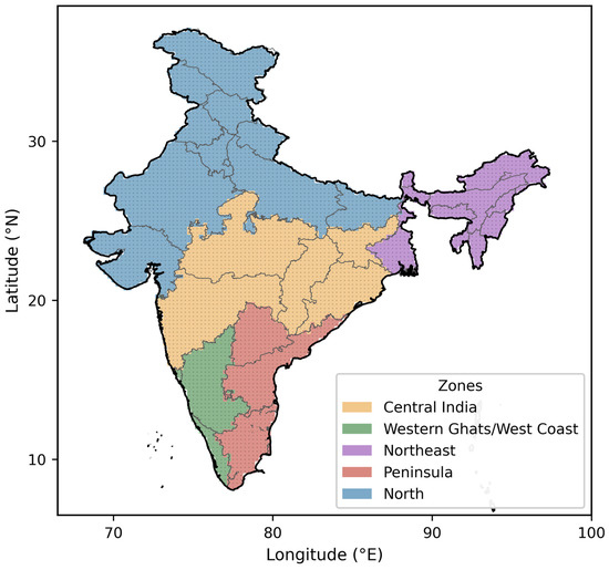
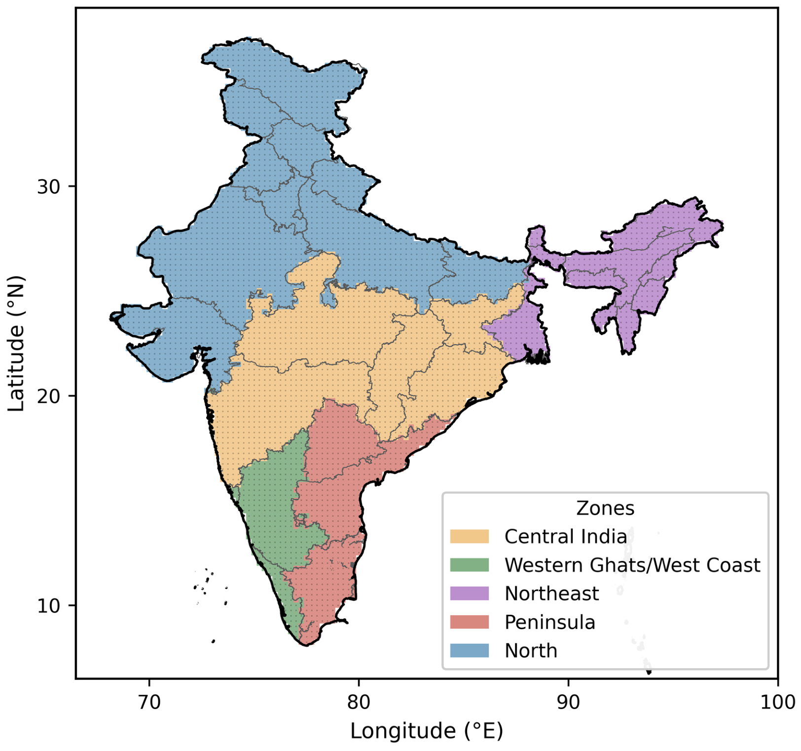
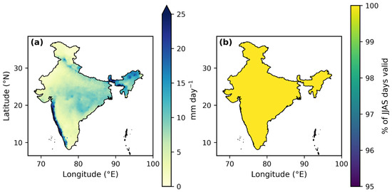
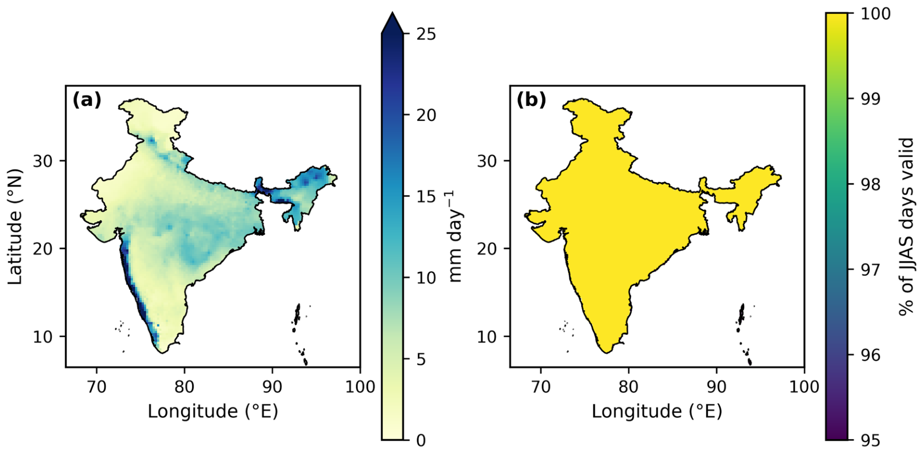
Rainfall data are sourced from the India Meteorological Department (IMD) high-resolution gridded daily product at 0.25° × 0.25° [26], covering the 27,394 days from 1 January 1951 to 31 December 2025. The grid spans 6.5–38.5° N and 66.5–100.0° E (129 × 135 cells). Every statistic in this paper is computed on the JJAS season alone, which contributes 122 days in each of the 75 years (9150 season-days), and on grid cells whose centers lie within the India outer boundary. That boundary contains 4633 cells; 4615 of them report data on every JJAS day, and the other 18 are flagged missing throughout the record—a constant 0.389% of the domain (Table 1). Figure 1 maps the domain and the five zones used in the regional analysis: Central India, Western Ghats/West Coast, Northeast, Peninsula and North. Built by merging state polygons, these zones jointly cover all 4615 usable cells. The JJAS climatology and data availability appear in Figure 2; the west-coast and northeastern rainfall maxima stand out, as does the arid north-west.
Table 1.
Yearly data-quality summary (first and last five years listed; the complete 75-year table is provided with the analysis archive): JJAS day count, missing fraction within the India boundary, and the domain maximum and mean daily rainfall.
Figure 1.
The study domain: IMD 0.25° grid cells (dots), the India outer boundary (black), the state polygons (gray), and the five zones used to compute regional statistics.
Figure 2.
(a) Mean daily JJAS rainfall over 1951–2025. (b) Percentage of JJAS days carrying valid data.
The product is constructed by Shepard’s distance-weighted interpolation of quality-controlled daily gauge reports—a national archive of up to 6955 stations, with between one and four stations drawn from within a 1.5° search radius of each grid point [26,32]. Three properties of this construction matter for what follows. First, interpolation is a smoothing operator: it attenuates point maxima and inflates apparent spatial coherence, so the marginal return levels of Section 4.1 are grid-box rather than point quantities, and the dependence range ρ carries a positive bias relative to the dependence of the underlying point process. Independent evaluations report a substantial underestimation of precipitation over the wettest parts of the country [33] and a reduced ability to capture individual extreme events where the network is sparse, notably in the north-west Himalaya [34]. Second, the bias is spatially structured—largest where gauges are sparse (the trans-Himalayan north-west and parts of the Northeast) and smallest over the Peninsular and Central India, where the network is densest; the recently released station-based ensemble product for India, which quantifies interpolation uncertainty explicitly, shows the same pattern [32]. Third, the gauge network has not been constant through time, so a time-varying interpolation bias is in principle a competing explanation for any trend in ρ. Section 3.3 describes the sensitivity test used to guard against this possibility, and Section 7 sets out why the design of the study makes it unlikely.
3. Methods
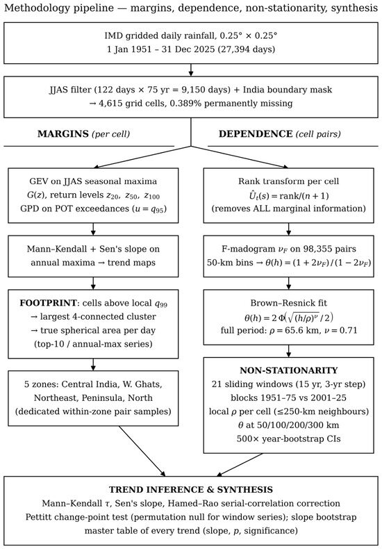
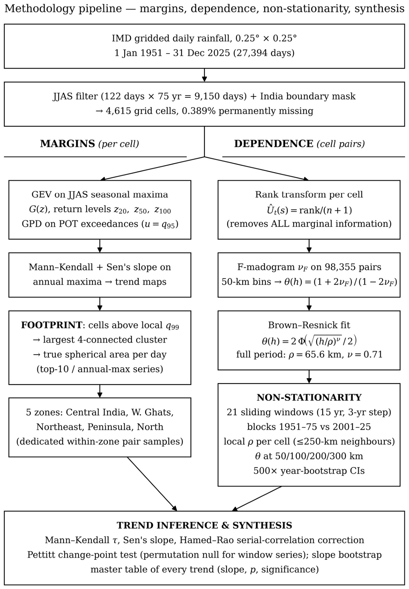
Figure 3 lays out the workflow. Marginal fits come first, for context; each cell’s series is rank-transformed to uniform margins; θ(h) is then estimated via the F-madogram with distance binning and summarized by a parametric dependence fit; finally, the dependence estimation is repeated across sliding windows, blocks and zones. Each stage is set out below.
Figure 3.
Methodology overview. The marginal branch (left) fits the GEV and GPD at every cell, tests the annual maxima for trend, and derives the footprint diagnostic and the zonal pair samples; the dependence branch (right) rank-transforms each cell, computes the pairwise F-madogram in 50 km bins, fits the Brown–Resnick extremal-coefficient curve, and repeats the estimation across 21 sliding 15-year windows, two 25-year blocks and each cell’s ≤250 km neighborhood. Both branches converge on a common inference stage of trend, change-point and bootstrap tests.
3.1. Marginal Extremes
At every cell, we fit the generalized extreme-value distribution to the 75 seasonal (JJAS) maxima [35]:
Here, location μ, scale σ, and shape ξ are obtained by maximum likelihood; at the few cells where the optimizer converged to an unphysical shape (210 of 4615), L-moment estimates were used instead. The T-year return level then follows as
To cross-check the tail in a way less tied to the block-maximum choice, exceedances of the cell-specific 95th percentile u—the peaks-over-threshold (POT) approach—were also fitted with the generalized Pareto distribution:
Per-cell temporal trends in the annual JJAS maxima were evaluated using the Mann–Kendall test together with Sen’s slope (Section 3.4).
3.2. Extremal Dependence: The F-Madogram and θ(h)
The JJAS daily series at each cell is first mapped to uniform margins through its empirical cumulative distribution function (CDF) (ties receive average ranks):
which strips out all marginal information, marginal trends included, so that any temporal signal surviving the transform belongs to the joint structure. For a pair of locations, the F-madogram [20] is defined as half of the mean absolute difference between the transformed values:
and it translates one-to-one into the pairwise extremal coefficient [19]:
θ = 1 corresponds to complete dependence, and θ = 2 to independence. As a parametric summary, we use the extremal-coefficient function of the Brown–Resnick class [17], which is generated by the power-law variogram:
where Φ denotes the standard normal CDF; ρ (km), the dependence range, marks the separation at which γ = 1 and sets a characteristic scale for the decay of extremal dependence; and ν governs the smoothness of that decay. Separations between cell centers are computed as great-circle (haversine) distances:
Estimation rests on a random sample of 98,355 cell pairs, stratified by distance (≤2500 per 50 km bin, separations 22–2000 km). Madogram values for individual pairs are then averaged in 50 km bins, keeping bins with ≥30 pairs:
and the pair (ρ, ν) is obtained through pair-count-weighted least squares:
Uncertainty arises from resampling seasons: entire years are sampled with replacement (500 replicates, fixed seed), the binned θ values are recalculated, and the curve is refitted, yielding percentile confidence intervals for ρ, ν, and θ in each bin. Because a replicate always contains complete monsoon seasons, the strong serial dependence between successive days of a season never straddles replicate boundaries. The resulting intervals are marginal intervals for each individual estimate. When the same bootstrap is applied window by window (Section 3.3), the intervals of neighboring windows are far from independent—successive windows share most of their seasons, so their sampling errors are strongly and positively correlated—and the width of a per-window band must not be read as the uncertainty of a trend across windows; that quantity is estimated separately (Section 3.4).
3.3. Non-Stationarity Design
The entire estimation is rerun across 21 sliding windows of 15 years, each shifted forward by 3 years (1951–1965, 1954–1968, …, 2011–2025), recomputing the ranks within each window. For each window, we keep ρ, ν, and the empirical θ, interpolated to the fixed separations of 50, 100, 200, and 300 km. An independent, window-free contrast is based on two 25-year blocks, 1951–1975 and 2001–2025, compared using paired-bootstrap confidence intervals for the change in ρ. Change is localized by estimating, for each cell, a local dependence range: the F-madogram is evaluated between that cell and every valid neighbor within 250 km (243 neighbors at the median), and a one-parameter Brown–Resnick curve—ν held at its full-period value—is fitted over a 400-point logarithmic grid in ρ:
Zone-level inference on the early/late contrast draws dedicated distance-stratified pair samples inside each zone (28,810–44,633 pairs) and applies the same 500-replicate year bootstrap; the per-cell maps are there to display the spatial pattern, not to carry formal significance. Because interpolation smoothing acts most strongly at separations comparable to the interpolation length scale (Section 2), the complete window analysis is additionally repeated with the shortest distance bin (0–50 km) excluded from the fit; agreement in sign and significance between the two versions indicates that the trends are not carried by the pairs most exposed to interpolation artifacts.
3.4. Trend Tests
We test for monotonic trends using the non-parametric Mann–Kendall statistic [27,28]:
The tie-corrected variance is given in Equation (14); trend magnitude is measured by Sen’s slope [29]:
Successive 15-year windows advanced by 3 years share 80% of their data, so the resulting series of window estimates carries strong serial correlation, and the classical Mann–Kendall p-value is anti-conservative. Alongside the original p we therefore report the autocorrelation-corrected p-value of Hamed and Rao [30], and significance is flagged on the corrected value. Slopes are rescaled to decadal units via the 3-year window step.
To quantify the precision of a window-series trend directly, rather than through the marginal per-window bands, we use a replicate-consistent bootstrap. In each of B = 1000 replicates a single resampling (with replacement) of the 75 seasons is drawn; the multiplicity of every season in that draw is applied to every window in which the season falls; ρ, ν or θ is refitted in all 21 windows from the resampled seasons; and Sen’s slope is recomputed across the replicate window series. The 2.5th and 97.5th percentiles of the resulting slope distribution give a 95% interval for the slope. Because one draw is shared by all windows, the component of sampling error that is common to neighboring windows is retained in every replicate and cancels in the slope—exactly as it does in the paired bootstrap used for the block contrast (Section 3.3). This interval and the Hamed–Rao-corrected p-value are complementary; significance continues to be judged on the latter.
3.5. Footprint Diagnostic for Extreme Days
On every JJAS day, cells above their local (cell-wise) 99th percentile are flagged, 4-connected clusters of flagged cells are labeled, and the largest cluster’s area is measured with true spherical cell areas,
At 3,255,583 km2, the total valid-cell area sets an upper bound that no daily footprint comes close to. Each year, we track the mean of the ten largest daily footprints together with the annual maximum; both series are tested with Mann–Kendall/Sen, and a two-sample Kolmogorov–Smirnov test compares the complete distribution of daily footprints between the early and late blocks. The diagnostic is simple and threshold-based by design—it differs from the event-synchronization metric of Roxy et al. [12] but poses the same physical question from the dependence side.
3.6. Change-Point Detection
Monotonic-trend tests cannot distinguish a gradual drift from an abrupt shift in level. We therefore complement them with the non-parametric change-point test of Pettitt [31], the rank-based companion of the Mann–Kendall statistic. For a series x1, …, xn the statistic
locates the most probable change point at the t that maximizes |Ut,n|, and the approximate significance of Kn is
The test is applied to two classes of series with very different error structures. The annual series—the domain-mean JJAS maximum, the annual maximum daily footprint, and the annual mean of the ten largest daily footprints (n = 75 each)—are serially near-independent, and Equation (19) is used directly. The sliding-window series (ρ, ν and θ at fixed separations; n = 21) are not: successive windows share 80% of their seasons, so Equation (19) is anti-conservative for the same reason that motivated the Hamed–Rao correction in Section 3.4. For these series the null distribution of Kn is obtained empirically. The 75 seasons are randomly permuted, the complete 21-window estimation of Section 3.3 is re-run on the permuted record, and Kn is recomputed; this is repeated 2000 times, and the reported p-value is the proportion of permutations whose Kn equals or exceeds the observed value. The permutation preserves the overlap structure of the windows under the null hypothesis of exchangeable seasons while destroying any temporal ordering. A detected change point is reported together with the pre- and post-break means of the series; where no change point is detected, the series is described as trending without a step.
4. Results
4.1. Marginal Context
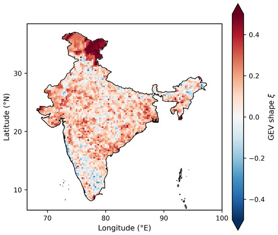
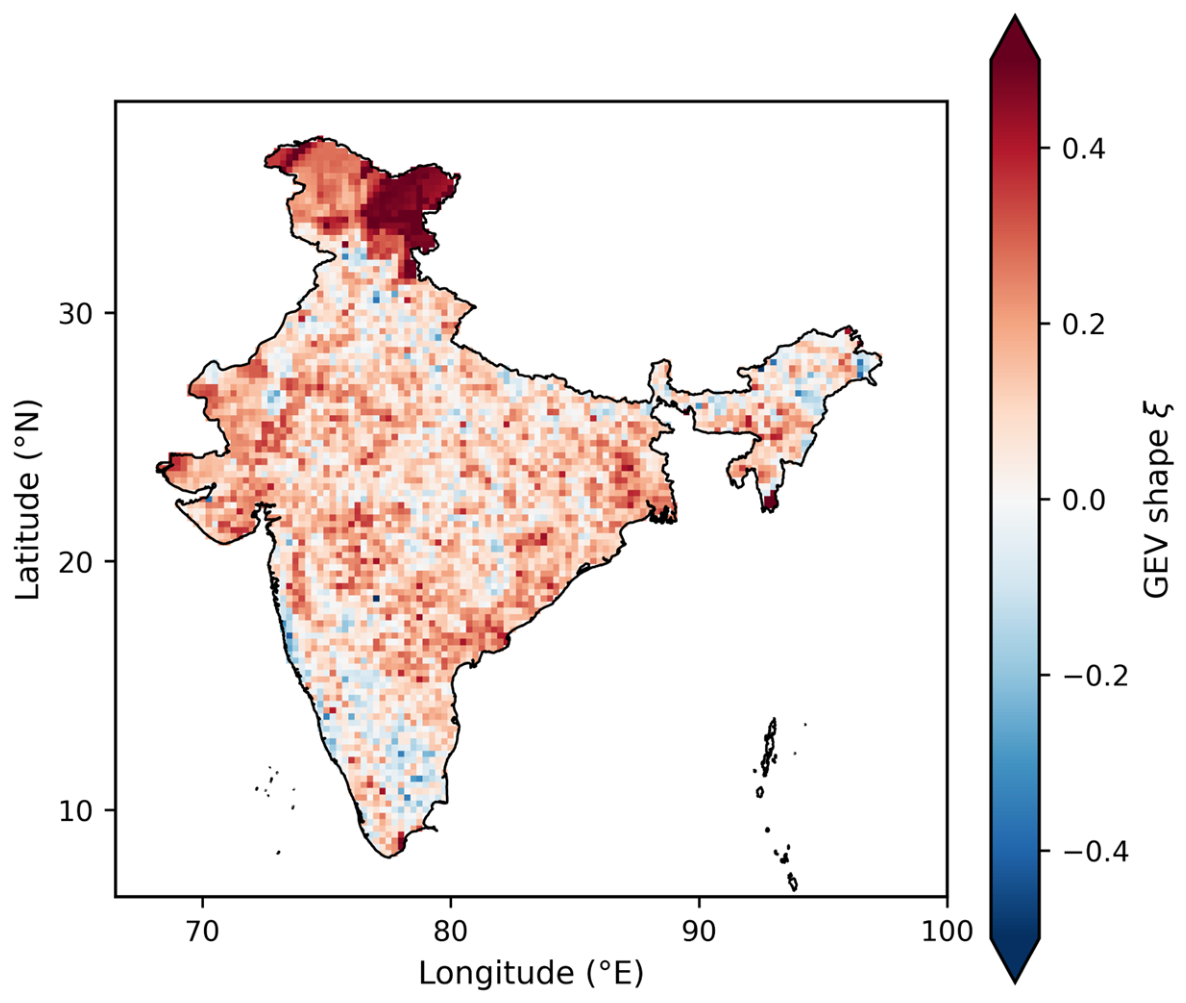
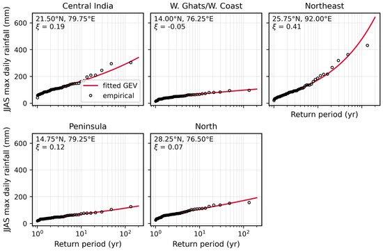
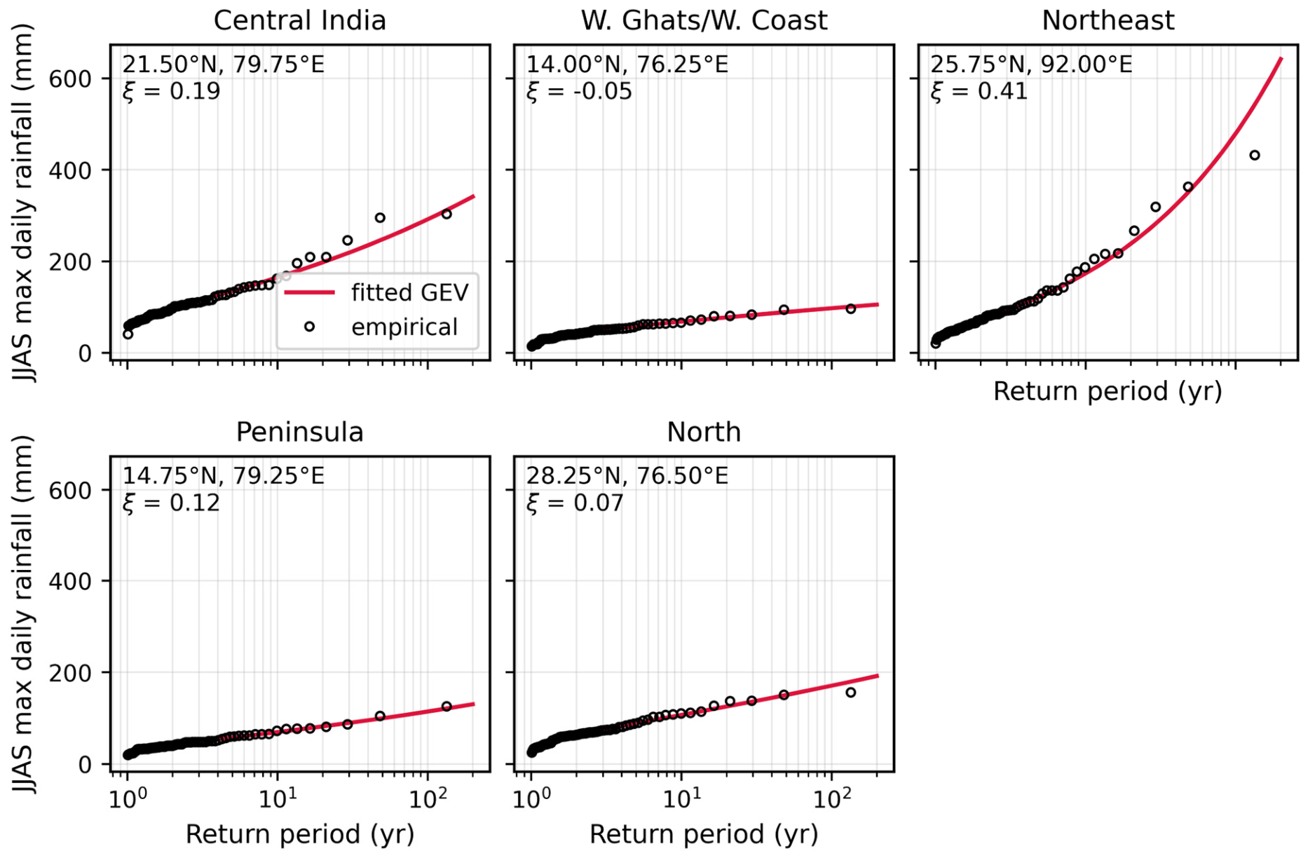
Most of the domain carries a positive GEV shape (Figure 4). The mean over the domain is ξ = 0.12 (95% CI 0.12–0.13), and 82% of cells are heavy-tailed—the regime one expects for daily rainfall over India. Elevated ξ (0.3–0.6) across the trans-Himalayan north-west is an artifact of near-zero rainfall and thin gauge coverage, not evidence of genuinely violent tails, so that strip is handled with caution throughout the paper. Diagnostic fits at a representative cell in each zone (Figure 5) confirm that the GEV hugs the empirical return levels across all five zones.
Figure 4.
Shape parameter ξ of the GEV fitted to JJAS seasonal maxima, 1951–2025.
Figure 5.
Return-level diagnostics for the GEV at one representative cell per zone (empirical Gringorten points against the fitted curve).
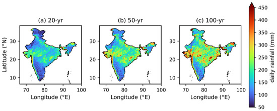
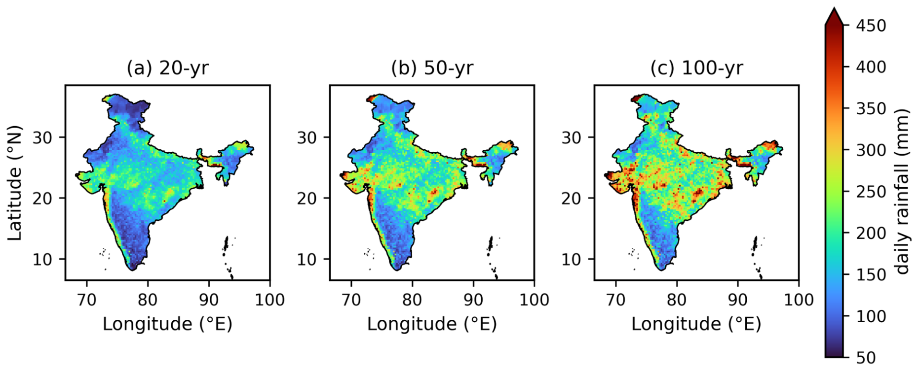
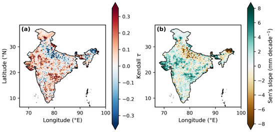
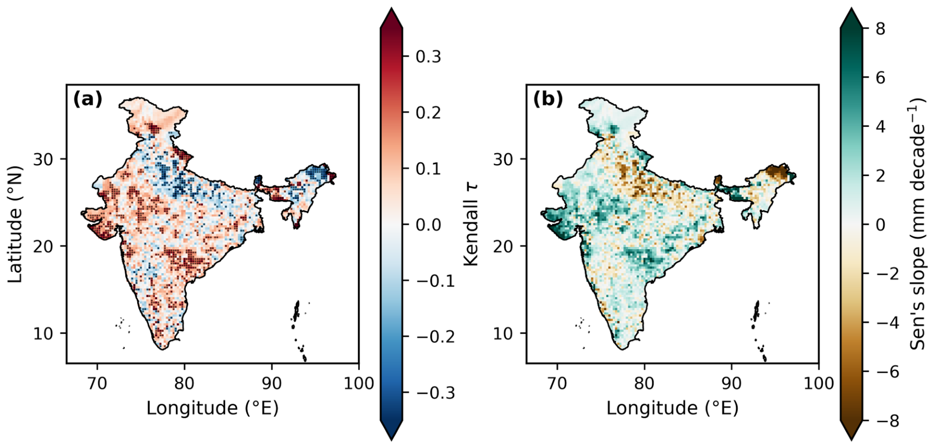
Domain-averaged return levels (Figure 6, Table 2) come to 195 mm at 50 years and 229 mm at 100 years, with the usual maxima along the Konkan coast and in the Northeastern hills. Annual JJAS maxima show significant trends at 986 of 4615 cells (21.4%)—663 upward, 314 downward and nine with a Sen slope of exactly zero (Figure 7)—and the domain-mean seasonal maximum climbs by 1.1 mm decade−1 (p = 0.0002). The increases cluster over Gujarat, along the west coast and across much of Central India; decreases appear in stretches of the Indo-Gangetic plain and in the far northeast. That geography agrees with earlier assessments [2,12].
Figure 6.
GEV return levels over 20-, 50- and 100-year return periods, plotted on a shared color scale.
Table 2.
Domain-mean and zone-wise GEV/GPD parameters and return levels. The 95% CIs come from 1000 cell-resampling bootstraps; the spatial p5/p95 columns show the spread within each region.
Figure 7.
(a) Mann–Kendall τ for the annual JJAS maxima (dots indicate p < 0.05). (b) Sen’s slope (mm decade−1).
4.2. Full-Period Extremal Dependence
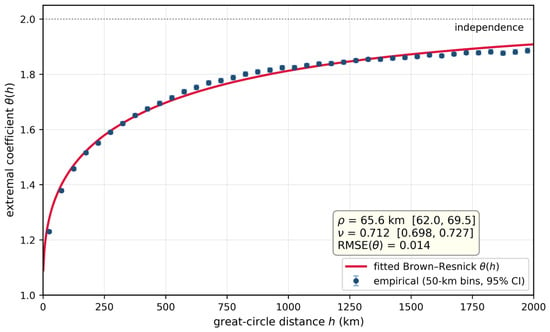
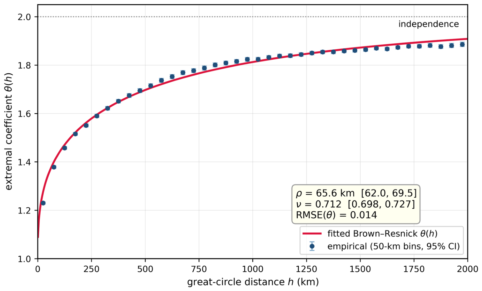
The full-period empirical θ(h) appears in Figure 8. Dependence falls off sharply within the first ~200 km and levels out towards independence beyond ~1000 km. Fitting the Brown–Resnick curve to the binned estimates gives ρ = 65.6 km (95% CI 62.0–69.5) and ν = 0.712 (0.698–0.727), with a weighted root-mean-square error (RMSE) of 0.014. At fixed separations the empirical values read θ(50 km) = 1.30, θ(100 km) = 1.42, θ(200 km) = 1.53 and θ(300 km) = 1.61—even 300 km apart, then, JJAS extremes remain well short of independence. Two features of the figure deserve a remark, and both are expected: the first bin lies a little below the fitted curve (a short-range nugget, typical of gridded rainfall), and past ~1500 km the empirical values saturate just beneath the model. Neither matters for ρ, which the short-range flank of the curve controls.
Figure 8.
Empirical extremal coefficient θ(h) for the full period (1951–2025) in 50 km bins (whiskers: 95% year-bootstrap intervals), together with the fitted Brown–Resnick curve.
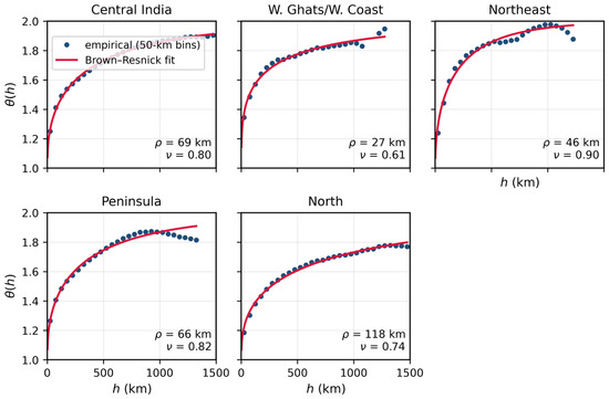
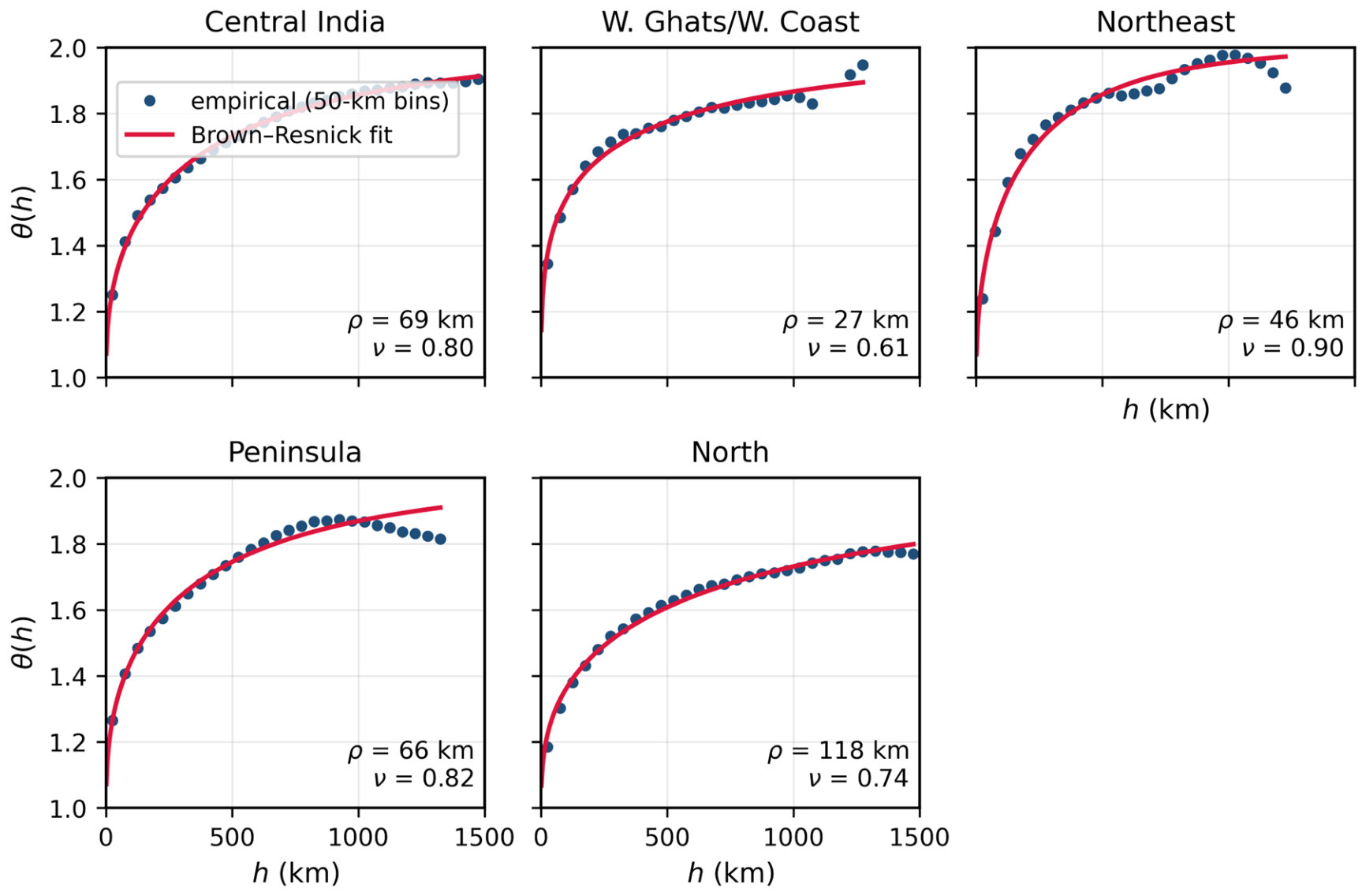
Zonal contrasts are large (Figure 9). Shortest of all is the Western Ghats/West Coast zone (ρ ≈ 27 km), where orographic rain decorrelates rapidly along the escarpment. At the other end sits the North zone (ρ ≈ 118 km): rainfall there is synoptically forced and spatially extensive, shaped by the monsoon trough and by western disturbances meeting the Himalayan foothills. Central India (ρ ≈ 69 km) and the Peninsula (ρ ≈ 66 km) occupy the middle ground, while the Northeast (ρ ≈ 46 km) loses coherence quickly in its complex terrain.
Figure 9.
θ(h) over the full period, zone by zone (points: 50 km bins from dedicated pair samples drawn within each zone; curves: Brown–Resnick fits).
4.3. Temporal Change in the Dependence Structure
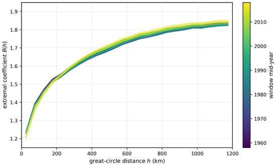
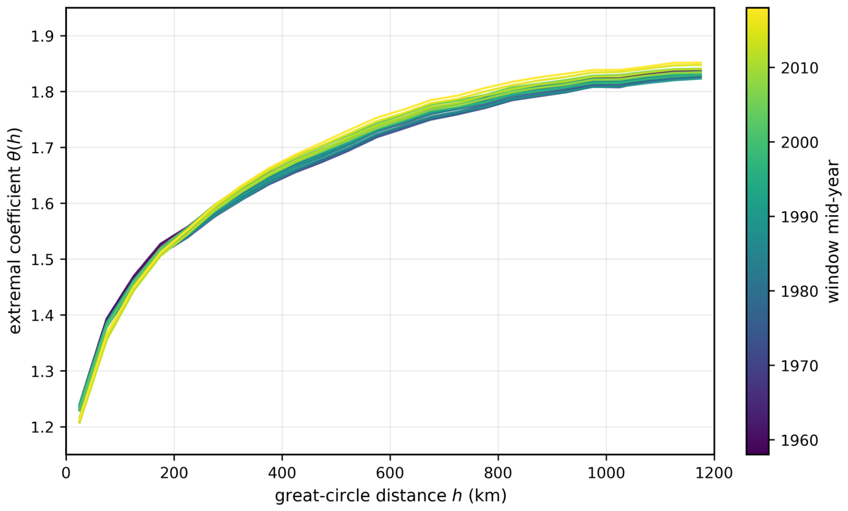
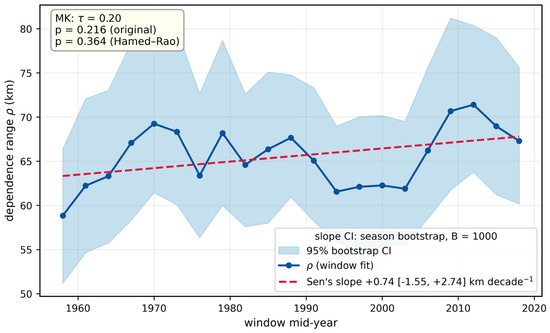
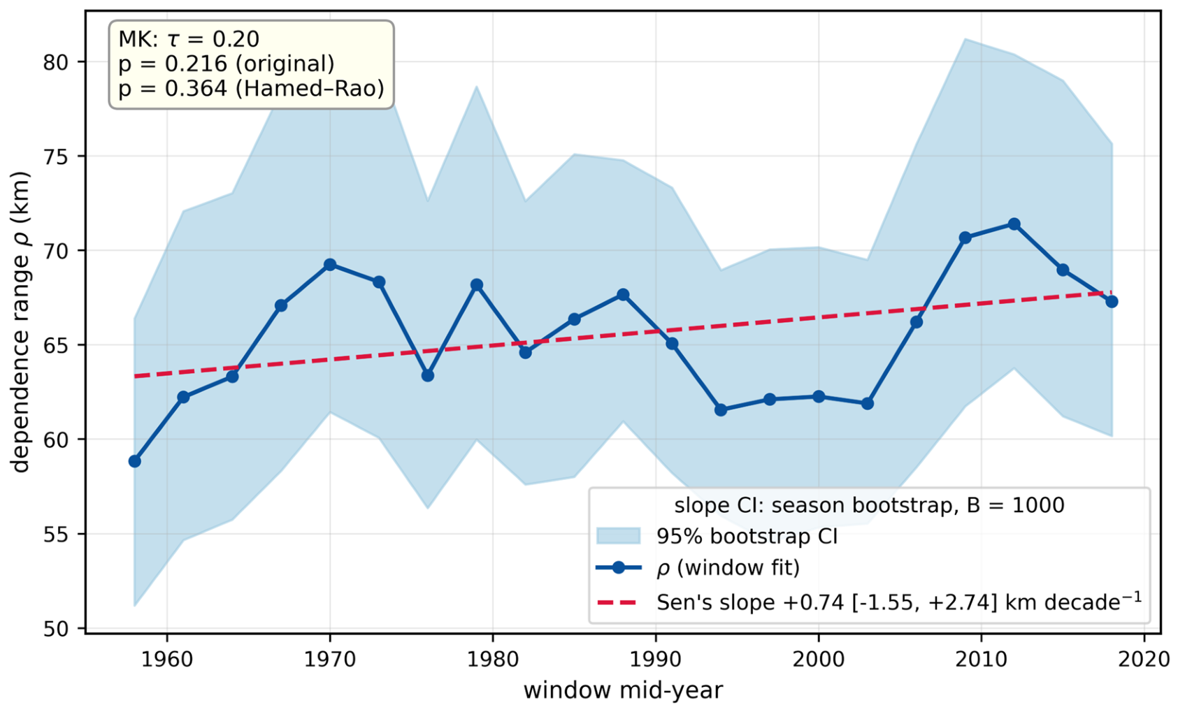
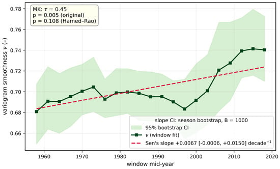
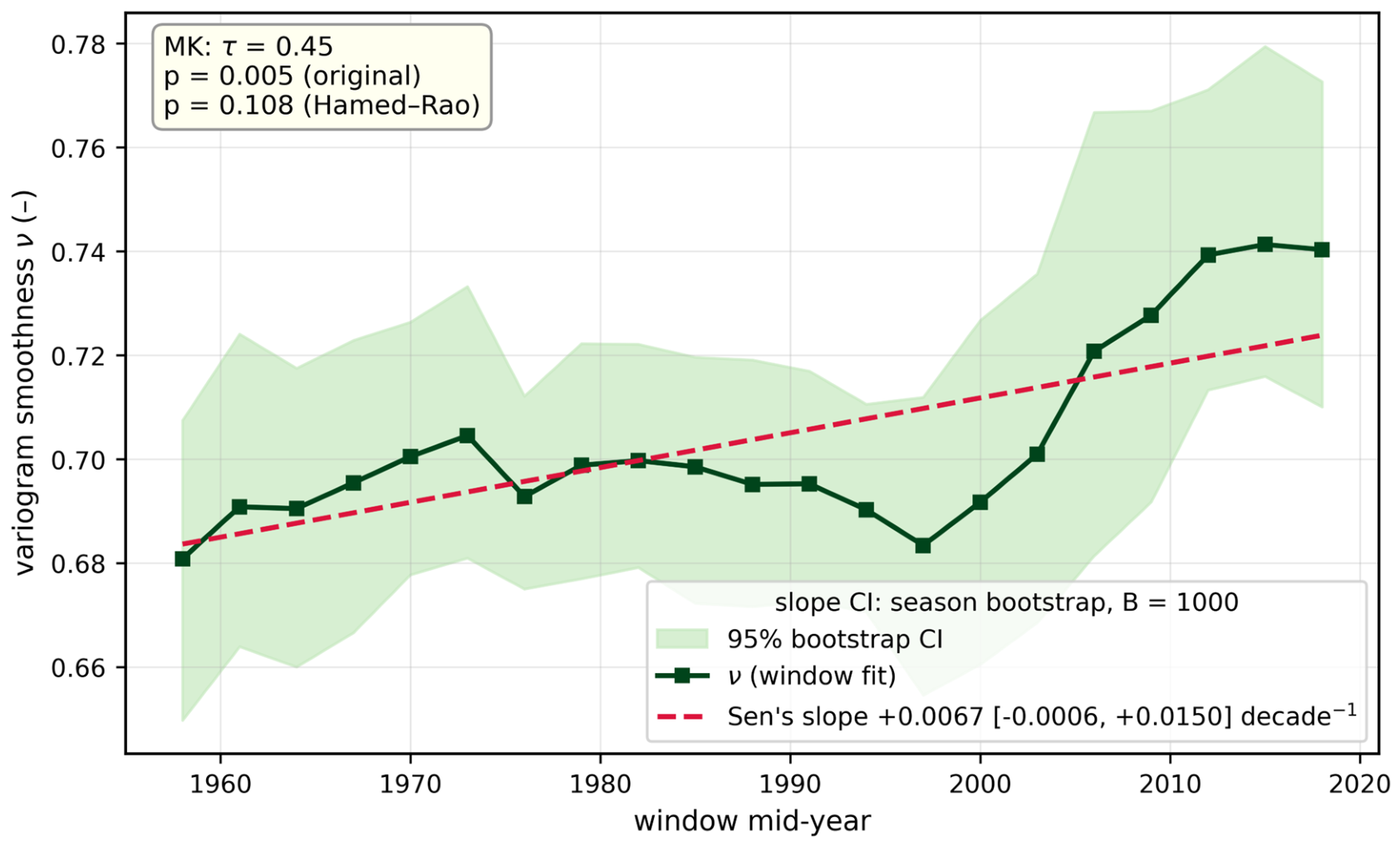
Figure 10 stacks all 21 window curves onto one set of axes. At small separations the later windows (yellow) lie noticeably beneath the earlier ones (violet): within ~200 km, extremes co-occur more strongly now than they did at the start of the record. The fitted dependence range (Figure 11, Table 3) climbs from 58.8 km in 1951–1965 to 67.3 km in 2011–2025, a Sen slope of +0.74 km decade−1. That climb does not survive scrutiny, though. Successive windows overlap by 80%, and once this is accounted for the all-India trend loses significance (τ = 0.20, original p = 0.216, Hamed–Rao p = 0.364). The smoothness parameter, meanwhile, drifts upward towards the end of the record (Figure 12), at +0.007 decade−1 (original p = 0.005, corrected p = 0.11)—a sign that the decay of dependence beyond the range has steepened. The replicate-consistent bootstrap of Section 3.4 gives a 95% interval on the all-India Sen slope of [−1.55, +2.74] km decade−1, which includes zero, and on the ν slope of [−0.001, +0.015] decade−1. Repeating the window analysis with the 0–50 km bin excluded leaves the Peninsular slope at +4.1 km decade−1 (Hamed–Rao p = 0.0002, against +4.6 km decade−1 and p < 10−4 with the bin included), the central-Indian slope at +1.6 km decade−1 (p = 0.0103, against +1.7 km decade−1 and p = 0.0171), and the all-India ρ and ν slopes (+0.65 km decade−1, p = 0.4134; +0.007 decade−1, p = 0.1131) unchanged in sign and significance; none of the twelve all-India and zonal ρ and ν series changes its verdict, and the full-period all-India range moves from 65.6 to 63.9 km.
Figure 10.
Empirical θ(h) in each 15-year window, color-coded by the window’s mid-year.
Figure 11.
All-India dependence range ρ over the 21 windows, showing the 95% bootstrap band, Sen’s slope, and the Mann–Kendall p-values before and after serial correction. The band is the marginal 95% interval of each window’s estimate; because neighboring windows share most of their seasons, it does not represent the uncertainty of the trend (Section 3.4). Legend: Sen’s slope with its replicate-consistent bootstrap 95% interval (Section 3.4).
Table 3.
All-India fitted dependence range and smoothness in each 15-year window, with 95% year-bootstrap CIs and the RMSE of the fit.
Figure 12.
The same as Figure 11, but for the variogram smoothness ν. Legend: Sen’s slope with its replicate-consistent bootstrap 95% interval (Section 3.4).
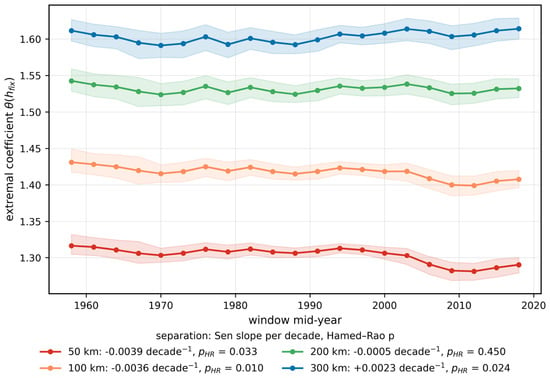
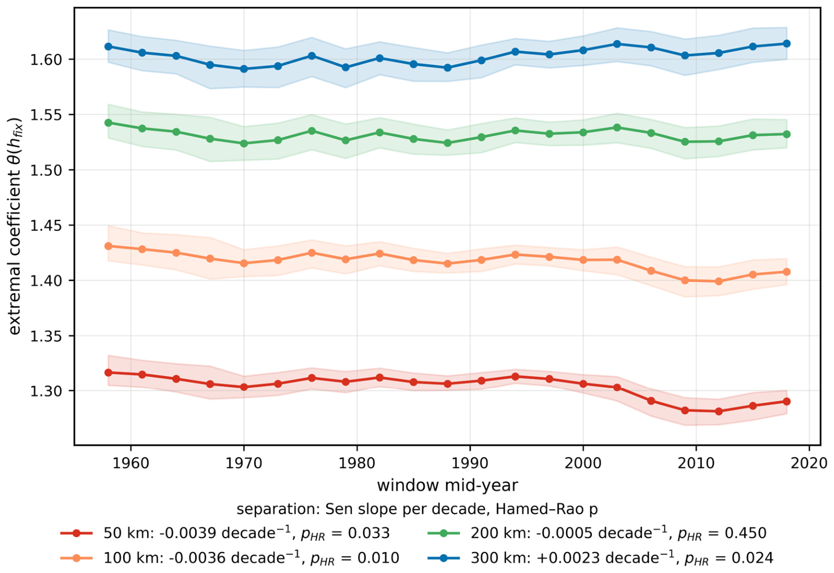
Fixing the separation makes the picture sharper (Figure 13, Table 4). θ fell at both 50 km and 100 km, at −0.004 decade−1 (Hamed–Rao p = 0.033 and 0.010 respectively; bootstrap 95% intervals [−0.0073, −0.0013] and [−0.0073, −0.0004] decade−1, both excluding zero); θ at 200 km shows no trend; θ at 300 km crept up at +0.002 decade−1 (p = 0.024; bootstrap interval [−0.0024, +0.0067] decade−1, which includes zero, so the 300 km increase is suggestive rather than resolved). Set beside the rising ν, this is not a uniform shift but a reshaping of the curve: dependence has strengthened at the mesoscale—the envelope of organized convective systems and monsoon lows—while decaying somewhat faster at sub-continental distances. Under Equation (8), this is just the signature of ρ and ν increasing together: θ falls inside the range while rising well beyond it.
Figure 13.
Extremal coefficient across the windows at fixed separations of 50, 100, 200 and 300 km (shading: 95% bootstrap CI; legend: Sen slope per decade with the corrected p).
Table 4.
Trend tests on the extremal coefficient at fixed separations (all-India, 21 windows).
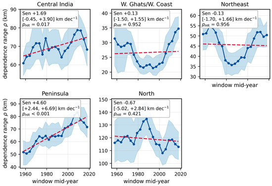
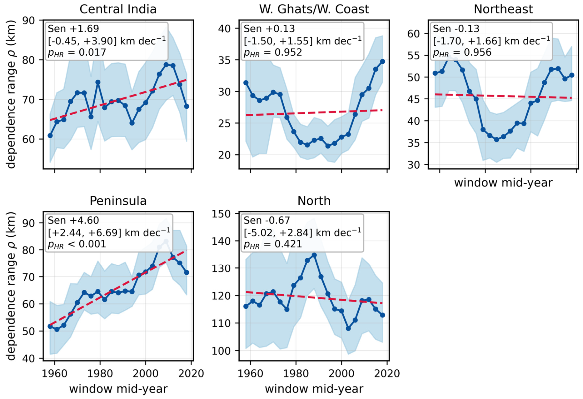
Zonal window trends (Figure 14, Table 5) pin the signal down. The Peninsula strengthens fastest, at +4.6 km decade−1 (corrected p < 10−4); Central India follows at +1.7 km decade−1 (p = 0.017). Nothing significant emerges over the Western Ghats, the Northeast or the North, though the west-coast zone describes a V-shape, shrinking into the 1980s–90s before recovering. An all-India curve averaged over such opposed regional behaviors is bound to understate the reorganization beneath it. The replicate-consistent bootstrap interval on the Peninsular slope is [+2.4, +6.7] km decade−1 and on the central-Indian slope [−0.4, +3.9] km decade−1, which includes zero.
Figure 14.
Dependence range ρ(t) for each zone, with 95% bootstrap bands and Sen’s-slope lines. Legend: Sen’s slope with its replicate-consistent bootstrap 95% interval (Section 3.4).
Table 5.
Trend tests on ρ(t) and ν(t) for all-India and each zone. Slopes are given per decade; significance is judged on the serially corrected p-value.
4.4. Regional Localisation of the Change
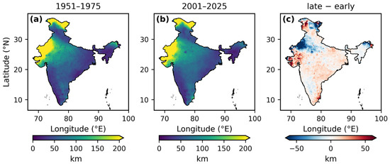
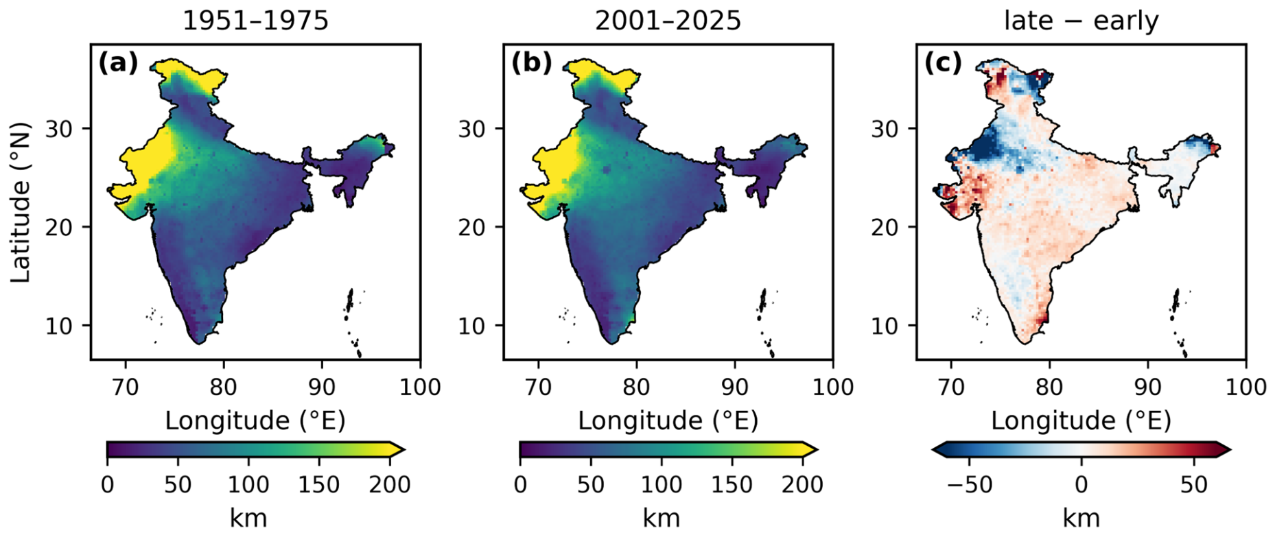
Where the block contrast is strong it is unambiguous (Figure 15, Table 6). Peninsular ρ grew from 56.3 km in 1951–1975 to 76.4 km in 2001–2025—+36%, with a paired-bootstrap 95% CI on the change of [+9.6, +30.0] km and p = 0.002. Central India moved from 66.0 to 72.5 km (+10%, p = 0.19), and all-India from 62.9 to 67.4 km (+7%, p = 0.31); neither is individually significant, and the remaining zones barely moved. On the local-ρ difference map the expansion shows up as a broad, mild reddening over the Peninsula and Central India, strongest along the southeastern coast and over Gujarat, set against pockets of contraction along the north-west Himalayan belt.
Figure 15.
Local dependence range computed from each cell’s ≤250 km neighborhood, with ν held at its full-period value: (a) 1951–1975, (b) 2001–2025, (c) late minus early.
Table 6.
Early-block (1951–1975) versus late-block (2001–2025) dependence range, with 95% bootstrap CIs and paired-bootstrap significance for the change.
4.5. Footprint of Extreme Days
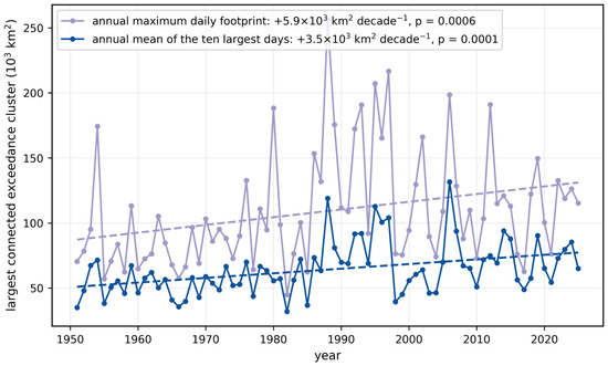
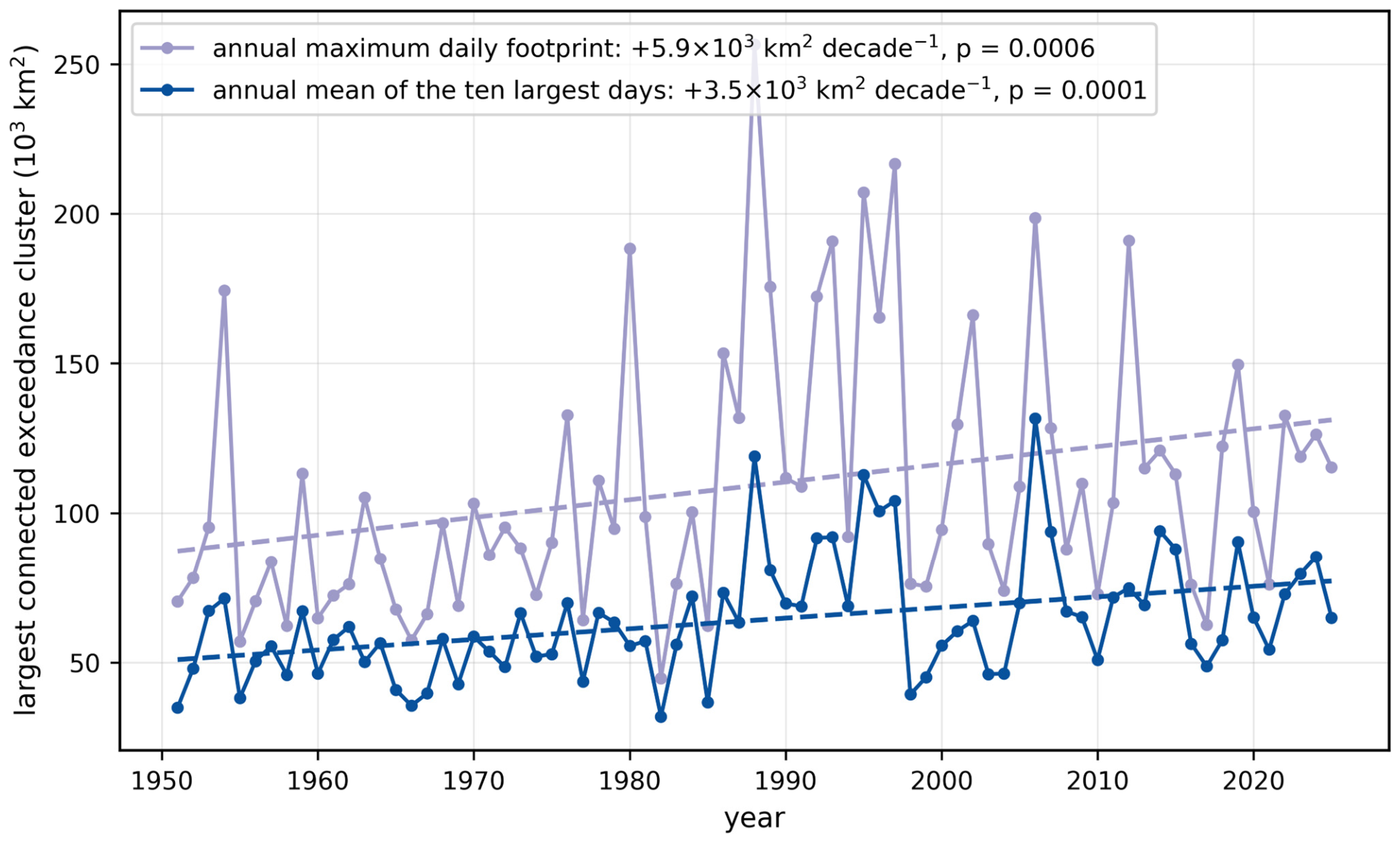
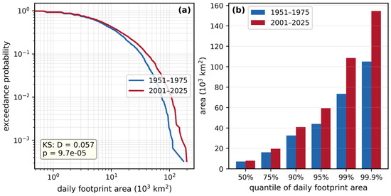
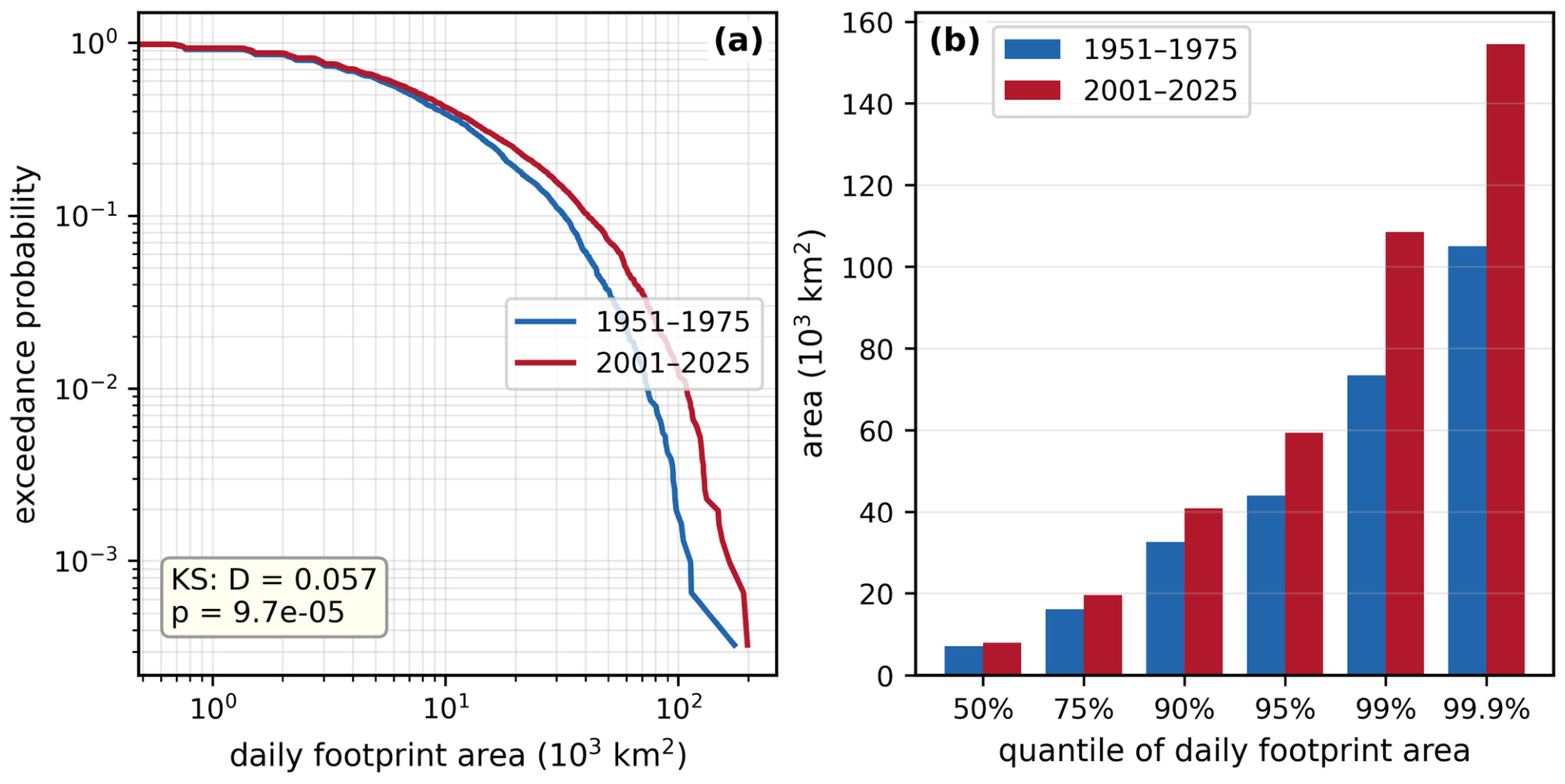
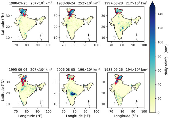
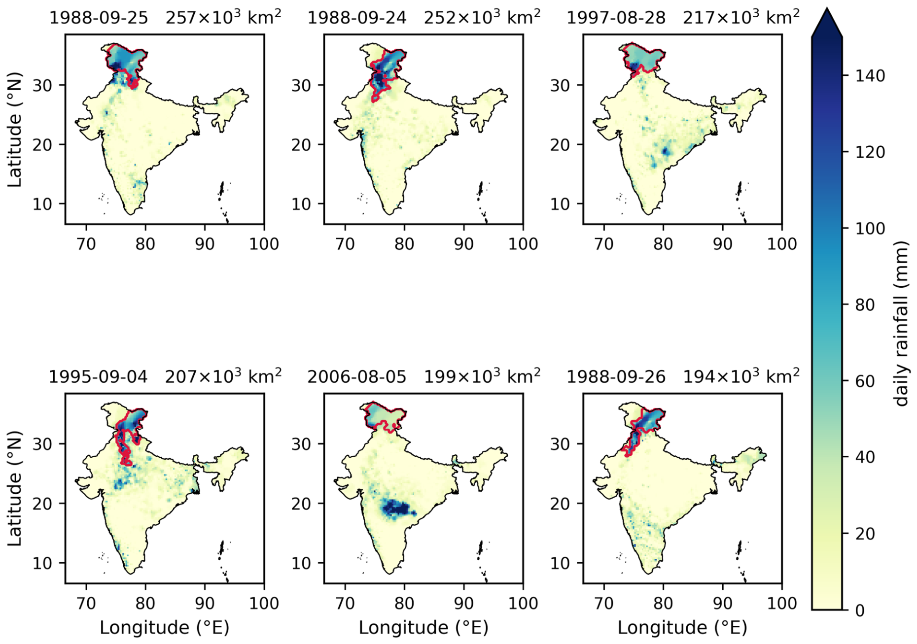
Footprint metrics provide an independent check on the dependence analysis that involves no rank transformation at all (Figure 16, Table 7). Averaged over the ten largest daily exceedance clusters each year, footprint area increased at 3536 km2 decade−1 (p = 0.0001)—roughly +41% across the 75 years—while the annual maximum rose at 5926 km2 decade−1 (p = 0.0006). Between the early and late blocks, the entire daily distribution moved (Kolmogorov–Smirnov D = 0.057, p = 9.7 × 10⁻⁵; Figure 17); the 99th percentile of daily footprint area climbed from 73 × 103 to 108 × 103 km2, a gain of +48%. The six record footprint days (Figure 18) are all organized synoptic systems—monsoon depressions and coastal lows—whose largest connected clusters cover 1.7–2.6 × 10⁵ km2. The growing joint-exceedance area shows what the θ decline at storm-scale separations looks like on the ground, and it agrees with the widespread-extremes picture that Roxy et al. [12] drew from a wholly different estimator, and it is the observed counterpart of the expansion in the area of long-duration extreme events that downscaled CMIP6 projections anticipate for the coming decades [9].
Figure 16.
Annual footprint metrics—mean of the top-10 days and annual maximum—with Sen’s-slope lines overlaid.
Table 7.
Trend tests on footprint area, together with the early-vs-late distribution comparison (KS test).
Figure 17.
Daily footprint-area distributions for the early and late blocks: (a) exceedance curves; (b) upper quantiles.
Figure 18.
The six JJAS days with the largest footprints, 1951–2025; the red contour marks the largest connected cluster of cells exceeding their local 99th percentile.
4.6. Change-Point Analysis
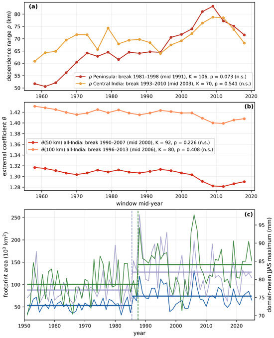
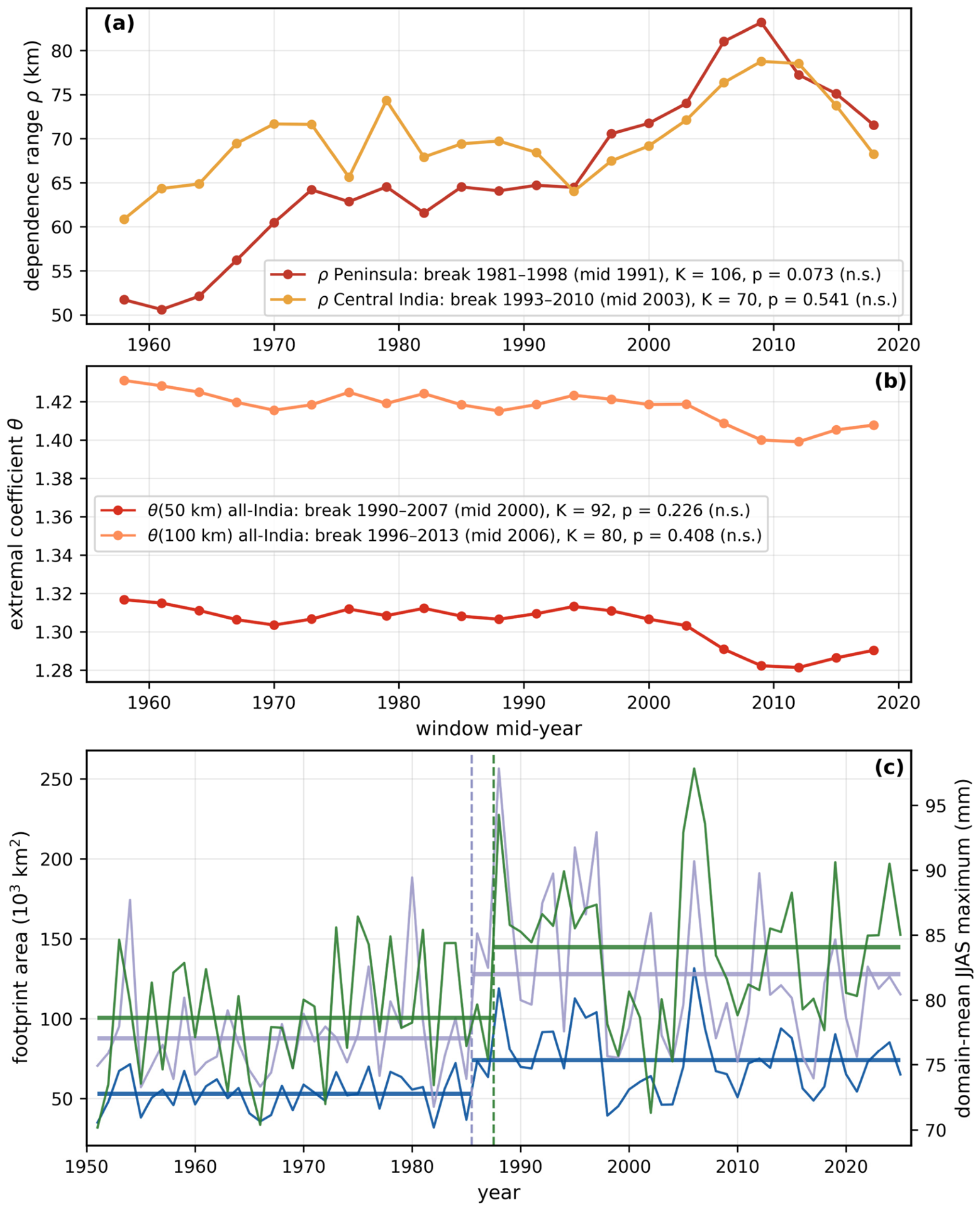
Table 8 lists the Pettitt statistics for the annual and sliding-window series, and Figure 19 marks the detected change points on the corresponding series. For the three annual series the test is unambiguous. The domain-mean JJAS maximum shifts upward between 1987 and 1988 (K = 788, p = 0.0003), its mean rising from 78.6 to 84.1 mm (+7%). Both footprint series break between 1985 and 1986: the mean of the ten largest daily footprints from 52.9×10³ to 73.8×10³ km2 (+39%; K = 856, p < 10−4) and the annual maximum footprint from 87.8 × 10³ to 127.9 × 10³ km2 (+46%; K = 828, p = 0.0001). The asymptotic values agree with a 10,000-permutation check for all three series (permutation p = 0.0003, < 10−4 and < 10−4). For the window series no break survives the permutation null. Peninsular ρ comes closest: its most probable break lies between the 1981–1995 and 1984–1998 windows (mid-year 1991), with pre- and post-break means of 59.3 and 73.4 km, but a K of 106 is reached or exceeded in 7.3% of the 2000 permutations (p = 0.0735). Central-Indian ρ (K = 70, most probable break at the 1996–2010 window, mid-year 2003, means 67.9 and 74.6 km) gives p = 0.5407; θ at 50 km (K = 92, 1993–2007, mid-year 2000, means 1.310 and 1.292) gives p = 0.2264; and θ at 100 km (K = 80, 1999–2013, mid-year 2006, means 1.421 and 1.404) gives p = 0.4078. The all-India series show no step either (ρ: K = 58, p = 0.7616; ν: K = 88, p = 0.2844). Under exchangeable seasons the 80% overlap of the windows alone produces a median K of 72 and a 95th percentile of 108 for a 21-point series, so the window design, which resolves monotonic trends (Table 5), has little power to locate a single break.
Table 8.
Pettitt change-point test on annual and sliding-window series. For the window series (n = 21) the p-value is taken from the 2000-permutation null of Section 3.6; for the annual series (n = 75) it is the asymptotic value of Equation (19).
Figure 19.
Pettitt change points. (a) Window series of the dependence range ρ(t) for the Peninsula and Central India; (b) all-India θ at 50 and 100 km; (c) the three annual series—the mean of the ten largest daily footprints and the annual maximum footprint (left axis) and the domain-mean JJAS maximum (right axis). Each legend entry gives the most probable break, K and p; vertical dashed lines and pre-/post-break means are drawn only where p < 0.05, which is the case for the annual series alone (domain-mean maximum 1987|1988, K = 788, p = 0.0003; footprints 1985|1986, K = 856 and 828, p < 10−4 and p = 0.0001). No window series has a break significant against the 2000-permutation null (Peninsular ρ: mid-year 1991, K = 106, p = 0.0735).
For the dependence series the absence of a detectable step is itself informative: the strengthening of dependence over the Peninsula and Central India is better described as a progressive trend than as an abrupt transition, and a 21-point series of overlapping windows has, in any case, little power to date a single break. The steps that are detected belong to the marginal and footprint series and fall in 1986–1988, within the period in which the Arabian Sea and the western Indian Ocean warmed rapidly and the westerly moisture supply to Central India strengthened [10,12]; they mark the point at which the area of widespread extreme days moved to a higher level, on which the gradual reorganization of dependence is superimposed. With a single realization of the climate system, however, a change point detected in a 75-season record cannot be separated from low-frequency internal variability of the monsoon, and it is presented here as a description of the record rather than as evidence of a forced regime shift.
4.7. Synthesis
Table 9 gathers every trend and change test in one place. A coherent core emerges. Extremal dependence at storm scales strengthened (θ at 50–100 km, significant); the dependence range grew precisely where the monsoon’s convective heartland sits (strongly significant over the Peninsula on every test applied, and significant for Central India in the window analysis on the serially corrected Mann–Kendall test, with a bootstrap slope interval that includes zero); extreme-day footprints expanded (significant on three separate tests); and marginal maxima intensified. Only the all-India ρ series, which averages opposing regional signals, falls short of significance. Taken alone, each of these lines of evidence could be argued away; that they all point the same way is the result. Change-point tests separate the two kinds of series: all three annual series step up in 1986–1988 (Pettitt p ≤ 0.0003), whereas none of the window series show a break that survives the season-permutation null (Table 8), so the strengthening of dependence enters this synthesis as a gradual drift on which the mid-1980s step in marginal maxima and footprints is superimposed.
Table 9.
Master synthesis of all trend and change tests; significance refers to the serially corrected p-value where one applies, and to the test’s own p-value otherwise.
5. Discussion
What emerges is a monsoon in which extreme rainfall is becoming better organized in space across the same regions where marginal intensity is rising. Three physical strands make this reading plausible. The first is the moisture-flux mechanism of Roxy et al. [12]: episodic surges of westerly moisture transport off a warming Arabian Sea moisten a broad longitudinal corridor across Central India, favoring convection that breaks out simultaneously over hundreds of kilometers. The same warming of the Arabian Sea and the western Indian Ocean has been linked to the pronounced recent wetting of north-west India [10], which is where the marginal increases in Figure 7 are concentrated. The imprint such surges would leave in θ(h)—a dependence range that stretches over the Peninsula and Central India even as the orographically anchored west-coast zone stays put—is precisely what we observe. A second strand involves monsoon low-pressure systems. These synoptic vortices structure rainfall over areas of order 105 km2, so any shift in their track density, intensity, or moisture loading feeds straight into the joint statistics of daily extremes; that our footprint growth is driven from its upper quantiles fits this reading. The third strand is the steepening smoothness ν, which tells us that extremes have become better connected at mesoscale separations while coherence at 300+ km grows no faster: the gain in organization is happening inside event envelopes, not through events merging into subcontinental monoliths.
It is instructive to set this against the marginal-only view. Trend studies of point rainfall [2,6] and covariate-based extreme-value models [24] quantify how much rain falls at a location at a fixed probability; whether neighboring points fail together is a question they cannot answer. Our rank-based estimator discards marginal information by construction, so the trends reported in Section 4.3 and Section 4.4 are additional to the documented marginal intensification, not a restatement of it. For basin-scale flood risk the two compound multiplicatively: aggregate loss models that update margins while holding spatial dependence fixed will understate the upper tail of basin-aggregated rainfall across Peninsular India. The event-synchronization literature [13,14] saw the spatial organization; what the extremal-coefficient route adds is a calibrated, model-connectable measure of it—ρ and ν are precisely what a Brown–Resnick simulator of synthetic monsoon extremes takes as input. Placing the Indian result beside the only comparable analysis elsewhere is instructive: over southern France, Maume-Deschamps et al. [25] found spatial extremal dependence weakening with time, whereas over the Peninsular and Central India it strengthens at the mesoscale. Dependence non-stationarity is therefore not of one sign globally; its direction is set by the regional dynamics—here, by the organization of monsoon convection—and must be established region by region.
6. Implications for Design and Risk Assessment
The operational content of the extremal coefficient is the pairwise joint-exceedance probability. For two sites separated by h in a max-stable field with common margins F, the probability that both exceed a level z of marginal exceedance probability p = 1 − F(z) is
to first order in p. The quantity χ(h) = 2 − θ(h) is thus the factor by which the joint risk at two sites exceeds the independent-sites value, expressed relative to p, and every change in θ reported above translates into it directly; because the daily-scale θ of Section 3.2 is a summary of rank dependence rather than a max-stable coefficient in the literal sense (Section 7), the numbers that follow are first-order indications rather than exact probabilities. For all-India, χ rose from 0.683 to 0.710 at 50 km and from 0.569 to 0.592 at 100 km between the first and last windows—increases of 3.9% (95% interval [+1.5, +6.8]%) and 4.1% ([+0.8, +8.1]%) in the probability of simultaneous exceedance at the storm scale. Over the Peninsula, where the change is largest, the block-to-block growth of ρ from 56.3 to 76.4 km at the zone’s fitted smoothness ν = 0.82 raises χ from 0.527 to 0.577 at 100 km (+9.4%, [+4.4, +14.7]%) and from 0.402 to 0.459 at 200 km (+14.2%, [+6.6, +22.7]%); read directly from the binned estimates of the two blocks, without the fitted curve, the corresponding increases are 9.5% ([+6.0, +12.9]%) and 5.4% ([+0.9, +9.8]%). The two readings agree at 100 km; at 200 km the fitted curve, which holds ν at its full-period value and so projects the growth of ρ onto larger separations, gives the larger figure, and the binned estimate is the model-free reference. These increases are additional to the marginal intensification, not a restatement of it, because the estimator is blind to the margins by construction; for basin-aggregated rainfall the two compound multiplicatively.
Four practical consequences follow. (i) Design rainfall for catchments: Areal reduction factors, which convert point design rainfall to catchment-average design rainfall in standard hydrological practice, are a direct function of the spatial dependence of extremes and are applied as fixed, stationary curves. A growing dependence range raises the areal reduction factor at any given catchment area, so basin design rainfall rises even where the point return level is unchanged; over the Peninsular and Central India, stationary depth–area relations are therefore biased low. (ii) Aggregate flood-loss and reinsurance modeling: Catastrophe models that update marginal hazard while holding a calibrated spatial correlation structure fixed will understate the upper tail of portfolio-aggregated loss, since it is precisely the joint tail that drives aggregate exceedance. (iii) Disaster-response planning: The 48% growth in the 99th percentile of daily footprint area, from 73 × 103 to 108 × 103 km2, is an operationally interpretable number: it is the area over which a single day’s response resources must be spread at a given severity, and it bears on the pre-positioning of national response assets and on multi-reservoir operation within a basin, where simultaneous inflow across sub-basins removes the buffering that staggered inflow provides. (iv) Model evaluation and stochastic simulation: ρ and ν are directly computable from any gridded output, so the θ(h) curve provides a target for testing whether CMIP6, CORDEX-South Asia or convection-permitting simulations reproduce the observed organization of monsoon extremes—a property that the standard point-wise indices do not test [8,9]—and the same two parameters are exactly what a Brown–Resnick simulator requires to generate synthetic extreme-rainfall fields for stress-testing; joint and conditional return levels of this kind are now routinely computable with available software [22].
7. Limitations
These conclusions carry five caveats. First, our treatment of dependence rests on the empirical extremal coefficient and a parametric summary θ(h); at no point do we fit a full Brown–Resnick process via pairwise likelihood, meaning ρ and ν describe the madogram curve rather than being maximum-likelihood estimates of the process itself. Second, we compute the F-madogram over all JJAS days instead of component-wise maxima. Applied at the daily scale in this way—which is standard practice—it captures the rank dependence of the full field, and the resulting θ values are best read as summaries of dependence rather than max-stable coefficients in the literal sense. Third, this is a rainfall-only analysis with no dynamical covariates, leaving the physical attribution in Section 5 circumstantial and resting on mechanisms documented in the published literature. Fourth, the IMD gridded product inherits a rain-gauge network that thins towards the Himalaya and the Northeast and has not stayed constant through time; where gauges are sparse, interpolation smooths the field and can locally exaggerate apparent spatial coherence [32,33,34]. Results for the North and Northeast zone, the trans-Himalayan strip above all, deserve corresponding caution—though the strongest signals in this study come from the Peninsula and Central India, where gauge coverage is at its densest and most stable. Four features of the design bear on whether a changing network could have manufactured the trends. The estimator acts on rank-transformed fields, so it is invariant to any monotone, time-invariant distortion introduced by interpolation; only a change in the smoothing operator itself could alias into ρ(t). Excluding the shortest distance bin, where smoothing acts most strongly, changes none of the twelve all-India and zonal ρ and ν trend verdicts and moves the Peninsular slope only from +4.6 to +4.1 km decade−1 (Section 4.3). The footprint diagnostic involves no rank transformation and no parametric dependence model, yet returns the same direction of change on three independent tests. And the significant signals are located where gauge coverage is densest and most stable, while the zones with the weakest and least stable coverage show no significant change—the opposite of what a network-density artifact would produce. Cross-validation of ρ against the station-based ensemble product for India [32], whose 30-year record is too short to test the trend but can bound the interpolation contribution to the full-period estimate, is a natural next step. Fifth, the five zones are administrative aggregates rather than statistically homogeneous regions, so data-driven regionalizations of the extremal dependence structure [23] could sharpen the zonal contrasts; and a change point detected in a single 75-season realization cannot be separated from low-frequency internal variability of the monsoon (Section 4.6).
8. Conclusions
Working from 75 monsoon seasons of 0.25° gridded rainfall, we draw six conclusions. (1) The characteristic range of all-India extremal dependence for JJAS daily extremes is 66 km (62–70 km). (2) θ at 50 and 100 km fell significantly over 21 sliding windows (corrected p ≤ 0.03), while ρ climbed from 59 to 67 km, although the all-India ρ trend itself does not survive serial-correlation correction. (3) The change is regional rather than uniform: the dependence range over Peninsular India grew by 36% between 1951–1975 and 2001–2025 (p = 0.002); the central Indian window trend is significant on the serially corrected Mann–Kendall test, though its bootstrap slope interval includes zero, whereas the West Coast, Northeast, and North show no change. (4) The largest connected daily exceedance cluster expanded in area by ~40% (p ≤ 0.0006), and its 99th percentile rose 48% between blocks. (5) Marginal maxima intensified over the same period (+1.1 mm decade−1 in the domain mean). (6) A Pettitt change-point analysis finds no abrupt shift in the dependence series: the Peninsular strengthening is a progressive trend whose most probable break, about 1991, is not significant against a permutation null that respects the window overlap (p = 0.0735), whereas the domain-mean JJAS maximum stepped up in 1988 and the annual footprint series in 1986 (p ≤ 0.0003). Indian monsoon rainfall extremes, therefore, do not possess a stationary spatial dependence structure, and this reorganization compounds the well-documented marginal intensification rather than simply accompanying it. In practical terms, the joint probability of simultaneous extreme rainfall at sites 100–200 km apart over Peninsular India has risen by roughly 9% at 100 km—and by between 5% and 14% at 200 km, depending on whether the change is read from the binned estimates or from the fitted curve—within the observational record, independently of the rise in point return levels; design depth–area relations, aggregate flood-loss models and the evaluation of climate-model output should treat the spatial dependence of monsoon extremes as a changing quantity rather than a fixed one.
Author Contributions
Conceptualization, N.L., S.K., F.F.B.H. and M.Z.; methodology, N.L. and S.K.; software, N.L.; formal analysis, N.L.; investigation, N.L. and M.Z.; data curation, N.L.; resources; F.F.B.H. and M.Z.; writing—original draft preparation, N.L.; writing—review and editing, S.K., F.F.B.H. and M.Z.; visualization, N.L.; supervision, S.K. and M.Z.; project administration, M.Z. All authors have read and agreed to the published version of the manuscript.
Funding
This research was funded by Princess Nourah bint Abdulrahman University Researchers Supporting Project number (PNURSP2026R675), Princess Nourah bint Abdulrahman University, Riyadh, Saudi Arabia.
Institutional Review Board Statement
Not applicable.
Informed Consent Statement
Not applicable.
Data Availability Statement
The IMD 0.25° gridded daily rainfall product [26] is distributed by the India Meteorological Department, Pune (https://www.imdpune.gov.in). India national and state boundary shapefiles were used for masking and zonation. The derived arrays, figures, tables and the complete analysis code, including the fixed random seeds used for every bootstrap, are available from the corresponding author on reasonable request; every number reported here can be regenerated from the archived scripts.
Acknowledgments
The authors extend their appreciation to Princess Nourah bint Abdulrahman University Researchers Supporting Project number (PNURSP2026R675), Princess Nourah bint Abdulrahman University, Riyadh, Saudi Arabia. The authors thank the India Meteorological Department, Pune, for developing and maintaining the long-period gridded rainfall dataset on which this study rests.
Conflicts of Interest
The authors declare no conflicts of interest.
Abbreviations
The following abbreviations are used in this manuscript:
| IMD | India Meteorological Department |
| JJAS | June–September (the summer monsoon season) |
| GEV | Generalized extreme-value distribution |
| GPD | Generalized Pareto distribution |
| POT | Peaks over threshold |
| CDF | Cumulative distribution function |
| CI | Confidence interval |
| RMSE | Root-mean-square error |
| MK | Mann–Kendall |
| KS | Kolmogorov–Smirnov |
References
- Guhathakurta, P.; Rajeevan, M. Trends in the rainfall pattern over India. Int. J. Climatol. 2008, 28, 1453–1469. [Google Scholar] [CrossRef] [Scilit]
- Goswami, B.N.; Venugopal, V.; Sengupta, D.; Madhusoodanan, M.S.; Xavier, P.K. Increasing trend of extreme rain events over India in a warming environment. Science 2006, 314, 1442–1445. [Google Scholar] [CrossRef] [Scilit] [PubMed]
- Rajeevan, M.; Bhate, J.; Jaswal, A.K. Analysis of variability and trends of extreme rainfall events over India using 104 years of gridded daily rainfall data. Geophys. Res. Lett. 2008, 35, L18707. [Google Scholar] [CrossRef] [Scilit]
- Falga, R.; Wang, C. The rise of Indian summer monsoon precipitation extremes and its correlation with long-term changes of climate and anthropogenic factors. Sci. Rep. 2022, 12, 11985. [Google Scholar] [CrossRef] [Scilit] [PubMed]
- Vinnarasi, R.; Dhanya, C.T. Changing characteristics of extreme wet and dry spells of Indian monsoon rainfall. J. Geophys. Res. Atmos. 2016, 121, 2146–2160. [Google Scholar] [CrossRef] [Scilit]
- Mukherjee, S.; Aadhar, S.; Stone, D.; Mishra, V. Increase in extreme precipitation events under anthropogenic warming in India. Weather Clim. Extrem. 2018, 20, 45–53. [Google Scholar] [CrossRef] [Scilit]
- Varikoden, H.; Reji, M.J.K. A meta-analysis of the regional extreme rainfall events in the Indian sub-continent during the southwest monsoon period. Sci. Total Environ. 2025, 977, 179339. [Google Scholar] [CrossRef] [Scilit] [PubMed]
- Varghese, S.J.; Pentakota, S.; Thadivalasa, P.; Podapati, G.; Ashok, K. Changes in physical characteristics of extreme rainfall events during the Indian summer monsoon based on downscaled and bias-corrected CMIP6 models. Sci. Rep. 2025, 15, 3679. [Google Scholar] [CrossRef] [Scilit] [PubMed]
- Konda, G.; Chowdary, J.S.; Gnanaseelan, C.; Vissa, N.K.; Parekh, A. Temporal and spatial aggregation of rainfall extremes over India under anthropogenic warming. Sci. Rep. 2024, 14, 12538. [Google Scholar] [CrossRef] [Scilit] [PubMed]
- Joseph, L.; Skliris, N.; Dey, D.; Marsh, R.; Hirschi, J. Increased summer monsoon rainfall over Northwest India caused by Hadley cell expansion and Indian Ocean warming. Geophys. Res. Lett. 2024, 51, e2024GL108829. [Google Scholar] [CrossRef] [Scilit]
- Subrahmanyam, K.V.; Kumar, P.; Nelli, N.R.; Anoop, S.; Ramana, M.V.; Rajeevan, M.; Chauhan, P. Regional shift in the peak time of maximum Indian summer monsoon rainfall in recent decades. Geophys. Res. Lett. 2025, 52, e2024GL112697. [Google Scholar] [CrossRef] [Scilit]
- Roxy, M.K.; Ghosh, S.; Pathak, A.; Athulya, R.; Mujumdar, M.; Murtugudde, R.; Terray, P.; Rajeevan, M. A threefold rise in widespread extreme rain events over central India. Nat. Commun. 2017, 8, 708. [Google Scholar] [CrossRef] [Scilit] [PubMed]
- Malik, N.; Bookhagen, B.; Marwan, N.; Kurths, J. Analysis of spatial and temporal extreme monsoonal rainfall over South Asia using complex networks. Clim. Dyn. 2011, 39, 971–987. [Google Scholar] [CrossRef] [Scilit]
- Boers, N.; Goswami, B.; Rheinwalt, A.; Bookhagen, B.; Hoskins, B.; Kurths, J. Complex networks reveal global pattern of extreme-rainfall teleconnections. Nature 2019, 566, 373–377. [Google Scholar] [CrossRef] [Scilit] [PubMed]
- Smith, R.L. Max-Stable Processes and Spatial Extremes; Unpublished manuscript; University of North Carolina: Chapel Hill, NC, USA, 1990. [Google Scholar]
- Schlather, M. Models for stationary max-stable random fields. Extremes 2002, 5, 33–44. [Google Scholar] [CrossRef] [Scilit]
- Kabluchko, Z.; Schlather, M.; de Haan, L. Stationary max-stable fields associated to negative definite functions. Ann. Probab. 2009, 37, 2042–2065. [Google Scholar] [CrossRef] [Scilit]
- Davison, A.C.; Padoan, S.A.; Ribatet, M. Statistical modeling of spatial extremes. Stat. Sci. 2012, 27, 161–186. [Google Scholar] [CrossRef] [Scilit]
- Schlather, M.; Tawn, J.A. A dependence measure for multivariate and spatial extreme values: Properties and inference. Biometrika 2003, 90, 139–156. [Google Scholar] [CrossRef] [Scilit]
- Cooley, D.; Naveau, P.; Poncet, P. Variograms for spatial max-stable random fields. In Dependence in Probability and Statistics; Bertail, P., Soulier, P., Doukhan, P., Eds.; Lecture Notes in Statistics 187; Springer: New York, NY, USA, 2006; pp. 373–390. [Google Scholar]
- Naveau, P.; Guillou, A.; Cooley, D.; Diebolt, J. Modelling pairwise dependence of maxima in space. Biometrika 2009, 96, 1–17. [Google Scholar] [CrossRef] [Scilit]
- Beranger, B.; Padoan, S.A. Modeling extremal dependence in multivariate and spatial problems: A practical perspective. Extremes, 2026; in press. [CrossRef] [Scilit]
- Maume-Deschamps, V.; Ribereau, P.; Zeidan, M. Regionalization of the extremal dependence structure using spectral clustering. Stoch. Environ. Res. Risk Assess. 2025, 39, 725–745. [Google Scholar] [CrossRef] [Scilit]
- Athira, K.; Singh, S.; Abebe, A. Rising risk and localized patterns of Indian summer monsoon rainfall extremes. Atmos. Res. 2024, 309, 107554. [Google Scholar] [CrossRef] [Scilit]
- Maume-Deschamps, V.; Ribereau, P.; Zeidan, M. A spatio-temporal model for temporal evolution of spatial extremal dependence. Spat. Stat. 2024, 64, 100860. [Google Scholar] [CrossRef] [Scilit]
- Pai, D.S.; Sridhar, L.; Rajeevan, M.; Sreejith, O.P.; Satbhai, N.S.; Mukhopadhyay, B. Development of a new high spatial resolution (0.25° × 0.25°) long period (1901–2010) daily gridded rainfall data set over India and its comparison with existing data sets over the region. MAUSAM 2014, 65, 1–18. [Google Scholar] [CrossRef] [Scilit]
- Mann, H.B. Nonparametric tests against trend. Econometrica 1945, 13, 245–259. [Google Scholar] [CrossRef] [Scilit]
- Kendall, M.G. Rank Correlation Methods, 4th ed.; Griffin: London, UK, 1975. [Google Scholar]
- Sen, P.K. Estimates of the regression coefficient based on Kendall’s tau. J. Am. Stat. Assoc. 1968, 63, 1379–1389. [Google Scholar] [CrossRef]
- Hamed, K.H.; Rao, A.R. A modified Mann–Kendall trend test for autocorrelated data. J. Hydrol. 1998, 204, 182–196. [Google Scholar] [CrossRef] [Scilit]
- Pettitt, A.N. A non-parametric approach to the change-point problem. J. R. Stat. Soc. Ser. C Appl. Stat. 1979, 28, 126–135. [Google Scholar] [CrossRef] [Scilit] [PubMed]
- Peringiyil, A.; Saharia, M.; Sreejith, O.P.; Wood, A.W.; Mohapatra, M.; Sabde, B.; Kumari, A.; Phadkar, B.; Sabeerali, C.T.; Rohini, P.; et al. A station-based 0.1-degree daily gridded ensemble precipitation dataset for India. Sci. Data 2025, 12, 333. [Google Scholar] [CrossRef] [Scilit] [PubMed]
- Goteti, G.; Famiglietti, J. Extent of gross underestimation of precipitation in India. Hydrol. Earth Syst. Sci. 2024, 28, 3435–3455. [Google Scholar] [CrossRef] [Scilit]
- Jena, P.; Garg, S.; Azad, S. Performance analysis of IMD high-resolution gridded rainfall (0.25° × 0.25°) and satellite estimates for detecting cloudburst events over the Northwest Himalayas. J. Hydrometeorol. 2020, 21, 1549–1569. [Google Scholar] [CrossRef] [Scilit]
- Coles, S. An Introduction to Statistical Modeling of Extreme Values; Springer: London, UK, 2001. [Google Scholar]

Disclaimer/Publisher’s Note: The statements, opinions and data contained in all publications are solely those of the individual author(s) and contributor(s) and not of MDPI and/or the editor(s). MDPI and/or the editor(s) disclaim responsibility for any injury to people or property resulting from any ideas, methods, instructions or products referred to in the content. |
© 2026 by the authors. Licensee MDPI, Basel, Switzerland. This article is an open access article distributed under the terms and conditions of the Creative Commons Attribution (CC BY) license.