


Abstract
This study investigated future changes in extreme climate events over China under carbon neutrality using an improved reliability ensemble averaging (REA) method, based on 12 Coupled Model Intercomparison Project Phase 6 (CMIP6) models under the SSP1-1.9 and SSP1-2.6 scenarios. Results indicated that carbon neutrality is reached in 2042/2063 under SSP1-1.9/SSP1-2.6. Relative to 1995–2014, the areal-mean increases in annual mean temperature (Tav), hottest day temperature (TXx), coldest night temperature (TNn), total precipitation (Prcptot), and heavy precipitation (R95p) are 1.27/1.61 °C, 1.31/1.69 °C, 1.45/1.84 °C, 9.5/13.3%, and 20.8/29.6% under SSP1-1.9/SSP1-2.6, respectively. Larger increases in Tav and TNn occur in northeastern (NE) and northern China, while those in TXx occur in northwestern (NW) China. Temperature projections are most (least) robust in southeastern China (NE). Prcptot increases largely in the Tibetan Plateau (TB) and NE, while R95p increases largely in TB and south of the Yangtze River. The smallest but most robust precipitation increase is in southwestern China, while the least robust is in NW. The areal-mean Tav, TXx, and TNn increase by 0.34 °C, 0.38 °C, and 0.39 °C under SSP1-2.6 (late carbon neutrality) compared with SSP1-1.9 (early carbon neutrality), while those for Prcptot and R95p increase by 3.8% and 8.8%, respectively. Achieving carbon neutrality earlier may contribute to mitigating future climate change and reducing the worsening of extreme temperature and precipitation extremes over parts of China.
1. Introduction
The Sixth Assessment Report (AR6) of the Intergovernmental Panel on Climate Change (IPCC) clearly shows that global mean surface temperature (GMST) in 2010–2019 is 1.07 °C (0.8–1.3 °C) higher than pre-industrial, and greenhouse gases are the main cause of global warming, contributing 1.0–2.0 °C of warming [1,2,3]. Climate extremes have changed dramatically across the planet, including decreases in extreme cold events, increases in heat waves and droughts, as well as changes in frequency, severity and duration of extreme precipitation events [4,5,6,7]. To address the increasingly severe challenge of climate change, the international community has adopted the Paris Climate Agreement of 2015. It aims to limit the increase in GMST, relative to pre-industrial levels, to well below 2.0 °C and proposes a more ambitious target of 1.5 °C by the end of this century [8]. In this context, China, as a major carbon emitter, proposed the “dual carbon” goals in September 2020, aiming to peak carbon emissions by 2030 and achieve carbon neutrality by 2060.
China is located in the East Asian monsoon region and has complex terrain and diverse climate conditions. While experiencing rapid economic and social development, it also faces great pressure to reduce carbon emissions. With the intensification of global warming, China has experienced an increase in extreme climate events over recent decades, causing colossal losses to natural ecosystems and human society. For example, since 1990, extreme meteorological disasters have caused annual GDP losses of 2.37% in China [9]. Therefore, reliable projections of mean and extreme climate changes in China are of great scientific significance and practical value for climate adaptation.
With the proposal of the “dual carbon” goals, many studies have focused on regional climate changes in China under carbon neutrality [10,11,12,13,14,15,16]. The recent development in Global Climate Models (GCMs) from Coupled Model Intercomparison Project phase 6 (CMIP6) provides a reliable data foundation for these studies. The sustainable development Shared Socioeconomic Pathways (SSP1-1.9 and SSP1-2.6) in CMIP6 provide feasible pathways for achieving global temperature control targets, consistent with China’s “dual carbon” goals, and can be used to assess potential climate impacts under such targets [17,18,19]. Against the backdrop of China achieving the “dual carbon” goals, global warming by the end of this century could be reduced by approximately 0.16–0.21 °C [10]. Deng et al. found that, compared with the historical reference period, annual mean temperature in China is projected to increase by 1.22 °C and 1.58 °C under the SSP1-1.9 and SSP1-2.6 scenarios, and mean annual precipitation is projected to increase by 7.1% and 9.9%, respectively. These increases are much smaller than those under the non-carbon-neutral SSP2-4.5 scenario, especially in Northwest China [11]. Extreme climate changes under carbon neutrality are also significantly different from those under scenarios without carbon neutrality. Compared with the SSP5-8.5 scenario, extreme warm events over the Tibetan Plateau are greatly reduced under the SSP1-2.6 scenario during the carbon neutrality period. Increases in extreme heavy precipitation and maximum consecutive dry days are also markedly reduced in some regions of China [14]. Relative to the 1995–2014 baseline, the Ganjiang River Basin would have more abundant water resources and lower-intensity extreme hydrological events under the “dual carbon” pathways [15]. The increase in intensity of compound hot-dry events in the Yangtze River Delta is significantly reduced under SSP1-1.9 [16]. It is worth noting that, under the SSP1-1.9 scenario, global mean warming is projected to overshoot 1.5 °C and then return to 1.5 °C by the end of this century; however, the frequency and intensity of climate extremes do not return to pre-1.5 °C levels [20]. Thus, whether carbon neutrality is achieved, and how early it is achieved, has significant impacts on climate change in China, particularly for climate extremes.
The above-mentioned studies on carbon neutrality across China have been based on previous GCMs. Although climate models have developed rapidly, and the latest CMIP6 models have been greatly improved in model design, resolution, and physical processes compared with their previous generations [17,19]. However, considerable uncertainty remains in climate projections [7,21]. The equal-weight multi-model ensemble mean (MME) is the most commonly used method to reduce uncertainty [6,22,23,24]. However, model performance varies across regions, so simple arithmetic averaging is no longer the most reliable strategy. Therefore, various weighting methods based on model performance have been developed in recent years [25,26,27,28,29,30,31,32]. The reliability ensemble averaging (REA) method, which considers both historical performance and future convergence, is one of the most advanced weighting schemes. It was first proposed by Giorgi et al. in 2002 [29], but the original convergence criterion artificially reduced model spread and may have spuriously reduced projection uncertainty [31]. Xu et al. [31] modified this method by removing the convergence criterion and incorporating multi-variable and multi-statistic considerations. On this basis, we further improved the REA method by combining model simulation capabilities for both observed climatology and temporal variability (interannual variability), and established that this strategy performed best for climate indices in China, with the smallest biases [32]. However, existing studies applying the REA method have mostly focused on climate changes under medium and high emission scenarios, with insufficient consideration of extreme climate responses under carbon neutrality.
In summary, studies on the impacts of carbon neutrality on future climate changes in China are increasing, but most studies still use simple arithmetic ensemble means and do not introduce weighting schemes that reflect model simulation capabilities to reduce projection uncertainty. To address this gap, this study uses CMIP6 outputs and applies the improved REA method proposed in the recent work by Zhu et al. [32] to examine the regional climate changes in China under carbon neutrality. The projections of climate extremes over different regions of China under carbon neutrality are investigated, and the differences between early and late carbon neutrality are compared. This work aims to provide a scientific basis for understanding extreme climate changes under China’s “dual carbon” policy and for the formulation of adaptation strategies.
2. Data and Methods
2.1. Observations and Model Datasets
Considering the carbon neutrality targets and data availability, this study employed a number of climate datasets such as daily mean, maximum, and minimum temperature and precipitation data from 12 CMIP6 models (https://esgf-node.llnl.gov/projects/esgf-llnl, accessed on 1 September 2026, Table A1). The historical simulation (1850–2014) and two Shared Socioeconomic Pathways under low-emission scenarios (SSP1-1.9 and SSP1-2.6, 2015–2100) were used for all 12 models. The SSP1-1.9 and SSP1-2.6 experiments represent pathways of sustainable practices development, and their radiative forcing reaches 1.9 W m−2 and 2.6 W m−2 in 2100 [18]. Only one realization of each model was analyzed to allow equity and fairness among models. To determine the timing of carbon neutrality, annual atmospheric CO2 mass data (unit: kg) from CMIP6 models for 2015–2100 were also used. It should be noted that the models providing CO2 data differ from those providing temperature and precipitation data; details are given in Table A2. The observational dataset used is CN05.1, a high-resolution (0.25° × 0.25°) daily gridded dataset, which was provided by the National Climate Center of the China Meteorological Administration, and elaborated with data from 2416 observation stations across China [33]. It covers the period from 1961 to the most recent day.
2.2. Climate Indices
Six climate indices were used in this work, including the annual mean temperature (Tav), the annual total precipitation (Prcptot), and four extreme indices defined by the Expert Team on Climate Change Detection and Indices (http://etccdi.pacificclimate.org/, accessed on 1 September 2026, shown in Table 1) [34]. The annual hottest day temperature (TXx) and coldest night temperature (TNn) represent extreme high and low temperatures, respectively. The annual total precipitation for events exceeding the 95th percentile (R95p) represents intense precipitation events, and the maximum consecutive dry days (CDD) represents the dry part of the precipitation spectrum. The 95th percentile threshold for R95p is calculated based on wet days (RR ≥ 1 mm) in the historical period (1961–1990), and is computed individually for each model and for the observations. These indices have been widely used in climate change studies globally [11,17,18,19,32,34]. Prcptot and R95p were expressed as percentage changes relative to the historical reference period.
Table 1.
The definition of climate indices used in this study.
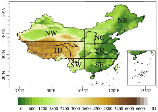
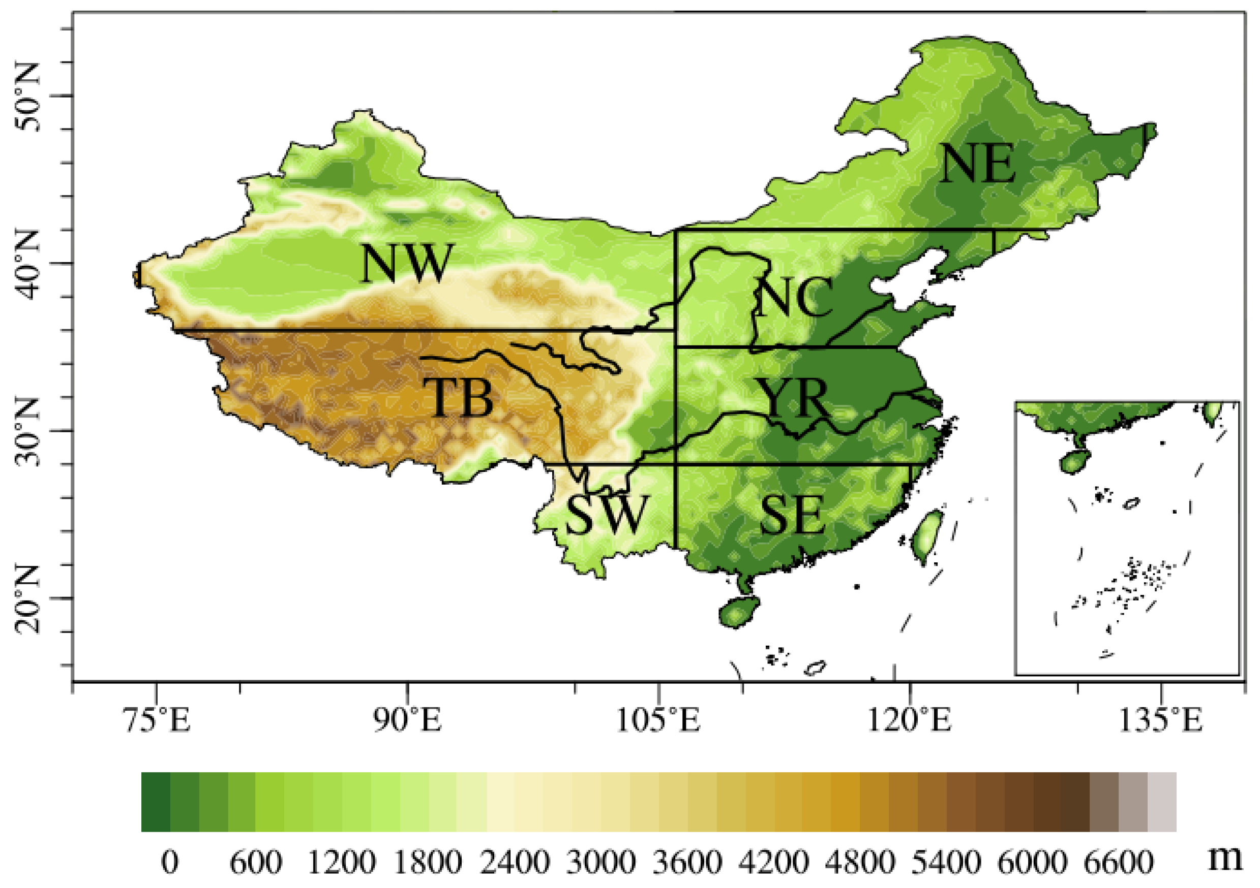
All climate indices from different models and observations were first calculated on their native grids. To facilitate the intercomparison, all results were interpolated to a common 1° × 1° grid using bilinear interpolation. To quantitatively study regional characteristics, we divided China into seven subregions based on topography and controlling climate systems, following previous studies [7]. The seven subregions are northwestern China (NW, 36°–50° N, 74°–106° E), the Tibetan Plateau (TB, 28°–36° N, 78°–106° E), southwestern China (SW, 20°–28° N, 95°–106° E), northeastern China (NE, 42°–55° N, 106°–134° E), northern China (NC, 35°–42° N, 106°–126° E), the mid-lower Yangtze River regions (YR, 28°–35° N, 106°–123° E) and southeastern China (SE, 18°–28° N, 106°–120° E) (Figure 1). Note that, in the subsequent calculations, the spatial averages for different indices over China and its subregions are all computed using latitude cosine weighting.
Figure 1.
Domains and topography (shading, units: m) of seven subregions in China.
2.3. Determination of the Carbon Neutrality Period
Following the IPCC AR6, carbon neutrality is the condition in which anthropogenic CO2 emissions associated with a subject are balanced by anthropogenic CO2 removals [1]. Carbon neutrality and net zero CO2 emissions are overlapping concepts. At the global scale, carbon neutrality and net zero CO2 emissions are equivalent [1]. Therefore, the timing of carbon neutrality can be determined from two perspectives: achieving net zero anthropogenic CO2 emissions and reaching a peak in atmospheric CO2 concentrations [11]. According to the design of the SSP scenarios, the SSP1-1.9 and SSP1-2.6 scenarios can achieve carbon neutrality by the middle of the 21st century [18]. Therefore, the SSP1-1.9 and SSP1-2.6 scenarios are selected as the carbon neutrality scenarios. Specifically, the SSP1-1.9 and SSP1-2.6 simulations used here are the standard ScenarioMIP concentration-driven runs, in which atmospheric CO2 concentration is prescribed and identical across models. This design ensures that differences among models and between scenarios reflect the climate response to the same imposed CO2 pathway, rather than differences in each model’s internally simulated carbon cycle. Considering the limited availability of CO2 emission data, the model data in Table A2 are used to identify the time when carbon neutrality is reached under the two scenarios based on the peak time of CO2 mass. Taking this year as the center, a 20-year period is defined as the carbon neutrality period in this study, consisting of 9 years before and 10 years after that year.
This study uses the multi-model ensemble to project changes in extreme indices over China during the global carbon neutrality period under the SSP1-1.9 and SSP1-2.6 scenarios relative to the historical reference period (1995–2014). Meanwhile, the differences in changes between the two carbon neutrality scenarios are compared to assess climate response differences between early and late carbon neutrality. Thus, it should be noted that the difference between early and late carbon neutrality in this study involves both temporal differences and emission scenario differences (in CO2 mass).
2.4. Reliability Ensemble Averaging Method
This study used the improved reliability ensemble averaging (REA) method [7,32], and its reliability factor Ri can be expressed as:
where the function f1 measures the model performance in reproducing the observed climatological state. The functions f2 and f3 measure the model performance in reproducing the observed temporal (interannual) variability in terms of absolute and relative deviation, respectively. The latter is a “symmetric” statistic, ensuring that two models would have the same performance measure if their model-over-observation ratio and observation-over-model ratio are equal [7]. T represents a climate variable (an extreme index in this study). Tbias is the climatological bias between the simulation and observation. Tabs,var and Trel,var are the absolute and relative bias in interannual variability between the simulation and observation. εT and εSTD are measures of the natural variability of climate indices. εT is computed as the difference between the maximum and minimum values of the 20-year moving average of the detrended observations of a variable during the historical period (1961–2014). The interannual variability of climate indices is represented by the temporal standard deviation (STD). εSTD is the difference between the maximum and minimum of the interannual variability computed for each 20-year period of a variable during the historical period (1961–2014). Tm and To are the simulated and observed climatologies. STDm and STDo are the simulated and observed interannual variability, and abs denotes the absolute value. The values of f1, f2, and f3 range from 0 to 1 (an upper limit of 1). The value of the function f1/f2 is set to 1 when abs(Tm − To)/abs(STDm − STDo) is smaller than εT/εSTD. In other words, a climate model is considered to be reliable if its bias is within the observed interannual variability. The parameters m1, m2, and m3 in Equation (1) can be used to adjust each criterion. We set them to 1 in this research.
Once the reliability factor Ri for each model has been calculated, the weight of each model (Wᵢ) is determined by the following equation:
where N is the number of models (here it is 12), Rᵢ is the reliability factor of model i, and Wᵢ is the weight of model i. Wᵢ is in fact the normalized value of Rᵢ (the weights of all 12 models sum to 1).
The weights are calculated separately for each index at each grid cell over China. In other words, the weight of each model differs across indices and grid cells. Once the weight of each model is determined, the simulated results for each index can be obtained by weighted ensemble.
Historical simulations, along with observations, are divided into a calibration period of 1961–1994 (34 years) and a validation period of 1995–2014 (20 years). The validation period also serves as the reference for future projection, following the guidelines from the previous AR6 report [1]. Once the calibration and validation are accomplished, the REA method is subsequently applied to future climate projections under the global carbon neutrality target.
2.5. Signal-to-Noise Ratio
The signal-to-noise ratio (SNR) was used to quantitatively measure the robustness of the projections [7]. The SNR for the REA method can be calculated as follows:
where ΔTi denotes the ith individual model simulated changes (under SSP1-1.9, SSP1-2.6, and their differences), and Wi is its weight. The signal (S) is the absolute value of REA. The noise (N) is the model spread, measured by the inter-model standard deviation (SD), and it is used in subsequent analyses (Section 3.3). SNR > 1 implies the signal is greater than the noise; hence, the projection is robust to a certain extent. The larger the SNR is, the greater the confidence level becomes.
3. Results
3.1. Simulation of Current Climate
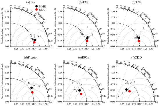
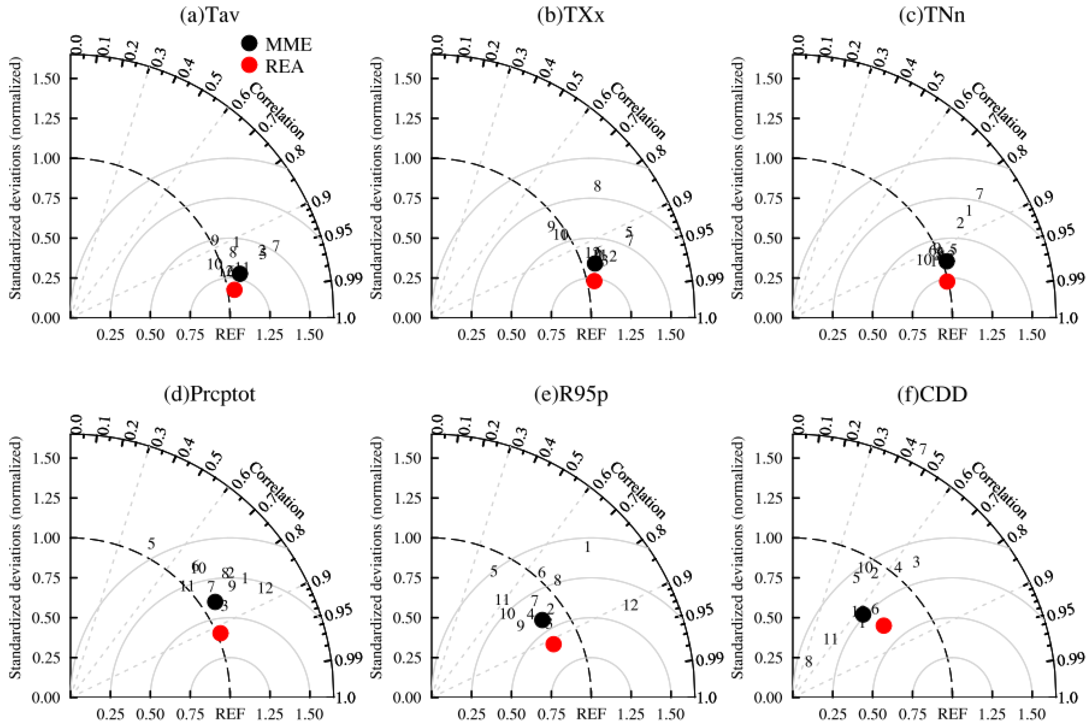
Taylor diagrams are used to evaluate the ability of 12 CMIP6 models, their multi-model ensemble mean (MME), and the REA in reproducing the spatial pattern of climate indices over China (Figure 2). The Taylor diagram provides a concise statistical summary of the degree of correlation (PCC; pattern correlation coefficient), centered root mean square error (CRMSE), and the ratio of spatial standard deviation (RSD) [21,35]. Better performance is indicated by PCC and RSD closer to 1, and smaller CRMSE. Results show that there are significant differences in the simulation capability among models, and the simulation of temperature indices is better than that of precipitation indices (Table S1). The majority of models have PCC greater than 0.85 for Tav, TXx, and TNn, while precipitation indices range from 0.45 to 0.9. This indicates that models have good performance in simulating the spatial structure of these temperature indices, with RSD from 0.89 to 1.39 and the CRMSE less than 0.5. For Prcptot and R95p, PCC ranges from 0.46 to 0.92, and the CRMSE is larger than 0.5. Models show relatively poor performance for CDD, with PCC below 0.8 and RSD far from 1. MME is clearly superior to individual models, with larger PCC and smaller CRMSE for all indices. The REA method shows improvements compared to MME, with PCC above 0.92 for all indices (except CDD), CRMSE between 0.23 and 0.57, and RSD between 0.83 and 1.05.
Figure 2.
Taylor diagram of climate indices in China during 1995–2014 simulated by CMIP6 models. Numbers indicate CMIP6 models listed in Table A1. The solid circles represent MME (black) and REA (red).
To measure the capability of models in simulating the temporal variation, we use the interannual variability skill score (IVS), as employed in Zhu et al. [21]. It can quantify the similarity of interannual variability between simulated and observed indices. STDm and STDo are the simulated and observed interannual standard variability, respectively. IVS is first calculated at each grid point and then regionally averaged. A smaller IVS indicates better performance of the simulation. Results show that the simulation of temperature indices is better than that of precipitation indices. The mean IVS is less than 1 for almost all models in temperature indices, while it is greater than 1 for precipitation indices (Table S1). For CDD, the mean IVS of MIROC-ES2L is even 6.42. For all indices, the mean IVS from REA is lower than that from MME. This indicates that the REA method outperforms MME in simulating the temporal variability of all indices.
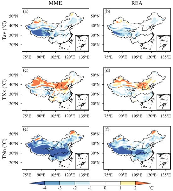
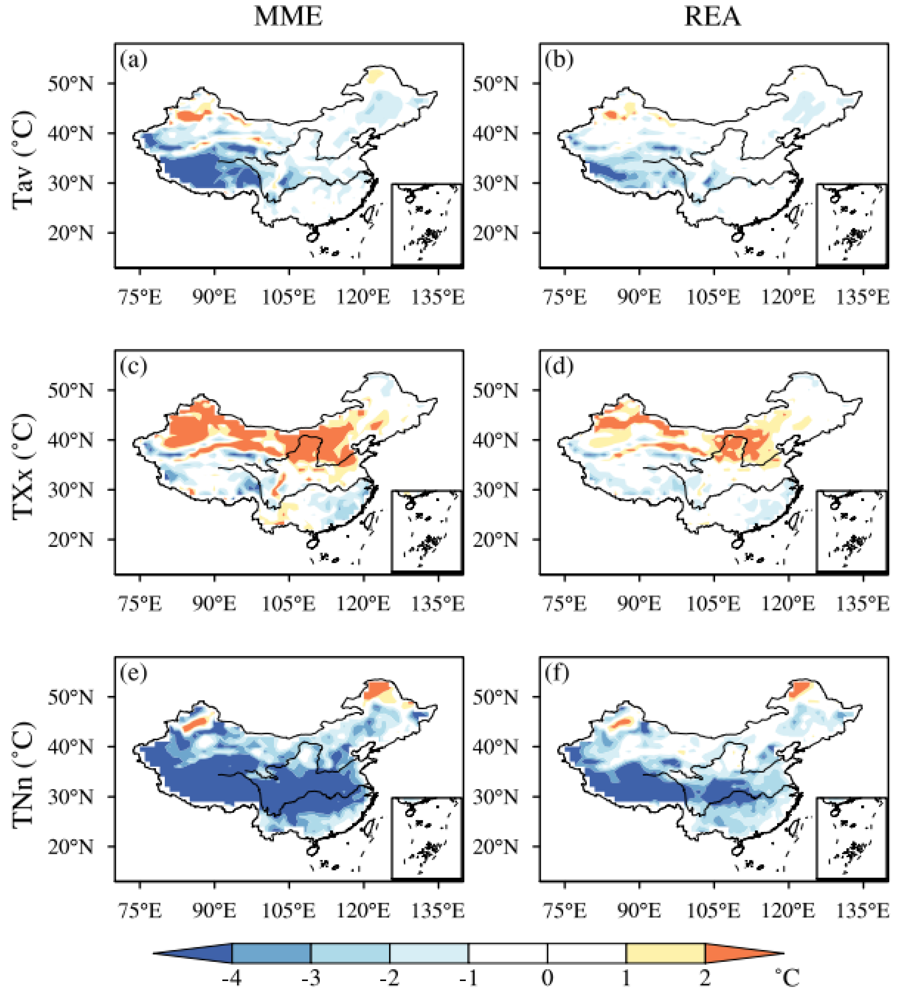
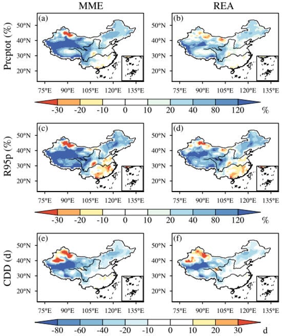
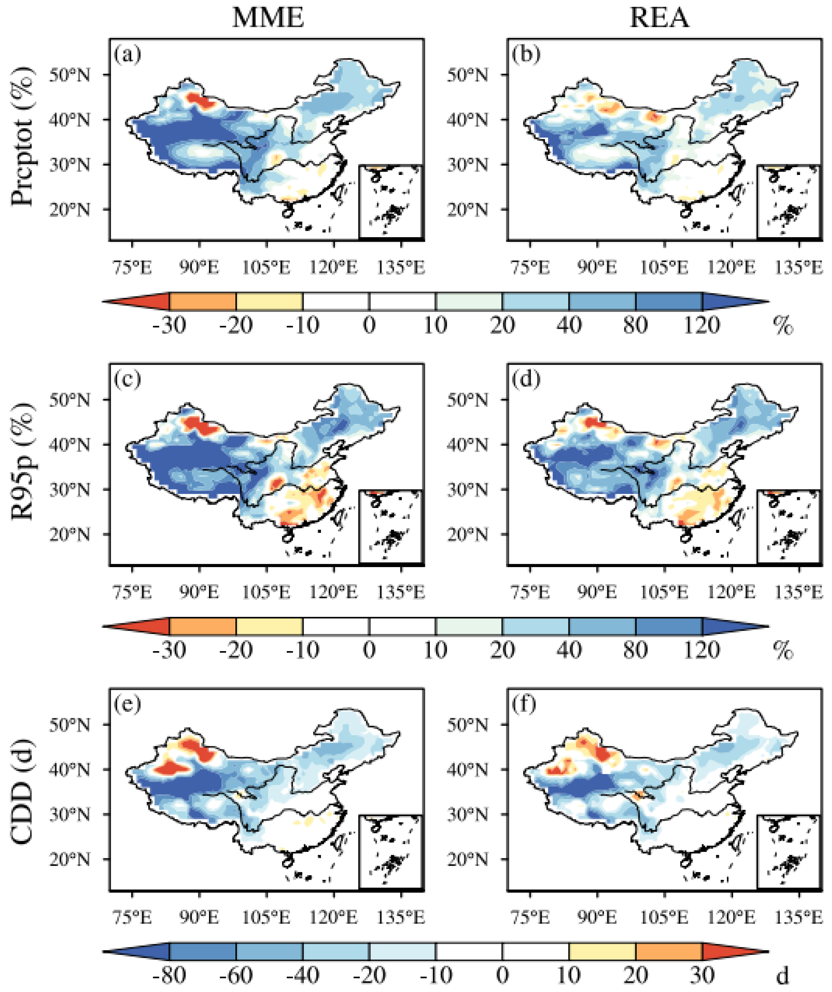
To further compare the simulation performance differences between REA and MME, Figure 3 and Figure 4 show the spatial distributions of biases between simulations (REA and MME) and observations from 1995 to 2014. The results show that MME has general cold biases for Tav and TNn throughout the country, while REA substantially reduces these cold biases. Due to topographic effects, simulation biases in northwestern (NW) China and the Tibetan Plateau (TB) regions are much larger than those in other regions (Table S2). The largest cold biases occur over TB, where the local areal-mean bias for TNn is 9.31 °C by MME, but 5.08 °C by REA (Figure 3). For TXx, MME shows negative biases over southern China and positive biases over northern China and Xinjiang, while REA slightly reduces these biases. MME generally overestimates total and heavy precipitation over China, while REA reduces these positive biases to about half of those in MME. Specifically, the areal-mean relative biases over China in MME for Prcptot and R95p are 77.4% and 94.2%, while in REA, they are 34.1% and 49.8%, respectively. The spatial distributions of biases for CDD are generally consistent between the two schemes, with positive biases in northern Xinjiang and negative biases over the north of the Yangtze River (Figure 4).
Figure 3.
The spatial pattern of biases (simulation minus observation) in MME (a,c,e) and REA (b,d,f) of temperature indices for 1995–2014. From top to bottom are Tav (a,b), TXx (c,d), and TNn (e,f), respectively.
Figure 4.
The spatial pattern of biases (simulation minus observation) in MME (a,c,e) and REA (b,d,f) of precipitation indices for 1995–2014. From top to bottom are Prcptot (a,b), R95p (c,d), and CDD (e,f), respectively.
Overall, REA performs better than MME for both the climatological pattern and the interannual variation for climate indices over China. Therefore, the REA method is used for the projections during the carbon neutrality period in the following analysis.
3.2. Global Carbon Neutrality Period
Following the IPCC AR6, carbon neutrality is a state where anthropogenic CO2 emissions associated with a subject are balanced by anthropogenic removals [1]. The report also notes that CO2 concentrations will only begin to decline after anthropogenic CO2 emissions reach net zero, meaning that the time when CO2 concentrations peak is essentially consistent with the time when anthropogenic CO2 emissions reach net zero. Therefore, given the limited CO2 data available from CMIP6 models, we use the atmospheric CO2 mass output by CMIP6 models and determine the time when global carbon neutrality is reached under different scenarios by the time when CO2 mass peaks.
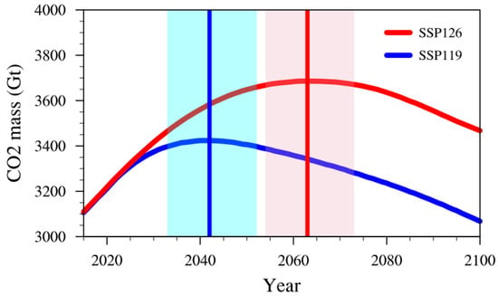
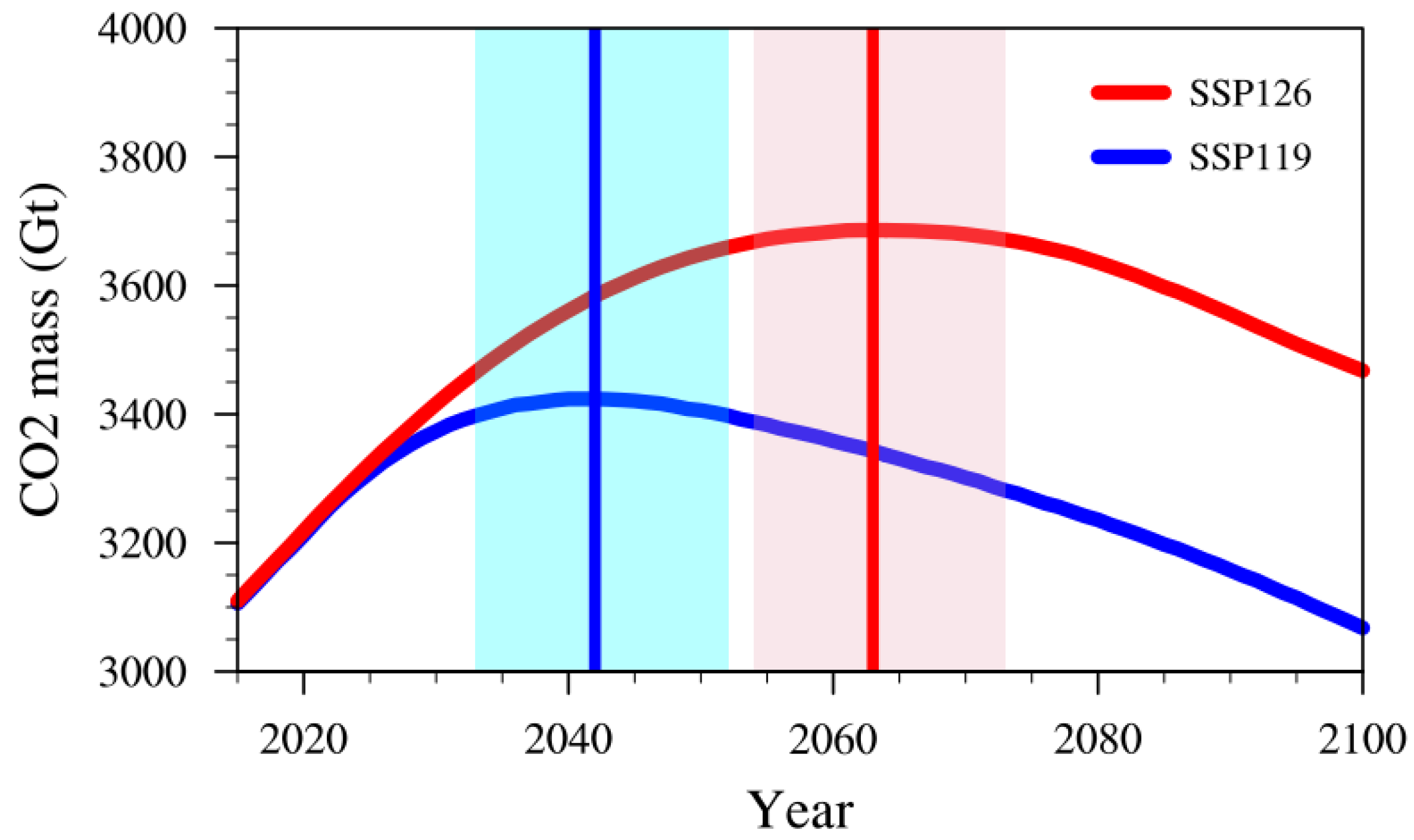
Figure 5 presents the temporal variation in atmospheric CO2 mass from MME under the SSP1-1.9 and SSP1-2.6 scenarios. Under the condition that CO2 mass reaches its peak, global carbon neutrality time is reached in 2042 under SSP1-1.9 and in 2063 under SSP1-2.6. Under both scenarios, the carbon neutrality time of individual models is similar to that of their MME, except that GFDL-ESM4 reaches carbon neutrality slightly later (Table A2). As defined in Section 2.3, the carbon neutrality period is 2033–2052 under the SSP1-1.9 scenario and 2054–2073 under the SSP1-2.6 scenario. The carbon neutrality time derived from CO2 mass peaking may differ somewhat from that derived under the net-zero carbon emission condition. Thus, the precondition used to determine the carbon neutrality time in this study should be noted.
Figure 5.
The time series of CO2 mass from MME under SSP1-1.9 (blue) and SSP1-2.6 (red) scenarios. The time of peak CO2 mass under SSP1-1.9 (blue) and SSP1-2.6 (red) scenarios is shown by the vertical lines, and the light blue and red shaded areas represent the carbon neutrality periods, respectively.
3.3. Changes and Differences in Climate Extremes Under Carbon Neutrality
In this section, we use the REA method to project changes in extreme indices over China during the global carbon neutrality period (relative to 1995–2014) under the SSP1-1.9 and SSP1-2.6 scenarios. Meanwhile, their differences are also compared to assess climate response differences between early and late carbon neutrality. But it should be noted that the differences between early (SSP1-1.9) and late (SSP1-2.6) carbon neutrality in this study involve both temporal differences and emission differences (in CO2 mass). The model spread (based on the minimum and maximum) and the inter-model standard deviation (SD) are used to assess the uncertainty (inter-model spread) of climate changes. The signal-to-noise ratio (SNR) is used to quantitatively measure the robustness of future projections [7].
3.3.1. Changes in Extreme Temperature
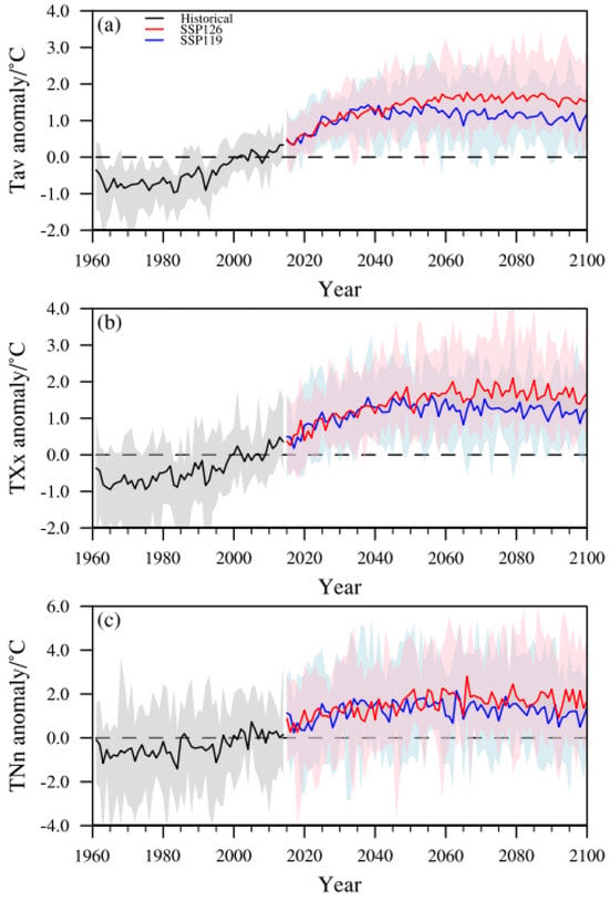
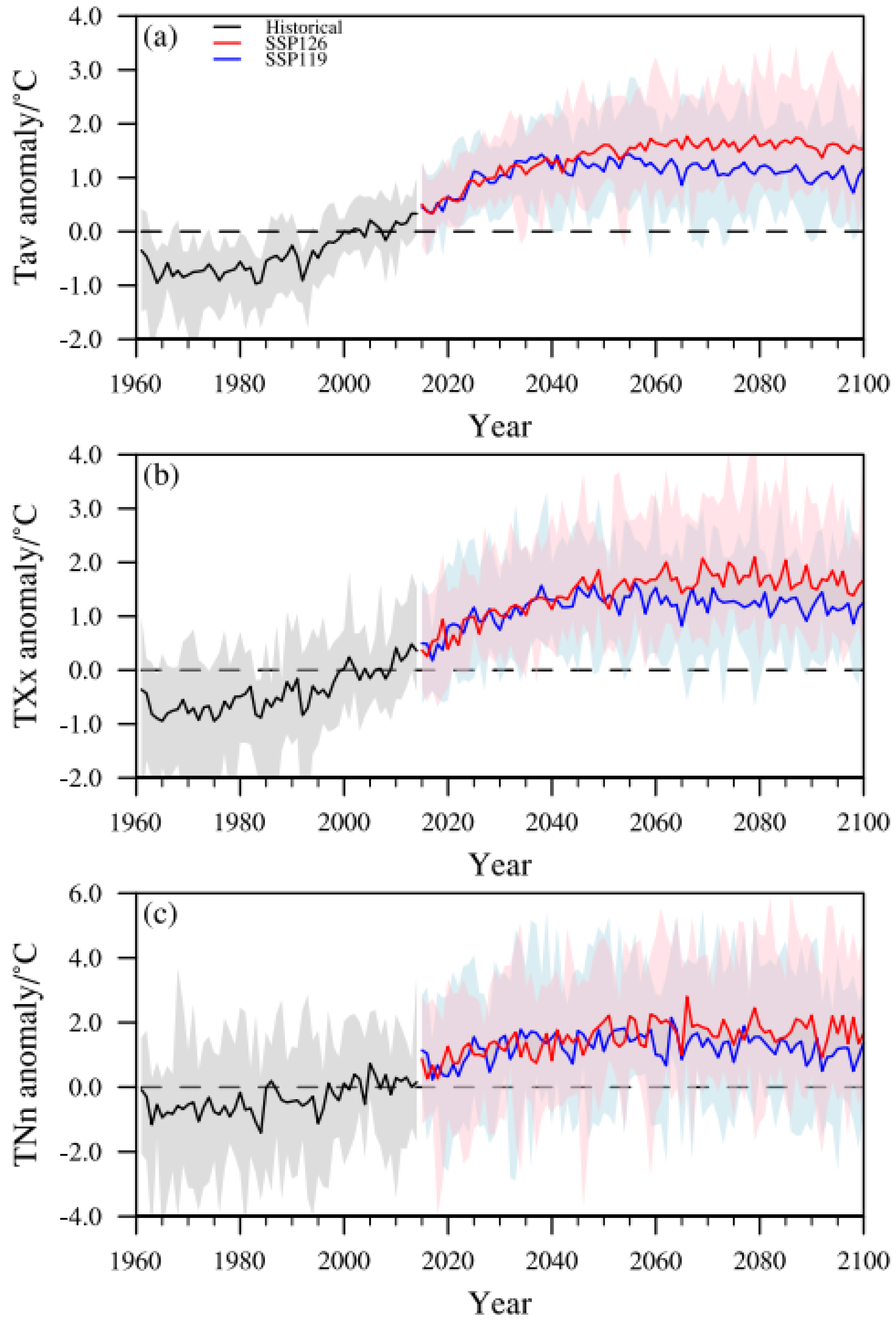
Figure 6 shows the areal-mean changes in temperature indices in China relative to the reference period (1995–2014). Temperature indices are projected to increase continuously, with stronger increases under SSP1-2.6 than under SSP1-1.9. After the carbon neutrality period, the rate of increase slows down or even slightly decreases, especially under SSP1-1.9.
Figure 6.
The time series of Tav (a), TXx (b), and TNn (c) changes compared to the baseline period (1995–2014). Solid lines denote REA, and shaded areas denote the model spread.
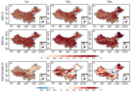
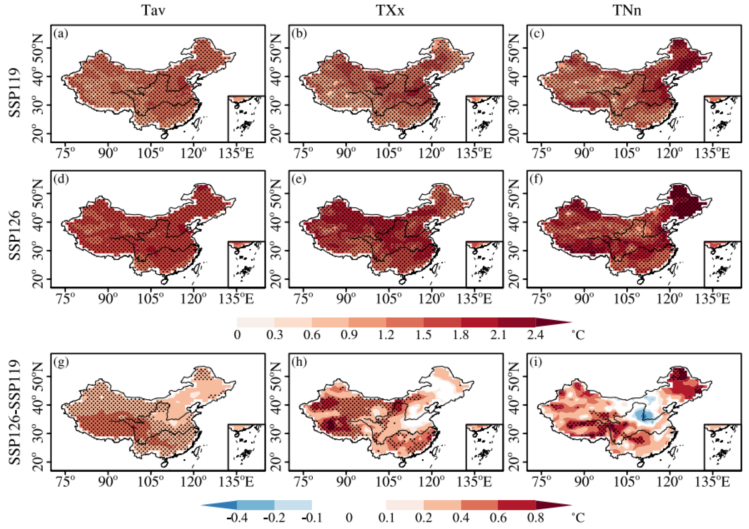
To further analyze temperature changes over China during the carbon neutrality period, Figure 7 and Figure S1 show the spatial distributions of all temperature index changes during the carbon neutrality period from REA and MME under SSP1-1.9 and SSP1-2.6, as well as their differences. The distributions of projected temperature changes are similar between the two schemes. Based on the REA, mean, and extreme temperatures are projected to increase significantly in all regions of China under both scenarios, with larger increases under the SSP1-2.6 scenario (Figure 7). The areal-mean warming over China is 1.27 °C (0.56–1.99 °C) under SSP1-1.9 and 1.61 °C (0.73–2.52 °C) under SSP1-2.6 (Table S3). The largest warming occurs in northeastern (NE) and northern (NC) China, with increases of 1.38 °C (0.37–1.94 °C) and 1.41 °C (0.72–2.27 °C) under SSP1-1.9, and 1.66 °C (0.33–2.82 °C) and 1.66 °C (0.64–2.58 °C) under SSP1-2.6. The smallest warming is found in southwestern (SW) China. These findings are consistent with previous studies [11].
Figure 7.
Projected changes, relative to 1995–2014, in Tav, TXx, and TNn under carbon neutrality in SSP1-1.9 (a–c) and SSP1-2.6 (d–f) and their differences ((g–i), SSP1-2.6 minus SSP1-1.9). Dotted regions represent significant changes at the 95% confidence level based on Student’s t test.
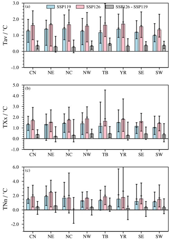
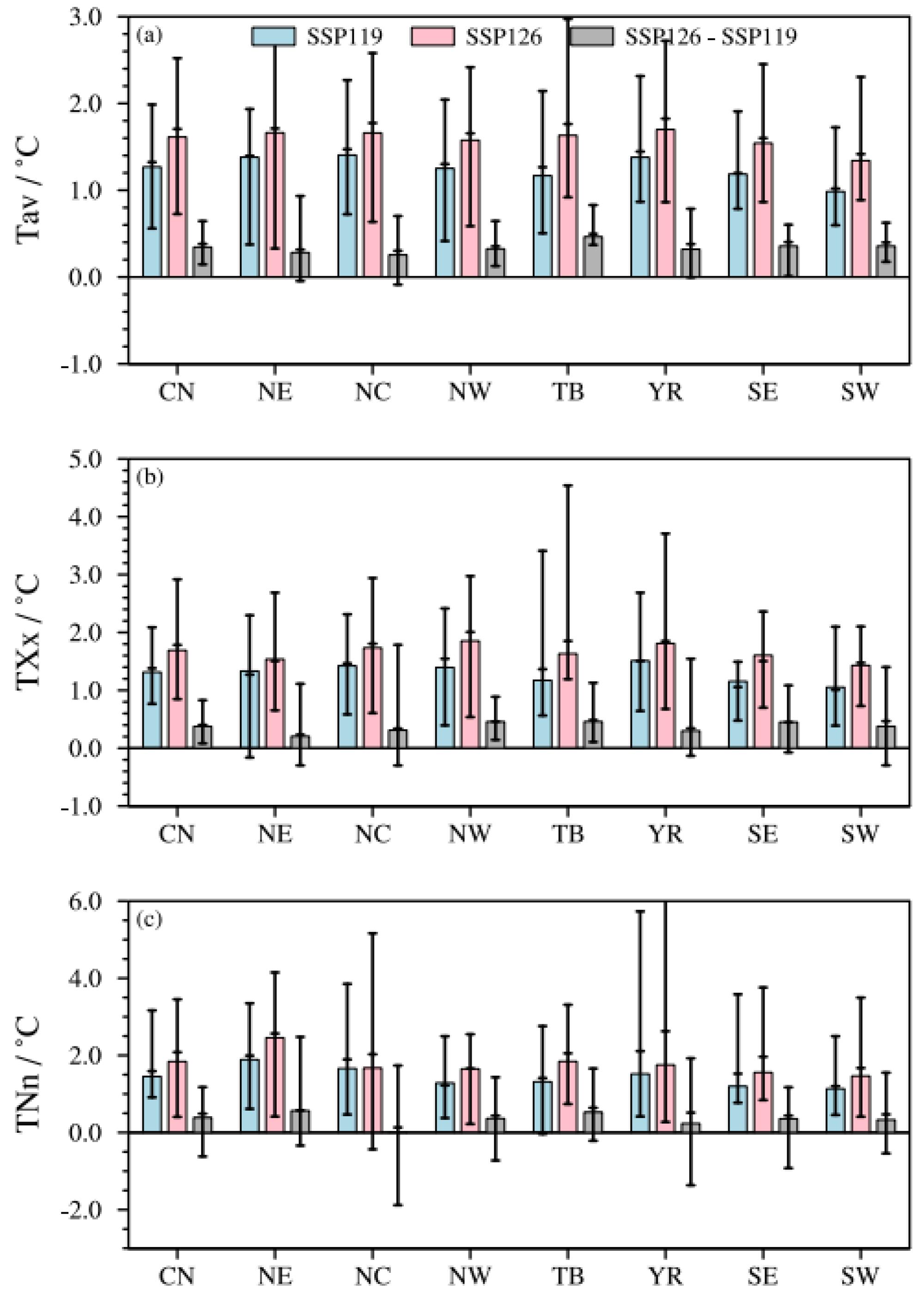
TXx and TNn also increase significantly in almost all regions under both scenarios, showing larger increases in the north and smaller increases in the south. The areal-mean increases in TXx over China are 1.31 °C (0.77–2.09 °C) and 1.69 °C (0.85–2.92 °C) under SSP1-1.9 and SSP1-2.6, respectively, while the increases in TNn are larger than those in TXx, reaching 1.45 °C (0.91–3.17 °C) and 1.84 °C (0.41–3.45 °C), respectively. The largest increases in TXx occur in NW and the mid-lower Yangtze River regions (YR), with areal-mean increases of 1.40 °C (0.39–2.42 °C) and 1.51 °C (0.64–2.69 °C) under SSP1-1.9, and 1.85 °C (0.54–2.97 °C) and 1.81 °C (0.68–3.71 °C) under SSP1-2.6 (Figure 8b and Table S3). The largest increases in TNn occur in NE, with areal-mean increases of 1.89 °C (0.61–3.35 °C) and 2.46 °C (0.42–4.15 °C) under SSP1-1.9 and SSP1-2.6, respectively, followed by NC and TB (Figure 8c and Table S3). Similar to Tav, the smallest increases in both TXx and TNn are found in SW, followed by southeastern (SE) China.
Figure 8.
The areal-mean projected changes (relative to 1995–2014) in Tav (a), TXx (b), and TNn (c) over China and the seven subregions under carbon neutrality in SSP1-1.9, SSP1-2.6, and their differences (SSP1-2.6 minus SSP1-1.9). Bars denote the REA, and horizontal lines denote the MME and inter-model range (minimum and maximum), respectively.
Comparing SSP1-1.9 (early) and SSP1-2.6 (late), the increases in mean temperature in the late period are significantly larger than those in the early period for most regions, except for parts of the NE and NC (Figure 7g). This indicates that earlier achievement of carbon neutrality targets could mitigate warming over most regions of China. Specifically, the areal-mean increases for Tav, TXx, and TNn in China during the late period are 0.34 °C (0.15–0.64 °C), 0.38 °C (0.08–0.83 °C), and 0.39 °C (−0.62–1.18 °C) higher than those during the early period, respectively (Table S3). The additional increases for Tav, TXx, and TNn in TB during the late period are 0.46 °C (0.37–0.83 °C), 0.46 °C (0.11–1.13 °C), and 0.53 °C (−0.21–1.66 °C), respectively. The difference for TNn between the early and late carbon neutrality periods is small, even negative in parts of NC. Considerable inter-model uncertainties exist there, with areal-mean increases ranging from −1.88 °C to 1.74 °C among models (Table S3).
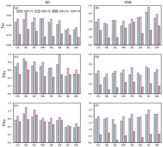
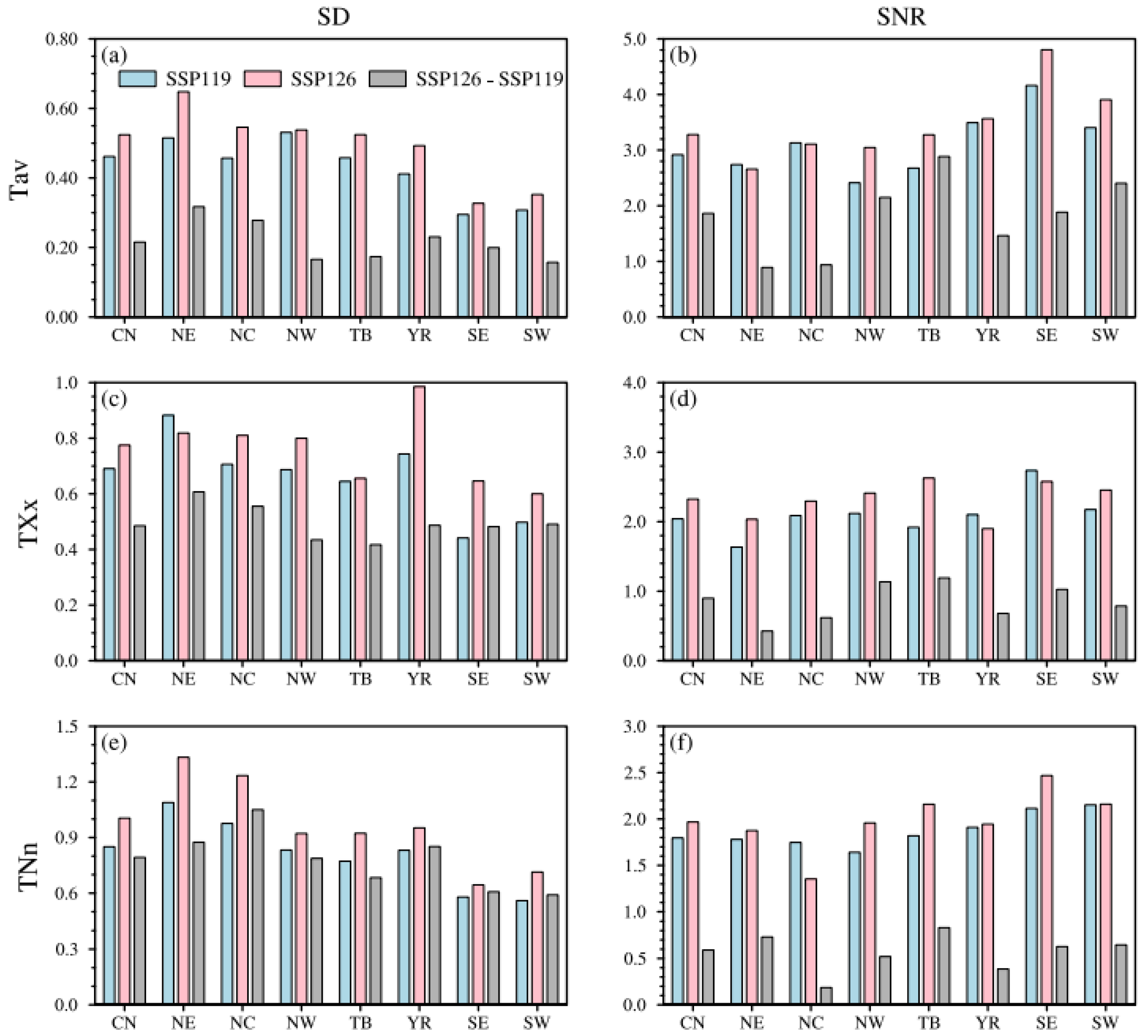
To quantitatively evaluate the uncertainty (inter-model spread) and robustness of the temperature index changes in different regions, Figure 9 shows the areal-mean inter-model standard deviation (SD) and signal-to-noise ratio (SNR) of China and its seven subregions based on REA under two scenarios. Results show that the SNR (SD) is generally larger (smaller) than 1.6 (1) for all temperature indices under both scenarios, except for TNn in NE and NC (Table S5), which indicates robust temperature projections in China. The projections for Tav are more robust than those for TXx and TNn, with smaller SDs and larger SNRs. Comparing different regions, areas with stronger warming tend to have larger SDs and smaller SNRs. Among the seven sub-regions, northeastern China has the largest model spread, with SDs for TNn reaching 1.09 and 1.33 under SSP1-1.9 and SSP1-2.6, respectively. The SNR is contrary to the SD. The largest SNR for Tav is in SE (above 4.1 in both periods), while the smallest is in NE (below 2.8 under both scenarios). Although the warming signal is large in NE, the noise (spread among models) is much larger, which leads to smaller SNR over there. It is clear that temperature projections are most robust in SE and least robust in NE. Comparing the differences between early and late carbon neutrality periods, SDs are smaller than those in the two individual periods, and SNRs are also smaller. SNRs are even less than 1 for TNn among all regions.
Figure 9.
The areal-mean standard deviation (SD, (a,c,e)) and signal-to-noise ratio (SNR, (b,d,f)) of Tav (a,b), TXX (c,d), and TNn (e,f) over China and its seven subregions by REA under carbon neutrality in SSP1-1.9, SSP1-2.6, and their differences (SSP1-2.6 minus SSP1-1.9).
3.3.2. Changes in Extreme Precipitation
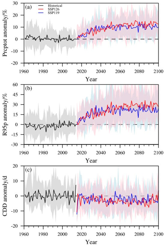
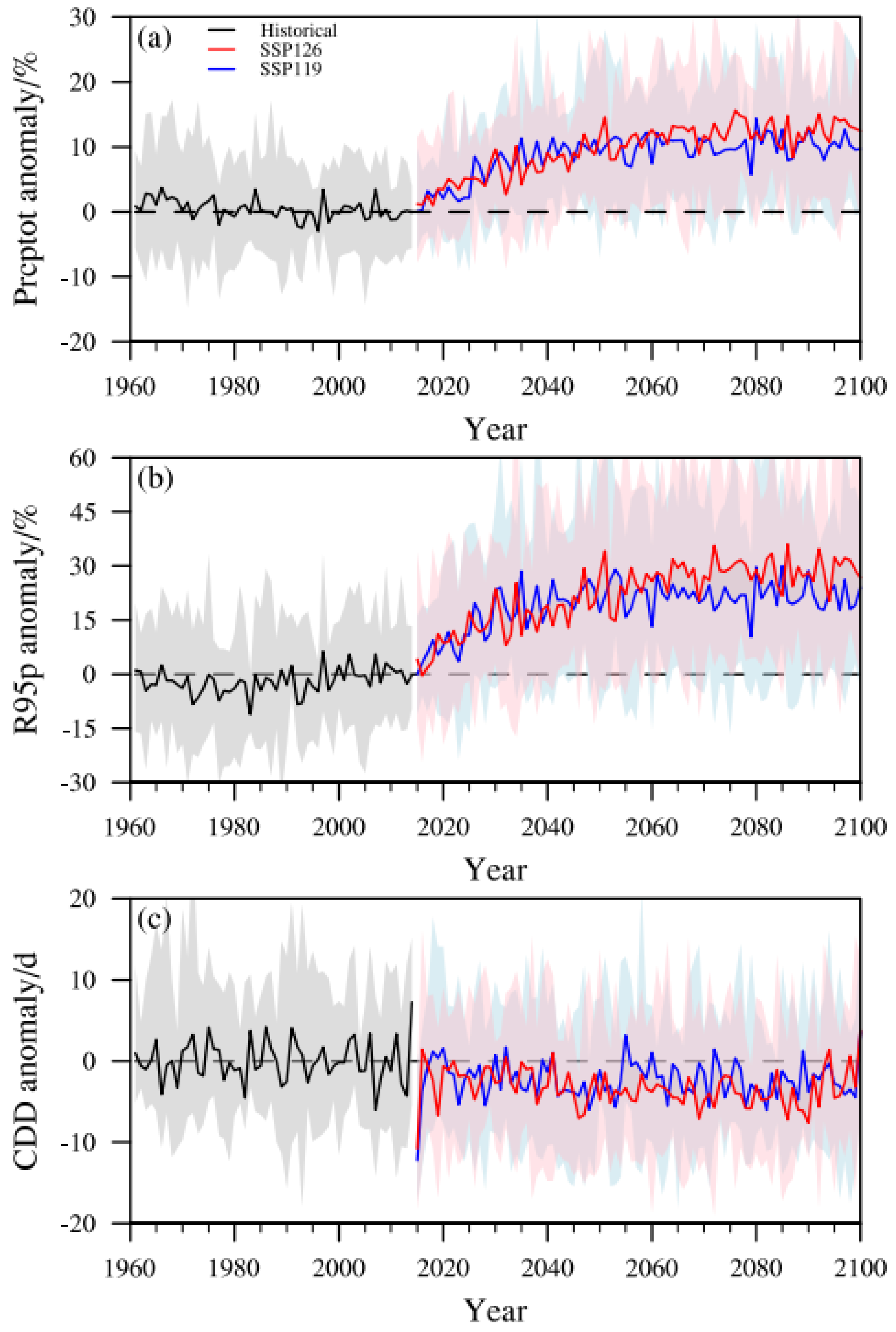
Figure 10 shows the areal-mean changes in precipitation indices in China relative to the reference period, where Prcptot and R95p are shown as relative changes, and CDD is shown as an absolute change. Prcptot and R95p are projected to increase continuously, with slightly stronger increases under SSP1-2.6 than under SSP1-1.9. After the carbon neutrality period, the rate of increase in precipitation indices recedes or slightly decreases, with a more obvious decrease under the SSP1-1.9 scenario. CDD is projected to decrease, with little difference between the two scenarios.
Figure 10.
The time series of Prcptot (a), R95p (b), and CDD (c) changes compared to the baseline period. Solid lines denote REA, and shaded areas denote the model spread.
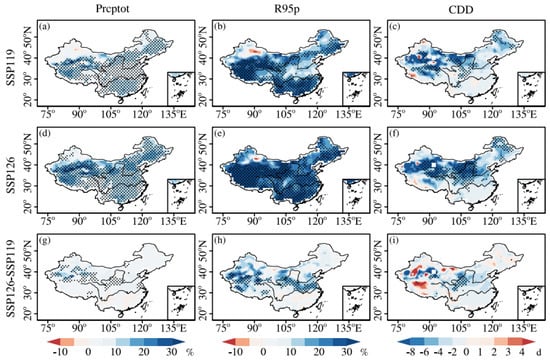
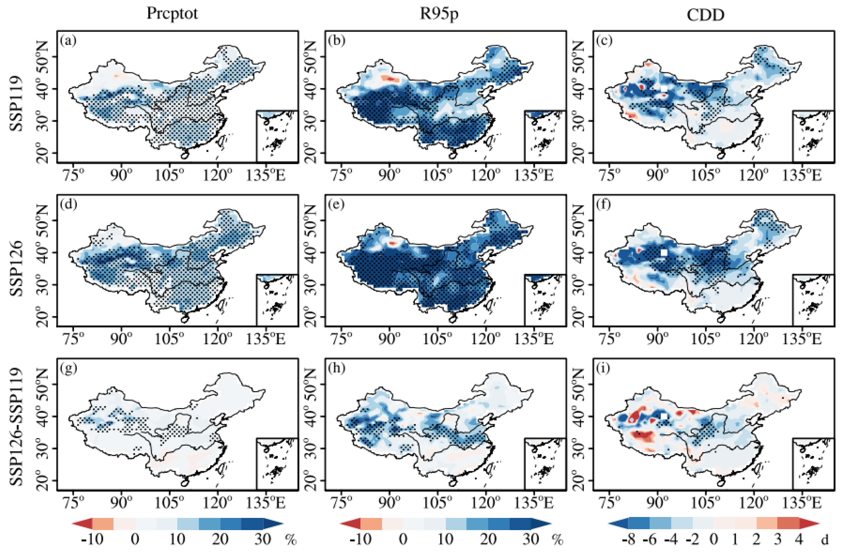
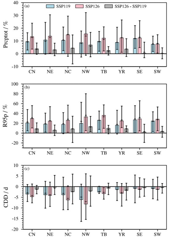
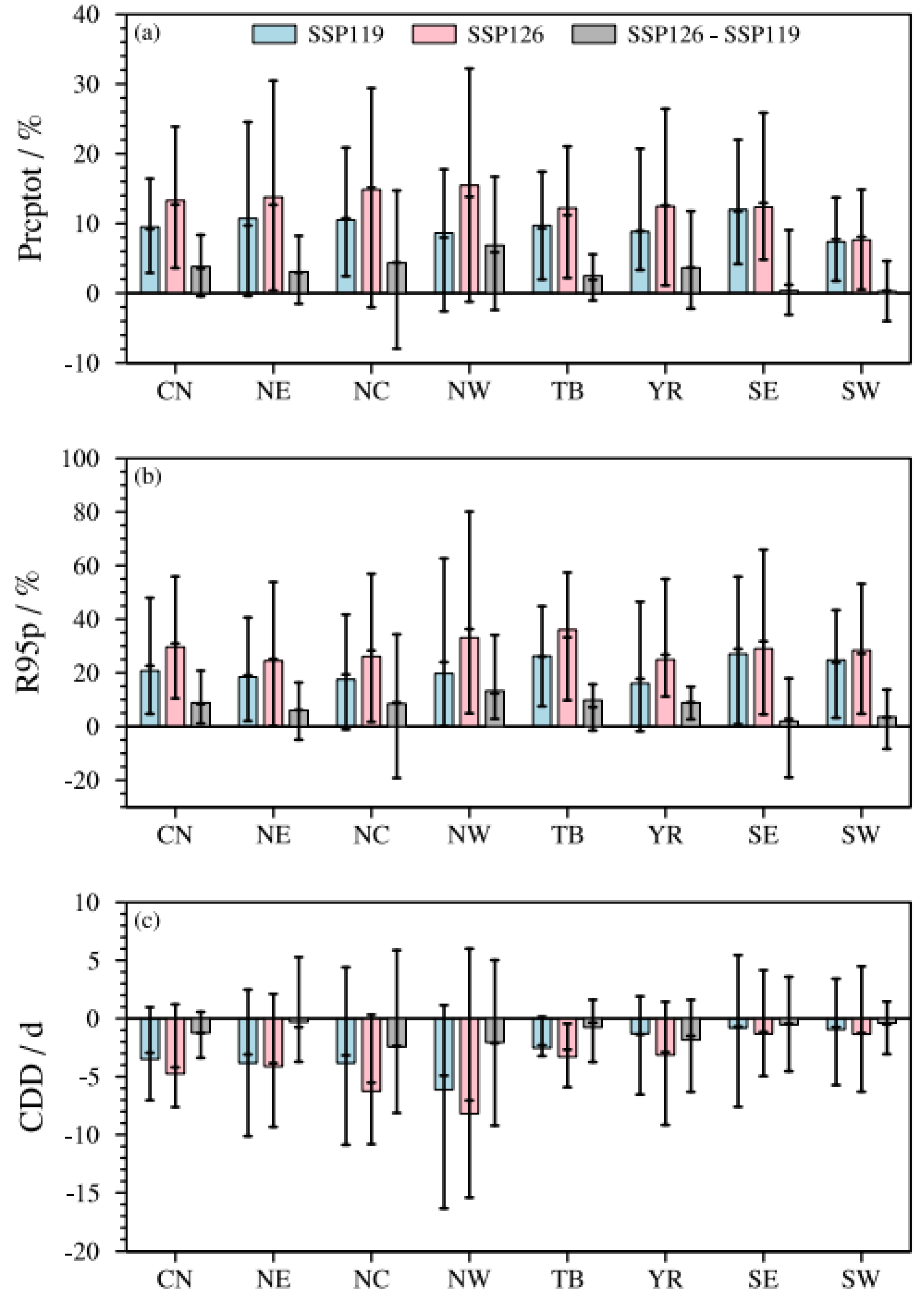
To further analyze the characteristics of extreme precipitation changes over China during the carbon neutrality period, Figure 11 and Figure S2 show the spatial distributions of all precipitation index changes from REA and MME during the carbon neutrality period under SSP1-1.9 and SSP1-2.6, as well as their differences. Like the temperature indices, the projected precipitation changes show similar distributions between the two schemes. Mean and extreme precipitation increase significantly in almost all regions of China under both scenarios, with larger increases under SSP1-2.6. However, the changes are not significant for Prcptot in parts of northern Xinjiang, for R95p in parts of northern Xinjiang, and a few areas of eastern China north of the Yangtze River (Figure 11). The areal-mean increases for Prcptot over China are 9.5% (2.9–16.4%) under SSP1-1.9 and 13.3% (3.6–23.9%) under SSP1-2.6. Relatively large increases are noted across SE (12.0%), NE (10.7%), and NC (10.5%) under SSP1-1.9. Larger increases are found in NW (15.5%), NC (14.9%), and NE (13.8%) under SSP1-2.6 (Figure 12 and Table S4). These findings are consistent with previous studies [11]. The increases for R95p are larger than those for Prcptot, with areal-mean increases of 20.8% (4.7–48.0%) and 29.6% (10.4–55.9%) under SSP1-1.9 and SSP1-2.6, respectively. Larger increases are found for R95p in SE (27.0%), TB (26.3%), and SW (24.8%) under SSP1-1.9. The largest increases occur in TB (36.1%) and NW (33.1%) under SSP1-2.6. R95p decreases in some regions of northern Xinjiang, although these changes are not significant (Figure 11b,e). It is worth noting that relative changes can be large in arid regions (like NW and TB), while the corresponding absolute changes remain small. Taking NW as an example, the absolute areal-mean increases for Prcptot (R95p) are only 14.0 mm (7.1 mm) under SSP1-1.9 and 24.2 mm (12.0 mm) under SSP1-2.6, while their relative increases are 8.6% (17.8%) and 15.5% (32.2%). CDD shows a north–south contrast, with significant decreases in parts of northern China but little change in southern China during the carbon neutrality periods.
Figure 11.
Projected changes, relative to 1995–2014, in Prcptot, R95p, and CDD under carbon neutrality in SSP1-1.9 (a−c) and SSP1-2.6 (d−f) and their differences ((g−i), SSP1-2.6 minus SSP1-1.9). Dotted regions represent significant changes at the 95% confidence level based on Student’s t test.
Figure 12.
The areal-mean projected changes (relative to 1995–2014) in Prcptot (a), R95p (b), and CDD (c) over China and the seven subregions under carbon neutrality in SSP1-1.9, SSP1-2.6, and their differences (SSP1-2.6 minus SSP1-1.9). Bars denote the REA, and horizontal lines denote the MME and inter-model range (minimum and maximum), respectively.
Comparing SSP1-1.9 (early) and SSP1-2.6 (late), the increases for Prcptot and R95p in the late period are larger than those in the early period for most regions, with the areal-mean differences of 3.8% (−0.4–8.4%) and 8.8% (1.1–20.8%) in China, respectively. This indicates that, to some extent, earlier achievement of carbon neutrality targets could reduce precipitation increases over most of China. This is especially true in NW, where the increases in Prcptot and R95p during the late period are 6.9% (−2.4–16.7%) and 13.3% (2.9–34.1%) higher than those during the early period (Figure 12 and Table S4). The difference between early and late carbon neutrality periods is small for CDD, with only a few regions in the upper reaches of the Yellow River showing larger decreases during the late period.
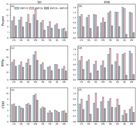
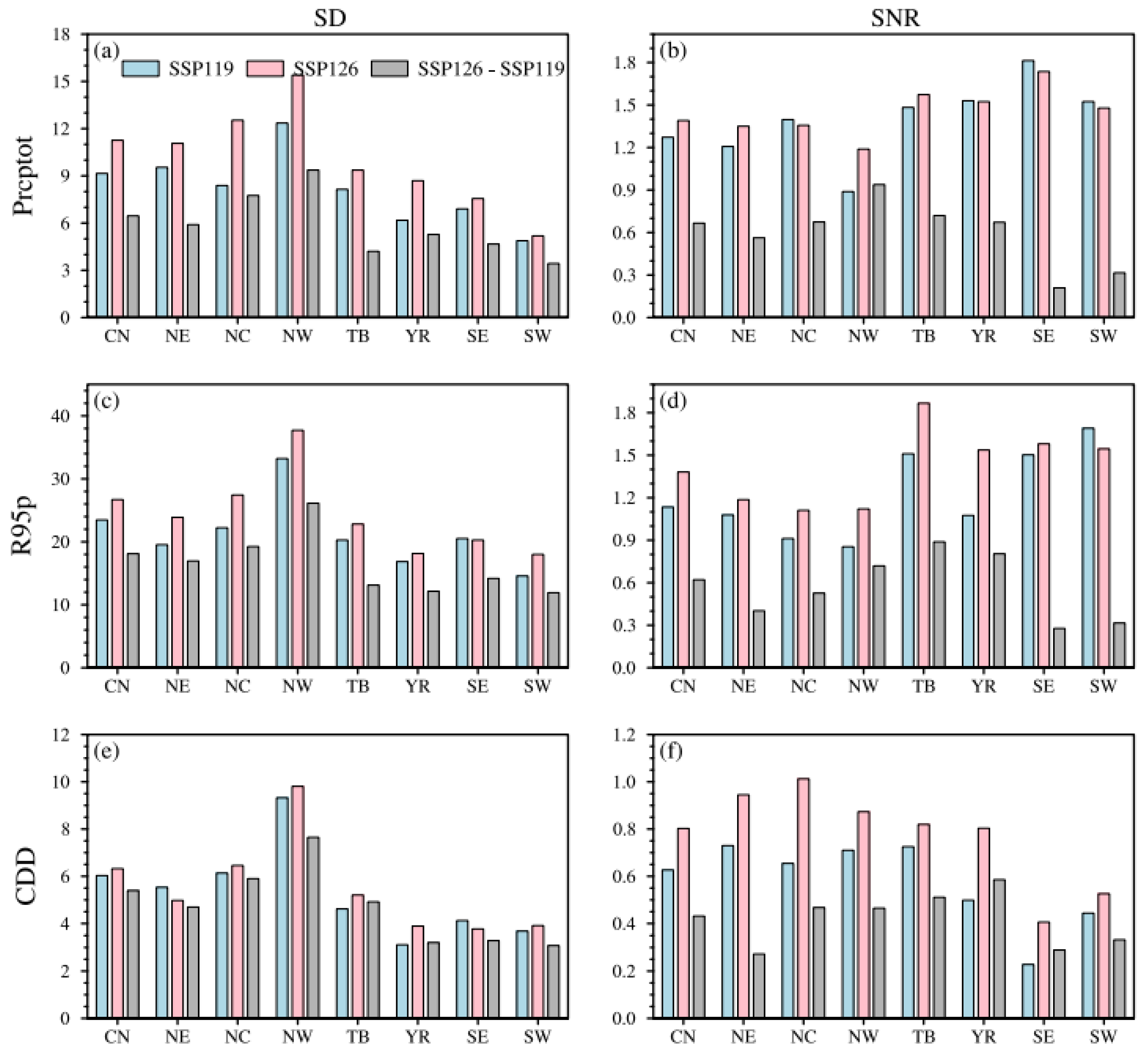
Figure 13 shows the areal-mean inter-model standard deviation (SD) and signal-to-noise ratio (SNR) for precipitation indices of China and its seven subregions based on REA under two scenarios. Precipitation indices show larger SDs and smaller SNRs than temperature indices, indicating that precipitation projections are less robust than temperature projections. The projections for Prcptot are slightly more robust than those for R95p, with smaller SDs and larger SNRs. The projections for CDD are the least robust, with SNRs less than 1 (Table S5). Projection uncertainty is larger in northern China than in southern China. The largest uncertainty occurs in NW, with SDs for R95p exceeding 33.2% and 37.7% under SSP1-1.9 and SSP1-2.6. SW has the smallest SDs, which are 14.6% and 18.0% under SSP1-1.9 and SSP1-2.6. The SNR is contrary to the SD. The smallest SNR for Prcptot and R95p is in NW (less than 1) under SSP1-1.9. The relatively large SNRs are in SW and SE, with areal-mean values greater than 1.5 under both scenarios, indicating robust precipitation projections in these regions. Although the change signal in these regions is not large, the noise is much smaller, resulting in a large SNR. Comparing the differences between early (SSP1-1.9) and late (SSP1-2.6) carbon neutrality periods, SDs are smaller than those in the two individual periods, and SNRs are also smaller, with areal-mean SNRs less than 1 for all precipitation indices in all regions. In summary, precipitation projections are most robust in SW and least robust in NW.
Figure 13.
The areal-mean standard deviation (SD, (a,c,e)) and signal-to-noise ratio (SNR, (b,d,f)) of Prcptot (a,b), R95p (c,d), and CDD (e,f) over China and its seven subregions by REA under carbon neutrality in SSP1-1.9, SSP1-2.6, and their differences (SSP1-2.6 minus SSP1-1.9).
4. Discussion
This study systematically quantifies the differential impacts of the timing of carbon neutrality (early versus late) on mean and extreme climates over China under low-emission (SSP1-1.9 and SSP1-2.6) scenarios. The results show that earlier achievement of carbon neutrality targets could help mitigate future warming and precipitation increases in China, and to some extent reduce the intensification of extreme warm events over the Tibetan Plateau and extreme wet events in northwestern China. These findings can provide a scientific basis for climate adaptation and mitigation policies.
Unlike previous studies focusing on mean temperature and precipitation changes during the carbon neutrality period [11], this study pays more attention to the impacts of carbon neutrality target achievement on extreme climate changes in multiple climate change hotspots in China. For example, the Tibetan Plateau is highly sensitive to climate change. Extreme events over this region have increased under global warming [36,37], threatening the cryosphere and ecosystems [38,39]. However, early achievement of carbon neutrality targets could help reduce future increases in extreme high temperatures and extreme precipitation events over there, which are important for ecological protection and sustainable development in this region. Northwestern China is an arid inland region, where future increases in extreme temperatures will increase the risks of land degradation and desertification [40,41], and extreme precipitation events are also projected to increase significantly under warmer conditions [42]. Early achievement of the carbon neutrality target may, to some degree, help reduce these risks.
This study focuses on regional climate responses in China under low-emission (SSP1-1.9 and SSP1-2.6 her) scenarios that can achieve carbon neutrality targets. Many studies have focused on high-emission scenarios (such as SSP5-8.5) [6,11,14,23,32], and we do not directly compare their differences here. The achievement of carbon neutrality targets has positive impacts on regional mean and extreme climate changes in China, reducing the intensification of extreme warm events and wet events in northwestern China and the Tibetan Plateau [14]. However, studies on risks and impacts of climate responses under carbon neutrality targets, such as population exposure, have not yet been conducted. The potential causes and physical mechanisms underlying these future changes also need to be further explored.
Previous studies suggest that the strong warming over the Tibetan Plateau may be associated with changes in shortwave radiation [40] and snow/ice albedo feedback [37]. The increase in atmospheric moisture under warming [43], and the enhanced transport of water vapor caused by the strengthening of the westerly wind circulation [44] could contribute to the large increase in precipitation in northwestern China. The subregions in eastern China are strongly influenced by the East Asian monsoon [45]. Changes in the monsoon circulation could affect the precipitation over these regions [46]. The precipitation in southwestern China is largely influenced by the South Asian summer monsoon [47] and the moisture transport from the Indian Ocean [48]. Overall, the increase in precipitation under warming is primarily attributed to the increase in moisture convergence, which comes mainly from the thermodynamic effect due to increasing atmospheric moisture [43,46]. The dynamic effect, such as monsoon circulation changes, dominates regional differences in the projected precipitation changes [46]. In terms of the contrasting responses of CDD and precipitation, many factors other than global warming may also play a role at the regional scale, including local feedbacks [49] and local-scale external forcings, such as aerosol concentrations [50], land use and land cover changes [51]. A better understanding of complex drivers controlling regional climate changes, including climate system internal feedbacks and external forcings, is an urgent issue for future studies.
It should also be noted that uncertainties exist in the results of this study on regional climate responses under carbon neutrality targets in China. On the one hand, the timing of global carbon neutrality in this study is determined solely by CO2 concentration, which introduces uncertainty. On the other hand, model simulation performance varies due to different physical frameworks, parameterization settings, and resolutions [17,19]. Only 12 models are currently available for the SSP1-1.9 scenario, which is a relatively small number and may affect the robustness of the projections. More models need to be added in future work. Our analysis is based on one single realization (member) per model, which means that the reported spread primarily represents inter-model uncertainty and does not account for internal variability. Internal variability typically plays an important role in the nearer term, at local spatial scales, and in spatially and temporally heterogeneous variables such as precipitation [52]. It can be isolated from model uncertainty using large ensembles [53].
Only two SSP1 pathways (SSP1-2.6 and SSP1-1.9) are considered. Although these capture the low-emission range most relevant to carbon neutrality [18], they do not span the full range of plausible futures, and our findings may therefore not generalize to higher-emission scenarios. In addition, the contrast between these two pathways is used in this work to assess the climate response to early versus late carbon neutrality. This contrast thus reflects both temporal and emission scenario differences, a point that should be kept in mind when interpreting the results.
Observational uncertainty is non-negligible, especially for precipitation in regions with sparse gauge coverage (e.g., the Tibetan Plateau and parts of the continental interior). These can affect both the evaluation of present-day model performance and the derived observational constraints. Although the REA method adopted here reduces uncertainty to some extent, it assigns model weights based on present-day performance. REA still overestimates precipitation (Prcptot and R95p) over China, which may reduce confidence in the magnitude of the projected precipitation changes, even though the sign of the projections can still be robust. Other advanced multi-model ensemble methods based on different constraint ideas have emerged in recent years [54], including performance-based weighting [7,55], emergent constraints [56,57], attribution constraints [58,59], and artificial intelligence approaches [60,61]. These methods hold considerable promise for climate projections under carbon neutrality targets.
5. Conclusions
This study used CMIP6 model simulations, including historical experiments and future scenario (SSP1-1.9 and SSP1-2.6) projections. The models’ ability to simulate climate extreme indices over China was first evaluated, and the performance of our improved reliability ensemble averaging (REA) method was compared with that of the unweighted multi-model ensemble mean (MME). The REA method was then used to project changes in climate extremes over China under carbon neutrality in SSP1-1.9 and SSP1-2.6, as well as the differences between them. The spatial characteristics, uncertainties, and robustness of future projections across different regions are also analyzed. The main findings are summarized as follows:
CMIP6 models demonstrate better performance in simulating the spatial pattern of temperature and precipitation indices over China, with noteworthy performance for temperature indices compared to that of precipitation indices. The REA method outperforms the MME in simulating all climate indices in China.
The timing of global carbon neutrality under the two scenarios was determined based on the peak time of CO2 mass, with carbon neutrality reached in 2042 under SSP1-1.9 and in 2063 under SSP1-2.6.
Relative to the historical period (1995–2014), mean and extreme temperatures increase significantly across China under both scenarios, with larger increases under SSP1-2.6. The areal-mean increases in China for Tav, TXx, and TNn under SSP1-1.9 are 1.27 °C (0.56–1.99 °C), 1.31 °C (0.77–2.09 °C), and 1.45 °C (0.91–3.17 °C), respectively. Those under SSP1-2.6 are 1.61 °C (0.73–2.52 °C), 1.69 °C (0.85–2.92 °C), and 1.84 °C (0.41–3.45 °C), respectively. Larger increases for Tav and TNn are noted in NE and NC, while larger increases for TXx are detected in NW and YR. Temperature projections are most robust in SE, with the largest SNR, and least robust in NE, with the smallest SNR.
Like temperature indices, mean and extreme precipitation also increase significantly across China under both scenarios, with larger increases under SSP1-2.6. CDD decreases in northern China but shows little change in southern China. The areal-mean increases in China for Prcptot under SSP1-1.9 and SSP1-2.6 are 9.5% (2.9–16.4%) and 13.3% (3.6–23.9%), while for R95p they are 20.8% (4.7–48.0%) and 29.6% (10.4–55.9%), respectively. The largest increases for Prcptot occur in TB and NE, while for R95p they occur in TB and the regions south of the Yangtze River. The smallest but most robust precipitation increases are in SW, while the least robust is in NW.
The times to achieve carbon neutrality target differ between the two scenarios. Compared with late carbon neutrality under SSP1-2.6, early carbon neutrality under SSP1-1.9 can reduce warming and precipitation increases in China. The areal-mean increases for Tav, TXx, TNn, Prcptot, and R95p during the early carbon neutrality period are 0.34 °C, 0.38 °C, 0.39 °C, 3.8%, and 8.8% lower than those during the late carbon neutrality period. Earlier achievement of carbon neutrality can greatly suppress warming in TB, and to some extent reduce the increases in mean and extreme precipitation in NW.
Supplementary Materials
The following supporting information can be downloaded at: https://www.mdpi.com/article/10.3390/atmos17111080/s1, Figure S1: Projected changes, relative to 1995–2014, in Tav, TXx, and TNn under carbon neutrality in SSP1-1.9 (a–c) and SSP1-2.6 (d–f) and their differences (g–i, SSP1-2.6 minus SSP1-1.9) from MME; Figure S2: Projected changes, relative to 1995–2014, in Prcptot, R95p, and CDD under carbon neutrality in SSP1-1.9 (a–c) and SSP1-2.6 (d–f) and their differences (g–i, SSP1-2.6 minus SSP1-1.9) from MME; Table S1: PCC, RSD, CRMSE, and IVS of 12 CMIP6 models, MME, and REA.; Table S2: The areal-mean biases (simulation minus observation) of all indices in MME and REA for 1995–2014; Table S3: The areal-mean changes in temperature indices over China and the seven subregions; Table S4: The areal-mean changes in precipitation indices over China and the seven subregions; Table S5: The areal-mean SD and SNR of all indices in REA over China and the seven subregions.
Author Contributions
Conceptualization, H.Z.; methodology, H.Z.; software, H.Z.; validation, H.Z. and B.O.A.; formal analysis, H.Z.; investigation, H.Z.; resources, H.Z.; data curation, H.Z. and B.O.A.; writing—original draft preparation, H.Z. and B.O.A.; writing—review and editing, H.Z. and B.O.A.; visualization, H.Z.; supervision, H.Z. and B.O.A.; project administration, H.Z.; funding acquisition, H.Z. All authors have read and agreed to the published version of the manuscript.
Funding
This research was funded by the National Natural Science Foundation of China (42505169), the Basic Research Program of Jiangsu (BK20240317), the Wuxi University Research Start-up Fund for Introduced Talents (2024r041).
Institutional Review Board Statement
Not applicable.
Informed Consent Statement
Not applicable.
Data Availability Statement
All the datasets used in this study are from open-source platforms available via https://esgf-node.llnl.gov/projects/esgf-llnl (accessed on 1 September 2026) for the CMIP6 models.
Acknowledgments
The authors appreciate the data sources for freely providing the data used in this study.
Conflicts of Interest
The authors declare no conflicts of interest.
Abbreviations
The following abbreviations are used in this manuscript:
| AR6 | Sixth Assessment Report |
| CDD | Consecutive dry days |
| CMIP6 | Coupled Model Intercomparison Project Phase 6 |
| CN | China |
| CRMSE | Centered root mean square error |
| GCM | Global Climate Model |
| GMST | Global mean surface temperature |
| IPCC | Intergovernmental Panel on Climate Change |
| IVS | Interannual variability skill score |
| MME | Multi-model ensemble mean |
| NC | Northern China |
| NE | Northeastern China |
| NW | Northwestern China |
| PCC | Pattern correlation coefficient |
| Prcptot | Total precipitation |
| R95p | Heavy precipitation |
| REA | Reliability ensemble averaging |
| RSD | Ratio of spatial standard deviation |
| SD | Standard deviation |
| SE | Southeastern China |
| SNR | Signal-to-noise ratio |
| SSP | Shared Socioeconomic Pathways |
| STD | Temporal standard deviation |
| SW | Southwestern China |
| Tav | Mean temperature |
| TB | Tibetan Plateau |
| TNn | Coldest night temperature |
| TXx | Hottest day temperature |
| YR | The mid-lower Yangtze River regions |
Appendix A
Table A1.
Model numbers, model names, modeling centers and countries, IDs, as well as the atmospheric resolutions, of 12 CMIP6 global climate models.
Table A2.
CO2 data used in this article. Years in the table show when each model reaches carbon neutrality.
References
- IPCC. Summary for Policymakers. In Climate Change 2021: The Physical Science Basis. Contribution of Working Group I to the Sixth Assessment Report of the Intergovernmental Panel on Climate Change; Cambridge University Press: Cambridge, UK; New York, NY, USA, 2021; pp. 3–32. [Google Scholar]
- Allen, M.; Frame, D.; Huntingford, C.; Jones, C.; Lowe, J.; Meinshausen, M.; Meinshausen, N. Warming caused by cumulative carbon emissions towards the trillionth tonne. Nature 2009, 458, 1163–1166. [Google Scholar] [CrossRef] [Scilit] [PubMed]
- Stocker, B.; Roth, R.; Joos, F.; Spahni, R.; Steinacher, M.; Zaehle, S.; Bouwman, L.; Ri, X.; Prentice, I. Multiple greenhouse-gas feedbacks from the land biosphere under future climate change scenarios. Nat. Clim. Change 2013, 3, 666–672. [Google Scholar] [CrossRef] [Scilit]
- Chen, H.; Sun, J.; Lin, W.; Xu, H. Comparison of CMIP6 and CMIP5 models in simulating climate extremes. Sci. Bull. 2020, 65, 1415–1418. [Google Scholar] [CrossRef] [Scilit] [PubMed]
- Kim, Y.; Min, S.; Zhang, X.; Sillmann, J.; Sandstad, M. Evaluation of the CMIP6 multi-model ensemble for climate extreme indices. Weather Clim. Extrem. 2020, 29, 100269. [Google Scholar] [CrossRef] [Scilit]
- Zhu, H.; Jiang, Z.; Li, L. Projection of climate extremes in China, an incremental exercise from CMIP5 to CMIP6. Sci. Bull. 2021, 66, 2528–2537. [Google Scholar] [CrossRef] [Scilit] [PubMed]
- Zhu, H.; Jiang, Z.; Li, L.; Li, W.; Jiang, S.; Zhou, P.; Zhao, W.; Li, T. Intercomparison of multi-model ensemble-processing strategies within a consistent framework for climate projection in China. Sci. China Earth Sci. 2023, 66, 2125–2141. [Google Scholar] [CrossRef] [Scilit]
- UNFCCC. Adoption of the Paris Agreement; United Nations Office at Geneva SU: Geneva, Switzerland, 2015. [Google Scholar]
- You, Q.; Jiang, Z.; Yue, X.; Guo, W.; Liu, Y.; Cao, J.; Li, W.; Wu, F.; Cai, Z.; Zhu, H.; et al. Recent frontiers of climate changes in East Asia at global warming of 1.5 °C and 2.0 °C. npj Clim. Atmos. Sci. 2022, 5, 80. [Google Scholar] [CrossRef] [Scilit]
- Chen, J.; Cui, H.; Xu, Y.; Ge, Q. Long-term temperature and sea-level rise stabilization before and beyond 2100: Estimating the additional climate mitigation contribution from China’s recent 2060 carbon neutrality pledge. Environ. Res. Lett. 2021, 16, 074032. [Google Scholar] [CrossRef] [Scilit]
- Deng, L.; Zhu, H.; Jiang, Z. Projection of climate change in China under carbon neutral scenarios. Trans. Atmos. Sci. 2022, 45, 364–375. (In Chinese) [Google Scholar]
- Zhang, J.; You, Q. Avoidable heat risk under scenarios of carbon neutrality by mid-century. Sci. Total Environ. 2023, 892, 164679. [Google Scholar] [CrossRef] [Scilit] [PubMed]
- Xiang, X.; Wang, W.; Wu, X.; Zhu, L.; Adnan, R.; Wu, L.; Cao, H.; Lin, X.; Liu, Y. Effects of deep learning bias correction and carbon neutrality on projections of future population exposure to extreme precipitation. Int. J. Climatol. 2026, 46, e70174. [Google Scholar] [CrossRef] [Scilit]
- Cai, Z.; You, Q.; Wu, F.; Jiang, Z.; Zhai, P. China’s climate and extreme climate changes under the global carbon neutrality scenario. Sci. Technol. Rev. 2024, 42, 73–84. (In Chinese) [Google Scholar]
- Yang, C.; Wang, Y.; Su, B.; Pu, Y.; Wang, Y.; Jiang, T. Runoff variation trend of Ganjiang River Basin under SSP “Double Carbon” path. Clim. Change Res. 2022, 18, 177–187. (In Chinese) [Google Scholar]
- Wang, J.; Liang, P.; Cheng, F.; Liu, Y.; Song, C.; Wu, W.; Zheng, Q.; Zhang, T.; Qu, P.; Li, Y.; et al. Evaluation and projection of circulation conditions tied to summertime compound drought and heatwave frequency over the Yangtze River Delta, China, for the carbon neutrality period based on CMIP6 GCMs. Int. J. Climatol. 2024, 44, 2739–2757. [Google Scholar] [CrossRef] [Scilit]
- Eyring, V.; Bony, S.; Meehl, G.; Senior, C.; Stevens, B.; Stouffer, R.; Taylor, K. Overview of the Coupled Model Intercomparison Project Phase 6 (CMIP6) experimental design and organization. Geosci. Model Dev. 2016, 9, 1937–1958. [Google Scholar] [CrossRef] [Scilit]
- O’Neill, B.; Tebaldi, C.; van Vuuren, D.; Eyring, V.; Friedlingstein, P.; Hurtt, G.; Knutti, R.; Kriegler, E.; Lamarque, J.; Lowe, J.; et al. The scenario model intercomparison project (ScenarioMIP) for CMIP6. Geosci. Model Dev. 2016, 9, 3461–3482. [Google Scholar] [CrossRef] [Scilit]
- Zhou, T.; Zou, L.; Chen, X. Commentary on the coupled model intercomparison project phase 6 (CMIP6). Clim. Change Res. 2019, 15, 445–456. (In Chinese) [Google Scholar]
- Xu, Y.; Han, Z.; Wu, J.; Li, R. The differences of global extreme climate events changes before and after 1.5 °C overshoot. Clim. Change Res. 2024, 20, 389–402. (In Chinese) [Google Scholar]
- Zhu, H.; Jiang, Z.; Li, J.; Li, W.; Sun, C.; Li, L. Does CMIP6 inspire more confidence in simulating climate extremes over China? Adv. Atmos. Sci. 2020, 37, 1119–1132. [Google Scholar] [CrossRef] [Scilit]
- Jiang, D.; Hu, D.; Tian, Z.; Lang, X. Differences between CMIP6 and CMIP5 models in simulating climate over China and the East Asian monsoon. Adv. Atmos. Sci. 2020, 37, 1102–1118. [Google Scholar] [CrossRef] [Scilit]
- Yang, X.; Zhou, B.; Xu, Y.; Han, Z. CMIP6 evaluation and projection of temperature and precipitation over China. Adv. Atmos. Sci. 2021, 38, 817–830. [Google Scholar] [CrossRef] [Scilit]
- Xin, X.; Wu, T.; Zhang, J.; Yao, J.; Fang, Y. Comparison of CMIP6 and CMIP5 simulations of precipitation in China and the East Asian summer monsoon. Int. J. Climatol. 2020, 40, 6423–6440. [Google Scholar] [CrossRef] [Scilit]
- Chen, W.; Jiang, Z.; Li, L. Probabilistic projections of climate change over China under the SRES A1B scenario using 28 AOGCMs. J. Clim. 2011, 24, 4741–4756. [Google Scholar] [CrossRef] [Scilit]
- Li, W.; Jiang, Z.; Xu, J.; Li, L. Extreme precipitation indices over China in CMIP5 models. Part II: Probabilistic projection. J. Clim. 2016, 29, 8989–9004. [Google Scholar] [CrossRef] [Scilit]
- Knutti, R.; Sedláček, J.; Sanderson, B.; Lorenz, R.; Fischer, E.; Eyring, V. A climate model projection weighting scheme accounting for performance and interdependence. Geophys. Res. Lett. 2017, 44, 1909–1918. [Google Scholar] [CrossRef] [Scilit]
- Li, T.; Jiang, Z.; Zhao, L.; Li, L. Multi-model ensemble projection of precipitation changes over China under global warming of 1.5 and 2 °C with consideration of model performance and independence. J. Meteorol. Res. 2021, 35, 184–197. [Google Scholar] [CrossRef] [Scilit]
- Giorgi, F.; Mearns, L. Calculation of average, uncertainty range, and reliability of regional climate changes from AOGCM simulations via the “reliability ensemble averaging” (REA) method. J. Clim. 2002, 15, 1141–1158. [Google Scholar] [CrossRef] [Scilit]
- Giorgi, F.; Mearns, L. Probability of regional climate change based on the Reliability Ensemble Averaging (REA) method. Geophys. Res. Lett. 2003, 30, 1629. [Google Scholar] [CrossRef] [Scilit]
- Xu, Y.; Gao, X.; Giorgi, F. Upgrades to the reliability ensemble averaging method for producing probabilistic climate-change projections. Clim. Res. 2010, 41, 61–81. [Google Scholar] [CrossRef] [Scilit]
- Zhu, H.; Jiang, S.; Jiang, Z. Projection of climate extremes over China in response to 1.5/2.0 °C global warming based on the reliability ensemble averaging. Adv. Earth Sci. 2022, 37, 612–626. (In Chinese) [Google Scholar]
- Wu, J.; Gao, X. A gridded daily observation dataset over China region and comparison with the other datasets. Chin. J. Geophys. 2013, 56, 1102–1111, (In Chinese with English Abstract). [Google Scholar]
- Zhang, X.; Alexander, L.; Hegerl, G.; Jones, P.; Tank, A.; Peterson, T.; Trewin, B.; Zwiers, F. Indices for monitoring changes in extremes based on daily temperature and precipitation data. WIREs Clim. Change 2011, 2, 851–870. [Google Scholar] [CrossRef] [Scilit]
- Taylor, K. Summarizing multiple aspects of model performance in a single diagram. J. Geophys. Res. Atmos. 2001, 106, 7183–7192. [Google Scholar] [CrossRef] [Scilit]
- You, Q.; Zhang, Y.; Xie, X.; Wu, F. Robust elevation dependency warming over the Tibetan Plateau under global warming of 1.5 °C and 2 °C. Clim. Dyn. 2019, 53, 2047–2060. [Google Scholar] [CrossRef] [Scilit]
- You, Q.; Chen, D.; Wu, F.; Pepin, N.; Cai, Z.; Ahrens, B.; Jiang, Z.; Wu, Z.; Kang, S.; AghaKouchak, A. Elevation dependent warming over the Tibetan Plateau: Patterns, mechanisms and perspectives. Earth-Sci. Rev. 2020, 210, 103349. [Google Scholar] [CrossRef] [Scilit]
- Yao, T.; Bolch, T.; Chen, D.; Gao, J.; Immerzeel, W.; Piao, S.; Su, F.; Thompson, L.; Wada, Y.; Wang, L.; et al. The imbalance of the Asian water tower. Nat. Rev. Earth Environ. 2022, 3, 618–632. [Google Scholar] [CrossRef] [Scilit]
- Yao, T.; Thompson, L.; Chen, D.; Piao, S. Reflections and future strategies for Third Pole Environment. Nat. Rev. Earth Environ. 2022, 3, 608–610. [Google Scholar] [CrossRef] [Scilit]
- Ge, J.; Qiu, B.; Wu, R.; Cao, Y.; Zhou, W.; Guo, W.; Tang, J. Does dynamic downscaling modify the projected impacts of stabilized 1.5 °C and 2 °C warming on hot extremes over China? Geophys. Res. Lett. 2021, 48, e2021GL092792. [Google Scholar] [CrossRef] [Scilit]
- Huang, J.; Yu, H.; Dai, A.; Wei, Y.; Kang, L. Drylands face potential threat under 2 °C global warming target. Nat. Clim. Change 2017, 7, 417–422. [Google Scholar] [CrossRef] [Scilit]
- Zhang, M.; Yu, H.; King, A.; Wei, Y.; Huang, J.; Ren, Y. Greater probability of extreme precipitation under 1.5 °C and 2 °C warming limits over East-Central Asia. Clim. Change 2020, 162, 603–619, Correction in Clim. Change 2020, 162, 621. [Google Scholar] [CrossRef] [Scilit]
- Zhang, W.; Zhou, T.; Zhang, L.; Zou, L. Future Intensification of the Water Cycle with an Enhanced Annual Cycle over Global Land Monsoon Regions. J. Clim. 2019, 32, 5437–5452. [Google Scholar] [CrossRef] [Scilit]
- Zhang, Q.; Yang, J.; Wang, W.; Ma, P.; Lu, G.; Liu, X.; Yu, H.; Fang, F. Climatic warming and humidification in the arid region of Northwest China: Multi-scale characteristics and impacts on ecological vegetation. J. Meteor. Res. 2021, 35, 113–127. [Google Scholar] [CrossRef] [Scilit]
- Guo, L.; Jiang, Z.; Chen, D.; Treut, H.; Li, L. Projected precipitation changes over China for global warming levels at 1.5 °C and 2 °C in an ensemble of regional climate simulations: Impact of bias correction methods. Clim. Change 2020, 162, 623–643. [Google Scholar] [CrossRef] [Scilit]
- Chen, Z.; Zhou, T.; Zhang, L.; Chen, X.; Zhang, W.; Jiang, J. Global Land Monsoon Precipitation Changes in CMIP6 Projections. Geophys. Res. Lett. 2020, 47, e2019GL086902. [Google Scholar] [CrossRef] [Scilit]
- Wu, S.; Wu, Y.; Wen, J. Future changes in precipitation characteristics in China. Int. J. Climatol. 2019, 39, 3558–3573. [Google Scholar] [CrossRef] [Scilit]
- Sharmila, S.; Joseph, S.; Sahai, A.; Abhilash, S.; Chattopadhyay, R. Future projection of Indian summer monsoon variability under climate change scenario: An assessment from CMIP5 climate models. Glob. Planet. Change 2015, 124, 62–78. [Google Scholar] [CrossRef] [Scilit]
- Lorenz, R.; Argüeso, D.; Donat, M.; Pitman, A.; Hurk, B.; Berg, A.; Lawrence, D.; Chéruy, F.; Ducharne, A.; Hagemann, S.; et al. Influence of land-atmosphere feedbacks on temperature and precipitation extremes in the GLACE-CMIP5 ensemble. J. Geophys. Res. 2016, 121, 607–623. [Google Scholar] [CrossRef] [Scilit]
- Dong, B.; Sutton, R.; Chen, W.; Liu, X.; Lu, R.; Sun, Y. Abrupt summer warming and changes in temperature extremes over Northeast Asia since the mid-1990s: Drivers and physical processes. Adv. Atmos. Sci. 2016, 33, 1005–1023. [Google Scholar] [CrossRef] [Scilit]
- Findell, K.; Berg, A.; Gentine, P.; Krasting, J.; Lintner, B.; Malyshev, S.; Santanello, J.; Shevliakova, E. The impact of anthropogenic land use and land cover change on regional climate extremes. Nat. Commun. 2017, 8, 989. [Google Scholar] [CrossRef] [Scilit] [PubMed]
- Hawkins, E.; Sutton, R. The potential to narrow uncertainty in regional climate predictions. Bull. Am. Meteorol. Soc. 2009, 90, 1095–1107. [Google Scholar] [CrossRef] [Scilit]
- Brunner, L.; McSweeney, C.; Ballinger, A.; Befort, D.; Benassi, M.; Booth, B.; Coppola, E.; Vries, H.; Harris, G.; Hegerl, G.; et al. Comparing methods to constrain future European climate projections using a consistent framework. J. Clim. 2020, 33, 8671–8692. [Google Scholar] [CrossRef] [Scilit]
- Zhou, B.; Zhai, P. The constraint methods for projection in the IPCC Sixth Assessment Report on climate change. Acta Meteorol. Sin. 2021, 79, 1063–1070. (In Chinese) [Google Scholar]
- Brunner, L.; Pendergrass, A.; Lehner, F.; Merrifield, A.; Lorenz, R.; Knutti, R. Reduced global warming from CMIP6 projections when weighting models by performance and independence. Earth Syst. Dyn. 2020, 11, 995–1012. [Google Scholar] [CrossRef] [Scilit]
- Zhu, H.; Jiang, Z.; Li, L.; Li, W.; Jiang, S. Improve the projection of East China summer precipitation with emergent constraints. npj Clim. Atmos. Sci. 2024, 7, 298. [Google Scholar] [CrossRef] [Scilit]
- Hu, S.; Wang, L.; Chen, X.; Zhou, T.; Hsu, P. Emergent constraints on future projections of Tibetan Plateau warming in winter. Geophys. Res. Lett. 2024, 51, e2024GL108728. [Google Scholar] [CrossRef] [Scilit]
- Dong, Y.; Jiang, Z.; Sun, Q. Attribution of differences in observed warming among subregions of China and observationally constrained projection. Int. J. Climatol. 2024, 44, 183–195. [Google Scholar] [CrossRef] [Scilit]
- Yu, R.; Zhai, P.; Li, W. Future extreme precipitation in summer will become more widespread in China depending on level of warming. Earth’s Future 2024, 11, e2022EF003413. [Google Scholar] [CrossRef] [Scilit]
- Li, T.; Jiang, Z.; Treut, H.; Li, L.; Zhao, L.; Ge, L. Machine learning to optimize climate projection over China with multi-model ensemble simulations. Environ. Res. Lett. 2021, 16, 094028. [Google Scholar] [CrossRef] [Scilit]
- Yu, Y.; Mao, J.; Wullschleger, S.; Chen, A.; Shi, X.; Wang, Y.; Hoffman, F.; Zhang, Y.; Pierce, E. Machine learning-based observation-constrained projections reveal elevated global socioeconomic risks from wildfire. Nat. Commun. 2022, 13, 1250. [Google Scholar] [CrossRef] [Scilit] [PubMed]

Disclaimer/Publisher’s Note: The statements, opinions and data contained in all publications are solely those of the individual author(s) and contributor(s) and not of MDPI and/or the editor(s). MDPI and/or the editor(s) disclaim responsibility for any injury to people or property resulting from any ideas, methods, instructions or products referred to in the content. |
© 2026 by the authors. Licensee MDPI, Basel, Switzerland. This article is an open access article distributed under the terms and conditions of the Creative Commons Attribution (CC BY) license.