Stacking Ensemble Learning for Genomic Prediction Under Complex Genetic Architectures

Abstract

Genomic selection (GS) estimates the GEBV from genome-wide markers to reduce generation intervals and optimize germplasm selection, which is particularly advantageous for high-cost or late-expressed traits. While models like GBLUP are popular, they assume a polygenic architecture. In contrast, the Bayesian alphabet and machine learning (ML) can accommodate other types of genetic architectures. Given that no single model is universally optimal, stacking ensembles, which train a meta-model using predictions from diverse base learners, emerge as a compelling solution. However, the application of stacking in GS often overlooks non-additive effects. This study evaluated different stacking configurations for genomic prediction across 10 simulated traits, covering additive, dominance, and epistatic genetic architectures. A 5-fold cross-validation scheme was used to assess predictive ability and other evaluation metrics. The stacking approach demonstrated superior predictive ability in all scenarios. Gains were especially pronounced in complex architectures (100 QTLs, h² = 0.3), reaching an 83% increment over the best individual model (BayesA with dominance), and also in oligogenic scenarios with epistasis (10 QTLs, h² = 0.6), with a 27.59% gain. The success of stacking was attributed to two key strategies: base learner selection and the use of robust meta-learners (such as principal component or penalized regression) that effectively handled multicollinearity.

1. Introduction

Genomic selection (GS), proposed by [1], estimates the genomic estimated breeding value (GEBV) by fitting a model that considers the effects of all genome-wide genetic markers. This approach allows generation intervals to be reduced and optimizes the selection of materials for use in breeding programs [2,3], being advantageous for high-cost or late-expressed traits [4].

Since the proposal of GS [1], several statistical and machine learning models have been developed to estimate the GEBV. GBLUP (Genomic Best Linear Unbiased Predictor) is one of the most widely used approaches due to its low computational cost and implementation simplicity [5]. This methodology assumes the infinitesimal model [6], which posits a polygenic genetic architecture (many genes of small effect). However, this assumption may not be optimal for traits with an oligogenic architecture (few genes controlling the trait). In such cases, methods like those from the Bayesian alphabet (e.g., BayesA, BayesB, and BayesCπ) emerge as interesting alternatives [7]. Ref. [7] also highlighted the successful use of machine learning and artificial intelligence methods, such as artificial neural networks (ANNs) [8]. These methodologies can naturally accommodate non-additive effects, do not require assumptions about the phenotypic trait’s distribution, and, in some situations, yield higher accuracy values compared to traditional GS methods [9].

Given the vast range of GS models and the realization that no single model is universally optimal [10,11], the combination of predictions (ensembles) emerges as a compelling approach. Ref. [12], for example, observed that the average of predictions from various methods (ridge regression and BayesB, PLS, RF, and SVM) outperformed all individual methods. Ref. [13], using data from six different plant species (maize, rice, sorghum, soybean, white spruce, and Switchgrass), evaluated 12 models and noted that, although no single model stood out, the performance of ensembles consistently equaled or exceeded individual performance.

Specifically, ensemble learning is a method that uses a set of models trained for a task, which are subsequently combined to generate a single prediction [14]. Ensemble methods are constructed using various distinct techniques, not limited to machine learning, to generate a more accurate final prediction [15,16]. Some ensemble methods, referred to as homogeneous, are already well-known in the literature, such as bagging, random forest, and boosting. These methods employ predicted values obtained from the same base model through resampling, allowing aggregation to achieve a more accurate final prediction. These methods have been successfully used in genomic selection in wheat via random forest [8] and in coffee using bagging, random forest, and boosting [17].

The heterogeneous ensemble method, also known as stacking [18], uses the predictions from different base models as input features to train a new regression model (or “meta-model”). This final model combines the initial predictions, resulting in greater generalization power and the capture of non-linear representations [19].

Stacking ensembles have been successfully used in genomic selection across diverse populations, such as in data from Chinese Simmental cattle, Holstein cattle, and pine, as in [20]. In that study, the authors used support vector regression, kernel ridge regression, and elastic net as base learners, combined with multiple linear regression as the meta-learner. Ref. [21], using Holstein cattle data, employed artificial neural networks, elastic net, gradient boosting machine, and extreme gradient boosting as base learners, with a generalized linear model as the meta-learner. Ref. [22] expanded the scope by testing GBLUP, random forest, quantile random forest, and multivariate adaptive regression splines as base learners while evaluating different algorithms for the meta-learner, such as simple averaging, GBLUP, ridge regression, and random forest.

Although this ensemble approach is currently employed in GS, most studies do not fully account for non-additive genetic effects. These effects are difficult to model, and their omission can lead to inaccurate genetic value estimates, consequently reducing genetic gains. Therefore, evaluating this approach under different genetic architectures may provide valuable insights for breeders.

This study aimed to evaluate the performance of different stacking ensemble learning configurations for the genomic prediction of complex traits. The results were compared with those from methods traditionally used in genomic selection.

2. Materials and Methods

2.1. Data Simulation

An F2 population of a diploid species (2n = 24), derived from contrasting homozygous parents and containing 1000 individuals, was simulated in R software 4.2.1 [23] using the AlphaSimR package [24].

The simulated genome contains 400 marks of bi-allelic single-nucleotide polymorphisms (SNPs) on each of the 12 chromosomes. Each chromosome has a genetic length of 200 cM. From the simulated genome, 10 traits were generated, as outlined in Table 1.

Table 1. Effect, number of QTLs, and heritability for each of 10 simulated scenarios.

Effect	${\mathit{h}}^2 = 0.6; {\mathit{n}}_{\mathit{Q}\mathit{T}\mathit{L}} = 10$	${\mathit{h}}^2 = 0.3; {\mathit{n}}_{\mathit{Q}\mathit{T}\mathit{L}} = 100$
Additive	$\mathrm{S}\mathrm{c}\mathrm{e}\mathrm{n}\mathrm{a}\mathrm{r}\mathrm{i}\mathrm{o} 1$	$\mathrm{S}\mathrm{c}\mathrm{e}\mathrm{n}\mathrm{a}\mathrm{r}\mathrm{i}\mathrm{o} 2$
Dominance (mdd = 0.2)	$\mathrm{S}\mathrm{c}\mathrm{e}\mathrm{n}\mathrm{a}\mathrm{r}\mathrm{i}\mathrm{o} 3$	$\mathrm{S}\mathrm{c}\mathrm{e}\mathrm{n}\mathrm{a}\mathrm{r}\mathrm{i}\mathrm{o} 4$
Dominance (mdd = 0.5)	$\mathrm{S}\mathrm{c}\mathrm{e}\mathrm{n}\mathrm{a}\mathrm{r}\mathrm{i}\mathrm{o} 5$	$\mathrm{S}\mathrm{c}\mathrm{e}\mathrm{n}\mathrm{a}\mathrm{r}\mathrm{i}\mathrm{o} 6$
Dominance (mdd = 0.8)	$\mathrm{S}\mathrm{c}\mathrm{e}\mathrm{n}\mathrm{a}\mathrm{r}\mathrm{i}\mathrm{o} 7$	$\mathrm{S}\mathrm{c}\mathrm{e}\mathrm{n}\mathrm{a}\mathrm{r}\mathrm{i}\mathrm{o} 8$
Epistasis	$\mathrm{S}\mathrm{c}\mathrm{e}\mathrm{n}\mathrm{a}\mathrm{r}\mathrm{i}\mathrm{o} 9$	$\mathrm{S}\mathrm{c}\mathrm{e}\mathrm{n}\mathrm{a}\mathrm{r}\mathrm{i}\mathrm{o} 10$

Legend: Mean degree of dominance (mdd).

For the scenarios with additive effects ($Scenario1andScenario2$), the model used to simulate the genetic value of the i-th individual ($Y_i$) is given by

$$Y_i=\sum _j{{\alpha }_{j}x}_{jA}+{ϵ}_i.$$

where ${\alpha }_j$ is the additive effect of the j-th marker, and $x_{jA}$ denotes the additive genotype dosage for the j-th marker, coded as follows:

$$x_{jA}=\{\begin{array}{c} 1,\mathrm{i}\mathrm{f}{M}_{ij}=AA\\ 0,\mathrm{i}\mathrm{f}{M}_{ij}=Aa\\ -1,\mathrm{i}\mathrm{f}{M}_{ij}=aa\end{array},$$

where $M_{ij}$ denotes the genotype at the j-th SNP marker for the i-th individual, and ${ϵ}_i$ is the random error for the i-th individual, with $ϵ~N(0,V_e)$, where $V_e$ is the residual variance.

For the scenarios incorporating both additive and dominance effects ($Scenariok,k=3,\cdots ,8$), the model used to simulate the genetic value of the i-th individual ($Y_i$) is given by

$$Y_i=\sum _j{{\alpha }_{j}x}_{jA}+\sum _j{dx}_{jD}+{ϵ}_i.$$

where $d$ is the dominance effect, calculated as the product of the mean degree of dominance and the absolute value of the additive effect, and $x_{jD}$ is the dominance genotype dosage for the j-th marker:

$$x_{jD}=\{\begin{array}{c}\hfill 0,\mathrm{i}\mathrm{f}{M}_{ij}=AA\hfill \\ 1,\mathrm{i}\mathrm{f}{M}_{ij}=Aa\hfill \\ 0,\mathrm{i}\mathrm{f}{M}_{ij}=aa\hfill \end{array}.$$

For the scenarios incorporating both additive and epistatic effects ($Scenario9$ and $Scenario10$), the model used to simulate the genetic value of the i-th individual ($Y_i$) is given by

$$Y_i=\sum _j{{\alpha }_{j}x}_{jA}+\sum _i\sum _j{e_{ij}x}_{iA}{x}_{jB}+{ϵ}_i.$$

where $e_{ij}$ denotes the additive-by-additive epistasis effect between the i-th and j-th markers.

2.2. Individual Genomic Prediction (Base Learners)

The simulated datasets were fit using several models, including GBLUP (additive, additive–dominant, and additive–epistatic), multivariate adaptive regression splines (MARS), the Bayesian methods (BayesA and BayesB), and decision tree methods and their corresponding ensembles: bagging, random forest, and boosting.

2.2.1. GBLUP

The parameterization of the genomic prediction G-BLUP model can be defined as follows:

$$\mathit{y}=\mathit{X}\mathit{\beta }+\mathit{Z}{\mathit{u}}_{\mathit{a}}+\mathit{Z}{\mathit{u}}_{\mathit{d}}+\mathit{Z}{\mathit{u}}_{\mathit{e}}+\mathit{ϵ},$$

where $\mathit{y}$ ($N\times 1,\mathrm{where}N\mathrm{denotes}\mathrm{the}\mathrm{number}\mathrm{of}\mathrm{individuals}$) is the vector of phenotype observations; $\mathit{X}$ ($N\times P$, where P is the number of fixed effects) is the incidence matrix for $\mathit{\beta }$; $\mathit{\beta }$ ($N\times 1$) is the vector of fixed effects; ${\mathit{u}}_{\mathit{a}}\left(N\times 1\right)$, ${\mathit{u}}_{\mathit{d}}$ ($N\times 1$), and ${\mathit{u}}_{\mathit{e}}$ ($N\times 1$) are the vectors of individual additive, dominance, and additive-by-additive epistatic genetic effects, respectively; $\mathit{ϵ}$ ($N\times 1$) is the vector of random errors; and Z ($N\times N$) is the incidence matrix for ${\mathit{u}}_{\mathit{a}}$, ${\mathit{u}}_{\mathit{d}}$, and ${\mathit{u}}_{\mathit{e}}$. The variance structure of the model is given by $u_a~N\left(0,{\mathit{G}}_{\mathit{a}}{\sigma }_{u_a}^2\right)$, $u_d~N\left(0,{\mathit{G}}_{\mathit{d}}{\sigma }_{u_d}^2\right)$, $u_e~N\left(0,{\mathit{G}}_{\mathit{e}}{\sigma }_{u_e}^2\right)$, and $ϵ~N\left(0,\mathit{I}{\sigma }_e^2\right)$, where ${\sigma }_{u_a}^2$ is the additive genetic variance; ${\sigma }_{u_d}^2$ is the dominance genetic variance; ${\mathsf{\sigma }}_{{\mathrm{u}}_{\mathrm{i}}}^2$ is the epistatic genetic variance; and ${\mathit{G}}_{\mathit{a}}$, ${\mathit{G}}_{\mathit{d}}$, and ${\mathit{G}}_{\mathit{e}}$ ($N\times N$) are the genetic relationship matrices for additive, dominance, and additive-by-additive epistatic effects, respectively. The genetic relationship matrices are given by ${\mathit{G}}_{\mathit{a}}={\displaystyle \frac{\mathit{W}{\mathit{W}}^{\prime }}{\sum _{j=1}^{n}2p_j{q}_j}}$, ${\mathit{G}}_{\mathit{d}}={\displaystyle \frac{\mathit{S}{\mathit{S}}^{\prime }}{\sum _{j=1}^n{\left[2p_j{q}_j\right]}^2}}$, and ${\mathit{G}}_{\mathit{e}}={\mathit{G}}_{\mathit{a}}\#{\mathit{G}}_{\mathit{a}}$, where $p_j$ and $q_j$ are the allelic frequencies of the j-th marker, W is the SNP incidence matrix, and S is the parameterization of the SNP incidence matrix for the dominance effect. # denotes the Hadamard product operator. The G-BLUP process was performed using the sommer package version 4.4.4 [25] in the R software environment [23].

2.2.2. Multivariate Adaptive Regression Splines

Multivariate adaptive regression splines (MARS) is a nonparametric regression methodology proposed by [26]. MARS builds a model using basis functions and, depending on the specified degree, individual effect and interaction effects among predictor variables. Consider a dataset containing $P$ SNP markers $X_i,i=1,2,\cdots ,P,$ each with three observations ${\left[\begin{array}{ccc}0& 1& 2\end{array}\right]}^T.$ A collection of base functions is then defined as $\mathcal{C}=\left\{{\left(X_i-x_0\right)}_{+},{\left(x_0-X_i\right)}_{+}\right\}$ for $i=1,\cdots ,P$ and $x_0\in \left\{0,1,2\right\}$, where ${\left(\pm \left[X_i-x_0\right]\right)}_{+}=\mathit{max}\left(\pm \left[X_i-x_0\right],0\right)$. $x_0$ is referred to as a knot, and the basis function ${\left(X_i-x_0\right)}_{+}$ and ${\left(x_0-X_i\right)}_{+}$ are known as a reflexive pair.

The model proposed by [26] is given by the following:

$$f\left(\mathit{X}\right)={\beta }_0+\sum _{j=1}^M{\beta }_j{B}_j\left(\mathit{X}\right)+\mathit{ϵ}$$

where ${\beta }_0$ is the model intercept, $B_j\left(\mathit{X}\right)$ is a basis function or the product of two or more functions on $\mathcal{C}$, ${\beta }_j$ is the coefficient of $B_j\left(\mathit{X}\right),j=1,\cdots ,M,$ $M+1$ is the number of model terms, and $\mathit{ϵ}$ is the residual. The estimation of coefficients ${\beta }_0$ and ${\beta }_j$ is based on minimizing the residual sum of squares [27] and occurs through an iterative process. The maximum number of basis functions allowed in the interaction in the product term of $B_j\left(\mathit{X}\right)$ is referred to as the degree of the MARS model. The MARS model building process consists of two stages: a forward and a backward phase. In the forward phase, the base functions are being inserted, while in the backward phase, the best sub-model is selected from the overfitted model produced in the forward phase [28].

2.2.3. Bayesian Methods

Consider the following genomic prediction model:

$$\mathit{y}=\mathbf{1}\mu +\mathit{W}{\mathit{m}}_{\mathit{a}}+\mathit{ϵ}$$

where $\mathit{y}$ is the vector of the phenotypic observations ($N\times 1$, where $N$ is the number of individuals), $\mu$ is the overall mean, $\mathit{W}$ ($N\times P$) is the incidence matrix of the additive effects of the marker ${\mathit{m}}_{\mathit{a}}(P\times 1)$, and $\mathit{ϵ}$ is the residual vector.

2.2.4. BayesA

BayesA [1] assumes a hierarchical prior distribution such that ${m_a}_j|{\sigma }_{{m_a}_j}^2~N\left(0,{\sigma }_{{m_a}_j}^2\right)$, where ${\sigma }_{{m_a}_j}^2$ is the additive variance of the j-th marker, and ${\sigma }_{{m_a}_j}^2~{\chi }^{-2}(v,S^2)$. Consequently, the marginal distribution of ${m_a}_j$ given $v$ and $S^2$ is a Student’s t distribution with a mean equal to zero, ${m_a}_j|v,S^2~t_{\left(0,v,S^2\right)}$.

2.2.5. BayesB

BayesB assumes the same prior distributions of BayesA for ${\sigma }_{{m_a}_j}^2$ and ${\sigma }_{ϵ}^2$, but it differs in that it assumes that only a proportion $\pi$ of the markers have non-zero effects, while the remaining proportion $1-\pi$ has null effects. This implies that ${\sigma }_{{m_a}_j}^2~{\chi }^{-2}(v,S^2)$ for a fraction $\pi$ of the markers and ${\sigma }_{{m_a}_j}^2=0$ for the remaining $1-\pi$ of the markers; consequently the conditional prior distribution of the marker effect is given by ${m_a}_i|{\sigma }_{{m_a}_j}^2,\pi ~\pi N\left(0,{\sigma }_{{m_a}_j}^2\right)+\left(1-\pi \right)N\left(\mathrm{0,0}\right)$.

2.2.6. BayesA with Dominance Effects

To incorporate dominance effects into the BayesA framework, the following model is adopted [29]:

$$\mathit{y}=\mathbf{1}\mu +\mathit{W}{\mathit{m}}_{\mathit{a}}+\mathit{S}{\mathit{m}}_{\mathit{d}}+\mathit{ϵ}$$

where $\mathit{y}$ is the vector of the phenotypic observations ($N\times 1$), $\mu$ is the overall mean, $\mathit{W}$ ($N\times P$) is the incidence matrix of the additive effects of the marker ${\mathit{m}}_{\mathit{a}}(P\times 1)$, $\mathit{S}$ ($N\times P$) is the incidence matrix of the dominance marker effects ${\mathit{m}}_{\mathit{d}}(P\times 1)$, and $\mathit{ϵ}$ is the residual vector.

In addition to the prior assumptions of BayesA, the dominance effects are assigned a hierarchical prior such that ${m_d}_j|{\sigma }_{{m_d}_j}^2~N\left(0,{\sigma }_{{m_d}_j}^2\right)$, where ${\sigma }_{{m_a}_j}^2$ is the dominance variance of the j-th marker, ${\sigma }_{{m_d}_j}^2~{\chi }^{-2}(v_{m_d},S_{m_d}^2)$, with $v_{m_d}$ degrees of freedom and scale parameter $S_{m_d}^2$. Consequently, ${m_d}_j|v_{m_d},S_{m_d}^2~t_{\left(0,v_{m_d},S_{m_d}^2\right)}$.

2.2.7. Decision Tree

Decision trees [30] are a class of methods that partition the dataset recursively into rectangular regions through binary splitting and then fit a simple model, typically constant, within each region [27]. Consider a regression problem involving $P$ markers ($X_1,X_2,\cdots ,X_p$) and $N$ observations $\left({\mathit{x}}_{\mathit{i}},y_i\right),fori=1,\cdots ,N$, where ${\mathit{x}}_{\mathit{i}}=\left(x_{i1},x_{i2},\cdots ,x_{ip}\right)$ denotes the observed marker values for the i-th individual. The algorithm should determine a partition of the dataset into M regions, denoted ${\mathcal{R}}_1,\cdots ,{\mathcal{R}}_M$, and the resulting model takes the form

$$f\left(\mathit{X}\right)=\sum _{m=1}^M{c}_{m}I\left(\mathit{x}\in {\mathcal{R}}_m\right),$$

where $c_m$ is the predicted value for region ${\mathcal{R}}_m$, and $I(.)$ is the indicator function. If the estimation criterion is residual sum of squares minimization, then the optimal constant for region ${\mathcal{R}}_m$ is the sample mean of the responses in the region, i.e., $\widehat{c_m}=\overline{y_{{\mathcal{R}}_m}}$ [27].

2.2.8. Bagging

Bagging employs an ensemble of $B$ independent, unpruned regression trees, denoted by $\widehat{T_0^1},\widehat{T_0^2},\cdots ,\widehat{T_0^B},$ each trained on a bootstrap sample drawn from the original dataset. The prediction for an individual with features $\mathit{x}$ is $\widehat{T}\left(\mathit{x}\right)={\displaystyle \frac{1}{B}}\sum _{m=1}^B\widehat{T_0^m}\left(\mathit{x}\right).$

2.2.9. Random Forest

Random forest enhances the independence among the $B$ trees generated by bagging by introducing an additional layer of randomness: for each bootstrap sample, a random subset of K markers is selected to determine the best split at each node. This yields $B$ decorrelated trees $\widehat{T_0^1},\widehat{T_0^2},\cdots ,\widehat{T_0^B}$, and the prediction for an individual with feature vector $\mathit{x}$ is the same as that in standard bagging.

2.2.10. Boosting

Boosting constructs an ensemble of $B$ regression trees sequentially, denoted $\widehat{T_0^1},\widehat{T_0^2},\cdots ,\widehat{T_0^B}$, by assigning higher weights to observations that exhibited larger residuals in the previous tree. In this manner, each subsequent tree focuses on correcting the errors of its predecessor. The final boosting model takes the form $T\left(\mathit{x}\right)=\sum _{m=1}^B{T}_0^m\left(\mathit{x}\right)$, and the prediction for an individual with feature vector $\mathit{x}$ is $\widehat{T}\left(\mathit{x}\right)=\sum _{m=1}^B\widehat{T_0^m}\left(\mathit{x}\right)$.

2.3. Stacking Ensemble Learning for Genomic Prediction

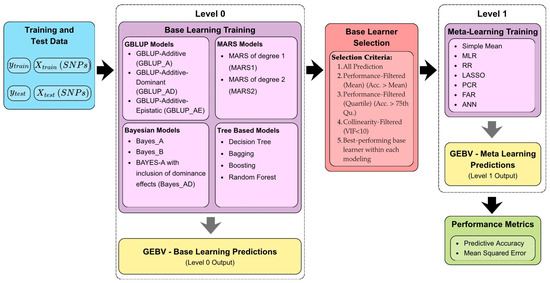
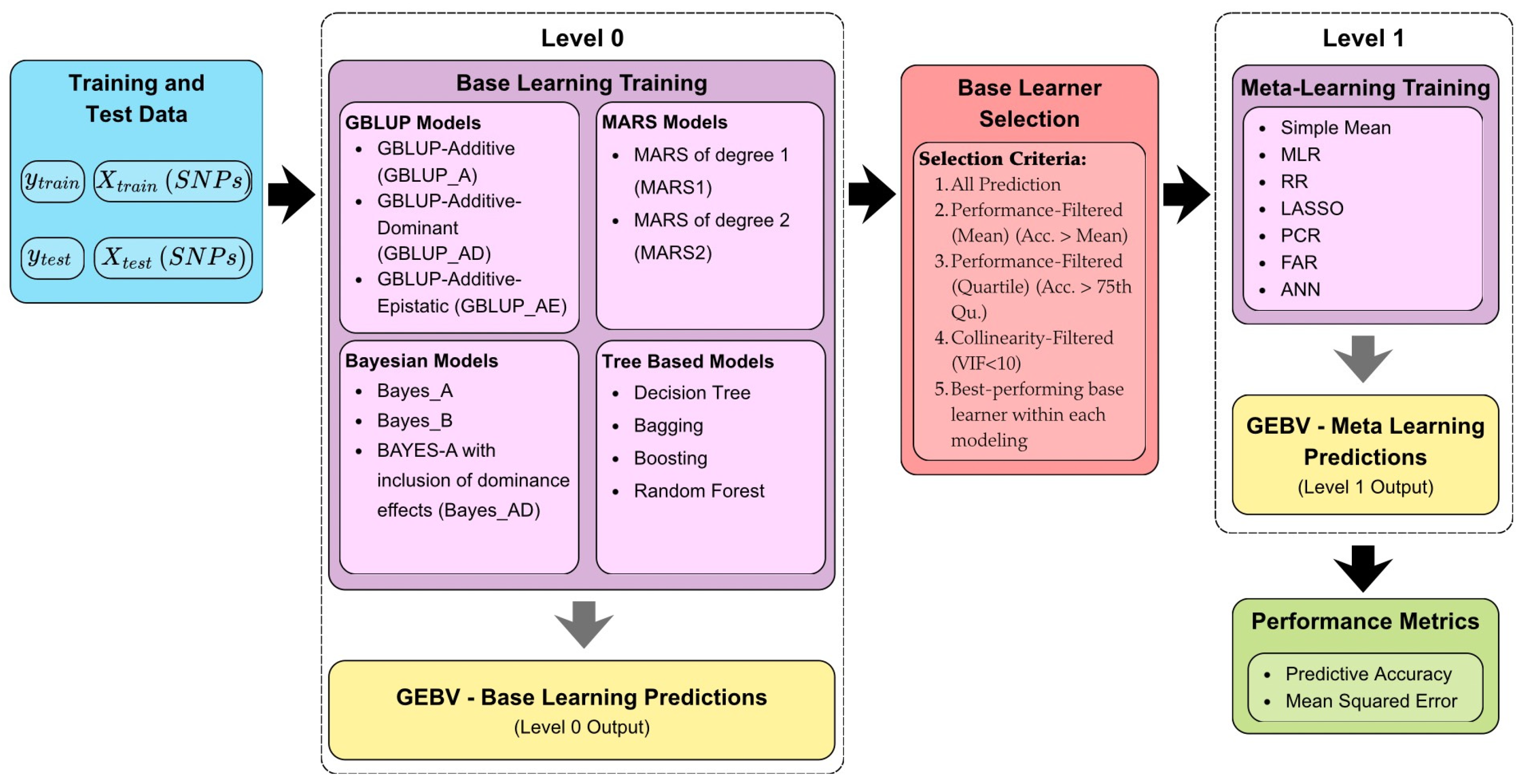
This research employs Stacked Ensemble Learning (SEL) as a strategy to enhance the accuracy of genomic predictions. The SEL approach works through a two-level hierarchy. Initially, at Level 0, multiple individual models, referred to as base learners, are trained to generate primary predictions. Subsequently, at Level 1, a higher-level model, the meta-learner, is responsible for optimally combining these primary outputs, thereby yielding a final, often superior prediction. This two-layer architecture (Levels 0 and 1) constitutes the core of the SEL methodology. Specifically, the genomic estimated breeding values from base learners, detailed in Section 2.2 (GEBV-BL), serve as the metadata (input features) for the Level 1 meta-learner. The meta-learner, detailed posteriorly, is then trained using these GEBV-BL predictions as inputs and the original phenotype data as the target variable. To evaluate the impact of different input feature sets on SEL performance, we explored four distinct combinations of base learner predictions (the metadata) for the meta-learner: i. All Predictions, including the predictions from all base learners, serving as the baseline configuration for comparison; ii. Performance-Filtered (Mean), including predictions only from base learners whose accuracy exceeded the average accuracy across all individual models; iii. Performance-Filtered (Quantile), focusing on the top-performing models, including predictions only from those whose accuracy exceeded the 75th quantile (the top 25% of the base models); iv. Collinearity-Filtered (VIF), aiming to control for multicollinearity by including predictions only from base learners that exhibited a Variance Inflation Factor (VIF) lower than 10; v. Model Selection, in which only the predictions from the best-performing base learner within each modeling class were used to train the meta-learner. The SEL scheme for genomic prediction is illustrated in Figure 1.

Figure 1. The stacked ensemble learning framework for genomic prediction. The base learners utilized at Level 0 include the following: Additive GBLUP (GBLUP_A), Additive–Dominant GBLUP (GBLUP_AD), Additive–Epistatic GBLUP (GBLUP_AE), multivariate adaptive regression splines of degree 1 (MARS1), MARS of degree 2 (MARS2), BayesA (BAYES_A), BayesB (BAYES_B), BAYES A with the inclusion of dominance effects (Bayes_AD), regression tree (RT), bagging (BAG), boosting, random forest (RF), multiple linear regression (MLR), ridge regression (RR), Least Absolute Shrinkage and Selection Operator (LASSO), principal component regression (PCR), factor regression (FAR), artificial neural network (ANN), and the arithmetic mean of the base learners’ predictions (Simple Mean).

2.3.1. Meta-Learners

Consider the following regression model of $y$ on $p$ predictor variables:

$${\mathit{y}}_{n\times 1}={\mathit{X}}_{n\times \left(p+1\right)}{\mathit{\beta }}_{\left(p+1\right)\times 1}+{\mathit{ϵ}}_{n\times 1},$$

where $\mathit{y}$ is the vector of response variable observation, $\mathit{X}$ is the incidence matrix of $\mathit{\beta }$, $\mathit{\beta }$ is the vector of coefficient regression, and $\mathit{ϵ}$ is the vector of residuals, where $\mathit{ϵ}~NM\left(\mathbf{0},\mathit{I}{\sigma }_e^2\right)$.

2.3.2. Ordinary Least Squares

The ordinary least squares (OLS) estimator of $\mathit{\beta }$, denoted ${\widehat{\mathit{\beta }}}_{\mathit{O}\mathit{L}\mathit{S}}$, is obtained by minimizing the residual sum of squares, that is, by minimizing the following expression:

$${\mathit{ϵ}}^T\mathit{ϵ}={\left(\mathit{y}-\mathit{\beta }\mathit{X}\right)}^T\left(\mathit{y}-\mathit{\beta }\mathit{X}\right).$$

which yields ${\widehat{\mathit{\beta }}}_{\mathit{O}\mathit{L}\mathit{S}}={\left({\mathit{X}}^T\mathit{X}\right)}^{-1}{\mathit{X}}^T\mathit{y}$.

2.3.3. Ridge Regression and LASSO

Ridge regression (RR) and LASSO are shrinkage methods that penalize the magnitude of regression coefficients. Estimates are obtained by minimizing a penalized residual sum of squares (RSS) [27].

The ridge regression (RR) estimator is obtained by solving the following penalized RSS minimization problem:

$${\widehat{\mathit{\beta }}}_{\mathit{R}\mathit{R}}=\underset{\mathit{\beta }}{\mathit{min}}\left\{\sum _{i=1}^n{\left(y_i-{\beta }_0-\sum _{j=1}^p{x}_{ij}{\beta }_j\right)}^2+\lambda \sum _{j=1}^p{\beta }_j^2\right\}=\underset{\mathit{\beta }}{\mathit{min}}\left\{SQR\left(\lambda \right)\right\},$$

where $\lambda \ge 0$ is the regularization (or complexity) parameter that controls the amount of shrinkage applied to the coefficients ${\beta }_j$. The constraint form of ridge regression involves a bound $t$, and there exists a one-to-one correspondence between $\lambda$ and $t$ [27]. Given $\lambda$, the coefficient estimates are obtained as follows: ${\widehat{\beta }}_0=\overline{\mathit{y}}$, the overall mean, and the remaining coefficients, ${\widehat{\mathit{\beta }}}_{\mathit{R}\mathit{R}}$, are estimated by ridge regression without an intercept, using centered predictor variables. Specifically let $Z_j=X_j-\overline{X_j}$, where $\overline{X_j}$ is the sample mean of the j-th predictor. The penalized RSS to be minimized is then the following:

$$RSS\left(\lambda \right)={\left(\mathit{y}-\mathit{Z}\mathit{\beta }\right)}^T\left(\mathit{y}-\mathit{Z}\mathit{\beta }\right)+\lambda {\mathit{\beta }}^T\mathit{\beta },$$

which yields ${\widehat{\mathit{\beta }}}_{\mathit{R}\mathit{R}}={\left({\mathit{Z}}^{\mathit{T}}\mathit{Z}+\mathit{\lambda }\mathit{I}\right)}^{-1}{\mathit{Z}}^T\mathit{y}$.

In contrast, for LASSO, the optimization problem is formulated as

$${\widehat{\mathit{\beta }}}_{\mathit{L}\mathit{A}\mathit{S}\mathit{S}\mathit{O}}=\underset{\mathit{\beta }}{\mathit{min}}\left\{\sum _{i=1}^n{\left(y_i-{\beta }_0-\sum _{j=1}^p{x}_{ij}{\beta }_j\right)}^2+\lambda \sum _{j=1}^p|{\beta }_j|\right\}=\underset{\mathit{\beta }}{\mathit{min}}\left\{SQR\left(\lambda \right)\right\},$$

Unlike ridge regression, LASSO does not admit a closed-form solution. In both methods, the optimal value of the regularization parameter $\lambda$ is typically selected via cross-validation, choosing the λ that minimizes the cross-validated RSS [27].

2.3.4. Principal Component Regression

From the data matrix ${\mathit{X}}_{n\times p}$, we obtain the covariance matrix $\mathit{S}$ and the correlation matrix $\mathit{R}={\mathit{D}}^{-1/2}\mathit{S}{\mathit{D}}^{-1/2}$, where ${\mathit{D}}^{-1/2}=diag\left(1/\sqrt{S_{ii}}\right)$. The $i$-th sample principal component is given by ${\mathit{Q}}_i={{\widehat{\mathit{e}}}_i}^T{\mathit{X}}_{j.}$, where ${\mathit{X}}_{j.}$ is the $j$-th row of the data matrix $\mathit{X}$. By maximizing the variance of each principal component, the corresponding scores and covariance matrix are obtained as ${\widehat{\mathit{Q}}}_j={\widehat{\mathit{P}}}^T{\mathit{X}}_{j.}$ and $\widehat{Cov}\left({\widehat{\mathit{Q}}}_j\right)=\widehat{\mathit{\Lambda }}$, where $\widehat{\mathit{P}}$ is the matrix of the unit eigenvectors of the sample covariance matrix $\mathit{S}$ and $\widehat{\mathit{\Lambda }}=diag\left({\widehat{\lambda }}_i\right)$. Fixing the first $k<p$ principal components, selected such that their cumulative proportion of explained variance is at least 70% [31], the principal component scores and their estimated covariance matrix are defined as ${\widehat{\mathit{Q}}}_j={\widehat{\mathit{P}}}_k^T{\mathit{X}}_{j.}$ and $\widehat{Cov}\left({\widehat{\mathit{Q}}}_j\right)={\widehat{\mathit{\Lambda }}}_k$, where ${\mathit{P}}_k^T$ is the matrix containing the first k unit eigenvectors of the sample covariance matrix $\mathit{S}$, and ${\widehat{\mathit{\Lambda }}}_k$ is the diagonal matrix of the corresponding first k eigenvalues.

This leads to the following principal component regression (PCR) model: ${\mathit{y}}_{n\times 1}={\widehat{\mathit{Q}}}_{n\times \left(k+1\right)}{\mathit{\beta }}_{\left(k+1\right)\times 1}+{\mathit{ϵ}}_{n\times 1},$ where $\mathit{y}$ is the vector of response variable observation, $\widehat{\mathit{Q}}$ represents the principal component scores for the first $k$ principal component, $\mathit{\beta }$ is the vector of coefficient regression, and $\mathit{ϵ}$ is the vector of residuals, where $\mathit{ϵ}~NM\left(\mathbf{0},\mathit{I}{\sigma }_e^2\right)$. The PCR estimator of the regression coefficients is then given by the ordinary least squares solution ${\widehat{\mathit{\beta }}}_{\mathit{P}\mathit{C}\mathit{R}}={\left({\widehat{\mathit{Q}}}^T\widehat{\mathit{Q}}\right)}^{-1}{\widehat{\mathit{Q}}}^T\mathit{y}$.

2.3.5. Factor Regression

Let $\mathit{x}={\left[\begin{array}{ccc}{X}_1& X_2& \begin{array}{cc}\cdots & X_p\end{array}\end{array}\right]}^T$ be a vector with mean $\mathit{\mu }$ and covariance matrix $\mathit{\Sigma }$, and let $\mathit{F}={\left[\begin{array}{ccc}{F}_1& F_2& \begin{array}{cc}\cdots & F_m\end{array}\end{array}\right]}^T$ denote a vector of $m$ common factors. The factor analysis model is expressed in matrix form as ${\mathit{x}}_{p\times 1}-{\mathit{\mu }}_{p\times 1}={\mathit{\Gamma }}_{p\times m}{\mathit{F}}_{m\times 1}+{\mathit{ϵ}}_{p\times 1},$ where the following assumptions hold: $E\left[\mathit{x}\right]=\mathit{\mu },E\left[\mathit{ϵ}\right]=E\left[\mathit{F}\right]=\mathbf{0},cov\left(\mathit{F}\right)={\mathit{I}}_{\mathit{m}},cov\left(\mathit{ϵ}\right)=\mathit{\Psi }=diag\left({\Psi }_i\right),{\Psi }_i>0,$ and $cov\left(\mathit{F},\mathit{ϵ}\right)=\mathbf{0}.$ Given a sample of size $n$, the sample covariance matrix $\mathit{S}$ admits the spectral decomposition $\mathit{S}=\widehat{\mathit{P}}{\widehat{\mathit{\Lambda }}\widehat{\mathit{P}}}^T\cong \widehat{\mathit{\Gamma }}{\widehat{\mathit{\Gamma }}}^T+\widehat{\mathit{\Psi }}$, where ${\widehat{\mathit{\Gamma }}}^T={\widehat{\mathit{P}}}_{\mathit{m}}{\widehat{\mathit{\Lambda }}}_{\mathit{m}}^{{\displaystyle \raisebox{1ex}{$1$}\!\left/ \!\raisebox{-1ex}{$2$}\right.}}and\widehat{\mathit{\Psi }}=diag\left(\mathit{S}-\widehat{\mathit{\Gamma }}{\widehat{\mathit{\Gamma }}}^T\right).$

The predictor of the factor scores obtained via Weighted Least Squares (WLS) is given by $\widehat{\mathit{F}}={\left({\widehat{\mathit{\Gamma }}}^T{\widehat{\mathit{\Psi }}}^{-1}\widehat{\mathit{\Gamma }}\right)}^{-1}{\widehat{\mathit{\Gamma }}}^T{\widehat{\mathit{\Psi }}}^{-1}\left(\mathit{x}-\mathit{\mu }\right)$, which leads to the following factor regression (FR) model: ${\mathit{y}}_{n\times 1}={\widehat{\mathit{F}}}_{n\times \left(m+1\right)}{\mathit{\beta }}_{\left(m+1\right)\times 1}+{\mathit{ϵ}}_{n\times 1},$ where $\mathit{y}$ is the vector of response variable observation, $\widehat{\mathit{Q}}$ represents the principal component scores for the first $k$ principal component, $\mathit{\beta }$ is the vector of coefficient regression, and $\mathit{ϵ}$ is the vector of residuals, where $\mathit{ϵ}~NM\left(\mathbf{0},\mathit{I}{\sigma }_e^2\right)$. The factor regression (FR) estimator of the regression coefficients is then obtained via ordinary least squares as ${\widehat{\mathit{\beta }}}_{\mathit{F}\mathit{R}}={\left({\widehat{\mathit{F}}}^T\widehat{\mathit{F}}\right)}^{-1}{\mathit{F}}^T\mathit{y}$.

2.3.6. Artificial Neural Network

Consider $X_1,\cdots ,X_p$, $p$ input variables, and a network with one hidden layer and one output. The output of the mth neuron in the first layer, given by a linear combination of the p input variables applied to the activation function $\phi \left(.\right)$, is $W_m=\phi \left(w_{0,m}{X}_0+\sum _{i=1}^p{w}_{i,m}{X}_i\right),m=1,\cdots ,M.$ Here, $M$ is the number of neurons, and $w_{i,m}$ is the synaptic weight between the $i-th$ input variable and the $m$-th neuron. The output of the ANN, $Y$, given by the linear combination of the $M$ neurons in the hidden layer applied to the activation function $\sigma \left(.\right)$, is $Y=\sigma \left(w_0^{\prime }{W}_0+\sum _{i=1}^M{W}_i{w}_i^{\prime }\right)$, where $w_i^{\prime }$ is the synaptic weight between the $i$-th neuron and the output layer of the network, and $w_0^{\prime }$ is the synaptic weight of the bias term $W_0$ [32].

2.4. Cross-Validation

The predictive accuracy (PA) of the individual base learner models and the overall Stacked Ensemble Learning (SEL) framework was assessed using a cross-validation (CV) scheme. First, the entire dataset was randomly partitioned into a training set (80% of individuals) and a testing (or validation) set (the remaining 20%). The training set was exclusively used to calibrate both the base learners and the SEL meta-learner. These calibrated models were then used to predict the genomic estimated breeding values (GEBVs) for the individuals in the testing set. This entire process of partitioning, training, and predicting was replicated ten times. The reported performance for each prediction approach was calculated as the average PA across these 10 replicates as further iterations yielded no substantial changes in predictive accuracy. Then, for each approach, the average PA across replicated was computed. PA was computed as the Pearson correlation coefficient between the predicted GEBVs and the adjusted phenotype values. In addition to PA, we calculated the Standard Error (SE) of the mean PA.

3. Results

Predictive Accuracy of Base Learners and Ensemble Methods

Predictive accuracy values ranged from 0.161 to 0.479 in Scenario 1, −0.016 to 0.220 in Scenario 2, 0.308 to 0.577 in Scenario 3, 0.047 to 0.240 in Scenario 4, 0.227 to 0.438 in Scenario 5, −0.040 to 0.176 in Scenario 6, −0.092 to 0.231 in Scenario 7, −0.022 to 0.093 in Scenario 8, 0.034 to 0.303 in Scenario 9, and 0.059 to 0.247 in Scenario 10 (Supplementary Table S1). Across all scenarios, the stacking ensemble methods exhibited predictive ability equal to or greater than that of the individual base learners (Supplementary Table S1).

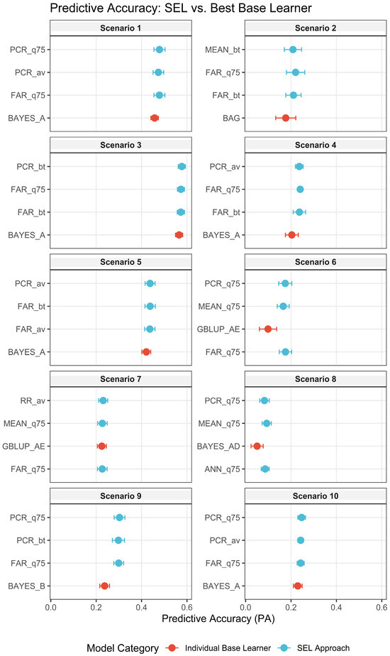
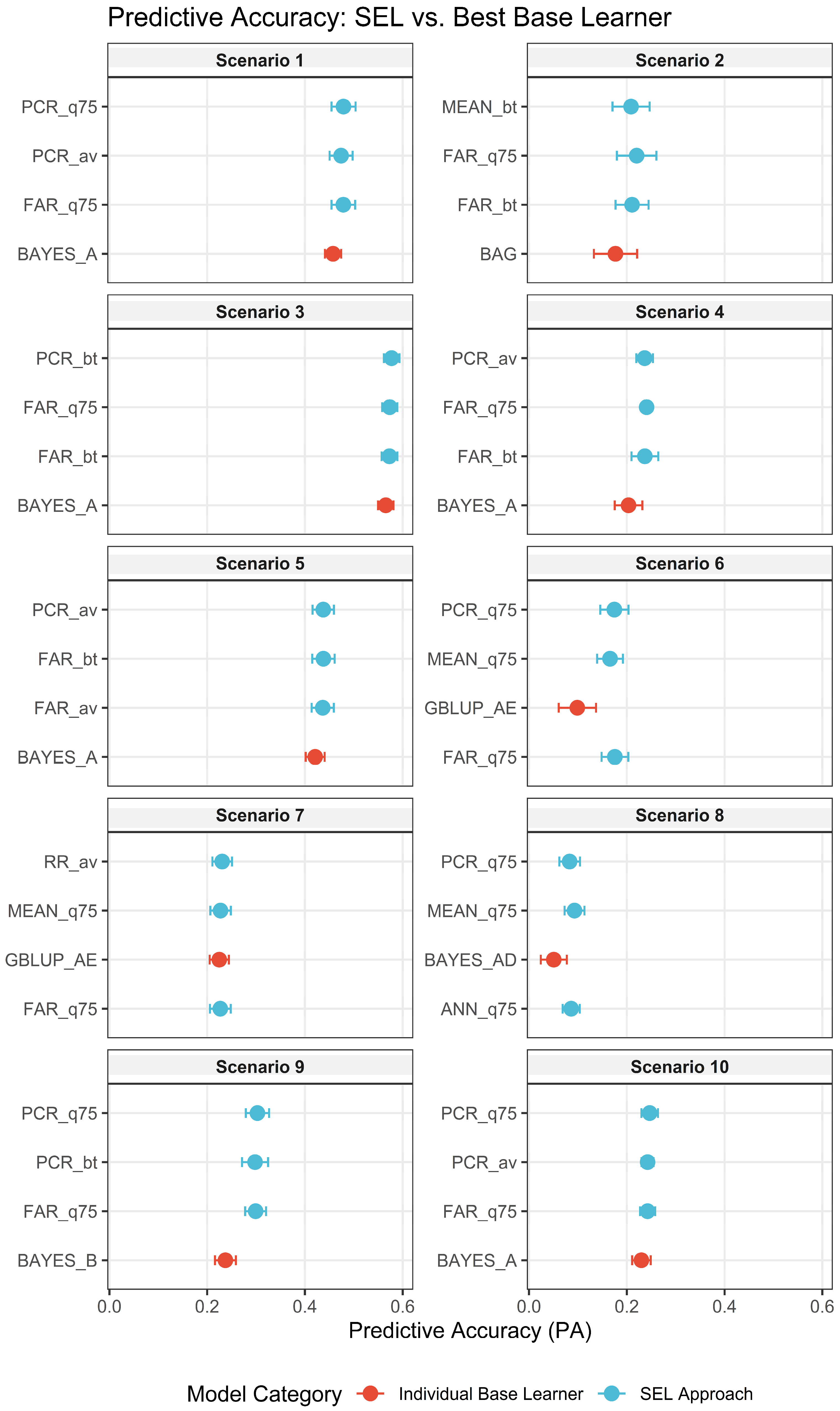
Figure 2 summarizes the performance of PA and the respective SE bar, presenting only the three best results obtained by the SEL configurations alongside the best result achieved by the single base learner, for each scenario.

Figure 2. The top three predictive accuracy results among the stacking ensemble methods and the best predictive accuracy achieved by any individual base learner. PCR_q75: Principal Component Regression (PCR)—Performance-Filtered (75th Quantile); PCR_av: PCR—Performance-Filtered (Mean); PCR_bt: PCR—Used in the Model Selection (Base Training Set); FAR_q75: Factor Regression (FAR)—Performance-Filtered (75th Quantile); FAR_av: FAR—Performance-Filtered (Mean); FAR_bt: FAR—Used in the Model Selection (Base Training Set); Mean_q75: Mean of Base Learner Predictions—Performance-Filtered (75th Quantile); Mean_av: Mean of Base Learner Predictions—Performance-Filtered (Mean); Mean_bt: Mean of Base Learner Predictions—Used in the Model Selection (Base Training Set); RR_av: Ridge Regression—Performance-Filtered (Mean); ANN_q75: Artificial Neural Network—Performance-Filtered (75th Quantile); GBLUP_AE: GBLUP Additive–Epistatic; Bayes_AD: BayesA Considering Dominance.

Typically, scenarios with 10 QTLs and a heritability of 0.6 exhibit higher predictive accuracy compared to scenarios with the same genetic effect but a polygenic architecture (100 QTLs) and lower heritability (0.3) (Figure 2).

The preliminary selection of base learner predictions proved to be a more effective strategy, exhibiting higher predictive accuracy. Indeed, stacking ensembles without such selection did not rank among the top three performers in any of the evaluated scenarios (Figure 2). Moreover, the meta-learners trained using base learner predictions filtered by Variance Inflation Factor (VIF) did not rank among the top three models in any of the evaluated scenarios (Figure 2).

In terms of methods, meta-learners based on principal component regression (PCR) and factor regression (FR) are consistently among the top three stacking ensemble learning models (Figure 2).

Table 2 shows the maximum percentage increase in predictive accuracy observed by stacking ensemble methods compared to the best base learner. Stacking ensembles show the largest relative gains in scenarios with low heritability and a greater number of QTLs while aggregating information from different models to predict a trait. Specifically, the best result showed an increase of 82.76% ($h^2=0.3,n_{QTL}=100$ and $gmd=0.8$) in predictive accuracy (Table 2). In contrast, for scenarios with greater heritability ${(h}^2=0.6)$, the greatest gain (27.59%) was observed when the genetic architecture of the trait showed epistatic effects (Table 2).

Table 2. Maximum percentage increase in predictive accuracy observed by stacking ensemble methods compared to best base learner in each evaluated scenario.

Effect	${\mathit{h}}^2 = 0.6; {\mathit{n}}_{\mathit{Q}\mathit{T}\mathit{L}} = 10$	${\mathit{h}}^2 = 0.3; {\mathit{n}}_{\mathit{Q}\mathit{T}\mathit{L}} = 100$
Additive	4.69%	24.41%
Dominance (mdd = 0.2)	2.12%	18.17%
Dominance (mdd = 0.5)	4.01%	77.5%
Dominance (mdd = 0.8)	2.63%	82.76%
Epistasis	27.59%	7.37%

Legend: Mean degree of dominance (mdd).

Supplementary Figures S1–S10 show the average correlation between predictions from base learners and those with simulated phenotypes. Notably, the correlations are higher within each method class (e.g., Genomic Best Linear Unbiased Predictor—GBLUP; multivariate adaptive regression splines—MARS; Bayesian methods; and tree-based models). These results suggest that models within the same class have similar predictions and consequently lead to the problem of multicollinearity. Therefore, selecting models to compose the meta-learners of the stacking ensemble learning presents itself as an interesting strategy (Figure 2).

To verify which base learning composed the best stacking ensembles, models with predictive accuracy above the average of all base models were filtered. Then, for this group, the mode of the number of model classes used and the most recurrent model class were obtained (Table 3). In general, the methods selected to compose the base learning of the stacking ensemble belonged to three or even four classes of models used (Table 3).

Table 3. The mode of the number of modeling classes included in the selection based on predictive accuracy exceeding the mean, with the most frequently occurring modeling classes indicated in parentheses.

Effect	${\mathit{h}}^2 = 0.6; {\mathit{n}}_{\mathit{Q}\mathit{T}\mathit{L}} = 10$	${\mathit{h}}^2 = 0.3; {\mathit{n}}_{\mathit{Q}\mathit{T}\mathit{L}} = 100$
Additive	3 (Bayesian, tree-based, and MARS)	3 (Bayesian, tree-based, and GBLUP)
Dominance (mdd = 0.2)	3 (Bayesian, tree-based, and MARS)	3 (Bayesian, tree-based, and GBLUP)
Dominance (mdd = 0.5)	2 (Bayesian and tree-based)	4 (Bayesian, tree-based, MARS, and GBLUP)
Dominance (mdd = 0.8)	3 (Bayesian, tree-based, and GBLUP)	3 (Bayesian, tree-based, and MARS)
Epistasis	3 (Bayesian, tree-based, and GBLUP)	3 (Bayesian, tree-based, and MARS)

Legend: Mean degree of dominance (mdd), Genomic Best Linear Unbiased Predictor (GBLUP), and multivariate adaptive regression splines (MARS).

The lowest Mean Squared Error (MSE) values were achieved by stacking ensemble learning in most of the evaluated scenarios (Supplementary Table S2). When a base learner achieves the lowest MSE, the maximum difference observed is 0.13 (Scenario 10: epistatic effects with h² = 0.3 and nQTL = 100).

4. Discussion

In this study, we evaluated the performance of different stacking ensemble learning configurations for the genomic prediction of complex traits. The results were compared with those from methods traditionally used in genomic selection. Ten distinct simulated phenotypic traits, considering different genetic architectures, were used. A 5-fold cross-validation scheme was employed to assess the comparison measures.

In general, stacking ensemble learning showed greater or equal predictive accuracy compared to base learning (Table S1). Base learners can perform well when their underlying assumptions match the simulated genetic architecture, but Stacked Ensemble Learning (SEL) presented robust, consistent, and reliable performance even when the true genetic model is unknown or incorrectly specified. This increase in predictive accuracy is also reported in the literature [33,34], as SEL integrates the strengths of each base learning to improve prediction [33,34,35] to generate more robust and flexible models, providing more stable predictions [36]. For genomic prediction, stacking ensemble learning can better exploit the relationships between variables and more reliably identify the genetic subtle of the evaluated traits [20,21,22,37].

As expected, factors such as heritability and the number of QTLs affect the value of predictive accuracy, where traits with higher heritability present higher predictive accuracy values [38,39]. Regarding the number of QTLs, ref. [40] highlights that a high number of QTLs increases the chances that one marker will explain the same variation as another, in genetic terms, and environmental effects, thus affecting accuracy.

Stacking ensemble learning shows a more considerable improvement in predictive ability in scenarios with low heritability and a greater number of QTLs (Table 2) as they aggregate information from different models to predict a trait. Traits with low heritability represent a greater challenge for genomic prediction [10,41].

Therefore, the application of more elaborate methods, such as stacking ensemble learning, is interesting for capturing the complexity of genetic interactions, overcoming the limitations of traditional methods in scenarios of lower heritability [39,42].

In contrast, in scenarios where genetic architecture was simulated considering epistatic effects, stacking ensemble learning showed better results when the trait had higher heritability and fewer QTLs. This is because in traits with fewer QTLs, epistasis is more pronounced, while in quantitative traits, epistasis can be diluted, playing an underlying role, since most genetic variation is additive [43]. Ref. [44] observed an increase in the accuracy of stacking ensemble learning as non-additive effects increased. However, even in scenarios where the gains with stacking ensemble learning were not as significant, the improvement was comparable to the results of [20], representing a considerable gain for perennial crops or animal breeding programs.

It should be noted that the highest predictive accuracy values were obtained by stacking ensemble learning with the prior selection of base learners (Figure 2 and Supplementary Table S1). In all scenarios, the best stacking ensemble learning used base learners with predictive accuracy above the average or above the 75th quartile of the individual distribution. These findings are consistent with [22], which also reported better performance when restricting meta-learning to the most informative models.

Among the meta-learners, principal component regression (PCR) and factor regression (FR) showed the best results (Figure 2). This may be due to the presence of multicollinearity among the values predicted by the base learners (Supplementary Figures S1–S10). According to [45], PCR is an alternative to factor analysis in the presence of multicollinearity, and FR can circumvent the problem by filtering highly correlated variables. Although the filtering in this study (selection by performance) differs from that discussed by [45], it had the direct consequence of reducing multicollinearity, favoring the performance of PCR and FR. These results also explain why linear regression, despite being listed as a common meta-learning method [20,35], did not perform well, given its sensitivity to multicollinearity. In contrast, statistical learning and machine learning methods that better handle this condition proved to be more interesting alternatives, which is consistent with what was described by [21,22].

The base learners of the selected models were generally composed of at least one method from each class (GBLUPs, MARS, Bayesian, and tree-based) (Table 3). In practice, this approach combines methods with diverse, different, and complementary characteristics, facilitating a better explanation of the relationships between variables and, consequently, a more accurate selection of individuals for improvement.

Our results show that Stacking Ensemble Learning (SEL) is a promising approach for genomic prediction, surpassing the predictive accuracy (PA) of all baseline learners, including GBLUP. It is important to highlight that this study focused on demonstrating the power of the SEL approach, which combines several models to enhance predictive accuracy. Therefore, we did not exhaustively evaluate the individual complexity of each algorithm, such as by performing an extensive hyperparameter search (e.g., the number of hidden layers in the neural network). Instead, the emphasis was placed on the synergy of the ensemble rather than the isolated performance of its components, once the strength of SEL lies in its ability to combine multiple methods, exploiting complex relationships and overcoming the limitations of individual models. However, SEL presents challenges, mainly high computational cost and hyperparameter optimization, in contrast to the efficiency of GBLUP [22]. Additionally, given that our study evaluated additive, dominance, and epistatic effects through separate scenarios, future research should explore the simultaneous integration of these components to further capture the full complexity of certain genetic architectures.

5. Conclusions

The stacking ensemble learning approach demonstrated greater predictive accuracy in all scenarios (additive, additive–dominant, and additive–epistatic). For scenarios with a higher number of QTLs (100) and lower heritability (0.3), the gain over the best individual method was up to 83%. The method also stood out in genetic architectures with fewer QTLs (10), higher heritability (0.6), and the presence of epistasis, where the percentage gain was up to 27.59%. The success of stacking ensemble learning depended on two key strategies: (1) the selection of base learners and (2) the use of robust meta-learners (such as principal component regression or regression with penalty) that effectively circumvented multicollinearity among the base predictions. The implementation of principal component regression (PCR) and Factor Analysis Regression (FAR) as meta-learners, utilizing the GEBVs from the top 25% of base models, represents a promising approach for evaluation within Selective Ensemble Learning (SEL) frameworks. Overall, this study confirms the potential of stacking but emphasizes that the final performance is dependent on the specific combination of base learners and meta-learners used. Additionally, refinements in specific hyperparameters, for example, the neural network depth, may yield additional gains.

References

- Meuwissen, T.H.E.; Hayes, B.J.; Goddard, M.E. Prediction of total genetic value using genome-wide dense marker maps. Genetics 2001, 157, 1819–1829. [Google Scholar] [CrossRef] [Scilit]
- Daetwyler, H.D.; Calus, M.P.L.; Pong-Wong, R.; de los Campos, G.; Hickey, J.M. Genomic prediction in animals and plants: Simulation of data, validation, reporting, and benchmarking. Genetics 2013, 193, 347–365. [Google Scholar] [CrossRef] [Scilit] [PubMed]
- Voss-Fels, K.P.; Cooper, M.; Hayes, B.J. Accelerating crop genetic gains with genomic selection. Theor. Appl. Genet. 2019, 132, 875–891. [Google Scholar] [CrossRef] [Scilit]
- Hickey, L.T.; Hafeez, A.N.; Robinson, H.; Jackson, S.A.; Leal-Bertioli, S.C.M.; Tester, M.; Gao, C.; Godwin, I.D.; Hayes, B.J.; Wulff, B.B.H. Breeding crops to feed 10 billion. Nat. Biotechnol. 2019, 37, 744–754. [Google Scholar] [CrossRef] [Scilit]
- Hernandez, C.O.; Wyatt, L.E.; Mazourek, M.R. Genomic prediction and selection for fruit traits in winter squash. G3 Genes Genomes Genet. 2020, 10, 3373–3383. [Google Scholar] [CrossRef] [Scilit]
- Henderson, C.R. Best linear unbiased prediction of nonadditive genetic merits in noninbred populations. J. Anim. Sci. 1985, 60, 111–119. [Google Scholar] [CrossRef] [Scilit]
- Wang, X.; Xu, Y.; Hu, Z.; Xu, C. Genomic selection methods for crop improvement: Current status and prospects. Crop J. 2018, 6, 333–340. [Google Scholar] [CrossRef] [Scilit]
- González-Camacho, J.M.; Ornella, L.; Pérez-Rodríguez, P.; Gianola, D.; Dreisigacker, S.; Crossa, J. Applications of machine learning methods to genomic selection in breeding wheat for rust resistance. Plant Genome 2018, 11, 170104. [Google Scholar] [CrossRef] [Scilit]
- Rosado, R.D.S.; Penso, G.A.; Serafini, G.A.D.; dos Santos, C.E.M.; Picoli, E.A.d.T.; Cruz, C.D.; Barreto, C.A.V.; Nascimento, M.; Cecon, P.R. Artificial neural network as an alternative for peach fruit mass prediction by non-destructive method. Sci. Hortic. 2022, 299, 111014. [Google Scholar] [CrossRef] [Scilit]
- Crossa, J.; Pérez, P.; Hickey, J.; Burgueño, J.; Ornella, L.; Cerón-Rojas, J.; Zhang, X.; Dreisigacker, S.; Babu, R.; Li, Y.; et al. Genomic prediction in CIMMYT maize and wheat breeding programs. Heredity 2014, 112, 48–60. [Google Scholar] [CrossRef] [Scilit]
- Bayer, P.E.; Petereit, J.; Danilevicz, M.F.; Anderson, R.; Batley, J.; Edwards, D. The application of pangenomics and machine learning in genomic selection in plants. Plant Genome 2021, 14, e20112. [Google Scholar] [CrossRef] [Scilit]
- Jannink, J.L.; Lorenz, A.J.; Iwata, H. Genomic selection in plant breeding: From theory to practice. Brief. Funct. Genom. 2010, 9, 166–177. [Google Scholar] [CrossRef] [Scilit]
- Azodi, C.B.; Bolger, E.; McCarren, A.; Roantree, M.; de los Campos, G.; Shiu, S.-H. Benchmarking parametric and machine learning models for genomic prediction of complex traits. G3 Genes Genomes Genet. 2019, 9, 3769–3780. [Google Scholar] [CrossRef] [Scilit]
- Mendes-Moreira, J.; Soares, C.; Jorge, A.M.; De Sousa, J.F. Ensemble approaches for regression: A survey. ACM Comput. Surv. 2012, 45, 1–40. [Google Scholar] [CrossRef] [Scilit]
- Dietterich, T.G. Ensemble methods in machine learning. In Proceedings of the International Workshop on Multiple Classifier Systems, Cagliari, Italy, 9–11 June 2000; Springer: Heidelberg/Berlin, Germany, 2000; pp. 1–15. [Google Scholar] [CrossRef] [Scilit]
- Ardabili, S.; Mosavi, A.; Várkonyi-Kóczy, A.R. Advances in machine learning modeling reviewing hybrid and ensemble methods. In Proceedings of the International Conference on Global Research and Education, Budapest, Hungary, 4–7 September 2019; Springer: Cham, Switzerland, 2020; pp. 215–227. [Google Scholar] [CrossRef] [Scilit]
- Sousa, I.C.d.; Nascimento, M.; Silva, G.N.; Nascimento, A.C.C.; Cruz, C.D.; Silva, F.F.; Almeida, D.P.d.; Pestana, K.N.; Azevedo, C.F.; Zambolim, L.; et al. Genomic prediction of leaf rust resistance to Arabica coffee using machine learning algorithms. Sci. Agric. 2021, 78, e20200021. [Google Scholar] [CrossRef] [Scilit]
- Wolpert, D.H. Stacked generalization. Neural Netw. 1992, 5, 241–259. [Google Scholar] [CrossRef] [Scilit]
- Li, W.; Fang, Z.; Wang, Y. Stacking ensemble of deep learning methods for landslide susceptibility mapping in the Three Gorges Reservoir area, China. Stoch. Environ. Res. Risk Assess. 2022, 36, 2235–2254. [Google Scholar] [CrossRef] [Scilit]
- Liang, M.; Chang, T.; An, B.; Duan, X.; Du, L.; Wang, X.; Miao, J.; Xu, L.; Gao, X.; Zhang, L.; et al. A stacking ensemble learning framework for genomic pre-diction. Front. Genet. 2021, 12, 600040. [Google Scholar] [CrossRef] [Scilit] [PubMed]
- Mota, L.F.; Giannuzzi, D.; Bisutti, V.; Pegolo, S.; Trevisi, E.; Schiavon, S.; Gallo, L.; Fineboym, D.; Katz, G.; Cecchinato, A. Real-time milk analysis integrated with stacking ensemble learning as a tool for the daily prediction of cheese-making traits in Holstein cattle. J. Dairy Sci. 2022, 105, 4141–4155. [Google Scholar] [CrossRef] [Scilit]
- Nascimento, M.; Nascimento, A.C.C.; Azevedo, C.F.; Oliveira, A.C.B.; Caixeta, E.T.; Jarquin, D. Enhancing genomic prediction with stacking ensemble learning in Arabica coffee. Front. Plant Sci. 2024, 15, 1373318. [Google Scholar] [CrossRef] [Scilit] [PubMed]
- R Core Team. R: A Language and Environment for Statistical Computing; R Foundation for Statistical Computing: Vienna, Austria, 2025. [Google Scholar]
- Gaynor, R.C.; Gorjanc, G.; Hickey, J.M. AlphaSimR: An R package for breeding program simulations. G3 Gene Genomes Genet. 2021, 11, jkaa017. [Google Scholar] [CrossRef] [Scilit]
- Covarrubias-Pazaran, G. Genome-assisted prediction of quantitative traits using the r package sommer. PLoS ONE 2016, 11, e0156744. [Google Scholar] [CrossRef] [Scilit]
- Friedman, J.H. Multivariate adaptive regression splines (with discussion). Ann. Stat. 1991, 19, 1–67. [Google Scholar] [CrossRef] [Scilit]
- Hastie, T.; Tibshirani, R.; Friedman, J. The Elements of Statiscal Learning: Data Mining, Inference, and Prediction, 2nd ed.; Springer: New York, NY, USA, 2008; 745p. [Google Scholar]
- Milborrow, S. Notes on the Earth Package. Available online: http://www.milbo.org/doc/earth-notes.pdf (accessed on 6 October 2024).
- Wittenburg, D.; Melzer, N.; Reinsch, N. Including non-additive genetic effects in Bayesian methods for the prediction of genetic values based on genome-wide markers. BMC Genet. 2011, 12, 74. [Google Scholar] [CrossRef] [Scilit]
- Morgan, J.N.; Sonquist, J.A. Problems in the analysis of survey data, and a proposal. J. Am. Stat. Assoc. 1963, 58, 415–434. [Google Scholar] [CrossRef]
- Ferreira, D.F. Estatística Multivariada, 3rd ed.; Editora UFLA: Lavras, Brazil, 2018. [Google Scholar]
- Cruz, C.D.; Nascimento, M. Inteligência Computacional Aplicada ao Melhoramento Genético; Editora UFV: Viçosa, Brazil, 2018; 414p. [Google Scholar]
- Gu, L.L.; Yang, R.Q.; Wang, Z.Y.; Jiang, D.; Fang, M. Ensemble learning for integrative prediction of genetic values with genomic variants. BMC Bioinform. 2024, 25, 103. [Google Scholar] [CrossRef] [Scilit]
- Mahajan, P.; Uddin, S.; Hajati, F.; Moni, M.A. Ensemble learning for disease prediction: A review. Healthcare 2023, 11, 1808. [Google Scholar] [CrossRef] [Scilit] [PubMed]
- Mienye, I.I.; Sun, Y. A survey of ensemble learning: Concepts, algorithms, applications, and prospects. IEEE Access 2022, 10, 99129–99149. [Google Scholar] [CrossRef] [Scilit]
- Ghasemieh, A.; Lloyed, A.; Bahrami, P.; Vajar, P.; Kashef, R. A novel machine learning model with stacking ensemble learner for predicting emergency readmission of heart-disease patients. Decis. Anal. J. 2023, 7, 100242. [Google Scholar] [CrossRef] [Scilit]
- Mohammed, A.; Kora, R. A comprehensive review on ensemble deep learning: Opportunities and challenges. J. King Saud Univ.-Comput. Inf. Sci. 2023, 35, 757–774. [Google Scholar] [CrossRef] [Scilit]
- Gunundu, R.; Shimelis, H.; Mashilo, J. Genomic selection and enablers for agronomic traits in maize (Zea mays): A review. Plant Breed. 2023, 142, 573–593. [Google Scholar] [CrossRef] [Scilit]
- Kaler, A.S.; Purcell, L.C.; Beissinger, T.; Gillman, J.D. Genomic prediction models for traits differing in heritability for soybean, rice, and maize. BMC Plant Biol. 2022, 22, 87. [Google Scholar] [CrossRef] [Scilit]
- Costa, W.G.; Celeri, M.O.; de Paiva Barbosa, I.; Silva, G.N.; Azevedo, C.F.; Borem, A.; Nascimento, M.; Cruz, C.D. Genomic prediction through machine learning and neural networks for traits with epistasis. Comput. Struct. Biotechnol. J. 2022, 20, 5163–5172. [Google Scholar] [CrossRef] [Scilit]
- Combs, E.; Bernardo, R. Accuracy of genomewide selection for different traits with constant population size, heritability, and number of markers. Plant Genome 2013, 6, 1–7. [Google Scholar] [CrossRef] [Scilit]
- Vieira, R.A.; Nogueira, A.P.O.; Fritsche-Neto, R. Optimizing the selection of quantitative traits in plant breeding using simulation. Front. Plant Sci. 2025, 16, 1495662. [Google Scholar] [CrossRef] [Scilit]
- Mackay, T.F. Q&A: Genetic Analysis of Quantitative Traits. J. Biol. 2009, 8, 23. [Google Scholar] [CrossRef] [Scilit]
- Mota, L.F.; Giannuzzi, D.; Pegolo, S.; Sturaro, E.; Gianola, D.; Negrini, R.; Trevisi, E.; Marsan, P.A.; Cecchinato, A. Genomic prediction of blood biomarkers of metabolic disorders in Holstein cattle using parametric and nonparametric models. Genet. Sel. Evol. 2024, 56, 31. [Google Scholar] [CrossRef] [Scilit] [PubMed]
- Kyriazos, T.; Poga, M. Dealing with multicollinearity in factor analysis: The problem, detections, and solutions. Open J. Stat. 2023, 13, 404–424. [Google Scholar] [CrossRef]
Disclaimer/Publisher’s Note: The statements, opinions and data contained in all publications are solely those of the individual author(s) and contributor(s) and not of MDPI and/or the editor(s). MDPI and/or the editor(s) disclaim responsibility for any injury to people or property resulting from any ideas, methods, instructions or products referred to in the content. |
© 2026 by the authors. Licensee MDPI, Basel, Switzerland. This article is an open access article distributed under the terms and conditions of the Creative Commons Attribution (CC BY) license.