


Abstract
Soil heavy metal pollution poses a threat to agricultural sustainability, food safety, and human health. The ecologically fragile Yellow River Basin is a critical hub for agriculture, energy, and mining; however, soil heavy metal studies remain fragmented, and basin-wide syntheses are limited almost entirely to agricultural soils. This study presents a basin-wide analysis of As, Cd, Cr, Cu, Ni, Pb, and Zn in topsoil, based on 2498 sampling locations compiled from 347 publications, using an integrated framework of receptor modeling, multivariate spatial statistics, self-organizing maps, and probabilistic human health and ecological risk assessment. Four pollution sources, namely agricultural–industrial, emissions, mining–smelting, and geogenic/lithogenic, were resolved. Agriculture–industry and emissions posed considerable ecological risks (mean PER = 367.9 and 353.4), with Cd and Pb accounting for 95.7% of the risk. The non-carcinogenic hazard was negligible for adults, but 8.6% of sites exceeded the safe threshold for children, and the carcinogenic risk surpassed 10−6 for all groups, with 2.6–9.6% of sites exceeding 10−4. Spatially, the strongest multimetal contamination corridors are the Baiyin–Lanzhou corridor (upper–middle reaches) for Cu-Pb-Zn (mining–smelting) and the Xi’an–Weinan belt (middle reaches) for Cd-Pb (agricultural–industrial and emissions). Multivariate clustering was more extensive (56.1% of sites) than single-metal clustering (13.1–26.2%), confirming coherent source-linked zones. Ecological risks were driven by Cd and Pb, whereas human health risks were driven by As, Cr, and Ni. This divergence and the strong spatial organization of the risk clusters highlight the need for source-specific, spatially targeted mitigation, which requires monitoring across all land use types. The compiled dataset, although extensive, is constrained by heterogeneity in sampling periods and analytical methods and by sparse coverage in some grassland, desert, and plateau regions.
1. Introduction
Heavy metal pollution in soils is a global environmental concern, threatening ecosystem sustainability, food safety, and human health [1]. Heavy metals are non-degradable, accumulate in the soil matrix, persist for decades, impair soil function, and can be released into the environment, contaminating the food web and causing chronic toxicity [2]. Large river basins are particularly vulnerable because they support intensive agriculture, dense populations, and diverse industries and contain extensive mineral resources [3], while also acting as both sources and sinks for pollutants [4].
The Yellow River Basin is strategically important yet environmentally vulnerable, covering a drainage area of 795,000 km2. It encompasses 15% of China’s croplands, supplies water to 160 million people, and contains substantial mineral and energy resources [5,6]. The basin spans highly diverse physiographic settings: the upper reaches traverse the Qinghai–Tibet Plateau and the Inner Mongolian grasslands; the middle reaches cut through the thick Quaternary deposits of the Loess Plateau; and the lower reaches spread across the alluvial North China Plains [7]. This geological and climatic diversity gives rise to a mosaic of soil types (Cambisols, Luvisols, Anthrosols, etc.), each with different pH values, organic matter content, and metal retention capacities [4,5]. The Yellow River is the most heavily sediment-laden in the world [8], and human activities such as intensive agriculture, coal mining, non-ferrous metal smelting, and manufacturing further increase its vulnerability to pollution [9,10]. These natural geochemical backgrounds and anthropogenic inputs have turned this basin into a hotspot of heavy metal pollution, with levels frequently exceeding regulatory thresholds in soils [5,6,11], sediments [4,8,12], and crops [13,14,15].
Site-specific studies have documented heavy metal concentrations exceeding local background values and regulatory thresholds in several regions: the industrial corridor of Baiyin shows enrichments in Cd, Pb, Cu, and Zn [16,17]; the Baotou and Jiyuan areas are linked with Hg and Pb anomalies [18,19]; and the agricultural areas of Weinan and Luoyang exhibit Cd and Hg contamination [4,20]. However, these investigations provide a fragmented picture that is insufficient for basin-wide environmental management. A few basin-scale analyses have been attempted, but they have focused exclusively on agricultural soils [5,11], ignoring large areas of grassland, forests, deserts (e.g., Kubuqi, Mu Us), mining and industrial zones, and urban agglomerations [9,10]. Different land cover types exhibit distinct geochemical backgrounds and pollution pressures [2,21]. For example, grasslands and forests receive long-range atmospheric deposition [6,22], mining areas generate local anomalies [23], and urban soils accumulate metals from traffic, construction, and waste disposal [18]. Therefore, ignoring non-agricultural soils leaves the full spectrum of contamination, its spatial extent, and the associated ecological and health risks poorly characterized.
The present study addresses these gaps by integrating spatial statistics with receptor modeling and probabilistic risk analysis applied to a dataset of 2498 locations from major land cover types in the Yellow River Basin. The analysis focuses on seven heavy metals: As, Cd, Cr, Cu, Ni, Pb, and Zn. Univariate spatial clusters were detected using the global and local Moran’s I [24,25]; multivariate metal signatures were assessed with the local Geary’s C [26]; and multimetal pollution patterns were identified via self-organizing maps [27]. Source apportionment was performed using the Positive Matrix Factorization (PMF) model [28], followed by potential ecological risk [29] and probabilistic Monte Carlo health risk assessments [30,31]. The objectives of this study were (1) to quantitatively apportion natural and anthropogenic sources of heavy metals in topsoils; (2) to characterize the spatial distribution, clustering, and autocorrelation patterns of these metals; and (3) to evaluate source-specific ecological, non-carcinogenic, and carcinogenic health risks. This approach provides a baseline for spatially targeted pollution management and demonstrates the value of integrating multivariate spatial statistics, receptor modeling, and probabilistic risk assessment for large-scale environmental forensics.
2. Materials and Methods
2.1. Study Area
The Yellow River is known as the cradle of Chinese civilization. It is the second-longest river in China, after the Yangtze River, and the sixth-largest in the world. This river has historical and cultural significance and is also regarded as China’s Sorrow due to its unpredictable, catastrophic historical flooding [5]. The Yellow River is approximately 5464 km long and spans diverse landscapes along its course. Its source is located in the high-altitude headwaters of the Qinghai–Tibet Plateau. The subsequent floodplains are the erosive heartlands of the Loess and Ordos plateaus, followed by the engineered North China Plains. The passage through the Loess and Ordos plateaus causes the river to pick up sedimentary loads, and it is, therefore, considered the world’s most sediment-laden river. The Yellow River Basin spans approximately 795,000 km2. The river mouth empties into the Bohai Sea. It supports approximately 12% of China’s population and irrigates nearly 15% of its arable land [11].
The upper reaches of the river encompass the Qinghai, Gansu, Ningxia, and Inner Mongolia regions, with the major cities of Lanzhou, Xining, Yinchuan, Hohhot, Baotou, and Ordos. The middle reaches pass through Shaanxi, Shanxi, and parts of Henan Province, with major cities including Xi’an, Yulin, Yan’an, Luoyang, and Sanmenxia. The lower reaches comprise Henan and Shandong Provinces, with major population centers including Zhengzhou, Jinan, Kaifeng, Dongying, Zibo, and Tai’an. Grassland is a major land use category in the basin, followed by deserts, as the basin hosts some of China’s major deserts, including Kubuqi, Tengger, Ulan Buhe, and Mu Us (Figure S1a). Severe winds, rains, and stream interactions cause severe erosion in the region, and desertification is a major challenge. Therefore, this region is also among the pilot examples for ecological conservation and desertification prevention measures, especially green barriers and desert-crossing roads, which have significantly reduced erosion and increased vegetation [21].
The average precipitation in the basin is 454 mm, with most arid regions receiving as little as 200 mm per year, while the lower reaches average 671 mm, with most of the precipitation concentrated during the monsoon, causing severe storms and floods [8]. The climate in the river’s source region on the Qinghai–Tibet Plateau is subarctic and tundra, i.e., cold year-round with a very short growing season. The upper and middle reaches feature arid steppe and cold desert climates, i.e., semi-arid to arid, with very low and irregular rainfall. However, the middle and lower reaches feature a cold continental climate with dry winters, characterized by hot, wet summers and cold, dry winters [23]. The winter temperature averages around 0 °C, while, in summer, it is above 20 °C. The annual mean maximum and minimum temperatures in the basin are 3.24 and −31.05 °C [7].
2.2. Data Collection
Data on seven heavy metals, namely As, Cd, Cr, Cu, Ni, Pb, and Zn, in the surface soil layer were collected from the literature published between 2004 and 2026. A total of 347 publications and datasets were selected, from which georeferenced data for 2498 sampling locations were extracted. The data were projected in ArcGIS, and sampling points within the Yellow River Basin were extracted as a final dataset. The distribution of the sampling locations is shown in Figure 1c, and the publication years are shown in Figure S1b. The list of selected publications is provided in Table S9, and the data collection principles and relevant details are presented in Section S2.1.
Figure 1.
A world map showing the location of China (a), a map of China showing the Yellow River Basin (b), and the distribution of sampling points in the Yellow River Basin while provinces are highlighted in capital letters (c).
To assess whether data across publications introduced systematic bias, a sensitivity analysis was conducted using a spatial permutation test. For each heavy metal (As, Cd, Cr, Cu, Ni, Pb, Zn), the empirical variogram was computed and fitted to a theoretical spherical or exponential model. The variogram range, defined as the distance over which heavy metal concentrations are spatially correlated, was selected as the primary test statistic because it is the most sensitive indicator of spatial structure [32]. A total of 999 perturbed datasets were generated for each metal by randomly swapping heavy metal concentrations between points that were within 2 km of each other and that originated from different source studies. Points with no eligible neighbor retained their original concentration. For each perturbed dataset, the variogram range was recalculated. A two-tailed permutation p-value was computed as the proportion of permuted ranges that deviated from the mean of the permuted distribution at least as much as the original range using a significance threshold of α = 0.05. The results of the sensitivity analysis are presented in Table S1. For all heavy metals (As, Cd, Cr, Cu, Ni, Pb, Zn), no statistical evidence was found that the original range differed from the distribution of permuted ranges.
2.3. Positive Matrix Factorization (PMF) Analysis
PMF is a widely used bilinear receptor model for the source apportionment of heavy metals [28]. The model decomposes the concentration matrix into factor contributions and factor profiles , with residuals , as shown in Equation (1):
where is the concentration of the metal in a sample . is the source contribution relative to sample . is the concentration of metal in pollution source . is the residual for the metal in sample . The model minimizes the weighted sum of the squared residuals, calculated via the minimum value of the objective function (Equation (2)).
where and are the number of samples and metals, respectively; is the uncertainty associated with each observation. The uncertainties were estimated using the EPA PMF 5.0 combined-error model [33,34] using Equation (3):
where is the species-specific method detection limit, estimated as half the 5th-percentile concentration for each metal. The analytical error fraction of 10% (0.1) was used as a standard for heavy metal analysis to ensure that every observation received a unique, concentration-dependent uncertainty value (Figure S11a). indicates concentrations above , and indicates concentrations below or equal to .
For observations below or missing values, concentrations were substituted with the species-specific median concentration (Figure S11d). The associated uncertainties were inflated by a factor of four to algorithmically down-weight their influence during factor resolution, consistent with the EPA PMF 5.0 guidelines for handling missing data (Figure S11c,e). All metals passed the signal-to-noise (S/N) ratio threshold (>2), with S/N values ranging from 4.48 to 6.73, confirming their suitability for PMF analysis (Figure S11b). Model robustness was evaluated through 200-run bootstrap resampling to derive 90% confidence intervals for source contributions and profiles (Figure S11f–i). Model fit was assessed using the Q/Qexp ratio and reconstruction R2 for each metal (Figure S11j). A Q/Qexp ratio of 0.94 confirmed adequate model fit without over-factorization. Rotational stability was examined using a displacement of factor elements (DISP) analysis, in which the change in Q was evaluated under factor perturbation. The 4-factor solution was selected based on the combination of the lowest Q/Qexp ratio, interpretable factor profiles, and stability across bootstrap and DISP analyses. The distribution of the scaled residuals was symmetric, confirming the adequate model fit (Figure S11k).
2.4. Univariate Spatial Autocorrelation Analysis
The spatial structure and clustering patterns of individual heavy metal concentrations (As, Cd, Cr, Cu, Ni, Pb, Zn) were assessed using the global and local Moran’s I statistics [24,25]. Heavy metal concentrations were transformed using the Yeo–Johnson method to stabilize variance and improve the symmetry for graphical display only [35], while other inferential Moran statistics were calculated on the original heavy metal concentrations (mg/kg). A spatial weights matrix was constructed using a k = 5 nearest neighbor approach, and global Moran’s I spatial autocorrelation was measured using Equation (4) [24]:
Similarly, Local Indicators of Spatial Association (LISA)—specifically, the local Moran’s —was calculated for each location using Equation (5) [25]:
where is the number of spatial units, and are attribute values at locations and , is the mean of the attribute, is the spatial weight between and , and is the sum of all spatial weights . Meanwhile, was calculated using Equation (6):
Significance was evaluated through a conditional randomization procedure with 999 permutations, yielding a pseudo--value. Positive values indicate high clusters surrounded by high or low surrounded by low, while negative values denote spatial outliers. Significant locations were classified into quadrants, namely high–high, low–high, low–low, and high–low, following LISA interpretation [25].
2.5. Multivariate Spatial Clustering Using Local Geary’s C
The multivariate spatial clustering of heavy metals was characterized using the local Geary statistic for multivariate data [8], given in Equation (7):
where is the multivariate local Geary’s C at site , is the total number of sampling points, is the total number of heavy metals, is the concentration of heavy metal at site , is the concentration of the same metal at a neighboring site , is the global mean of metal , and are elements of a row-standardized spatial weights matrix . The weights matrix was constructed using a nearest neighbor approach. Significance testing was the same as used for univariate analysis [26].
2.6. Self-Organizing Maps (SOMs) and Hierarchical Clustering for Multivariate Patterns
An SOM was trained on the transformed data [27,35], and the SOM codebook vectors were clustered using agglomerative hierarchical clustering [36]. A similar nearest neighbor approach was used for imputation. The SOM was used to project the seven heavy metal data onto a 10 × 10 neural grid for multivariate analysis. During training, at each step, a random observation vector was presented, the best-matching unit was identified via the minimum Euclidean distance, and the prototype vectors were updated, using Equation (8):
where is the learning rate, and is a Gaussian neighborhood function centered on the winner. Training was performed on 1000 iterations with an initial learning rate of 0.5. After convergence, the 100 codebook vectors were grouped into four clusters by agglomerative hierarchical clustering using Ward’s minimum variance criterion [36]. Each sample inherited the cluster label of its best-matching neuron. Cluster centroids and spatial distributions were then inspected to characterize multivariate heavy metal assemblages.
2.7. Potential Ecological Risk Assessment (PER)
The potential ecological risk contributed by each PMF source was quantified using the classical risk index framework of Hakanson [29], described in Equation (9):
where is the measured total concentration of metal at site , is the background reference value for metal , is the toxic response factor of metal , and is the number of metals. This index was also applied to source-specific concentrations to apportion the risk from individual PMF sources, using Equation (10):
where is the factor contribution of PMF source at site , and is the loading of the metal on source , expressed in mg/kg. Meanwhile, the source-specific potential ecological risk index for source at site was calculated using Equation (11):
where is the toxic response factor for metal , is the background reference contamination for metal , and is the number of heavy metals. Similarly, the PER from individual heavy metals was also calculated. Background values of soil heavy metal concentrations are presented in Table S3. The values were classified into four risk categories: low (PER 150), moderate (150–300), considerable (300–600), and very high (600) [29].
2.8. Probabilistic Health Risk Assessment
A probabilistic human health risk assessment was performed for three receptor groups, namely adult males, adult females, and children, using a Monte Carlo framework and exposure via incidental soil ingestion and the inhalation of resuspended particles, and dermal contact was evaluated following standard USEPA models [30,31,34]. The average daily dose (ADD, mg/kg/d) for each exposure pathway was calculated using Equations (12)–(14):
where is the concentration of heavy metal in sample (mg/kg); is the soil ingestion rate (mg/d); is the inhalation rate (m3/d); is the exposure frequency (d/yr); is the exposure duration (yr); is the unit conversion factor (10−6 kg/mg); is body weight (kg), is the averaging time (d), equal to for non-cancer and for cancer; is the particle emission factor (1.36 × 10⁹ m3/kg); is the exposed skin surface area (cm2); is the soil-to-skin adherence factor (mg/cm2); and is the dermal absorption fraction of metal . Non-carcinogenic risk was expressed as the hazard index (HI) and calculated using Equation (15):
where , and is the oral reference dose of metal (mg/kg/d). An HI 1 indicates a potential non-carcinogenic concern. Similarly, carcinogenic risk was calculated as the incremental lifetime cancer risk (CR) using Equation (16):
where is the lifetime-averaged daily dose () and is the oral slope factor of heavy metal (per mg/kg/d). Thresholds of 10−6 and 10−4 were used to denote acceptable and unacceptable cancer risk levels. Moreover, the total concentrations of heavy metals were replaced by source-specific contributions to apportion the risk for PMF sources.
2.9. Monte Carlo Simulation
A two-dimensional Monte Carlo simulation was implemented, including 100,000 iterations for the ingestion-only route and 50,000 for the multi-route model to propagate parameter uncertainty and variability. Total metal concentrations were sampled from log-normal distributions fitted to the measured data by maximum likelihood. Exposure factors were drawn from the distributions listed in Table S7. The HI and CR were recalculated for each iteration, yielding empirical distributions from which probabilities of exceeding risk thresholds were derived. The influence of individual metals on the total HI and CR was examined using Spearman rank correlation coefficients (ρ) between the per-metal risk contributions and the total index, computed from a 10,000-iteration sensitivity run.
2.10. Data Analysis, Software, and Mapping
Principal component analysis (PCA) was conducted in OriginPro (Version 2024). The PCA score and loading plots, Pearson correlation analysis, and boxplots of heavy metal distributions were also generated using OriginPro. Self-organizing maps, agglomerative clustering, univariate spatial autocorrelation (global Moran’s I, LISA), and probabilistic human health risk modeling were scripted in Python (Version 3.11). The empirical variogram and multivariate local Geary’s C analysis was performed in R (Version 4.3). Maps and statistical graphs were produced using ArcGIS Pro (Version 3.2), Python, R, and OriginPro. Spatial interpolation was performed in ArcGIS using the inverse distance weighting (IDW) method. To validate the IDW interpolation, leave-one-out cross-validation (LOOCV) analysis was performed for each metal, and the optimized IDW model, using automatic parameter optimization, was compared with the default model (power = 2). The root mean square error (RMSE) and mean error (ME) were computed as the accuracy metrics (Table S8).
3. Results
3.1. Descriptive Statistics and Spatial Distribution of Heavy Metals
The concentrations of As, Cd, Cr, Cu, Ni, Pb, and Zn spanned 0.01–812.44, 0–589.1, 0.03–659, 0.05–4341, 0.39–2070, 0.01–8729.46, and 0.21–8288.58, respectively. The data showed right-tailed distributions with skewness, ranging from 2.52 for As to 18.37 for Ni. The mean values were also substantially higher than the medians for all metals; for example, the Cd mean and median were 12.96 and 0.36, respectively—that is, 36 times higher. The mean (52.41) and median (14.46) values of As were 3.6 times higher; the Pb mean (66.04) and median (24) displayed a factor of 2.8. The CV values showed high relative variability, with all exceeding 1; the highest was observed for Pb (4.91). The IQR values also showed distinct metal behaviors, ranging from 1.09 for Cd to 54.43 for Zn (Figure 2, Table S2). Pairwise Pearson correlations revealed that heavy metals were positively correlated across the basin (Figure S2a). The correlations of Cr and Cu with Ni were the strongest, followed by Cd, Cu, Pb, and Zn, and none of the metals were negatively correlated. Principal component analysis (PCA) also revealed that Ni and Cr accounted for 24.98% of the variance, and PC2 explained 18.3% of the factor loadings, with Pb, As, Cd, and Zn dominating, while Cu showed less dominance (Figure S2b).
Figure 2.
Boxplot depicting data points and normal distribution curve of heavy metals in soil, including As (a), Cd (b), Cr (c), Cu (d), Ni (e), Pb (f), and Zn (g), in the Yellow River Basin. Subplots combine a vertical scatter plot, the IQR, the median, and outliers. A fitted density curve shows the overall distribution and highlights skewness.
Figure 3 shows the spatial interpolation of heavy metals. A west–east gradient was observed, with concentrations generally higher in western and central basin areas and lower in northern–central grasslands and eastern croplands. Metal concentrations were higher around prominent mining (e.g., Baiyin and Lanzhou) and industrial (e.g., Xi’an and Taiyuan) regions. Cd and As levels were higher around croplands, while the Pb and Zn concentrations were higher around urban centers and transportation corridors. Natural background conditions were observed in regions with less anthropogenic disturbance, e.g., grassland areas in northern Inner Mongolia (Figure 3).
Figure 3.
Spatial distribution of heavy metals (mg/g), including As (a), Cd (b), Cr (c), Cu (d), Ni (e), Pb (f), and Zn (g) in the Yellow River Basin.
3.2. Source Analysis of Heavy Metals
The interpolated factor scores in the Yellow River Basin showed distinct spatial patterns (Figure 4). The Positive Matrix Factorization (PMF) decomposed the heavy metal concentrations into four latent factors. Factor 1 explained 43.3% of the total variance, followed by factor 3 (41.6%), factor 4 (11.7%), and factor 2 (1.2%; Figure S3). The factor loadings of individual metals are shown in Figure S4. Factor 1 was dominated by Zn (96.8%). It is linked to mixed anthropogenic inputs, including agricultural and industrial activities. Its spatial patterns were elevated in the central and eastern sections of the basin, particularly around Xi’an and Weinan and in some irrigated areas of Ningxia, Henan, and Taiyuan. Factor 2 was dominated by Cr (48%), Ni (37.7%), and As (10.3%), showing geogenic/lithogenic and mining influences as its spatial interpolation showed higher scores in the upper and middle reaches (western and central Gansu, Ningxia, and parts of Shanxi), dominated by grasslands. Factor 3 was dominated by Pb (95.4%), primarily linked to historical anthropogenic emissions, including industrial and coal combustion emissions and vehicular emissions. Its spatial maps showed localized hotspots around urban corridors; near Xi’an, Taiyuan, and Jinan; and in the lower reaches. Factor 4 was dominated by Cu (90.3%), pointing towards mining and smelting activities. Its spatial interpolation showed factor score concentrations in the upper basin around Baiyin, Lanzhou, and Wuwei and extending into central Shaanxi near Xi’an and Baoji.
Figure 4.
Spatial interpolation of source contributions from agriculture and industry (a), geogenic/lithogenic (b), emissions (c), and mining and smelting activities (d) for heavy metal loading based on the PMF model in the Yellow River Basin.
3.3. Spatial Autocorrelation and Clustering of Heavy Metals
3.3.1. Global Spatial Autocorrelation
Figure 5 shows the global Moran’s I scatterplots of the heavy metal concentrations. The heavy metal distribution exhibited positive Moran’s I values with low pseudo-p-values with permutation p = 0.001, indicating the significant clustering of similar concentrations. The expected I (EI) values were close to zero, and the standardized z-scores far exceeded 1.96, which confirmed the rejection of spatial randomness. The statistics are presented in Table S4. Cr and Cu displayed the highest Moran’s I values (0.424 and 0.416), indicating pronounced positive spatial autocorrelation. Ni showed strong clustering (I = 0.398), whereas As, Zn, and Pb exhibited moderate but significant autocorrelation. Cd had the smallest I (0.160), but its z-score (11.7) still greatly exceeded the critical threshold, indicating spatial aggregation. These positive I values and high z-scores reveal similarity in heavy metal concentrations across neighboring locations and contradict the null hypothesis of random spatial distribution.
Figure 5.
Global Moran’s I, computed on the original metal concentrations (mg/kg), shows the overall strength and direction of spatial autocorrelation for As (a), Cd (b), Cr (c), Cu (d), Ni (e), Pb (f), and Zn (g) in the Yellow River Basin. The Yeo–Johnson transformation was applied only for the scatterplot to make the distribution more symmetric and reduce the influence of outliers.
Figure 5 shows that the local structure of spatial dependence and the slopes of the scatterplots were slightly larger than the untransformed Moran’s I (e.g., slopes of 0.705 for Ni and 0.625 for As), indicating reduced skewness. The scatterplots were dominated by points in the high–high and low–low quadrants, which correspond to areas where a sample and its spatial lag both have above-average or below-average concentrations. Points in the high–low or low–high quadrants with a negative Moran’s I were sparse, indicating that dissimilar neighbors were uncommon. Cr and Cu exhibited the densest high–high clusters, reflecting widespread contiguous zones of elevated concentrations. Ni showed a strong cluster pattern with a steep slope (0.705), with several points in the high–high quadrant. Meanwhile, Pb and Zn displayed moderately high–high clustering and a few low–low clusters. Cd showed a more dispersed pattern, with observations falling near the origin and fewer extreme high–high clusters, consistent with its lower Moran’s I.
3.3.2. Local Spatial Clusters
The pointwise local Moran’s I, pseudo-p-values, expected I, and standardized local I were used to create significant Local Indicators of Spatial Association (LISA) classes. The LISA cluster maps revealed a significant local spatial dependence, dominated by low–low clusters, for heavy metals, and the intensity of the hotspot structure differed across metals (Figure 6; Table S5). Cr displayed the most developed and spatially extensive high–high pattern (220 sites), consistent with it having the highest global Moran’s I (0.424; Table S4). Meanwhile, Cu, Pb, and Zn showed fewer hotspot clusters. Cd had the weakest hotspot coherence and was characterized by sparse high–high clusters with isolated outliers. Cu and Ni also showed strong global autocorrelation (I = 0.416 and 0.398), but their local patterns were characterized by compact high–high hotspots embedded within larger low–low domains.
Figure 6.
Local Indicators of Spatial Association (LISA) cluster maps for As (a), Cd (b), Cr (c), Cu (d), Ni (e), Pb (f), and Zn (g) in the Yellow River Basin, showing spatial clusters including high–high, low–low, high–low, and low–high at 95% confidence intervals and the intensity of dot colors indicates increasing number of cluster hotspots.
The numbers of samples with significant local clusters for As, Cd, Cr, Cu, Ni, Pb, and Zn were 326, 521, 655, 400, 330, 514, and 405, respectively, corresponding to 13.1, 20.9, 26.2, 16.0, 13.2, 20.6, and 16.2%, respectively, of the total sites (2498). Low–low clusters dominated the significant local structure for all metals; in descending order, it consisted of Cd (413), Cu (308), Pb (380), Zn (300), Ni (246), and As (238), indicating broad low-concentration neighborhoods across the basin. Pb and Zn showed fewer hotspot sites than Cr, yet their high–high mean concentrations were the highest of all metals, indicating chemically intense local enrichment. Cd had the weakest spatial coherence at the local scale, in line with it having the lowest global Moran’s I (0.16). The mean concentration of high–low outliers for Cd (84.90 mg/kg) exceeded that of its high–high clusters (37.36 mg/kg), indicating isolated extreme sites rather than continuous hotspot neighborhoods. A similar, albeit weaker, pattern was observed for Zn, where high–low outliers (952.41 mg/kg) slightly exceeded the high–high means (845.61 mg/kg; Table S5).
3.4. Multivariate Pollution Patterns and Integrated Spatial Characterization
3.4.1. Multivariate Spatial Association
The multivariate local Geary’s C revealed an integrated spatial structure for the combined signature of As, Cd, Cr, Cu, Ni, Pb, and Zn in the basin (Figure 7a,b). In particular, 56.1% of samples (N = 1402) showed significant local multivariate association, including 1028 sites (41.2%) that were significant at the 99% confidence level, indicating spatially organized multivariate patterns of heavy metals. The local Geary distribution was also highly right-skewed, similarly to that of the sampling data, with a median of 0.07, an IQR of 0.23, and a mean of 1.49, while extreme values reached 314.37 (Table S6). This indicates that most sites had low multivariate dissimilarity with their neighbors, whereas a small number of locations exhibited abrupt shifts in the combined metal composition. This reflects a dominant positive multivariate spatial association, with a limited number of strong local contrasts.
Figure 7.
Multivariate local Geary’s C maps showing local Geary’s C cluster information (a) and local Geary’s C multivariate significance and the intensity of dot colors indicates increasing number of cluster hotspots (b) for heavy metals, along with SOM component planes for the heavy metals As (c), Cd (d), Cr (e), Cu (f), Ni (g), Pb (h), and Zn (i) and the U-matrix (j) in the Yellow River Basin.
In spatial terms, the significant multivariate association formed discontinuous but coherent belts concentrated in the upper and middle reaches and along major urban–industrial corridors. Dense significant nodes were evident around the Baiyin–Lanzhou and Wuwei sections; across parts of Ningxia and the Inner Mongolia transition zone; through the Guanzhong corridor around Baoji, Xi’an, and Weinan; in parts of Shanxi, including the Taiyuan corridor; and in the lower eastern basin near Jinan (Figure 7a,b and Figure S1a). In contrast, broad grassland-dominated northern sectors and several intervening areas were predominantly non-significant. The lowest local Geary classes dominated within significant areas, indicating contiguous neighborhoods with similar multimetal compositions, whereas higher classes were sparse and localized, marking transition zones or sharp local compositional contrasts. Compared with the single-metal LISA results, the multivariate analysis delineated a broader, more coherent pollution footprint, indicating spatial dependence within the basin.
3.4.2. Self-Organizing Map (SOM) Analysis
The self-organizing map (SOM) analysis classified the sampling sites into four multimetal signatures, with markedly unequal representation, similar to that observed in the PMF analysis (Section 3.2). Cluster 0 was the dominant cluster, comprising 2209 sites (88.4%) and representing the prevailing background-to-moderate composition, with intermediate mean concentrations of As, Cd, Cr, Cu, Ni, Pb, and Zn. Cluster 2 comprised 250 sites (10%) and showed the strongest integrated enrichment, with the highest mean concentrations of all seven metals, particularly Cu (241.67 mg/kg), Pb (397.27 mg/kg), and Zn (498.08 mg/kg), together with elevated As (37.58 mg/kg), Cd (8.88 mg/kg), Cr (81.90 mg/kg), and Ni (70.26 mg/kg). Cluster 1 was rare (27 sites; 1.1%) and characterized by the selective enrichment of Cd and Ni but very low Pb levels, indicating a distinct minor signature rather than a generalized polymetallic hotspot. Cluster 3 was the smallest class (12 sites; 0.5%) and represented a low-concentration endmember with consistently minimal values for all metals (Figures S5–S7).
In spatial terms, cluster 0 occupied most of the basin (2209 sites; 88.4%), whereas cluster 2 formed discrete but coherent groups in the upper and middle reaches and along the southern basin corridor, indicating the non-random concentration of multimetal hotspot signatures (Figure S7). The SOM component planes showed clear shared gradients for Cu, Pb, and Zn, with partial alignment of Cd and Ni, while As and Cr displayed more localized variation. The U-matrix indicated sharp boundaries around the extreme signatures and a broad central domain of chemically similar samples (Figure 7c–j). The boxplots revealed that cluster 2 had the widest within-cluster spread and contained the most extreme upper-tail values, especially for Cu, Pb, and Zn. In contrast, cluster 3 remained tightly constrained at low concentrations (Figure S5).
3.5. Risk Assessment of Heavy Metals
3.5.1. PMF Source-Based Potential Ecological Risk Assessment
The source-specific potential ecological risk revealed differences among the four PMF factors. Based on the mean PER values, agriculture, industry, and emissions (Factors 1 and 3) fell within the considerable-risk class, with averages of 367.87 and 353.43, respectively. In contrast, geogenic/lithogenic (Factor 2) and mining and smelting (Factor 4) remained in the low-risk class, with mean values of 101.95 and 99.40, respectively. All four factors reached very high local maxima (20,711.70–76,650.97), indicating that each source category generated localized extreme-risk hotspots despite contrasting basin-wide means. Spatially, Factors 1 and 3 produced the broadest and most continuous moderate-to-very-high-risk zones, concentrated mainly in the middle and lower parts of the basin and along major anthropogenic corridors. In contrast, Factors 2 and 4 were dominated by low-risk backgrounds, with scattered moderate, considerable, and isolated very-high-risk patches confined to more localized source areas (Figure 8a–d).
Figure 8.
PMF source-based potential ecological risk index (PER) from agriculture and industry (a), geogenic/lithogenic (b), emissions (c), and mining and smelting activities (d) and overall PER from heavy metals (e) in the soils of the Yellow River Basin.
3.5.2. Potential Ecological Risk Assessment
The potential ecological risk assessment (PER) showed that the basin was characterized by a broadly elevated integrated ecological risk, with the composite PER map dominated by the moderate, considerable, and very high classes and only limited low-risk patches. The PER values ranged from 13.13 to 177,023.04, with a mean of 849.59, placing the basin on average in the very-high-risk category. Spatially, the highest-risk areas were discontinuous but extensive, occurring mainly across the central to eastern basin and along several southern and downstream belts, whereas low-risk areas were sparse and localized. These results indicate marked ecological risk heterogeneity, with localized extreme hotspots on a generally elevated regional risk background (Figure 8e). Metal-specific PER maps showed that the integrated ecological risk pattern was primarily controlled by Cd and Pb (Figure S8). Cd had the highest mean PER value (499.03), followed by Pb (314.37), while the mean values of As, Cr, Cu, Ni, and Zn were all below 20. Cd and Pb together accounted for 95.7% of the average composite PER, indicating that these two metals primarily drove the ecological risk in the basin. Cd displayed the broadest spatial extent of moderate-to-very-high risk, whereas Pb formed a secondary but distinct hotspot network, especially in the middle and eastern sectors. In contrast, Cr, Ni, and Zn were almost entirely of low risk, and As and Cu showed only isolated local hotspots despite low basin-wide mean values. The near equivalence between the maximum Cd PER (176,730) and the maximum composite PER (177,023.04) further indicates that the sites of the most extreme ecological risk are predominantly Cd-driven, with Pb acting as the secondary contributor to the integrated ecological hazard.
3.5.3. Health Risk Assessment
Figure 9 shows that the health risk is receptor-dependent, with the cumulative probability curves for the hazard index and cancer risk shifting from adult males to adult females to children. The total health index (HI) was low for adults, with mean values of 0.078 for males and 0.091 for females, and only 0.5% and 0.6% of samples, respectively, exceeded the HI value of 1. The children’s HI was substantially higher, with a mean of 0.684 and a median of 0.457, and 8.6% of samples exceeded HI level 1. The child’s 95th percentile fell into the moderate-risk range (1.7), and the maximum reached 21.52, indicating localized high-risk hotspots. Spatial interpolation revealed small and localized patches with moderate-to-high HI values for As and Pb, belonging to geogenic/lithogenic, mining, and sources (PMF-based) and primarily influenced children. The adult male and female populations, other PMF sources, and other heavy metals did not contribute to the HI in the spatial interpolation (Figure S9).
Figure 9.
Cumulative probability curve for the health risk assessment of heavy metals, showing the hazard index (a) and cancer risk (b) values, and sensitivity analysis for the hazard index (c) and cancer risk (d) using Spearman’s p based on the total values of heavy metals from the soils of the Yellow River Basin.
The carcinogenic risk (CR) was slightly higher than the non-carcinogenic risk. The mean CR values were 3.4 × 10⁻⁵, 4.0 × 10⁻⁵, and 6.0 × 10⁻⁵ for males, females, and children, respectively, and all samples exceeded 1 × 10⁻⁶. Most observations remained within the acceptable range, but the upper tail crossed 1 × 10⁻⁴, with exceedance frequencies of 2.6% in males, 4.1% in females, and 9.6% in children. The 95th percentile for children (1.38 × 10⁻⁴) was above 1 × 10⁻⁴. In contrast, the adult 95th percentiles remained below this threshold, indicating that the unacceptable carcinogenic risk was concentrated in a relatively small but distinct subset of locations and was strongest for the child receptor. Spatially, As, Cd, and Ni showed smaller and scattered CR patches across the basin. The children’s CR in the basin was more widespread than those of adult males and females. The PMF source analysis revealed that source 2 (geogenic/lithogenic and mining) contributed to the CR (Figure S10).
The sensitivity analysis also revealed that the total HI was controlled primarily by As, followed by Cr, across all receptor groups. In contrast, the total CR was the most sensitive to Cr and Ni, with As also exerting a strong influence (Figure 9c,d). This pattern differs from the ecological risk analysis, which was dominated by Cd and Pb, indicating that the principal drivers of the human health risk are not identical to those controlling the ecological hazard.
4. Discussion
4.1. Distributions of Heavy Metal Concentrations
Some samples contained extremely high heavy metal concentrations (e.g., Pb, Cu, and Zn). In contrast, most of the samples showed normal distributions (Table S2 and Figure 2). Such high concentrations can be attributed to localized contamination hotspots or to anthropogenic activities, including mining and industrial or agricultural inputs [17,18,20], which dominate the upper percentiles. This distribution pattern is characteristic of point-source pollution, where highly contaminated sites create a long right tail, while the majority of samples reflect background contamination levels [37]. The higher mean than the median indicates that using the mean values will lead to the overestimation of background levels and misguided risk assessment. The high CV values for Pb and Cu indicate their particular sensitivity to localized anthropogenic inputs, whereas the moderate CV for Cr reflects its more uniform geogenic distribution, suggesting that its distribution is controlled by parent material weathering, a common pattern for lithogenic elements in large river basins [10,38,39]. The highest median values found for Zn indicate its role as both an essential micronutrient and a common contaminant [6].
Extreme contamination hotspots in the basin were revealed by spatial heterogeneity in heavy metal concentrations, with some regions exhibiting particularly high levels (Figure 2). The background values in Table S3 suggest heavy metal enrichment relative to uncontaminated soils. The highly skewed distribution of heavy metals indicated moderate concentrations in most samples, with a few sites showing high values, suggesting localized contamination [17,22].
Cu-Ni correlations indicate similar geochemical behavior and common anthropogenic sources, e.g., minerals, mining, smelting, and industrial wastes (Figure S2a) [1,9]. The correlations among Cd, Cu, Pb, and Zn suggest co-occurrence, as these metals primarily originate from smelting, coal combustion, or agricultural chemicals [14]. The correlations of Ni with Cu, Pb, and Zn reveal natural associations of Ni with Cu-bearing minerals and anthropogenic inputs, including industrial emissions and sewage sludge containing Ni, Pb, and Zn [20]. Ni normally tends to co-occur with other metals in contaminated soils [3]. The weak correlations of Cr indicate that its distribution is controlled by processes other than anthropogenic sources, e.g., the parent material and geogenic background [4]. Heavy metals in soil are not independent and often co-vary due to shared sources and environmental pathways [7]. The PCA analysis also yielded similar findings (Figure S2b). The sample clustering around the origin in the PCA indicates moderate contamination and little influence from a single source, with some hotspots extending far to the right. The heavy metals’ grouping in the principal components indicates overlapping anthropogenic and natural processes governing heavy metal accumulation.
4.2. Source Analysis of Soil Heavy Metal Concentrations
The dominance of Zn in factor 1, with Cd, suggests anthropogenic inputs [12]. Trace contributions from Cu and Cr indicate industrial emissions [22]. The co-occurrence of Zn and Cd is consistent with their common association in phosphate fertilizers, where Cd is present as a trace impurity, and in galvanized materials, where Zn is the primary component [40]. The spatial patterns in Figure 4a, compared with Figure S1a, show that croplands and urban and industrial regions are prominent hotspots, i.e., agricultural sources, Zn-rich fertilizer applications, manure, galvanizing, and mixed industrial/traffic depositions [18,19,23]. Factor 2 can be attributed to geogenic/lithogenic and mining sources because Cr, Ni, and As are often derived from parent rock and soil minerals [17], and their association reflects their common occurrence in ultramafic and mafic bedrock formations (e.g., in the western Gansu and Ningxia regions), where these metals are enriched through natural weathering processes, and their elevated concentrations in mining areas (e.g., around Baiyin and Lanzhou) indicate additional inputs from ore processing activities [14,16]. Grasslands dominate in the upper and middle reaches, and mineral resources are clustered around populated settlements [9,10].
Factor 3 indicated emission sources, consistent with the historical use of Pb in gasoline, coal combustion, and industrial emissions, where it is released as fine particulate matter and subsequently deposited in soils near emission sources [19]. Moreover, the small factor loadings of As and Zn reflect metal co-emissions from smelting and traffic dust [19,22]. The variance contribution from this source was small. Still, it was localized around populated regions and transportation corridors (Figure 4c). Factor 4 reveals its primary association with Cu ore bodies and smelting operations, while the co-loadings of Ni and Pb indicate the presence of these metals as impurities in the ore or as by-products of the smelting process [41], as there are several Cu and polymetallic ore mining and smelting activities in the Yellow River Basin [3,6]. Spatial interpolation indicated that the factor scores were concentrated in the upper regions of Baiyin, Lanzhou, and Wuwei, which are among the major mining centers in China [18,19] and extend towards Xi’an and Baoji, and they were substantially higher (Figure 4d). The lower scores in the northern grasslands and eastern croplands further imply that ore mining and smelting activities are likely sources. The spatial patterns reflect the transport of metal-bearing particles through wind from mining and smelting areas to the surroundings [19]. The overall patterns indicate the influence of land use patterns on source loading. Grasslands and mountainous regions in the west show strong geogenic contributions. Croplands and urban/industrial areas in the middle and lower basin showed higher contributions from industry, mining, smelting, agriculture, and traffic.
The elevated concentrations of Cd and Pb in this study are consistent with the findings from a recent basin-scale synthesis of agricultural soils across the same basin, which identified Cd and As (21.7% and 5.6% of samples exceeding risk screening levels, respectively) as the primary contaminants of concern [5]. Similarly, a meta-analysis of 209 publications across this basin identified Cd and Hg as the primary pollutants, with high-risk areas concentrated in the upper and middle reaches [11]. The spatial correspondence between these studies and our findings reinforces the robustness of our spatial patterns.
4.3. Spatial Autocorrelation of Heavy Metals
Figure 6 shows the local structure of spatial dependence. Across metals, low–low clusters generally corresponded to natural background levels, while high–high clusters were associated with mining and industrial hotspots (Section 3.2; Figure 6 and Figure S1a). The strong clustering reflects the localized nature of heavy metal release from point sources, where atmospheric deposition and surface runoff create concentration gradients that diminish with distance from the source [40,41], and heavy metal contamination is not randomly distributed; rather, it follows a clear spatial pattern. The strong positive Moran’s I, high pseudo-p-values, and dominant high–high local clusters show that elevated metal concentrations tend to cluster around anthropogenic sources, while areas with low concentrations cluster in relatively undisturbed regions (Figure 5). This spatial dependence can be a useful tool in risk assessment and soil remediation. The high–high pattern of Cr reflects its widespread geogenic occurrence in the basin’s bedrock, whereas the Cu, Pb, and Zn hotspots indicate their association with specific anthropogenic point sources, such as mining, smelting, and traffic emissions [39] (Figure 6; Table S5), suggesting that their distribution is controlled by highly localized sources (e.g., specific industrial facilities or agricultural fields) rather than diffuse inputs. High–high LISA clusters were concentrated in the western–upper and middle–lower belts. Considering the LISA map (Figure 6) and PMF results (Section 3.2), Cr-Ni-As hotspots are most consistent with lithogenic and mining influences in western and central sectors, Cu hotspots with mining and smelting around the upper basin and parts of central Shaanxi, Pb hotspots with urban–industrial and traffic–emission corridors, and Zn hotspots with mixed industrial–agricultural inputs. The spatial correspondence between the LISA and PMF factors reveals that the identified sources are geographically coherent, and the spatial clustering reflects the spatial distribution of their respective sources. These patterns align with previously reported high-metal zones around Baiyin–Lanzhou, Xi’an–Weinan, and other southern economic–industrial cities, as well as anthropogenically affected tributary systems in Henan [3,6,16,18,20].
The low values in the multivariate local Geary’s C indicate that neighboring sites have similar combined multimetal compositions. In contrast, large values indicate local multivariate dissimilarity (Figure 7a,b). The Geary distribution was dominated by small values, with only a few extreme departures (Figure 7a,b and Table S6). In addition, with high skewness and kurtosis, these observations indicate that the basin is compositionally similar to its neighboring sites in the joint As-Cd-Cr-Cu-Ni-Pb-Zn space. At the same time, a limited number of locations exhibit abrupt multimetal contrasts. Therefore, the median and IQR describe the basin-wide local statistical patterns better than the mean. Of 2498 sites, 1402 were significant, indicating a non-marginal integrated structure.
The significance map in Figure 7b shows that the multivariate signal is spatially uneven, with clearly organized and significant sites forming several dense belts and nodal clusters rather than a uniform basin-wide blanket. The strongest concentrations appear in the upper and middle basin, around the Baiyin–Lanzhou–Wuwei sectors, in parts of Ningxia and the Inner Mongolia transition zone, along the central–southern corridor extending through Baoji–Xi’an–Weinan, and in parts of Shanxi and the lower eastern basin. Comparatively, the broader north–central grassland sectors and several intervening areas remain predominantly non-significant, indicating a weaker integrated multimetal structure in these regions.
Moreover, the most significant points fall within the lowest local Geary classes, indicating multimetal cluster cores in which neighboring sites share similar combined heavy metal signatures (Figure 7a,b). Higher local Geary classes are fewer and more localized, which is consistent with localized transitions in pollutant mixtures rather than widespread alternative regimes [5,7]. This pattern is also consistent with recent studies that attribute heavy metal enrichment to industrial activity, mining and smelting, traffic-related deposition, coal-related emissions, and mixed agricultural–industrial inputs, while reporting stronger contamination in tributary, urban, and industrialized reaches than in less disturbed sectors [19,20,22,23]. The multivariate results were integrated with a spatial counterpart to the PMF and univariate LISA analyses, including the west–east gradient, localized enrichments, positive cross-metal correlations, and PMF source analysis. Moreover, the multivariate footprint was much broader than the individual-metal local cluster proportions. The single-metal significant local structures ranged from 13.1% to 26.2% of sites, while the integrated multimetal analysis identified significance at 56.1% of sites.
The SOM revealed a dominant basin-wide background domain and a smaller, chemically intense polymetallic class, indicating that heavy metal enrichment is concentrated along contamination corridors rather than being spatially uniform (Figure 7c–j and Figure S7). The class distribution was uneven, with a centroid indicating the prevailing basin-wide background-to-moderate signature (intermediate mean concentrations). Cluster 2 (10% sites) showed the highest mean concentrations of all metals, especially Cu, Pb, and Zn, with means that were 5.7- to 12.2-fold higher than in cluster 0. Cluster 1 (1.1%) showed a selective signature with elevated Cd and Ni but low Pb and Cu, representing a distinct subtype, while cluster 3 (0.5%) represents a low-concentration endmember. The component planes of Cu, Pb, and Zn share the same coherent, high-value neighborhoods on the SOM (Figure 7c–j), indicating that they are the strongest-coupled gradients in the multivariate structure. Cd showed localized peaks, while Cr and Ni showed broader, partly separate gradients, and As appeared more diffuse. Co-located highs indicate variables that characterize the same sample prototypes, whereas separated highs suggest partial decoupling. The U-matrix shows a broad central domain of relatively similar neurons and sharper boundaries around a small number of more distinct neighborhoods, suggesting a single large prevailing class, a chemically extreme polymetallic class, and two minor endmembers.
4.4. Risk Assessment of Heavy Metals
The source-specific PER identified four PMF factors separated into two distinct risk groups. Factor 1 had the highest mean PER, followed by Factor 3, falling within the considerable-risk class in the basin. Factors 2 and 4 had much lower mean PER values. Every source category contained localized very-high-risk hotspots despite strong differences in the basin-wide averages (Figure 8a–d). Factors 1 and 3 covered large parts of the middle and lower basin, shifting from low risk into the moderate, considerable, and very high classes, producing an extended anthropogenic risk belt rather than isolated points. Very high risk is concentrated in multiple contiguous blocks across the central basin, with additional high-risk patches along the southern margin and in the eastern outlet region. The southwestern headwater region remains predominantly at low risk.
The maps for Factors 2 and 4 were dominated by low risk, interrupted by scattered moderate- and considerable-risk patches, and limited to very-high-risk nuclei. These hotspots are fragmented and source-proximal, indicating localized controls. Therefore, geogenic/lithogenic and mining–smelting signals remain important for hotspot detection. Still, they do not control the regional mean risk in the same way as the mixed anthropogenic and emission sources. The PER surface collapses into two broad ecological risk regimes: a higher-risk anthropogenic regime and a lower-average but locally acute background or point-source regime.
The highest-risk areas in terms of the PER were not continuous across the basin. They occurred as discontinuous hotspot belts, concentrated mainly across the middle to eastern basin, with additional high-risk patches along the southern and downstream margins, indicating strong risk heterogeneity. The maximum PER is more than 200 times the mean, showing that the basin-wide average conceals a small number of extreme locations with disproportionate ecological importance (Figure 8e). The most critical ecological burden is concentrated in sharply localized, very-high-risk patches, primarily controlled by Cd and Pb (Figure S8). The dominance of Cd and Pb in the ecological risk is explained by their high toxic response factors (Cd = 30, Pb = 5) compared to other metals (e.g., Cr = 2, Ni = 5), meaning that even moderate concentrations of Cd and Pb contribute disproportionately to the overall PER [16,18]. It can be concluded that, despite active pollution control and remediation strategies in the Yellow River Basin, the ecological risk remains high. This can primarily be attributed to intensive, unregulated mining, smelting, industrial, and agricultural activities in the past. Heavy metals are persistent pollutants that can contaminate the environment indefinitely.
The health risk assessment results indicated cumulative probability curves with a clear receptor-dependent gradient for both non-carcinogenic and carcinogenic risks: adult male < adult female < child across the full distributions (Figure 9). The mean child HI indicates that the non-carcinogenic risk is disproportionately concentrated in the child receptor due to their lower body weight, higher soil ingestion rates per unit body weight, and greater susceptibility to toxicants [31]. Similarly, the CR curves shifted to the right relative to their screening benchmarks, whereas the HI curves shifted to the left. The child’s mean CR was about 1.8 times the male mean and 1.5 times the female mean. In both the HI and CR, the means exceed the medians, and the maxima were far above the 95th percentiles, indicating strongly right-skewed distributions and a relatively small number of pronounced hotspots, as shown in the spatial distribution (Figures S9 and S10).
The HI indicated a low basin-wide non-carcinogenic risk for adults but a broader child risk tail. The 95th percentile for males and females remained well below 1, and only 12 male and 16 female samples exceeded HI = 1. Their maxima remained below HI = 3, indicating a moderate risk. The lifetime cancer risk is commonly contextualized at 10−6 to 10−4, with 10−4 treated as an upper bound in EPA risk characterization, rather than a deterministic toxicity threshold. For the total HI, As is the dominant driver across all receptor groups, with the highest Spearman correlation, followed by Cr (Figure 9c), reflecting the different toxicological endpoints and exposure pathway assessments [42]. Ecological risk is based on the total metal concentrations and toxic response factors [34,43], whereas health risk incorporates exposure factors such as ingestion rates and bioavailability, which vary by metal [30,44]. As has a mean HI of 0.39, which is about 57% of the mean total child HI of 0.68. Cd, Cu, Ni, Pb, and Zn remained positively associated with the total HI, but none matched the influence of As and Cr. For the total CR, the highest sensitivities are associated with Cr and Ni, with As also contributing strongly (Figure 9d).
The health risk assessment in this study focused on direct soil exposure pathways. However, the consumption of contaminated food and crops represent a potentially more significant route of human exposure to heavy metals [42]. Crops grown on polluted soils can accumulate metals such as Cd and Cu, posing severe health risks to consumers [45]. The Yellow River Basin contains several agriculturally and industrially intensive regions where such food-chain contamination may be relevant. A recent synthesis focusing on basin-scale agricultural soils also found that, while the non-carcinogenic risks from direct soil exposure were negligible, the carcinogenic risks, especially from As and industrial sources, were of concern [5]. Therefore, soil-based and food chain-based risk assessments underscore the need for integrated pollution management strategies that safeguard both environmental quality and food safety.
4.5. Limitations and Future Directions
Despite the non-significant spatial permutation tests, the possibility of residual bias from methodological differences among the source studies cannot be eliminated, and it may not capture uniform analytical offsets in detection limits. Hence, some degree of heterogeneity should be considered when interpreting absolute concentrations. The published literature is susceptible to publication bias, as environmental studies are often concentrated in areas of known/suspected contamination, while regions of low perceived risk (e.g., plateaus, deserts, high mountains in our case) are underrepresented. Consequently, the spatial distribution of sampling points is non-uniform. This bias is inherent, and it affects all studies of environmental contaminants. For future work, field surveys in under-sampled regions would help to complete the spatial picture.
For the studies without precise geographical coordinates, locations were determined using Google Maps/Google Earth, introducing uncertainty (50–100 m), as this is smaller than the 2 km radius used in the spatial permutation test and the spatial scale of the basin-wide analysis. This may have affected the detection of very fine-scale clusters; it is unlikely to influence the main conclusions. Future studies could incorporate a formal sensitivity analysis for positional uncertainty. Using the total heavy metal concentrations for health risk assessment represents a conservative scenario that may lead to the overestimation of actual health risks. This approach is based on the USEPA recommendations for regional-scale assessments when site-specific bioavailability data are unavailable. However, the true health risk may be different, and future studies should aim to integrate region-specific bioavailability corrections to refine the risk estimates. The data were extracted from studies published between 2004 and 2026, but the exact year of sampling was not reported for most publications, and the data were treated as a single spatial cross-section. The results represent time-integrated values rather than a dynamic assessment.
5. Conclusions
Soil heavy metal pollution in the Yellow River Basin is spatially organized into well-defined multimetal contamination corridors, likely driven by co-occurring anthropogenic sources. Source apportionment suggests four primary factors contributing to soil heavy metal contamination: a mixed agricultural and industrial source dominated by Zn; a geogenic and mining-related source marked by Cr, Ni, and As; an emission source dominated by Pb; and a Cu-dominated mining and smelting source. These sources show spatial alignment with land use patterns: geogenic contributions prevail in the western grasslands, while cropland and urban–industrial areas in the middle and lower basin exhibit elevated contributions from industry, agriculture, and traffic. Spatial autocorrelation points to non-random contamination, with univariate hotspots concentrated along the Baiyin–Lanzhou corridor and the Xi’an–Weinan belt, as well as in anthropogenically affected tributary systems. The multivariate analysis reveals a generally extensive integrated polymetallic footprint, with 56% of sites exhibiting significant local multimetal similarity. Self-organizing maps identified a dominant basin-wide background class and a distinct polymetallic hotspot class characterized by the strong co-enrichment of Cu, Pb, and Zn. The ecological risk is driven primarily by Cd and Pb, with the highest mean source-specific risks originating from mixed agricultural–industrial and emission sources. Although geogenic and mining–smelting sources show low risks, they exhibit acute localized maxima. The health risk assessment shows a receptor-dependent gradient: child > adult female > adult male. The non-carcinogenic risk is generally low for adults but elevated for children, with As as the dominant driver. Cr and Ni mainly control the carcinogenic risk. The metals governing the ecological risk (Cd, Pb) differ from those governing the human health risk (As, Cr, Ni), underscoring the need for a dual-framework risk management approach. Remediation and monitoring should prioritize hotspot belts and account for exposures to multiple metals, while recognizing the limitations inherent to literature-derived datasets. These results carry inherent caveats, including potential publication bias, methodological heterogeneity, positional uncertainty, and the treatment of temporally disparate data as a single dataset. The findings should be interpreted as reflecting robust spatial patterns within these constraints.
Supplementary Materials
The following supporting information can be downloaded at https://www.mdpi.com/article/10.3390/agronomy16131249/s1. Text S2: Data collection; Figure S1: Important cities and land use categories in the Yellow River Basin (a) and details of the sampling years for the publications used for data collection (b); Figure S2: Pearson correlation analysis for the concentrations of heavy metals at 95% confidence intervals (a) and principal component analysis (PCA) scatterplot of heavy metal distributions (b) in the Yellow River Basin; Figure S3: The percentage of variance explained by each source from the PMF model in the Yellow River Basin; Figure S4: Bar charts showing the contribution of each heavy metal in the factor loading of the PMF model for source 1 (a), source 2 (b), source 3 (c), and source 4 (d) in the Yellow River Basin; Figure S5: Boxplots of SOM clusters (C0, C1, C2, C3) for the heavy metals As (a), Cd (b), Cr (c), Cu (d), Ni (e), Pb (f), and Zn (g) in the Yellow River Basin soils; Figure S6: SOM cluster centroids (C0, C1, C2, C3) for the heavy metals As, Cd, Cr, Cu, Ni, Pb, and Zn in the Yellow River Basin; Figure S7: Self-organizing map (SOM)-based cluster map showing four distinct clusters and the number of samples in each cluster in the Yellow River Basin; Figure S8: Potential ecological risk index (PER) for individual heavy metals, including As (a), Cd (b), Cr (c), Cu (d), Ni (e), Pb (f), and Zn (g), in the Yellow River Basin soils; Figure S9: Spatial interpolation of health index for As (a) and Pb (b), the contributions of PMF source 2 (geogenic/lithogenic and mining; (c)) and PMF source 3 (emissions; (d)), and the health index for children (e) in the Yellow River Basin; Figure S10: Spatial interpolation of cancer risk for As (a), Cd (b), and Ni (c); cancer risks for children (d), adult females (e), and adult males (f); and contribution to cancer risk for PMF source 2 (geogenic/lithogenic and mining; (g)) in the Yellow River Basin; Figure S11: PMF uncertainty estimation, data treatment, and model validation. (a) Concentration vs uncertainty for all metals; (b) signal-to-noise (S/N) ratios for each metal; (c) data treatment categories per species; (d) distribution of substituted observations; (e) comparison of uncertainties between measured and substituted values; (f–i) source profiles with 90% bootstrap confidence intervals for Sources 1–4; (j) reconstruction R2 per species; (k) distribution of scaled residuals; Table S1: The results of the sensitivity analysis for heavy metals, showing a comparison of the original variogram parameters (nugget, sill, range) with the distribution from spatial permutation tests using 999 permutations, assessing the influence of data source heterogeneity; Table S2: Descriptive statistics of soil heavy metal concentrations in the Yellow River Basin; Table S3: Background values of soil heavy metal concentrations (mg/kg) in different provinces and autonomous regions located inside the Yellow River Basin; Table S4: Summary statistics for global Moran’s I values based on actual soil heavy metal concentrations (mg/kg) in the Yellow River Basin; Table S5: Summary statistics for spatial clusters from Local Indicators of Spatial Association (LISA) for As, Cd, Cr, Cu, Ni, Pb, and Zn in the Yellow River Basin, showing the mean, standard deviation, and sample counts for high–high, low–low, high–low, and low–high clusters at 95% confidence intervals; Table S6: Summary statistics for multivariate local Geary’s C map, showing combined significance for all heavy metals (As, Cd, Cr, Cu, Ni, Pb, and Zn) in the Yellow River Basin; Table S7: Exposure factor distributions used in the Monte Carlo probabilistic health risk model; Table S8: The results of the leave-one-out cross-validation (LOOCV) analysis performed for all heavy metals; Table S9: References, DOI/weblinks, publication years, and article/database titles of the selected records to collect soil heavy metals data. The land use and land cover (LULC) data were downloaded from China Land Cover Dataset (CLCD). Background values of soil heavy metal concentrations (mg/kg) were collected from published literature. The list of publications and repositories of the selected records, from which the data were extracted for this publication are presented in Table S9.
Author Contributions
Conceptualization, D.K., T.L., R.P. and S.U.; methodology, D.K. and R.P.; software, D.K. and R.P.; validation, D.K., S.U. and R.P.; formal analysis, D.K.; investigation, J.T.; resources, T.H.; data curation, N.I., X.G., M.Z. and G.N.; writing—original draft preparation, D.K.; writing—review and editing, D.K., T.L., R.P., S.U., J.T., T.H., N.I., X.G., M.Z. and G.N.; visualization, D.K.; supervision, T.L.; project administration, T.L., J.T. and T.H.; funding acquisition, D.K. All authors have read and agreed to the published version of the manuscript.
Funding
This research was funded by the Open Fund Project of the Key Laboratory of Collaborative Control and Joint Remediation of Water and Soil Pollution of the Ministry of Ecology and Environment (GHBK-2025-19).
Institutional Review Board Statement
Not applicable.
Data Availability Statement
The data presented in this study are available on request from the corresponding author due to an ongoing project requirement and will be made available on completion of the project.
Conflicts of Interest
The authors declare no conflicts of interest. The funders had no role in the design of the study; in the collection, analyses, or interpretation of the data; in the writing of the manuscript; or in the decision to publish the results.
Abbreviations
The following abbreviations are used in this manuscript:
| As | Arsenic |
| Cd | Cadmium |
| Cr | Chromium |
| Cu | Copper |
| Ni | Nickel |
| Pb | Lead |
| Zn | Zinc |
| PMF | Positive Matrix Factorization |
| LISA | Local Indicators of Spatial Association |
| PER | Potential Ecological Risk Assessment |
| PCA | Principal Component Analysis |
| IDW | Inverse Distance Weighting |
| SOM | Self-Organizing Map |
| CR | Carcinogenic Risk |
| HI | Health Index |
| IQR | Interquartile Range |
| CV | Coefficient of Variation |
| EPA PMF | Positive Matrix Factorization Model |
| S/N | Signal-to-Noise Ratio |
| Q/Qexp | Actual Q to Expected Q |
| DISP | Displacement of Factor Elements Analysis |
| LOOCV | Leave-One-Out Cross-Validation |
References
- Hou, D.; O’Connor, D.; Igalavithana, A.D.; Alessi, D.S.; Luo, J.; Tsang, D.C.; Sparks, D.L.; Yamauchi, Y.; Rinklebe, J.; Ok, Y.S. Metal contamination and bioremediation of agricultural soils for food safety and sustainability. Nat. Rev. Earth Environ. 2020, 1, 366–381. [Google Scholar] [CrossRef] [Scilit]
- Hou, D.; Jia, X.; Wang, L.; McGrath, S.P.; Zhu, Y.-G.; Hu, Q.; Zhao, F.-J.; Bank, M.S.; O’connor, D.; Nriagu, J. Global soil pollution by toxic metals threatens agriculture and human health. Science 2025, 388, 316–321. [Google Scholar] [CrossRef] [Scilit] [PubMed]
- Xie, F.; Yu, M.; Yuan, Q.; Meng, Y.; Qie, Y.; Shang, Z.; Luan, F.; Zhang, D. Spatial distribution, pollution assessment, and source identification of heavy metals in the Yellow River. J. Hazard. Mater. 2022, 436, 129309. [Google Scholar] [CrossRef] [Scilit] [PubMed]
- Zhao, Q.; Ding, S.; Lu, X.; Liang, G.; Hong, Z.; Lu, M.; Jing, Y. Water-sediment regulation scheme of the Xiaolangdi Dam influences redistribution and accumulation of heavy metals in sediments in the middle and lower reaches of the Yellow River. Catena 2022, 210, 105880. [Google Scholar] [CrossRef] [Scilit]
- Li, J.; Li, X.; Wang, C.; Liu, J.-Z.; Gao, Z.-D.; Li, K.-M.; Tuo, X.-Y.; Zang, F. Pollution characteristics and probabilistic risk assessment of heavy metal (loid) s in agricultural soils across the Yellow River Basin, China. Ecol. Indic. 2024, 167, 112676. [Google Scholar] [CrossRef] [Scilit]
- Liu, Z.; Mo, L.; Liang, J.; Shi, H.; Yao, J.; Lun, X. Heavy Metal Pollution and Health-Ecological Risk Assessment in Agricultural Soils: A Case Study from the Yellow River Bend Industrial Parks. Toxics 2025, 13, 834. [Google Scholar] [CrossRef] [Scilit] [PubMed]
- Kong, X.; Han, M.; Li, Y.; Kong, F.; Sun, J.; Zhu, W.; Wei, F. Spatial differentiation and formation mechanism of ecological sensitivity in large river basins: A case study of the Yellow River Basin, China. Ecol. Indic. 2024, 158, 111571. [Google Scholar] [CrossRef] [Scilit]
- Pan, B.; Han, X.; Chen, Y.; Wang, L.; Zheng, X. Determination of key parameters in water quality monitoring of the most sediment-laden Yellow River based on water quality index. Process Saf. Environ. Prot. 2022, 164, 249–259. [Google Scholar] [CrossRef] [Scilit]
- Wang, S.; Song, S.; Zhang, H.; Yu, L.; Jiao, C.; Li, C.; Wu, X.; Zhao, W.; Best, J.; Roberts, P. Anthropogenic impacts on the Yellow River Basin. Nat. Rev. Earth Environ. 2025, 6, 656–671. [Google Scholar] [CrossRef] [Scilit]
- Chen, Y.P.; Fu, B.J.; Zhao, Y.; Wang, K.B.; Zhao, M.M.; Ma, J.F.; Wu, J.H.; Xu, C.; Liu, W.G.; Wang, H. Sustainable development in the Yellow River Basin: Issues and strategies. J. Clean. Prod. 2020, 263, 121223. [Google Scholar] [CrossRef] [Scilit]
- Li, J.; Li, X.; Wu, J.; Wang, C.; Liu, J.-Z.; Zang, F. Precision mapping and driving factors of heavy metal(loid)s in agricultural soils of the Yellow River: An integrated machine learning and Geodetector approach. Environ. Res. 2026, 292, 123681. [Google Scholar] [CrossRef] [Scilit] [PubMed]
- Li, P.; Qian, H.; Howard, K.W.; Wu, J. Heavy metal contamination of Yellow River alluvial sediments, northwest China. Environ. Earth Sci. 2015, 73, 3403–3415. [Google Scholar] [CrossRef] [Scilit]
- Si, W.; Liu, J.; Cai, L.; Jiang, H.; Zheng, C.; He, X.; Wang, J.; Zhang, X. Health Risks of Metals in Contaminated Farmland Soils and Spring Wheat Irrigated with Yellow River Water in Baotou, China. Bull. Environ. Contam. Toxicol. 2015, 94, 214–219. [Google Scholar] [CrossRef] [Scilit] [PubMed]
- Kang, G.-H.; Zhang, P.-Y.; Li, Y.-Y.; Yang, D.; Pang, B.; He, J.-J.; Yan, Y.-H. Pollution Characteristics and Health Risk Assessment of Heavy Metals in Wheat Grains Cultivated in Kaifeng Irrigation Area of the Yellow River. Environ. Sci. (Huanjing Kexue) 2018, 39, 3917–3926. (In Chinese) [Google Scholar] [CrossRef] [PubMed]
- Zhang, Z.; Zhang, Q.; Liu, G.; Zhao, J.; Xie, W.; Shang, S.; Luo, J.; Liu, J.; Huang, W.; Li, J. Accumulation of Co, Ni, Cu, Zn and Cd in Aboveground Organs of Chinese Winter Jujube from the Yellow River Delta, China. Int. J. Environ. Res. Public Health 2022, 19, 10278. [Google Scholar] [CrossRef] [Scilit] [PubMed]
- Liu, J.; Zheng, Q.; Pei, S.; Li, J.; Ma, L.; Zhang, L.; Niu, J.; Tian, T. Ecological and health risk assessment of heavy metals in agricultural soils from northern China. Environ. Monit. Assess. 2024, 196, 99. [Google Scholar] [CrossRef] [Scilit] [PubMed]
- Lei, W.; Xingxing, D.; Yu, Z.; Wenming, L.; Jing, Z. Ecological risk assessment of heavy metals in soil in Silong and Beiwan towns, Baiyin city, Gansu Province. Geol. China 2024, 51, 290–303. [Google Scholar] [CrossRef]
- Chen, X.; Ren, Y.; Li, C.; Shang, Y.; Ji, R.; Yao, D.; He, Y. Pollution Characteristics and Ecological Risk Assessment of Typical Heavy Metals in the Soil of the Heavy Industrial City Baotou. Processes 2025, 13, 170. [Google Scholar] [CrossRef] [Scilit]
- Zhang, M.; Shen, M.; Duan, Y.; Li, H.; Li, C.; Liu, X.; Shang, J. Pollution Characteristics, Source Apportionment, and Risk Assessment of Heavy Metals in Agricultural Soils Around Smelters in Jiyuan, China. Soil Sediment Contam. Int. J. 2026, 1–25. [Google Scholar] [CrossRef] [Scilit]
- Cao, C.; Zhang, Q.; Ma, Z.-B.; Wang, X.-M.; Chen, H.; Wang, J.-J. Fractionation and mobility risks of heavy metals and metalloids in wastewater-irrigated agricultural soils from greenhouses and fields in Gansu, China. Geoderma 2018, 328, 1–9. [Google Scholar] [CrossRef] [Scilit]
- Liu, Y.; Ma, C.; Yang, Z.; Fan, X. Ecological Security of Desert–Oasis Areas in the Yellow River Basin, China. Land 2023, 12, 2080. [Google Scholar] [CrossRef] [Scilit]
- Liu, F.; Wang, X.; Dai, S.; Zhou, J.; Liu, D.; Hu, Q.; Bai, J.; Zhao, L.; Nazir, N. Impact of different industrial activities on heavy metals in floodplain soil and ecological risk assessment based on bioavailability: A case study from the Middle Yellow River Basin, northern China. Environ. Res. 2023, 235, 116695. [Google Scholar] [CrossRef] [Scilit] [PubMed]
- Ma, L.; Wang, Y.; Ma, X.; Ma, Y.; Ma, Z.; Pan, Z.; Bai, Y. Analysis of Heavy Metal Contamination, Distribution and Sources in Agricultural Soil of Yellow River Irrigation Area. Geol. J. 2026, 61, 770–784. [Google Scholar] [CrossRef] [Scilit]
- Moran, P.A. Notes on Continuous Stochastic Phenomena. Biometrika 1950, 37, 17–23. [Google Scholar] [CrossRef] [Scilit]
- Anselin, L. Local Indicators of Spatial Association—LISA. Geogr. Anal. 1995, 27, 93–115. [Google Scholar] [CrossRef] [Scilit]
- Anselin, L. A Local Indicator of Multivariate Spatial Association: Extending Geary’s c. Geogr. Anal. 2019, 51, 133–150. [Google Scholar] [CrossRef] [Scilit]
- Kohonen, T. Self-Organizing Maps, 3rd ed.; Springer Science & Business Media: Berlin, Germany, 2012; Volume 30. [Google Scholar]
- Paatero, P.; Tapper, U. Positive matrix factorization: A non-negative factor model with optimal utilization of error estimates of data values. Environmetrics 1994, 5, 111–126. [Google Scholar] [CrossRef] [Scilit]
- Hakanson, L. An ecological risk index for aquatic pollution control. A sedimentological approach. Water Res. 1980, 14, 975–1001. [Google Scholar] [CrossRef] [Scilit]
- USEPA. Risk Assessment Guidance for Superfund Volume I: Human Health Evaluation Manual (Part E, Supplemental Guidance for Dermal Risk Assessment); Office of Superfund Remediation and Technology Innovation US Environmental Protection Agency: Washington, DC, USA, 2004; Volume EPA/540/R/99/005, p. 156.
- USEPA. Risk Assessment Guidance for Superfund: Volume I--Human Health Evaluation Manual (Part A); United States Environmental Protection Agency, Office of Solid Waste and Emergency Response: Washington, DC, USA, 1990.
- Fletcher, R.; Fortin, M.-J. Spatial dependence and autocorrelation. In Spatial Ecology and Conservation Modeling: Applications with R, 1st ed.; Springer: Cham, Switzerland, 2019; pp. 133–168. [Google Scholar]
- Polissar, A.V.; Hopke, P.K.; Paatero, P.; Malm, W.C.; Sisler, J.F. Atmospheric aerosol over Alaska: 2. Elemental composition and sources. J. Geophys. Res. Atmos. 1998, 103, 19045–19057. [Google Scholar] [CrossRef] [Scilit]
- USEPA. Exposure Factors Handbook 2011 Edition (Final Report); U.S. Environmental Protection Agency: Washington, DC, USA, 2011; Volume EPA/600/R-09/052F.
- Yeo, I.K.; Johnson, R.A. A new family of power transformations to improve normality or symmetry. Biometrika 2000, 87, 954–959. [Google Scholar] [CrossRef] [Scilit]
- Ward, J.H., Jr. Hierarchical Grouping to Optimize an Objective Function. J. Am. Stat. Assoc. 1963, 58, 236–244. [Google Scholar] [CrossRef]
- Zhang, Z.; Farooq, M.R.; Liu, X.; Shen, L.; Chen, Y.; Rehman, A.; Yin, X.; Song, J. The behaviour of heavy metals in soil and groundwater at abandoned smelter sites: Chemical processes and migration patterns. J. Environ. Chem. Eng. 2025, 13, 120424. [Google Scholar] [CrossRef] [Scilit]
- Ren, H.; Ren, J.; Tao, L.; Ren, X. Risk Evaluation of Potentially Toxic Metals in Soils and Vegetables Surrounding Lanzhou City in Gansu Province, China. Toxics 2025, 13, 158. [Google Scholar] [CrossRef] [Scilit] [PubMed]
- Li, M.; Zhou, J.; Cheng, Z.; Ren, Y.; Liu, Y.; Wang, L.; Cao, L.; Shen, Z. Pollution levels and probability risk assessment of potential toxic elements in soil of Pb–Zn smelting areas. Environ. Geochem. Health 2024, 46, 165. [Google Scholar] [CrossRef] [Scilit] [PubMed]
- Zhao, Y.; Ren, Y.; Wang, F. Distribution, Sources, and Risks of Heavy Metal Contamination in Farmland Soils Surrounding Typical Industrial Areas of South Shanxi Province, China. Toxics 2025, 13, 984. [Google Scholar] [CrossRef] [Scilit] [PubMed]
- Cong, L.; Yaoguo, W.; Sihai, H.; Yilin, F. Distribution and Transport of Residual Lead and Copper Along Soil Profiles in a Mining Region of North China. Pedosphere 2016, 26, 848–860. [Google Scholar] [CrossRef] [Scilit]
- Deng, W.; Li, F.; Chen, X.; Guo, J.; Gao, C.; Zhao, J.; Sun, T.; Zhang, J. Unraveling co-contamination characteristics of heavy metals in soil-crop system and collaborative management of their health risk across China. Hyg. Environ. Health Adv. 2025, 16, 100151. [Google Scholar] [CrossRef] [Scilit]
- Jiang, W.; Meng, L.; Liu, F.; Sheng, Y.; Chen, S.; Yang, J.; Mao, H.; Zhang, J.; Zhang, Z.; Ning, H. Distribution, source investigation, and risk assessment of topsoil heavy metals in areas with intensive anthropogenic activities using the positive matrix factorization (PMF) model coupled with self-organizing map (SOM). Environ. Geochem. Health 2023, 45, 6353–6370. [Google Scholar] [CrossRef] [Scilit] [PubMed]
- Zhang, F.; He, Y.; Zhao, C.; Kou, Y.; Huang, K. Heavy Metals Pollution Characteristics and Health Risk Assessment of Farmland Soils and Agricultural Products in a Mining Area of Henan Province, China. Pol. J. Environ. Stud. 2020, 29, 3929–3941. [Google Scholar] [CrossRef] [Scilit] [PubMed]
- Smical, I.; Muntean, A.; Micle, V.; Sur, I.M.; Moldovan, A.C. Study on human health risks associated with consuming vegetables grown in industrially polluted soil in Sasar area, NW Romania, in the context of sustainable development. Sustainability 2025, 17, 4072. [Google Scholar] [CrossRef] [Scilit]
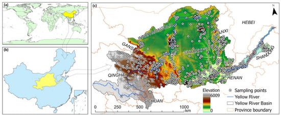
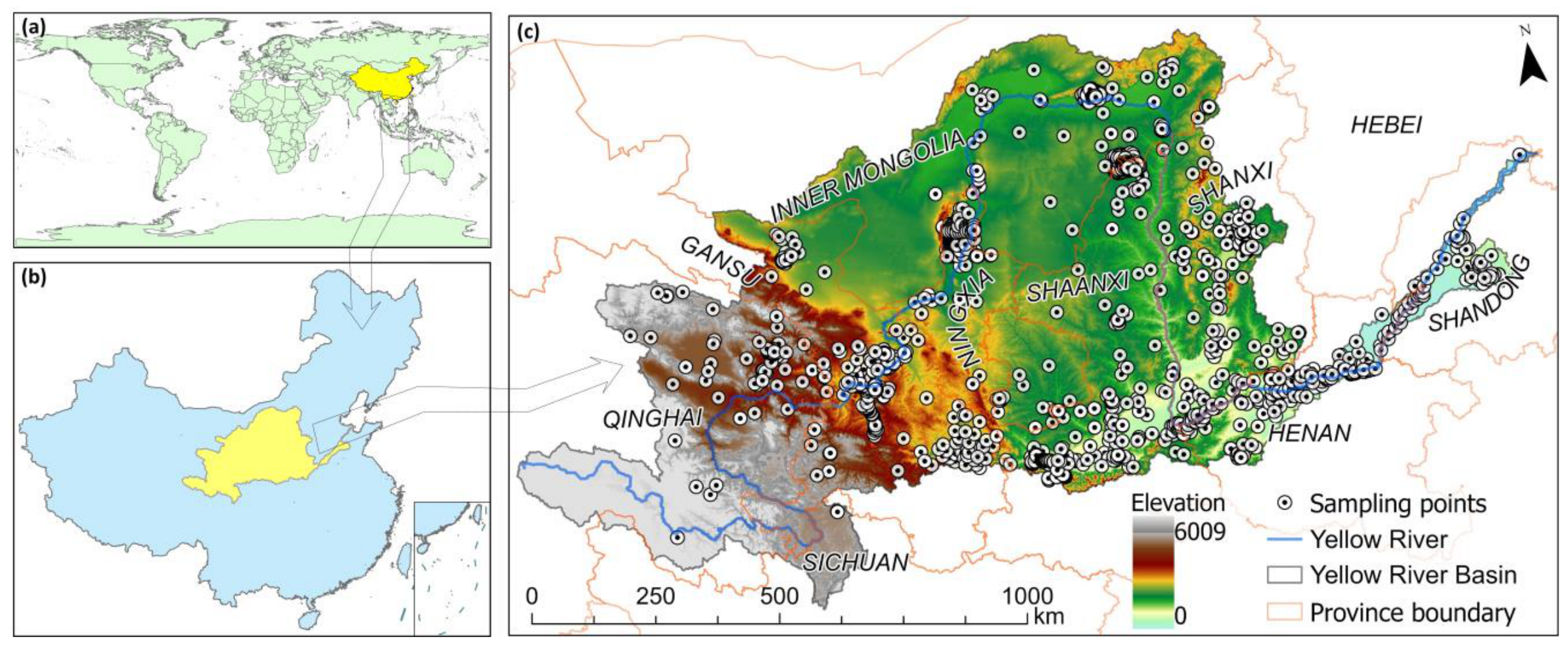
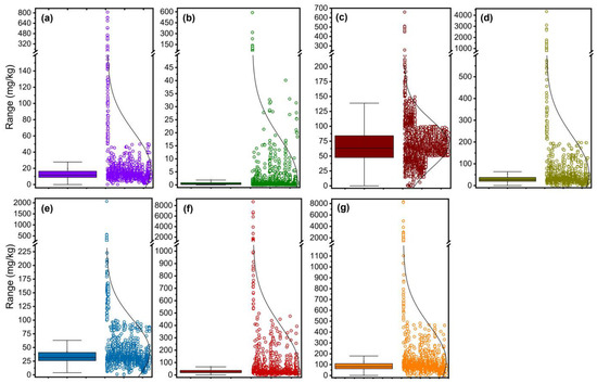
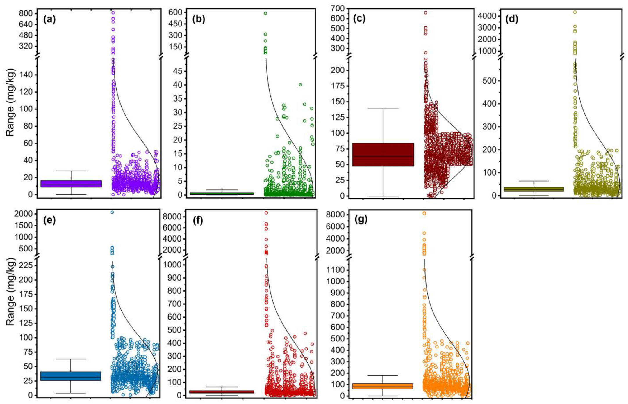
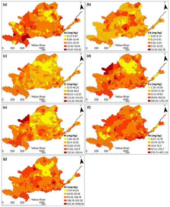
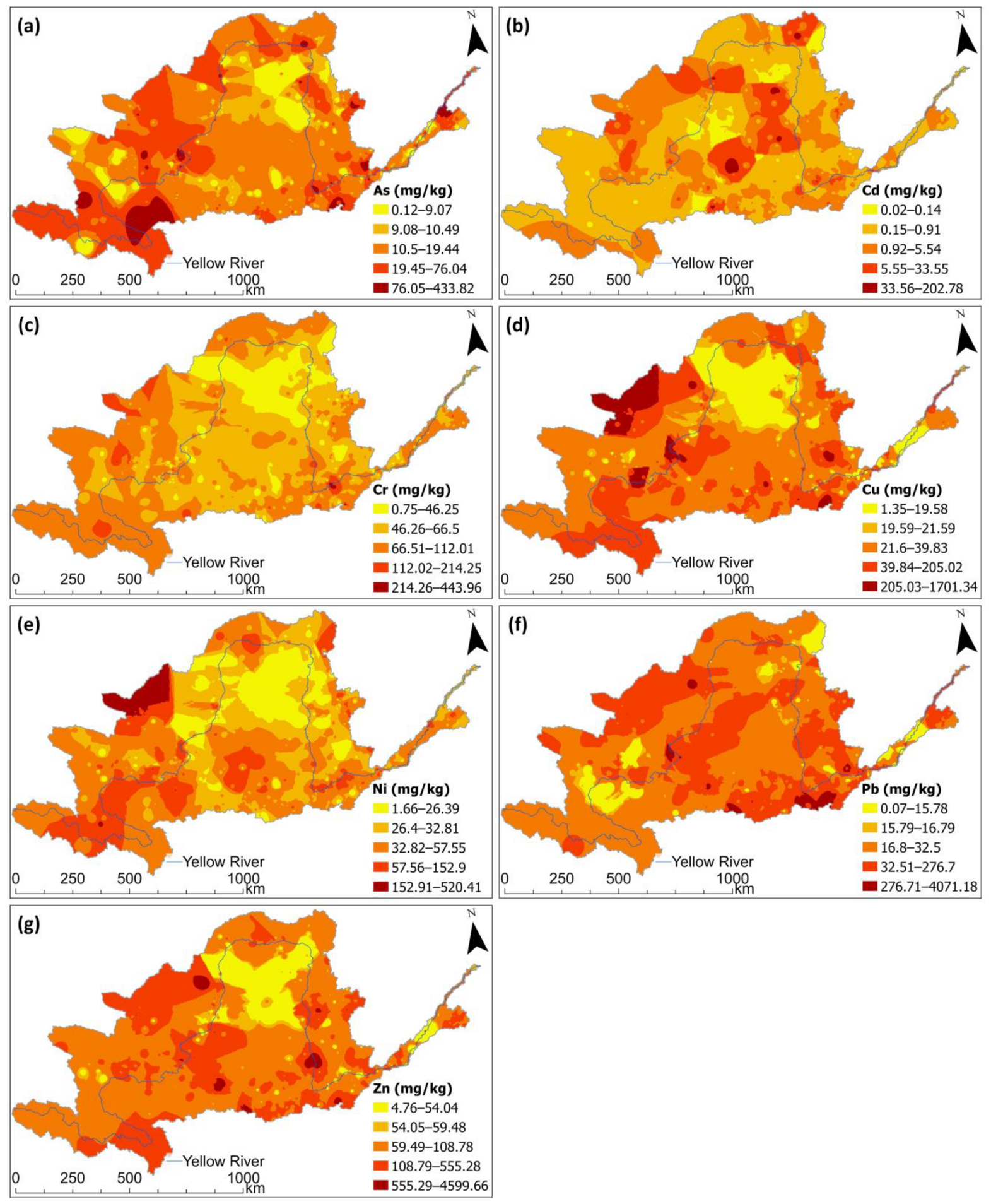
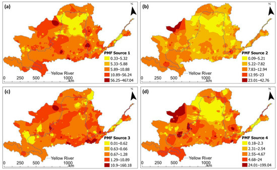
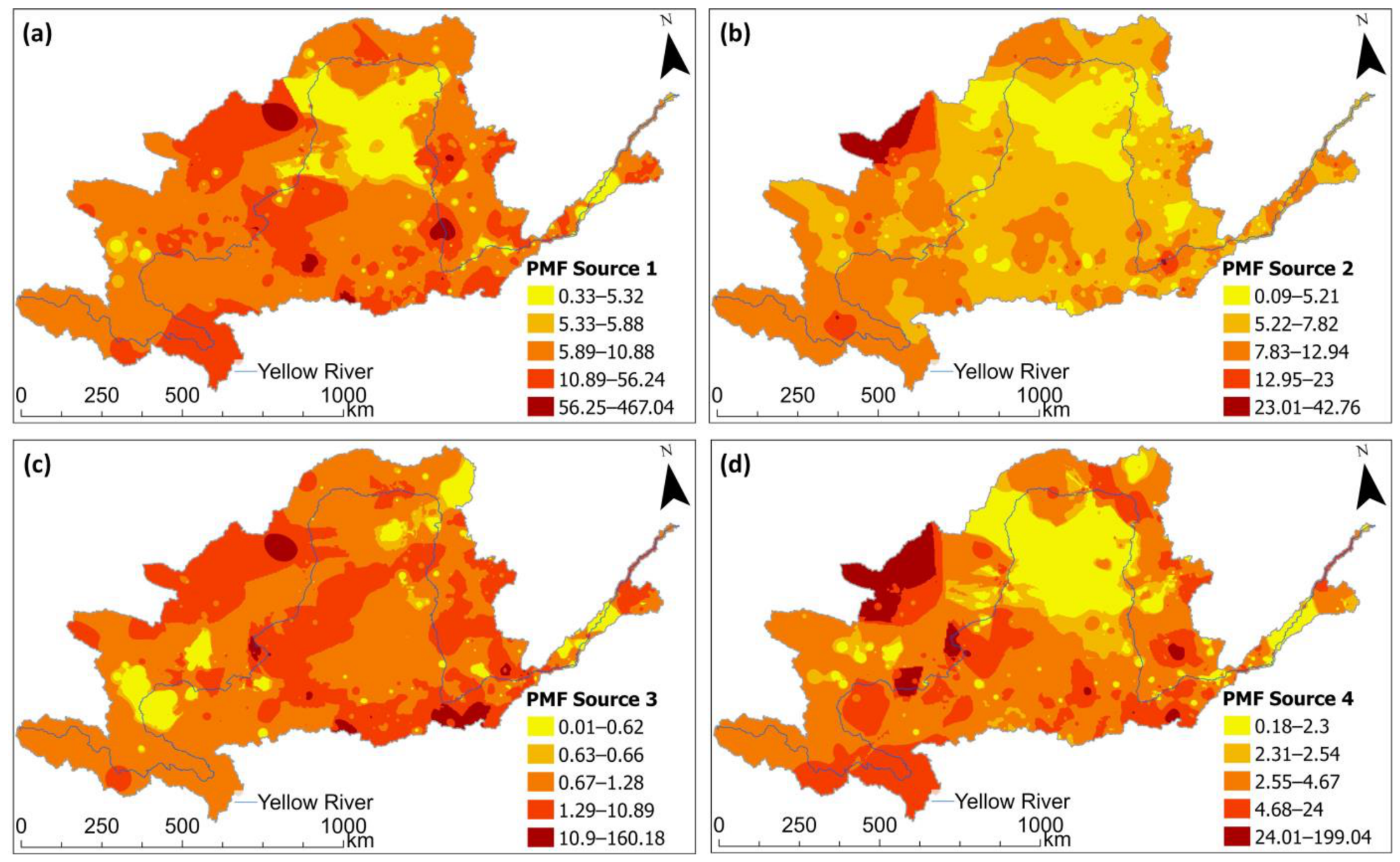
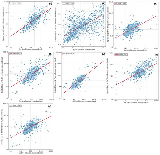
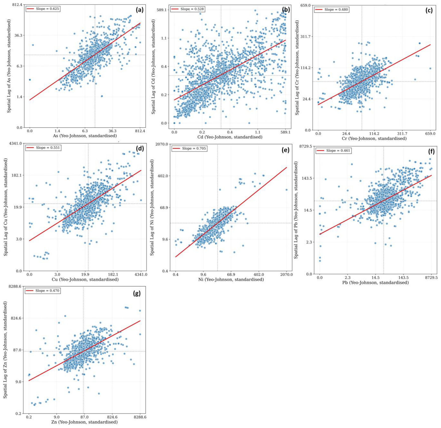
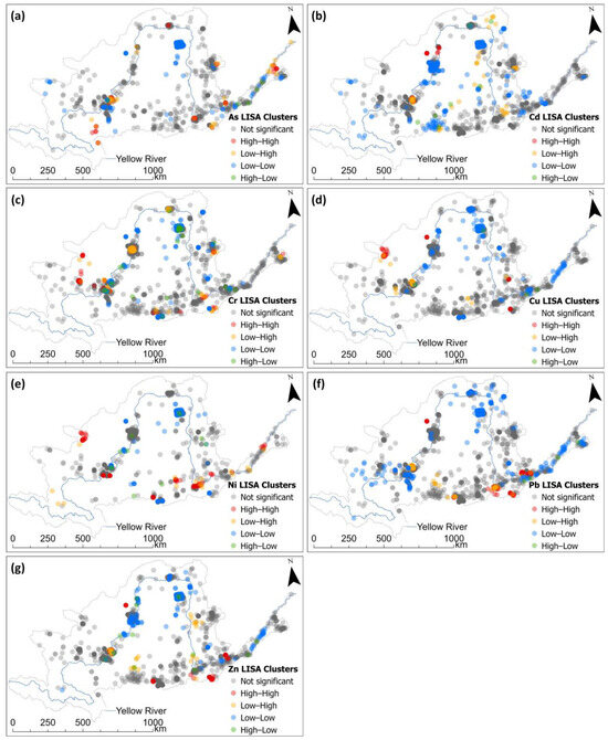
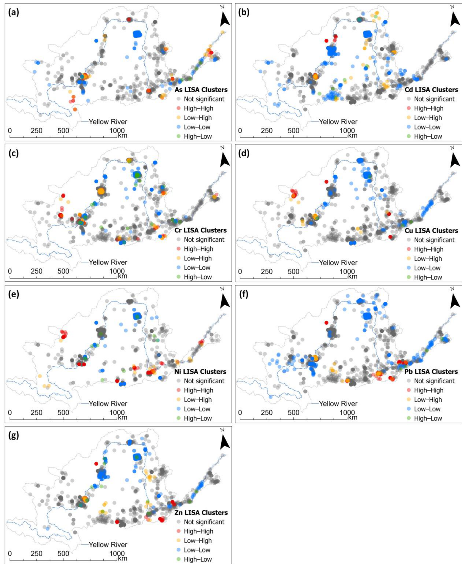
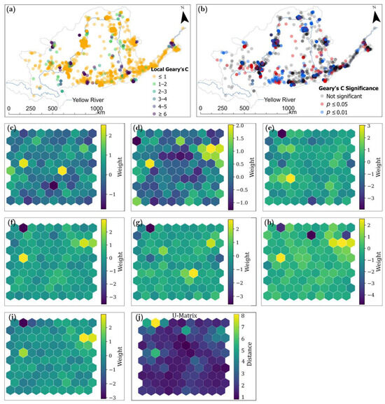
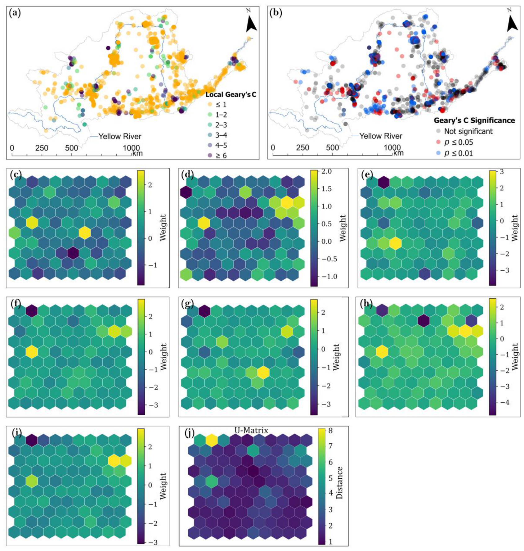
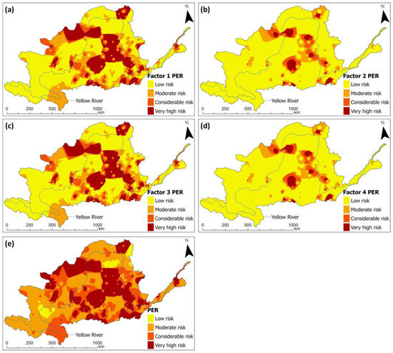
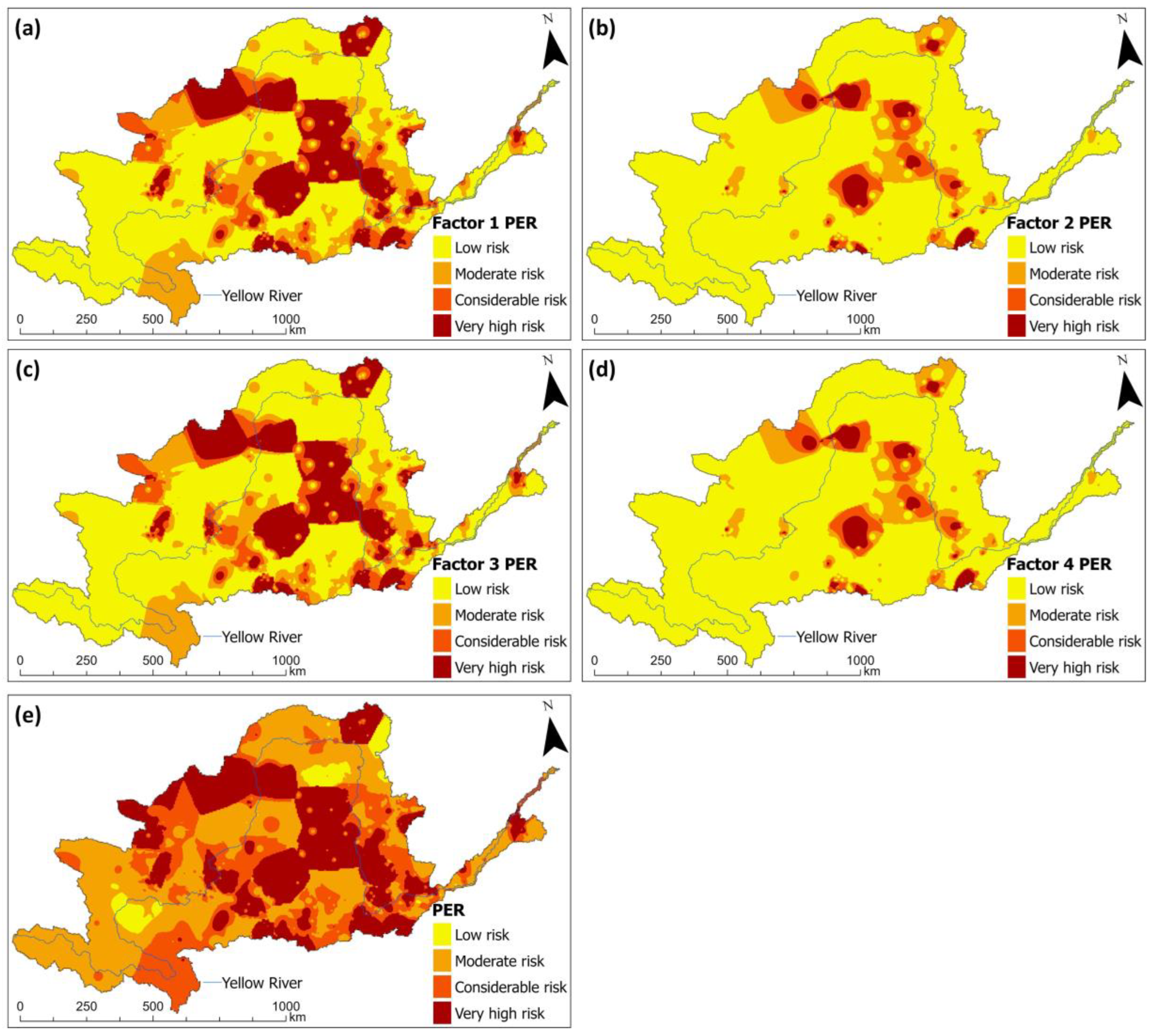
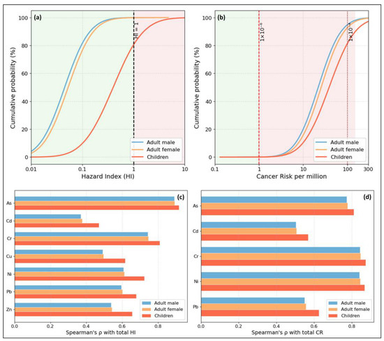
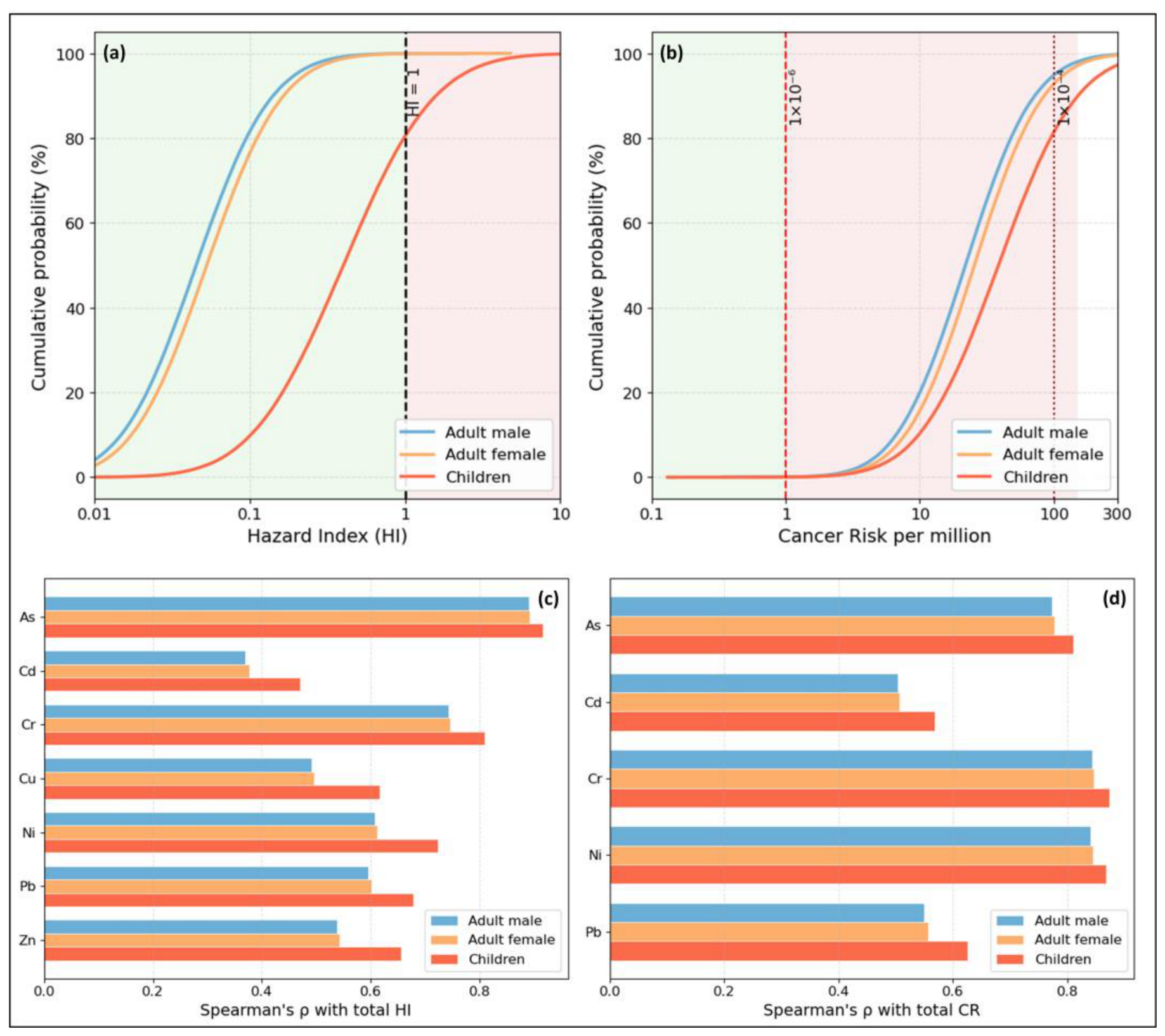
Disclaimer/Publisher’s Note: The statements, opinions and data contained in all publications are solely those of the individual author(s) and contributor(s) and not of MDPI and/or the editor(s). MDPI and/or the editor(s) disclaim responsibility for any injury to people or property resulting from any ideas, methods, instructions or products referred to in the content. |
© 2026 by the authors. Licensee MDPI, Basel, Switzerland. This article is an open access article distributed under the terms and conditions of the Creative Commons Attribution (CC BY) license.